Embed Size (px)
Citation preview

Broadband Spectrum Forecasting
ITU ASP COE TRAINING ON “WIRELESS BROADBAND ROADMAP DEVELOPMENT”
06-09 August 2016 Tehran, Islamic Republic of Iran

General Flow of Spectrum Requirement Calculation
• The ITU-R Report M.2290 provides methodology for estimation of future spectrum requirements of terrestrial IMT
• The spectrum requirements are calculated using the updated methodology in Recommendation ITU-R M.1768-1. (for the calculator and user guide refer to the Report ITU-R M.2290)

Radio Access Technology Group (RATG)
• RATG1 covers the digital cellular mobile systems, IMT-2000 systems and their enhancements
• The method in Recommendation ITU-R M.1768-1 estimates the spectrum demand for RATGs 1 and 2 only, but not those of RATG 3 (RLAN) and RATG 4
used by M.1768
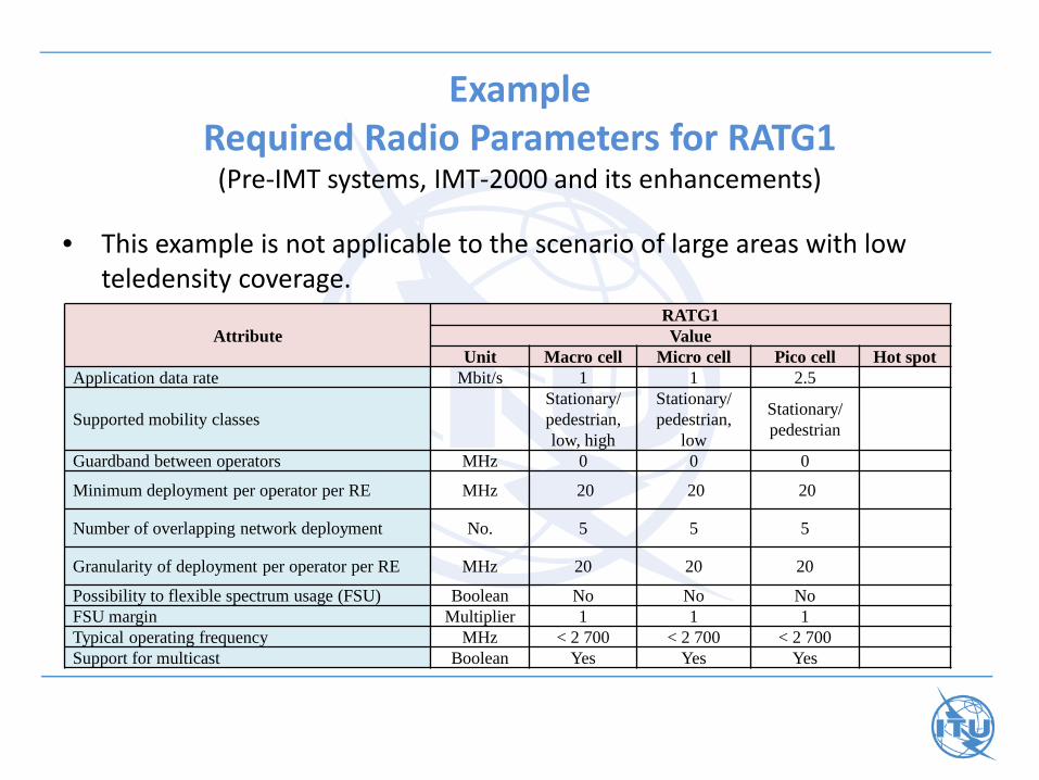
Example Required Radio Parameters for RATG1
(Pre-IMT systems, IMT-2000 and its enhancements)
• This example is not applicable to the scenario of large areas with low teledensity coverage.
Attribute RATG1 Value
Unit Macro cell Micro cell Pico cell Hot spot Application data rate Mbit/s 1 1 2.5
Supported mobility classes Stationary/ pedestrian, low, high
Stationary/ pedestrian,
low
Stationary/ pedestrian
Guardband between operators MHz 0 0 0
Minimum deployment per operator per RE MHz 20 20 20
Number of overlapping network deployment No. 5 5 5
Granularity of deployment per operator per RE MHz 20 20 20
Possibility to flexible spectrum usage (FSU) Boolean No No No FSU margin Multiplier 1 1 1 Typical operating frequency MHz < 2 700 < 2 700 < 2 700 Support for multicast Boolean Yes Yes Yes

Example Required Radio Parameters for RATG2
(IMT-Advanced systems as described in Recommendation ITU-R M.2012)
Attribute RATG2 Value
Unit Macro cell Micro cell Pico cell Hot spot Application data rate Mbit/s 50 100 1 000 1 000
Supported mobility classes Stationary/ pedestrian, low high
Stationary/ pedestrian,
low
Stationary/ pedestrian
Stationary/ pedestrian
Guardband between operators MHz 0 0 0 0 Minimum deployment per operator per RE MHz 50-100 50-100 100 100 Granularity of deployment per operator per RE MHz 20 20 20 20 Number of overlapping network deployment No. 1-4 1-4 1-4 1-4 Possibility to flexible spectrum usage (FSU) Boolean Yes Yes Yes Yes FSU margin Multiplier 1 1 1 1
Area spectral efficiency bit/s/Hz/ cell 2-4 2-5 3-6 5-10
Area spectral efficiency for multicasting bit/s/Hz/ cell 1-1.5 1-2.5 1.5-3 2.5-5
Typical operating frequency MHz < 6 000 < 6 000 < 6 000 < 6 000 Support for multicast Boolean Yes Yes Yes Yes

Example Required Radio Parameters for RATG3
(Existing radio LANs and their enhancements)
Attribute RATG3 Value
Unit Macro cell Micro cell Pico cell Hot spot Application data rate Mbit/s – – 50 100 Supported mobility classes – – Stationary/
pedestrian Stationary/ pedestrian
Support for multicast (yes = 1, no = 0) Yes

Example Required Radio Parameters for RATG4
(Digital mobile broadcasting systems and their enhancements)
Attribute RATG4 Unit Macro cell
Application data rate Mbit/s 2 Supported mobility classes All (Stationary/pedestrian, low and high) NOTE 1 – Only macro cell is considered for RATG4.

Spectral Efficiency
• In case of multicast, since the spectral efficiencies of the two transmission modes can be significantly different, separate area spectral efficiency values are needed.
Teledensity RATG No. rat
Radio environments Macro cell Micro cell Pico cell Hot-spot cell
Dense urban (bit/s/Hz/cell)
Suburban Rural
1,,1 ratη
1,,1 ratη

Definition of Some Terms Used in Report (SC)
• service categories (SC): a combination of service type and traffic class as shown in Table 1 Traffic class
Service type Conversa-
tional Stream-
ing Inter-active
Back-ground Peak bit rate
Super-high multimedia SC1 SC6 SC11 SC16 30 Mbit/s to 100 Mbit/s / 1Gbit/s
High multimedia SC2 SC7 SC12 SC17 < 30 Mbit/s
Medium multimedia SC3 SC8 SC13 SC18 < 2 Mbit/s Low rate data and low multimedia
SC4 SC9 SC14 SC19 < 144 kbit/s
Very low rate data(1) SC5 SC10 SC15 SC20 < 16 kbit/s (1) This includes speech and SMS.

Definition of Some Terms Used in Report (SC)
• Other parameters are needed in capacity calculations
Service category SC1 SC2 – SC20 Mean packet size (bit/packet) – – Second moment(1) of packet size (bit/packet) – –
Allowed mean packet delay (s) – – Allowed blocking rate (%) – – (1) The second moment of a random variable is a scalar value that is related to
the variance of the random variable.

Definition of Some Terms Used in Report (SC)
• Traffic classes (QoS classes for IMT-2000 from the user perspective): – conversational class of service (VoIP and videoconferencing); – interactive class of service (data from remote equipment e.g. a
server); – streaming class of service (scheme of real-time streams); – background class of service (end-user, typically is a computer)
• The main distinguishing factor between these classes is how delay-sensitive the application is
• Based on Recommendation ITU-R M.1079 the conversational and streaming class are served with circuit switching and the background and interactive class with packet switching.

Definition of Some Terms Used in Report (SC)
• Service category parameters: – User density (users/km2) – Session arrival rate per user (sessions/(s ⋅ user)) – Mean service bit rate (bit/s) – Mean session duration (s/session) – Mobility ratio (in-building, pedestrian, vehicular).
– Jm is traffic splitting fraction for service environment m
Mobility in market study Mobility in methodology mobility class Speed (km/h) mobility class Speed (km/h)
Stationary 0 Stationary/pedestrian 0 < V < 4 Low 0 < V < 4 High 4 < V < 100 Low (fraction Jm) 4 < V < 50
Super-high 100 < V < 250 High (fraction 1 − Jm) 50 < V
m Jm 1 1 2 1 3 1 4 1 5 0.5 6 0
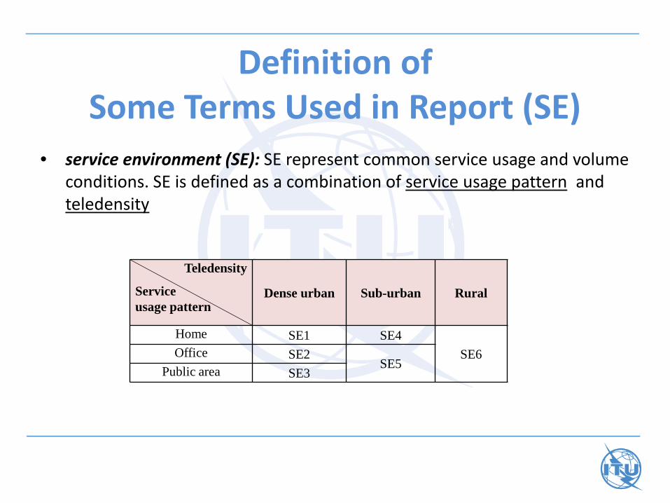
Definition of Some Terms Used in Report (SE)
• service environment (SE): SE represent common service usage and volume conditions. SE is defined as a combination of service usage pattern and teledensity
Teledensity
Service usage pattern
Dense urban Sub-urban Rural
Home SE1 SE4 SE6 Office SE2
SE5 Public area SE3

Definition of Some Terms Used in Report (SE)
• Possible user group and exemplary application of each SE User groups Applications
SE1 Private user, business user Voice, Internet access, games, e-commerce, remote education, multimedia applications
SE2 Business user, small and medium size enterprise
Voice, Internet access, video conferencing, e-commerce, mobile business applications
SE3 Private user, business user, public service user (e.g. bus driver, emergency service), tourist, sales people
Voice, Internet access, videoconferencing, mobile business applications, tourist information, e-commerce
SE4 Private user, business user Voice, Internet access, games, e-commerce, multimedia applications, remote education
SE5 Business user, enterprise Voice, Internet access, e-commerce, video conferencing, mobile business applications
SE6 Private user, farm, public service user Voice, information application
• Spectrum requirements shall first be calculated separately for each teledensity. • Final spectrum requirements is calculated by taking maximum value among
spectrum requirements for teledensity areas (dense urban, suburban and rural)

Definition of Some Terms Used in Report (RE)
• Radio environment (RE): REs are defined by the cell layers in a network consisting of hierarchical cell layers, i.e. macro, micro, pico and hot-spot cells.
• Naturally, a trade-off has to be found between network deployment costs and the spectrum requirement.
RE Teledensity Dense urban Sub-urban Rural
Macro cell 0.65 1.5 8.0 Micro cell(1) 0.1 0.1 0.1 Pico cell(1) 1.6E-3 1.6E-3 1.6E-3 Hot spot(1) 6.5E-5 6.5E-5 6.5E-5
* This example is not applicable to the scenario of large areas with low teledensity coverage. (1) It is assumed that the cell size of these environments is not teledensity dependent.
Example maximum cell area per RE(km2)*

Definition of Some Terms Used in Report (RE)
• In practice the total area of a particular service environment is only covered to a certain percentage X by each radio environment, e.g. by pico cells.
SE RE
Macro cell Microcell Pico cell Hot spot SE1 100 0 0 80 SE2 100 0 20 80 SE3 100 80 20 10 SE4 100 0 0 80 SE5 100 20 20 20 SE6 100 0 10 50
Example population coverage percentage of the radio deployment environments in each SE

Relationship Between SEs, RATGs and REs
• SEs and REs should be separately considered in the spectrum calculation such that traffic demands are forecasted over SE only, while total spectrum requirements are calculated with different RATGs and their possible RE.
• Spectrum requirements are calculated within each teledensity but final spectrum requirements need to be chosen as the maximum among spectrum requirements of all teledensities.
• Therefore, traffic in service environments should be accumulated with their corresponding teledensity first.

M.1768-02
A1 B1 A2 B2 A3 B3 A4 B4 A5 B5 A6 B6Traffic
Dense urbanHome SE1
B6B5B4B3B2B1A6A5A4A3A2A1
Dense urbanOffice SE2
Dense urbanPublic SE3
SuburbanHome SE4
SuburbanPublic SE5
RuralSE6
Service environments
RATG
Traffic
REs
Traffic
Aggregation oftraffic over SEs in
each teledensity
Spectrum
Spectrum requirementsfor a teledensity
Choose maximum Choose maximum
Spectrumrequirementsof RATG 1
Spectrumrequirementsof RATG 2
Mac
ro c
ell
Mic
ro c
ell
Pico
cell
Traffic distributionwithin a RATG
Traffic distributionamong RATGs
RATG 2RATG 1
two RATGs three radio environments

Steps of Calculation Algorithm
Step 1: Definition
Step2: Analyze Collected
Market Data
Step 3: Calculate
Traffic Demand
Step 4: Distribute
Traffic
Step 5: Calculate System
Capacity
Step 6: Calculate Unadjusted Spectrum
Requirement
Step 7: Apply
Adjustment
Step 8: Calculate Aggregate Spectrum
Requirement
Step 9: Final Spectrum
Requirement
RATGs, SEs, SCs, REs M.2072, M.2243
Area spectral efficiency • Mean delay • Blocking probability • Mean IP packet size • 2nd moment of IP packet size
Market attribute setting

Classification of Input Parameters

Analysis of the Collected Market Data (Collection of market data)
• The market data was collected by answering to the questionnaires. The questionnaires included the following items in order to survey future market and application trends:
• services and market survey for existing mobile services; – key market parameters; – service and market forecast for IMT, including:
• service issues; • market issues; • preliminary traffic forecast; • related information;
– service and market forecast for other radio systems; – driving forces of the future market; and – any other views on future services.
• The responses to the questionnaires are summarized and analyzed in Report ITU-R M.2072 (132 pages). More recent market data is provided in Report ITU-R M.2243.

Analysis of the Collected Market Data (Data Analysis)
M.1768-03
Step 1:List up
Applications/Services
Step 2:Specify traffic
attribute values of eachservice
Step 3:Specify market attributevalues of each service
Step 5:Calculate market
attribute values per eachSC and SE
Step 4:Map the services into
service category per eachSE
General process for the market data analysis

General Process for the Market Data Analysis List up Applications/Services – step 1
(Example application/service category and their traffic attributes)
Applications Services
Traffic attributes
Mean service bit rate
Average session
duration
Existing applications
Voice (multimedia and low rate data/ conversational) 64 kbit/s Video phone (medium multimedia/ conversational) 384 kbit/s
Packet
IM,e-mail (very low rate data/ background) 1 kbit/s Video mail (medium multimedia/ background) 512 kbit/s Mobile broadcasting (high multimedia/ streaming) 5 Mbit/s Internet access (high multimedia/) 10 Mbit/s
Town m
onitoring system
s
Voice (multimedia and low rate data/ conversational) 64 kbit/s Video communication (medium multimedia/conversational) 384 kbit/s Medium rate data transmission for town information monitoring (medium multimedia/interactive)
384 kbit/s
Low rate data transmission for Reservation of restaurants, etc. (very low rate data/interactive)
1 kbit/s
File transfer (super-high multimedia/ background) 50 Mbit/s
• The traffic attributes (step 2 of procedure) are extracted in above table last columns for: mean service bit rate and average session duration.

General Process for the Market Data Analysis Specify Market Attribute Values of Each Service-step 3
(Expected Response to Questionnaire on Market and Service) Applica
tions Services s: index
SC n
SE m
Market attributes
Use
r de
nsity
Um
,t,s
(use
rs/k
m2 )
Sess
ion
arri
val
rate
/use
r Q
m,t,
s (s
essi
ons/(
s ⋅ u
ser)
)
Mea
n se
rvic
e bi
t ra
te r s
(bit/
s)
Ave
rage
sess
ion
dura
tion
μ m,t,
s (s/
sess
ion)
Mobility ratio (%)
MRm,s
Stat
iona
ry
Low
Hig
h
Supe
r-hi
gh
Town monitoring systems
Town information monitoring s = 1
18 1
2 3
Reservation, s = 2
• In order to calculate the dynamic spectrum requirement of a RATG, the market attribute values need to be provided for individual time interval t.
• Each service can be mapped into the table composed of service type and traffic class as shown in above Table (step 4)

General Process for the Market Data Analysis Calculate Market Attribute Values per Each SC, SE and
Time Interval-step 5
• Market attribute values are provided separately for uplink and downlink.
Service category Service environment SE1 SE2 SE3 SE4 SE5 SE6
SC1 U1,t,1 Q1,t,1 μ1,t,1 r1,t,1
MR1,t,1
U2,t,1 Q2,t,1 μ2,t,1 r2,t,1
MR2,t,1
... ... ... U6,t,1 Q6,t,1 μ6,t,1 r6,t,1
MR6,t,1 SC2 U1,t,2
Q1,t,2 μ1,t,2 R1,t,2
MR1,t,2
... ... ... ... ...
SC3 ... ... ... ... ... ... ... ... ... ... ... ... ...

Parameters of Market Attribute Values
• User density (users/km2) of a certain service category:
Um,t,n and Um,t,s : the user density of service category n and the user density of service s inside service category n
• Session arrival rate per user (sessions/(s ⋅ user)): Qm,t,n and Qm,t,s : the session arrival rate per user of service category n and
the session arrival rate per user of service s inside service category n • Average session duration (s/session) :
where µm,t,n and µm,t,s denote the average session duration of service category n and the average session duration of service s inside service category n,
∑∈
=ns
stmntm UU ,,,,
ntm
nsstmstm
ntm U
QUQ
,,
,,,,
,,
∑∈=
∑∈
µ=µns
stmstmntm w ,,,,,,
ntmntm
stmstmstm QU
QUw
,,,,
,,,,,, =

Parameters of Market Attribute Values
• Mean service bit rate (bit/s) of a certain service category:
where:
where rm,t,n and rm,t,s denote the service data rate of service category n and the service data rate of service s inside service category n,
• Mobility ratio of a certain service category :
• where MR_marketm,t,n and MR_marketm,s denote the mobility ratio of
service category n and the mobility ratio of service s inside service category n
∑∈
=ns
stmstmntm rwr ,,,,,,ntmntmntm
stmstmstmstm
QUQU
w,,,,,,
,,,,,,,,
µµ
=
∑∈
=ns
smstmntm marketMRwmarketMR ,,,,, __

Parameters of Market Attribute Values
• The market study mobility ratios MR_market obtained above for stationary (sm), low (lm), high (hm) and super-high mobility (shm) need to be mapped into the methodology mobility ratios MR for stationary/pedestrian (sm), low (lm) and high mobility (hm). The mapping is done with Jm -factors.
• Mobility ratio for stationary mobility is obtained from: MR_smm,t,n = MR_market_smm,t,n + MR_market_lmm,t,n • Mobility ratio for low mobility is as follows: MR_lmm,t,n = Jm ⋅ MR_market_hmm,t,n • Mobility ratio for high mobility is as follows: MR_hmm,t,n = (1–Jm)⋅MR_market_hmm,t,n +MR_market_shmm,t,n

Distribution of Traffic Step 4 in Generic Calculation Algorithm
• The traffic obtained for each SE, time interval and SC will be distributed to possible RATGs and REs
• The following inputs are used for the traffic distribution: – The traffic values by SC and SE that are obtained as the outcome of Step 3
(Table 14) – SE definition matrix according to Step 1 including feasible REs and population
coverage percentages for each SE (Table 9) – RATG definition matrixes according to Step 1, – Distribution ratios ξm,t,n,rat,p (SC n in SE m and time interval t per cell or sector
of RATG rat and RE p) among available RATGs (Table 16)
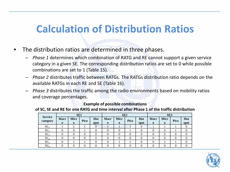
Calculation of Distribution Ratios
• The distribution ratios are determined in three phases. – Phase 1 determines which combination of RATG and RE cannot support a given service
category in a given SE. The corresponding distribution ratios are set to 0 while possible combinations are set to 1 (Table 15).
– Phase 2 distributes traffic between RATGs. The RATGs distribution ratio depends on the available RATGs in each RE and SE (Table 16).
– Phase 3 distributes the traffic among the radio environments based on mobility ratios and coverage percentages.
Service
category
SE1 SE2 SE3 Macr
o Micr
o Pico Hot spot
Macro
Micro Pico Hot
spot Macr
o Micr
o Pico Hot spot
SC1 1 1 1 0 1 1 1 0 1 1 1 0 SC2 0 0 1 0 0 0 1 0 0 0 1 0 SC3 0 0 0 0 0 0 0 0 0 0 0 0 SC4 0 0 0 0 0 0 0 0 0 0 0 0 SC5 0 1 1 0 0 1 1 0 0 1 1 0 SC6 0 0 0 0 0 0 0 0 0 0 0 0
Example of possible combinations of SC, SE and RE for one RATG and time interval after Phase 1 of the traffic distribution

Calculation of Distribution Ratios- phase 2
Available RATGs Distribution ratio (%)
RATG1 RATG2 RATG3 RATG4 1 100 – – – 2 – 100 – – 3 – – 100 4 – – – 100
1, 2 20 80 – 1, 3 20 – 80 1, 4 10 – – 90 2, 3 – 20 80 2, 4 – 10 – 90 3, 4 – – 10 90
1, 2, 3 20 20 60 1, 2, 4 10 10 – 80 1, 3, 4 10 – 10 80 2, 3, 4 – 10 10 80
1, 2, 3, 4 10 10 10 70
Example of distribution ratios among available RATGs, phase 2

Calculation of Distribution Ratios- phase 3
• Using the population coverage percentage information Xhs, Xpico, Xmicro and Xmacro of the hot-spot, pico, micro and macro radio environment, the algorithm distributes the following traffic ratios:
ξpico&hs = min(Xpico + Xhs, MR_sm) ξmicro = min(Xmicro, (MR_sm + MR_lm) − ξpico&hs) ξmacro = 1 − ξpico&hs − ξmicro • MR_sm and MR_lm are the ratios of offered traffic in the stationary and
low mobility classes, respectively. The equations assume that: MR_sm + MR_lm + MR_hm = 1 • Between hot-spot and pico cells the traffic is distributed according to the
relation of the population coverage ratios of hot-spot and pico cells: ξhs = ξpico&hs ⋅ Xhs/(Xpico + Xhs) ξpico = ξpico&hs ⋅ Xpico/(Xpico + Xhs)

Distribution of Session Arrival Rates
• The session arrival rate per area (sessions/(s ⋅ km2)) of service category n and service environment m distributed to RATG rat and radio environment p in time interval t, Pm,t,n,rat,p is calculated from the distribution ratio ξm,t,n,rat,p, user density Um,t,n and session arrival rate per user Qm,t,n by the following equation:
Pm,t,n,rat,p = ξm,t,n,rat,p ⋅ Um,t,n ⋅ Qm,t,n
• The traffic from all users in a cell needs to be accumulated. The session arrival rate/cell (sessions/(s ⋅ cell)) is calculated as:
• where Ad,p is the cell area (km2) of RATG rat in teledensity d and radio environment p, where d is uniquely determined by m
pdpratntmpratntm APP ,,,,,,,,, ⋅=′

Calculation of offered traffic
• Circuit switched traffic: – The offered traffic (Erlang/cell) by use of the session arrival rate
from the distribution functionality and the mean session duration µm,t,n :
– The aggregate values of the mean service bit rate rd,t,n,rat,p (bit/s) for teledensity d are obtained as follows:
• Packet-switched traffic:
– The offered traffic for service category n for RATG rat in radio environment p for teledensity d and different time interval t:
.
pratntmP ,,,,′
∑∈
µ′=ρdm
ntmpratntmpratntd P ,,,,,,,,,,
pratntd
dmntmntmpratntm
pratntd
rPr
,,,,
,,,,,,,,
,,,, ρ
µ′
=∑∈
∑∈
µ′=dm
ntmntmpratntmpratntd rPT ,,,,,,,,,,,,

Determination of the Required System Capacity step 5 of Generic Calculation Method
(circuit switched traffic)
• The required system capacity (i.e. reservation based) service categories is determined by the number of service channels needed to achieve a specified blocking probability, and the channel data rate. Inputs are: – Offered traffic in Erlangs per cell or sector ρd,t,n,rat,p – Service channel data rate rd,t,n,rat,p for service category n – Maximum allowable blocking probability πn,
• multi-dimensional Erlang –B formula implemented

Determination of the Required System Capacity step 5 of Generic Calculation Method
(Packet-Switched Traffic)
• The system capacity needed to fulfil each service category’s mean delay requirement is determined using a queuing model applicable for independent arrival times of packets and arbitrary distribution of packet size.
• In queuing theory the model is known as an M/G/1 queuing model with non-pre-emptive priorities or head-of-the-line queuing system [Klienrock, 1976]. Input parameters are:
– For each SC the offered base traffic per SE per cell Td,t,n,rat,p (bit/(s ⋅ cell)) – Mean sn (bits/packet) and second moment sn
(2) (bits2/packet) of the IP packet size distribution of each SC n
– The required mean delay Dn of each service category (given in Table 5) – The priority ranking of all SCs n with n = 1, 2,..., Nps. It is assumed that the SC n = 1 has
the highest priority, i.e. IP packets of SC n = 1 are served first. The SC n = Nps has the lowest priority. The priority ordering of the SCs is equivalent to the SC numbering.

Determination of the Spectrum Requirements step 6 of Generic Calculation Method
(steps 1 and 2) • Step 1: The capacity calculation so far has been separately for uplink
and downlink. The capacity requirements for uplink and downlink are combined, separately for packet and circuit switched capacity requirements:
Cd,t,rat,p,cs (bit/(s ⋅ cell)) = Cd,t,rat,p,cs,UL + Cd,t,rat,p,cs,DL
Cd,t,rat,p,pcs (bit/(s ⋅ cell)) = Cd,t,rat,p,ps,UL + Cd,t,rat,p,ps,DL
• Step 2: The capacity requirements of circuit switched and packet switched traffic are combined, i.e.:
Cd,t,rat,p = Cd,t,rat,p,cs + Cd,t,rat,p,ps • In the case of mobile multicast capacity requirements, this is calculated
similarly as the sum of packet and circuit switched multicast capacity requirements.

Determination of the Spectrum Requirements step 6 of Generic Calculation Method
(step 3) • Step 3: The spectrum requirement for RATG rat in teledensity d, time
interval t and radio environment p are calculated by applying the area spectral efficiency factors. The spectrum requirement is obtained from:
where ηd,rat,p (bit/(s ⋅ Hz ⋅ cell)) is the area spectral efficiency in teledensity
d, RATG rat and radio environment p. • In the case of mobile multicast capacity requirements, the corresponding
spectrum requirement Fd,rat,p,mm is calculated separately, using the appropriate spectral efficiency ηd,rat,p value. This spectrum requirement is then added to the spectrum requirement of user individual communication:
Fd,t,rat,p = Fd,t,rat,p + Fd,t,rat,p,mm
pratd
prattdprattd
CF
,,
,,,,,, η=

Applying necessary adjustments step 7 of Generic Calculation Method
(step 1) • Spectrum requirements are aggregated over radio environments.
Adjustments are made taking into account the minimum spectrum requirement for a network deployment, necessary guardbands and the impact of the number of operators.
• Step1: We assume the spectrum distribution among operators within one RATG is fixed. Furthermore we assume each operator has available the same share of the total spectrum. Then the unadjusted spectrum per operator is:
Fd,t,rat,p = Fd,t,rat,p/No where No is the number of operators

Applying necessary adjustments step 7 of Generic Calculation Method
(step 2)
• Step 2: Spectrum can in general only be used with granularity GrnSpecrat,p and the minimum bandwidth MinSpecrat,p required for being able to allocate a single carrier to each cell in a wide area network, taking into account the frequency reuse factor. The spectrum requirement needs to be adjusted accordingly:
Fd,t,rat,p = 0 if Fd,t,rat,p =0 Fd,t,rat,p = MinSpecrat,p if 0 < Fd,t,rat,p ≤ MinSpecrat,p Fd,t,rat,p = MinSpecrat,p+GrnSpecrat,p ⋅(Fd,t,rat,p-MinSpecrat,p) /GrnSpecrat,p if
MinSpecrat,p < Fd,t,rat,p
• where means rounding to the next largest integer and MinSpecrat,p and GrnSpecrat,p are obtained from Tables 10a and 10b.

Applying necessary adjustments step 7 of Generic Calculation Method
(step 3) • Step 3: For RATG1, it is assumed that pico cell and hot-spot radio environments
are not spatially coexisting. Therefore, the maximum of both REs needs to be taken. The macro and micro cell REs are assumed to spatially coexist with the pico cell and hot-spot RE, respectively. Therefore, for RATG1, the spectrum requirements of macro and micro environment need to be added to the maximum of the pico and hot-spot radio environment:
Fd,t,rat = Fd,rat,macro + Fd,t,rat,micro + max(Fd,t,rat,pico, Fd,t,rat,hotspot) • For RATG2, the recent development of heterogeneous networks is leading to the
direction that the different cell types are capable of being deployed on the same spectrum more efficiently than previously anticipated. Therefore, for RATG2, the spectrum requirements of maximum of macro and micro environment need to be added to the maximum of the pico and hot-spot radio environment:
Fd,t,rat = max (Fd,t,rat,macro, Fd,t,rat,micro) + max (Fd,t,rat,pico, Fd,t,rat,hotspot) • Then, the total required spectrum for all operators is: Fd,t,rat = Fd,t,rat ⋅ No

Applying necessary adjustments step 7 of Generic Calculation Method
(step 4) • Step 4: Guardbands are considered. It is assumed that the spectral
efficiency figures already take into account a guardband that is required between carriers of the same operator. This means that the spectral efficiency figures also are based on the assumption that either an adjacent carrier has no influence, or the influence is already included in the spectral efficiency figure. The guardband between operators introduces additional spectrum requirements:
Fd,t,rat = Fd,t,rat + (No – 1) ⋅ Grat where the values of guardband between operators Grat are input
values given by Tables 10a and 10b.

Calculate aggregate spectrum requirements step 8 of Generic Calculation Method
(step 1) • Step 1: The time dependency of the spectrum requirement is considered.
The two options below, i.e. a) and b), are to calculate the spectrum requirements without or with FSU possibility.
• Step 2: Teledensity environments are spatially non-overlapping areas, thus the teledensity environment having the highest spectrum demand determines the spectrum requirement for a RATG.
• Step 3: Where a common estimation is required for a group of countries, maximum of market study individual spectrum requirements should be taken.
• Step 4: Optionally, as a final step, the total required spectrum is the Step 8. a) Without FSU possibility all the RATG demands are summed: b) With FSU possibility the spectrum for FSU enabled RATGs and
non-FSU enabled RATGs are added together:
∑=rat
ratFF
nonFSUratRATsFSUrat
FSU FFF ,}{
∑∉
+=

Thank You