Heriot-Watt University Research Gateway

Heriot-Watt University

Brittle failure and fracture reactivation in sandstone by fluid injectionCharalampidou, Elli-Maria Christodoulos; Stanchits, Sergei; Kwiatek, Grzegorz; Dresen,GeorgPublished in:European Journal of Environmental and Civil Engineering

DOI:10.1080/19648189.2014.896752

Publication date:2015

Document VersionPeer reviewed version

Link to publication in Heriot-Watt University Research Portal

Citation for published version (APA):Charalampidou, E-M. C., Stanchits, S., Kwiatek, G., & Dresen, G. (2015). Brittle failure and fracture reactivationin sandstone by fluid injection. European Journal of Environmental and Civil Engineering, 19(5), 564-579. DOI:10.1080/19648189.2014.896752

General rightsCopyright and moral rights for the publications made accessible in the public portal are retained by the authors and/or other copyright ownersand it is a condition of accessing publications that users recognise and abide by the legal requirements associated with these rights.

If you believe that this document breaches copyright please contact us providing details, and we will remove access to the work immediatelyand investigate your claim.

Brittle failure and fracture reactivation in sandstone by fluid injection.

Charalampidou Elli-Maria a, Stanchits Sergei b, Kwiatek Grzegorz a,

Dresen Georg a

a GFZ German Research Centre for Geosciences, Telegrafenberg D423, 14473 Potsdam, Germany b TerraTek A Schlumberger Company, 1935 Fremont Drive, 84104 Salt Lake City, USA

Corresponding author: Charalampidou Elli-Maria, Telephone number: +49 331 288

28834, Fax number: +49 331 288 1328, Email address: elmachar@gfz-potsdam.de

Brittle failure and fracture reactivation in sandstone by fluid injection.

We performed laboratory experiments on sandstone specimens to study brittle

failure and the reactivation of an experimentally produced failure plane induced

by pore-pressure perturbations using constant force control in high compressive

stress states. Here we focus on the shear failure of a dry sample and the later on

induced fracture plane reactivation due to water injection. Acoustic Emission

(AE) monitoring has been used during both experiments. We also used ultrasonic

wave velocities to monitor pore fluid migration through the initially dry

specimen. To characterise AE source mechanisms, we analysed first motion

polarities and performed full moment tensor inversion at all stages of the

experiments. For the case of water injection on the dry specimen that previously

failed in shear, AE activity during formation of new fractures is dominated by

tensile and shear sources as opposed to the fracture plane reactivation, when

compressive and shear sources are most frequent. Furthermore, during the

reactivation of the latter, compressive sources involve higher compressive

components compared to the shear failure case. The polarity method and the

moment tensor inversion reveal similar source mechanisms but the latter provides

more information on the source components.

Keywords: water injection; reactivation of pre-existing fractures; polarity

method; moment tensor inversion

1. Introduction

A significant issue associated with geothermal energy extraction is the necessity to

inject fluids (e.g. water) into wells in order to enhance the permeability of the reservoir

and the productivity of the geothermal well. Such activity tends to induce microseismic

events (e.g., Zoback and Harjes, 1997; Majer & Paterson, 2007; Majer et al., 2007;

Cuenot et al., 2008), although there is not a strict one to one correlation in time and

space between fluid injection and induced seismicity (Majer & Paterson, 2007). An

extensive survey on induced seismicity from fluid injection into igneous and

sedimentary geothermal reservoirs in Europe can be found in (Evans et al., 2012).

Induced seismicity may be caused by different processes (Majer et al., 2007).

For example, pore pressure increase and volume changes due to fluid injection are

considered to be the main causes of induced seismicity in geothermal environments.

However temperature changes and chemical alteration of fracture surfaces may also

result in seismic events. Given that geothermal systems are commonly located within

faulted regions subjected to elevated stresses (Evans et al., 2012), an increase in pore

pressure due to injection may result in activation of pre-existing faults or sets of

fractures present in the reservoirs. Non-sealed fractures and faults may act as

preferential flow paths and enhance the productivity of a geothermal reservoir (Tezuka

and Niitsuma, 2000). However, the reactivation of faults may produce earthquakes

generating substantial concern in local communities (e.g., Giardini, 2009, Holland,

2013).

Here we investigate the mechanisms governing the formation and subsequent

reactivation of a set of fractures (or failure planes) due to fluid injection at controlled

laboratory conditions. We first describe the sample material and the experimental

procedures. Results of the mechanical tests are discussed in terms of advanced acoustic

methods, which capture the spatio-temporal evolution of fracturing and fracture

reactivation as a function of stress conditions and pore-pressure history.

2. Sample material and experimental methods

2.1 Material and experimental procedure

Flechtingen sandstone (Flechtingen quarry, NE Germany), a Lower Permian rock

(Ellenberg et al., 1976) consisting of 65-75% quartz and 15% calcite and illite (Zang et

al., 1996), was used in this study. The mean quartz grain size ranges from 0.1 to 0.5

mm, the initial porosity varies between 5.5% and 9%, and the permeability is between

10-16 to 10-17 m2 (Stanchits et al., 2011). The uniaxial compression strength of this

material in dry samples ranges from 63 to 107 MPa and from 50 to 79 MPa in wet

samples (Zang et al., 1996). Cylindrical specimens of 50 mm diameter and 120 mm

length were cored parallel to bedding plane.

Experiments were performed using a servo-hydraulic loading frame from

Material Testing Systems (MTS) with a load capacity of 4600 kN and a triaxial cell

sustaining a confining pressure up to 200 MPa. Two Quizix pore-pressure pumps

controlled the applied pore pressure and measured the injected fluid volume. Samples

were jacketed in a neoprene membrane. To allow water migration and in-situ saturation

of the specimen, no lubrication was applied to its top and base. AE activity and

ultrasonic P-wave velocities were recorded during each experiment (in-situ monitoring).

We present results from one cylindrical Flechtingen sandstone specimen, which

was subjected to different loading stages. First, isostatic pressure was applied to the dry

intact specimen. At 40 MPa confining pressure, the same specimen was loaded under

triaxial compression until shear failure occurred. Confining pressure was then increased

to 80 MPa to lock the shear failure plane. Afterwards, the sample was loaded again

under triaxial compression close to peak stress. Subsequently, a switching of loading

regimes was set: first constant stress regime until a certain displacement limit followed

by constant displacement rate regime. The reactivation of the pre-existing fracture plane

was investigated under a constant stress regime, while in previous works (see also

Stanchits et al., 2011, Mayr et al., 2011) a constant displacement regime was used

instead. In order to make a safe sliding it was necessary in our experimental procedure

to introduce a threshold level of maximum allowed sliding and to make an automatic

switch to constant displacement regime. While the differential stress was kept constant,

distilled water was injected at the specimen base at a constant pore pressure of 5 MPa,

until sliding along the pre-existing failure plane started. During the subsequent

displacement regime, the specimen was loaded for a while and then it was allowed to

creep until it became fully saturated.

2.2. Experimental methods

Sixteen P-wave sensors were glued directly to the surface of the specimen and sealed in

a neoprene jacket with two-component epoxy. The geometry of the sensor network (see

Fig. 1) provided a good azimuthal coverage of the AE events. These P-wave ultrasonic

sensors, which consisted of PZT piezoceramic disks of 5 mm diameter and 2 mm

thickness placed on brace housings, had a resonant frequency of 1 MHz. Furthermore,

two similar P-wave sensors were embedded in two metallic spacers placed at the bottom

and top end of the specimen (transmitting and receiving only along the vertical direction

– sensor pair 16-15 is not shown in Fig.1). AE signals were amplified by 40 dB, using

Physical Acoustic Corporation (PAC) preamplifiers (see also Stanchits et al., 2009).

Half of the sensors that were used for ultrasonic transmission (marked with light bold

numbers in Fig. 1b) were emitting every 30 seconds by application of rectangular

electrical pulse of 100 V amplitude and 3µs duration. During ultrasonic transmission,

these sensors were disconnected from the preamplifiers. The remaining sensors (shown

in dark bold numbers in Fig. 1b) were recording the pulses. P-wave velocity

measurements were made along 65 different transmitter-receiver traces (1 vertical trace

and 64 horizontal and inclined traces from pulses of 8 transmitters recorded at 8

receivers placed around the specimen). Full AE waveforms and ultrasonic signals were

stored continuously in a 16 channel transient recording system (DAXBox, PRÖKEL,

Germany) with an amplitude resolution of 16 bit at 10 MHz sampling rate (Stanchits et

al., 2006, 2009). During the experiments, all ultrasonic signals and AE waveforms were

recorded in eight internal hard disks of the recording system with no dead time between

the sequential signals.

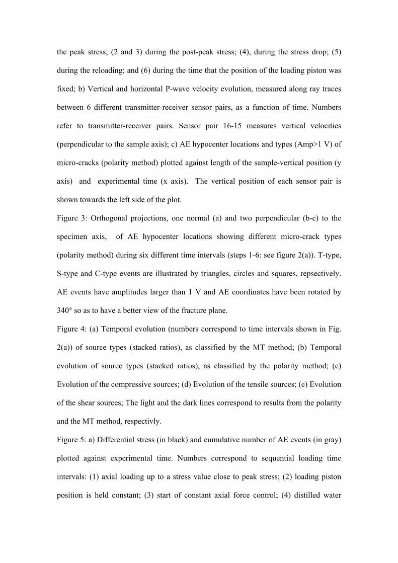
Figure 1: a) Schematic view of the specimen geometry, showing the positions of the P-wave sensors; b) Map of the azimuthial coverage of P-wave sensors used as receivers and transmitters (in light bold colours) and as receivers (in dark bold colours) during the experiment.

After each experimental stage both ultrasonic signals and AE waveforms were

automatically discriminated. The P-wave onset-times were calculated by applying an

automatic picking based on the Akaike information criterion (Leonard and Kennett,

1999). The AE hypocentre locations were calculated by minimising travel time

residuals using the downhill simplex algorithm (Nelder and Mead, 1965), considering

time-dependent variations in P-wave velocities and employing an anisotropic

heterogeneous ultrasonic velocity model, consisting of five horizontal layers (Stanchits

et al., 2006). Time dependent anisotropic velocities inside each layer were periodically

updated using ultrasonic transmission measurements.

AE source mechanisms were used to characterise the distribution of different

crack types associated with sample failure and fracture activation. First motion

amplitudes were picked automatically and first motion polarities were used to

distinguish the AE source types (equivalent to tensile, shear and compressive sources).

An average first motion polarity (pol) for each AE event was calculated as the mean of

all sensor recordings (excluding sensors 17-18 and 16-15, which were used only for

velocity measurements). AE events were defined as T-, S- and C-type sources,

characterised by -1≤ pol< -0.25 (tensile), -0.25≤ pol≤ +0.25 (shear) and +0.25 < pol≤ +1

(compressive), respectively (Zang et al., 1998). The AE source types, corresponding to

events with waveforms recorded by fourteen sensors surrounding the specimen (sensors

17-18 were excluded since they did not record AEs), were plotted together with their

hypocentre locations.

Additionally, the Moment Tensors (MT) of AE events were calculated. The

effects of incident angle, sensor coupling and damage evolution were taken into account

for the MT solutions (see Kwiatek et al., 2013). To examine the nature of the AE

sources, the MTs were decomposed into isotropic (ISO), compensated linear vector

dipole (CLVD) and double-couple (DC) components, following (Vavrycuk, 2001). The

classification of AE sources was based on the contribution of the DC component to each

source, similar to other laboratory (Ohtsu, 1995; Graham et al., 2010) and field studies

(Ohtsu, 1995; Kirkpatrick et al., 1996). In this paper, AE events with DC components

exceeding 70% were grouped as shear sources, events with DC components between

30% and 70% were classified as mixed-mode sources (having significant isotropic and

shear components), and events with DC components less than 30% were considered

tensile or compressive sources (depending on the sign of the ISO and CLVD

components, with compressive sources characterised by a negative sign). A sub-

classification of tensile and compressive sources, characterised by a higher or lower

volume change, was performed based on their ISO component (i.e., higher or lower than

30%, respectively).

3. Results

3.1. Fracturing of dry intact specimen

An intact cylindrical Flechtingen sandstone specimen was loaded in triaxial

compression at 40 MPa confining pressure. AE feedback control of the loading rate was

performed during axial loading (Lockner et al., 1991; Stanchits et al., 2006; Stanchits et

al., 2011). In the early stages of deviatoric loading the specimen was subjected to

constant displacement rate of 20 µm/min (corresponding to a nominal axial strain rate

of 2.77x10-6 s-1). With increasing AE activity above a defined threshold level, the

displacement rate was decreased, or the piston was retracted as required to unload the

specimen until the AE activity decreased below the defined threshold level (Lockner et

al., 1991, 1992, Stanchits et al., 2011).

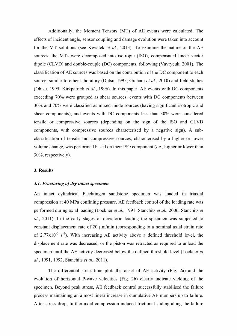
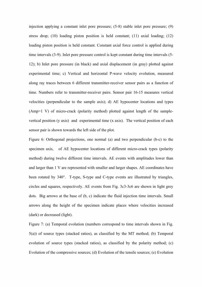
The differential stress-time plot, the onset of AE activity (Fig. 2a) and the

evolution of horizontal P-wave velocities (Fig. 2b) clearly indicate yielding of the

specimen. Beyond peak stress, AE feedback control successfully stabilised the failure

process maintaining an almost linear increase in cumulative AE numbers up to failure.

After stress drop, further axial compression induced frictional sliding along the failure

plane again at a constant AE rate. P-wave velocities parallel and perpendicular to the

sample axis indicate evolution of significant velocity anisotropy due to closure of

horizontal cracks and the formation of axial micro-cracks (Fig. 2b) (Stanchits et al.,

2011).

Figure 2: a) Differential stress and cumulative number of AE events plotted against experimental time. Numbers correspond to sequential loading time intervals: (1) up to the peak stress; (2 and 3) during the post-peak stress; (4), during the stress drop; (5) during the reloading; and (6) during the time that the position of the loading piston was fixed; b) Vertical and horizontal P-wave velocity evolution, measured along ray traces between 6 different transmitter-receiver sensor pairs, as a function of time. Numbers refer to transmitter-receiver pairs. Sensor pair 16-15 measures vertical velocities (perpendicular to the sample axis); c) AE hypocenter locations and types (Amp>1 V) of micro-cracks (polarity method) plotted against length of the sample-vertical position (y axis) and experimental time (x axis). The vertical position of each sensor pair is shown towards the left side of the plot.

The AE hypocentre distribution shows a maximum of events clustering in the

centre part of the sample (Fig. 2c). The location error is smaller than 2 mm (residuals

smaller than 0.5 µs). T-, S- and C-type sources, corresponding to AE events with

preamplified amplitudes larger than 1 V, are illustrated by triangles, circles and squares,

respectively. The AE cluster in the specimen centre evolving with time is in good

agreement with a strong degradation of horizontal P-wave velocities along the central

traces between sensors 4-2, 8-6 and 9-10 (Fig. 1, Fig. 2b).

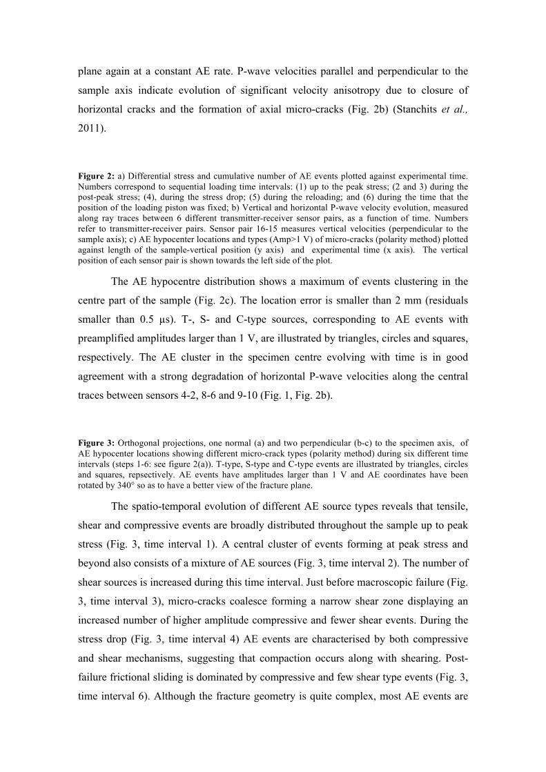
Figure 3: Orthogonal projections, one normal (a) and two perpendicular (b-c) to the specimen axis, of AE hypocenter locations showing different micro-crack types (polarity method) during six different time intervals (steps 1-6: see figure 2(a)). T-type, S-type and C-type events are illustrated by triangles, circles and squares, repsectively. AE events have amplitudes larger than 1 V and AE coordinates have been rotated by 340° so as to have a better view of the fracture plane.

The spatio-temporal evolution of different AE source types reveals that tensile,

shear and compressive events are broadly distributed throughout the sample up to peak

stress (Fig. 3, time interval 1). A central cluster of events forming at peak stress and

beyond also consists of a mixture of AE sources (Fig. 3, time interval 2). The number of

shear sources is increased during this time interval. Just before macroscopic failure (Fig.

3, time interval 3), micro-cracks coalesce forming a narrow shear zone displaying an

increased number of higher amplitude compressive and fewer shear events. During the

stress drop (Fig. 3, time interval 4) AE events are characterised by both compressive

and shear mechanisms, suggesting that compaction occurs along with shearing. Post-

failure frictional sliding is dominated by compressive and few shear type events (Fig. 3,

time interval 6). Although the fracture geometry is quite complex, most AE events are

located within a distinct failure plane, inclined at about 25°-27° to the axis of the

specimen.

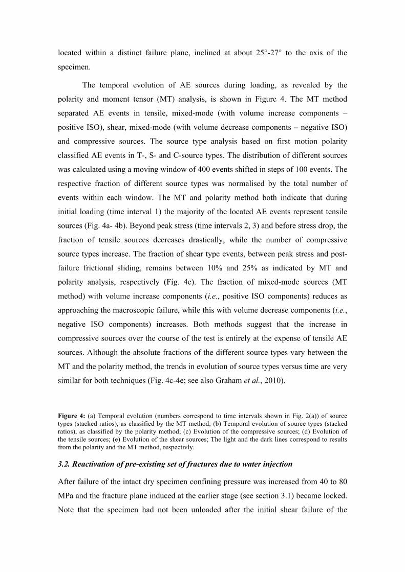
The temporal evolution of AE sources during loading, as revealed by the

polarity and moment tensor (MT) analysis, is shown in Figure 4. The MT method

separated AE events in tensile, mixed-mode (with volume increase components –

positive ISO), shear, mixed-mode (with volume decrease components – negative ISO)

and compressive sources. The source type analysis based on first motion polarity

classified AE events in T-, S- and C-source types. The distribution of different sources

was calculated using a moving window of 400 events shifted in steps of 100 events. The

respective fraction of different source types was normalised by the total number of

events within each window. The MT and polarity method both indicate that during

initial loading (time interval 1) the majority of the located AE events represent tensile

sources (Fig. 4a- 4b). Beyond peak stress (time intervals 2, 3) and before stress drop, the

fraction of tensile sources decreases drastically, while the number of compressive

source types increase. The fraction of shear type events, between peak stress and post-

failure frictional sliding, remains between 10% and 25% as indicated by MT and

polarity analysis, respectively (Fig. 4e). The fraction of mixed-mode sources (MT

method) with volume increase components (i.e., positive ISO components) reduces as

approaching the macroscopic failure, while this with volume decrease components (i.e.,

negative ISO components) increases. Both methods suggest that the increase in

compressive sources over the course of the test is entirely at the expense of tensile AE

sources. Although the absolute fractions of the different source types vary between the

MT and the polarity method, the trends in evolution of source types versus time are very

similar for both techniques (Fig. 4c-4e; see also Graham et al., 2010).

Figure 4: (a) Temporal evolution (numbers correspond to time intervals shown in Fig. 2(a)) of source types (stacked ratios), as classified by the MT method; (b) Temporal evolution of source types (stacked ratios), as classified by the polarity method; (c) Evolution of the compressive sources; (d) Evolution of the tensile sources; (e) Evolution of the shear sources; The light and the dark lines correspond to results from the polarity and the MT method, respectivly.

3.2. Reactivation of pre-existing set of fractures due to water injection

After failure of the intact dry specimen confining pressure was increased from 40 to 80

MPa and the fracture plane induced at the earlier stage (see section 3.1) became locked.

Note that the specimen had not been unloaded after the initial shear failure of the

previous loading stage (see section 3.1), to avoid potential further AE nucleation in

places of local stress concentration during the unloading stage (Charalampidou et al.,

2013). Subsequently, the Flechtingen sandstone specimen was loaded in triaxial

compression (at 80 MPa confining pressure) at a constant displacement rate of 20

µm/min. Axial loading was then stopped close to the peak stress (Fig. 5a, time interval

1). This stress value was defined after the onset of the non-linearity of the strain-stress

relation (not shown here) and the increase in the AE activity (Fig. 5a). The position of

the loading piston was kept constant for a few seconds (Fig. 5a, time interval 2) during

which the sample relaxed. Then constant axial force control was applied to the dry

specimen (Fig. 5a, time interval 3) and distilled water was injected into it through the

bottom port applying a constant inlet pore pressure of 5 MPa (Fig. 5a, time interval 4).

Before and after pore pressure stabilised at the pore fluid inlet (Fig. 5a, time intervals 4

and 5-9, respectively), axial force was held constant during the remainder of the water

injection. AE activity increased substantially just prior and during the failure induced

fluid injection. Fracture plane slip (452 µm axial shortening) was associated with a

significant stress drop (63.7 MPa, Fig. 5a, time interval 9). After the slip event the

position of the piston was held constant temporarily (Fig. 5a, time interval 10) before

again subjecting the sample to the pre-failure displacement rate of 20 µm/min (Fig. 5a,

time interval 11). In a final step the position of the piston was held constant and the

specimen was allowed to creep for a longer period (Fig. 5a, time interval 12) while

becoming fully saturated (as velocity evolution shows in Fig. 5c).

Differential stress and cumulative AE number increase with increasing time

when the specimen is loaded at a constant displacement rate. Since we switched to

constant axial force control during injection, the AE activity slowed down (Fig. 5a, time

intervals 3-6). However, just prior to macroscopic failure AE activity increased

exponentially (Fig. 5, time intervals 7-9). The axial shortening increased from 163 µm

during the pre-failure steps (Fig. 5b, between time intervals 7 and 8) to 452 µm (Fig. 5b,

in time interval 9) during the stress drop. Pore pressure showed a small pressure drop of

about 0.1 MPa at failure (Fig. 5b, time interval 9). With onset of pore fluid injection, P-

wave velocities recorded in the vertical direction increase slowly. Nonetheless,

progressive saturation of the sample is indicated by significant increase of horizontal

velocities. Irrespective of the presence of a shear fracture cutting across the specimen

(Fig. 5d, time interval 9), the rise of the water front occurs across the entire specimen

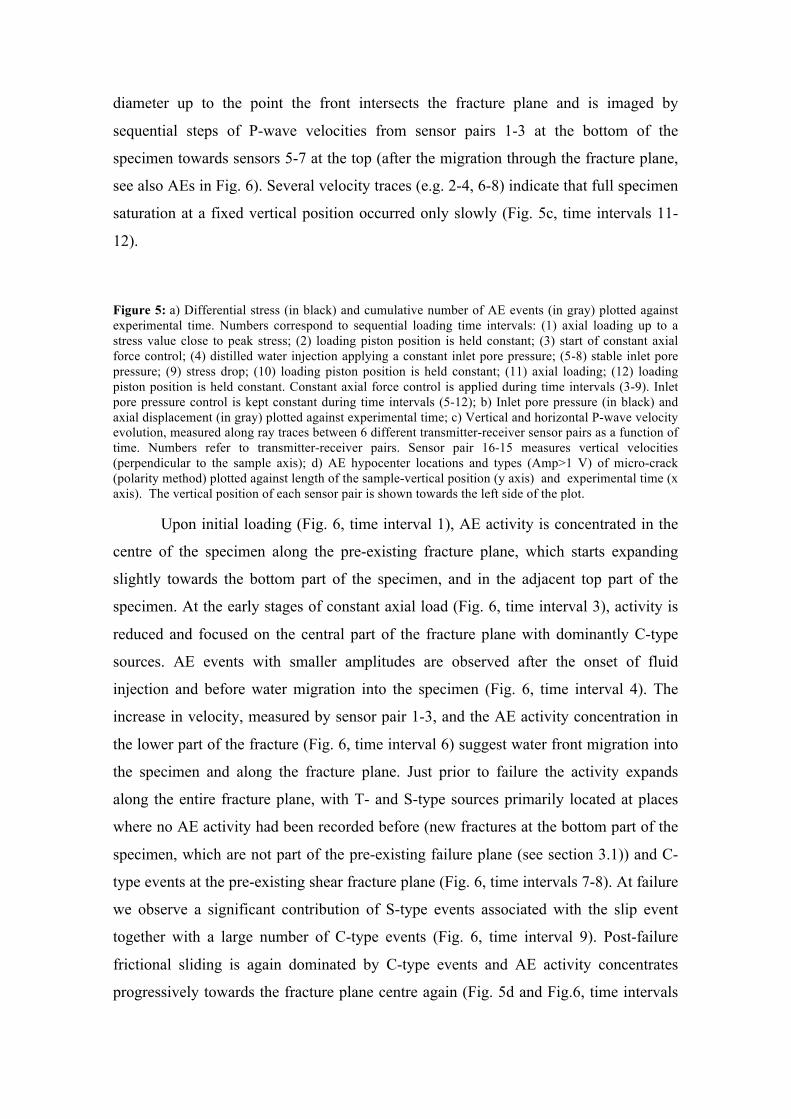
diameter up to the point the front intersects the fracture plane and is imaged by

sequential steps of P-wave velocities from sensor pairs 1-3 at the bottom of the

specimen towards sensors 5-7 at the top (after the migration through the fracture plane,

see also AEs in Fig. 6). Several velocity traces (e.g. 2-4, 6-8) indicate that full specimen

saturation at a fixed vertical position occurred only slowly (Fig. 5c, time intervals 11-

12).

Figure 5:  a) Differential stress (in black) and cumulative number of AE events (in gray) plotted against experimental time. Numbers correspond to sequential loading time intervals: (1) axial loading up to a stress value close to peak stress; (2) loading piston position is held constant; (3) start of constant axial force control; (4) distilled water injection applying a constant inlet pore pressure; (5-8) stable inlet pore pressure; (9) stress drop; (10) loading piston position is held constant; (11) axial loading; (12) loading piston position is held constant. Constant axial force control is applied during time intervals (3-9). Inlet pore pressure control is kept constant during time intervals (5-12); b) Inlet pore pressure (in black) and axial displacement (in gray) plotted against experimental time; c) Vertical and horizontal P-wave velocity evolution, measured along ray traces between 6 different transmitter-receiver sensor pairs as a function of time. Numbers refer to transmitter-receiver pairs. Sensor pair 16-15 measures vertical velocities (perpendicular to the sample axis); d) AE hypocenter locations and types (Amp>1 V) of micro-crack (polarity method) plotted against length of the sample-vertical position (y axis) and experimental time (x axis). The vertical position of each sensor pair is shown towards the left side of the plot.  

Upon initial loading (Fig. 6, time interval 1), AE activity is concentrated in the

centre of the specimen along the pre-existing fracture plane, which starts expanding

slightly towards the bottom part of the specimen, and in the adjacent top part of the

specimen. At the early stages of constant axial load (Fig. 6, time interval 3), activity is

reduced and focused on the central part of the fracture plane with dominantly C-type

sources. AE events with smaller amplitudes are observed after the onset of fluid

injection and before water migration into the specimen (Fig. 6, time interval 4). The

increase in velocity, measured by sensor pair 1-3, and the AE activity concentration in

the lower part of the fracture (Fig. 6, time interval 6) suggest water front migration into

the specimen and along the fracture plane. Just prior to failure the activity expands

along the entire fracture plane, with T- and S-type sources primarily located at places

where no AE activity had been recorded before (new fractures at the bottom part of the

specimen, which are not part of the pre-existing failure plane (see section 3.1)) and C-

type events at the pre-existing shear fracture plane (Fig. 6, time intervals 7-8). At failure

we observe a significant contribution of S-type events associated with the slip event

together with a large number of C-type events (Fig. 6, time interval 9). Post-failure

frictional sliding is again dominated by C-type events and AE activity concentrates

progressively towards the fracture plane centre again (Fig. 5d and Fig.6, time intervals

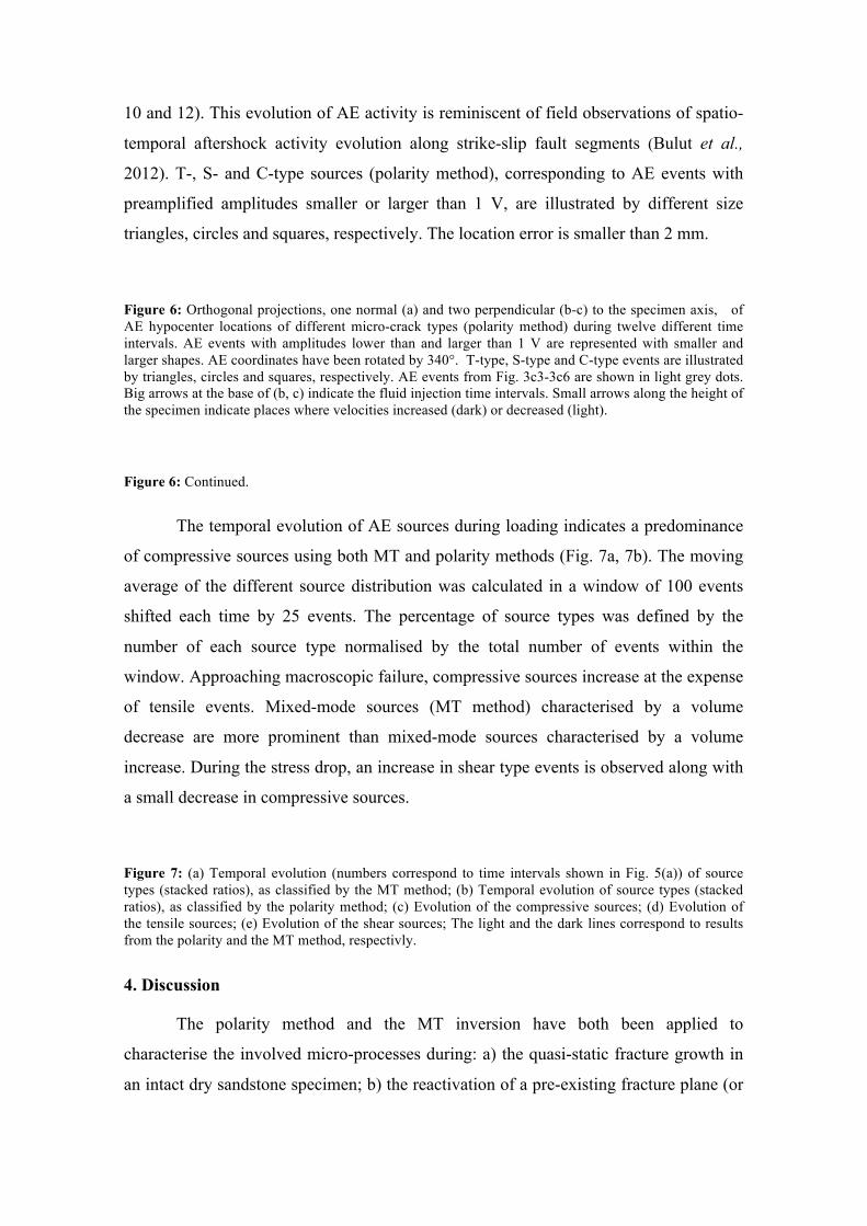
10 and 12). This evolution of AE activity is reminiscent of field observations of spatio-

temporal aftershock activity evolution along strike-slip fault segments (Bulut et al.,

2012). T-, S- and C-type sources (polarity method), corresponding to AE events with

preamplified amplitudes smaller or larger than 1 V, are illustrated by different size

triangles, circles and squares, respectively. The location error is smaller than 2 mm.

Figure 6: Orthogonal projections, one normal (a) and two perpendicular (b-c) to the specimen axis, of AE hypocenter locations of different micro-crack types (polarity method) during twelve different time intervals. AE events with amplitudes lower than and larger than 1 V are represented with smaller and larger shapes. AE coordinates have been rotated by 340°. T-type, S-type and C-type events are illustrated by triangles, circles and squares, respectively. AE events from Fig. 3c3-3c6 are shown in light grey dots. Big arrows at the base of (b, c) indicate the fluid injection time intervals. Small arrows along the height of the specimen indicate places where velocities increased (dark) or decreased (light).

Figure 6: Continued.

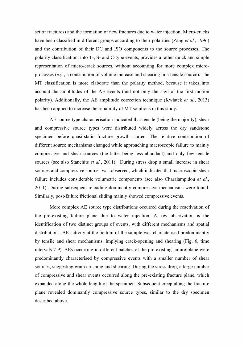
The temporal evolution of AE sources during loading indicates a predominance

of compressive sources using both MT and polarity methods (Fig. 7a, 7b). The moving

average of the different source distribution was calculated in a window of 100 events

shifted each time by 25 events. The percentage of source types was defined by the

number of each source type normalised by the total number of events within the

window. Approaching macroscopic failure, compressive sources increase at the expense

of tensile events. Mixed-mode sources (MT method) characterised by a volume

decrease are more prominent than mixed-mode sources characterised by a volume

increase. During the stress drop, an increase in shear type events is observed along with

a small decrease in compressive sources.

Figure 7: (a) Temporal evolution (numbers correspond to time intervals shown in Fig. 5(a)) of source types (stacked ratios), as classified by the MT method; (b) Temporal evolution of source types (stacked ratios), as classified by the polarity method; (c) Evolution of the compressive sources; (d) Evolution of the tensile sources; (e) Evolution of the shear sources; The light and the dark lines correspond to results from the polarity and the MT method, respectivly.  

4. Discussion

The polarity method and the MT inversion have both been applied to

characterise the involved micro-processes during: a) the quasi-static fracture growth in

an intact dry sandstone specimen; b) the reactivation of a pre-existing fracture plane (or

set of fractures) and the formation of new fractures due to water injection. Micro-cracks

have been classified in different groups according to their polarities (Zang et al., 1996)

and the contribution of their DC and ISO components to the source processes. The

polarity classification, into T-, S- and C-type events, provides a rather quick and simple

representation of micro-crack sources, without accounting for more complex micro-

processes (e.g., a contribution of volume increase and shearing in a tensile source). The

MT classification is more elaborate than the polarity method, because it takes into

account the amplitudes of the AE events (and not only the sign of the first motion

polarity). Additionally, the AE amplitude correction technique (Kwiatek et al., 2013)

has been applied to increase the reliability of MT solutions in this study.

AE source type characterisation indicated that tensile (being the majority), shear

and compressive source types were distributed widely across the dry sandstone

specimen before quasi-static fracture growth started. The relative contribution of

different source mechanisms changed while approaching macroscopic failure to mainly

compressive and shear sources (the latter being less abundant) and only few tensile

sources (see also Stanchits et al., 2011). During stress drop a small increase in shear

sources and compressive sources was observed, which indicates that macroscopic shear

failure includes considerable volumetric components (see also Charalampidou et al.,

2011). During subsequent reloading dominantly compressive mechanisms were found.

Similarly, post-failure frictional sliding mainly showed compressive events.

More complex AE source type distributions occurred during the reactivation of

the pre-existing failure plane due to water injection. A key observation is the

identification of two distinct groups of events, with different mechanisms and spatial

distributions. AE activity at the bottom of the sample was characterised predominantly

by tensile and shear mechanisms, implying crack-opening and shearing (Fig. 6, time

intervals 7-9). AEs occurring in different patches of the pre-existing failure plane were

predominantly characterised by compressive events with a smaller number of shear

sources, suggesting grain crushing and shearing. During the stress drop, a large number

of compressive and shear events occurred along the pre-existing fracture plane, which

expanded along the whole length of the specimen. Subsequent creep along the fracture

plane revealed dominantly compressive source types, similar to the dry specimen

described above.

Since the sandstone was previously subjected to elevated stresses close to peak

stress, fluid migration likely caused a local decrease in effective stresses, leading to

macroscopic failure. Variations in elastic wave velocities have been used to monitor

water migration (see also Masuda et al., 1993; Stanchits et al., 2011) and damage (see

Fortin et al., 2005) inside the pre-fractured sandstone specimen. A considerable increase

in velocities of sensor pair 1-3 indicated water infiltration inside the specimen up to the

position of these sensors. Subsequent smaller velocity increase may be related to water

progressively filling pore space along the pre-existing failure plane. During sliding and

fluid induced reactivation of the shear fracture we mainly observed compression events.

The observed channelling of the injected fluid into the fracture plane suggests that

irrespective of compaction along the fracture plane its permeability remained high

compared to the intact sandstone walls. This is in accordance with results from post-

deformation fluid flow monitoring (unconfined) via neutron radiography in another

sandstone, containing a compactant shear band (Hall, 2013), where fluid migration

inside the shear band was faster than in the sandstone outside.

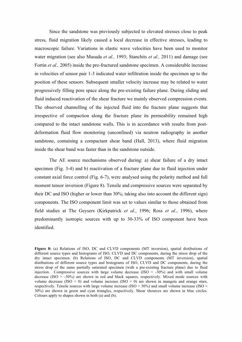
The AE source mechanisms observed during: a) shear failure of a dry intact

specimen (Fig. 3-4) and b) reactivation of a fracture plane due to fluid injection under

constant axial force control (Fig. 6-7), were analysed using the polarity method and full

moment tensor inversion (Figure 8). Tensile and compressive sources were separated by

their DC and ISO (higher or lower than 30%; taking also into account the different sign)

components. The ISO component limit was set to values similar to those obtained from

field studies at The Geysers (Kirkpatrick et al., 1996; Ross et al., 1996), where

predominantly isotropic sources with up to 30-33% of ISO component have been

identified.

Figure 8: (a) Relations of ISO, DC and CLVD components (MT inversion), spatial distibutions of different source types and histograms of ISO, CLVD and DC components, during the stress drop of the dry intact specimen. (b) Relations of ISO, DC and CLVD components (MT inversion), spatial distibutions of different source types and histograms of ISO, CLVD and DC components, during the stress drop of the same partially saturated specimen (with a pre-existing fracture plane) due to fluid injection. Compressive sources with large volume decrease (ISO < -30%) and with small volume decrease (ISO > -30%) are shown in red and black squares, respectively. Mixed mode sources with volume decrease (ISO < 0) and volume increase (ISO > 0) are shown in mangeta and orange stars, respectively. Tensile sources with large volume increase (ISO > 30%) and small volume increase (ISO < 30%) are shown in green and cyan triangles, respectively. Shear shources are shown in blue circles. Colours apply to shapes shown in both (a) and (b).  

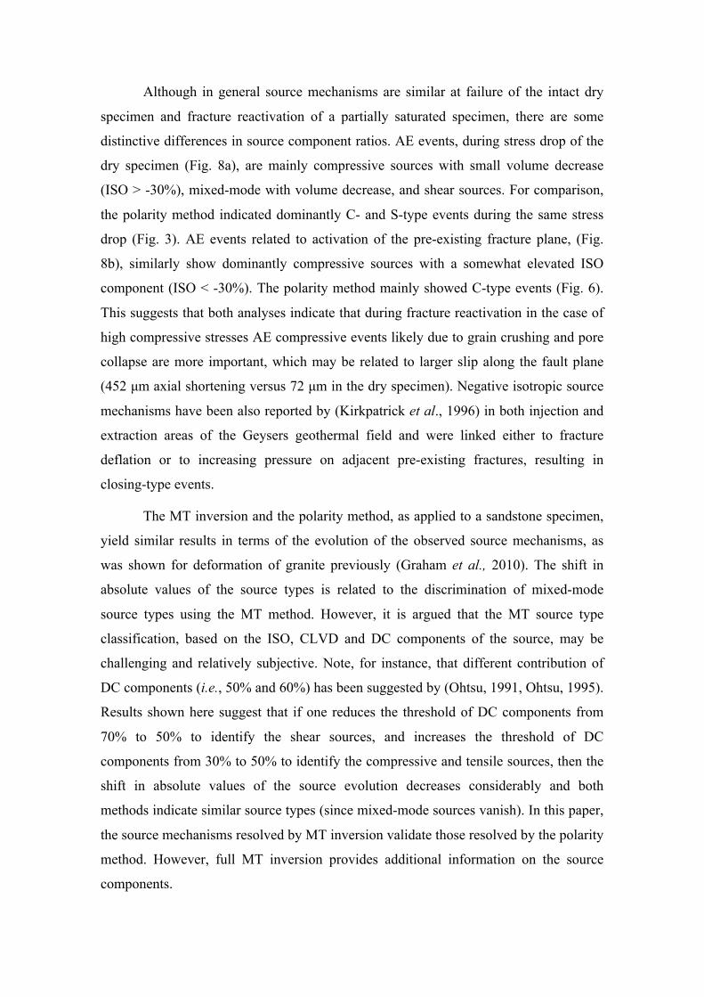
Although in general source mechanisms are similar at failure of the intact dry

specimen and fracture reactivation of a partially saturated specimen, there are some

distinctive differences in source component ratios. AE events, during stress drop of the

dry specimen (Fig. 8a), are mainly compressive sources with small volume decrease

(ISO > -30%), mixed-mode with volume decrease, and shear sources. For comparison,

the polarity method indicated dominantly C- and S-type events during the same stress

drop (Fig. 3). AE events related to activation of the pre-existing fracture plane, (Fig.

8b), similarly show dominantly compressive sources with a somewhat elevated ISO

component (ISO < -30%). The polarity method mainly showed C-type events (Fig. 6).

This suggests that both analyses indicate that during fracture reactivation in the case of

high compressive stresses AE compressive events likely due to grain crushing and pore

collapse are more important, which may be related to larger slip along the fault plane

(452 µm axial shortening versus 72 µm in the dry specimen). Negative isotropic source

mechanisms have been also reported by (Kirkpatrick et al., 1996) in both injection and

extraction areas of the Geysers geothermal field and were linked either to fracture

deflation or to increasing pressure on adjacent pre-existing fractures, resulting in

closing-type events.

The MT inversion and the polarity method, as applied to a sandstone specimen,

yield similar results in terms of the evolution of the observed source mechanisms, as

was shown for deformation of granite previously (Graham et al., 2010). The shift in

absolute values of the source types is related to the discrimination of mixed-mode

source types using the MT method. However, it is argued that the MT source type

classification, based on the ISO, CLVD and DC components of the source, may be

challenging and relatively subjective. Note, for instance, that different contribution of

DC components (i.e., 50% and 60%) has been suggested by (Ohtsu, 1991, Ohtsu, 1995).

Results shown here suggest that if one reduces the threshold of DC components from

70% to 50% to identify the shear sources, and increases the threshold of DC

components from 30% to 50% to identify the compressive and tensile sources, then the

shift in absolute values of the source evolution decreases considerably and both

methods indicate similar source types (since mixed-mode sources vanish). In this paper,

the source mechanisms resolved by MT inversion validate those resolved by the polarity

method. However, full MT inversion provides additional information on the source

components.

5. Conclusions

Shear failure in a dry intact sandstone specimen, when subjected to brittle conditions,

involves mainly compressive and shear mechanisms. Reactivation of a pre-existing

shear failure plane, using constant axial load when subjected to elevated stresses, due to

water injection is expressed primarily via compression and shearing along the pre-

existing shear fracture plane and via dilation and shearing along the newly created

fractures in places far from the pre-existing failure plane. The reactivation due to water

injection promoted compressive sources along the pre-existing failure plane with higher

volumetric components than the equivalent compressive sources during the fracturing of

the dry intact specimen. Ultrasonic velocity measurements could capture water (and

pore fluid) migration inside an initially dry specimen. The observed channelling of the

injected fluid into the pre-existing fracture plane indicates that despite compaction along

the failure plane, its permeability remains higher than that of the sandstone matrix. To

analyse the source mechanisms of AE activity during sample deformation we employed

the polarity method and the full MT inversion. Both techniques reveal similar

mechanisms; however, the MT inversion provided more information on the source

components.

Acknowledgments

The authors would like to particularly thank Stefan Gehrmann (GFZ) for the specimen preparation. Helen Lewis, Antonio Claudio Soares and two more anonymous reviewers are gratefully acknowledged for their fruitful comments. This work has been funded by the EU-GEISER Project (FP7-ENERGY-2009).

Bibliography:

1. Bulut, F., Bohnhoff, M., Eken, T., Janssen, C., Kilic, T., Dresen, G. (2012). The East Anatolian Fault Zone: Seismotectonic setting and spatiotemporal characteristics of seismocity based on precese earthquake locations. J. Geophys. Res., 117, B07304, doi: 10.1029/2011JB008966.

2. Charalampidou, E.M., Hall, S.A., Stanchits, S., Lewis, H., Viggiani, G. (2011). Characterization of shear and compaction bands in a porous sandstone deformed under triaxial compression. Tectonophysics, 503, 1-2, 8-17.

3. Charalampidou, E.M., Hall, S.A., Stanchits, S., Viggiani, G., Lewis, H. (2013). Shear-enhanced compaction band identification at the laboratory scale using acoustic and full-field methods. Int. J. Rock Mech. Min. Sci., doi:10.1016/j.ijrmms.2013.05.006.

4. Cuenot, N., Dorbath, C., Dorbath, L. (2008). Analysis of Microseismicity Induced by Fluid Injections at the EGS Site of Soultz-sous-foret (Alsace, France): Implications for the Characterisation of the Geothermal Reservoir Properties. Pure and Applied Geophysics, 165, 797-828.

5. Ellenberg, J., Falk, F., Grumbt, E., Lutzner. H., Ludwig, O. (1976). Sedimentation des höheren Unterperms der Flechtinger Scholle. Z. Geol. Wiss., 4, 705-737.

6. Evans K. F., Zappone, A., Kraft, T., Deichmann, N., Moia, F. (2012). A survey of the induced seismic responses to fluid injection in geothermal and CO2 reservoirs in Europe. Geothermics, 41, 30-54.

7. Fortin, J., Schubnel, A., Gueguen, Y. (2005). Elastic wave velocities and permeability evolution during compaction of Bleurswiller sandstone. Int. J. Rock Mech. Min. Sci., 42, 873-889.

8. Giardini, D. (2009). Geothermal quake risks must be faced. Nature, 462, 848-849, doi: 10.1038/462848a.

9. Graham C.C., Stanchits S., Main I.G., Dresen G. (2010). Comparison of polarity and moment tensor inversion methods for source analysis of acoustic emission data. Int. J. Rock Mech. Min. Sci., 47, 161-169.

10. Hall, S.A. (2013). Characterisation of fluid flow in a shear-band in porous rock using neutron radiography. GRL, doi: 10.1002/grl.50528.

11. Holland, A.A. (2013). Earthquakes Triggered by Hydraulic Fracturing in South‐Central Oklahoma. Bulletin of the Seismological Society of America, 103, 3, 1784-1792.

12. Kirkpatrick, A., Peterson, J.E., Majer. J., Majer, E.L. (1996, January). Source Mechanisms of Microerthquakes at the southeast Geysers geothermal field, California. Paper presented at the 21st Workshop on geothermal reservoir engineering, Stanford University, Standford, California.

13. Kwiatek, G., Charalampidou, E.M., Dresen, G., Stanchits, S. An improved method for seismic moment tensor inversion of acoustic emissions through assessment of sensor coupling and sensitivity to incident angle. Int. J. Rock Mech. Min. Sci., (in press, http://dx.doi.org/10.1016/j.ijrmms.2013.11.005).

14. Leonard M. and Kennett B.L.N. (1999). Multi-component autoregressive techniques for the analysis of seismograms. Phys. Earth Planet. Int.,113 (1-4), 247.

15. Lockner, D.A., Byerlee, J.D., Kuksenko, V., Ponomarev, A., Sidorin, A. (1991). Quasi-static fault growth and shear fracture energy in granite. Nature, 350, 39-42.

16. Lockner, D.A., Byerlee, J.D., Kuksenko, V., Ponomarev, A., Sidorin, A. (1992). Observation of quasistatic fault growth from acoustic emissions. In B. Evans, T.-F. Wong (Ed.), Fault mechanics and transport properties of rocks (pp. 3-31). London: Academic Press.

17. Majer, E. L., Peterson, J. (2007). The impact of injection on the seismicity at The Geysers, California Geothermal Field. Int. J. Rock Mech. Min. Sci., 44, 1079-1090.

18. Majer, E. L., Baria, R., Stark, M., Oates, S., Bommer, J., Smith, B., Asanuma, H. (2007). Induced seismicity associated with Enhanced Geothermal Systems. Geothermics, 36, 185-222.

19. Masuda, K., Nishizawa, O., Kusunose, K., Satoh, T. (1993). Laboratory study of Effects of In situ Stress State and Strength on Fluid-Induced Seismicity. Int. J. Rock Mech. Min. Sci. & Geomech. Abstr., 30, 1, 1-10.

20. Mayr, S.I., Stanchits, S., Langenbruch, C., Dresen, G., Shapiro, S. (2011). Acoustic emission induced by pore-pressure changes in sandstone samples. Geophysics, 76, 3.

21. Nelder J. and Mead R. (1965). A simplex method for function minimization. Computer J., 7, 308-312.

22. Ohtsu, M. (1991). Simplified Moment Tensor Analysis and Unified Decomposition of Acoustic Emission Source: Application to in Situ Hydrofracturing Test. J. Geophys. Res., 96, B4, 6211-6221.

23. Ohtsu, M. (1995). Acoustic Emission theory for Moment Tensor Analysis. Res. Nondestr. Eval., 6 :169-184.

24. Ross, A., Foulger, G.R., Julian, B.R. (1996). Non double-couple earthquake mechanisms at the Geysers geothermal area, California. Geophys. Res. Lett., 23, 8, 877-880.

25. Stanchits S., Dresen G. and Vinciguerra S. (2006). Ultrasonic velocities, acoustic emission characteristics and crack damage of basalt and granite. Pure Appl. Geophys., 163, 5–6, 975–994.

26. Stanchits S., Fortin J., Guéguen Y., Dresen G. (2009). Initiation and Propagation of Compaction Bands in Dry and Wet Bentheim Sandstone. Pure Appl. Geophys., 166, 843-868.

27. Stanchits, S., Mayr, S., Shapiro, S., Dresen, G. (2011). Fracturing of porous rock induced by fluid injection. Tectonophysics, 503, 129-145.

28. Tezuka, K., Niitsuma, H. (2000). Stress estimated using microseismic clusters and its relationship to the fracture systems of the Hijiori hot dry rock reservoir. Engineering Geology, 56, 47-62.

29. Vavrycuk, V. (2001). Inversion for parametwers of tensile earthquakes. J. Geophys. Res.,106, B8, 16339-16355.

30. Zang, A., Wagner, C.F., Dresen, G. (1996). Acoustic emission, microstructure, and damage model of dry and wet sandstone stressed to failure. J. Geophys. Res., 101, B8, 17507-17521.

31. Zang A., Wagner F.C., Stanchits S., Dresen G., Andresen R., Haidekker M.A. (1998). Source analysis of acoustic emissions in Aue granite cores under symmetric and asymmetric compressive loads. Geophys. J., Int., 135, 1113-1130.

32. Zoback, M., Harjes, H.P. (1997). Injection-induced earthquakes and crustal stress at 9 km depth at the KTB deep drilling site, Germany. J. Geophys. Res., 102 (B8), 18477-18491. Figures Figure 1: a) Schematic view of the specimen geometry, showing the positions of the P-

wave sensors; b) Map of the azimuthial coverage of P-wave sensors used as receivers

and transmitters (in light bold colours) and as receivers (in dark bold colours) during the

experiment.  

Figure 2: a) Differential stress and cumulative number of AE events plotted against

experimental time. Numbers correspond to sequential loading time intervals: (1) up to

the peak stress; (2 and 3) during the post-peak stress; (4), during the stress drop; (5)

during the reloading; and (6) during the time that the position of the loading piston was

fixed; b) Vertical and horizontal P-wave velocity evolution, measured along ray traces

between 6 different transmitter-receiver sensor pairs, as a function of time. Numbers

refer to transmitter-receiver pairs. Sensor pair 16-15 measures vertical velocities

(perpendicular to the sample axis); c) AE hypocenter locations and types (Amp>1 V) of

micro-cracks (polarity method) plotted against length of the sample-vertical position (y

axis) and experimental time (x axis). The vertical position of each sensor pair is

shown towards the left side of the plot.  

Figure 3: Orthogonal projections, one normal (a) and two perpendicular (b-c) to the

specimen axis, of AE hypocenter locations showing different micro-crack types

(polarity method) during six different time intervals (steps 1-6: see figure 2(a)). T-type,

S-type and C-type events are illustrated by triangles, circles and squares, repsectively.

AE events have amplitudes larger than 1 V and AE coordinates have been rotated by

340° so as to have a better view of the fracture plane.  

Figure 4: (a) Temporal evolution (numbers correspond to time intervals shown in Fig.

2(a)) of source types (stacked ratios), as classified by the MT method; (b) Temporal

evolution of source types (stacked ratios), as classified by the polarity method; (c)

Evolution of the compressive sources; (d) Evolution of the tensile sources; (e) Evolution

of the shear sources; The light and the dark lines correspond to results from the polarity

and the MT method, respectivly.  

Figure 5: a) Differential stress (in black) and cumulative number of AE events (in gray)

plotted against experimental time. Numbers correspond to sequential loading time

intervals: (1) axial loading up to a stress value close to peak stress; (2) loading piston

position is held constant; (3) start of constant axial force control; (4) distilled water

injection applying a constant inlet pore pressure; (5-8) stable inlet pore pressure; (9)

stress drop; (10) loading piston position is held constant; (11) axial loading; (12)

loading piston position is held constant. Constant axial force control is applied during

time intervals (3-9). Inlet pore pressure control is kept constant during time intervals (5-

12); b) Inlet pore pressure (in black) and axial displacement (in gray) plotted against

experimental time; c) Vertical and horizontal P-wave velocity evolution, measured

along ray traces between 6 different transmitter-receiver sensor pairs as a function of

time. Numbers refer to transmitter-receiver pairs. Sensor pair 16-15 measures vertical

velocities (perpendicular to the sample axis); d) AE hypocenter locations and types

(Amp>1 V) of micro-crack (polarity method) plotted against length of the sample-

vertical position (y axis) and experimental time (x axis). The vertical position of each

sensor pair is shown towards the left side of the plot.  

Figure 6: Orthogonal projections, one normal (a) and two perpendicular (b-c) to the

specimen axis, of AE hypocenter locations of different micro-crack types (polarity

method) during twelve different time intervals. AE events with amplitudes lower than

and larger than 1 V are represented with smaller and larger shapes. AE coordinates have

been rotated by 340°. T-type, S-type and C-type events are illustrated by triangles,

circles and squares, respectively. AE events from Fig. 3c3-3c6 are shown in light grey

dots. Big arrows at the base of (b, c) indicate the fluid injection time intervals. Small

arrows along the height of the specimen indicate places where velocities increased

(dark) or decreased (light).  

Figure 7: (a) Temporal evolution (numbers correspond to time intervals shown in Fig.

5(a)) of source types (stacked ratios), as classified by the MT method; (b) Temporal

evolution of source types (stacked ratios), as classified by the polarity method; (c)

Evolution of the compressive sources; (d) Evolution of the tensile sources; (e) Evolution

of the shear sources; The light and the dark lines correspond to results from the polarity

and the MT method, respectivly.  

Figure 8: (a) Relations of ISO, DC and CLVD components (MT inversion), spatial

distibutions of different source types and histograms of ISO, CLVD and DC

components, during the stress drop of the dry intact specimen. (b) Relations of ISO, DC

and CLVD components (MT inversion), spatial distibutions of different source types

and histograms of ISO, CLVD and DC components, during the stress drop of the same

partially saturated specimen (with a pre-existing fracture plane) due to fluid injection.

Compressive sources with large volume decrease (ISO < -30%) and with small volume

decrease (ISO > -30%) are shown in red and black squares, respectively. Mixed mode

sources with volume decrease (ISO < 0) and volume increase (ISO > 0) are shown in

mangeta and orange stars, respectively. Tensile sources with large volume increase (ISO

> 30%) and small volume increase (ISO < 30%) are shown in green and cyan triangles,

respectively. Shear shources are shown in blue circles. Colours apply to shapes shown

in both (a) and (b).  

 Fig.1  

 Fig.  2  

 Fig.  3  

 Fig.  4  

 Fig.  5  

 

 Fig.  6  

 Fig.  7  

 Fig.  8