Embed Size (px)
Citation preview

WI-
339
University of Augsburg, D-86135 Augsburg Visitors: Universitätsstr. 12, 86159 Augsburg Phone: +49 821 598-4801 (Fax: -4899) University of Bayreuth, D-95440 Bayreuth Visitors: F.-v.-Schiller-Str. 2a, 95444 Bayreuth Phone: +49 921 55-4710 (Fax: -844710) www.fim-rc.de
Discussion Paper
Bringing value-based Business Process Management to the Operational Process Level
by
Manuel Bolsinger1
1 At the time of writing this paper, Manuel Bolsinger was a research assistant at the Research Center Finance & Information Management and the Department of Information Systems Engineering & Financial Management at the University of Augsburg.
in: Information Systems and e-Business Management, 13, 2, 2015, p. 355-398
The final publication is available at Springer via http://dx.doi.org/10.1007/s10257-014-0248-1

1
Bringing value-based business process management to the operational process level1
Manuel Bolsinger
Bolsinger, Manuel, Research Center Finance & Information Management, University of
Augsburg, Universitaetsstrasse 12, 86159 Augsburg, Germany,
[email protected], +49 821 – 598 4885 (phone), +49 821 – 598 4899 (fax)
Abstract
For years, improving processes has been a prominent business priority for Chief Information
Officers. As expressed by the popular saying, “If you can’t measure it, you can’t manage it,”
process measures are an important instrument for managing processes and corresponding
change projects. Companies have been using a value-based management approach since the
1990s in a constant endeavor to increase their value. Value-based business process management
introduces value-based management principles to business process management and uses a risk-
adjusted expected net present value as the process measure. However, existing analyses of this
issue operate at a high (i.e., corporate) level, hampering the use of value-based business process
management at an operational process level in both research and practice. Therefore, this paper
proposes a valuation calculus that brings value-based business process management to the
operational process level by showing how the risk-adjusted expected net present value of a
process can be determined. We demonstrate that the valuation calculus provides insights into
the theoretical foundations of processes and helps improve the calculation capabilities of an
existing process-modeling tool.
Keywords: Value-Based Business Process management; Process Modeling; Process Measure;
Net Present Value; Certainty Equivalent; Expected Value; Variance
1 Grateful acknowledgement is due to the DFG (German Research Foundation) for their support of the projects “Modeling,
self-composition and self-configuration of reference processes based on semantic concepts (SEMPRO²)” (BU 809/7-2) and
“Integrated Enterprise Balancing (IEB)” (BU 809/8-1) making this paper possible.
2
1 Introduction
Constant change in their economic, political, and social environments is forcing companies to
strive for increased efficiency and more frequent innovation (Becker and Kahn 2005, p. 3), a
situation in which the management and, in particular, the improvement of processes play a
considerable role (González et al. 2010; Thome et al. 2011; van der Aalst 2013; vom Brocke et
al. 2011a). One indicator of process improvement’s prominent role is the fact that companies
invest considerable amounts of money to develop their business process management (BPM)
capabilities and realize improvement activities (Wolf and Harmon 2012). The volume of
research on process improvement has also increased (Sidorova and Isik 2010, p. 572).
In their efforts to improve processes, researchers and practitioners alike must establish a basis
on which it can be decided that an alternative (or “to-be”) process is better than an existing (or
“as-is”) process. The instruments deemed appropriate for determining the extent to which a
process alternative improves an existing process are called “process measures” (González et al.
2010; Tregear 2012; zur Muehlen and Shapiro 2010). When the value of a process measure of
an alternative process is greater than that of an existing process, it might be reasonable to
implement the alternative process and thus improve the existing process. However, there are
many process measures, and, while the value of one measure may suggest a process
improvement, the value of another may indicate the opposite. For example, the dimensions of
time, cost, quality, and flexibility, often used to evaluate process improvement, comprise the
so-called “devil’s quadrangle” because, “in general, improving [a process] upon one dimension
may have a weakening effect on another” (Reijers and Liman Mansar 2005, p. 294). Hence,
process managers have to consider these complementary and competitive goal relations when
determining whether an alternative process improves an existing process. In order to resolve
potential conflicts among goals, process managers need integrated approaches that consolidate
various goals into one overall goal, thus allowing them to make decisions based on that overall
goal.
Value-based BPM introduces into BPM an overall goal in line with economic theory (Buhl et
al. 2011). Value-based BPM applies value-based management principles to process decision-
making and aims to increase company value from a long-term perspective (Ittner and Larcker
2001; Koller et al. 2010; Young and O'Byrne 2001), thus supporting process improvement from
a monetary-centered view of BPM. Companies have been using value-based management since
the 1990s in their constant endeavor to increase their value (Coenenberg and Salfeld 2007, p.
3). Almost two thirds of the 30 companies on the German stock index (DAX), representing
Germany’s major companies, explicitly state in their 2013 annual reports that they follow a
value-based management approach. Moreover, the 2013 CIO agenda (Gartner 2013) identified
“harvest value from business process changes” as one of their three performance profiles.
Hence, value-based BPM not only provides an approach for integrating different goals but also
takes on a business perspective by facilitating the overall goal of increasing company value,
wherein a process’ value contribution is determined by its risk-adjusted expected net present
value, or “rNPV” (Bolsinger et al. 2011; Buhl et al. 2011). A process alternative should be
implemented as an improvement whenever its rNPV is higher than that of the existing process.
However, although research suggests the transferability of value-based management to BPM,
current studies operate at a high (i.e., corporate) level and do not show how the rNPV is to be
calculated in detail, particularly with reference to a process’ control flow, which is important to
connect the corporate level with the operational level (Rotaru et al. 2011; vom Brocke et al.
2010). Furthermore, in the practice of BPM, modeling tools (e.g., IBM WebSphere Business

3
Modeler Advanced, Bonita Studio, TIBCO Business Studio, ibo Prometheus Klassik and Bizz
Designer) cannot determine the rNPV and, thus, do not support value-based BPM. In order to
substantiate value-based BPM from both theoretical and practical points of view, additional
research capable of establishing the appropriate theoretical foundations is necessary (Vergidis
et al. 2008).
This paper contributes to the literature by providing a valuation calculus for determining the
risk-adjusted expected net present value of a process. After the valuation calculus is
implemented, a process-modeling tool could calculate the rNPV for various process
alternatives, from which a process manager could choose for a process improvement project.
This functionality would provide a valuable asset for process managers (van Hee and Reijers
2000; Vergidis et al. 2008) and bring value-based management into the practice of BPM.
This paper, reflecting the design science research process presented in Peffers et al. (2008), is
organized as follows. After motivating the importance of the problem in this section, Section 2
provides more background information about value-based BPM and positions it against other
BPM approaches related to value-based BPM. Based on this theoretical background, we derive
the requirements for the valuation calculus that define its objectives before discussing related
work. In Section 3, we introduce a basic illustrative example to provide a better understanding
of the issues raised in the subsequent sections. In Section 4, the valuation calculus (our artifact)
is designed using a formal-deductive research approach (Meredith et al. 1989). In Section 5, we
focus on the evaluation of the valuation calculus in an artificial setting (Sonnenberg and vom
Brocke 2012; Venable et al. 2012). We then present a feature comparison, a comparison with a
related artifact, and a demonstration of the feasibility of the artifact by solving an exemplary
problem instance and by illustrating how the knowledge of the valuation calculus corrected the
calculation logic of the process-modeling tool of the CubeFour company. Finally, the last
section summarizes our results and provides an outlook for future study.
2 Theoretical Background
2.1 Value-based Business Process Management
The value-based BPM paradigm focuses on the value that a newly designed process or a change
in an existing process contributes to a company (Buhl et al. 2011; vom Brocke et al. 2010). In
doing so, value-based BPM introduces value-based management principles to BPM, thus
motivating process-related decisions according to a well-established management approach.
Before discussing value-based BPM in detail, we will first outline the principles of value-based
management.
Value-based management aims to sustainably increase a company’s value from a long-term
perspective (Ittner and Larcker 2001; Koller et al. 2010; Young and O'Byrne 2001). It extends
the shareholder value approach that traces back to Rappaport (1986) and was further advanced
by Copeland et al. (1990) and Stewart and Stern (1991). Taking a long-term perspective, value-
based management complies with the stakeholder value approach (Danielson et al. 2008), which
is important for a less decision-making oriented perspective on value-based BPM (vom Brocke
et al. 2009). For value-based management to be fully realized, all activities on all company
levels must be aligned with the goal of maximizing company value (Coenenberg and Salfeld
2007). The same holds true for company processes: each process has to contribute to the value
of the company, and a process should be changed only if its value contribution can be increased.

4
Following a value-based management in BPM requires that process decisions be based on cash
flows, that the time value of money be considered, and that the risks associated with the cash
flows be taken into account (Buhl et al. 2011), all of which support process improvement from
a monetary-centered view of BPM. The risks arise because cash flows are uncertain; thus, cash
flows are modeled as random variables. These cash flows originate from every execution of a
process, each of which is executed not only a few times but several times within a given
planning horizon. This cash flow structure is brought together into one quantity through the net
present value (NPV). The NPV of a process is thus uncertain, which is why it is also modeled
as a random variable, and builds the foundation of a value-based BPM. As described in
Bolsinger et al. (2011), the NPV of a process is expressed as follows:
𝑁𝑃𝑉 = −𝐼 + ∑∑ 𝐶𝐹𝑃𝑗𝑛𝑡𝑗=1
(1+𝑖)𝑡𝑇𝑡=0 , (1)
where 𝐼 denotes an initial process investment,
𝑇 + 1 the number of periods that a process will be executed within a certain
planning horizon,
𝑛𝑡 the number of times a process is executed within a period 𝑡, 𝐶𝐹𝑃𝑗 the process cash flow of the jth execution of process P, and
i “the rate of interest which properly reflects the investor’s time value of
money” (Hillier 1963, p. 447).
The initial process investment can be, for example, the cash outflow needed to design an
alternative process or change to one. This investment is different for each process alternative
and can be set to zero for the existing process when comparing process alternatives to the
existing one.
As mentioned, NPV is an uncertain quantity because 𝐶𝐹𝑃 is uncertain. Therefore, comparing
the NPVs of different processes is difficult because no process (alternative) has a single value
by which the best process (alternative) (i.e., that with the best NPV) may be determined. To
comply with value-based management, value-based BPM uses the expected utility theory to
determine a single value per process (alternative) by using the certainty equivalent 𝛷 of NPV
(Buhl et al. 2011; Copeland et al. 2005, p. 54). The certainty equivalent corresponds to the
process’ contribution to company value and is (as mentioned) the rNPV. The certainty
equivalent is expressed as follows:
𝛷 = 𝐸[𝑁𝑃𝑉] −𝛼
2𝑉𝑎𝑟[𝑁𝑃𝑉], (2)
where 𝐸[𝑁𝑃𝑉] denotes the expected value of NPV,
𝑉𝑎𝑟[𝑁𝑃𝑉] the variance of NPV, and
𝛼 the risk aversion constant, representing the risk attitude of the decision
maker (Freund 1956).
The expected value is used as a process measure to capture the expected return of a process,
while the variance is used to measure the risk of a process. The expected value is adjusted by
the risk, depending on the risk attitude of the decision maker. The adjustment of the expected
value results in the risk-adjusted value the decision maker assigns to the process. Bamberg and
Spremann (1981) show how it is possible to elicit the needed information from decision makers
to determine their utility function and translate it into a value of α. Decision makers must be
asked certain questions, from which the utility function is then determined. More about

5
preference elicitation for utility measurement can be found in works such as Abdellaoui et al.
(2013), Andersen et al. (2008), Beer et al. (2013), Friedman and Savage (1948), Mosteller and
Nogee (1951), and Swalm (1966). Another approach to determining α is the market price
perspective, which uses the capital asset pricing model (CAPM). In this model, α/2 is the market
price of risk, which can be determined through the CAPM’s so-called “price equation”
(Kruschwitz and Husmann 2010). Kasanen and Trigeorgis (1994) show how α can be calculated
within the CAPM and it is estimated using actual market data (the authors’ parameter m
corresponds to our α).
The result is an integrated risk/return decision function based on a theoretically well-founded
method, which is also used to make decisions in other domains (Datar et al. 2001; Fridgen and
Müller 2009; Gibbons 2005; Longley-Cook 1998; Sen and Raghu 2013; Zimmermann et al.
2008). The certainty equivalent is used to decide if a process alternative improves an existing
process (see Figure 1).
Figure 1 Process change decisions regarding process improvement
The merits and limitations of value-based BPM become clearer when positioned against related
approaches such as goal-oriented BPM (Kueng and Kawalek 1997; Neiger and Churilov
2004a), value-focused BPM (Neiger and Churilov 2004b; Rotaru et al. 2011), value-driven
BPM (Franz et al. 2011), and value-oriented BPM (vom Brocke et al. 2010).
Goal-oriented BPM demands that processes fulfill certain goals, which must be clearly stated
in order to clarify what the process must achieve or avoid (Kueng and Kawalek 1997); the goals
can be either functional (e.g., “sell insurance”) or non-functional (e.g., low operational costs,
short cycle time). Whatever goals are chosen, “the goal-oriented view of business process
engineering dictates that business goals are the driving force for structuring and evaluating
business processes” (Neiger and Churilov 2004a, p. 150). Thus, the goals provide the basis for
evaluating how well a process is designed, but the process managers have to decide what those
goals will be.
Value-focused BPM shows how value-based thinking (Keeney 1994) helps elicit essential goals
from decision makers, facilitating goal-oriented BPM. In this context, values are “principles for
evaluating the desirability of any possible alternative or consequence. They define all that you
care about in a specific decision situation” (Keeney 1994, p. 33). Value-focused BPM shows
how value-based thinking can substantiate the goals of a process and be incorporated into
process modeling (Neiger and Churilov 2004b).
Value-driven BPM provides the values to which organizations aim when beginning a BPM
initiative. These values consist of the core value “transparency” and the three value pairs
existing process P
Process change decision based on:
’ versus ’’
Change of P
alternative P‘‘
’’
alternative P‘
’

6
“efficiency-quality,” “agility-compliance,” and “integration-networking” (Franz et al. 2011).
These values are suggested as BPM goals, each pair consisting of “two values that tend to be
oppositional” (Franz et al. 2011, p. 6) therefore presenting conflicting goals. Thus, possible
goals of goal-oriented BPM have been provided, but how to measure them or consolidate them
into one overall goal and resolve their conflicts is not stated.
Finally, value-based and value-oriented BPM both have the goal of determining processes’ and
process changes’ long-term business value (Buhl et al. 2011; vom Brocke et al. 2010),
substantiating the goals of goal-oriented BPM. Both approaches are also based on capital
budgeting methods. While, as discussed in vom Brocke et al. (2010), value-oriented BPM uses
the Visualization of Financial Implications (Grob 1993) to valuate a process, value-based BPM,
as illustrated in Buhl et al. (2011), uses the certainty equivalent method (Copeland et al. 2005,
p. 54). Both methods are based on cash flows and consider the time value of money. The
Visualization of Financial Implications provides in-depth insights into the payment structure of
a process and can be used in a detailed analysis of processes from a financial perspective. The
certainty equivalent method brings decision theory, in the form of the expected utility theory
(Bernoulli 1954), into capital budgeting and represents a kind of semi-subjective valuation
(Kruschwitz and Löffler 2003). This valuation considers a decision maker’s estimation of the
utility of a financial value and allows the incorporation of the risk associated with that value as
well as the risk attitude of the decision maker. Thus, while value-oriented BPM provides more
detail about the payment structure, value-based BPM proposes an objective function that is
“well-founded in terms of investment and decision theory” (Buhl et al. 2011, p. 170). Overall,
both approaches are closely related and provide an important economic perspective to BPM,
adding the well-founded, non-functional goals to goal-oriented BPM, as deemed necessary in
Kueng and Kawalek (1997). As noted in vom Brocke et al. (2010), the value-oriented/value-
based perspective has its limitations in that it does not necessarily consider other drivers for
process improvement, such as compliance management. However, process improvement
projects “in their essence present significant investments (Devaraj and Kohli 2001) to project
sponsors who, ultimately, are interested in the return-on-investment from engaging in process
re-design projects” (vom Brocke et al. 2010, p. 335). Hence, project sponsors are interested in
the bottom line impact of their investment, thus focusing on the value-oriented/value-based
perspective.
2.2 Requirements
We condense the remarks made so far regarding value-based BPM into the requirements below,
which serve as our design objectives and the considerations we use to calculate the rNPV of a
process; we also use the requirements when analyzing related studies in the next section:
(R1) Control flow: Value-based BPM relies on a process’ rNPV as a process measure. To
calculate the rNPV, the control flow of the process under consideration must be
considered; this details how the corporate level is connected to the operational level
because even a minor change in the control flow can result in a major change of the rNPV.
(R2) Cash flows: The rNPV is based on the cash flows at the operational level.
(R3) Long-term perspective: The rNPV does not consider only one period but can cope with a
time horizon of several periods, incorporating a long-term perspective into value-based
BPM and allowing the consideration of money’s time value.
(R4) Risk: In value-based BPM, process risk is measured as the variance of its NPV, making
it necessary to be able to calculate not only the NPV’s expected value but also its variance.

7
2.3 Related Work
This paper contributes to the value-based BPM literature, as described in Section 2.1, by
attempting to connect the corporate level with the operational level by substantiating process
rNPV calculation. We now review the relevant research in the BPM field that brings a value-
oriented/value-based perspective to BPM. We discuss how this work addresses the
requirements for value-based BPM outlined in Section 2.2. The overview on value orientation
in BPM by Buhl et al. (2011) contains relevant papers. We briefly discuss the three that best
fulfill the requirements: vom Brocke et al. (2010), Linderman et al. (2005), and Bai et al. (2007).
We also discuss Buhl et al. (2011) because it not only surveys the literature but also contributes
to economically well-founded BPM decisions. In addition to the works included in the overview
on value orientation in BPM, we add others published after the overview appeared in order to
include more recent research. These works are Bolsinger et al. (2011), Sampath and Wirsing
(2011), and Wynn et al. (2013).
The work that best fulfills the requirements is vom Brocke et al. (2010), previously discussed
in Section 2.1. The authors choose among process alternatives in order to improve a process on
the basis of the (expected) terminal value of the investment and/or the return on investment
(ROI). The terminal value considers cash flows and takes a long-term perspective, fulfilling
(R2) and (R3). Moreover, the determination of the terminal value considers the process’ control
flow. However, the example process includes only one exclusive choice and one simple merge
(van der Aalst et al. 2003). How the terminal value could be calculated for more complex
control flows is not explained. Hence, (R1) is only partly fulfilled. Although probabilities are
included, thus considering risk to a certain extent, risk is not measured via the variance of the
values, leaving (R4) unfulfilled. Overall, however, this work contributes significantly to the
literature on value orientation in BPM.
Linderman et al. (2005) present a model for minimizing the expected costs of process
maintenance. Although their approach considers costs and not cash flows, we regard (R2) as
being partially fulfilled because this approach can be applied to cash flows as well. This work
considers specific kinds of costs for a process as a whole, without considering the control flow;
hence, (R1) is not fulfilled. As the authors do not determine the variance of the costs, risk is not
considered, as is required in value-based BPM. Thus, (R4) is not fulfilled. A long-term
perspective is included to some extent because average long-term costs are used. However, the
time value of money is not incorporated. Therefore, (R3) is met in only a limited way.
Bai et al. (2007) and its most recent version, Bai et al. (2013), present a framework for
determining where within a process to include control mechanisms for mitigating risk exposure.
The paper focuses on the costs of executing a process to determine the best location. As with
the previous paper, (R2) is partially fulfilled because the approach could have focused on cash
flows instead. They consider risk measures such as expected loss, Value-at-Risk, and
Conditional Value-at-Risk to determine the “optimal control structure design model.” However,
the variance is not included, leaving (R4) unfulfilled. Nevertheless, the paper contributes to the
consideration of risks within BPM. The risk measures are determined with the help of
simulations. Thus, the control flow is considered, fulfilling (R1). A long-term perspective is not
included (R3), however.
The work of Buhl et al. (2011) also contributes to the value-oriented/value-based perspective
in BPM. The rNPV is introduced as a process measure within value-based BPM, meeting the
requirements of (R2) and (R3). Although the work argues that the variance of a process’ NPV
should be considered, methods of calculation are not discussed; thus, (R4) is not fulfilled.

8
Moreover, the paper remains on the corporate level rather than the operational process level,
and control flow is thus not considered (R1).
Bolsinger et al. (2011) extend the work of Buhl et al. (2011) by providing detail about the rNPV,
fulfilling (R2) and (R3). However, their paper also remains on the corporate level, without
considering the operational process level, as required by (R1). Nor does the paper discuss how
the variance can be determined (R4).
Sampath and Wirsing (2011) illustrate how the expected costs of a process can be determined
using a process pattern based approach, which can also be applied to cash flows, partly fulfilling
(R2). Since there is no consideration of costs in different periods, a long-term perspective is not
included. This is also true for the calculation of the variance, which is not considered as well.
Therefore, (R3) and (R4) are not fulfilled. Since the calculation of the costs is based on process
patterns, the control flow of a process is considered. However, it is not stated, how to do so for
a process that includes several different patterns. Nevertheless, (R1) is fulfilled to a
considerable extent.
Wynn et al. (2013) incorporate the “cost perspective in the BPM Systems with the view to
enable cost-aware process mining” (p. 87). This paper focuses on the reporting of costs, which
could also be used for cash flows. As with previous papers, then, (R2) is partly fulfilled. The
calculation of costs is confined to single process executions, without considering the long-term
perspective, as required for (R3). A risk perspective is not incorporated; thus, (R4) is not
fulfilled. The costs for all tasks within an execution are considered to determine the costs for a
single process execution; process control flow is thus considered. However, the featured
approach uses existing data about a process, which is possible only for existing processes and
not for alternatives. Nevertheless, this approach fulfills (R1).
The contributions to the study of value-based BPM offered by the papers discussed above, all
of which take a value-oriented/value-based perspective on BPM, are summarized in Table 1.
Though the works all provide important contributions to value orientation in BPM, none fulfills
every requirement. None of the works considers the operational process level, the long-term
Table 1 Summary of discussed papers with a value-oriented/value-based perspective
Papers (R1) Control
flow
(R2) Cash
flow
(R3) Long-term
perspective
(R4) Risk
vom Brocke et al. (2010) partly fulfilled fulfilled fulfilled not fulfilled
Linderman et al. (2005) not fulfilled partly fulfilled partly fulfilled not fulfilled
Bai et al. (2007, 2013) Fulfilled partly fulfilled not fulfilled not fulfilled
Buhl et al. (2011) not fulfilled fulfilled fulfilled not fulfilled
Bolsinger et al. (2011) not fulfilled fulfilled fulfilled not fulfilled
Sampath and Wirsing
(2011) partly fulfilled partly fulfilled not fulfilled not fulfilled
Wynn et al. (2013) Fulfilled partly fulfilled not fulfilled not fulfilled

9
perspective, and risk together. Thus, none of the studies shows how to determine 𝐸[𝑁𝑃𝑉] and
𝑉𝑎𝑟[𝑁𝑃𝑉] while considering processes’ control flow, which is important to connect the
corporate level with the operational process level (Rotaru et al. 2011; vom Brocke et al. 2010).
Section 4 strives to close this gap by providing a valuation calculus for determining this
expected value and process variance.
3 Illustrative Example
To provide a better understanding of the issues raised in the sections below, we briefly discuss
an example of a process. We refer to this process whenever necessary to add an example in
Section 4. In Section 5, we use the example process for evaluation purposes. Although the
following valuation calculus is, of course, valid for more complex processes, we use this rather
simple process, which nevertheless contains the five control flow patterns—XOR-split, XOR-
join, AND-split, AND-join, and structured loop (van der Aalst et al. 2003)—for illustrative
purposes.
Suppose there is an existing payroll process PR and a process alternative PR’, both of which
are modified versions of real-world processes discussed in Neiger et al. (2006), as presented in
Figure 2. The processes differ in their control flow, number of actions, and transition
probabilities, which we briefly describe below. We use the term “action” for a fundamental
component of a process, which “takes a set of inputs and converts them into a set of outputs”
(Object Management Group 2011, p. 225), in line with the OMG Unified Modeling Language
Superstructure (Object Management Group 2011).
The process PR has one action, “Enter Payroll run information” (𝑎1), with an expected cash
outflow of $1,000 per execution. This action is followed by two parallel actions, “Approve
Payroll run” (𝑎2, 𝑎3), each of which has an expected cash outflow of $500 per execution. If
data are entered incorrectly during the execution of the first action without being discovered
and corrected in either of the following two actions, the expected cash outflow to fix the error
Figure 2 Existing payroll process PR and process alternative PR’

10
in the payroll run is $5,000. This is done in the action “Fix Payroll run error” (𝑎4) and occurs
with an estimated probability of 10%, which has to be approved again. Suppose that the process
alternative PR’ has only one action, “Approve Payroll run” (𝑎2′ ). The action “Fix Payroll run
error” (𝑎3′ ) will then occur with an estimated probability of 15%, due to the less thorough
approval.
The process manager’s challenge is to determine if the existing process PR is better or worse
than PR’ from a value-based BPM perspective. It is not easy just knowing the rNPV or the
expected value, and particularly the variance of NPV. This is because the control flow structure
of the processes needs to be considered. This structure can be very complex. Thus, the cash
flows for the process’ actions need to be provided, and then the rNPV for the process as a whole
can be calculated. If using a modeling tool that can calculate the rNPV, a process manager can
determine if the existing process PR is better or worse than PR’ in terms of the rNPV and how
much better or worse it is.
4 Valuation Calculus
To determine the rNPV, as shown in expression (2), the expected value of the uncertain net
present value of a process 𝐸[𝑁𝑃𝑉] and its variance 𝑉𝑎𝑟[𝑁𝑃𝑉] need to be calculated. This is
the focus of this section, whereas other papers deal with the determination of the risk aversion
constant as the third component of the rNPV (see Section 2.1). Before we show how 𝐸[𝑁𝑃𝑉] and 𝑉𝑎𝑟[𝑁𝑃𝑉] are connected with the process cash flow in Section 4.2, we state the
assumptions of our valuation calculus in Section 4.1. Finally, in Section 4.3 we go into more
detail about the process cash flow, while considering the control flow of a process.
4.1 Assumptions
The execution of a process is an important part of the determination of the expected value and
variance. A closer look at the “execution of a process” and a more precise definition are
necessary. Every time a process is executed, a process instance PI is performed. The Workflow
Management Coalition (WfMC) defines a process instance in Hollingsworth and WfMC (2003)
as the “representation of a single enactment of a process…including its associated data. Each
instance represents a separate thread of execution…of the process…which may be controlled
independently and will have its own internal state and externally visible identity” (p. 269). In
order to specify an “enactment of a process” more precisely, we consider the term process.
According to Hollingsworth and WfMC (2003), a process represents a “co-ordinated (parallel
and/or serial) set of [actions] that are connected in order to achieve a common goal” (p. 275).
When a process is executed (enacted) the whole set of actions is not necessarily executed, but
only a subset, because there can be points in the “process where, based on a decision or
workflow control data, one of several branches is chosen” (van der Aalst et al. 2003, p. 11).
However, although the actions are connected to achieve a common goal, the process might fail
to achieve the process goal because of errors in the process execution. Thus, a rather informal
definition, similar to that in Braunwarth et al. (2010), is proposed below in order to ease the
communication of the approach, which is in line with design science research.
Definition 1 (Process instance and process path). A process instance PI is the execution of a
certain (sub)set of actions of a process (coordinated set of actions). The execution of this set is
intended to achieve a common goal, has its own internal state, and an externally visible identity.
In case of error, the set is only partly executed, and the process reaches the end of the process.
Both a set of actions that achieves the process goal as well as the partly executed set form a
path through the process, from start to end, called process path pp.

11
A process path is not necessarily a sequence of actions. It can include actions that are executed
in parallel or executed more than once. Due to the structured loop in both processes seen in
Figure 2, an infinite number of process paths is possible, although there is a finite number of
actions, as, for example, in the left process in Figure 2, with one process path consisting of the
actions 𝑎1, 𝑎2, and 𝑎3 (case: no fixing is needed), another path of the actions 𝑎1, 𝑎2, 𝑎3, 𝑎4, 𝑎2,
and 𝑎3 (case: fixing is needed once), a third path with the actions 𝑎1, 𝑎2, 𝑎3, 𝑎4, 𝑎2, 𝑎3, 𝑎4, 𝑎2,
and 𝑎3 (case: fixing is needed twice), and so on. The number of different coordinated sets of
actions is the number of process paths, which can be an infinite number, as is in the example in
Figure 2. However, infinite numbers of process paths are uncommon. In reality, the
probabilities at an exclusive choice would likely be very different every time a process instance
reaches the same exclusive choice. In the example from Figure 2, with process PR it can be
90% and 10% the first time the exclusive choice is reached, 99% and 1% the second time, and
100% and 0% the third time. This eases the calculation because it results in a finite number of
process paths while being closer to reality. This consideration about changing probabilities is
possible with the expressions used below but is, to the best of our knowledge, not possible with
any current process-modeling tool. A process instance executes exactly one possible process
path. From this, we can make an assumption about how the considered processes are to be
structured:
(A1) A process P consists of a set A of actions 𝑎𝑑 ∈ 𝐴, d = 1,…, D, one starting point 𝑎0, one
final point 𝑎𝐷+1, transitions between the actions, and routing constructs (van der Aalst
et al. 2003). A process instance PI starts in 𝑎0 and ends in 𝑎𝐷+1. The probability that a
process instance follows a process path 𝑝𝑝𝑘 is denoted by 𝑝𝑘, called “path probability.”
Each path probability can be determined and is fixed. No logical error in the process can
prevent a process instance from reaching 𝑎𝐷+1. The probability of an action’s execution
failure is known.
Within a process (model), identical tasks may be done more than once. For example, in the left
process in Figure 2, “Approve Payroll run” is done twice, but we label one of them 𝑎2 and the
other 𝑎3. We consider everything modeled within a process as a different action, even if the
same task is done, thus considering each to be a different action. This allows us to label all the
tasks in a process differently in order to consider all of them separately in the valuation calculus.
Action 𝑎0 designates the (fictitious) point where the process starts, and 𝑎𝐷+1 designates the
(fictitious) point towards which a process instance proceeds and at which it always ends. The
path probability 𝑝𝑘 can be determined and is fixed (for more details on the determination of
path probabilities, see appendix A). If no process action fails its execution, then every possible
process instance starts in 𝑎0 and ends in 𝑎𝐷+1. Hence, it is assumed that the process is correct
and sound (van der Aalst et al. 2011). The execution of an action may fail with a known
probability. Such failure of an action 𝑎𝑑 can be modeled as an exclusive choice before 𝑎𝑑, with
one choice going to 𝑎𝐷+1, which is taken with the probability that 𝑎𝑑 fails, and a choice to
continue the process, which is taken with the probability that 𝑎𝑑 does not fail. Such explicit
modeling of action failure would result in a new process path, to which a probability can be
assigned. Thus, it is assumed that all known errors are modeled as described.
The cash flow of a process is caused by its actions. Thus, the cash flow of each action is
important. Each action’s cash flow is caused by different action characteristics (e.g., wages,
material). These characteristics result in different cash flows (e.g., cash outflow for wages, cash
outflow for material; cp. vom Brocke et al. [2010]). In reality, the cash flow of an action might
be different with each process instance. Hence, the cash flow of an action 𝑎𝑑 is uncertain and
12
thus modeled as a random variable 𝐶𝐹𝑎𝑑 . In addition to the cash flows caused by actions, some
cash flows are caused each time a process is executed, independent of the executed actions (e.g.,
cash outflows for overheads, cash inflows resulting from purchase transactions, cash outflows
for process maintenance). These are cash flows of the characteristics of a whole process, called
process attributes. These process attribute cash flows must be combined with the cash flows of
actions to determine the cash flow of a process.
(A2) The random variables 𝐶𝐹𝑎𝑑 represent the uncertain cash flows of the actions. The random
variables 𝐶𝐹𝑝𝑎𝑠, s = 1,…, S, represent the uncertain cash flows of process attributes,
which are cash flows that are relevant for a process as a whole for every process instance.
The expected values 𝐸[𝐶𝐹𝑎𝑑] and 𝐸[𝐶𝐹𝑝𝑎𝑠] as well as the variances 𝑉𝑎𝑟[𝐶𝐹𝑎𝑑] and
𝑉𝑎𝑟[𝐶𝐹𝑝𝑎𝑠] are finite and known.
The expected value and variance of the cash flows of actions and of process attributes must be
determined. Direct cash flows can be easily assigned to an action or process attribute. In terms
of indirect cash outflows, Action-Based Costing can be used, as stated in Gulledge et al. (1997).
This is also possible when accounting is linked with process-aware information systems (vom
Brocke et al. 2011b). For cash inflows, the price of a product or service can be used and assigned
to the process. Another possible method of determining the expected values and variances is to
identify and use the subjective probability distributions of the cash flows. Suggestions on how
to determine these distributions and elicit the necessary data from individuals can be found in
Hubbard (2007).
Every planning horizon period contains several process instances, resulting in many process
cash flows 𝐶𝐹𝑃. Concerning the process instances, we assume the following:
(A3) There are no dependencies between process instances.
The process instances of a process are independent of the process instances of other processes;
there is a high degree of autonomy (Feiler and Humphrey 1993). This is in line with
Davamanirajan et al. (2006) because we concentrate on one process only. Moreover, process
instances are independent of the process instances of the same process, as assumed in Bolsinger
et al. (2011). In fact, a more general version of the valuation calculus is able to deal with
dependencies through correlation coefficients. However, in order to prevent the presentation
becoming overly complex, we assume independent process instances here.
4.2 Corporate Level
While the managers at the corporate level are interested in the rNPV, this value is based on the
cash flows at the operational process level. Thus, the following expressions show how 𝐸[𝑁𝑃𝑉] and 𝑉𝑎𝑟[𝑁𝑃𝑉] are connected with the process cash flow. With expression (1), it follows as
expressed below:
𝐸[𝑁𝑃𝑉] = −𝐼 +∑∑ 𝐸 [𝐶𝐹𝑃𝑗]𝑛𝑡𝑗=1
(1 + 𝑖)𝑡
𝑇
𝑡=0
= −𝐼 +∑𝑛𝑡 ∙ 𝐸 [𝐶𝐹𝑃𝑗]
(1 + 𝑖)𝑡
𝑇
𝑡=0
. (3)
It is ∑ 𝐸 [𝐶𝐹𝑃𝑗]𝑛𝑡𝑗=1 = 𝑛𝑡 ∙ 𝐸 [𝐶𝐹𝑃𝑗], because 𝐶𝐹𝑃𝑗 are identically distributed (Bolsinger et al.
2011). In combination with (A3), the random variables 𝐶𝐹𝑃𝑗 are independent and identically
distributed (iid).
13
Then, it follows for 𝑉𝑎𝑟[𝑁𝑃𝑉] that
𝑉𝑎𝑟[𝑁𝑃𝑉] =⏞(A3)
∑∑ 𝑉𝑎𝑟 [𝐶𝐹𝑃𝑗]𝑛𝑡𝑗=1
(1 + 𝑖)2𝑡
𝑇
𝑡=0
=⏞𝑖𝑖𝑑
∑𝑛𝑡 ∙ 𝑉𝑎𝑟 [𝐶𝐹𝑃𝑗]
(1 + 𝑖)2𝑡
𝑇
𝑡=0
. (4)
Hence, the corporate level puts the focus on the expected value of the process cash flow 𝐸[𝐶𝐹𝑃] and its variance 𝑉𝑎𝑟[𝐶𝐹𝑃]. In the following section, we show how 𝐸[𝐶𝐹𝑃] and 𝑉𝑎𝑟[𝐶𝐹𝑃] are
calculated including a consideration of the operational process level.
4.3 Operational Process Level
When a process instance “reaches” a routing construct upon which the process can “continue”
in different ways (e.g., after an exclusive choice), the process instance “continues” depending
on which condition(s) hold (e.g., depending on process inputs, on the environmental state).
Thus, a process consists of multiple process paths, each executed with a certain probability.
Every process path describes a possibility of executing a process from start to finish, which is
why each process instance may result in a different cash flow depending on the control flow.
This demonstrates the importance of process paths in considerations of processes as a whole.
Thus, the expected value and variance of the cash flow of a single process path are first
determined before the expected value and variance of the process as a whole are calculated.
Process Path
A process path 𝑝𝑝𝑘 contains actions from the start to the end of a process (see definition 1).
Each process path is assigned a natural number k to make it formally distinct. The actions of a
process path 𝑝𝑝𝑘 plus 𝑎0 and 𝑎𝐷+1 form (in a first step) an action multiset 𝐴𝑆𝑘 , whose elements
are out of 𝐴 ∪ {𝑎0, 𝑎𝐷+1}. It is important that it be a multiset, so that loops can be considered,
as the same actions can occur several times. Each action 𝑎𝑑 in 𝐴𝑆𝑘 that occurs more than once
(in a second step) is given an index 𝑛 ∈ ℕ in the form 𝑎𝑑(1), 𝑎𝑑(2), … , 𝑎𝑑
(𝑛), …. The index indicates
the number of the loop iteration to which the action is assigned in order to distinguish among
the actions, each of which is from different iterations, with different probabilities of being
executed. In the process seen on the left in Figure 2, there are the action sets
𝐴𝑆1 = {𝑎0, 𝑎1, 𝑎2(1), 𝑎3
(1), 𝑎5},
𝐴𝑆2 = {𝑎0, 𝑎1, 𝑎2(1), 𝑎3
(1), 𝑎4(1), 𝑎2
(2), 𝑎3(2), 𝑎5},
𝐴𝑆3 = {𝑎0, 𝑎1, 𝑎2(1), 𝑎3
(1), 𝑎4(1), 𝑎2
(2), 𝑎3(2), 𝑎4
(2), 𝑎2(3), 𝑎3
(3), 𝑎5}, and so on.
The path probabilities are 𝑝1 = 0.9, 𝑝2 = 0.1 ∙ 0.9 = 0.09, 𝑝3 = 0.12 ∙ 0.9 = 0.009 (for more
details, see appendix A). Given that exactly one process path is taken if a process is executed
and that they are mutually exclusive, the probabilities 𝑝𝑘 sum up to 1. A process path has only
sequential and parallel actions. Thus, the actions of a process path could be transformed into a
sequential order without changing the result of the process path or the cash flow 𝐶𝐹𝑝𝑝𝑘 of a
process path 𝑝𝑝𝑘. In addition to the cash flows of the actions, there are also the cash flows of
process attributes 𝐶𝐹𝑝𝑎𝑠, which are considered with every execution of a process. Hence, it is
𝐶𝐹𝑝𝑝𝑘 = ∑ 𝐶𝐹𝑎𝑑𝑎𝑑∈𝐴𝑆𝑘
+∑𝐶𝐹𝑝𝑎𝑠
𝑆
𝑠=1
. (5)

14
The expected value of 𝐶𝐹𝑝𝑝𝑘 is
𝐸[𝐶𝐹𝑝𝑝𝑘] = ∑ 𝐸[𝐶𝐹𝑎𝑑]
𝑎𝑑∈𝐴𝑆𝑘
+∑𝐸[𝐶𝐹𝑝𝑎𝑠]
𝑆
𝑠=1
(6)
and the variance of 𝐶𝐹𝑝𝑝𝑘 is
𝑉𝑎𝑟[𝐶𝐹𝑝𝑝𝑘]
= ∑ 𝑉𝑎𝑟[𝐶𝐹𝑎𝑑]
𝑎𝑑∈𝐴𝑆𝑘
+∑𝑉𝑎𝑟[𝐶𝐹𝑝𝑎𝑠]
𝑆
𝑠=1
+ ∑ 𝜌𝑎𝑑,𝑎𝑗 ∙ 𝜎𝑎𝑑 ∙ 𝜎𝑎𝑗𝑎𝑑,𝑎𝑗∈𝐴𝑆𝑘
𝑑≠𝑗
+ 2 ∑ ∑𝜌𝑎𝑑,𝑝𝑎𝑠 ∙ 𝜎𝑎𝑑 ∙ 𝜎𝑝𝑎𝑠
𝑆
𝑠=1𝑎𝑑∈𝐴𝑆𝑘
+ 2∑ ∑ 𝜌𝑝𝑎𝑠,𝑝𝑎𝑗 ∙ 𝜎𝑝𝑎𝑠 ∙ 𝜎𝑝𝑎𝑗
𝑆
𝑗=𝑠+1
𝑆−1
𝑠=1
,
(7)
where 𝑉𝑎𝑟[𝐶𝐹𝑎𝑑] = 𝜎𝑎𝑑2 and 𝑉𝑎𝑟[𝐶𝐹𝑝𝑎𝑠] = 𝜎𝑝𝑎𝑠
2 . The correlations 𝜌𝑎𝑑,𝑎𝑗 , 𝜌𝑎𝑑,𝑝𝑎𝑠 , and 𝜌𝑝𝑎𝑠,𝑝𝑎𝑗
may reflect dependencies between the actions and process attributes. In Figure 2, it is possible
that the lower the cash outflow of 𝑎1, (because the payroll run information is entered very
quickly), the higher the cash outflow of 𝑎2 and 𝑎3, (because they must make more corrections
during the approval since the information was entered quickly and less carefully). Such
dependencies could be reflected with correlations 𝜌𝑎1,𝑎2 and 𝜌𝑎1,𝑎3. If there are no
dependencies, all correlations 𝜌𝑎𝑑,𝑎𝑗 , 𝜌𝑎𝑑,𝑝𝑎𝑠 , and 𝜌𝑝𝑎𝑠,𝑝𝑎𝑗 are zero, (7) simplifies to
𝑉𝑎𝑟[𝐶𝐹𝑝𝑝𝑘] = ∑ 𝑉𝑎𝑟[𝐶𝐹𝑎𝑑]
𝑎𝑑∈𝐴𝑆𝑘
+∑𝑉𝑎𝑟[𝐶𝐹𝑝𝑎𝑠]
𝑆
𝑠=1
. (8)
This determines the expected value and variance of the cash flow of one process path. The next
step extends this to a process, where we need to consider all process paths at once in order to
consider the control flow. Therefore, to determine the expected value and variance of a cash
flow of a process, we must take into account the control flow of a process. A process may be
not only a sequence of actions (as possible in a process path) but may also contain control flow
patterns, like exclusive choice, simple merge, parallel split, synchronization, and loops (van der
Aalst et al. 2003). Due to loops, each process can have an infinite number of process paths,
which need to be considered using the valuation calculus below.
Process
To consider all process paths at once, a process is modeled as a probability space, which is a
“triple (Ω, ℱ, 𝐏) of a sample space , a [sigma]-algebra ℱ of sets in it, and a probability
measure P on ℱ” (Feller 1971, p. 116).2 This is a stochastic model that provides the formalism
necessary for determining the expected value and variance of process cash flows. The sample
space is the set of all possibilities that the object under consideration can take; it is thus the
set of all possible process paths. A sigma-algebra ℱ is a family of sets over (a set of sets),
2 The text is italicized in the source. The symbol 𝔄 for the sigma-algebra and the symbol 𝔖 for the text’s sample space were
replaced by the now more commonly used symbols ℱ and , respectively.

15
and a set in ℱ is called “event” (Feller 1971, p. 112). The probability measure P assigns a certain
probability to each event (Feller 1971, p. 115), thus to each set of process paths. In definition
2, a process is modeled as a probability space:
Definition 2 (Process-probability-space). A process P is a probability space (Ω,ℱ, 𝐏𝑃) consisting of:
the sample space Ω = {𝑝𝑝𝑘 | 𝑘 ∈ ℕ}, which is the set of all possible process paths of a
process P,
the sigma-algebra ℱ = 2Ω, which is the power set of and therefore a set of subsets of ,
which are the events of this probability space, and
the probability measure
𝐏𝑃{𝑃𝑃} = ∑ 𝑓𝑃𝐼(𝑘)
𝑝𝑝𝑘∈𝑃𝑃
= ∑ 𝑝𝑘𝑝𝑝𝑘∈𝑃𝑃
for all 𝑃𝑃 ⊆ Ω ,
with the probability mass function
𝑓𝑃𝐼(𝑘) = 𝑃𝑟𝑜𝑏(𝑃𝐼 = 𝑘) = 𝑝𝑘 ,
where the process instance PI is a random variable
𝑃𝐼(𝜔) =
{
1 if 𝜔 = 𝑝𝑝1… …𝑘 if 𝜔 = 𝑝𝑝𝑘… …|Ω| if 𝜔 = 𝑝𝑝|Ω|
,
which takes on the value k for the kth process path with probability 𝑝𝑘.
In definition 2, a process is formally described as a probability space. In appendix B, it is
formally shown that this process-probability-space is indeed a probability space. Definition 2
presents a process as a stochastic model and displays the formal differences and interplay
among a process, a process instance, and a process path. As when modeling a process with
UML activity diagrams, for example, a process model defines the process as a whole and does
not change when a process is executed. The process paths are also fixed by the process model,
which are fixed in the process-probability-space as well. As in every process, the process
instance is the random component. Before executing a process, it is unknown which process
path will be executed by a process instance; it could be any of them. In the process-probability-
space, this randomness is represented by the random variable PI, which takes a certain process
path 𝑝𝑝𝑘 with a certain probability 𝑝𝑘. Thus, in definition 2, it is possible to see a process, a
process instance, and a process path explicitly within one model. If a process contains loops, an
infinite number of process paths are possible. This is accounted for in definition 2 via the
possibly infinite sample space. According to definition 2, the expected value of the cash flow
of a process path 𝑝𝑝𝑘 is more precisely
𝐸[𝐶𝐹𝑝𝑝𝑘] = 𝐸[𝐶𝐹𝑃 | 𝑃𝐼 = 𝑘] . (9)
Expression (9) shows that the expected value of the cash flow of the process path 𝑝𝑝𝑘 is equal
to the expected value of the cash flow of a process P given that process path 𝑝𝑝𝑘 is executed.
Now the expected value 𝐸[𝐶𝐹𝑃] and the variance 𝑉𝑎𝑟[𝐶𝐹𝑃] of the cash flow of a process P can
be determined. We want to express the expected value and variance only with the information
about the actions and the additional process attributes.

16
In order to determine 𝐸[𝐶𝐹𝑃] and 𝑉𝑎𝑟[𝐶𝐹𝑃], let 𝑃𝑟(𝑎𝑑) be the probability that an action 𝑎𝑑 ∈
𝐴𝑆, with 𝐴𝑆 ≔ ⋃ 𝐴𝑆𝑘|Ω|𝑘=1 , is executed when executing a process with
𝑃𝑟(𝑎𝑑): = 𝐏𝑃{𝑃𝑃𝑎𝑑} = ∑ 𝑝𝑘𝑝𝑝𝑘∈𝑃𝑃𝑎𝑑
(10)
where 𝑃𝑃𝑎𝑑 is the set of process paths that contain the action 𝑎𝑑:
𝑃𝑃𝑎𝑑 = {𝑝𝑝𝑘 ∈ Ω | 𝑎𝑑 ∈ 𝐴𝑆𝑘} . (11)
It is |Ω| the number of process paths, which can be set to infinity for a process with loops.
Expression (10), in combination with expression (11), shows that the probability that an action
𝑎𝑑 is executed is the sum of the path probabilities 𝑝𝑘 assigned to the process paths 𝑝𝑝𝑘 that
contain action 𝑎𝑑. The expected value 𝐸[𝐶𝐹𝑃] can be determined as follows, where (12)
corresponds to the determination of expected costs in Linderman et al. (2005); for details, see
appendix C:
𝐸[𝐶𝐹𝑃] = ∑𝐸[𝐶𝐹𝑃 | 𝑃𝐼 = 𝑘] ∙ 𝑃𝑟𝑜𝑏(𝑃𝐼 = 𝑘)
|Ω|
𝑘=1
(12)
=∑𝐸[𝐶𝐹𝑝𝑝𝑘] ∙ 𝑝𝑘
|Ω|
𝑘=1
(13)
= ∑ 𝐸[𝐶𝐹𝑎𝑑] ∙ 𝑃𝑟(𝑎𝑑)
𝑎𝑑∈𝐴𝑆
+∑𝐸[𝐶𝐹𝑝𝑎𝑠]
𝑆
𝑠=1
. (14)
The variance 𝑉𝑎𝑟[𝐶𝐹𝑃] can be similarly determined. Let 𝑃𝑟(𝑎𝑑, 𝑎𝑗) be the probability that both
actions 𝑎𝑑 ∈ 𝐴𝑆 and 𝑎𝑗 ∈ 𝐴𝑆 are executed when executing a process with
𝑃𝑟(𝑎𝑑, 𝑎𝑗): = 𝐏𝑃 {𝑃𝑃𝑎𝑑,𝑎𝑗} = ∑ 𝑝𝑘
𝑝𝑝𝑘∈𝑃𝑃𝑎𝑑,𝑎𝑗
(15)
where 𝑃𝑃𝑎𝑑,𝑎𝑗 is the set of process paths that contain both actions 𝑎𝑑 and 𝑎𝑗:
𝑃𝑃𝑎𝑑,𝑎𝑗 = {𝑝𝑝𝑘 ∈ Ω | 𝑎𝑑 ∈ 𝐴𝑆𝑘, 𝑎𝑗 ∈ 𝐴𝑆𝑘, 𝑎𝑑 ≠ 𝑎𝑗} . (16)
Expression (15), in combination with expression (16), shows that the probability that both
actions 𝑎𝑑 and 𝑎𝑗 are executed is the sum of the path probabilities 𝑝𝑘 assigned to the process
paths 𝑝𝑝𝑘 that contain both actions 𝑎𝑑 and 𝑎𝑗.

17
The variance of the cash flow 𝐶𝐹𝑃 of a process P is (for details, see appendix D):
𝑉𝑎𝑟[𝐶𝐹𝑃] = ∑𝐸[(𝐶𝐹𝑃 − 𝐸[𝐶𝐹𝑃])2 | 𝑃𝐼 = 𝑘] ∙ 𝑃𝑟𝑜𝑏(𝑃𝐼 = 𝑘)
|Ω|
𝑘=1
(17)
=∑𝐸 [(𝐶𝐹𝑝𝑝𝑘 − 𝐸[𝐶𝐹𝑃])2] ∙ 𝑝𝑘
|Ω|
𝑘=1
(18)
= −𝐸[𝐶𝐹𝑃]2 +∑(𝑉𝑎𝑟[𝐶𝐹𝑝𝑝𝑘] + 𝐸[𝐶𝐹𝑝𝑝𝑘]
2) ∙ 𝑝𝑘
|Ω|
𝑘=1
(19)
= −𝐸[𝐶𝐹𝑃]2 + ∑ (𝑉𝑎𝑟[𝐶𝐹𝑎𝑑] + 𝐸[𝐶𝐹𝑎𝑑]
2) ∙ 𝑃𝑟(𝑎𝑑)
𝑎𝑑∈𝐴𝑆
+∑(𝑉𝑎𝑟[𝐶𝐹𝑝𝑎𝑠] + 𝐸[𝐶𝐹𝑝𝑎𝑠]2)
𝑆
𝑠=1
+ ∑ (𝜌𝑎𝑑,𝑎𝑗 ∙ 𝜎𝑎𝑑 ∙ 𝜎𝑎𝑗 + 𝐸[𝐶𝐹𝑎𝑑]𝐸 [𝐶𝐹𝑎𝑗]) ∙ 𝑃𝑟(𝑎𝑑, 𝑎𝑗)
𝑎𝑑,𝑎𝑗∈𝐴𝑆,𝑎𝑑≠𝑎𝑗
+ 2 ∑ ∑(𝜌𝑎𝑑,𝑝𝑎𝑠 ∙ 𝜎𝑎𝑑 ∙ 𝜎𝑝𝑎𝑠 + 𝐸[𝐶𝐹𝑎𝑑]𝐸[𝐶𝐹𝑝𝑎𝑠]) ∙ 𝑃𝑟(𝑎𝑑)
𝑆
𝑠=1𝑎𝑑∈𝐴𝑆
+ 2∑ ∑ (𝜌𝑝𝑎𝑠,𝑝𝑎𝑗 ∙ 𝜎𝑝𝑎𝑠 ∙ 𝜎𝑝𝑎𝑗 + 𝐸[𝐶𝐹𝑝𝑎𝑠]𝐸 [𝐶𝐹𝑝𝑎𝑗])
𝑆
𝑗=𝑠+1
𝑆−1
𝑠=1
.
(20)
If there are no dependencies (i.e., if all correlations are zero) and no process attributes are
considered—if, for example, it is the same for different process alternatives—(20) simplifies to
𝑉𝑎𝑟[𝐶𝐹𝑃]
= −𝐸[𝐶𝐹𝑃]2 + ∑ (𝑉𝑎𝑟[𝐶𝐹𝑎𝑑] + 𝐸[𝐶𝐹𝑎𝑑]
2) ∙ 𝑃𝑟(𝑎𝑑)
𝑎𝑑∈𝐴𝑆
+ ∑ 𝐸[𝐶𝐹𝑎𝑑]𝐸 [𝐶𝐹𝑎𝑗] ∙ 𝑃𝑟(𝑎𝑑 , 𝑎𝑗)
𝑎𝑑,𝑎𝑗∈𝐴𝑆,𝑎𝑑≠𝑎𝑗
.
(21)
As expression (18) shows, the variance is the weighted average of the expected values of the
squared difference between the cash flow of a certain process path and the expected value of
the cash flow of the process. Although it might seem intuitive at first glance, it is not 𝐶𝐹𝑃 =
∑ 𝐶𝐹𝑝𝑝𝑘 ∙ 𝑝𝑘|Ω|𝑘=1 .
Overall, with expression (14) and (20) in combination with expression (3) and (4), it is possible
to determine 𝐸[𝑁𝑃𝑉] and 𝑉𝑎𝑟[𝑁𝑃𝑉], which can then be used to calculate the rNPV with
expression (2).

18
5 Evaluation
The evaluation of an artifact is an important step in design-oriented research, and various
methods are available (Hevner et al. 2004; Peffers et al. 2008). Determining the utility of an
artifact would be best achieved through a process-modeling tool that incorporates the valuation
calculus and is used in a naturalistic setting with real users and real problems. However, this
would be very time-consuming and resource-intensive. The evaluation framework for design
science research presented in Venable et al. (2012) suggests performing the evaluation in an
artificial setting. Sonnenberg and vom Brocke (2012) describe three evaluation activities
(EVAL 1, EVAL 2, and EVAL 3) for such artificial settings. Each activity justifies a self-
contained research contribution. We carry out all three activities to evaluate the artifact under
study as follows:
EVAL 1: This activity is performed to justify the problem statement, research gap, and design
objectives. This activity is conducted in sections 0 and 2.
EVAL 2: This activity validates the design specification and justifies the design tool/
methodology. While Section 4 provides mathematical proofs and logical reasoning
(formal deduction), valid evaluation methods for this activity, Section 5.1 shows the
results of a feature comparison to illustrate the extent to which the stated design
objectives of Section 2.2 are met. Section 5.2 “show[s] analytically that [the] artifact
behaves as intended for a single test case” (Sonnenberg and vom Brocke 2012, p.
395) in order to demonstrate its feasibility. We therefore rely on the example
introduced in Section 3.
EVAL 3: This activity validates an instance of the artifact in an artificial setting to prove its
applicability. This is done in Section 5.3 by demonstrating how the artifact helped
correct the calculation logic of the commercial process-modeling tool of the
CubeFour company.
In addition to these three activities, in Section 5.4, we conduct a discussion regarding a
competing artifact by comparing the valuation calculus with process simulations.
5.1 Feature Comparison
Section 2.2 outlines the four requirements (design objectives) for determining the rNPV. To
verify if this paper contributes meaningfully to BPM research, we compare the valuation
calculus with these requirements.
(R1) Control flow: The valuation calculus is based on path probabilities (see appendix A for
details); it is thus based on the path that a process instance takes from the start to the end
of a process. For each process that fulfills assumption (A1)—if the process is correct and
sound and if its possible failures are known—all process paths can be determined. Process
paths define how a process instance can reach the end of the process. Since process
instances consider the control flow of a process and as process paths define the way of a
process instance from start to finish, we consider the control flow of a process by using
process paths for the valuation calculus. Although assumption (A1) is rather general,
unknown failures (which exist when no process path considers them) are not considered
in the valuation calculus. In any case, known or expected failures are considered.
(R2) Cash flows: The valuation calculus is designed to work for additive quantities, as shown
by expression (5). Since the cash flows of the actions can be added to determine the rNPV,
cash flows are considered in the described valuation calculus.

19
(R3) Long-term perspective: The calculation of the rNPV is based on the NPV presented in
expression (1). The NPV considers the cash flows of future periods and the time value of
money, incorporating a long-term perspective into value-based BPM.
(R4) Risk: To consider risk in value-based BPM, we must be able to measure it. Section 4.3
describes how the variance of NPV can be determined, which is used to measure risk.
Overall, while requirements (R2), (R3), and (R4) are fulfilled straightforwardly, some minor
limitations regarding the control flow exist, as stated above (R1). However, assuming that we
only consider correct and sound processes is feasible. Thus, we reduce the research gap
considerably.
5.2 Illustrative Example (continued)
Let us again consider the payroll process PR introduced in Section 3 to demonstrate the
feasibility of the valuation calculus. As illustrated in Section 4, determining the expected value
and variance of the cash flow of a process is particularly challenging. We thus focus on this
calculation. We first calculate the probability of each action (for detailed results see appendix
E) based on expression (10). With expression (14), we then calculate the expected value:
𝐸[𝐶𝐹𝑃𝑅] = 𝐸[𝐶𝐹𝑎1] + 𝐸[𝐶𝐹𝑎2] ∙∑0.1𝑖∞
𝑖=0
+ 𝐸[𝐶𝐹𝑎3] ∙∑0.1𝑖∞
𝑖=0
+ 𝐸[𝐶𝐹𝑎4] ∙ 0.1 ∙∑0.1𝑖∞
𝑖=0
= 1,000 + 500 ∙10
9+ 500 ∙
10
9+ 5,000 ∙ 0.1 ∙
10
9= 2,666.67.
For the variance of 𝐶𝐹𝑃𝑅, we first calculate the probability 𝑃𝑟(𝑎𝑑, 𝑎𝑗) with expression (15)
before determining the variance of 𝐶𝐹𝑃𝑅 with expression (21); we do not consider any
dependencies (for detailed results, see appendix F):
𝑉𝑎𝑟[𝐶𝐹𝑃𝑅]
= −(𝐸[𝐶𝐹𝑃𝑅]2) + (0 + 1,0002) ∙ 1 + (0 + 5002) ∙
10
9+ (0 + 5002) ∙
10
9+ (0 + 5,0002)
∙ 0.1 ∙10
9+ 2 ∙ [500 ∙ 1,000 ∙
10
9+ 500 ∙ 500 ∙
10
81
+500 ∙ 1,000 ∙10
9+ 500 ∙ 500 ∙
110
81+ 500 ∙ 500 ∙
10
81
+5,000 ∙ 1,000 ∙1
9+ 5,000 ∙ 500 ∙
20
81+ 5,000 ∙ 500 ∙
20
81+5,000 ∙ 5,000 ∙
1
81]
= 2,108.192.
In our example, there are no cash flows for the process as a whole 𝐶𝐹𝑝𝑎𝑠 (S = 0). Thus, the sums
in expression (20) that include 𝐶𝐹𝑝𝑎𝑠 are zero. As a result, the payroll process PR has an
expected cash outflow of 2,666.67, with a variance of 2,108.192. These numbers can also be
calculated for the process alternative PR’ in order to enable a comparison between process
alternatives. The payroll process alternative PR’ has an expected cash outflow of 2,470.59 with
a variance of 2,506.052. In this case PR has a higher expected cash outflow than PR’, though
the variance is lower, indicating a lower risk. We thus cannot decide if PR’ improves PR.
However, if we assume further parameters with expressions (3) and (4), we can calculate
𝐸[𝑁𝑃𝑉] and 𝑉𝑎𝑟[𝑁𝑃𝑉]. In a last step, we can incorporate these values with expression (2),
which results in one value for PR and one value for PR’ for comparison.

20
Although, as mentioned, there is likely not an infinite number of process paths, this example
shows that it is possible to consider such a case.
5.3 The Case of CubeFour
The following is a case presentation describing how the insights in Section 4 helped correct the
calculation capabilities of the “cube4process” process-modeling tool used by CubeFour.
Although the capabilities of cube4process were already more advanced than those of most other
tools, we were able to help improve these capabilities using our valuation calculus.
Cube4process enables its users to not only model processes but also add financial information,
such as the (expected) cash flow of an action’s execution. This information can be added to
every action. The probabilities of each transition within the process model can be added as well,
which can then be used to determine the path probabilities (see appendix A for details). With
this information, the tool provides the expected cash flow of the process analytically. The tool
supports the basic control flow patterns XOR-split, XOR-join, AND-split, and AND-join (van
der Aalst et al. 2003) as well as loops (with some minor exceptions). The tool is also intended
to support OR-splits. However, after reviewing the tool based on the mathematical insights in
this paper, it was discovered that OR-splits, in particular, add extra complexity to the
determination of the expected cash flow, as described below.
Consider the process seen in Figure 3. After an OR-split, the process continues with, depending
on the transition conditions, only one transition, any combination of two transitions, or even all
three transitions. The transitions are not mutually exclusive, as with a XOR-split. This is why
the transition probabilities in Figure 3 do not add up to 1. Thus, in 60% of the process instances,
action B is executed after action A. Action C is executed after A in 50% of the process instances,
and D after A in 10% of the process instances.
Using cube4process, the process in Figure 3 is modeled as presented in Figure 4 (Task 1:=
action A, Task 2:= action B; Task 3:= action C, Task 4:= action D, and Task 5:= action E).
Below each action, one can see the additional information regarding the cash flows of the
A
E
DCB
60%
50%
10%
E xam ple Process
Figure 3 Example process with OR-split

21
action’s execution. The first number gives the minimal cash flow of an execution, the second
number is the average cash flow, and the third number is the maximal cash flow. The fourth
number is the minimal cash flow of the whole process from the start until after the execution of
the action. The fifth number is the corresponding average cash flow, and the sixth number is
the maximal cash flow.
The information regarding the transition probabilities is important for reaching the correct
determination of the expected value because this will determine the probability that an action
will be executed when the process is executed. It is easy to see that 𝑃𝑟(𝐴) = 1, 𝑃𝑟(𝐵) =0.6, 𝑃𝑟(𝐶) = 0.5, and 𝑃𝑟(𝐷) = 0.1. However, what is the probability that action E will be
executed? Figure 5 provides an overview of the determination of cube4process about the
probabilities and the expected value before the correction through the mathematical insights by
this paper. The probability that E will be executed is given as 0.8 and the expected value as 8.1.
CubeFour used the addition law of probability for this calculation. The tool made the following
calculation:
𝑃𝑟(𝐸) = 𝑃𝑟(𝐵) + 𝑃𝑟(𝐶) − 𝑃𝑟(𝐵) ∙ 𝑃𝑟(𝐶) = 0.6 + 0.5 – 0.6 ∙ 0.5 = 0.8.
Here, it is implicit that each action is an event; thus, the calculation is based on a probability
space whose sample space Ω is the set of all the actions of a process. However, it can be shown
that a process cannot be modeled as a probability space based on actions as the events. Hence,
as the calculation is not based on a valid probability space, it cannot be guaranteed to provide
correct results. This holds true for all control flows and can best be illustrated by a process that
contains an OR-split, which is why this construct is the focus of this section.
After considering the valuation calculus of this paper, all calculations, if implemented correctly,
will lead to valid results because, in definition 2, this paper provides a valid probability space
that provides the foundation for a correct calculation of the probability. Here, the probability
that an action will be executed is given by expression (10) with
Figure 4 The process in Figure 3 modeled with cube4process

22
𝑃𝑟(𝑎𝑑) = ∑ 𝑝𝑘𝑝𝑝𝑘∈𝑃𝑃𝑎𝑑
.
The probability that action 𝑎𝑑 will be executed is the sum of the path probabilities of the process
paths in which the action takes part. However, as we briefly illustrate below, it is impossible to
calculate the probability that action E will be executed with the given information using this
valid method. The given transition probabilities 60%, 50%, and 10% do not give enough
information to enable a determination of the path probabilities and thus the probability that an
action will be executed. This is because, for example, the 60% indicates only that action B is
executed in 60% of the process instances, but does not indicate in how many of these process
instances action C or D is also executed, information necessary for determining the probability
of each process path. The problem is illustrated by the two examples of path probabilities in
Table 2 and Table 3. First, let us assume that the path probabilities are given according to the
values in Table 2.
process path 𝑝𝑝1 𝑝𝑝2 𝑝𝑝3 𝑝𝑝4 𝑝𝑝5 𝑝𝑝6 𝑝𝑝7
actions A,B,E A,C,E A,D A,B,C,E A,B,D,E A,C,D,E A,B,C,D,E
path probability 𝑝𝑘 0.43 0.37 0.02 0.1 0.05 0.01 0.02
Table 2 Actions and path probabilities of all process paths
Then it is:
𝑃𝑟(𝐵) = 𝑝1 + 𝑝4 + 𝑝5 + 𝑝7 = 0.43 + 0.1 + 0.05 + 0.02 = 0.6,
𝑃𝑟(𝐶) = 𝑝2 + 𝑝4 + 𝑝6 + 𝑝7 = 0.37 + 0.1 + 0.01 + 0.02 = 0.5,
Figure 5 Results of the analytical determination of the probabilities and the expected value

23
𝑃𝑟(𝐷) = 𝑝3 + 𝑝5 + 𝑝6 + 𝑝7 = 0.02 + 0.05 + 0.01 + 0.02 = 0.1,
𝑃𝑟(𝐸) = 𝑝1 + 𝑝2 + 𝑝4 + 𝑝5 + 𝑝6 + 𝑝7 = 0.43 + 0.37 + 0.1 + 0.05 + 0.01 + 0.02 = 0.98.
Let us assume that the path probabilities would be slightly different according to the values in
Table 3.
process path 𝑝𝑝1 𝑝𝑝2 𝑝𝑝3 𝑝𝑝4 𝑝𝑝5 𝑝𝑝6 𝑝𝑝7
actions A,B,E A,C,E A,D A,B,C,E A,B,D,E A,C,D,E A,B,C,D,E
path probability 𝑝𝑘 0.43 0.36 0.03 0.11 0.04 0.01 0.02
Table 3 Actions and slightly changed path probabilities of all process paths
Then it still is
𝑃𝑟(𝐵) = 𝑝1 + 𝑝4 + 𝑝5 + 𝑝7 = 0.43 + 0.11 + 0.04 + 0.02 = 0.6,
𝑃𝑟(𝐶) = 𝑝2 + 𝑝4 + 𝑝6 + 𝑝7 = 0.36 + 0.11 + 0.01 + 0.02 = 0.5,
𝑃𝑟(𝐷) = 𝑝3 + 𝑝5 + 𝑝6 + 𝑝7 = 0.03 + 0.04 + 0.01 + 0.02 = 0.1.
However, it is
𝑃𝑟(𝐸) = 𝑝1 + 𝑝2 + 𝑝4 + 𝑝5 + 𝑝6 + 𝑝7 = 0.43 + 0.36 + 0.11 + 0.04 + 0.01 + 0.02 = 0.97.
Thus, although we do not change the information provided in Figure 3 because the probabilities
of action B, C, and D do not change, the probability of action E changes, which also changes
the expected value of the process. Therefore, the transition probabilities seem insufficient for
considering OR-splits during the calculation of the expected value. Additional information
about the probability for the combination of the actions after an OR-split is required.
The developers of cube4process were given an insight into the mathematical foundation of
processes. As a result, CubeFour was able to correct the calculation of their tool, providing a
mathematically sound calculation of the expected value and creating a valuable asset for use in
process improvement projects.
5.4 Comparison with Process Simulations
Section 4 describes the focus placed on the expected value of a process cash flow and its
variance because these are central to the determination of the expected value and variance of a
process’ NPV. In Section 4.3, we show how they can be calculated. However, they could also
be determined via process simulations, which are thus a competing artifact. In Table 4, we
therefore compare our valuation calculus with process simulations to determine the expected
value of a process cash flow and its variance using the criteria we consider most distinctive.

24
Process simulation (PS) Valuation Calculus
Expres-
siveness
A PS can explicitly consider various
factors such as time, costs, and
resource restrictions. However, if the
PS aims to determine a monetary
value for a process, then the question
arises how factors like resource
restrictions are transformed into
monetary values.
The presented valuation calculus takes
on a value-oriented/value-based
perspective. Thus, factors like time and
resource restrictions have to be
transformed into cash flows to be
considered. While this might be
possible with some factors, it is
challenging with others.
Process
com-
plexity
A PS is able to handle processes with
a very complex control flow.
However, increasing complexity
increases the runtime of a PS.
When implemented by a tool, the
determination of the rNPV may be
impossible for processes with a very
complex control flow, though
theoretically possible according to our
valuation calculus, or the runtime for
the calculation may be very high, even
higher than with a PS.
Informa-
tion
needed
The structure of the process, the
transition probabilities, and the
probability distribution of 𝐶𝐹𝑎𝑑 and
𝐶𝐹𝑝𝑎𝑠.
The structure of the process, the
transition probabilities, and only the
expected value and the variance of 𝐶𝐹𝑎𝑑
and 𝐶𝐹𝑝𝑎𝑠.
Precision
of results
A PS delivers imprecise results (Sun
et al. 2006), which means that the
calculation cannot be repeated in a
manner that leads to the same result
with every run (Pearn et al. 1998). It is
a technique that can approximate the
expected value and variance, but it
cannot provide the correct value (van
Hee and Reijers 2000). However, the
more extensive the PS, the higher its
precision.
The valuation calculus provides precise
results.
Sensitiv-
ity
analysis
A PS supports “what-if” analysis (van
der Aalst 2001) to determine how the
result of a process changes if, for
example, one factor is changed at a
time. Because of its lack of precision,
however, the extent to which a
changed result is due solely to the
changed factor cannot be precisely
determined. A change in a result could
be due to the imprecision of the PS.
If a process is modified, the rNPV can
be calculated again, which allows for
the determination of whether a process
improved from a value-based
perspective to the process change.
Thus, a “what-if” analysis is possible
with the valuation calculus as well. This
analysis is precise and thus indicates if
the change in the result is due solely to
the change of the process.
Table 4 Comparison of process simulation and the analytical approach of this paper

25
Overall, we consider process simulations to be advantageous in their expressiveness and their
treatment of processes with complex control flows. However, we consider this paper’s approach
to be advantageous in terms of required information and its precision in determining the
expected value and variance. Particularly beneficial is the fact that, because we do not need to
know the whole probability distribution of 𝐶𝐹𝑎𝑑 and 𝐶𝐹𝑝𝑎𝑠 , the presented valuation calculus
might encourage a broader use in practice.
6 Conclusion and Outlook
Process measures are important instruments for analyzing processes and deciding on process
changes. For the decision making-oriented branch of value-based BPM, the rNPV of a process
is an important process measure. However, current research on value-based BPM provides the
rNPV on only the corporate level. Thus, this paper connects the corporate level with the
operational process level, providing a valuation calculus that considers the control flow of
processes. This paper contributes to value-based BPM in the following ways:
1. This paper develops its valuation calculus such that the rNPV of a process can be calculated,
bringing value-based BPM to the operational process level and allowing it to be implemented
via process-modeling tools. A modeling tool with such calculation capabilities is a valuable
asset to any process manager who needs to decide among various process alternatives while
considering the principles of value-based management.
2. The paper provides a theoretical foundation for more formal research in BPM, while already
making a valuable contribution to practice, as seen in Section 5.3. The valuation calculus
has helped improve the calculation capabilities of a commercial process-modeling tool
currently being developed by CubeFour.
3. Finally, since the paper’s formalism in calculating the expected value and variance is based
on the fact that the cash flow of a process path is the sum of the cash flows of the actions in
that path, this formalism is usable not only for cash flows but for any kind of additive
quantity, such as costs, energy, or used material.
Despite the contributions of this paper to BPM research and practice, it has limitations that
point to possibilities for future study:
1. The first limitation regarding the calculation of the rNPV is assumption (A3), that there are
no dependencies among process instances, as made in other works (Bolsinger et al. 2011;
Davamanirajan et al. 2006). A more general version of the valuation calculus could consider
these dependencies via correlation coefficients. However, this version would make the
presentation of the valuation calculus overly complex. The presented simplification eases
the communication of the valuation calculus significantly.
2. Another limitation regarding the applicability of the valuation calculus is the availability of
necessary data. Along with the need to determine the expected value of the action cash flow
and its variance is the need to determine the path probabilities. Doing so requires information
regarding the transition probabilities from action to action. The transition probabilities could
be estimated by an expert (Hubbard 2007) or by analyzing process log files (zur Muehlen
and Shapiro 2010) using, for example, a process-mining framework like ProM (Rubin et al.
2007). Furthermore, tapping the full potential of the variance requires that the correlations
be determined. Gathering these data is possible, particularly when process-mining
techniques are used, but it is not easy.

26
3. Value-based BPM is based on monetary values and uses cash flows as the common
denominator. This common denominator allows a comparison among various process
alternatives. However, different performance dimensions are typically used in BPM, such as
time, cost, quality, and flexibility (Reijers and Liman Mansar 2005). While costs are already
a monetary value, the other dimensions need to be monetized for the presented valuation
calculus. Of the other dimensions, time, in combination with wages, can most readily be
transformed into monetary values. While quality and flexibility are more challenging, some
papers focus on the transformation of flexibility into monetary values (Braunwarth and
Ullrich 2010; Neuhuber et al. 2013). Thus, although having a common denominator is an
advantage, much more research on converting other BPM goals/non-monetary dimensions
into monetary values is required. It will then be possible for value-based BPM to exploit its
full potential as a comprehensive framework for BPM decisions by supporting the
improvement of processes through a monetary-centered view of BPM.
4. As discussed in Section 5.4, process simulations can probably be used more conveniently
with more processes than can an implemented version of the valuation calculus, as processes
can be very complex. For complex processes with a high number of process paths, the
expected value and variance must be calculated automatically because manual calculation
would be very time-consuming. Algorithms are thus needed to determine the path sets and
path probabilities. These have not been sufficiently explored. Some algorithms can calculate
path sets (Byers and Waterman 1984) using depth-first search. However, as these algorithms
are not specifically for processes, they do not consider all control flow patterns nor calculate
path probabilities. The depth-first search is widely used and well-studied (Sedgewick and
Schidlowsky 2003). Thus, a depth-first search algorithm can be used to get all path sets and
calculate the path probabilities while considering the control flow patterns. However, the
runtime of such algorithms could be high for complex processes.
5. Finally, since processes can be very complex, a more formal and extensive assessment than
that given in Section 5.1 is needed to determine the extent of the valuation calculus’ validity
for different kinds of processes. Processes are complex not only from a control flow
perspective but also from, for example, resource, data, time, and function perspectives (van
der Aalst 2013). Such different perspectives need to be subject to further research.
References
Abdellaoui M, Bleichrodt H, l'Haridon O, Paraschiv C (2013) Is there one unifying concept of
utility? An experimental comparison of utility under risk and utility over time. Manage Sci
59(9):2153-2169. doi: 10.1287/mnsc.1120.1690
Andersen S, Harrison GW, Lau MI, Rutström EE (2008) Eliciting risk and time preferences.
Econometrica 76(3):583-618. doi: 10.1111/j.1468-0262.2008.00848.x
Bai X, Krishnan R, Padman R, Wang HJ (2013) On Risk Management with Information
Flows in Business Processes. Inform Syst Res 24(3):731-749. doi: 10.1287/isre.1120.0450
Bai X, Padman R, Krishnan R (2007) A Risk Management Approach to Business Process
Design. In: Rivard S, Webster J (eds) Proceedings of the 27th International Conference on
Information Systems (ICIS), Montreal, Canada, Paper 28
Bamberg G, Spremann K (1981) Implications of Constant Risk Aversion. Math Method Oper
Res 25(7):205-224

27
Becker J, Kahn D (2005) Der Prozess im Fokus. In: Becker J, Kugeler M, Rosemann M (eds)
Prozessmanagement - Ein Leitfaden zur prozessorientierten Organisationsgestaltung. Springer-
Verlag GmbH, Berlin, Germany
Beer M, Fridgen G, Müller H, Wolf T (2013) Benefits Quantification in IT Projects. In: Alt R,
Franczyk B (eds) Proceedings of the 11th International Conference on Wirtschaftsinformatik
(WI), Leipzig, Germany, pp 707-720
Bernoulli D (1954) Exposition of a New Theory on the Measurement of Risk. Econometrica
22(1):23-36
Bolsinger M, Bewernik M, Buhl HU (2011) Value-Based Process Improvement. In: Tuunainen
VK, Rossi M, Nandhakumar J (eds) Proceedings of the 19th European Conference on
Information Systems (ECIS), Helsinki, Finland, Paper 21
Braunwarth K, Ullrich C (2010) Valuating Business Process Flexibility achieved through an
alternative Execution Path. In: Johnson R, De Villiers C, Kruger N, Bartmann D (eds)
Proceedings of the 18th European Conference on Information Systems (ECIS), Pretoria, South
Africa, Paper 24
Braunwarth K, Kaiser M, Müller A (2010) Economic Evaluation and Optimization of the
Degree of Automation in Insurance Processes. Bus Inf Syst Eng 2(1):29-39. doi:
10.1007/s12599-009-0088-6
Buhl HU, Röglinger M, Stöckl S, Braunwarth K (2011) Value Orientation in Process
Management - Research Gap and Contribution to Economically Well-founded Decisions in
Process Management. Bus Inf Syst Eng 3(3):163-172
Byers T, Waterman M (1984) Determining All Optimal and Near-Optimal Solutions When
Solving Shortest Path Problems by Dynamic Programming. Oper Res 32(6):1381-1384
Coenenberg AG, Salfeld R (2007) Wertorientierte Unternehmensführung: Vom
Strategieentwurf zur Implementierung. Schäffer-Poeschel, Stuttgart, Germany
Copeland TE, Koller T, Murrin J (1990) Valuation: measuring and managing the value of
companies. Wiley, New York, NY, USA
Copeland TE, Weston JF, Shastri K (2005) Financial Theory and Corporate Policy. Pearson
Education Inc., Boston, MA, USA
Danielson MG, Heck JL, Shaffer DR (2008) Shareholder theory - How opponents and
proponents both get it wrong. J Appl Finance 18(2):62-66
Datar S, Kulp SC, Lambert RA (2001) Balancing performance measures. J Account Res
39(1):75-92
Davamanirajan P, Kauffman RJ, Kriebel CH, Mukhopadhyay T (2006) Systems Design,
Process Performance, and Economic Outcomes in International Banking. J Manage Inform Syst
23(2):65-90
Devaraj S, Kohli R (2001) The IT payoff: measuring the business value of information
technology investments. Financial Times/Prentice Hall
Feiler PH, Humphrey WS (1993) Software process development and enactment: Concepts and
definitions. In: Proceedings of the 2nd International Conference on the Software Process.
Continuous Software Process Improvement. Berlin, Germany, pp 28-40

28
Feller W (1971) An Introduction to Probability Theory and Its Applications, Vol. 2. John Wiley
& Sons, Inc., New York, NY, USA
Franz P, Kirchmer M, Rosemann M (2011) Value-Driven Business Process Management –
Impact and Benefits. http://www.accenture.com/SiteCollectionDocuments/PDF/Accenture-
Value-Driven-Business-Process-Management.pdf. Accessed 2014-02-21
Freund RJ (1956) The Introduction of Risk into a Programming Model. Econometrica
24(3):253-263
Fridgen G, Müller H (2009) Risk/Cost Valuation of Fixed Price IT Outsourcing in a Portfolio
Context. In: Nunamaker J, Currie W, Chen H, Slaughter S (eds) Proceedings of the 30th
International Conference on Information Systems (ICIS), Phoenix, AZ, USA
Friedman M, Savage LJ (1948) The Utility Analysis of Choices Involving Risk. J Polit Econ
56(4):279-304
Gartner (2013) Hunting and Harvesting in a Digital World: The 2013 CIO Agenda.
Gibbons R (2005) Incentives between Firms (And within). Manage Sci 51(1):2-17
González LS, Rubio FG, González FR, Velthuis MP (2010) Measurement in business
processes: a systematic review. BPMJ 16(1):114-134. doi: 10.1108/14637151011017976
Grob HL (1993) Capital Budgeting with Financial Plans: An Introduction. Gabler, Wiesbaden,
Germany
Gulledge TR, Hirschmann P, Scheer A (1997) Value-Based Management of Inter-
Organizational Business Processes. In: Krallmann H (ed) Proceedings of the 3rd International
Conference on Wirtschaftsinformatik (WI), Berlin, Germany, pp 73-98
Hevner AR, March ST, Park J, Ram S (2004) Design Science in Information Systems Research.
MISQ 28(1):75-105
Hillier FS (1963) The Derivation of Probabilistic Information for the Evaluation of Risky
Investments. Manage Sci 9(3):443-457
Hollingsworth DC, WfMC (2003) The WfMC Glossary. In: Fischer L (ed) Workflow
Handbook 2003. Future Strategies Inc., Lighthouse Point, Florida, USA, pp 263-299
Hubbard DW (2007) How to Measure Anything: Finding the Value of Intangibles in Business.
John Wiley & Sons, Inc., New York, NY, USA
Ittner CD, Larcker DF (2001) Assessing empirical research in managerial accounting: a value-
based management perspective. J Account Econ 32(1-3):349-410
Kasanen E, Trigeorgis L (1994) A market utility approach to investment valuation. Eur J Oper
Res 74(2):294-309
Keeney RL (1994) Creativity in decision making with value-focused thinking. Sloan Manage
Rev 35(4):33-41
Koller T, Goedhart M, Wessels D (2010) Valuation: Measuring and Managing the Value of
Companies. John Wiley, New Jersey, USA
Kruschwitz L, Husmann S (2010) Finanzierung und Investition. Oldenburg Verlag, Munich,
Germany
Kruschwitz L, Löffler A (2003) Semi-subjektive Bewertung. Z Betriebswirt 73(12):1335-1345

29
Kueng P, Kawalek P (1997) Goal-based business process models: creation and evaluation.
BPMJ 3(1):17-38
Linderman K, McKone-Sweet KE, Anderson JC (2005) An integrated systems approach to
process control and maintenance. Eur J Oper Res 164(2):324-340
Longley-Cook AG (1998) Risk-Adjusted Economic Value Analysis. N Am Actuar J 2(1):87-
100
Meredith JR, Raturi A, Amoako-Gyampah K, Kaplan B (1989) Alternative Research Paradigms
in Operations. J Oper Manage 8(4):297-326
Mosteller F, Nogee P (1951) An experimental measurement of utility. J Polit Econ 59:371-404
Neiger D, Churilov L (2004a) Goal-Oriented Business Process Engineering Revisited: a
Unifying Perspective. In: Cordeiro J, Felipe J (eds) Proceedings of the 1st International
Workshop on Computer Supported Activity Coordination (CSAC) in conjunction with the 6th
International Conference on Enterprise Information Systems (ICEIS), Porto, Portugal, pp 149-
163
Neiger D, Churilov L (2004b) Goal-Oriented Business Process Modeling with EPCs and Value-
Focused Thinking. Business Process Management (LNCS) 3080:98-115
Neiger D, Churilov L, zur Muehlen M, Rosemann M (2006) Integrating Risks in Business
Process Models with Value Focused Process Engineering. In: Ljungberg J, Andersson M (eds)
Proceedings of the 14th European Conference on Information Systems (ECIS), Gothenburg,
Sweden, pp 1606-1615
Neuhuber LCN, Krause F, Roeglinger M (2013) Flexibilization Of Service Processes: Toward
An Economic Optimization Model. In: Brinkkemper S, Batenburg R, van Hillegersberg J, van
Heck E, Spiekermann S, Connolly R (eds) Proceedings of the 21st European Conference on
Information Systems (ECIS), Utrecht, The Netherlands, Paper 66
Object Management Group (2011) UML Superstructure Specification v 2.4.1.
http://www.omg.org/spec/UML/2.4.1/Superstructure/PDF. Accessed 2014-02-21
Pearn W, Lin G, Chen K (1998) Distributional and inferential properties of the process accuracy
and process precision indices. Commun Stat-Theor M 27(4):985-1000
Peffers K, Tuunanen T, Rothenberger MA, Chatterjee S (2008) A Design Science Research
Methodology for Information Systems Research. J Manage Inf Syst 24(3):45-77
Rappaport A (1986) Creating Shareholder Value: The New Standard for Business Performance.
Free Press, New York, NY, USA
Reijers HA, Liman Mansar S (2005) Best practices in business process redesign: an overview
and qualitative evaluation of successful redesign heuristics. Omega 33(4):283-306. doi:
10.1016/j.omega.2004.04.012
Rotaru K, Wilkin C, Churilov L, Neiger D, Ceglowski A (2011) Formalizing process-based risk
with Value-Focused Process Engineering. Inf Syst E-Bus Manage 9(4):447-474. doi:
10.1007/s10257-009-0125-5
Rubin V, Günther CW, van der Aalst WMP, Kindler E, van Dongen BF, Schäfer W (2007)
Process mining framework for software processes. In: Wang Q, Pfahl D, Raffo DM (eds)
Proceedings of the International Conference on Software Process: Software Process Dynamics
and Agility (ICSP), Minneapolis, MN, USA, pp 169-181
30
Sampath P, Wirsing M (2011) Evaluation of Cost Based Best Practices in Business Processes.
In: Halpin T, Nurcan S, Krogstie J (eds) Proceedings of the 12th International Conference on
Business Process Modeling, Development, and Support (BPMDS) and 16th International
Conference on Exploring Modelling Methods for Systems Analysis and Design (EMMSAD)
held at the 23rd International Conference on Advanced Information Systems Engineering
(CAiSE): Enterprise, Business-Process and Information Systems Modeling, London, United
Kingdom, pp 61-74
Sedgewick R, Schidlowsky M (2003) Algorithms in Java, Part 5: Graph Algorithms. Addison-
Wesley Longman Publishing Co., Inc, Boston, MA, USA
Sen S, Raghu T (2013) Interdependencies in IT Infrastructure Services: Analyzing Service
Processes for Optimal Incentive Design. Inform Syst Res 24(3):822-841. doi:
10.1287/isre.2013.0475
Sidorova A, Isik O (2010) Business process research: a cross-disciplinary review. BPMJ
16(4):566-597. doi: 10.1108/14637151011065928
Sonnenberg C, vom Brocke J (2012) Evaluations in the Science of the Artificial–Reconsidering
the Build-Evaluate Pattern in Design Science Research. In: Peffers K, Rothenberger M,
Kuechler B (eds) Proceedings of the 7th International Conference on Design Science Research
in Information Systems: Advances in Theory and Practice (DESRIST), Las Vegas, NV, USA,
pp 381-397
Stewart GB, Stern JM (1991) The quest for value: the EVA management guide.
HarperBusiness, New York, NY, USA
Sun SX, Zhao JL, Nunamaker JF, Sheng ORL (2006) Formulating the Data-Flow Perspective
for Business Process Management. Inform Syst Res 17(4):374-391
Swalm RO (1966) Utility Theory - Insights into Risk Taking. Harvard Bus Rev 44(6):123-136
Thome R, Müller T, Vogeler K (2011) Zukunftsthema Geschäftsprozessmanagement.
http://www.pwc.de/de_DE/de/prozessoptimierung/assets/PwC-GPM-Studie.pdf. Accessed
2014-02-21
Tregear R (2012) Practical Process: Measuring Processes.
http://www.bptrends.com/publicationfiles/11-06-2012-
Practical%20Process_Measuring%20Processes-Tregear.pdf. Accessed 2014-02-21
van der Aalst WMP (2013) Business Process Management: A Comprehensive Survey. ISRN
Software Eng, vol. 2013, Article ID 507984, 37 pages. doi: 10.1155/2013/507984
van der Aalst WMP, van Hee KM, ter Hofstede AH, Sidorova N, Verbeek H, Voorhoeve M,
Wynn MT (2011) Soundness of workflow nets: classification, decidability, and analysis. Form
Asp Comput 23(3):333-363
van der Aalst WMP (2001) Re-engineering knock-out processes. Decis Support Syst 30(4):451-
468. doi: 10.1016/S0167-9236(00)00136-6
van der Aalst WMP, ter Hofstede AH, Kiepuszewski B, Barros AP (2003) Workflow patterns.
Distrib Parallel Dat 14(3):5-51
van Hee K, Reijers H (2000) Using Formal Analysis Techniques in Business Process Redesign.
In: van der Aalst WMP, Desel J, Oberweis A (eds) Business Process Management - Models,
Techniques, and Empirical Studies. Springer-Verlag, Berlin Heidelberg, Germany, pp 142-160

31
Venable J, Pries-Heje J, Baskerville R (2012) A comprehensive framework for evaluation in
design science research. In: Peffers K, Rothenberger M, Kuechler B (eds) Proceedings of the
7th International Conference on Design Science Research in Information Systems: Advances
in Theory and Practice (DESRIST), Las Vegas, NV, USA, pp 423-438
Vergidis K, Tiwari A, Majeed B (2008) Business Process Analysis and Optimization: Beyond
Reengineering. IEEE T Syst Man Cy C 38(1):69-82. doi: 10.1109/TSMCC.2007.905812
vom Brocke J, Becker J, Braccini AM, Butleris R, Hofreiter B, Kapočius K, De Marco M,
Schmidt G, Seidel S, Simons A, Skopal T, Stein A, Stieglitz S, Suomi R, Vossen G, Winter R,
Wrycza S (2011a) Current and future issues in BPM research: a European perspective from the
ERCIS meeting 2010. CAIS 28(1):393-414
vom Brocke J, Sonnenberg C, Baumoel U (2011b) Linking Accounting and Process-aware
Information Systems–Towards a Generalized Information Model For Process-oriented
Accounting. In: Tuunainen VK, Rossi M, Nandhakumar J (eds) Proceedings of the 19th
European Conference on Information Systems (ECIS), Helsinki, Finland, Paper 23
vom Brocke J, Recker JC, Mendling J (2010) Value-oriented Process Modeling: Integrating
Financial Perspectives into Business Process Re-design. BPMJ 16(2):333-356
vom Brocke J, Sonnenberg C, Simons A (2009) Wertorientiertes Prozessmanagement: State-
of-the-Art und zukünftiger Forschungsbedarf. In: Hansen HR, Karagiannis D, Fill H (eds)
Proceedings of the 9th International Conference on Wirtschaftsinformatik (WI), Vienna,
Austria, pp 253-262
Wolf C, Harmon P (2012) The State of Business Process Management 2012.
http://www.bptrends.com/bpt/wp-content/surveys/2012-_BPT%20SURVEY-3-12-12-CW-
PH.pdf. Accessed 2014-02-21
Wynn MT, Low WZ, Nauta W (2013) A framework for cost-aware process management:
generation of accurate and timely management accounting cost reports. In: Ferrarotti F,
Grossmann G (eds) Proceedings of the Ninth Asia-Pacific Conference on Conceptual
Modelling (APCCM), Adelaide, Australia, pp 79-88
Young SD, O'Byrne SF (2001) EVA and value-based management: a practical guide to
implementation. McGraw-Hill, New York, NY, USA
Zimmermann S, Katzmarzik A, Kundisch D (2008) IT Sourcing Portfolio Management for IT
Service Providers - A Risk/Cost Perspective. In: Boland R, Limayem M, Pentland B (eds)
Proceedings of 29th International Conference on Information Systems (ICIS), Paris, France
zur Muehlen M, Shapiro R (2010) Business Process Analytics. In: vom Brocke J, Rosemann M
(eds) Handbook on Business Process Management 2: Strategic Alignment, Governance, People
and Culture. Springer, Berlin, Germany, pp 137-158

32
Appendix
A. Determination of Path Probabilities
To determine the expected value of a process cash flow and its variance, it is essential to
determine the path probabilities 𝑝𝑘. This is presented in the following. During a process
improvement project, a process is presented as a process model with a process-modeling tool.
With the help of this formal presentation, it is possible to formally describe, how a path
probability 𝑝𝑘 is determined. In order to do so, the process model (as defined in Hollingsworth
and WfMC [2003, p. 266]) of a process P is defined as a graph G.
The process model of a process P is a graph, because a process model is a set of nodes (vertices)
that are interconnected by arrows (edges) (Gibbons 1985). The set of vertices is denoted by V
and the set of edges by E and we write G = (V, E). Because the edges are arrows, a process is a
directed graph (Gibbons 1985). More precisely, we assume that a process model of a process P
is defined as a graph G as followed:
(D1) A process model of a process P is a directed graph G = (V, E) with one root vertex 𝑎0
and one final vertex 𝑎𝐷+1, toward which all edges are directed. It is V the set of vertices
and E the set of edges.
(D2) The set V consists of the set of actions A united with the set RC of the routing constructs
(van der Aalst et al. 2003) to denote control flow patterns of P, 𝑎0 and 𝑎𝐷+1, i.e., 𝑉 ≔𝐴 ∪ 𝑅𝐶 ∪ 𝑎0 ∪ 𝑎𝐷+1.
(D3) A contains all D actions of P, numbered from 1 to D.
(D4) RC is the set of the routing constructs to denote the control flow patterns, e.g., XOR-split,
XOR-join, AND-split and AND-join (van der Aalst et al. 2003). Each element has one
distinct index. For example, in Figure 2 (left process) these vertices are XOR-join1, AND-
split2, AND-join3 and XOR-split4.
(D5) The edge-set E contains all the directed edges between the vertices. The directed edge
(𝑣𝑖 , 𝑣𝑗 , 𝑝𝑖𝑗) is a member of the set E if and only if there is an arrow between vertex 𝑣𝑖 ∈ 𝑉
and 𝑣𝑗 ∈ 𝑉, pointing from 𝑣𝑖 to 𝑣𝑗 and having a probability for this transition
(Hollingsworth and WfMC 2003, p. 282) of 𝑝𝑖𝑗, with 0 < 𝑝𝑖𝑗 ≤ 1, as weight. Each vertex
in A has exactly one edge pointing toward it and exactly one edge pointing away from it.
The actions and routing constructs of a process path 𝑝𝑝𝑘 plus 𝑎0 and 𝑎𝐷+1 form (in a first step)
a path multiset 𝑃𝑆𝑘, whose elements are out of V. The fact that it is a multiset is important to
consider loops, as then the same vertices of G can occur several times. Each vertex 𝑣𝑖 in 𝑃𝑆𝑘
that occurs more than once (in a second step) is given an index 𝑛 ∈ ℕ in the form
𝑣𝑖(1), 𝑣𝑖(2), … , 𝑣𝑖
(𝑛), …. The index indicates the number of the iteration of a loop that the vertex is
assigned to. This is to distinguish the vertices from one another because each of them is from
different iterations that have different probabilities of being executed. In the left process in
Figure 2, there are the path sets
PS1 = {a0, a1, XOR-join1(1)
, AND-split2(1), a2
(1), a3(1), AND-join3
(1), XOR-split4(1), a5},
PS2 = {a0, a1, XOR-join1(1)
, AND-split2(1), a2
(1), a3(1), AND-join3
(1), XOR-split4(1), a4
(1), XOR-
join1(2)
, AND-split2(2), a2
(2), a3(2), AND-join3
(2), XOR-split4(2), a5}
and so on, with v1:= a0, v2:= a1, v3(1):= XOR-join1
(1), v3(2):= XOR-join1
(2), …, v4(1):= AND-split2
(1),
v4(2):= AND-split2
(2), …, v5(1):= a2
(1) , v5(2):= a2
(2), …, v6(1):= a3
(1) , v6(2):= a3
(2), …, v7(1):= AND-
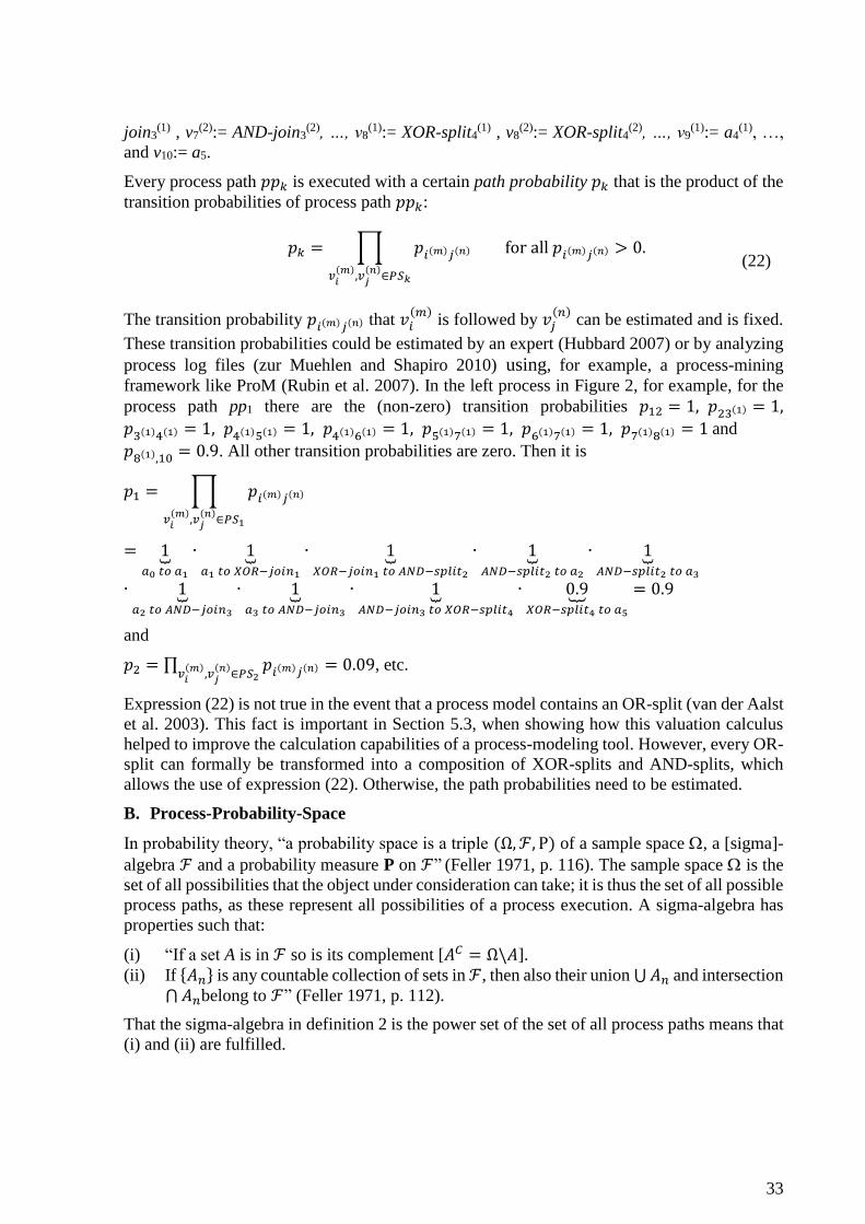
33
join3(1) , v7
(2):= AND-join3(2), …, v8
(1):= XOR-split4(1) , v8
(2):= XOR-split4(2), …, v9
(1):= a4(1), …,
and v10:= a5.
Every process path 𝑝𝑝𝑘 is executed with a certain path probability 𝑝𝑘 that is the product of the
transition probabilities of process path 𝑝𝑝𝑘:
𝑝𝑘 = ∏ 𝑝𝑖(𝑚)𝑗(𝑛)
𝑣𝑖(𝑚)
,𝑣𝑗(𝑛)∈𝑃𝑆𝑘
for all 𝑝𝑖(𝑚)𝑗(𝑛) > 0. (22)
The transition probability 𝑝𝑖(𝑚)𝑗(𝑛) that 𝑣𝑖(𝑚)
is followed by 𝑣𝑗(𝑛)
can be estimated and is fixed.
These transition probabilities could be estimated by an expert (Hubbard 2007) or by analyzing
process log files (zur Muehlen and Shapiro 2010) using, for example, a process-mining
framework like ProM (Rubin et al. 2007). In the left process in Figure 2, for example, for the
process path pp1 there are the (non-zero) transition probabilities 𝑝12 = 1, 𝑝23(1) = 1,
𝑝3(1)4(1) = 1, 𝑝4(1)5(1) = 1, 𝑝4(1)6(1) = 1, 𝑝5(1)7(1) = 1, 𝑝6(1)7(1) = 1, 𝑝7(1)8(1) = 1 and
𝑝8(1),10 = 0.9. All other transition probabilities are zero. Then it is
𝑝1 = ∏ 𝑝𝑖(𝑚)𝑗(𝑛)
𝑣𝑖(𝑚)
,𝑣𝑗(𝑛)∈𝑃𝑆1
= 1⏟𝑎0 𝑡𝑜 𝑎1
∙ 1⏟𝑎1 𝑡𝑜 𝑋𝑂𝑅−𝑗𝑜𝑖𝑛1
∙ 1⏟𝑋𝑂𝑅−𝑗𝑜𝑖𝑛1 𝑡𝑜 𝐴𝑁𝐷−𝑠𝑝𝑙𝑖𝑡2
∙ 1⏟𝐴𝑁𝐷−𝑠𝑝𝑙𝑖𝑡2 𝑡𝑜 𝑎2
∙ 1⏟𝐴𝑁𝐷−𝑠𝑝𝑙𝑖𝑡2 𝑡𝑜 𝑎3
∙ 1⏟𝑎2 𝑡𝑜 𝐴𝑁𝐷−𝑗𝑜𝑖𝑛3
∙ 1⏟𝑎3 𝑡𝑜 𝐴𝑁𝐷−𝑗𝑜𝑖𝑛3
∙ 1⏟𝐴𝑁𝐷−𝑗𝑜𝑖𝑛3 𝑡𝑜 𝑋𝑂𝑅−𝑠𝑝𝑙𝑖𝑡4
∙ 0.9⏟𝑋𝑂𝑅−𝑠𝑝𝑙𝑖𝑡4 𝑡𝑜 𝑎5
= 0.9
and
𝑝2 = ∏ 𝑝𝑖(𝑚)𝑗(𝑛)𝑣𝑖(𝑚)
,𝑣𝑗(𝑛)∈𝑃𝑆2
= 0.09, etc.
Expression (22) is not true in the event that a process model contains an OR-split (van der Aalst
et al. 2003). This fact is important in Section 5.3, when showing how this valuation calculus
helped to improve the calculation capabilities of a process-modeling tool. However, every OR-
split can formally be transformed into a composition of XOR-splits and AND-splits, which
allows the use of expression (22). Otherwise, the path probabilities need to be estimated.
B. Process-Probability-Space
In probability theory, “a probability space is a triple (Ω, ℱ, P) of a sample space , a [sigma]-
algebra ℱ and a probability measure P on ℱ” (Feller 1971, p. 116). The sample space is the
set of all possibilities that the object under consideration can take; it is thus the set of all possible
process paths, as these represent all possibilities of a process execution. A sigma-algebra has
properties such that:
(i) “If a set A is in ℱ so is its complement [𝐴𝐶 = Ω\𝐴].
(ii) If {𝐴𝑛} is any countable collection of sets in ℱ, then also their union ⋃𝐴𝑛 and intersection
⋂𝐴𝑛belong to ℱ” (Feller 1971, p. 112).
That the sigma-algebra in definition 2 is the power set of the set of all process paths means that
(i) and (ii) are fulfilled.

34
“A probability measure P on a [sigma]-algebra ℱ of sets in is a function assigning a value
P{A} 0 to each set A in ℱ such that P{} = 1 and that for every countable collection of non-
overlapping sets An in ℱ [it is] 𝐏{⋃𝐴𝑛} = ∑ 𝐏{𝐴𝑛}𝑛 ” (Feller 1971, p. 115).
All process paths are mutually exclusive, and they represent all possibilities how a process can
be executed. Every process path 𝑝𝑝𝑘 is executed with a certain path probability 𝑝𝑘 > 0. Given
that there is exactly one process path taken if a process is executed and that they are mutual
exclusive, the probabilities 𝑝𝑘 sum up to 1, fulfilling P{} = 1. The property 𝐏{⋃𝐴𝑛} =∑ 𝐏{𝐴𝑛}𝑛 also holds for every countable collection of non-overlapping sets An in ℱ since ℱ is
the power set of .
C. Expected Value of the Process Cash Flow
Let the probability that an action 𝑎𝑑 ∈ 𝐴𝑆, with 𝐴𝑆 ≔ ⋃ 𝐴𝑆𝑘|Ω|𝑘=1 , is executed when executing
a process be
𝑃𝑟(𝑎𝑑): = 𝐏𝑃{𝑃𝑃𝑎𝑑} = ∑𝑝𝑘 ∙ 𝕀𝐴𝑆𝑘(𝑎𝑑)
|Ω|
𝑘=1
with the indicator function
𝕀𝐴𝑆𝑘(𝑎𝑑) = {1, 𝑎𝑑 ∈ 𝐴𝑆𝑘0, 𝑎𝑑 ∉ 𝐴𝑆𝑘
and the set 𝑃𝑃𝑎𝑑 of process paths in which the action 𝑎𝑑 is
𝑃𝑃𝑎𝑑 = {𝑝𝑝𝑘 ∈ Ω|𝑎𝑑 ∈ 𝐴𝑆𝑘}.
Then it is:
𝐸[𝐶𝐹𝑃] = ∑𝐸[𝐶𝐹𝑃|𝑃𝐼 = 𝑘] ∙ 𝑃𝑟𝑜𝑏(𝑃𝐼 = 𝑘)
|Ω|
𝑘=1
=∑𝐸[𝐶𝐹𝑝𝑝𝑘] ∙ 𝑝𝑘
|Ω|
𝑘=1
=∑(𝑝𝑘 ∙ 𝐸 [ ∑ 𝐶𝐹𝑎𝑑𝑎𝑑∈𝐴𝑆𝑘
+∑𝐶𝐹𝑝𝑎𝑠
𝑆
𝑠=1
])
|Ω|
𝑘=1
=∑(𝑝𝑘 ∙ ( ∑ 𝐸[𝐶𝐹𝑎𝑑]
𝑎𝑑∈𝐴𝑆𝑘
+∑𝐸[𝐶𝐹𝑝𝑎𝑠]
𝑆
𝑠=1
))
|Ω|
𝑘=1
=∑( ∑ 𝑝𝑘 ∙ 𝐸[𝐶𝐹𝑎𝑑]
𝑎𝑑∈𝐴𝑆𝑘
)
|Ω|
𝑘=1
+∑(𝑝𝑘 ∙∑𝐸[𝐶𝐹𝑝𝑎𝑠]
𝑆
𝑠=1
)
|Ω|
𝑘=1
=∑( ∑ 𝕀𝐴𝑆𝑘(𝑎𝑑) ∙ 𝑝𝑘 ∙ 𝐸[𝐶𝐹𝑎𝑑]
𝑎𝑑∈𝐴𝑆𝑘
)
|Ω|
𝑘=1
+∑𝐸[𝐶𝐹𝑝𝑎𝑠]
𝑆
𝑠=1
∙ ∑𝑝𝑘
|Ω|
𝑘=1⏟ =1
=∑( ∑ 𝕀𝐴𝑆𝑘(𝑎𝑑) ∙ 𝑝𝑘 ∙ 𝐸[𝐶𝐹𝑎𝑑]
𝑎𝑑∈𝐴𝑆
)
|Ω|
𝑘=1
+∑𝐸[𝐶𝐹𝑝𝑎𝑠]
𝑆
𝑠=1
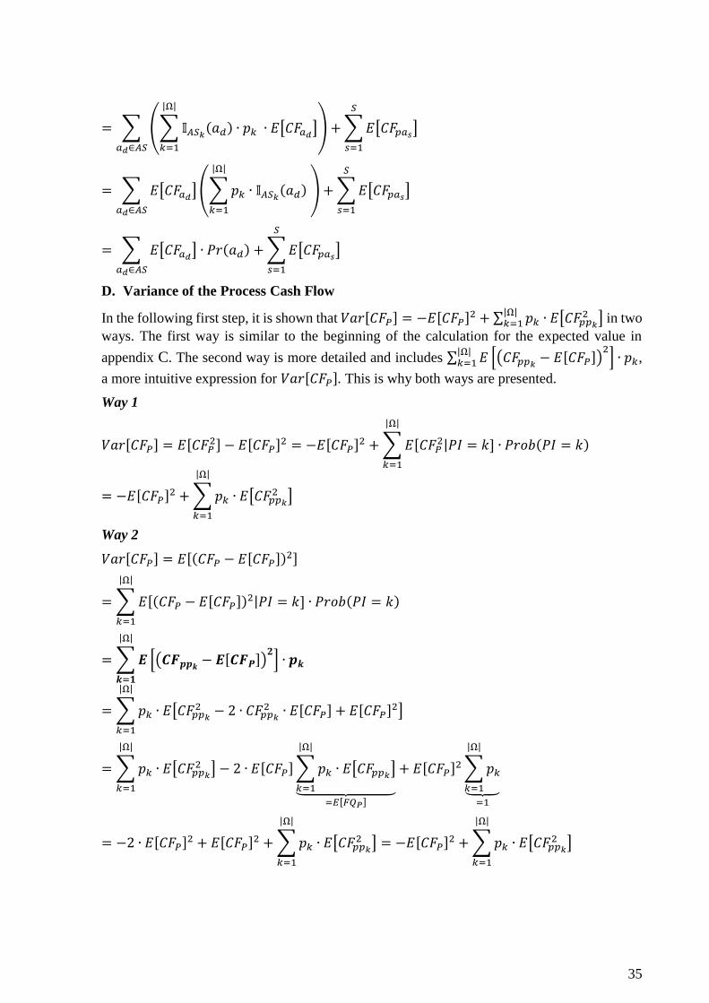
35
= ∑ (∑𝕀𝐴𝑆𝑘(𝑎𝑑) ∙ 𝑝𝑘 ∙ 𝐸[𝐶𝐹𝑎𝑑]
|Ω|
𝑘=1
)
𝑎𝑑∈𝐴𝑆
+∑𝐸[𝐶𝐹𝑝𝑎𝑠]
𝑆
𝑠=1
= ∑ 𝐸[𝐶𝐹𝑎𝑑] (∑𝑝𝑘 ∙ 𝕀𝐴𝑆𝑘(𝑎𝑑)
|Ω|
𝑘=1
)
𝑎𝑑∈𝐴𝑆
+∑𝐸[𝐶𝐹𝑝𝑎𝑠]
𝑆
𝑠=1
= ∑ 𝐸[𝐶𝐹𝑎𝑑] ∙ 𝑃𝑟(𝑎𝑑)
𝑎𝑑∈𝐴𝑆
+∑𝐸[𝐶𝐹𝑝𝑎𝑠]
𝑆
𝑠=1
D. Variance of the Process Cash Flow
In the following first step, it is shown that 𝑉𝑎𝑟[𝐶𝐹𝑃] = −𝐸[𝐶𝐹𝑃]2 + ∑ 𝑝𝑘 ∙ 𝐸[𝐶𝐹𝑝𝑝𝑘
2 ]|Ω|𝑘=1 in two
ways. The first way is similar to the beginning of the calculation for the expected value in
appendix C. The second way is more detailed and includes ∑ 𝐸 [(𝐶𝐹𝑝𝑝𝑘 − 𝐸[𝐶𝐹𝑃])2] ∙ 𝑝𝑘
|Ω|𝑘=1 ,
a more intuitive expression for 𝑉𝑎𝑟[𝐶𝐹𝑃]. This is why both ways are presented.
Way 1
𝑉𝑎𝑟[𝐶𝐹𝑃] = 𝐸[𝐶𝐹𝑃2] − 𝐸[𝐶𝐹𝑃]
2 = −𝐸[𝐶𝐹𝑃]2 +∑𝐸[𝐶𝐹𝑃
2|𝑃𝐼 = 𝑘] ∙ 𝑃𝑟𝑜𝑏(𝑃𝐼 = 𝑘)
|Ω|
𝑘=1
= −𝐸[𝐶𝐹𝑃]2 +∑𝑝𝑘 ∙ 𝐸[𝐶𝐹𝑝𝑝𝑘
2 ]
|Ω|
𝑘=1
Way 2
𝑉𝑎𝑟[𝐶𝐹𝑃] = 𝐸[(𝐶𝐹𝑃 − 𝐸[𝐶𝐹𝑃])2]
=∑𝐸[(𝐶𝐹𝑃 − 𝐸[𝐶𝐹𝑃])2|𝑃𝐼 = 𝑘] ∙ 𝑃𝑟𝑜𝑏(𝑃𝐼 = 𝑘)
|Ω|
𝑘=1
=∑𝑬[(𝑪𝑭𝒑𝒑𝒌 − 𝑬[𝑪𝑭𝑷])𝟐] ∙ 𝒑𝒌
|Ω|
𝒌=𝟏
=∑𝑝𝑘 ∙ 𝐸[𝐶𝐹𝑝𝑝𝑘2 − 2 ∙ 𝐶𝐹𝑝𝑝𝑘
2 ∙ 𝐸[𝐶𝐹𝑃] + 𝐸[𝐶𝐹𝑃]2]
|Ω|
𝑘=1
=∑𝑝𝑘 ∙ 𝐸[𝐶𝐹𝑝𝑝𝑘2 ]
|Ω|
𝑘=1
− 2 ∙ 𝐸[𝐶𝐹𝑃]∑𝑝𝑘 ∙ 𝐸[𝐶𝐹𝑝𝑝𝑘]
|Ω|
𝑘=1⏟ =𝐸[𝐹𝑄𝑃]
+ 𝐸[𝐶𝐹𝑃]2∑𝑝𝑘
|Ω|
𝑘=1⏟ =1
= −2 ∙ 𝐸[𝐶𝐹𝑃]2 + 𝐸[𝐶𝐹𝑃]
2 +∑𝑝𝑘 ∙ 𝐸[𝐶𝐹𝑝𝑝𝑘2 ]
|Ω|
𝑘=1
= −𝐸[𝐶𝐹𝑃]2 +∑𝑝𝑘 ∙ 𝐸[𝐶𝐹𝑝𝑝𝑘
2 ]
|Ω|
𝑘=1

36
In the following second step, it is shown how 𝑉𝑎𝑟[𝐶𝐹𝑃] can be calculated only by using the
expected values and variances of the cash flows of the actions of a process.
Let the probability that both actions 𝑎𝑑 ∈ 𝐴𝑆 and 𝑎𝑗 ∈ 𝐴𝑆, with 𝐴𝑆 ≔ ⋃ 𝐴𝑆𝑘|Ω|𝑘=1 , are executed
when executing a process be
𝑃𝑟(𝑎𝑑, 𝑎𝑗): = 𝐏𝑃 {𝑃𝑃𝑎𝑑,𝑎𝑗} = ∑𝑝𝑘 ∙ 𝕀𝐴𝑆𝑘(𝑎𝑑) ∙ 𝕀𝐴𝑆𝑘(𝑎𝑗)
|Ω|
𝑘=1
with the set 𝑃𝑃𝑎𝑑,𝑎𝑗 of process paths, which contains the action 𝑎𝑑 as well as the action 𝑎𝑗:
𝑃𝑃𝑎𝑑,𝑎𝑗 = {𝑝𝑝𝑘 ∈ Ω|𝑎𝑑 ∈ 𝐴𝑆𝑘, 𝑎𝑗 ∈ 𝐴𝑆𝑘}.
Then it is:
𝑉𝑎𝑟[𝐶𝐹𝑃] =⏞𝑓𝑖𝑟𝑠𝑡 𝑠𝑡𝑒𝑝
− 𝐸[𝐶𝐹𝑃]2 +∑𝑝𝑘 ∙ 𝐸[𝐶𝐹𝑝𝑝𝑘
2 ]
|Ω|
𝑘=1
= −𝐸[𝐶𝐹𝑃]2 +∑𝑝𝑘 ∙ 𝐸 [( ∑ 𝐶𝐹𝑎𝑑
𝑎𝑑∈𝐴𝑆𝑘
+∑𝐶𝐹𝑝𝑎𝑠
𝑆
𝑠=1
)
2
]
|Ω|
𝑘=1
= −𝐸[𝐶𝐹𝑃]2 +∑𝑝𝑘 ∙ 𝐸 [( ∑ 𝐶𝐹𝑎𝑑 ∙ 𝕀𝐴𝑆𝑘(𝑎𝑑)
𝑎𝑑∈𝐴𝑆
+∑𝐶𝐹𝑝𝑎𝑠
𝑆
𝑠=1
)
2
]
|Ω|
𝑘=1
= −𝐸[𝐶𝐹𝑃]2
+∑𝑝𝑘
|Ω|
𝑘=1
∙ 𝐸 [( ∑ 𝐶𝐹𝑎𝑑 ∙ 𝕀𝐴𝑆𝑘(𝑎𝑑)
𝑎𝑑∈𝐴𝑆
)
2
+ 2( ∑ 𝐶𝐹𝑎𝑑 ∙ 𝕀𝐴𝑆𝑘(𝑎𝑑)
𝑎𝑑∈𝐴𝑆
)(∑𝐶𝐹𝑝𝑎𝑠
𝑆
𝑠=1
) + (∑𝐶𝐹𝑝𝑎𝑠
𝑆
𝑠=1
)
2
]
= −𝐸[𝐶𝐹𝑃]2
+∑𝑝𝑘
|Ω|
𝑘=1
∙ 𝐸 [ ∑ 𝐶𝐹𝑎𝑑2 ∙ 𝕀𝐴𝑆𝑘(𝑎𝑑)
𝑎𝑑∈𝐴𝑆
+ ∑ 𝐶𝐹𝑎𝑑 ∙ 𝐶𝐹𝑎𝑗 ∙ 𝕀𝐴𝑆𝑘(𝑎𝑑) ∙ 𝕀𝐴𝑆𝑘(𝑎𝑗)
𝑎𝑑,𝑎𝑗∈𝐴𝑆,𝑎𝑑≠𝑎𝑗
+ 2 ∑ ∑𝐶𝐹𝑎𝑑 ∙ 𝕀𝐴𝑆𝑘(𝑎𝑑) ∙ 𝐶𝐹𝑝𝑎𝑠
𝑆
𝑠=1𝑎𝑑∈𝐴𝑆
+∑𝐶𝐹𝑝𝑎𝑠2
𝑆
𝑠=1
+ 2∑ ∑ 𝐶𝐹𝑝𝑎𝑠 ∙ 𝐶𝐹𝑝𝑎𝑗
𝑆
𝑗=𝑠+1
𝑆−1
𝑠=1
]

37
= −𝐸[𝐶𝐹𝑃]2
+∑𝑝𝑘 ( ∑ 𝐸[𝐶𝐹𝑎𝑑2 ] ∙ 𝕀𝐴𝑆𝑘(𝑎𝑑)
𝑎𝑑∈𝐴𝑆
+∑𝐸[𝐶𝐹𝑝𝑎𝑠2 ]
𝑆
𝑠=1
|Ω|
𝑘=1
+ ∑ 𝐸 [𝐶𝐹𝑎𝑑 ∙ 𝐶𝐹𝑎𝑗] ∙ 𝕀𝐴𝑆𝑘(𝑎𝑑) ∙ 𝕀𝐴𝑆𝑘(𝑎𝑗)
𝑎𝑑,𝑎𝑗∈𝐴𝑆,𝑎𝑑≠𝑎𝑗
+ 2 ∑ ∑𝐸[𝐶𝐹𝑎𝑑 ∙ 𝐶𝐹𝑝𝑎𝑠] ∙ 𝕀𝐴𝑆𝑘(𝑎𝑑)
𝑆
𝑠=1𝑎𝑑∈𝐴𝑆
+ 2∑ ∑ 𝐸 [𝐶𝐹𝑝𝑎𝑠 ∙ 𝐶𝐹𝑝𝑎𝑗]
𝑆
𝑗=𝑠+1
𝑆−1
𝑠=1
)
= −𝐸[𝐶𝐹𝑃]2 + ∑ 𝐸[𝐶𝐹𝑎𝑑
2 ] ∙ (∑𝑝𝑘 ∙ 𝕀𝐴𝑆𝑘(𝑎𝑑)
|Ω|
𝑘=1
)
𝑎𝑑∈𝐴𝑆
+∑𝐸[𝐶𝐹𝑝𝑎𝑠2 ]
𝑆
𝑠=1
∙ ∑𝑝𝑘
|Ω|
𝑘=1⏟ =1
+ ∑ 𝐸 [𝐶𝐹𝑎𝑑 ∙ 𝐶𝐹𝑎𝑗] ∙ (∑𝑝𝑘 ∙ 𝕀𝐴𝑆𝑘(𝑎𝑑) ∙ 𝕀𝐴𝑆𝑘(𝑎𝑗)
|Ω|
𝑘=1
)
𝑎𝑑,𝑎𝑗∈𝐴𝑆,𝑎𝑑≠𝑎𝑗
+ 2 ∑ ∑𝐸[𝐶𝐹𝑎𝑑 ∙ 𝐶𝐹𝑝𝑎𝑠] ∙ (∑𝑝𝑘 ∙ 𝕀𝐴𝑆𝑘(𝑎𝑑)
|Ω|
𝑘=1
)
𝑆
𝑠=1𝑎𝑑∈𝐴𝑆
+ 2∑ ∑ 𝐸 [𝐶𝐹𝑝𝑎𝑠 ∙ 𝐶𝐹𝑝𝑎𝑗]
𝑆
𝑗=𝑠+1
𝑆−1
𝑠=1
∙ ∑𝑝𝑘
|Ω|
𝑘=1⏟ =1
= −𝐸[𝐶𝐹𝑃]2 + ∑ 𝐸[𝐶𝐹𝑎𝑑
2 ] ∙ 𝑃𝑟(𝑎𝑑)
𝑎𝑑∈𝐴𝑆
+∑𝐸[𝐶𝐹𝑝𝑎𝑠2 ]
𝑆
𝑠=1
+ ∑ 𝐸 [𝐶𝐹𝑎𝑑 ∙ 𝐶𝐹𝑎𝑗] ∙ 𝑃𝑟(𝑎𝑑, 𝑎𝑗)
𝑎𝑑,𝑎𝑗∈𝐴𝑆,𝑎𝑑≠𝑎𝑗
+ 2 ∑ ∑𝐸[𝐶𝐹𝑎𝑑 ∙ 𝐶𝐹𝑝𝑎𝑠] ∙ 𝑃𝑟(𝑎𝑑)
𝑆
𝑠=1𝑎𝑑∈𝐴𝑆
+ 2∑ ∑ 𝐸 [𝐶𝐹𝑝𝑎𝑠 ∙ 𝐶𝐹𝑝𝑎𝑗]
𝑆
𝑗=𝑠+1
𝑆−1
𝑠=1
= −𝐸[𝐶𝐹𝑃]2 + ∑ (𝑉𝑎𝑟[𝐶𝐹𝑎𝑑] + 𝐸[𝐶𝐹𝑎𝑑]
2) ∙ 𝑃𝑟(𝑎𝑑)
𝑎𝑑∈𝐴𝑆
+∑(𝑉𝑎𝑟[𝐶𝐹𝑝𝑎𝑠] + 𝐸[𝐶𝐹𝑝𝑎𝑠]2)
𝑆
𝑠=1
+ ∑ (𝐶𝑜𝑣 [𝐶𝐹𝑎𝑑 , 𝐶𝐹𝑎𝑗] + 𝐸[𝐶𝐹𝑎𝑑]𝐸 [𝐶𝐹𝑎𝑗]) ∙ 𝑃𝑟(𝑎𝑑, 𝑎𝑗)
𝑎𝑑,𝑎𝑗∈𝐴𝑆,𝑎𝑑≠𝑎𝑗
+ 2 ∑ ∑(𝐶𝑜𝑣[𝐶𝐹𝑎𝑑 , 𝐶𝐹𝑝𝑎𝑠] + 𝐸[𝐶𝐹𝑎𝑑]𝐸[𝐶𝐹𝑝𝑎𝑠]) ∙ 𝑃𝑟(𝑎𝑑)
𝑆
𝑠=1𝑎𝑑∈𝐴𝑆
+ 2∑ ∑ (𝐶𝑜𝑣 [𝐶𝐹𝑝𝑎𝑠 , 𝐶𝐹𝑝𝑎𝑗] + 𝐸[𝐶𝐹𝑝𝑎𝑠]𝐸 [𝐶𝐹𝑝𝑎𝑗])
𝑆
𝑗=𝑠+1
𝑆−1
𝑠=1

38
= −𝐸[𝐶𝐹𝑃]2 + ∑ (𝑉𝑎𝑟[𝐶𝐹𝑎𝑑] + 𝐸[𝐶𝐹𝑎𝑑]
2) ∙ 𝑃𝑟(𝑎𝑑)
𝑎𝑑∈𝐴𝑆
+∑(𝑉𝑎𝑟[𝐶𝐹𝑝𝑎𝑠] + 𝐸[𝐶𝐹𝑝𝑎𝑠]2)
𝑆
𝑠=1
+ ∑ (𝜌𝑎𝑑,𝑎𝑗 ∙ 𝜎𝑎𝑑 ∙ 𝜎𝑎𝑗 + 𝐸[𝐶𝐹𝑎𝑑]𝐸 [𝐶𝐹𝑎𝑗]) ∙ 𝑃𝑟(𝑎𝑑, 𝑎𝑗)
𝑎𝑑,𝑎𝑗∈𝐴𝑆,𝑎𝑑≠𝑎𝑗
+ 2 ∑ ∑(𝜌𝑎𝑑,𝑝𝑎𝑠 ∙ 𝜎𝑎𝑑 ∙ 𝜎𝑝𝑎𝑠 + 𝐸[𝐶𝐹𝑎𝑑]𝐸[𝐶𝐹𝑝𝑎𝑠]) ∙ 𝑃𝑟(𝑎𝑑)
𝑆
𝑠=1𝑎𝑑∈𝐴𝑆
+ 2∑ ∑ (𝜌𝑝𝑎𝑠,𝑝𝑎𝑗 ∙ 𝜎𝑝𝑎𝑠 ∙ 𝜎𝑝𝑎𝑗 + 𝐸[𝐶𝐹𝑝𝑎𝑠]𝐸 [𝐶𝐹𝑝𝑎𝑗])
𝑆
𝑗=𝑠+1
𝑆−1
𝑠=1
E. Probability of Each Action in Process PR
In order to determine the expected value of 𝐶𝐹𝑃𝑅 we first need to determine the probability of
each action. This is:
𝑃𝑟(𝑎1) = 0.9 + 0.09 + 0.009 +⋯ = 0.9 ∙∑0.1𝑖∞
𝑖=0
= 1,
𝑃𝑟(𝑎2(1)) = 0.9 + 0.09 + 0.009 +⋯ = 0.9 ∙∑0.1𝑖
∞
𝑖=0
= 1,
𝑃𝑟(𝑎2(2)) = 0.09 + 0.009 + 0.0009 +⋯ = 0.09 ∙∑0.1𝑖
∞
𝑖=0
= 0.1,
…,
𝑃𝑟(𝑎3(1)) = 0.9 + 0.09 + 0.009 +⋯ = 0.9 ∙∑0.1𝑖
∞
𝑖=0
= 1,
𝑃𝑟(𝑎3(2)) = 0.09 + 0.009 + 0.0009 +⋯ = 0.09 ∙∑0.1𝑖
∞
𝑖=0
= 0.1,
…,
𝑃𝑟(𝑎4(1)) = 0.09 + 0.009 + 0.0009 +⋯ = 0.09 ∙∑0.1𝑖
∞
𝑖=0
= 0.1,
… .
Thus, it is for example
∑𝑃𝑟(𝑎2(𝑖))
∞
𝑖=1
= ∑0.1𝑖∞
𝑖=0
=1
1 − 0.1=10
9,
which is multiplied with 𝐸[𝐶𝐹𝑎2] since it is 𝐸 [𝐶𝐹𝑎2(𝑖)] = 𝐸[𝐶𝐹𝑎2] for all 𝑖 ∈ ℕ.
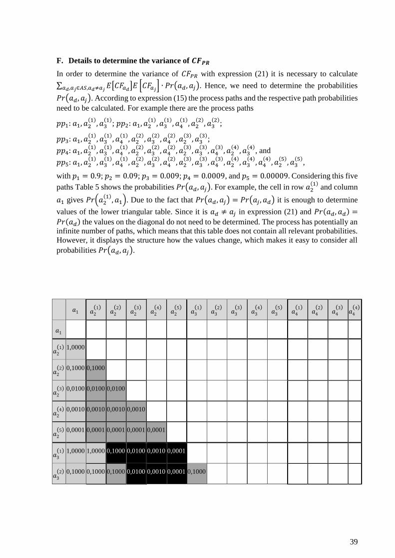
39
F. Details to determine the variance of 𝑪𝑭𝑷𝑹
In order to determine the variance of 𝐶𝐹𝑃𝑅 with expression (21) it is necessary to calculate
∑ 𝐸[𝐶𝐹𝑎𝑑]𝐸 [𝐶𝐹𝑎𝑗] ∙ 𝑃𝑟(𝑎𝑑, 𝑎𝑗)𝑎𝑑,𝑎𝑗∈𝐴𝑆,𝑎𝑑≠𝑎𝑗. Hence, we need to determine the probabilities
𝑃𝑟(𝑎𝑑, 𝑎𝑗). According to expression (15) the process paths and the respective path probabilities
need to be calculated. For example there are the process paths
𝑝𝑝1: 𝑎1, 𝑎2(1), 𝑎3
(1); 𝑝𝑝2: 𝑎1, 𝑎2
(1), 𝑎3(1), 𝑎4
(1), 𝑎2(2), 𝑎3
(2);
𝑝𝑝3: 𝑎1, 𝑎2(1), 𝑎3
(1), 𝑎4(1), 𝑎2
(2), 𝑎3(2), 𝑎4
(2), 𝑎2(3), 𝑎3
(3);
𝑝𝑝4: 𝑎1, 𝑎2(1), 𝑎3
(1), 𝑎4(1), 𝑎2
(2), 𝑎3(2), 𝑎4
(2), 𝑎2(3), 𝑎3
(3), 𝑎4(3), 𝑎2
(4), 𝑎3(4)
, and
𝑝𝑝5: 𝑎1, 𝑎2(1), 𝑎3(1), 𝑎4(1), 𝑎2(2), 𝑎3(2), 𝑎4(2), 𝑎2(3), 𝑎3(3), 𝑎4(3), 𝑎2(4), 𝑎3(4), 𝑎4(4), 𝑎2(5), 𝑎3(5)
,
with 𝑝1 = 0.9; 𝑝2 = 0.09; 𝑝3 = 0.009; 𝑝4 = 0.0009, and 𝑝5 = 0.00009. Considering this five
paths Table 5 shows the probabilities 𝑃𝑟(𝑎𝑑, 𝑎𝑗). For example, the cell in row 𝑎2(1)
and column
𝑎1 gives 𝑃𝑟(𝑎2(1), 𝑎1). Due to the fact that 𝑃𝑟(𝑎𝑑 , 𝑎𝑗) = 𝑃𝑟(𝑎𝑗 , 𝑎𝑑) it is enough to determine
values of the lower triangular table. Since it is 𝑎𝑑 ≠ 𝑎𝑗 in expression (21) and 𝑃𝑟(𝑎𝑑, 𝑎𝑑) =
𝑃𝑟(𝑎𝑑) the values on the diagonal do not need to be determined. The process has potentially an
infinite number of paths, which means that this table does not contain all relevant probabilities.
However, it displays the structure how the values change, which makes it easy to consider all
probabilities 𝑃𝑟(𝑎𝑑, 𝑎𝑗).
𝑎1 𝑎2(1)
𝑎2(2)
𝑎2(3)
𝑎2(4)
𝑎2(5)
𝑎3(1)
𝑎3(2)
𝑎3(3)
𝑎3(4)
𝑎3(5)
𝑎4(1)
𝑎4(2)
𝑎4(3)
𝑎4(4)
𝑎1
𝑎2(1)
1,0000
𝑎2(2)
0,1000 0,1000
𝑎2(3)
0,0100 0,0100 0,0100
𝑎2(4)
0,0010 0,0010 0,0010 0,0010
𝑎2(5)
0,0001 0,0001 0,0001 0,0001 0,0001
𝑎3(1)
1,0000 1,0000 0,1000 0,0100 0,0010 0,0001
𝑎3(2)
0,1000 0,1000 0,1000 0,0100 0,0010 0,0001 0,1000

40
𝑎3(3)
0,0100 0,0100 0,0100 0,0100 0,0010 0,0001 0,0100 0,0100
𝑎3(4)
0,0010 0,0010 0,0010 0,0010 0,0010 0,0001 0,0010 0,0010 0,0010
𝑎3(5)
0,0001 0,0001 0,0001 0,0001 0,0001 0,0001 0,0001 0,0001 0,0001 0,0001
𝑎4(1)
0,1000 0,1000 0,1000 0,0100 0,0010 0,0001 0,1000 0,1000 0,0100 0,0010 0,0001
𝑎4(2)
0,0100 0,0100 0,0100 0,0100 0,0010 0,0001 0,0100 0,0100 0,0100 0,0010 0,0001 0,0100
𝑎4(3)
0,0010 0,0010 0,0010 0,0010 0,0010 0,0001 0,0010 0,0010 0,0010 0,0010 0,0001 0,0010 0,0010
𝑎4(4)
0,0001 0,0001 0,0001 0,0001 0,0001 0,0001 0,0001 0,0001 0,0001 0,0001 0,0001 0,0001 0,0001 0,0001
Table 5 Probabilities 𝐏𝐫(𝐚𝐝, 𝐚𝐣) in Process PR
In Table 5, the values 𝑃𝑟(𝑎𝑑 , 𝑎𝑗) for the same actions 𝑎𝑑 and 𝑎𝑗 are encircled. For example, the
values in the cells of rows 𝑎3(1)
to 𝑎3(5)
and column 𝑎2(1)
to 𝑎2(5)
contain the values for 𝑃𝑟(𝑎𝑑, 𝑎𝑗)
considering the appearance of the actions 𝑎2 and 𝑎3 in the process paths 𝑝𝑝1 to 𝑝𝑝5. All of
these values have to be considered when calculating 𝐸[𝐶𝐹𝑎𝑑]𝐸 [𝐶𝐹𝑎𝑗] ∙ 𝑃𝑟(𝑎𝑑 , 𝑎𝑗) in expression
(21) for the actions 𝑎2 and 𝑎3. The different colors show areas with the same structure of the
values, to know how to use the formula for a geometric series. With this it is possible to
determine ∑ 𝐸[𝐶𝐹𝑎𝑑]𝐸 [𝐶𝐹𝑎𝑗] ∙ 𝑃𝑟(𝑎𝑑, 𝑎𝑗)𝑎𝑑,𝑎𝑗∈𝐴𝑆,𝑎𝑑≠𝑎𝑗 in expression (21).
Overall it is
∑ 𝐸[𝐶𝐹𝑎𝑑]𝐸 [𝐶𝐹𝑎𝑗] ∙ 𝑃𝑟(𝑎𝑑, 𝑎𝑗)
𝑎𝑑,𝑎𝑗∈𝐴𝑆,𝑎𝑑≠𝑎𝑗
= 2⏟𝑑𝑢𝑒 𝑡𝑜 𝑃𝑟(𝑎𝑑,𝑎𝑗)=𝑃𝑟(𝑎𝑗,𝑎𝑑)
∙
[
∑𝐸 [𝐶𝐹𝑎2(𝑖)] 𝐸[𝐶𝐹𝑎1] ∙ 𝑃𝑟(𝑎2
(𝑖), 𝑎1)
∞
𝑖=1⏟ 𝑔𝑟𝑒𝑦 𝑑𝑎𝑠ℎ𝑒𝑑
+∑∑𝐸 [𝐶𝐹𝑎2(𝑖)] 𝐸 [𝐶𝐹
𝑎2(𝑗)] ∙ 𝑃𝑟 (𝑎2
(𝑖), 𝑎2(𝑗))
𝑖−1
𝑗=1
∞
𝑖=2⏟ 𝑑𝑎𝑟𝑘 𝑔𝑟𝑒𝑦

41
+∑𝐸 [𝐶𝐹𝑎3(𝑖)] 𝐸[𝐶𝐹𝑎1] ∙ 𝑃𝑟(𝑎3
(𝑖), 𝑎1)
∞
𝑖=1⏟ 𝑔𝑟𝑒𝑦 𝑑𝑎𝑠ℎ𝑒𝑑
+∑𝐸 [𝐶𝐹𝑎3(𝑖)] 𝐸 [𝐶𝐹
𝑎2(1)] ∙ 𝑃𝑟(𝑎3
(𝑖), 𝑎2(1))
∞
𝑖=1⏟ 𝑔𝑟𝑒𝑦 𝑑𝑎𝑠ℎ𝑒𝑑
+∑∑𝐸 [𝐶𝐹𝑎3(𝑖)] 𝐸 [𝐶𝐹
𝑎2(𝑗)] ∙ 𝑃𝑟 (𝑎3
(𝑖), 𝑎2(𝑗))
𝑖
𝑗=2
∞
𝑖=2⏟ 𝑑𝑎𝑟𝑘 𝑔𝑟𝑒𝑦
+∑ ∑ 𝐸 [𝐶𝐹𝑎3(𝑖)] 𝐸 [𝐶𝐹
𝑎2(𝑗)] ∙ 𝑃𝑟 (𝑎3
(𝑖), 𝑎2(𝑗))
∞
𝑗=𝑖+1
∞
𝑖=1⏟ 𝑏𝑙𝑎𝑐𝑘
+∑∑𝐸 [𝐶𝐹𝑎3(𝑖)] 𝐸 [𝐶𝐹
𝑎3(𝑗)] ∙ 𝑃𝑟 (𝑎3
(𝑖), 𝑎3(𝑗))
𝑖−1
𝑗=1
∞
𝑖=2⏟ 𝑑𝑎𝑟𝑘 𝑔𝑟𝑒𝑦
+∑𝐸 [𝐶𝐹𝑎4(𝑖)] 𝐸[𝐶𝐹𝑎1] ∙ 𝑃𝑟(𝑎4
(𝑖), 𝑎1)
∞
𝑖=1⏟ 𝑤ℎ𝑖𝑡𝑒
+∑𝐸 [𝐶𝐹𝑎4(𝑖)] 𝐸 [𝐶𝐹
𝑎2(1)] ∙ 𝑃𝑟(𝑎4
(𝑖), 𝑎2(1))
∞
𝑖=1⏟ 𝑤ℎ𝑖𝑡𝑒
+∑𝐸 [𝐶𝐹𝑎4(𝑖)] 𝐸 [𝐶𝐹
𝑎2(2)] ∙ 𝑃𝑟(𝑎4
(𝑖), 𝑎2(2))
∞
𝑖=1⏟ 𝑤ℎ𝑖𝑡𝑒
+∑∑𝐸 [𝐶𝐹𝑎4(𝑖)] 𝐸 [𝐶𝐹
𝑎2(𝑗)] ∙ 𝑃𝑟 (𝑎4
(𝑖), 𝑎2(𝑗))
𝑖+1
𝑗=3
∞
𝑖=2⏟ 𝑚𝑖𝑑𝑖𝑢𝑚 𝑑𝑎𝑟𝑘 𝑔𝑟𝑒𝑦
+∑ ∑ 𝐸 [𝐶𝐹𝑎4(𝑖)] 𝐸 [𝐶𝐹
𝑎2(𝑗)] ∙ 𝑃𝑟 (𝑎4
(𝑖), 𝑎2(𝑗))
∞
𝑗=𝑖+2
∞
𝑖=1⏟ 𝑙𝑖𝑔ℎ𝑡 𝑔𝑟𝑒𝑦
+∑𝐸 [𝐶𝐹𝑎4(𝑖)] 𝐸 [𝐶𝐹
𝑎3(1)] ∙ 𝑃𝑟(𝑎4
(𝑖), 𝑎3(1))
∞
𝑖=1⏟ 𝑤ℎ𝑖𝑡𝑒
+∑𝐸 [𝐶𝐹𝑎4(𝑖)] 𝐸 [𝐶𝐹
𝑎3(2)] ∙ 𝑃𝑟(𝑎4
(𝑖), 𝑎3(2))
∞
𝑖=1⏟ 𝑤ℎ𝑖𝑡𝑒
+∑∑𝐸 [𝐶𝐹𝑎4(𝑖)] 𝐸 [𝐶𝐹
𝑎3(𝑗)] ∙ 𝑃𝑟 (𝑎4
(𝑖), 𝑎3(𝑗))
𝑖+1
𝑗=3
∞
𝑖=2⏟ 𝑚𝑖𝑑𝑖𝑢𝑚 𝑑𝑎𝑟𝑘 𝑔𝑟𝑒𝑦
+∑ ∑ 𝐸 [𝐶𝐹𝑎4(𝑖)] 𝐸 [𝐶𝐹
𝑎3(𝑗)] ∙ 𝑃𝑟 (𝑎4
(𝑖), 𝑎3(𝑗))
∞
𝑗=𝑖+2
∞
𝑖=1⏟ 𝑙𝑖𝑔ℎ𝑡 𝑔𝑟𝑒𝑦
+∑∑𝐸 [𝐶𝐹𝑎4(𝑖)] 𝐸 [𝐶𝐹
𝑎4(𝑗)] ∙ 𝑃𝑟 (𝑎4
(𝑖), 𝑎4(𝑗))
𝑖−1
𝑗=1
∞
𝑖=2⏟ 𝑚𝑖𝑑𝑖𝑢𝑚 𝑑𝑎𝑟𝑘 𝑔𝑟𝑒𝑦 ]
= 2 ∙
[
𝐸[𝐶𝐹𝑎2]𝐸[𝐶𝐹𝑎1]∑𝑃𝑟(𝑎2(𝑖), 𝑎1)
∞
𝑖=1⏟ 𝑔𝑟𝑒𝑦 𝑑𝑎𝑠ℎ𝑒𝑑
+ 𝐸[𝐶𝐹𝑎2]𝐸[𝐶𝐹𝑎2]∑∑𝑃𝑟 (𝑎2(𝑖), 𝑎2
(𝑗))
𝑖−1
𝑗=1
∞
𝑖=2⏟ 𝑑𝑎𝑟𝑘 𝑔𝑟𝑒𝑦

42
+𝐸[𝐶𝐹𝑎3]𝐸[𝐶𝐹𝑎1]∑𝑃𝑟(𝑎3(𝑖), 𝑎1)
∞
𝑖=1⏟ 𝑔𝑟𝑒𝑦 𝑑𝑎𝑠ℎ𝑒𝑑
+ 𝐸[𝐶𝐹𝑎3]𝐸[𝐶𝐹𝑎2]∑𝑃𝑟(𝑎3(𝑖), 𝑎2
(1))
∞
𝑖=1⏟ 𝑔𝑟𝑒𝑦 𝑑𝑎𝑠ℎ𝑒𝑑
+ 𝐸[𝐶𝐹𝑎3]𝐸[𝐶𝐹𝑎2]∑∑𝑃𝑟 (𝑎3(𝑖), 𝑎2
(𝑗))
𝑖
𝑗=2
∞
𝑖=2⏟ 𝑑𝑎𝑟𝑘 𝑔𝑟𝑒𝑦
+ 𝐸[𝐶𝐹𝑎3]𝐸[𝐶𝐹𝑎2]∑ ∑ 𝑃𝑟 (𝑎3(𝑖), 𝑎2
(𝑗))
∞
𝑗=𝑖+1
∞
𝑖=1⏟ 𝑏𝑙𝑎𝑐𝑘
+ 𝐸[𝐶𝐹𝑎3]𝐸[𝐶𝐹𝑎3]∑∑𝑃𝑟 (𝑎3(𝑖), 𝑎3
(𝑗))
𝑖−1
𝑗=1
∞
𝑖=2⏟ 𝑑𝑎𝑟𝑘 𝑔𝑟𝑒𝑦
+𝐸[𝐶𝐹𝑎4]𝐸[𝐶𝐹𝑎1]∑𝑃𝑟(𝑎4(𝑖), 𝑎1)
∞
𝑖=1⏟ 𝑤ℎ𝑖𝑡𝑒
+ 𝐸[𝐶𝐹𝑎4]𝐸[𝐶𝐹𝑎2]∑𝑃𝑟(𝑎4(𝑖), 𝑎2
(1))
∞
𝑖=1⏟ 𝑤ℎ𝑖𝑡𝑒
+ 𝐸[𝐶𝐹𝑎4]𝐸[𝐶𝐹𝑎2]∑𝑃𝑟(𝑎4(𝑖), 𝑎2(2))
∞
𝑖=1⏟ 𝑤ℎ𝑖𝑡𝑒
+ 𝐸[𝐶𝐹𝑎4]𝐸[𝐶𝐹𝑎2]∑∑𝑃𝑟 (𝑎4(𝑖), 𝑎2(𝑗))
𝑖+1
𝑗=3
∞
𝑖=2⏟ 𝑚𝑖𝑑𝑖𝑢𝑚 𝑑𝑎𝑟𝑘 𝑔𝑟𝑒𝑦
+ 𝐸[𝐶𝐹𝑎4]𝐸[𝐶𝐹𝑎2]∑ ∑ 𝑃𝑟 (𝑎4(𝑖), 𝑎2
(𝑗))
∞
𝑗=𝑖+2
∞
𝑖=1⏟ 𝑙𝑖𝑔ℎ𝑡 𝑔𝑟𝑒𝑦
+ 𝐸[𝐶𝐹𝑎4]𝐸[𝐶𝐹𝑎3]∑𝑃𝑟(𝑎4(𝑖), 𝑎3
(1))
∞
𝑖=1⏟ 𝑤ℎ𝑖𝑡𝑒
+ 𝐸[𝐶𝐹𝑎4]𝐸[𝐶𝐹𝑎3]∑𝑃𝑟(𝑎4(𝑖), 𝑎3
(2))
∞
𝑖=1⏟ 𝑤ℎ𝑖𝑡𝑒
+ 𝐸[𝐶𝐹𝑎4]𝐸[𝐶𝐹𝑎3]∑∑𝑃𝑟 (𝑎4(𝑖), 𝑎3
(𝑗))
𝑖+1
𝑗=3
∞
𝑖=2⏟ 𝑚𝑖𝑑𝑖𝑢𝑚 𝑑𝑎𝑟𝑘 𝑔𝑟𝑒𝑦
+ 𝐸[𝐶𝐹𝑎4]𝐸[𝐶𝐹𝑎3]∑ ∑ 𝑃𝑟 (𝑎4(𝑖), 𝑎3
(𝑗))
∞
𝑗=𝑖+2
∞
𝑖=1⏟ 𝑙𝑖𝑔ℎ𝑡 𝑔𝑟𝑒𝑦
+𝐸[𝐶𝐹𝑎4]𝐸[𝐶𝐹𝑎4]∑∑𝑃𝑟 (𝑎4(𝑖), 𝑎4
(𝑗))
𝑖−1
𝑗=1
∞
𝑖=2⏟ 𝑚𝑖𝑑𝑖𝑢𝑚 𝑑𝑎𝑟𝑘 𝑔𝑟𝑒𝑦 ]
= 2 ∙
[
𝐸[𝐶𝐹𝑎2]𝐸[𝐶𝐹𝑎1]∑𝑃𝑟(𝑎2(𝑖), 𝑎1)
∞
𝑖=1⏟ 𝑔𝑟𝑒𝑦 𝑑𝑎𝑠ℎ𝑒𝑑
+ 𝐸[𝐶𝐹𝑎2]𝐸[𝐶𝐹𝑎2]∑∑𝑃𝑟 (𝑎2(𝑖), 𝑎2
(𝑗))
𝑖−1
𝑗=1
∞
𝑖=2⏟ 𝑑𝑎𝑟𝑘 𝑔𝑟𝑒𝑦

43
+𝐸[𝐶𝐹𝑎3]𝐸[𝐶𝐹𝑎1]∑𝑃𝑟(𝑎3(𝑖), 𝑎1)
∞
𝑖=1⏟ 𝑔𝑟𝑒𝑦 𝑑𝑎𝑠ℎ𝑒𝑑
+ 𝐸[𝐶𝐹𝑎3]𝐸[𝐶𝐹𝑎2]
(
∑𝑃𝑟(𝑎3
(𝑖), 𝑎2(1))
∞
𝑖=1⏟ 𝑔𝑟𝑒𝑦 𝑑𝑎𝑠ℎ𝑒𝑑
+∑∑𝑃𝑟 (𝑎3(𝑖), 𝑎2
(𝑗))
𝑖
𝑗=2
∞
𝑖=2⏟ 𝑑𝑎𝑟𝑘 𝑔𝑟𝑒𝑦
+∑ ∑ 𝑃𝑟 (𝑎3(𝑖), 𝑎2
(𝑗))
∞
𝑗=𝑖+1
∞
𝑖=1⏟ 𝑏𝑙𝑎𝑐𝑘 )
+ 𝐸[𝐶𝐹𝑎3]𝐸[𝐶𝐹𝑎3]∑∑𝑃𝑟 (𝑎3(𝑖), 𝑎3
(𝑗))
𝑖−1
𝑗=1
∞
𝑖=2⏟ 𝑑𝑎𝑟𝑘 𝑔𝑟𝑒𝑦
+𝐸[𝐶𝐹𝑎4]𝐸[𝐶𝐹𝑎1]∑𝑃𝑟(𝑎4(𝑖), 𝑎1)
∞
𝑖=1⏟ 𝑤ℎ𝑖𝑡𝑒
+ 𝐸[𝐶𝐹𝑎4]𝐸[𝐶𝐹𝑎2]
(
∑𝑃𝑟(𝑎4
(𝑖), 𝑎2(1))
∞
𝑖=1⏟ 𝑤ℎ𝑖𝑡𝑒
+∑𝑃𝑟(𝑎4(𝑖), 𝑎2
(2))
∞
𝑖=1⏟ 𝑤ℎ𝑖𝑡𝑒
+∑∑𝑃𝑟 (𝑎4(𝑖), 𝑎2
(𝑗))
𝑖+1
𝑗=3
∞
𝑖=2⏟ 𝑚𝑖𝑑𝑖𝑢𝑚 𝑑𝑎𝑟𝑘 𝑔𝑟𝑒𝑦
+∑ ∑ 𝑃𝑟 (𝑎4(𝑖), 𝑎2
(𝑗))
∞
𝑗=𝑖+2
∞
𝑖=1⏟ 𝑙𝑖𝑔ℎ𝑡 𝑔𝑟𝑒𝑦 )
+ 𝐸[𝐶𝐹𝑎4]𝐸[𝐶𝐹𝑎3]
(
∑𝑃𝑟(𝑎4
(𝑖), 𝑎3(1))
∞
𝑖=1⏟ 𝑤ℎ𝑖𝑡𝑒
+∑𝑃𝑟(𝑎4(𝑖), 𝑎3
(2))
∞
𝑖=1⏟ 𝑤ℎ𝑖𝑡𝑒
+∑∑𝑃𝑟 (𝑎4(𝑖), 𝑎3
(𝑗))
𝑖+1
𝑗=3
∞
𝑖=2⏟ 𝑚𝑖𝑑𝑖𝑢𝑚 𝑑𝑎𝑟𝑘 𝑔𝑟𝑒𝑦
+∑ ∑ 𝑃𝑟 (𝑎4(𝑖), 𝑎3
(𝑗))
∞
𝑗=𝑖+2
∞
𝑖=1⏟ 𝑙𝑖𝑔ℎ𝑡 𝑔𝑟𝑒𝑦 )
+𝐸[𝐶𝐹𝑎4]𝐸[𝐶𝐹𝑎4]∑∑𝑃𝑟 (𝑎4
(𝑖), 𝑎4(𝑗))
𝑖−1
𝑗=1
∞
𝑖=2⏟ 𝑚𝑖𝑑𝑖𝑢𝑚 𝑑𝑎𝑟𝑘 𝑔𝑟𝑒𝑦 ]
= 2 ∙ [𝐸[𝐶𝐹𝑎2]𝐸[𝐶𝐹𝑎1] ∙10
9
⏟ 𝑔𝑟𝑒𝑦 𝑑𝑎𝑠ℎ𝑒𝑑
+ 𝐸[𝐶𝐹𝑎2]𝐸[𝐶𝐹𝑎2] ∙1
9∑0.1𝑖
∞
𝑖=0⏟ 109⏟
𝑑𝑎𝑟𝑘 𝑔𝑟𝑒𝑦

44
+𝐸[𝐶𝐹𝑎3]𝐸[𝐶𝐹𝑎1] ∙10
9⏟ 𝑔𝑟𝑒𝑦 𝑑𝑎𝑠ℎ𝑒𝑑
+ 𝐸[𝐶𝐹𝑎3]𝐸[𝐶𝐹𝑎2]
(
10
9⏟𝑔𝑟𝑒𝑦 𝑑𝑎𝑠ℎ𝑒𝑑
+1
9∑0.1𝑖
∞
𝑖=0⏟ 𝑑𝑎𝑟𝑘 𝑔𝑟𝑒𝑦
+1
9∑0.1𝑖
∞
𝑖=0⏟ 𝑏𝑙𝑎𝑐𝑘 )
+ 𝐸[𝐶𝐹𝑎3]𝐸[𝐶𝐹𝑎3] ∙1
9∑0.1𝑖
∞
𝑖=0⏟ 𝑑𝑎𝑟𝑘 𝑔𝑟𝑒𝑦
+𝐸[𝐶𝐹𝑎4]𝐸[𝐶𝐹𝑎1] ∙1
9⏟ 𝑤ℎ𝑖𝑡𝑒
+ 𝐸[𝐶𝐹𝑎4]𝐸[𝐶𝐹𝑎2]
(
1
9⏟𝑤ℎ𝑖𝑡𝑒
+1
9⏟𝑤ℎ𝑖𝑡𝑒
+1
90∑0.1𝑖
∞
𝑖=0⏟ 𝑚𝑖𝑑𝑖𝑢𝑚 𝑑𝑎𝑟𝑘 𝑔𝑟𝑒𝑦
+1
90∑0.1𝑖
∞
𝑖=0⏟ 𝑙𝑖𝑔ℎ𝑡 𝑔𝑟𝑒𝑦 )
+ 𝐸[𝐶𝐹𝑎4]𝐸[𝐶𝐹𝑎3]
(
1
9⏟𝑤ℎ𝑖𝑡𝑒
+1
9⏟𝑤ℎ𝑖𝑡𝑒
+1
90∑0.1𝑖
∞
𝑖=0⏟ 𝑚𝑖𝑑𝑖𝑢𝑚 𝑑𝑎𝑟𝑘 𝑔𝑟𝑒𝑦
+1
90∑0.1𝑖
∞
𝑖=0⏟ 𝑙𝑖𝑔ℎ𝑡 𝑔𝑟𝑒𝑦 )
+𝐸[𝐶𝐹𝑎4]𝐸[𝐶𝐹𝑎4] ∙
1
90∑0.1𝑖
∞
𝑖=0⏟ 𝑚𝑖𝑑𝑖𝑢𝑚 𝑑𝑎𝑟𝑘 𝑔𝑟𝑒𝑦 ]
= 2 ∙ [500 ∙ 1,000 ∙10
9
⏟ 𝑔𝑟𝑒𝑦 𝑑𝑎𝑠ℎ𝑒𝑑
+ 500 ∙ 500 ∙10
81⏟ 𝑑𝑎𝑟𝑘 𝑔𝑟𝑒𝑦
+500 ∙ 1,000 ∙10
9⏟ 𝑔𝑟𝑒𝑦 𝑑𝑎𝑠ℎ𝑒𝑑
+ 500 ∙ 500(10
9⏟𝑔𝑟𝑒𝑦 𝑑𝑎𝑠ℎ𝑒𝑑
+10
81⏟𝑑𝑎𝑟𝑘 𝑔𝑟𝑒𝑦
+10
81⏟𝑏𝑙𝑎𝑐𝑘
)+ 500 ∙ 500 ∙10
81⏟ 𝑑𝑎𝑟𝑘 𝑔𝑟𝑒𝑦
+5,000 ∙ 1,000 ∙1
9⏟ 𝑤ℎ𝑖𝑡𝑒
+ 5,000 ∙ 500(1
9⏟𝑤ℎ𝑖𝑡𝑒
+1
9⏟𝑤ℎ𝑖𝑡𝑒
+1
81⏟𝑚𝑖𝑑𝑖𝑢𝑚 𝑑𝑎𝑟𝑘 𝑔𝑟𝑒𝑦
+1
81⏟𝑙𝑖𝑔ℎ𝑡 𝑔𝑟𝑒𝑦
)+ 5,000
∙ 500(1
9⏟𝑤ℎ𝑖𝑡𝑒
+1
9⏟𝑤ℎ𝑖𝑡𝑒
+1
81⏟𝑚𝑖𝑑𝑖𝑢𝑚 𝑑𝑎𝑟𝑘 𝑔𝑟𝑒𝑦
+1
81⏟𝑙𝑖𝑔ℎ𝑡 𝑔𝑟𝑒𝑦
)+5,000 ∙ 5,000 ∙1
81⏟ 𝑚𝑖𝑑𝑖𝑢𝑚 𝑑𝑎𝑟𝑘 𝑔𝑟𝑒𝑦
]
= 2 ∙ [500 ∙ 1,000 ∙10
9+ 500 ∙ 500 ∙
10
81
+500 ∙ 1,000 ∙10
9+ 500 ∙ 500 ∙
110
81+ 500 ∙ 500 ∙
10
81
+5,000 ∙ 1,000 ∙1
9+ 5,000 ∙ 500 ∙
20
81+ 5,000 ∙ 500 ∙
20
81+5,000 ∙ 5,000 ∙
1
81]

45
References Appendix
Feller W (1971) An Introduction to Probability Theory and Its Applications, Vol. 2. John Wiley
& Sons, Inc., New York, NY, USA
Gibbons A (1985) Algorithmic Graph Theory. Cambridge University Press, Melbourne,
Australia
Hollingsworth DC, WfMC (2003) The WfMC Glossary. In: Fischer L (ed) Workflow
Handbook 2003. Future Strategies Inc., Lighthouse Point, Florida, USA, pp 263-299
Hubbard DW (2007) How to Measure Anything: Finding the Value of Intangibles in Business.
John Wiley & Sons, Inc., New York, NY, USA
Rubin V, Günther CW, van der Aalst WMP, Kindler E, van Dongen BF, Schäfer W (2007)
Process mining framework for software processes. In: Wang Q, Pfahl D, Raffo DM (eds)
Proceedings of the International Conference on Software Process: Software Process Dynamics
and Agility (ICSP), Minneapolis, MN, USA, pp 169-181
van der Aalst WMP, ter Hofstede AH, Kiepuszewski B, Barros AP (2003) Workflow patterns.
Distrib Parallel Dat 14(3):5-51
zur Muehlen M, Shapiro R (2010) Business Process Analytics. In: vom Brocke J, Rosemann M
(eds) Handbook on Business Process Management 2: Strategic Alignment, Governance, People
and Culture. Springer, Berlin, Germany, pp 137-158


![Bonita Open Solution why, what, how? · 2015-11-09 · OMG! It’s Business Process [Eclipse] Modeling in Bonita Open Solution Aurélien Pupier R&D Engineer, Studio Project Leader](https://img.pdfslide.us/doc/110x75/5e994d1a1cf79255062314fd/bonita-open-solution-why-what-how-2015-11-09-omg-itas-business-process-eclipse.jpg)