BRAIN DRAIN IN RURAL AMERICA

Brigitte S. Waldorf

Department of Agricultural Economics, Purdue University West Lafayette, IN 47907, USA Email: bwaldorf@purdue.edu;

Selected Paper prepared for presentation at the American Agricultural Economics Association

Annual Meeting, Portland, Oregon, July 28-30, 2007

© Copyright 2007 by Brigitte Waldorf. All rights reserved. Readers may make verbatim copies of this document for non-commercial purposes by any means, provided that this copyright notice appears on such copies.

1

Abstract: The paper aims at understanding changes in the distribution and accumulation of intellectual capital by analyzing migrants’ educational profiles across a sample of 303 U.S. counties. The results suggest that newcomers are better educated than the resident population, and the education gap is most pronounced for newcomers from other states. The results further suggest that the educational status of newcomers (“in-migrants”) is positively related to the educational status of the resident population (“stayers”), thus implying a further agglomeration of human capital across space. However, for interstate migrants the effect is context-dependent, playing a greater role in urban than in rural settings. Keywords: Human Capital, Migration, Brain Drain,

JEL Classification: J24, R23 1. Introduction Since the 1960s, the United States experienced a remarkable rise in educational attainment levels. However, the education boom did not affect all places equally and many regions have not been successful in accumulating intellectual capital. Selective migration behaviors of the highly-educated play a substantial role in creating these inequalities. This winner-loser situation –commonly referred to as brain gain and brain drain– is epitomized in the simultaneous occurrence of knowledge-based regional economies such as California’s Silicon Valley and the Research Triangle in North Carolina and large pockets of educational deprivation such as in the rural South.

The selective migration of the highly educated population is a serious concern in regions suffering from a persistent brain drain. For example, many Midwestern States have been losing a substantial share of their well-educated residents to other states (Schachter et al. 2003, Franklin 2003, Waldorf 2007, Whisler et al. 2007) and a recent report from the Brookings Institution (Austin and Affolter Caine 2006) identified the underdeveloped human capital base as one of the key challenges for the Great Lake region as it struggles to retain its economic and social viability. The lack of human capital becomes even more pronounced when zooming in to a smaller spatial scale. At the county level, Waldorf (2006a) identified severe disparities in educational attainment across Indiana, with educational attainment profiles in many counties lagging behind by quite a margin, often having a .

This paper aims at understanding changes in the distribution and accumulation of intellectual capital by analyzing migrants’ educational profiles across a sample of U.S. counties. Two sets of questions are addressed. The first set is exploratory in nature, juxtaposing the educational attainment levels of those who did not move, i.e., the stayers, and those who moved into the county, i.e., the newcomers. Specifically, it explores variations in migrants’ educational attainment levels across space, identifying places with the highest shares of highly-educated migrants. Are these places randomly distributed, do they cluster in space, and do the landscapes of educational status differ for stayers and migrants? This set of questions also addresses whether newcomers, on average, are better educated than those already living in an area, and whether the educational gap differ by migrant origin.

The second set of questions addresses an important stock-flow relationship that may contribute to persistent and even intensifying disparities in educational attainment levels across space. Specifically, does educational deprivation of a region’s population (stock) dampen the inflow of the well-educated? Is this effect uniform across space or does it differ between rural and urban areas? The answers will have important consequences for the emergence of “brain-rich” and brain-poor” regions. If indeed a better educated stock attracts a better educated group of migrants, then the results suggest a spatial sorting such that areas with a poorly educated population will face difficulties attracting educated migrants.

2

Consequently, the already uneven spatial distribution of the highly educated population will become increasingly concentrated, creating disparities between brain-rich and brain-poor regions. This poses severe challenges for regions that are already lagging as they are at high risk of being further left behind.

The empirical analysis is carried out using data for a sample of counties from 18 states, stretching from Massachusetts in the East to Nebraska in the West, and from the Canadian border to Tennessee. Data on educational attainment levels of migrants and stayers are taken from the 2005 American Community Survey (ACS), and are linked with 2000 U.S. census data on a host of control variables. A series of descriptive statistics – including a summary measure of educational status – are used to investigate differences in the educational profiles of movers and stayers. Locational variations are discovered through trend surfaces of the share of highly educated migrants, segmented by degree of rurality. Finally, the stock-flow relationships are addressed in a series of regression models that link the educational status of migrants to the educational status of stayers, controlling for the degree of rurality, spatial trends, and the county’s demographic make-up, housing characteristics and industrial structure.

The paper is comprised of four sections. Following this introduction, the second section provides a general background on spatio-temporal changes in educational attainment levels in the United States and the hypotheses to be tested. The third section presents the empirical analysis, and includes subsections on the data, methods used, and the empirical results. The paper ends with a summary, future research directions, and implications for regional economic policies. 2. Background

The highly-educated are the most mobile segment of the U.S. population. They move frequently and do not shy away from long distances (Basker 2002, Kodrzycki 2001). They also have very distinct, amenity-driven locational preferences (Whisler et al. 2007) and, given their high income potential, they are capable of realizing those preferences by relocating to the most desirable places. Clark et al. (2002) observe that for the highly educated workforce “[t]he decision about where to live and enjoy life can play as large or a larger role than the job offer itself in the final location decision” (p. 513). Distinct locational preferences may also be the result of new demographic groups, such as the ‘power couples’ (Costa and Kahn 2000) that have to negotiate joint locational needs.

0

5

10

15

20

25

30

1970 1980 1990 2000 Year

% a

dults

with

at l

east

a

bach

elor

's d

egre

e

non-metro

metro US

Figure 1. Percent Adults (age 25+) with at least a college degree, 1970 to 2005

Figure 1 shows the growth of the highly educated population over time. Whereas in

1970 the percentage of persons age 25 and older with at least a four-year college degree was only 10.7 percent, it increased by 5.5 percentage points to 16.2% in 1980, and by additional four percentage points in each of the two subsequent decades. Today, about one quarter of the

3

adult1 population has earned at least a four-year college degree. This remarkable increase at a high speed is accompanied by a comparable decline in the population at the other end of the educational attainment scale, namely those who did not complete high school. In 1970, nearly half of the adult American population did not have a high school degree. By the year 2000, only one fifth of the population falls into that category.2 Figure 1 also shows that traditionally the college-educated population bas been over-represented in metropolitan areas. Over time, the metro/non-metro gap has been widening, amounting to only to 4.8 percentage points in 1970, but more than doubled to 11.3 percentage points in the year 2000. The unprecedented growth of the highly educated population –coupled with its high migration propensities and its distinct locational preferences– thus has the potential to trigger substantial shifts in overall migration patterns and ultimately in the distribution of the population across the United States. The highly-educated are also the most sought-after segment of the labor force. Post-industrial societies rely strongly on a highly-educated workforce to meet new demands created by the increasing share of managerial and professional jobs.3 Moreover, the literature contents that human capital propels regional economic growth (Mathur 1999, Waldorf 2007) In fact, intellectual power is seen as the driving force for a vibrant business climate, spurring entrepreneurial spirit, and attracting businesses and industries from around the world (see e.g., Cooke 2002, Karlsson et al. 2004, Greunz 2004, Waldorf 2006a, 2007). Henderson and Abraham (2002) refer to knowledge as the “new fuel powering economic growth in the 21st century” (p. 88).

The question thus arises what factors influence the spatial concentration of intellectual capital and, in particular, whether human capital accumulation is a self-propelling process. Large and growing concentrations of the highly educated population are not found in all metropolitan areas but primarily in big metro areas that benefit the most from agglomeration economies. Large urban areas with their abundance of managerial and professional jobs are often the preferred destinations of the highly educated (Costa and Kahn 2000, Florida 2002b, McCann and Sheppard 2002, Ritsilä and Haapanen 2003, Schachter et al. 2003). Moreover, man-made and natural amenities are pivotal in attracting the highly-educated work force (Glaeser et al. 2000, Florida 2002a, 2002b). The literature also suggests that the human capital stock itself may take on the role of a “pull factor” that attracts additional, highly educated migrants and reduces out migration rates. For the college-educated of all ages, Whisler et al. (2007) find that the propensity to leave metropolitan areas are inversely related to human capital growth. Thus, metropolitan areas that –over a prolonged time– cannot build a highly-educated workforce are at risk of falling behind in today’s knowledge economy.

If human capital accumulation is a self-propelling process and the big metro-areas get more than their fair share of intellectual capital, then one also has to ask whether brain drain is a self-propelling process. That is, once set in motion and manifested in an underdeveloped human capital base, will the brain drain continue through increased out-migration and reduced in-migration rates? The empirical analysis presented in the subsequent will address

1 Persons of age 25 or older. 2 It is reasonable to suspect that much of this drop is simply due to age-related mortality differences between the traditionally less educated older population and the younger, more educated population. 3 Between 1990 and 2000, only management and professional occupations have substantially increased their share in the U.S. labor force over the last decade. The share of service occupations increased slightly by less than one percentage point. All other occupation categories saw their shares dwindle (Special Equal Employment Opportunity (EEO) Tabulations (www.census.gov)). .

4

this question, testing the hypotheses (a) that the educational status of in-migrants is positively related to the educational status of the resident population and (b) that this effect is context dependent, decreasing with in more rural settings. 3. Empirical Analysis

The empirical analysis focuses on a region comprised of 18 states4 that stretch from the East Coast to the Prairie states and from the Canadian border to Tennessee. It thus includes highly urbanized parts of the East Coast megalopolis, as well as the very rural places in the Dakotas and Nebraska. Moreover, the study region includes the Midwestern states that offer more mixed settings: rural areas with extensive corn and soybean farming in close proximity to old manufacturing strongholds such as the steel industry in Gary, Indiana and the automobile industry in Detroit, Michigan. The transition to a knowledge-based economy takes on added significance in these states since their competitive advantages – such as low labor costs in rural areas – continue to erode in the face of ever stronger global competition. In light of these new economic realities, failure to accumulate intellectual capital thus threatens the ability to compete (see, e.g., Lichter et al. 1992, Munnich et al. 2002). Table 1. Percent of Population (age 25+) with a Four-year College Degree in Selected States, 1970 to 2000

Above the national average

1970 1980 1990 2000 Below the national average

1970 1980 1990 2000

MA 12.6 20.0 27.2 33.2 NE 9.6 15.5 18.9 23.7 NJ 11.8 18.3 24.9 29.8 PA 8.7 13.6 17.9 22.4 NY 11.9 17.9 23.1 27.4 WI 9.8 14.8 17.7 22.4 MN 11.1 17.4 21.8 27.4 ND 8.4 14.8 18.1 22.0 IL 10.3 16.2 21.0 26.1 MI 9.4 14.3 17.4 21.8 KS 11.4 17.0 21.1 25.8 MO 9.0 13.9 17.8 21.6

SD 8.6 14.0 17.2 21.5 IA 9.1 13.9 16.9 21.2 OH 9.3 13.7 17.0 21.1 TN 7.9 12.6 16.0 19.6 IN 8.3 12.5 15.6 19.4 KY 7.2 11.1 13.6 17.1

US 10.7 16.2 20.3 24.4 Table 1 traces the percentage of the college-educated population in the 18 states from

1970 to 2000. On the left-hand side are the six states that exceed the national percentage. They are topped by the three East Coast states and followed by Minnesota, Illinois and Kansas. With the exception of Illinois, these states have persistently outperformed the nation as a whole and even been able to extend their lead. Illinois exceeded the national percentage of college educated residents starting in 1990 and has by now surpassed Kansas. On the right-hand side of the table are the states with below average share of highly educated residents. Kentucky, Indiana, and Tennessee lag most severely behind the national average. Looking at the extremes, in Massachusetts is the percentage of college-educated resident almost twice as high as in Kentucky.

4 The states included in the analysis are: Illinois, Indiana, Iowa, Kansas, Kentucky, Massachusetts, Michigan, Minnesota, Missouri, Nebraska, New Jersey, New York, North Dakota, Ohio, Pennsylvania, South Dakota, Pennsylvania, and Wisconsin.

5

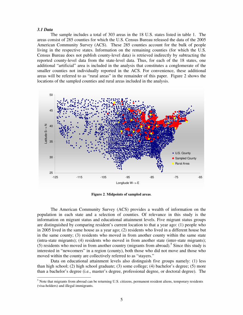
3.1 Data The sample includes a total of 303 areas in the 18 U.S. states listed in table 1. The

areas consist of 285 counties for which the U.S. Census Bureau released the data of the 2005 American Community Survey (ACS). These 285 counties account for the bulk of people living in the respective states. Information on the remaining counties (for which the U.S. Census Bureau does not publish county-level data) is retrieved indirectly by subtracting the reported county-level data from the state-level data. Thus, for each of the 18 states, one additional “artificial” area is included in the analysis that constitutes a conglomerate of the smaller counties not individually reported in the ACS. For convenience, these additional areas will be referred to as “rural areas” in the remainder of this paper. Figure 2 shows the locations of the sampled counties and rural areas included in the analysis.

25

30

35

40

45

50

-125 -115 -105 -95 -85 -75 -65

Longitude W--> E

Latit

ude

S--

> N

U.S. County

Sampled County

Rural Area

Figure 2. Midpoints of sampled areas.

The American Community Survey (ACS) provides a wealth of information on the population in each state and a selection of counties. Of relevance in this study is the information on migrant status and educational attainment levels. Five migrant status groups are distinguished by comparing resident’s current location to that a year ago: (1) people who in 2005 lived in the same house as a year ago; (2) residents who lived in a different house but in the same county; (3) residents who moved in from another county within the same state (intra-state migrants); (4) residents who moved in from another state (inter-state migrants); (5) residents who moved in from another country (migrants from abroad).5 Since this study is interested in “newcomers” in a region (county), both those who did not move and those who moved within the county are collectively referred to as “stayers.”

Data on educational attainment levels also distinguish five groups namely: (1) less than high school; (2) high school graduate; (3) some college; (4) bachelor’s degree; (5) more than a bachelor’s degree (i.e., master’s degree, professional degree, or doctoral degree). The 5 Note that migrants from abroad can be returning U.S. citizens, permanent resident aliens, temporary residents (visa-holders) and illegal immigrants.

6

ACS provides estimates (and margins of error) for the number of people in each category, further disaggregated by migrant status. Table 2. Variable Definition and Summary Statistics across Sampled Counties and Rural Areas

Variable Definition Average Standard Deviation Minimum Maximum

Same house Percent Pop 25+ that lived in the same house a year ago, 2005 87.844 2.611 78.567 93.116

Same County Percent Pop 25+ that lived in a different house but same county a year ago, 2005

7.209 2.001 2.703 13.376

Intra-state Migrants

Percent Pop 25+ that lived in a different county but same state a year ago, 2005

2.681 1.279 0.444 6.744

Inter-state Migrants

Percent Pop 25+ that lived in a different state a year ago, 2005 1.883 1.083 0.334 7.448

Migrants from Abroad

Percent Pop 25+ that lived in a different country a year ago, 2005

0.383 0.376 0.000 2.838

Less than HS Percent Pop 25+ Less than high school graduate, 2005 12.373 4.160 3.955 31.925

HS Percent Pop 25+ High school graduate, 2005 33.248 6.968 13.548 52.166

Some College Percent Pop 25+ with some college or associate's degree, 2005

27.650 4.412 13.922 37.908

Bachelor Percent Pop 25+ with Bachelor's degree, 2005 16.913 5.512 6.649 35.750

Grad/Prof Percent Pop 25+ with graduate or professional degree, 2005 9.815 4.583 3.578 29.763

IRR 2000 Index of Relative Rurality - continuous measure; ranges from 0 (most urban) to 1( most rural).

0.297 0.133 0.038 0.686

Latitude Degrees north of the equator 41.148 2.280 35.096 47.909

Longitude Degrees west (negative) of the Greenwich meridian -83.851 7.298 -103.105 -70.302

%Black Percentage of the population that self-identifies itself as black, 2000

6.749 7.808 0.086 48.380

%foreign born Percent of the population that was born outside the U.S., 2000 5.163 6.125 0.563 46.127

%65+ Percent of the population 65 years old or older, 2000 12.769 2.746 6.195 23.068

% Mobile Percent of housing units classified as mobile housing, 2000

5.481 4.343 0.030 20.505

Housing Cost

Percent of homeowners paying less than 30% of their income on housing-related costs (mortgage, insurance, taxes), 2000

23.149 5.257 13.728 46.323

Mfg Percent of employment in the manufacturing cluster, 2004 6.374 5.225 0.000 33.930

The ACS data are linked with information from the 2000 U.S. census that that relates

to important demographic characteristics including the percentages of elderly (age 65+) residents, black residents, and foreign-born residents. Attributes of the housing market

7

include the percentage of mobile homes and the percentage of home owners paying less than 30% of their income on housing-related costs (i.e., mortgage, insurance, and taxes). This latter variable is taken as a proxy for cost-of-living. The employment share in the manufacturing cluster6 is used to characterize the industry structure. Finally, three spatial variables are included in the analysis. Longitude and latitude of county midpoints provide the necessary information to describe spatial trends across the 18-state region. The index of relative rurality (Waldorf 2006b), which combines information on population size, density, and distance to the closest metropolitan area, is used to distinguish the counties and rural areas by their degree of rurality. The summary statistics for the data are listed in table 2.

3.2 Methods

The locational variation in educational status is assessed by fitting a series of trend surfaces. A trend surface expresses a variable as a –typically polynomial– function of longitude and latitude. The analysis fits trend surfaces to the educational status variable for the entire sample as well as for sample segments stratified by the degree of rurality.

The well-known dissimilarity index (Duncan and Duncan 1955) is used to assess differences in educational status among the groups. The dissimilarity index is defined as:

DI=½*�k |Sk-Mk| ∈[0.100], where Sk is the percentage share of persons with educational attainment k among the stayers and Mk is the percentage share of persons with educational attainment k among movers. The dissimilarity index indicates the percentage of the mover group that would have to belong into a different educational attainment group so as to achieve complete similarity with the stayer group. Thus, a value of zero implies complete similarity, a value of 100 means complete dissimilarity between movers and stayers.

The dissimilarity index only responds to similarities across the educational attainment levels, but dos not address the issue of whether newcomers are, on average, better educated than stayers. Thus, an educational status variable is developed that uses the nation’s educational attainment profile as a benchmark of comparison. For each population group i, (mover or stayer) and each county j, the educational status variable takes on the form:

ESij = HUS – Hij + Cij – CUS, where H is the percentage with at most a high school degree, C is the percentage with at least a four-year college degree, and the subscripts US and ij indicate whether the percentages refer to the nation as a whole or to population group i in county j, respectively. In essence, the educational status indicates the “beneficial” deviation from the nation’s educational profile, expressed in percentage points. The lower bound of the educational status variable is HUS – 100 – CUS (the group consists entirely of persons with a high school degree or less), and the upper bound is HUS + 100 – CUS (everybody has at least a college degree). To capture the stock-flow relationships, I estimated two sets of regression models. The first set uses the percentage of highly educated migrants (at least a college degree) as the dependent variable and the second set uses the educational status variable as the dependent variable. Among the exogenous variables, the percentage of highly educated stayers (or, stayers’educational status) is the key variable. It is expected that it has a positive effect on the dependent variable and thus testing the notion that brain gain and brain drain are self-perpetuating processes.

6 The manufacturing cluster is made up of all manufacturing employment plus the employment of industries that are intricately linked with manufacturing. The data were taken from a recent study on industry clusters (Purdue Center for Regional Development and Indiana Business Research Center 2007). The data are available at http://www.ibrc.indiana.edu/innovation/data.html . A detailed listing of all NAICS codes included in the manufacturing cluster is provided at: http://www.ibrc.indiana.edu/innovation/reports/sections/appendix_I.pdf

8

The models are then enhanced by adding the interaction between the rurality index and stayers’ education. It is hypothesized that the interaction term has a negative parameter, and thus that the self-perpetuating forces decrease with increasing rurality. All models include a set of controls for spatial trends (longitude and latitude), rurality (IRR), attributes describing the population (% elderly, % black, % foreign-born), characteristics of the housing market (% mobile homes, % less than 30%) and industry structure (% manufacturing). Separate models are estimated for each type of newcomer (intra-state, interstate, from abroad). 3.3 The Education Gap between Movers and Stayers

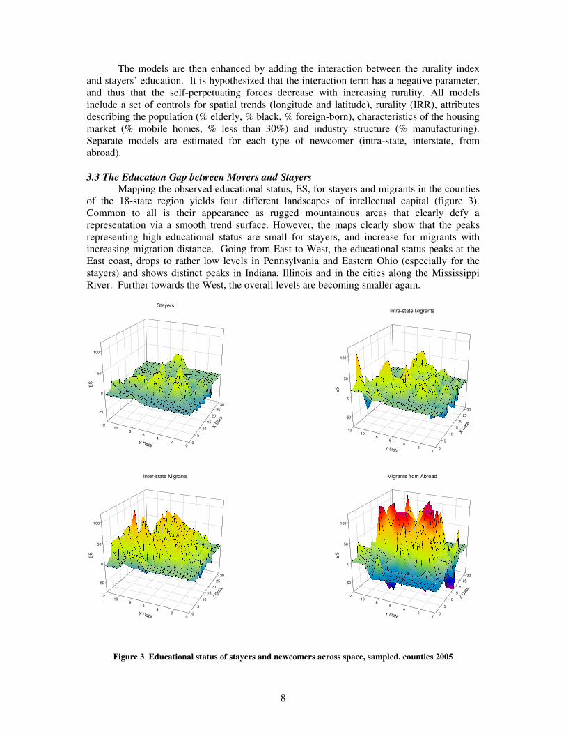
Mapping the observed educational status, ES, for stayers and migrants in the counties of the 18-state region yields four different landscapes of intellectual capital (figure 3). Common to all is their appearance as rugged mountainous areas that clearly defy a representation via a smooth trend surface. However, the maps clearly show that the peaks representing high educational status are small for stayers, and increase for migrants with increasing migration distance. Going from East to West, the educational status peaks at the East coast, drops to rather low levels in Pennsylvania and Eastern Ohio (especially for the stayers) and shows distinct peaks in Indiana, Illinois and in the cities along the Mississippi River. Further towards the West, the overall levels are becoming smaller again.

Figure 3. Educational status of stayers and newcomers across space, sampled. counties 2005

-50

0

50

100

0

5

10

15

20

2530

02

46

810

12

ES

X Dat

a

Y Data

Intra-state Migrants

-50

0

50

100

0

5

10

15

20

2530

02

46

810

12

ES

X Dat

a

Y Data

Inter-state Migrants

-50

0

50

100

0

5

10

15

20

2530

02

46

810

12

ES

X Dat

a

Y Data

Migrants from Abroad

-50

0

50

100

0

5

10

15

20

2530

02

46

810

12

ES

X Dat

a

Y Data

Stayers

9

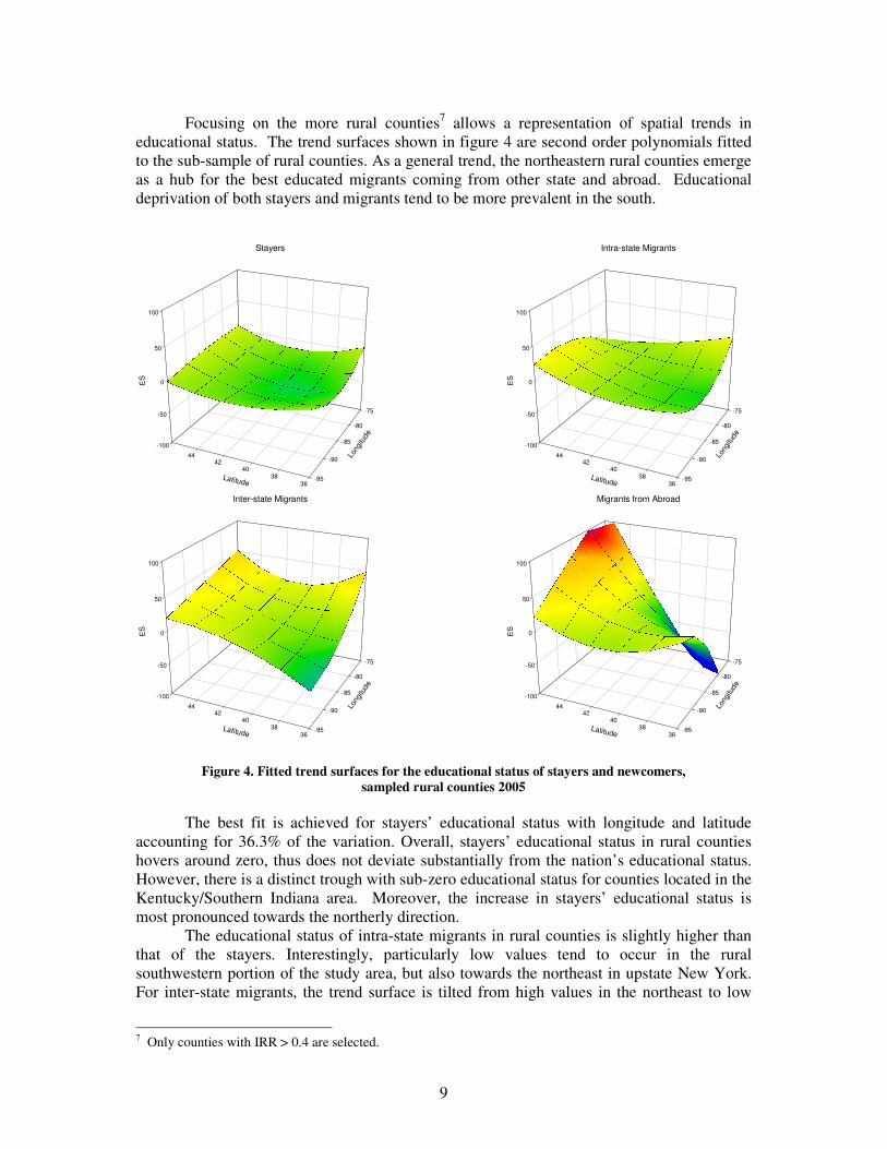
Focusing on the more rural counties7 allows a representation of spatial trends in

educational status. The trend surfaces shown in figure 4 are second order polynomials fitted to the sub-sample of rural counties. As a general trend, the northeastern rural counties emerge as a hub for the best educated migrants coming from other state and abroad. Educational deprivation of both stayers and migrants tend to be more prevalent in the south.

Figure 4. Fitted trend surfaces for the educational status of stayers and newcomers, sampled rural counties 2005

The best fit is achieved for stayers’ educational status with longitude and latitude

accounting for 36.3% of the variation. Overall, stayers’ educational status in rural counties hovers around zero, thus does not deviate substantially from the nation’s educational status. However, there is a distinct trough with sub-zero educational status for counties located in the Kentucky/Southern Indiana area. Moreover, the increase in stayers’ educational status is most pronounced towards the northerly direction.

The educational status of intra-state migrants in rural counties is slightly higher than that of the stayers. Interestingly, particularly low values tend to occur in the rural southwestern portion of the study area, but also towards the northeast in upstate New York. For inter-state migrants, the trend surface is tilted from high values in the northeast to low

7 Only counties with IRR > 0.4 are selected.

-100

-50

0

50

100

-95

-90

-85

-80

-75

3638

4042

44

ES

Long

itude

Latitude

Stayers

-100

-50

0

50

100

-95

-90

-85

-80

-75

3638

4042

44

ES

Long

itude

Latitude

Inter-state Migrants

-100

-50

0

50

100

-95

-90

-85

-80

-75

3638

4042

44

ES

Long

itude

Latitude

Intra-state Migrants

-100

-50

0

50

100

-95

-90

-85

-80

-75

3638

4042

44

ES

Long

itude

Latitude

Migrants from Abroad

10

values in the southwest. Thus, the northeastern counties that tend to have a low educational status of their intra-state migrants tend to have inter-state migrants with a high educational status. The fitted trend surface for the educational status of migrants from abroad shows the most interesting pattern. The peak in educational status in north-eastern counties is quite pronounced, and so is the educational deprivation when moving to the rural south.

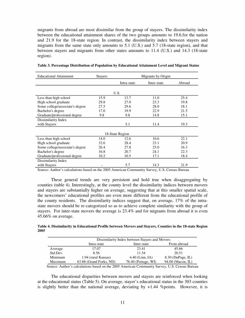
The spatial profiles shown above suggest that throughout the study region, and especially including the rural areas, newcomers are on average better educated than those already living in an area and that the educational gap differs by migrant origin. Figure 5 quantifies those differences, showing the distribution of stayers and movers across the five educational attainment levels. For comparative purposes, table 3 lists the educational profiles for the U.S. as a whole and the 18-state region. As a general trend, the well-educated are under-represented among the stayers and highly over-represented among the migrants. Moreover, the disparities are smaller for the nation as a whole than for the sampled 18-state region

0

5

10

15

20

25

30

35

1 2 3 4 1 2 3 4 1 2 3 4 1 2 3 4 1 2 3 4

1 = stayers; 2 = same-state movers; 3 = inter-state movers; 4 = from abroad

% Less than High School

High School

SomeCollege

Bachelor'sDegree

Grad./Prof.Degree

Figure 5. Percentage distribution of population by educational attainment levels and migrant status in the 18-state region

The mover-stayer differences are least pronounced when comparing stayers against

intra-state migrants. Compared to stayers, intra-state migrants are made up of a smaller share of persons with a high school degree or less, and a larger share of persons with some college or even a bachelor’s degree. The share of persons with a graduate or professional degree is about the same among the two groups.

The disparities between stayers and inter-state migrants are stark. In the U.S., 26.8% of the stayers have at least a bachelor’s degree compared to 37.7% of the inter-state migrants, yielding an educational gap between stayers and inter-state migrants of 10.9 percentage points. In the 18-state region, the percentage of inter-state movers with at least a bachelor’s degree exceeds 41% and the educational gap between inter-state migrants and stayers amounts to 14.2 percentage points.

An interesting distribution is observed for migrants from abroad: compared to stayers as well as to the two other migrant groups they have the largest share of persons without even a high school degree. But, they also have the second largest share of persons with at least a bachelor’s degree, and they rank first among all groups with respect to the share of persons with a graduate or professional degree. In fact, this more u-shaped distribution can be attributed to the heterogeneity of this group including, among others, low-skilled immigrants as well as the highly-skilled temporary workers with H-1B nonimmigrant visas. As a result,

11

migrants from abroad are most dissimilar from the group of stayers. The dissimilarity index between the educational attainment shares of the two groups amounts to 19.6.for the nation and 21.9 for the 18-state region. In contrast, the dissimilarity index between stayers and migrants from the same state only amounts to 5.1 (U.S.) and 5.7 (18-state region), and that between stayers and migrants from other states amounts to 11.4 (U.S.) and 14.3 (18-state region).

Table 3. Percentage Distribution of Population by Educational Attainment Level and Migrant Status

Educational Attainment Stayers Migrants by Origin

Intra-state Inter-state Abroad

U.S. Less than high school 15.9 13.7 11.0 25.4 High school graduate 29.8 27.0 23.3 19.8 Some college/associate's degree 27.5 29.6 28.0 18.1 Bachelor's degree 17.0 19.9 22.9 21.5 Graduate/professional degree 9.8 9.8 14.8 15.1 Dissimilarity Index with Stayers 5.1 11.4 19.3

18-State Region Less than high school 14.0 12.6 10.6 22.1 High school graduate 32.6 28.4 23.1 20.9 Some college/associate's degree 26.4 27.8 25.0 16.3 Bachelor's degree 16.8 20.7 24.1 22.3 Graduate/professional degree 10.2 10.5 17.1 18.4 Dissimilarity Index with Stayers - 5.7 14.3 21.9 Source: Author’s calculations based on the 2005 American Community Survey, U.S. Census Bureau

These general trends are very persistent and hold true when disaggregating by counties (table 4). Interestingly, at the county level the dissimilarity indices between movers and stayers are substantially higher on average, suggesting that at this smaller spatial scale, the newcomers’ educational profiles are even more different from the educational profile of the county residents. The dissimilarity indices suggest that, on average, 17% of the intra-state movers should be re-categorized so as to achieve complete similarity with the group of stayers. For inter-state movers the average is 23.4% and for migrants from abroad it is even 45.66% on average.

Table 4. Dissimilarity in Educational Profile between Movers and Stayers, Counties in the 18-state Region 2005

Dissimilarity Index between Stayers and Movers Intra-state Inter-state From abroad Average 17.07 23.41 45.66 Std.Dev. 8.56 11.54 20.51 Minimum 1.94 (rural Kansas) 4.40 (Linn, IA) 8.30 (DuPage, IL) Maximum 63.88 (Grand Forks, ND) 76.40 (Portage, WI) 94.00 (Macon, IL)

Source: Author’s calculations based on the 2005 American Community Survey, U.S. Census Bureau

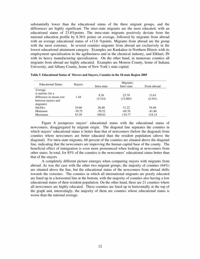
The educational disparities between movers and stayers are reinforced when looking at the educational status (Table 5). On average, stayer’s educational status in the 303 counties is slightly better than the national average, deviating by +1.44 %points. However, it is

12

substantially lower than the educational status of the three migrant groups, and the differences are highly significant. The inter-state migrants are the most educated, with an educational status of 23.8%points. The intra-state migrants positively deviate from the national education profile by 8.36% points on average, followed by migrants from abroad with an average educational status of +13.6 %points. Migrants from abroad are the group with the most extremes. In several counties migrants from abroad are exclusively in the lowest educational attainment category. Examples are Kankakee in Northern Illinois with its employment specialization in the agribusiness and in the chemical industry, and Elkhart, IN with its heavy manufacturing specialization. On the other hand, in numerous counties all migrants from abroad are highly educated. Examples are Monroe County, home of Indiana University, and Albany County, home of New York’s state capital. Table 5. Educational Status of Movers and Stayers, Counties in the 18-state Region 2005

Migrants: Educational Status Stayers Intra-state Inter-state From abroad Average (t-statistic for a difference in means test between stayers and migrants)

1.44 8.36 (5.214)

23.79 (12.085)

13.63 (4.541)

Std.Dev. 18.60 26.88 31.22 54.68 Minimum -39.75 -59.52 -69.76 -81.86 Maximum 43.39 100.61 110.77 118.14

Figure 6 juxtaposes stayers’ educational status with the educational status of

newcomers, disaggregated by migrant origin. The diagonal line separates the counties in which stayers’ educational status is better than that of newcomers (below the diagonal) from counties where newcomers are better educated than the resident population (above the diagonal). For intra-state migrants, 68 percent of the counties are situated above the diagonal line, indicating that the newcomers are improving the human capital base of the county. The beneficial effect of inmigration is even more pronounced when looking at newcomers from other states. In total, for 85% of the counties is the newcomers’ educational status better than that of the stayers.

A completely different picture emerges when comparing stayers with migrants from abroad. As was the case with the other two migrant groups, the majority of counties (64%) are situated above the line, but the educational status of the newcomers from abroad shifts towards the extremes. The counties in which all international migrants are poorly educated are lined up in a horizontal line at the bottom, with the majority of counties also having a low educational status of their resident population. On the other hand, there are 21 counties where all newcomers are highly educated. These counties are lined up in horizontally at the top of the graph and, interestingly, the majority of them are counties whose educational status is worse than the national average.

13

-82

-32

18

68

118

-60 -40 -20 0 20 40 60ES: stayers

ES: intrastate migrants

-82

-32

18

68

118

-60 -40 -20 0 20 40 60

ES: stayers

ES: interstate migrants

-82

-32

18

68

118

-60 -40 -20 0 20 40 60ES: stayers

ES: migrants from abroad

Figure 6. Relationship between educational status (ES) of stayers and newcomers, sampled counties 2005

14

3.4 Stock-Flow Relationships The previous section has shown that newcomers are, on average, better educated than

those who are already residents of the county, and that the differences are quite substantial for migrants moving in from other states. This section evaluates whether the education levels of the resident population (i.e., the stock) influences the education levels of the newcomers and whether such an effect is stronger in urban than in rural settings.

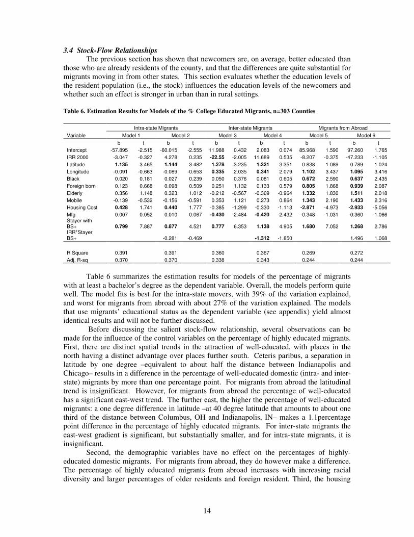
Table 6. Estimation Results for Models of the % College Educated Migrants, n=303 Counties

Intra-state Migrants Inter-state Migrants Migrants from Abroad Variable Model 1 Model 2 Model 3 Model 4 Model 5 Model 6

b t b t b t b t b t b t Intercept -57.895 -2.515 -60.015 -2.555 11.988 0.432 2.083 0.074 85.968 1.590 97.260 1.765 IRR 2000 -3.047 -0.327 4.278 0.235 -22.55 -2.005 11.689 0.535 -8.207 -0.375 -47.233 -1.105 Latitude 1.135 3.465 1.144 3.482 1.278 3.235 1.321 3.351 0.838 1.089 0.789 1.024 Longitude -0.091 -0.663 -0.089 -0.653 0.335 2.035 0.341 2.079 1.102 3.437 1.095 3.416 Black 0.020 0.181 0.027 0.239 0.050 0.376 0.081 0.605 0.672 2.590 0.637 2.435 Foreign born 0.123 0.668 0.098 0.509 0.251 1.132 0.133 0.579 0.805 1.868 0.939 2.087 Elderly 0.356 1.148 0.323 1.012 -0.212 -0.567 -0.369 -0.964 1.332 1.830 1.511 2.018 Mobile -0.139 -0.532 -0.156 -0.591 0.353 1.121 0.273 0.864 1.343 2.190 1.433 2.316 Housing Cost 0.428 1.741 0.440 1.777 -0.385 -1.299 -0.330 -1.113 -2.871 -4.973 -2.933 -5.056 Mfg 0.007 0.052 0.010 0.067 -0.430 -2.484 -0.420 -2.432 -0.348 -1.031 -0.360 -1.066 Stayer with BS+ 0.799 7.887 0.877 4.521 0.777 6.353 1.138 4.905 1.680 7.052 1.268 2.786 IRR*Stayer BS+ -0.281 -0.469 -1.312 -1.850 1.496 1.068 R Square 0.391 0.391 0.360 0.367 0.269 0.272 Adj. R-sq 0.370 0.370 0.338 0.343 0.244 0.244

Table 6 summarizes the estimation results for models of the percentage of migrants

with at least a bachelor’s degree as the dependent variable. Overall, the models perform quite well. The model fits is best for the intra-state movers, with 39% of the variation explained, and worst for migrants from abroad with about 27% of the variation explained. The models that use migrants’ educational status as the dependent variable (see appendix) yield almost identical results and will not be further discussed.

Before discussing the salient stock-flow relationship, several observations can be made for the influence of the control variables on the percentage of highly educated migrants. First, there are distinct spatial trends in the attraction of well-educated, with places in the north having a distinct advantage over places further south. Ceteris paribus, a separation in latitude by one degree –equivalent to about half the distance between Indianapolis and Chicago– results in a difference in the percentage of well-educated domestic (intra- and inter-state) migrants by more than one percentage point. For migrants from abroad the latitudinal trend is insignificant. However, for migrants from abroad the percentage of well-educated has a significant east-west trend. The further east, the higher the percentage of well-educated migrants: a one degree difference in latitude –at 40 degree latitude that amounts to about one third of the distance between Columbus, OH and Indianapolis, IN– makes a 1.1percentage point difference in the percentage of highly educated migrants. For inter-state migrants the east-west gradient is significant, but substantially smaller, and for intra-state migrants, it is insignificant.

Second, the demographic variables have no effect on the percentages of highly-educated domestic migrants. For migrants from abroad, they do however make a difference. The percentage of highly educated migrants from abroad increases with increasing racial diversity and larger percentages of older residents and foreign resident. Third, the housing

15

variables have a mixed impact on the percentage of highly educated migrants. An increase in the percentage of mobile homes surprisingly increases the percentage of highly educated from abroad. A high percentage of homeowners paying less than 30% of their income on housing related costs (low costs of living) decreases the influx of highly educated from abroad but increases the inflow of highly-educated intra-state migrants. The housing variables have no influence on the inflow of college-educated inter-state migrants. Fourth, the industrial structure only affects interstate migrants. The share of manufacturing employment is inversely related to the influx of college-educated interstate migrants.

Turning now to the stock-flow relationships shown for models 1, 3, and 5, the estimation results convey a clear message. The more educated the resident population, the more educated the newcomers. The effect is strongest for migrants from abroad. A one point increase in the percentage of college-educated stayers increases the percentage of college-educated migrants from abroad by 1.68 points. For domestic migrants, the effect is substantially lower, only amounting to 0.799 points for both intra-state migrants and 0.77 for inter-state migrants.

To demonstrate the implied impacts on human capital accumulation, consider a very simplified scenario. Assume that at t=0 a county has 11,000 residents of which 3000 (27.3%) are highly-educated residents. Assume further that the county receives 800 migrants per year, 37.5% of which are highly educated, that there is no outmigration (or that outmigration rates do not vary by educational status). If there is no stock-flow relationship, i.e., bStayerBS+=0 then the stock of highly educated residents will increase8 and after 10 years, 31.5 percent of the residents will be college-educated. If bStayerBS+=0.77 (inter-state migrants) then the human capital accumulation occurs more rapidly. The benchmark of 31.5% college-educated residents is already reached after 7½ years. If bStayerBS+=1.68 (migrants from abroad), it will only take 6½ years before the population has 31.5 percent college-educated residents.

Models 2, 4, and 6 address the question whether the self-perpetuating human capital accumulation is independent of the degree of rurality. For intra-state migrants the degree of rurality has no effect on the proportion of college-educated in-migrants, neither as an independent effect nor in combination with the share of college-educated stayers. The same is true for migrants from abroad.

For inter-state migrants, however, a different situation emerges. Model 3 suggests that the percentage of college-educated migrants decreases with increases rurality. The expanded Model 4, which includes the rurality variable as well as the interaction between rurality and the stock variable (Stayer BS+), suggests that rurality does not have an independent effect but instead modifies the influence of the stock variable on the inflow of newcomers. As hypothesized, education of the resident population (i.e., the stock) positively affects the education levels of inter-state migrants, but the size of the effect diminishes significantly9 with increasing rurality.

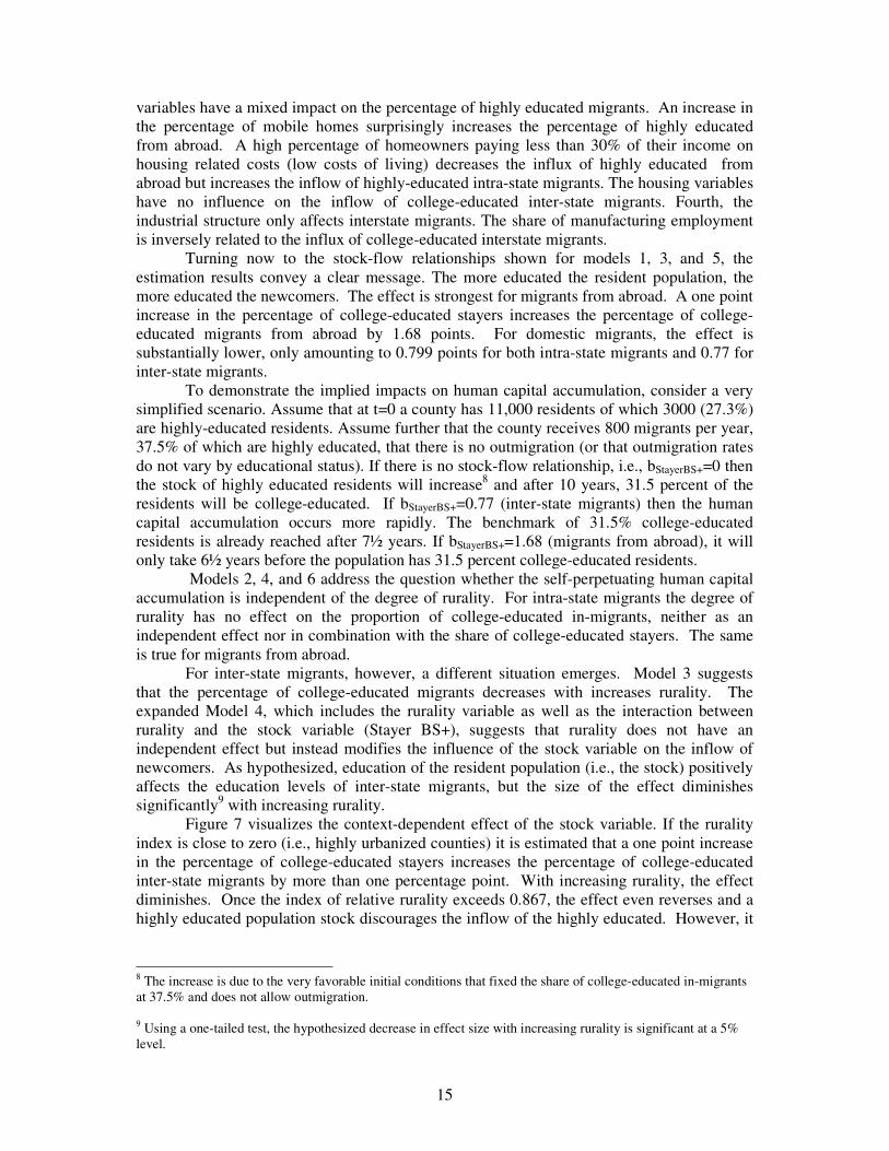
Figure 7 visualizes the context-dependent effect of the stock variable. If the rurality index is close to zero (i.e., highly urbanized counties) it is estimated that a one point increase in the percentage of college-educated stayers increases the percentage of college-educated inter-state migrants by more than one percentage point. With increasing rurality, the effect diminishes. Once the index of relative rurality exceeds 0.867, the effect even reverses and a highly educated population stock discourages the inflow of the highly educated. However, it

8 The increase is due to the very favorable initial conditions that fixed the share of college-educated in-migrants at 37.5% and does not allow outmigration. 9 Using a one-tailed test, the hypothesized decrease in effect size with increasing rurality is significant at a 5% level.

16

should be noted that the threshold at which the effect is reversed falls outside the sample range.

-0.2

0.0

0.2

0.4

0.6

0.8

1.0

1.2

0.0 0.1 0.2 0.3 0.4 0.5 0.6 0.7 0.8 0.9 1.0

Index of Relative Rurality

Effe

ct S

ize

------------- Sampled Range -------------

Model 3

Model 4

Figure 7. The effect of the percentage of college-educated stayers on the percentage of college-educated inter-state migrants.

4. Summary and Conclusion

A knowledge–based workforce is a necessary albeit not sufficient condition for successful competition in today’s economy. This paper thus aimed at contributing to our understanding of changes in the accumulation of intellectual capital. The paper addressed several core questions. Does the education level of newcomers vary systematically vary over space? Are newcomers, on average, better educated than those already living in an area and does the educational gap differ by migrant origin? Does educational deprivation of a region’s population (stock) dampen the inflow of the well-educated and if so, is the effect higher in urban than in rural areas? The empirical analysis is based on data from the 2005 American Community Survey and includes a sample of 303 counties/rural areas from 18 states. Several key results can be extracted from the analysis. First, newcomers are significantly and substantially better educated than the resident population. Second, the education gap is most pronounced for newcomers from other states. Third, migrants’ educational status varies systematically across space. Domestic migrants are better educated in the northern than in the southern counties. For inter-state migrants and migrants from abroad, education levels diminish from East to West. Fourth, when accounting for the variation in the educational status of newcomers, the educational status of the resident population turns out to be the most powerful predictor. A well-educated stock positively influences the educational status of the migrant population. Finally, for the interstate migrants this stock-flow relationship is context dependent: the power of a well-educated stock to attract well-educated migrants is quite forceful in urban settings, but diminishes with increasing rurality. The implications are obvious: if these trends continue then areas with a well-educated population will attract more educated people. As a result, the spatial distribution of the highly educated population will become increasingly concentrated, creating disparities between brain-rich and brain-poor regions. Of course, this poses severe challenges for regions already lagging behind as they are at high risk of being further left behind. Yet, the implied future developments also offer promising opportunities for emerging knowledge agglomerations, with a prospect for sustained growth of its human capital base.

Future research will proceed along two avenues. First, while this research looks at the inflow of newcomers, attention should also be paid to the outflow. The sorting process implied by the results of this study will be even more intense in counties where those who enter also have a better educational status than those who leave. Second, the research should

17

be expanded to include a temporal component, so as to better assess the persistence and speed of the population sorting.

References Austin, J. and B. Affolter-Caine 2006. The Vital Center: A Federal-State Compact to Renew

the Great Lakes Region. The Brookings Institution Metropolitan Policy Program.http://media.brookings.edu/mediaarchive/pubs/metro/pubs/20061020_RenewGreatLakes.pdf

Basker, E. 2002. Education, Job Search and Migration. University of Missouri-Columbia Working Paper No. 02-16. http://papers.ssrn.com/sol3/papers.cfm?abstract_id=371120#PaperDownload

Clark, T.N., Lloyd, R., Wong, K., Jain, P. 2002. Amenities Drive Urban Growth. Journal of Urban Affairs 24(5): 493-515.

Cooke, P. 2002. Knowledge Economies. London: Routledge. Costa, D.L. and M.E. Kahn 2000. Power Couples: Changes in the Locational Choice of the

College Educated, 1940–1990, The Quarterly Journal of Economics 115(4): 1287–1315.

Duncan O.D., Duncan B. (1955) A methodological analysis of segregation indexes, American Sociological Review, 41, 210–217.

Florida R. 2002a. Bohemia and economic geography. Journal of Economic Geography 2: 55-71.

Florida, R. 2002b.The Rise of the Creative Class. New York, NY: Basic Books. Franklin, R. S. 2003. Migration of the Young, Single, and College Educated: 1995–2000.

Census 2000 Special Reports CENSR–12. Greunz, L. 2004.Interregional Knowledge Spillovers in Europe.In: Knowledge Spillovers and

Knowledge Management, eds.: C. Karlsson, P. Flensburg and S.–A. Hörte. Cheltenham UK, Northampton, MA, USA: Edward Elgar, pp. 110–135.

Glaeser, E.L., Kolko, J., Saiz, A.. 2000.Consumer City. NBER Working Paper Series # 7790..

Henderson, J. and B. Abraham 2004. Can Rural America Support a Knowledge Economy? Federal Reserve Bank of Kansas City – Economic Review. Third Quarter 2004.

Karlsson, C., P. Flensburg, and S.–A. Hörte 2004. Introduction: knowledge spillover and knowledge management. In: Knowledge Spillovers and Knowledge Management, eds.: C. Karlsson, P. Flensburg and S.–A. Hörte. Cheltenham UK, Northampton, MA, USA: Edward Elgar, pp. 3–34.

Kodrzycki, Y. 2001. Migration of Recent College Graduates: Evidence from the National Longitudinal Survey of Youth. New England Economic Review 2001: 13-34.

Lichter, D., D. McLaughlin and G. Cornwell 1992. Migration and the Loss of Human Resources in Rural America. In: Investing in People: The Human Capital Needs of Rural America, eds.: L. Beaulieu and D. Mulkey. Boulder, Westview.

McCann P. and S. Sheppard 2002. Human capital, higher education and graduate migration: an analysis of Scottish and Welsh students. Unpublished paper.

Mathur, V. 1999. Human Capital-Based Strategy for Regional Economic Development. Economic Development Quarterly 13(4): 203-21

Munnich, L.W., Schrock, G. and K. Cook 2002. Rural Knowledge Clusters: The Challenge of Rural Economic Prosperity. Reviews of Economic Development Literature and Practice, No. 12.

Purdue Center for Regional Development and Indiana Business Research Center 2007. Unlocking Regional Competitiveness: The Role of Industry Clusters. http://www.ibrc.indiana.edu/innovation/reports.html

18

Ritsilä, J. and M. Haapanen 2003. Where Do the Highly Educated Migrate? Micro–Level Evidence from Finland. International Review of Applied Economics17( 4): 437 – 448.

Schachter, J.P., R.S. Franklin and M.J.Perry 2003. Migration and Geographic Mobility in Metropolitan and Non–metropolitan America: 1995–2000. Census 2000 Special Reports CENSR–12.

Waldorf, B. 2006a. No County Left Behind? The Persistence of Educational Deprivation in Indiana. Purdue Center for Regional Development, Purdue University, Research Paper. PCRD-R-2. http://www.ces.purdue.edu/extbusiness/pcrd/PCRD-R-2LR.pdf

Waldorf, B. 2006b. A continuous multi-dimensional measure of rurality: Moving beyond threshold measures. Selected Paper, Annual Meetings of the Association of Agricultural Economics, July 2006, Long Beach, California. http://agecon.lib.umn.edu/cgi-bin/pdf_view.pl?paperid=21522&ftype=.pdf

Waldorf, B. 2007. The Emergence of a Knowledge Agglomeration: A Spatial-temporal Analysis of Intellectual Capital in Indiana. In: Poot, J., B. Waldorf and L. van Wissen (eds). Migration and Human Capital. Edward Elgar, forthcoming.

Whisler, R., B. Waldorf, G. Mulligan and D.Plane 2007. Quality-of-Life and Migration of the Highly-Educated: A Demographic Segmentation Approach. Working Paper.

Appendix: Estimation Results for Models of the Migrants’ Educational Status, n=303 Counties

Intra-state Migrants Inter-state Migrants Migrants from Abroad

Variable Model 7 Model 8 Model 9 Model 10 Model 11 Model 12 b t b t b t b t b t b t

Intercept -91.097 -2.239 -92.722 -2.273 -3.281 -0.068 -7.452 -0.155 150.388 1.646 153.641 1.677IRR 2000 -7.759 -0.442 -8.455 -0.481 -45.930 -2.207 -47.717 -2.294 -16.144 -0.409 -14.750 -0.373Latitude 1.797 2.915 1.845 2.971 2.408 3.292 2.531 3.446 2.275 1.642 2.179 1.561Longitude -0.104 -0.412 -0.105 -0.414 0.555 1.850 0.554 1.849 1.954 3.437 1.955 3.436Black 0.013 0.063 0.035 0.168 -0.010 -0.041 0.047 0.189 0.866 1.864 0.821 1.745Foreign born 0.227 0.667 0.177 0.507 0.181 0.450 0.052 0.127 1.421 1.859 1.522 1.944Elderly 0.645 1.080 0.573 0.945 -0.410 -0.578 -0.594 -0.827 2.401 1.790 2.545 1.867Mobile -0.321 -0.655 -0.361 -0.732 1.095 1.883 0.991 1.696 2.973 2.700 3.054 2.751Housing Cost 0.644 1.399 0.672 1.453 -0.295 -0.541 -0.222 -0.407 -5.015 -4.849 -5.072 -4.879Mfg -0.408 -1.500 -0.407 -1.494 -0.869 -2.692 -0.866 -2.686 -0.607 -0.993 -0.610 -0.997ES stayer 0.683 6.900 0.792 4.249 0.736 6.269 1.016 4.608 1.307 5.874 1.088 2.599IRR*ES stayer -0.383 -0.690 -0.985 -1.637 0.767 0.615 R Square 0.368 0.369 0.341 0.346 0.229 0.230Adj. R-sq 0.346 0.345 0.318 0.321 0.203 0.201