Brief guide to instructors

TUTORIALS IN UPPER DIVISION

Last updated Summer 2011

Please feel free to add comments and improve this document.

Week by week materials available in the "Tutorials" folder at

http://www.colorado.edu/sei/departments/physics_3310.htm

http://www.colorado.edu/sei/departments/physics_3220.htm

What are tutorials? Tutorials are weekly student sessions, modeled after research-validated curricula developed at the University of Washington. UW Tutorials are largely for the introductory level, but now also exist in upper-division Quantum Mechanics. They are designed to change the way study sessions/recitation sections work: from teacher-centered to student-centered. Students work in small groups, and the role of the instructor becomes that of a learning coach. Materials are designed to target known student difficulties, to elicit and develop conceptual understanding and math/physics connections. They also serve as a powerful tool to help faculty listen in on student reasoning, to get a clearer sense of student ideas, and where they are still struggling.

What is the pedagogical theory behind tutorials? Education research indicates that passive learning, in which students listen to an expert explain ideas, is rarely as effective as active learning, in which the responsibility for learning is shifted to the students. Tutorials are designed to shift the focus of learning to the students, a "constructivist" view of education. Tutorials often follow an "elicit-confront-resolve" cycle. The Tutorial guides them through logical steps, encouraging them to utilize multiple representations, confront possible internal inconsistencies in their initial beliefs, and to make sense of topics which might otherwise appear purely formal. Tutorials place a large emphasis on the process of problem solving - eliciting conflicting ideas, encouraging discussion and debate, requiring explanation and consistency rather than merely "answers". They tend to focus on powerful and common pre-conceptions. UW Quantum materials build on student interviews and extensive pre-post testing. At Colorado, we are just starting this process for E&M (and a few additional Quantum) Tutorials.

Are tutorials effective? The tutorials are highly rated by students, who indicate that this is something they would be disappointed to see dropped from the course. They indicate that tutorials are fun and engaging and an opportunity to think about the ideas brought up in lecture. Instructors are very positive about the tutorials as well, and find that they offer opportunities to gain a window into student thinking not typically available. Our studies have shown that, even when the effects of background preparation (such as GPA in prior courses) is taken into account, tutorial attendance has a positive effect on students’ conceptual understanding of E&M course material. See PERC 2011 paper by Chasteen, in Publications, for full information.

Running Tutorials: You will want a room with small tables for four. Groups should be given a white board and markers. This allows students to easily communicate their ideas to each other and with the Learning Assistant (LA) or instructor. Tutorials take approximately an hour, but many students won't finish. Advise students that this is voluntary, they will not be required to turn in the tutorial. However, it would be in their interest to fill things out as completely as possible, since many of the topics will also be covered on the homework. Group members are encouraged to work together, and the instructor(s) wander from group to group to see if anyone is completely lost/stuck. Trust the students - they can figure this stuff out on their own. Allow space for them to be wrong (as long as they are still "self-correcting"), try to stay away as long as they are working productively - use this as an opportunity to listen to student ideas. I tell my students “we will try our hardest not to give you any of the answers, but we will also try our hardest to make sure you figure everything out for yourself.”

Where can I go to learn more?

Stephanie Chasteen and S. Pollock, "Transforming Upper-Division Electricity and Magnetism", 2008 PERC proceedings, can be found at per.colorado.edu/research/papers_author.htm#stephanie_chasteen

Stephanie Chasteen,"Teasing out the effect of tutorials via multiple regression", 2011 PERC proceedings, can be found at per.colorado.edu/research/papers_author.htm#stephanie_chasteen

E. Redish: Teaching Physics with the Physics Suite. Can be found free at http://www2.physics.umd.edu/~redish/Book/

Lillian McDermott's Millikan Lecture: “How We Teach and How Students Learn - A mismatch?” AJP 61, ('93),  295 (http://unr.edu/homepage/jcannon/ejse/mcdermott.html)

Pre semester logistics for running tutorials at CU:

1) You must arrange a time and a place for the Tutorials. We have established an optional 1-credit "coseminar" course (Phys 3311 for E&M, Phys 3221 for Quantum), you need to discuss with the undergraduate coordinator (Leigh Dodd) so the course is listed as active for the semester. The deadline is the end of February for the Fall semester, and the end of September for the Spring semester. This will get this onto the CU registration system for your term, and you will also want to add a comment to your regular course registration page to let the students know about it. (The co-sem is 1 credit, pass/fail, and does NOT count in any way towards the Physics major. So far, it has been treated as completely optional, just an opportunity for students, not a requirement)

Tutorials have run on Fridays in the Tutorial Bays, with homeworks due Wednesday. In E&M, conflicts with Junior Lab and other core courses have restricted the timing for tutorials to Fridays between 3 and 5. The idea is that the Tutorial is a starting point for the upcoming homework, which is sufficiently far away that students will not be focused on those particular problems. This is not a homework study session, but it is targeted to help facilitate the upcoming assignment. The materials usually work best if they come after some treatment in your class.

2) You must arrange for a Learning Assistant. The physics department will pay one undergraduate $1500/term for ~6-8 hrs/week (they also must sign up for a special pedagogy seminar in the School of Ed). We solicit applications midway through the previous term, your participation is welcome, but not required (Just let Steve Pollock and/or Mike Dubson know you're looking for an LA). The LA will run sessions, but must also spend time before the Tutorials reviewing the material (some of that time with you!) and should spend time afterwards reflecting on issues they encountered.

Plan on spending regular time every week with your LA - they will be a great help to you, but they are still just undergraduates who have probably just gone through this course themselves. They may also be thinking about teaching as a career - be aware that you are supporting this interest.

4) Mention the Tutorials and their purpose in your syllabus and first class(es)

5) Consider using class time for a post-test in class at the end of the term, and also consider giving a pre-test for about 1/3 of the first or second lecture. (See S. Chasteen or S. Goldhaber for details)

6) Download all Tutorial materials for the semester:

http://www.colorado.edu/sei/departments/physics_3310.htm

http://www.colorado.edu/sei/departments/physics_3220.htm

and make sure you can read/print them ok.

Week before classes start

1) Be sure you have whiteboards, pens, and erasers (or tissue), and snacks (if you wish).

2) Arrange a regular time (1 hr /week) to meet with your LA, probably a few days before each Tutorial, to go over materials, discuss issues, and help orient them. This will be your "prep" session (and should suffice for both you and the LA!)

Every week during the term:

1) Look over our online instructors manual for the upcoming Tutorial! Check out in advance of your prep meeting if you need demos/equipment/photocopies: make sure it's all there and in order (or have the LA take care of this)

2) I suggest you do each Tutorial in advance, write out your answers. Think about student misconceptions, why is the Tutorial "hammering" on certain things? What sorts of questions will help students make sense of this if they're struggling? If Tutorial questions are ambiguous (sometimes intentional!) think about what they're after, so you can guide the LA (and later, the students). Ask SJP about research behind the Tutorials if you're curious or confused about what the point of some of the tutorial activities. Some instructor manuals for individual tutorials are available for 3310.

3) Announce the tutorial in-class that day, perhaps as a clicker question (“Do you plan to go to today’s tutorial on XXX”?) to encourage participation.

4) If you're feeling generous, buy some snacks for your students. Food is a great social facilitator!

5) After the Tutorial, if you have suggestions or comments, write them or email them (to Steven Pollock) immediately, before you forget. If you want to re-design any materials, feel free, please let us know what you're doing so your hard work doesn't get lost.

History:

3310 (E&M) Tutorials:

Sp 2008, S. Pollock (with LA: Darren Tarshis, SEI Postdoc: Stephanie Chasteen)

Fa 2008: Mike Dubson and Ed Kinney

Sp 2009: Ed Kinney (LA: Markus Atkinson)

Fa 2009: Thomas Schibli

Sp 2010: Oliver DeWolf

3220 (Quantum) Tutorials:

Fa 2008: S. Pollock, Oliver Dewolfe (with SEI Postdoc: Steven Goldhaber)

Sp 2009: O. Dewolfe (LA: Markus Atkinson)

Fa 2009: Andreas Becker

Sp 2010: Murray Holland

Fa 2010: Chuck Rogers

Sp 2011: Andreas Becker

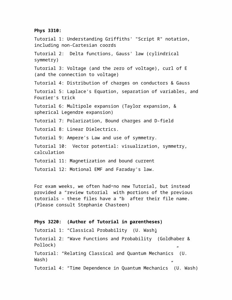
Phys 3310:

Tutorial 1: Understanding Griffiths' "Script R" notation, including non-Cartesian coords

Tutorial 2: Delta functions, Gauss' law (cylindrical symmetry)

Tutorial 3: Voltage (and the zero of voltage), curl of E (and the connection to voltage)

Tutorial 4: Distribution of charges on conductors & Gauss

Tutorial 5: Laplace's Equation, separation of variables, and Fourier's trick

Tutorial 6: Multipole expansion (Taylor expansion, & spherical Legendre expansion)

Tutorial 7: Polarization, Bound charges and D-field

Tutorial 8: Linear Dielectrics.

Tutorial 9: Ampere's Law and use of symmetry.

Tutorial 10: Vector potential: visualization, symmetry, calculation

Tutorial 11: Magnetization and bound current

Tutorial 12: Motional EMF and Faraday's law.

For exam weeks, we often had no new Tutorial, but instead provided a “review tutorial” with portions of the previous tutorials – these files have a “b” after their file name. (Please consult Stephanie Chasteen)

Phys 3220: (Author of Tutorial in parentheses)

Tutorial 1: “Classical Probability” (U. Wash)

Tutorial 2: “Wave Functions and Probability” (Goldhaber & Pollock)

Tutorial: “Relating Classical and Quantum Mechanics” (U. Wash)

Tutorial 4: “Time Dependence in Quantum Mechanics” (U. Wash)

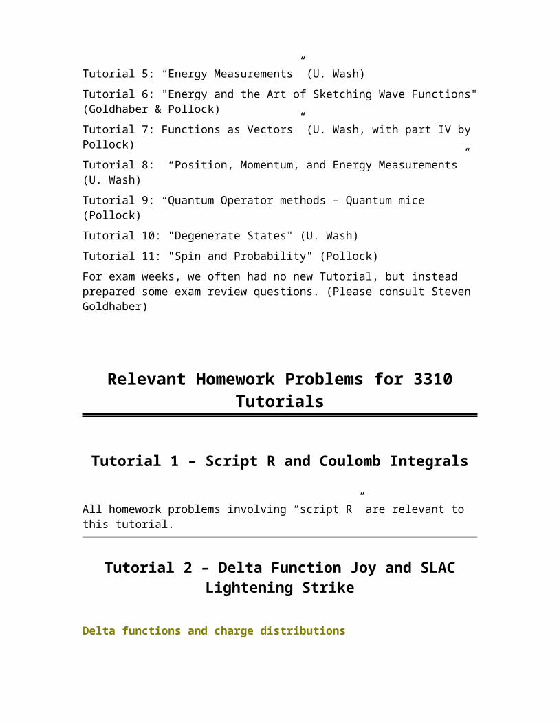
Tutorial 5: “Energy Measurements” (U. Wash)

Tutorial 6: "Energy and the Art of Sketching Wave Functions" (Goldhaber & Pollock)

Tutorial 7: Functions as Vectors” (U. Wash, with part IV by Pollock)

Tutorial 8: “Position, Momentum, and Energy Measurements” (U. Wash)

Tutorial 9: “Quantum Operator methods – Quantum mice (Pollock)

Tutorial 10: "Degenerate States" (U. Wash)

Tutorial 11: "Spin and Probability" (Pollock)

For exam weeks, we often had no new Tutorial, but instead prepared some exam review questions. (Please consult Steven Goldhaber)

Relevant Homework Problems for 3310 Tutorials

Tutorial 1 – Script R and Coulomb Integrals

All homework problems involving “script R” are relevant to this tutorial.

Tutorial 2 – Delta Function Joy and SLAC Lightening Strike

Delta functions and charge distributions

a) On the previous homework we had two point charges: +3q located at x=-D, and -q located at x=+D.

Write an expression for the volume charge density (r) of this system of charges.

b) On the previous homework we had another problem with a spherical surface of radius R (Fig 2.11 in Griffiths) which carried a uniform surface charge density . Write an expression for the volume charge density (r) of this charge distribution. (Hint: use spherical coordinates, and be sure that your total integrated charge comes out right.)

(Verify explicitly that the units of your final expression are correct)

c) Suppose a linear charge density is given to you as

€

λ(x) = q0δ(x) + 4q0δ(x −1)Describe in words what this charge distribution looks like.

How much total charge do we have?

Assuming that q0 is given in Coulombs, what are the units of all other symbols in this equation (including, specifically the symbols λ, x, the delta function itself, the number written as "4" in front of the second term, and the number written as "1" inside the last function.

It can also be tricky to translate between the math and the physics in problems like this, especially since the idea of an infinite charge density is not intuitive. Practice doing this translation is important (and not just for delta functions!)

Electric field of coaxial cable

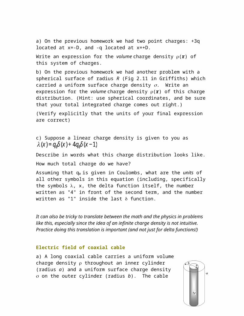
a) A long coaxial cable carries a uniform volume charge density throughout an inner cylinder (radius a) and a uniform surface charge density on the outer cylinder (radius b). The cable is overall electrically neutral. Find E everywhere in space, and sketch it.

b) Last week you considered how much charge a child's balloon might hold before sparking. Now let's consider the same question for a real life coax cable. Making any reasonable guess as to physical dimensions for a cable like one that might attach your stereo to your TVs - what would be the maximum static charge you could put onto that cable?

(This is estimation - I don't care if you're off by a factor of 2, or even 10, but would like to know the rough order of magnitude of the answer!) From where to where do you expect a spark to go, if it does break down?

Tutorial 3 – E Fields and Potentials

Divergence and Curl

Consider an electric field E =

€

cr r r2 (Please note the numerator is not

€

ˆ r : this is NOT the

usual E field from a point charge at the origin, which would give

€

c'r r r3 , right?!)

a) - Calculate the divergence and the curl of this E field.

- Explicitly test your answer for the divergence by using the divergence theorem.

(Is there a delta function at the origin like there was for a point charge field, or not?)

- Explicitly test your answer for the curl by using the formula given in Griffiths problem 1.60b, page 56.

b) What are the units of c? What charge distribution would you need to produce an E field like this? Describe it in words as well as formulas. (Is it physically realizable?)

Allowed E fields

Which of the following two static E-fields is physically impossible. Why?

i)

€

E = c(2xˆ i − x ˆ j + y ˆ k )

ii)

€

E = c(2xˆ i + z ˆ j + y ˆ k )

where c is a constant (with appropriate units)

For the one which IS possible, find the potential V(r), using the origin as your reference point (i.e. setting V(0)=0)

- Check your answer by explicitly computing the gradient of V.

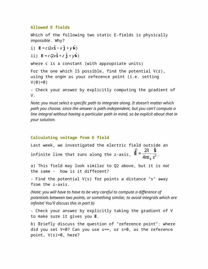
a b

-

+

Note: you must select a specific path to integrate along. It doesn't matter which path you choose, since the answer is path-independent, but you can't compute a line integral without having a particular path in mind, so be explicit about that in your solution.

Calculating voltage from E field

Last week, we investigated the electric field outside an infinite line that runs along the z-

axis,

€

E = 2λ

4πε0

r s s2 .

a) This field may look similar to Q2 above, but it is not the same - how is it different?

- Find the potential V(s) for points a distance "s" away from the z-axis.

(Note: you will have to have to be very careful to compute a difference of potentials between two points, or something similar, to avoid integrals which are infinite! You'll discuss this in part b)

- Check your answer by explicitly taking the gradient of V to make sure it gives you E.

b) Briefly discuss the question of "reference point": where did you set V=0? Can you use s=∞, or s=0, as the reference point, V(s)=0, here?

- How would your answer change if I told you that I wanted you to set V=0 at a distance s=3 meters away from the z-axis?

- Why is there trouble with setting V(∞)=0? (our usual choice), or V(0)=0 (often our second choice).

c) A typical Colorado lightning bolt might transfer a few Coulombs of charge in a stroke. Although lightning is clearly not remotely "electrostatic", let's pretend it is - consider a brief period during the stroke, and assume all the charges are fairly uniformly distributed in a long thin line. If you see the lightning stroke, and then a few seconds later hear the thunder, make a very rough estimate of the resulting voltage difference across a distance the size of your heart. (For you to think about - why is this not worrisome?)

What's the model? I am thinking of a lightning strike as looking rather like a long uniform line of charge... You've done the "physics" of this in the previous parts! (But e.g., you need a numerical estimate for λ. How long might that lightning bolt be? For estimation problems, don't worry about the small details, you can be off by 3, or even 10, I just don't want you off by factors of 1000's!)

Tutorial 4 – Conceptually Understanding Conductors

Gauss’s law and conductors

Griffiths 2.35 (p. 101)

Gauss’s law and cavities

Griffiths 2.36 (p. 101)

Please be sure to explain your reasoning on all parts, and add to this the problem the following:

In part a, be sure to sketch the charge distribution.

In part c, sketch the E fields (everywhere in the problem, i.e. in the cavities and also outside the big sphere)

f) Lastly - if someone moved qa a little off to one side, so it was no longer at the center of its little cavity, which of your answers would change? Please explain.

I really like this problem, lots of good physics in it! Try to think it through carefully, make physical sense of all your answers, don't just take someone else's word for it! ‘’

Tutorial 5 – Separation of Variables

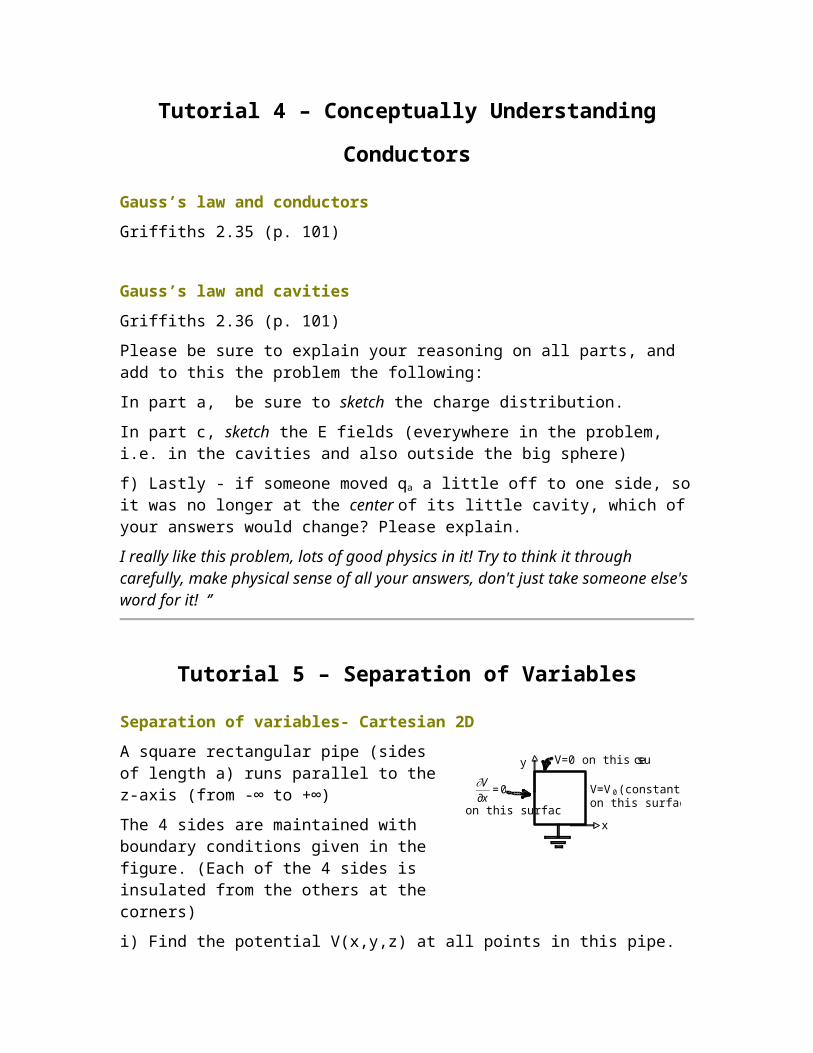
Separation of variables- Cartesian 2D

A square rectangular pipe (sides of length a) runs parallel to the z-axis (from -∞ to +∞)

The 4 sides are maintained with boundary conditions given in the figure. (Each of the 4 sides is insulated from the others at the corners)

i) Find the potential V(x,y,z) at all points in this pipe.

ii) Sketch the E-field lines and equipotential contours inside the pipe. (Also, state in words what the boundary condition on the left wall means - what does it tell you? Is the left wall a conductor?)

iii) Find the charge density (x,y=0,z) everywhere on the bottom conducting wall (y=0).

Separation of variables- Cartesian 3D

You have a cubical box (sides all of length a) made of 6 metal plates which are insulated from each other.

The left wall is located at x=-a/2,the right wall is at x=+a/2.

V=V0

y

z

x

V=V0 +a

+a/2 +a

-a/2

V=0 on this surface

€

∂V∂x

= 0 on this surface

V=V0 (constant) on this surface

x

y

Both left and right walls are held at constant potential V=V0.

All four other walls are grounded.

(Note that I've set up the geometry so the cube runs from y=0 to y=a, and from z=0 to z=a, but from x=-a/2 to x=+a/2 This should actually make the math work out a little easier!)

Find the potential V(x,y,z) everywhere inside the box.

(Also, is V=0 at the center of this cube? Is E=0 there? Why, or why not?)

Separation of Variables: Spherical

The potential on the surface of a sphere (radius R) is given by V=V0 cos(2).

(Assume V(r=∞)=0, as usual. Also, assume there is no charge inside or outside, it's ALL on the surface!)

i) Find the potential inside and outside this sphere.

(Hint: Can you express cos(2) as a simple linear combination of some Legendre polynomials? )

ii) Find the charge density on the sphere.

Tutorial 6 – Separation of Variables & Multipole

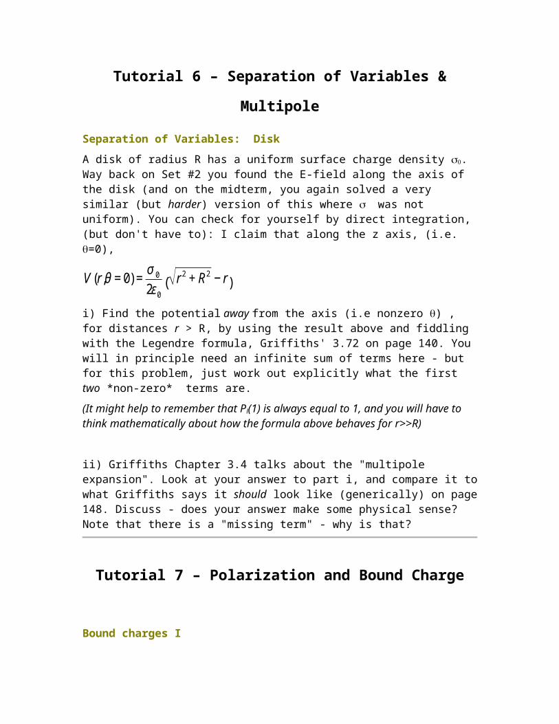
Separation of Variables: Disk

A disk of radius R has a uniform surface charge density . Way back on Set #2 you found the E-field along the axis of the disk (and on the midterm, you again solved a very similar (but harder) version of this where was not uniform). You can check for yourself by direct integration, (but don't have to): I claim that along the z axis, (i.e. =0),

€

V (r,θ = 0) = σ 0

2ε0

r2 + R2 − r( )

i) Find the potential away from the axis (i.e nonzero ) , for distances r > R, by using the result above and fiddling with the Legendre formula, Griffiths' 3.72 on page 140. You will in principle need an infinite sum of terms here - but for this problem, just work out explicitly what the first two *non-zero* terms are.

(It might help to remember that Pl(1) is always equal to 1, and you will have to think mathematically about how the formula above behaves for r>>R)

ii) Griffiths Chapter 3.4 talks about the "multipole expansion". Look at your answer to part i, and compare it to what Griffiths says it should look like (generically) on page 148. Discuss - does your answer make some physical sense? Note that there is a "missing term" - why is that?

Tutorial 7 – Polarization and Bound Charge

Bound charges I

Consider a long insulating rod, (a dielectric cylinder), radius a. Suppose that the rod has no free charge but has a permanent polarization P(s,,z) = C s (= ˆCss ), where s is the usual cylindrical radial vector from the z-axis, and C is a positive constant). Neglect end effects: the cylinder is long. Note that this rod is NOT a linear dielectric. Only very special materials can have a permanent polarization. Bariam titanate, BaTiO3 , is one such material. A rod with a permanent polarization is called an "electret".

A) Calculate the bound charges b and b (on the surface, and interior of the rod respectively). What are the units of C? Sketch the charge distribution of the rod.

B) Next, use these bound charges (along with Gauss' law) to find the electric field inside and outside the cylinder. (Direction and magnitude)

C) Find the electric displacement field D inside and outside the cylinder, and verify that "Gauss's Law for D" (Eqn 4.23, p. 176) works.

Bound charges II

Consider now a hollow insulating rod, with inner radius a and outer radius b.

Suppose now that the rod has a different permanent polarization, namely P(s,,z) =

2

C ˆs

s for a < s < b , C = positive constant (not the same constant as in Q1 ). Again, this

is not an ordinary linear dielectric. It has a permanent polarization.

A) We have vacuum for s < a and s > b. What does that tell you about P in those regions? Find the bound charges b and b (b on the inner AND outer surfaces of the hollow rod, and b everywhere else. Use these bound charges, along with Gauss' law, to find the electric field everywhere in space. (Direction and magnitude)

B) Use Griffiths' Eq 4.23 (p. 176) to find D everywhere in space. (This should be quick - are there any free charges in this problem?) Use this (simple) result for D (along with Griffiths basic definition/relation of E to D, Eq 4.21) to find E everywhere in space. (This should serve as a check for part a, and shows why sometimes thinking about D fields is easier and faster!)

Tutorial 8 – Spherical Linear Dielectric

Griffiths questions 4.36 (p.199)

Cylindrical capacitor, bound charges

CALCULATION (from deGrand)

(a) Find the capacitance per unit length of a long cylinder with an inner conductor of radius a, an outer conductor of inner radius b and outer radius c, a material with dielectric constant K in between, and a free charge per unit length λ on each conductor (of opposite signs on either). (b) What and where are the polarization charges?

Dielectric series capacitor 1

CALCULATION (deGrand)

The dielectric series capacitor is a parallel place capacitor of surface area A and thickness , between which a dielectric slab of thickness d1 and constant K1 and a

dielectric slab of thickness d2 and constant K2 are inserted. Assume free charges on the top and bottom of . Find (a) in each slab (b) in each slab (c) in each slab (d) the potential between the plates (e) the location and the value of all bound charges (f) the capacitance.

Dielectric series capacitor 2

CALCULATION (deGrand)

The dielectric series capacitor is a parallel place capacitor of width w, depth l, and thickness d, between which a dielectric slab of constant K is inserted for a width s (see figure). We put a voltage V between the plates. Find [4 points each] (a) in each slab (b) in each slab (c) the free charge density in each region (d) the bound surface charge density in each region (e) the capacitance. Neglect all fringing fields in your calculations.

Question 1 Dielectric sphere

GAUSS’ LAW; CALCULATION (U. Nauenberg, solutions available)

A sphere of radius “R” is made up of a dielectric material with dielectric

constant eispolon̨ and contains a uniform free charge density per unit volume ρf .

Show that the potential at the center is given by:

Question 2 Dielectric sphere in E field

CALCULATION; BOUNDARY VALUE (U. Nauenberg, HW8, solutions available)

A solid dielectric sphere of radius “a”, with dielectric constant epsilon̨, has

a uniform free surface charge/unit area σ is placed in an initially uniform

electric field E0 pointing in the z direction.

(a)Calculate the potential everywhere.

(b)Calculate the E field everywhere.

(c)Calculate the distribution of the polarization “P” in the sphere and the

surface and volume bound charge distribution.

Question 3 Electric field of dielectric sphere

CALCULATION (From Pollack and Stump, Electromagnetism, Problem 6.23)

A hollow dielectric sphere, with dielectric constant 0 = κ, inner radius a and outer radius b, is placed in a uniform applied electric field E0ˆz. The presence of the sphere changes the field. Find the field in the three defined regions, i.e. r < a, a < r < b and r > b. What is the field at the center of the spherical shell? What is the dipole moment of the dielectric medium? [for the last part, you’ll find:

Tutorial 9 – Magnetic Fields and Ampere’s Law

Ampere’s law- themes and variations

Consider a thin sheet with uniform surface current density

€

K0 ˆ x Consider a thin inifinite sheet with uniform surface current density

€

K0 ˆ x in the xy plane at z = 0.

A) Use the Biot-Savart law to find B(x,y,z) both above and below the sheet, by integration.

Note: The integral is slightly nasty. Before you start asking Mathematica for help - simplify as much as possible. Set up the integral, be explicit about what curly R is, what da' is, etc, what your integration limits are, etc. Then, make clear mathematical and/or physical arguments based on symmetry to convince yourself of the direction of the B field (both above and below the sheet), and to argue how B(x,y,z) depends (or doesn't) on x and y. (If you know it doesn't depend on x or y, you could e.g. set them to 0... But first you must convince us that's legit!)

B) Now solve the above problem using Ampere's law. (Much easier than part a, isn't it?) Please be explicit about what Amperian loop(s) you are drawing and why. What assumptions (or results from part a) are you making/using?

(Griffiths solves this problem, so don't just copy him, work it out for yourself!)

C) Now let's add a second parallel sheet at z = +a with a current running the other way.

0 ˆK K=− xv

. Use the superposition principle (do NOT start from scratch or use Ampere's law again, this part should be relatively quick) to find B between the two sheets, and also outside (above or below) both sheets.

D) Griffiths derives a formula for the B field from a solenoid (pp. 227-228) If you view the previous part (with the two opposing sheets) from the +x direction, it looks vaguely solenoid-like (I'm picturing a solenoid running down the y-axis, can you see it?) At least when viewed in "cross-section": there would be current coming towards you at the bottom, and heading away from you at the top, a distance "a" higher. ) Use Griffiths' solenoid result to find the B field in the interior region (direction and magnitude), expressing your answer in terms of K (rather than how Griffiths writes it, which is in terms of I) and briefly compare with part C. Does it make some sense? Why might physicists like to use solenoids in the lab?

Ampere’s law II

Now the sheet of current has become a thick SLAB of current. So we must think about the volume current density J, rather than K.

The slab has thickness 2h (It runs from z=-h to z=+h)

+z

+x +y K

+z

+x +y

J 2h

Let's assume that the current is still flowing in the +x direction, and is uniform in the x and y dimensions, but now J depends on height linearly,

€

J =J0 | z | ˆ x inside the slab (but is

0 above or below the slab). Find the B field (magnitude and direction) everywhere in space (above, below, and also, most interesting, inside the slab!)

Tutorial 10 – Vector Potential

Vector potential II

A) Griffiths Fig 5.48 (p. 240) is a nice, and handy, "triangle" summarizing the mathematical connections between J, A, and B (like Fig. 2.35 on p. 87) But there's a missing link, he has nothing for the left arrow from B to A. Notice that the equations defining A are really very analogous to the basic Maxwell's equations for B:

0

0 0∇⋅ = ⇔ ∇⋅ =

∇× =μ ⇔ ∇× =

B A

B J A B

rrrr r r

So A depends on B in the same way (mathematically) the B depends on J. (Think Biot-Savart.) Use this idea to just write down a formula for A in terms of B to finish off that triangle.

B) We know the B-field everywhere inside and outside an infinite solenoid (which can be thought of as either a solenoid with current per length n I or a cylinder with surface current density K = n I ). Use the basic idea from part (a) to quickly and easily write down the vector potential A in a situation where B looks analogous to that, i.e.

€

B = Cδ(s − R) ˆ ϕ , with C constant. (Sketch this A for us, please) (You should

be able to just see the answer; no nasty integral needed.) It's kind of cool - think about what's going on here. You have a previously solved problem, where a given J led us to some B. Now we immediately know what A is in a very different physical situation, one where B happens to look like J did in that previous problem.

B

R

Tutorial 11 – Estimating Bound Current

Bound currents I

A) Consider a long magnetic rod (cylinder) of radius a. Imagine that we have set up a permanent magnetization inside, M(s,,z) = k

€

ˆ z , with k=constant. Neglect end effects, i.e., assume the cylinder is infinitely long. Calculate the bound currents b and Jb (on the surface, and interior of the rod respectively). What are the units of "k"? Use these bound currents to find the magnetic field B inside and outside the cylinder (direction and magnitude). Find the H field inside and outside the cylinder, and verify that Griffiths' Eq. 6.20 (p. 269) works. Explain briefly in words why your answers for B and H are reasonable.

B) Now relax the assumption that the rod is infinitely long; consider a cylinder of finite length.

Sketch the magnetic field B (inside and out) for two cases: one for the case that the length L is a few times bigger than a (a “long-ish” rod), and second for the case L<<a (which is more like a magnetic disk than a rod, really). Briefly but clearly explain your reasoning.

C) Consider again the “long-ish” magnetized rod. Sketch H. Are there any free currents in this problem? Do you see any inconsistency in your answers?

(Hint: It is probably useful to also sketch B and M in separate diagrams.)

Bound currents II

Like the last question, consider a long magnetic rod, radius a. This time imagine that we can set up a permanent azimuthal magnetization M(s,z) =

€

c s ˆ ϕ , with c=constant, and s is the usual cylindrical radial coordinate. Neglect end effects, assume the cylinder is infinitely long.

Calculate the bound currents b and Jb (on the surface, and interior of the rod respectively). What are the units of "c"? Use these bound currents to find the magnetic field B, and also the H field, inside and outside. (Direction and magnitude) Also, please verify that the total bound current flowing "up the cylinder" is still zero.

Bound currents III

Griffiths 6.12. (p. 272)

Force between magnets

A) Consider two small magnets (treat them as pointlike perfect dipoles with magnetic moments m1 and m2, to keep life as simple as possible). For the configuration shown ("opposite poles facing"), draw a diagram showing the relative orientation of the magnetic dipoles m1 and m2 of the two magnets. Then

r

m2

m1

find the force between them as a function of distance h. Explain why the sign of the force does (or does not) make sense to you.

B) Now let's do a crude estimate of the strength of the magnetic moment of a simple cheap magnet. Assume the atomic magnetic dipole moment of each iron atom is due to a single (unpaired) electron spin. Find the magnetic dipole moment of an electron from an appropriate reference (and cite the reference). The mass density and atomic mass of iron are also easy to look up. Now consider a small, ordinary, kitchen fridge "button sized" magnet, and make a very rough estimate of its total magnetic moment M. Then use your formula from part A to estimate how high (shown as the distance h) one such magnet would "float" above another, if oriented as shown in the figure. Does your answer seem at all realistic, based on your experiences with small magnets? (Note that such a configuration is not stable - why not? I've seen toys like this, but they have a thin wooden peg to keep the magnets vertically aligned, so that's how I drew it in the figure.)

Paramagnetics and diamagnets

Make two columns, "paramagnetic" and "diamagnetic", and put each of the materials in the following list into one of those columns. Explain briefly what your reasoning is.

Aluminum, Bismuth, Carbon, Air, a noble gas, an alkali metal, Salt, a superconductor, & water.

(You can look these up if you want to check your answers - but I just want a simple physical argument for how you classified them. If you do look them up, you'll find several in this list are not what you might expect. Write down briefly any thoughts about why a simple argument like you are using might not always work)

By the way - superconductors exhibit the "Meissner" effect, which means they prevent any external magnetic field from entering them - this is the source of "magnetic levitation". That might help you classify them!

h

N

S

S

N