Bridges

Transport Infrastructure and Economic Geography

on the Mississippi and Ohio 1860-2000

Anna Tompsett∗

School of International and Public Affairs, Columbia University, New York

January 18, 2014

Abstract

How important is the relocation of economic activity in assessing the aggregate impact of trans-

port infrastructure? This paper evaluates the dynamic response to changes in land transport routes

over the Ohio and Mississippi rivers, leveraging bridge construction and the sharp local changes

induced in feasible journeys and travel times. I argue that the timing of construction of major

bridges, within a window of several decades, is exogenous to growth conditional on local, long-term

trends. The population of a county that experiences a 50% reduction in distance to a bridge grows

by an additional 3% over the following 30 years, relative to a median growth rate of 15% over the

same time period. Using the value of agricultural land as a proxy for production, I show that the

accumulation in population is precipitated by an immediate local rise in per capita production.

After 30 years, production and population density remain elevated in areas with relatively good

transport access, but differences in per capita production have disappeared. I use an instrumental

variables approach which exploits discontinuities in the volumetric flow rate in rivers at confluences

with major tributaries to estimate the longer-run impact of transport infrastructure. I find sugges-

tive evidence for larger positive long-run impacts of proximity to transport routes on population

density, weakly positive impacts on production, and negative impacts on per capita production.

While basic economic theory anticipates these results, ignoring the endogenous population response

would lead to grossly misleading conclusions about the aggregate impact of transport infrastructure.

∗E-mail: alt2117@columbia.edu. The author is grateful to Doug Almond, Suresh Naidu and Eric Verhoogen fortheir guidance and encouragement. I am also grateful to Don Davis, Malgosia Madajewicz, Matt Neidell, CristianPop-Eleches and Miguel Urquiola for advice and suggestions, and to Jonathan Dingel, Juanita Uribe Gonzalez, JessieHandbury, Walker Hanlon, Solomon Hsiang, Corinne Low, Jan von der Goltz, Reed Walker, Tyler Williams, andseminar participants in the Sustainable Development Program, Mellon Interdisciplinary Fellows Program and theDepartment of Economics at Columbia University for helpful comments.

1

1 Introduction

Both theorists and policy-makers believe that transport infrastructure is vital for development,

as reducing transport costs lowers prices paid for imported goods, and raises prices received for

exported goods, increasing the likelihood that gains from trade can be realized. To make the correct

investment decisions, policy-makers need accurate measures of the aggregate impacts of transport

infrastructure. However, researchers have struggled to measure these aggregate impacts without

bias, as a result of several inherent challenges.

First, transport infrastructure is almost never constructed in random locations1, so researchers

have to develop innovative strategies to separate out its impact, from factors that influenced deci-

sions about its location. Second, the impacts of transport infrastructure may manifest themselves

over long time periods, increasing the difficulty of distinguishing slowly-manifesting impacts from

long-term trends. Third, the impacts of changes in transport infrastructure may have significant

spillover effects; a transport route constructed through one county will also reduce the distance to

market in the surrounding counties. Fourth, and perhaps most importantly, mobile factors of pro-

duction may be expected to move in response to infrastructure construction. This multidimensional

response makes it more difficult to distinguish aggregate impacts, i.e. how the change in transport

infrastructure affects overall growth or development, from better-connected areas growing at the

expense of less well-connected areas2.

The contributions of this paper are twofold. I first evaluate the dynamic response of population

following changes in transport infrastructure. This population response is of independent interest

in understanding patterns of human settlement. The second contribution of this paper is to show

how this dynamic response informs the interpretation of other impacts of transport infrastructure.

In particular, endogenous population movement explains an otherwise possibly counterintuitive

positive equilibrium association between distance from a bridge and per capita income.

I focus on the impact of sharp changes in distance to a land transport route generated by the

construction of bridges over major rivers on counties located on the banks, using a novel dataset

that I have constructed which contains details of all the bridges ever constructed over the Mississippi

1Gonzalez-Navarro and Quintana-Domeque (2012) convinced a Mexican municipality to randomize the order ofconstruction of planned road pavement projects.

2Aggregate impacts may be recovered from relative impacts using structural models, but these models rely onand are sensitive to assumptions about factor mobility.

2

and Ohio rivers. Counties on the banks are all alike in terms of access to the rivers, but vary in their

access to land transport routes as a function of their distance from a bridge. This enables the first

large-scale panel data study of the timing and effects of local and regional bridge construction. I

find that bridges indeed spur additional population growth in the ‘short run’, which in this context

means several decades. The populations of counties experiencing a 50% reduction in distance to a

transport route grow by an additional 3% over thirty years relative to a median growth rate of 15%

over the same time horizon. The population response takes place gradually over that time period,

consistent with frictions in labour mobility. Population growth is concentrated in urban areas, and

in the non-agricultural workforce.

This empirical strategy addresses the first three challenges described above in the following ways.

First, I argue that the timing of construction of a major bridge is exogenous to population growth

(conditional on long-term trends) within a window of several decades around the actual timing of

bridge construction. Second, I focus on a region of the world where data are available over a 140-year

time horizon (which also captures America’s rise to economic preeminence). This broad historical

sweep enables me to identify impacts that play out over a time horizon of several decades, while

still accounting comprehensively for long-term trends using county-level fixed effects and quadratic

trends. Focusing on the historical United States also bolsters the identifying assumption, as the

expansion of access to transport infrastructure took place at the same time as developments in

bridge technology. Third, I focus on changes in distance to a bridge as a proxy for changes in

distance to a land transport route, which enables me to capture the spillover effects of bridge

construction on neighbouring counties.

I test whether the impact on population growth could be explained by policy-makers building

bridges in response to either revealed or anticipated short-term deviations from long-term growth

trends, and find no evidence that this is the case. First, I show that population in the thirty years

preceding the change in distance does not predict future changes in distance to a bridge, suggesting

that the changes in transport infrastructure are not implemented in response to short-term revealed

deviations from long-term trends in population. Second, the results are similar when I exclude

the counties in which bridges are built, and focus only on the spillover effects on neighbouring

counties. This rules out the possibility that the results can be explained by policy-makers correctly

anticipating future growth in their own counties and building bridges in response.

3

Previous theoretical and empirical literature has sometimes characterized the role of transport

infrastructure as primarily a catalyst for other, unrelated agglomeration effects. By showing that

the results are largely unchanged when the comparison is narrowed to counties with similar pop-

ulation densities at the start of a decade, I conclude that the ‘short-run’ impacts result directly

from the change in access to transport infrastructure, and are not augmented by other, unrelated

agglomeration effects.

I then examine how this endogenous movement of population influences the fourth empirical

challenge described above: how factor mobility influences our ability to measure aggregate impacts.

Production in counties experiencing a 50% reduction in distance to a transport route is at peak 4%

higher than it would have been; I obtain this result using the value of agricultural land as a proxy for

local production, which requires several additional assumptions. Production rises more sharply than

population, resulting in a temporary difference in production per capita, which is likely associated

with a local increase in wages3. After thirty years, this difference disappears. Basic economic theory

offers guidance on how to interpret these results. Areas that experience a reduction in distance to

a transport route experience an initial increase in returns to factors of production; mobile factors

of production move in response, and the returns to mobile factors of production equalize in real

terms, through diminishing marginal returns. The implication of these results is that in the long

run, a substantial part of the resultant difference in overall production between better- and worse-

connected regions is attributable to the movement of factors of production, rather than the direct

impact of transport infrastructure on production. Most challenging for researchers, the average

impact on returns to mobile factors of production is indistinguishable from other global trends.

I compare these ‘short-run’ results to ‘long-run’ estimates of the impact of distance to a trans-

port route, identified in the cross-section in upstream-downstream asymmetries around confluences

between a major tributary and the main stream. The cost of bridge construction increases with

the flow rate in the river; tributaries discontinuously increase the flow in a river, causing a sharp

local change in the likelihood of bridge construction. I therefore use local upstream-downstream

comparisons to instrument for distance to a bridge, conditional on a set of overall geographical

controls. While less precisely estimated than the short-run impacts, the results suggest that popu-

3If labour receives its factor share of production, the wage rate is equal to per capita production multiplied by aconstant.

4

lation density and local production (proxied by earnings) decrease with distance from a bridge, but

that per capita income actually increases. This dichotomy is consistent with more distant workers

needing to be compensated in equilibrium for higher local prices with higher wages, but contrasts

with Banerjee, Duflo, and Qian (2012), who find that per capita GDP decreases with distance from

a transport route, in a context with restricted labour mobility. The estimated long-run impacts on

population are consistently larger than the estimated short-run impacts; I present some descrip-

tive evidence on the time in which bridge crossings persist in the same location and the frequency

with which the bridge structures are rebuilt. This evidence helps reject sunk costs in individual

components of the infrastructure network as an explanation for path dependency.

This paper contributes to two, related literatures, on the impact of transport infrastructure on

growth and economic geography, respectively. Recent papers have begun to address the empirical

challenges described above, but many limitations remain. The primary innovation in my main

empirical analysis stems from my ability to exam the dynamics of change over several decades, by

using an identification strategy that relies on variation in the timing of infrastructure construction,

rather than cross-sectional factors that influence the overall likelihood of infrastructure construction.

Overall, the results underscore the importance of understanding the sign, magnitude and timing

of endogenous factor mobility, and how this shapes the overall response to transport infrastruc-

ture. The movement of population in particular may affect estimates of the impact of transport

infrastructure, misleading researchers and policymakers. The analysis sheds light on how to inter-

pret differences between better- and worse-connected regions over time and thereby informs future

empirical research. Policy-makers should anticipate temporary inequality in the years immediately

following changes in transport infrastructure, and migration over a slightly longer time period.

While the focus is on the historical United States, the result is relevant to other parts of the world

today where access to transport infrastructure remains low and where there is substantial internal

migration, such as sub-Saharan Africa.

The paper is structured as follows. In Section 2 I describe the context in terms of previous

literature, and the historical background. In Section 3, I describe the data and in Section 4,

the main empirical strategy. In Section 5 I describe the main results on ‘short-run’ impacts on

population growth and in Section 6 I provide more suggestive evidence on the potential long-run

impacts. Section 7 concludes.

5

2 Context

2.1 Previous Literature

This paper belongs to a group of recent papers that have made progress in addressing the mea-

surement challenges described above — selection, time trends and spillover effects — in two related

literatures. The first is the literature on the impact of infrastructure on growth (e.g. Duflo and

Pande,2007; Dinkelman, 2011), and transport infrastructure in particular (e.g. Donaldson (2012),

Banerjee et al. (2012)). The second is the literature on market access and economic geography

(e.g. Redding and Sturm, 2008) and in particular to the subset of this literature which focuses on

transport infrastructure as a source of variation in market access 4.

Innovations in these literatures have addressed the selection problem — to separate empirically

the impact of infrastructure from location characteristics that influence decisions about infrastruc-

ture location — using a range of approaches, including instrumental variables. Examples include:

orientation between a county and the nearest major city (Michaels, 2008); the location of the fall

line on major rivers in the Southeastern United States to predict portage sites (Bleakley & Lin,

2012); distance from a straight line (Banerjee et al., 2012) or from a least cost spanning network

connecting major cities (Faber, 2013); and planned or historical infrastructure (e.g. Atack et al.,

2010; Duranton and Turner, 2011a, 2011b; Duranton et al.,2011). As with all instrumental variable

approaches, these papers are sensitive to possible violations of the exclusion restriction and the

instruments vary in their ability to deal with long-run unobservables and short-run shocks. Using

a cross-sectional instrument is particularly difficult with an inherently dynamic process, as varia-

tion in the cross-section may predict infrastructure construction during multiple time periods, and

not just the particular intervention of interest e.g. the expansion of railroads, the creation of the

Interstate Highway.

Empirically, the paper is most closely related to Donaldson (2012) who bolsters a panel data

setting with a falsification exercise in which he finds null effects on transport routes which were

planned and not built; Donaldson (2012) however focuses on trade flows in a predominantly agri-

cultural economy — rural, colonial India — assuming that labour mobility was zero . A similar

4A related literature examines how transport infrastructure influences variation in population density within citiese.g. Baum-Snow (2007).

6

approach focusing on railroads built and placebo lines has been applied in Kenya (Jedwab, Kerby,

& Moradi, 2013), and Ghana and Africa as a whole (Jedwab & Moradi, 2013). The main analysis

of this paper applies a comparable strategy, in that it utilizes a straightforward panel approach,

but I rely on variation in timing of changes to the infrastructure network, rather than variation in

the cross-section. The paper also departs from these precedents by basing the analysis on a dataset

that is comprehensive in its coverage over time, by focusing on bridges as a critical element of the

network as a whole. I therefore study variation in the transport network over the whole study time

period, rather than the long- or short-run impacts of a single set of interventions carried out at a

similar time.

Among studies that focus on the United States, the paper is most closely related to: Bleakley

and Lin (2012) who study the persistent effects of an obsolete transport advantage; Atack, Bateman,

Haines, and Margo (2010), who return to the question of whether the railroads followed or caused

growth; Donaldson and Hornbeck (2013), who use a structural approach to value the increase in

market access created by the expansion of the railroads; Michaels (2008), who study the impact of

the Interstate Highway network on the demand for skilled labour; Duranton and Turner (2011b)

and Duranton, Morrow, and Turner (2011) who study the effect of the Interstate Highways on the

growth of cities and on trade, respectively.

My study is closest in spirit to Chandra and Thompson (2000) who study the relocation of

economic activity by comparing growth trajectories in counties that are connected to the Interstate

Highway and their immediate neighbours with a control group of counties located further away.

Their analysis treats highway location as exogenous in non-metropolitan counties. My empirical

strategy advances this analysis by dealing more comprehensively with county-level unobservables

and spillovers. In an international context, the paper is closely related to Banerjee et al. (2012),

who also focus on the mediating role of factor mobility in determining the impacts of transport

infrastructure, but their context is China at the end of the 20th Century, and they assume that in

this context labour mobility is zero and focus on the relative mobilities of goods and capital, and to

Faber (2013), who in the same context and using a similar identification strategy finds evidence for

core-periphery effects of trade integration after connection to the Chinese National Trunk Highway

System. Consistent with Banerjee et al.’s assumption he finds no impact on population growth.

My study contrasts with these findings by focusing instead on a region and time period with high

7

labour mobility, the historical United States.

The theoretical context for this paper draws on a long history of models of trade and economic

geography, much of which is summarized effectively in Fujita, Krugman, and Venables (1999), in

which transport infrastructure is treated as acting primarily as a catalyst for unrelated agglom-

eration effects. Of particular relevance is research carried out concurrently and independently by

Armenter, Koren, and Nagy (2013), who build a continuous-space theory of trade in which bridges

act as a focal point for agglomeration because all firms and workers around a bridge can benefit from

the reduction in trade costs created. Cosar and Fajgelbaum (2012) and Allen and Arkolakis (2013)

also conclude that transport infrastructure — ports, and highways and waterways, respectively

— has significant direct agglomeration impacts. My contribution to this literature is to provide

evidence that, at least in the short run, the agglomeration effects of transport are primarily direct,

rather than being driven by unrelated agglomeration effects.

Previous studies have used the construction or temporary closure of a single bridge to study

the impact of a change in transport times between two locations (Akerman, 2009; Volpe Martincus,

Carballo, & Garcia, 2011) but this is the first study to my knowledge to use this strategy in a

panel context with multiple locations and time periods. The specific contributions of this paper

are therefore: my ability to study dynamic effects by focusing in the main analysis on plausibly

exogenous variability in the timing of infrastructure construction; the completeness of coverage over

time of my dataset (achieved at a cost of focusing only one critical component of the infrastruc-

ture network); and the length of time over which I extend the period of analysis, which enables

me to distinguish effects that play out over a time horizon of several decades while accounting

comprehensively for unobservable trends.

2.2 Historical Context: Bridges over the Great Rivers

In the early part of the 19th Century, the vast majority of inland transport in the United States

was along inland waterways, initially the great rivers, and following the construction of the Erie

Canal, via an increasingly broad network of canals5. By the middle part of the 19th Century, the

expansion of the railroads had begun. River and valley crossings were expensive, and represented

a significant constraint to expansion. In many cases, construction of a bridge proved a crucial

5The account in this section is largely based on Plowden (1974).

8

final link permitting the operation of a railroad route; the Canton Viaduct was completed in 1835,

and the first Boston-Providence train ran 24 days later. The importance of bridges to transport

journeys is captured in their names, and nicknames, such as the Short Line Bridge, between St

Paul and Minnesota and the Clarksburg-Columbus Short Route Bridge6.

In the early 19th Century, bridge construction was limited by the available materials: wood and

stone. Wooden bridges typically lasted only twenty to thirty years, but it proved difficult to finance

the construction of stone bridges; by 1850, only 4 had been constructed. The modern age of bridge

construction began when economical methods of smelting iron made possible the construction of

cast iron bridges. Systematic methods for truss analysis and design were put forward in the middle

of the 19th Century; prior to this, bridges were designed with little or no formal attempt to calculate

the loads and stresses. Human capital constraints were strongly binding; Plowden (1974) estimates

that at this time there were ‘probably no more than ten men in America’ who were capable of

designing a bridge correctly.

During the second half of the 19th Century, there were further developments in bridge technology

that made possible the construction of bridges over ever-greater spans. Cast iron was in its turn

superseded first by the development of less-brittle wrought iron and then by steel. Other key

developments included: innovations in truss design; riveted connections to replace pins; Caisson

technology (compressed air boxes within which piers can be constructed below the surface of the

water) and later, methods to prevent the resultant decompression sickness suffered by workers in

Caissons; and the development of and improvements to the suspension bridge. Bridge technology

continues to evolve to the present day; the first modern cable-stayed bridges were built in Europe

the 1950s and the first cable-stayed bridge over the Mississippi River was not built until 1993 (the

Hale Boggs Memorial Bridge in St Charles Parish, Louisiana).

As railroad lines, and later road networks, extended westward, the Ohio, Upper Mississippi and

Lower Mississippi rivers in particular represented significant obstacles to the expansion of transport

routes. Figure 1 shows the alignment of the Ohio and Mississsippi Rivers, which covers virtually

the entire North-South extent of the United States, constituting a major barrier to the creation of

East-West land transport routes. The progressive improvements in bridge technology allowed these

obstacles to be overcome, but the process was slow and required extensive experimentation and

6Later renamed and then replaced.

9

innovation; Plowden (1974) describes the Ohio River as a ‘virtual outdoor museum of American

bridge engineering.’ The first bridge over the Ohio River — the John A. Roebling Bridge at

Wheeling — was the longest suspension bridge in the world when it was completed in 1849. The

first bridge over the Lower Mississippi — the Frisco Bridge at Memphis — had the longest span

of any bridge in the United States when it was built in 1892. The earliest bridges over the Upper

Mississippi were built in very specific locations conducive to bridge construction; at Nicollet Island

in Minneapolis in 1855 and Rock Island, Illinois in 1856. 7

Multiple factors affect the difficulty and expense of bridge construction at a given site. The

width, depth and speed of the river all increase the cost and complexity of bridge construction.

All these factors are associated with higher flow rates, but are also influenced by the gradient of

the river, the shape of the side slopes and the riverbed material. The bed material also affects

the difficult of constructing stable piers in the riverbed; it is straightforward to build a stable

pier on rock but much more difficult in shifting sands. Navigation requirements, which determine

the required clearance between maximum water level and the lowest point of a bridge, and the

minimum acceptable distance between supports for the widest span of the bridge, also influence

bridge design. A river in a wide, flat plain may also experience considerable movement from year

to year, requiring a much larger total bridge length to accommodate potential shifts in river course.

As a result, a substantial fraction of the variation in timing of bridge construction results from

interactions between local factors that influence the cost and difficulty of bridge construction, and

global time trends in available bridge technology and expenditure on infrastructure (such as the

expansion of the railways, the New Deal Public Works Administration, or the creation of the

Interstate Highway network).

However, there is characteristically a long but variable lag between the time in which the need

for or the benefit from construction of a new bridge is first identified, and opening of the bridge itself.

Long before construction or even design of a bridge begins, stakeholders — which often include

politicians from multiple fiscal and political jurisdictions — must negotiate how and by whom the

bridge is to be funded, a complex problem of collective action. Many of the bridges in this study

connect not only counties, but also states, implying still greater obstacles to successful resolution

7Islands reduce the cost of bridge construction by dividing the stream into two; it is much cheaper to buildtwo shorter bridges than one longer bridge. However, islands make a poor candidate for an instrument for bridgeconstruction, as islands also offered other advantages to potential settlers; in particular, they are highly defensible.

10

of the collective action problem. Like all major civil engineering works, every bridge constructed is

unique, responding to idiosyncratic local hydrogeological and geographical conditions. Both design

and construction take several years, and delays are frequent. Bridges are also particularly vulnerable

to damage or even destruction during construction if exposed to extreme weather conditions.

It is difficult to document the length of these lags, as I do not in general have documentary

evidence of the start of the decision-making process. The systematic search for documentary evi-

dence is made particularly difficult by the fact that bridges are often only named after construction,

meaning that identifying the first reference to a particular bridge is difficult, even where potential

textual sources are digitized. Anecdotal examples are rife, and include the following: a charter

to construct the Wheeling Suspension Bridge was issued in 1816 — but the bridge itself was not

completed until 1849 (Plowden, 1974). The need for a bridge at St Louis was identified by 1836,

but construction did not begin until 1867 and the bridge was not completed until 1874 (Plowden,

1974). The Memphis and Arkansas Bridge, completed in 1949 at Memphis, was popularly known

as the ‘Eleven-Year Bridge’ after the time it took to construct (Cordell, 2011). A committee was

formed in 1946 to discuss a bridge linking West Tennessee to Missouri, but approval for a bridge

was not obtained until 1964, bridge construction began in 1969, and the Caruthersville bridge was

completed in 1976 (Cordell, 2011). Once again, the phenomenon is not purely historical; planning

for the New Mississippi River Bridge at St Louis began in or before 1991, but construction only

began in 2010 and is not expected to be completed until 2015.

In contrast to these lags between identification of a need and opening of the bridge, the impacts

of the bridge — changes in feasible routes and journey times — are substantially realised in a single

day, when the bridge is opened. The impact may however increase over time with the construction

of complementary infrastructure e.g., connecting highways.

The measure of distance from a bridge is calculated taking into consideration bridge closures.

This helps reduce measurement error in cases where a bridge is replaced in a nearby, but not

identical location; the resultant change in distance to a bridge is then minimal. The decision not to

replace a bridge that is closed, destroyed or collapses is clearly endogenous. However, the timing

of bridge closure or destruction is almost always random — unless it is replaced nearby — and

driven by concerns about safety or extreme weather conditions. For example: the Pink Bridge,

at Fort Ripley, Minnesota was destroyed in 1947 by high water and an ice jam; the Silver Bridge

11

between Point Pleasant, West Virginia and Gallipolis, Ohio collapsed in 1967 as the result of a

failure of a single eyebar in a suspension chain; and in the aftermath, the Clarksburg-Columbus

Short Route Bridge — just upstream and of a similar design — was closed, as the design was no

longer considered safe. Bridges that are replaced nearby do not affect the measure of distance to

a bridge greatly, so they are correctly not likely to greatly influence the analysis. Where bridges

are not replaced nearby, a county may experience an increase in distance to a bridge. The results

incorporate both the positive effects of a bridge opening and the negative effects of a bridge closing.

I will discuss further the identifying assumptions that underlie the empirical analysis in Section

4.

3 Data

3.1 Bridge Data

I originally extracted data on bridges over the Mississippi and Ohio Rivers from the National

Bridge Inventory (NBI), a dataset compiled by the Federal Highway Administration containing

information on the more than 600,000 bridges and tunnels in the United States that have roads

passing above or below them. I then extensively hand cross-checked the data extracted from the

original database with both satellite imagery and alternative sources of information on bridges (see

Appendix A for more details). The resulting dataset contains information on every bridge ever

constructed across the Mississippi below Lake Winnibigoshish in North Central Minnesota, and

across the Ohio below Pittsburgh, where the Monongahela joins the Allegheny to form the Ohio.

Above the chosen cut-off point in Northern Minnesota, the Mississippi River meanders extensively

among a series of lakes — and is no longer clearly visible as a single channel in satellite imagery —

meaning that its role as a barrier to East-West land transport routes is much less clearly defined8.

Where bridges cross the river at an island, I include only the main channel bridge in the dataset

and exclude the back channel bridge or bridges.

Wherever historical bridges were mentioned that no longer exist, I added them to the dataset

along with the year of demolition or collapse. To verify coverage of bridges that no longer exist, I

8In specification checks I will test the results of cropping the sample at an alternative, lower point on the UpperMississippi — based on an engineer’s informal assessment that this lower point represents the cut-off point of bridgestructures that represent major civil engineering works Wooldridge (2001).

12

compared the data obtained in this way to the US Army Corps of Engineers List of bridges over

the navigable waters of the United States from 1941 (Office of the Chief of Engineers, United States

Army, 1948) to ensure that bridges that had collapsed or been destroyed were included in the

database.

In this study, I will focus on counties which are completely covered by the sample of bridges. In

Table 1, I show key characteristics of the bridges included in the study, excluding those from the

far northernmost extent of the original sample which only partially overlap a county, based on the

1860 boundaries. Figure 2 shows the geographical distribution of bridges on the Mississippi and

Ohio in 1860, and in 2000. Only 4 bridges were constructed prior to 1860: the Wheeling Bridge

on the Ohio; and the Rock Island Arsenal, Hennepin Avenue and Wabasha Street Bridges on the

Upper Mississippi. 9

Most of the bridges in the study are road bridges; around a quarter are either rail bridges, or

of mixed use i.e. have a rail crossing and a road crossing. Before 1900, the majority of bridges

constructed were rail bridges. There are later peaks in bridge construction activity during Roo-

sevelt’s New Deal programs at the end of the Great Depression, and during the construction of the

Interstate Highway System.

The length of the maximum span is a measure of the cost and difficulty associated with bridge

construction at a given location. The maximum span increases with time consistently up until the

middle of the 20th Century, reflecting improvements in bridge technology that permitted longer

spans to be constructed cost-effectively. The increase is fairly consistent with time, since improve-

ments in bridge technology have largely been incremental rather than revolutionary. The anomalous

value for bridges constructed prior to 1860 is entirely driven by the Wheeling Bridge, which was at

the time the longest suspension bridge in the world. For brevity, I do not show the comparisons

here, but bridges over the Upper Mississippi have the shortest spans, followed by the Ohio, while

bridges over the Lower Mississippi are substantially longer. The timing and frequency of bridge

construction over these rivers also reflect the differences in construction difficulty associated with

span length.

The total length of the structure is also a measure of the cost and difficulty associated with

9Bridges were also constructed at Broadway Avenue, Little Falls and Broadway Avenue, Minneapolis, in 1857,but they were both destroyed within two years and not replaced for more than twenty years, so I treat them asabortive attempts to construct a bridge.

13

bridge construction, but it is more strongly influenced by the intended use of the structure. Rail

bridges are longer than road bridges, as road vehicles can handle a steeper incline than trains.

The changes in bridge use over time from rail towards road therefore also influence trends in total

structure length. Although not shown here, road bridges increase consistently in total length, as

well as in the length of the maximum span.

There is likely to be some measurement error in the data on span and bridge length, as where

several bridges were constructed at the same site these values may not apply to all structures.

However, bridge rebuilds often reuse parts of the same structure, particularly the piers, so the

length of the maximum span and the overall length may not change much with time even when the

bridge is rebuilt. Navigation requirements and construction logic (building at any time the shortest

feasible span) imply that the maximum span at a given site is extremely unlikely to be shorter for

an extant structure than for a previous structure in the same location.

Traffic data is only available for road bridges listed in the NBI, and is missing for 33 road

bridges, including of course many of those that were no longer in place at the time of the traffic

count. Traffic counts date to a particular year, usually 2005 or 2006 in this dataset. The daily traffic

counts (typically in the tens of thousands) illustrate the strategic importance of these crossings on

East-West transport routes across the US. The most extensively used crossings have traffic counts

numbering in the hundreds of thousands. Traffic counts peak for bridges constructed in the periods

around construction of the Interstate Highway System.

3.2 Population Data

Population data is drawn from historical censuses from the United States. Although census

data has been collected in the United States since 1790, the area of coverage, and the questions

asked, have varied with time. This study uses three sources of census data. The unit of analysis

is the county, since this is the finest level of spatial detail available over the full historical period

of interest; census blocks and tracts and zip codes were all defined at a later date than the start of

this study.

First, I use aggregated data on population from the United States Censuses from the National

Historical Geographical Information System (NHGIS) 10. I also obtained shapefiles for historical

10Minnesota Population Center. National Historical Geographic Information System: Version 2.0. Minneapolis,

14

county boundaries from this source. Second, I obtained aggregated data on other population

variables at the county level from the Inter-university Consortium for Political and Social Research

(ICPSR) 11.

However, not all variables are available consistently across time from these sources. I estimate

county-level aggregate variables where they are not otherwise publicly available by using individual-

level data from the Integrated Public Use Microdata Series (IPUMS)12. Full individual level data

for a sample of households is available at the county level up until 1940, and for a subset of coun-

ties thereafter, where a Public Use Microdata Area (PUMA) coincides with a county’s boundary.

The PUMA is the lowest unit of geography available in the microdata files after 1950, which for

confidentiality reasons is set to include at least 100,000 people. As a result, less populated counties

are often aggregated together into one PUMA.

I deal with changes in county boundaries over this time period by remapping all data back to

1860 county boundaries. Where two counties have been separated, I sum the total population of

the two counties and assign the information to the original county. Where counties have merged,

I assign the population to the original counties according to the spatial ratio between the original

county and the merged county. With the individual-level data, I deal with counties which have

merged by assigning a household from the merged county to both of the original counties, with a

weight corresponding to the spatial ratio between the original county and the total merged counties.

I therefore use a balanced panel of counties throughout the time period, at the cost of a small

increase in measurement error. The baseline year is 1860. The first bridge built on the Ohio was

built in 1849, and the first bridge built on the Mississippi was built in 1855, meaning that starting

from 1860 captures almost all the variation in distance to a bridge that exists after the measure can

be defined. The number of counties I can include in the study also increases significantly between

1850 and 1860. In robustness checks, I will show that the results remain consistent and significant

when I change the start date to either 1840 (before any bridges are constructed on the rivers) or

1880 (to avoid the Civil War and the last decade of slavery) , or the end date to 1960. However,

MN: University of Minnesota 2011 http://www.nhgis.org11Haines, Michael R., and Inter-university Consortium for Political and Social Research. Historical, Demographic,

Economic, and Social Data: The United States, 1790-2002. ICPSR02896-v3. Ann Arbor, MI: Inter-universityConsortium for Political and Social Research [distributor], 2010-05-21. doi:10.3886/ICPSR02896.v3

12Steven Ruggles, J. Trent Alexander, Katie Genadek, Ronald Goeken, Matthew B. Schroeder, and MatthewSobek. Integrated Public Use Microdata Series: Version 5.0 [Machine-readable database]. Minneapolis: Universityof Minnesota, 2010.

15

the lead coefficients are significant in some specifications which begin at a later date, suggesting

that specifications that start at an earlier date do better at capturing long term trends, especially

since the widest variation in growth rates is observed in the earliest decades.

In Section 6, the unit of analysis is the census tract (in the year 2000), rather than the county.

The spatial and census data on census tracts is obtained from the NHGIS.

3.3 River Data

To map the location of the river and match river characteristics to counties, I used three different

spatial datasets, described in Appendix A. Each has a slightly different river alignment, reflecting

the resolution of the dataset and changes in the river alignment over time. Using the three datasets

enables me to best match rivers and counties, since in some cases the river no longer lines up with

county boundaries which were clearly originally defined using the river alignment.

Using spatial mapping, I determine whether or not any part of the county intersects the river

alignment, using a 200m buffer zone. I construct an indicator for whether or not the county is on

the river based on whether the county intersects the river in any of the three datasets used. In

Section 6, I focus on a continuous sample of census tracts, where the boundary is defined by any

part of the census tract being within 10km of the river.

The most informative dataset, containing information from the National Hydrology Dataset,

also contains flow characteristics. I do not have data on river width, and approximations to river

width based on flow and gradient data have very limited accuracy and appear to provide little

additional information. However, river width may be endogenous in urbanized areas, where river

banks may have been realigned, canalized or reinforced to reduce flooding or erosion, so river flow

may be the preferred measure of river size.

3.4 Sample

Figure 3 shows a map of the counties used in the study for the main analysis, presented in

Section 5. I include only counties which border the river (based on one of the three river datasets

described above), for which the bridge sample entirely covered the county area. There are 181

counties in the sample, from 14 states.

16

Using spatial mapping and hand-checking, I matched the bridges to the counties on either side

of the river that they connect. Table 2 shows descriptive statistics covering bridge access for the

counties in the sample. Columns 1) to 4) focus on those counties within the sample in which bridges

are ever constructed, prior to the year 2000, of which there are 124 in total. Only two counties

were connected by a bridge in the past but do not have a bridge at present; Louisa County, Iowa,

and Mercer County, Illinois, were once connected by the Keithsburg Rail Bridge but have not been

connected since its destruction by fire in 1981.

Many bridges that are lost (through closure, collapse or destruction) are replaced locally, if not

in the identical site. A bridge reconstructed in the same site is counted in the analysis as a rebuild

of the same crossing, while a bridge constructed in a different site is treated as a different bridge,

even if it is explicitly constructed to replace the other bridge. The likelihood of losing a bridge

increases with the number of other bridges in the county; bridges are more likely to be destroyed

or moved when there are many local alternatives, although no causal relationship is established.

I measure distance to a bridge using the distance between a county’s centroid and the nearest

bridge. Column 4) shows this measure for counties which ever acquire a bridge; column 5) shows this

measure for counties which never acquire a bridge. Both groups of counties experience important

changes in distance to a bridge in the earlier period of the study; from 354 km to 17 km for counties

acquiring a bridge before the year 2000, and from 592 km to 38 km for counties which have not

acquired a bridge by then. Changes after 1940 are small, and changes since 1960 almost zero. I

also experimented with alternative measures of bridge distance such as the distance between the

nearest place on a river and the bridge site, but these measures had little predictive power and

may well have been subject to more measurement error. It might seem more logical to focus on

the distance between the population-weighted centroid and the river, but I do not have sub-county

population information in 1860, and modern day population distribution is endogenous to transport

infrastructure location.

Table 3 shows summary statistics for population. Panel A shows statistics for all counties;

Panel B shows statistics for counties which ever acquire a bridge; and Panel C shows statistics for

counties which have not acquired a bridge by 2000. Among river counties, as might be expected,

counties in which bridges have been or will be constructed have higher populations and population

densities in 1860 than counties which never acquire bridges, and also experience higher population

17

growth in all time periods except the most recent decades.

There is a high level of variation in regional population density, measured using the relative

variance of log population density, following Davis and Weinstein (2002). Relative variance in log

population density is calculated by taking the log of population density, calculating the variance

for a given time and dividing by the same measure calculated for the full sample in the year 2000.

The advantages of this measure is that it is independent of region size and invariant to average

density, which rises with time (Davis & Weinstein, 2002).

In all samples, variation in regional population density is higher at present than any time

covered by the study. However, variation in regional population density was decreasing in the

earliest period of this study. This may reflect the spread of population to a more even distribution

across the sample area during the very early part of the study period — when counties were still

being settled, particularly in the northern extremes of this sample — before a period of increasing

agglomeration. In the last decades of the study period, the rate of increase in the relative variance in

log population has slowed substantially for counties in which bridges have already been constructed

before 2000, but continues to increase in counties which have not acquired bridges by this time.

In a broader sample of counties, the relative variance of log population is higher in the river

counties than in the off-river counties13. Since transport routes are more tightly clustered around

bridge crossing sites than they are away from rivers, greater variance in population along the rivers

is consistent with transport routes influencing spatial patterns of population distribution, and with

bridges acting as critical nodes in the transport network.

4 Empirical Strategy

The location of a bridge is never chosen randomly; the same is true for all components of

infrastructure in general, including transport infrastructure. Multiple factors influence choices

about bridge location. The physical characteristics of the river at a given location affect the cost

and difficulty of bridge construction. The potential benefits to be realised are determined by the

social and economic characteristics of the proposed location and its surroundings. The differences

shown in Table 3 make clear that counties in which bridges are constructed are fundamentally

13Results not shown here.

18

different from counties in which bridges are not constructed; they have higher populations (both

in raw terms and in population density), and different long-term average growth rates. These

differences strongly suggest that any plausible empirical strategy must account first for county size

and initial population, and then for time invariant characteristics that account for differences in

population growth across time.

Over the time period of the study, bridges show a significant level of clustering; the majority of

new bridges constructed are built in counties which already have bridges. This raises the question

of whether or not acquiring a bridge increases the likelihood of having a second bridge constructed

in the future, or whether the clustering in transport routes is explained by time-invariant charac-

teristics of the counties where the routes are sited. This seems of especial interest given that the

presence of an earlier transport route has been used as an instrument for the presence of a later

transport route in the literature (e.g. Duranton and Turner (2011b)).

In Table 4 I show that, conditional on year and county fixed effects, counties in which a bridge

has already been constructed are less likely to have a future bridge constructed. The intuition

appears to be that addition of a second transport route experiences diminishing marginal returns.

Clustering in bridge sites apparently reflects selection based on time-invariant physical and so-

cioeconomic characteristics rather than a dynamic, path dependent process. This reinforces the

need to account comprehensively for unobserved location characteristics as part of a convincing

identification strategy.

The exact timing of bridge construction at a given location is, however, determined by a wide

range of idiosyncratic factors. At any given time, the available bridge technology influences the

cost and feasibility of construction in a given place, meaning that the timing of bridge construction

is determined by interactions between: 1) the physical characteristics of a potential bridge site; 2)

the available bridge technology; 3) global trends in infrastructure spending; 4) bridge construction

decisions in other counties, since the likelihood of bridge construction in a given county is reduced

if a bridge is constructed in a neighbouring county; and 5) factors that influence the anticipated

benefits to be realised from bridge construction. Of these five factors, the major concern for iden-

tification is the last, as it is possible that decisions about bridge construction could respond to

recent or anticipated changes in population growth rates. However, the time involved in financ-

ing, planning, designing and constructing a bridge reduces the likelihood that the timing bridge

19

construction is correlated with recent or anticipated changes population growth.

I focus on distance to a bridge as a measure of access to transportation infrastructure. This is

motivated by the significant spillover effects suggested by Table 2 i.e. the fact that counties which

never acquire bridges also experience large changes in distance to a land transport route over the

time period of the study. A simple comparison of places which acquire a bridge before and after

bridge construction would not capture these potentially important effects.

The identification strategy then rests on the assumption that the timing of bridge construction

— and therefore the timing of changes in distance from a bridge — is driven by idiosyncratic

interactions between 1) the physical characteristics of a place that affect the feasibility and cost of

bridge construction, 2) technological developments that influence the cost and feasibility of bridge

construction and 3) essentially random components such as design complications, unanticipated

construction problems or accidents, and uncertainty created by political decision-making processes.

It is therefore uncorrelated with deviations from the time and trend-demeaned average values of

the outcome variables — including log population, fraction urban and mean value of agricultural

land — in a county.

I therefore use the following as the main estimating equation:

yit = γt + α0i + α1it+ α2it2 +

k∑j=0

βj∆distt−j + εit (1)

where yit is the outcome variable i at a time t, γt is a year fixed effect that flexibly captures

global trends in the outcome variable and distance to a bridge, α0i, α1i and α2i are county-specific

parameters that approximate the long-term counterfactual, ∆distt−j is the change in log distance

to a bridge j time periods ago, and βj is the coefficient of interest, the cumulative effect on the

outcome variable at time t of a change in distance to a bridge j periods ago.

Fitting a long-term quadratic trend line absorbs persistent effects, so I only estimate the first

few βj terms accurately, around the sharp change experienced in distance to a bridge. If long-term

effects exist, they will tend to bias my estimates towards zero, as long as they are of the same

sign as short-term effects. The lag length k must be chosen so that k is sufficiently large to ensure

that the coefficients of interest are estimated without bias, given negative serial correlation in the

20

∆distt−j terms14. In specification tests, I will vary the number of lagged measures included, to test

stability of the coefficients in the period of interest.

In formal terms, the identifying assumption therefore is that:

E(εit|∆distit+k, α0i, α1i, α2i,Γ) = 0

t = 1860, 1900, ..., 2000

k = −30,−20, ..., 20, 30

(2)

where Γ is the vector of year fixed effects. In other words, the timing of a change in distance

to a bridge is exogenous to deviations from the long-term trend within a window of 30 years

either side of the date at which construction takes place. This is locally equivalent to assuming

that E(yit|α0i, α1i, α2i,Γ) = γt + α0i + α1it + α2it2 for t = 1890, 1900, ..., 2000. Once the county

fixed effects are included, carrying out the analysis for population in terms of log population or log

population density yields exactly equivalent results; the other outcome variables are scale-invariant.

The identifying assumption would fail if the construction of a bridge at a given time was

correlated with deviations in the growth rate of the outcome variable from the time-demeaned

county average before or after the construction of a bridge. There are two particular cases which

would create concerns for the identification strategy. First, my estimates would be biased upwards

if policy-makers decide to build bridges in response to periods of relatively low growth in the

outcome variable. In this case, I might mistakenly interpret a return to the mean as a causal

impact of bridge construction. In contrast, if policy-makers decide to build bridges in response to

preceding increases in growth rates in the outcome variables, this would tend to bias my estimates

downwards. In robustness tests of the main specification, I will include lead measures of bridge

distance, to test whether contemporary population predicts future changes to bridge distance,

conditional on long term trends.

Second, policy-makers may anticipate higher future growth (relative to county-level long term

trends), and decide to construct bridges in response. For this to be a problem, policy-makers would

first need to be on average correct in these predictions. The concern is somewhat mitigated by the

14In particular, because counties acquiring bridges do not then experience large future changes in distance to abridge.

21

time typically taken to plan, finance, design and construct a bridge. As a result, policy-makers

would need to correctly anticipate growth several decades out for responses to anticipated growth

to be an empirical problem. However, I will also test whether the results hold for both counties

which acquire bridges and counties which do not acquire bridges. If the results hold in counties

which do not acquire bridges, this suggests that county-specific anticipated growth cannot explain

the results.

For the main analysis, I will also test whether the results are robust to including controls for

lagged population density. In order to do this, I respecify Equation 1 in differences, in order to

avoid a lagged dependent variable and deal with near-collinearity between population and lagged

population. The resulting equation is:

∆yit = yit − yit−1 = λt + α4i + α5it+k∑

j=0

τj∆distt−j + εit (3)

where τj is the effect of growth between time t−1 and time t of a change in distance to a bridge

j periods ago such that βj =∑j

l=0 τl.

I will also carry out further robustness checks in which I vary the specification of the overall

time trends, and allow them to vary with geography. In particular, I will allow the overall time

trends to vary: by region, by interacting the year dummies with river dummies; continuously over

space, by interacting the year dummies with a quadratic polynomial in the X and Y coordinates of

the county centroids; and by state, by interacting the year dummies with state dummies. I will also

test whether the results are consistent for each of the three rivers (the Upper and Lower Mississippi;

and the Ohio), and for robustness to varying the start and end dates of the study period.

To make the correct inference about whether differences in population growth are statistically

significant, it is important to correct for serial correlation in population growth rates, and spa-

tial correlation across counties (Bertrand, Duflo, & Mullainathan, 2004; Angrist & Pischke, 2009).

Previous analysis suggests that positive serial correlation persists over two or three decades, once

county fixed effects are taken into consideration, but that the fixed effects structure results in neg-

ative correlation in the residuals over a longer timescale (see Wooldridge,2001). It seems therefore

conservative to cluster standard errors at the county level, which allows for arbitrary correlation

22

within observations from a single county, as recommended by Wooldridge (2001),

In addition, to account for the possibility of spatial correlation in the standard errors, I calculate

Conley standard errors (Conley, 1999), adapting code developed in Hsiang (2010), and add these

to the clustered standard errors (subtracting the robust standard error matrix to avoid double-

counting within-county correlations). These allow for spatial correlation over a distance of 200km

between county centroids, using a uniform kernel as recommended by Conley (2008).

The principal alternative strategy for crossing a river is to use a ferry (or historically, to cross

over the ice during the winter; railroad tracks were even laid down directly on the ice during the

winter). It is possible that the locations of ferry crossings on the river may interact in some way

with the locations of bridges, although it is not particularly obvious that sites well suited to ferry

crossings should also be well suited to bridge crossings. In particular, ferry crossings require a

shallow approach so that vehicles can access the water easily, while bridge crossings are cheaper

where the river is narrower, which tends to be associated with steep, rocky banks. I have not been

able to identify any consistent source of information on historical ferry crossings. However, it seems

likely that in general the presence of ferry crossings would tend to bias the estimates downwards.

First, if bridges replace ferry crossings, and ferry crossings had a positive impact on growth, then

the quadratic trends will reflect the positive impact of ferry crossings and bias downwards the

impact of the later bridge. Second, if ferry crossings relocate in response to bridge construction

upstream or downstream, this would tend to improve transport access in areas further from the

bridge, which would again bias my estimates downward.

5 Short-Run Impacts

5.1 Population

In Table 5, I show the results of the main analysis. The coefficients in the table can be interpreted

as the cumulative effect on population at time t of a change in distance to a bridge j years ago.

In column 1) I show the main results: over 30-40 years, there is a gradually increasing cumulative

effect on population of a change in distance to a bridge. The coefficient is negative because changes

in distance to a bridge are largely negative, and an increased magnitude of a change in distance

to a bridge is associated with a greater increase in population. A 50% reduction in distance to a

23

bridge is therefore associated with approximately 3% greater population, thirty to forty years after

the change takes place. The results are statistically significant.

Column 2) shows the result of including lead (future) changes in bridge distance. A significant

coefficient on future changes to bridge distance would suggest that contemporary population (con-

ditional on long term trends) could predict future changes in bridge distance. If this were the case,

this would provide evidence for a violation of the identifying assumption, but the coefficients on

future changes in distance to a bridge are close to zero. I show the results from column 2) in Figure

4; the lead coefficients are clearly not statistically significant, while significant differences emerge

after one to two decades in the lag coefficients. I reverse the y-axis in all figures that show the

response to a change in distance to a bridge so that the graphs are intuitively easier to interpet; a

rise in the outcome variable is shown as a rise on the figure. In analysis not shown in the paper,

I show that with either county fixed effects only or county linear trends, the lead coefficients are

significant, indicating that the comparison is biased by long term average growth rates or trends in

growth rates. An equivalent analysis using indicators pre- and post- bridge construction results in

imprecise estimates, for which none of the coefficients on time dummies pre- or post- bridge con-

struction is significant. This results from failing to take into consideration the important spillover

impacts on neighbouring counties15.

In Table 5, column 3) I show the result of altering the analysis to include more lag variables.

None of the coefficients on the additional lag variables is significant — which is to be expected

given the long-term trend lines fitted. However, since the change variables are serially correlated,

I continue to include two additional lagged differences beyond those I expect to measure without

bias.

Overall, the coefficients of interest vary little when I introduce either lead variables or additional

lag variables, as shown in Figure 5; the main effect of introducing irrelevant variables is to inflate

the standard errors on the coefficients of interest. However, the coefficients of interest remain

statistically significant when I add either lead variables or additional lag variables, as shown in

columns 2) and 3) of Table 5.

15Results available on request.

24

Population results by subsample

In Table 6, I show the main specification across different subsamples. In column 1), I show

the results from the main specification for comparison. In column 2), I show the results from an

alternative geographical specification which is cropped further South on the Upper Mississippi. This

alternative geographical specification is based on an engineer’s informal assessment that this lower

point represents the cut-off point of bridge structures that represent major civil engineering works

Wooldridge (2001). The results are slightly smaller, but consistent and statistically significant.

In columns 3) and 4) I show the results from repeating the main analysis for counties which never

acquire a bridge, and counties that ever acquire a bridge, respectively. The results are extremely

consistent across the two specifications. This test rules out the possibility that bridge construction

in response to anticipated county-level growth can explain the main results.

In columns 5) to 7) I repeat the main analysis separately for counties on the Ohio, the Upper

Mississippi and the Lower Mississippi. The number of counties included in each of these subsamples

is much smaller than the pooled sample (69, 66 and 45, respectively). For the Ohio and Upper

Mississippi, the estimated coefficients are smaller, apparently consistent in sign and timing, but

not statistically significant in the subsamples. The estimated coefficients are largest for the Lower

Mississippi, which seems consistent with the greater cost and lower density of bridge construction

there.

Controls for lagged population density

The empirical literature has typically found that population growth is uncorrelated with initial

population size, an empirical regularity known as Gibrat’s Law (see e.g. Michaels, Rauch, and

Redding (2012) for examples). However, important exceptions exist. In particular, Michaels et al.

(2012) reject Gibrat’s Law for the United States over a similar time period to that covered in this

study, finding a positive correlation between initial population density and subsequent population

growth among areas with intermediate population densities, suggestive of agglomerative forces.

The study area for this paper forms a subset of one of the samples that they used.

This analysis contributes to understanding the mechanisms through which infrastructure acts

on population growth. It is possible that the effect of transport infrastructure on population growth

25

could be amplified by unrelated agglomeration effects if, for example, transport infrastructure leads

to an initial small increase in population growth, after which other agglomeration effects ‘kick in’.

Similarly, the effect of transport infrastructure could be attenuated if dispersal effects take effect.

In Table 7, I first compare the results obtained moving between the level specification described

in Equation 1 and the difference specification described in Equation 3, and show that they are

comparable. In column 1) I restate the estimates from the main specification. In column 2) I

report the coefficients resulting from the difference specification described in Equation 3. Note that

the coefficients in column 1) can be interpreted as the cumulative effect of a change in distance to a

bridge j periods ago, while the coefficients in column 2) can be interpreted as the effect on growth

at time t of a change in distance to a bridge j periods ago. In column 3), I report the sums of

the coefficients reported in column 2). The estimates in column 3) measure the same cumulative

effect as the main equation, specified in levels; the estimates are slightly larger, but not statistically

different from the estimates in column 1). The specification described in Equation 3 is less robust

to specification tests, probably indicating a greater sensitivity to outliers, which is why I prefer

Equation 1 as the main specification.

In columns 4) and 5), I include controls for lagged population density. I follow Michaels et al.

(2012) and include a cubic function of lagged population density in which I either fix the coefficients

(column 4) or allow them to vary with time (column 5). I do not report the coefficients on lagged

population density but I find negative coefficients on the linear and cubic terms, and a positive

coefficient on the quadratic term, consistent in sign with the results from Michaels et al. (2012).

The results in columns 4) and 5) show that the coefficients of interest change little when I introduce

the controls for lagged population density.

The analysis in Table 7 shows that proximity to a transport route predicts increased population

growth among counties with a similar population density at the start of the decade, with little or

no reduction in the coefficient, indicating that the mechanism for increased population growth is

almost exclusively attributable to the infrastructure itself and is independent of other agglomeration

or dispersal effects. Since population density is correlated with bridge construction, this analysis

also discounts another possible alternative explanation for the main results i.e. that the differences

are driven by differences in population growth with time across counties with initial differences in

population density.

26

Further robustness checks

In all specifications so far, the results have controlled comprehensively for county level unob-

servables with a county fixed effect (accounting for different county sizes and starting populations),

and a county quadratic trend (allowing each county to have its own intrinsic growth rate, and first

order trend in growth rates). However, it is possible that the results could be driven by other short

term, time-varying unobservables which vary geographically and are correlated with both infras-

tructure construction and population growth. In order to assess this, I test the sensitivity of the

results to allowing the overall time trends to vary by river, smoothly over geography, or by state.

Allowing the time controls to vary by geography absorbs the variation of interest, so the results are

naturally attenuated, but the results remain statistically significant when I allow the time trends to

vary by river (Table 8, column 2) and are consistent in sign and timing when I allow the time trends

to vary smoothly by geography (using a quadratic polynomial in the county centroids in column

3)) or by state (in column 4)). The results are further attenuated by allowing the controls to vary

further by geography — for example by interacting the year dummies with a cubic polynomial,

rather than a quadratic polynomial. The results from this robustness check do not allow me to

completely rule out an alternative explanation whereby state- or geographically-varying short-term

shocks in population growth and bridge construction influence the main results, but these shocks

would have to be precisely matched in timing against bridge construction and of a time scale that

is not captured by the county level controls for unobservables.

It is possible that the result could be an artefact of the particular time period studied. Table

8 also show the results of varying the start year and baseline county boundaries (columns 5) and

6)) and the end year (column 7). The estimates fluctuate slightly in magnitude and precision, but

in no cases are statistically significant from the main estimate, suggesting that the results are not

sensitive to small changes in the time period studied.

Heterogeneity of impacts

By place of birth During the first half of the study time period, up until the changes in policy

before and during the Great Depression, there were extremely high rates of foreign immigration to

the United States. For external validity, it is natural to ask whether these results are driven by

27

foreign immigrants’ decisions about where to settle. I obtain data on the native and foreign-born

population from the ICPSR and IPUMS datasets, as described in the Appendix. The data is not

available for all counties at all times, but the results change very little if I include only complete

years. In 1860, counties in the study had a mean proportion foreign-born of 15%, a figure which

reduces to 7% in 1910, 6% in 1960 and 1% in 1990.

Table 9, column 1) shows the main analysis. Column 2) shows the results for the foreign-born

population only; column 3) shows the results for the native-born population only. The foreign-born

population apparently responds more quickly and more strongly than the native-born population,

although this result is less robust than the equivalent result for the native-born population, as I

exclude a substantial fraction of observations for which zero foreign population is observed. How-

ever, the results for the native-born population are only slightly smaller than for the population as

a whole. This suggests that the overall results cannot be driven only by new immigrants’ decisions

about where to settle.

Road vs rail The main analysis treats distance to a road bridge and distance to a rail bridge

as equivalent. In columns 3) and 4) of Table 9, I show the results separately for distance to a road

bridge and distance to a rail bridge. The effects are fractionally larger for rail, but may be less

robust, as the vast majority of new rail bridges are already constructed by 1920, and variation in

distance to a rail bridge thereafter only stems from bridge closures.

Early vs late The main analysis measures the average effect across the entire study period. In

columns 5) and 6) of Table 9, I report the results from allowing the coefficients to be different for

observations in the first half of the study period (up to and including 1920) versus the second half

of the study period (post 1920). I estimate these differences by interacting the lagged changes in

distance to a bridge with a dummy for whether the observation belongs in the first or second half

of the observation period. This analysis provides a rough, first order estimate of whether the effects

change substantially over time; the results are similar, suggesting that to first order the results are

consistent over time.

Urban vs rural Previous literature has hypothesised that transport infrastructure plays a role

in the formation of cities (see e.g. Duranton and Turner, 2011a; Jedwab and Moradi, 2013). In

column 8) of Table 9, I show that a 50% decrease in distance to a bridge results in an additional

0.75% in the fraction urban of the population after 30 years. The effect is modest but potentially

28

important; the median fraction urban in the sample is 17%, and a county experiencing the median

rate of increase in urbanization over the same time period would have experienced an increase of

8.25%. Fraction urban is defined following the census convention as the fraction of population

living in places with more than 2500 inhabitants. The increase in the fraction urban appears to be

driven primarily by a relative increase in the urban population, rather than an absolute decrease

in the rural population16.

Structural transformation and industrial composition of the workforce The process

of urbanization is closely linked to the process of structural transformation (see e.g. Michaels et al.,

2012). I cannot observe the composition of economic activity directly over time, but I can observe

changes in the composition of the workforce over time, although data is not available for all sectors

over the whole study period. In column 8) of Table 9, I show that the fraction of the workforce

employed in agriculture reduces after experiencing a change in distance to a bridge. Since the time

period of the analysis is significantly shorter, I drop one additional lag value for change in bridge

distance, and consider only the twenty year results as being reliably estimated17. Excluding the

additional lag makes little difference to the coefficients but reduces the standard errors considerably.

The mechanism for the change appears to be primarily relative growth in other sectors, while the

size of the workforce in the agricultural sector either stagnates or shrinks18.

By race and gender Transport infrastructure has been considered in the past as key to

understanding internal patterns of migration (see e.g. Black, Muszynska, Sanders, Taylor, and

Taylor (2011)). The response in the male and female population is similar, although the male

response is fractionally faster than the female response. The fraction male peaks around the time

of bridge construction, which may reflect the workforce involved in bridge construction. The results

when broken down by race are inconsistent; the response appears faster and stronger among the

non-white population, but there is an overall increase in the fraction white. The results are probably

sensitive to the inclusion or exclusion of observations with zero non-white population19.

16Results available on request.17Results available on request suggest that using the more limited sample produces results consistent with the

main analysis over a 20-year time period.18These results and results for a wider range of sectors are available on request.19Results available on request.

29

5.2 Value of agricultural land as a proxy for production

The overarching motivation for studying population movement is to understand how this me-

diates the effect of access to transport infrastructure on economic development. Whereas mobile

factors of production shift in location in response to a local increase in their returns, increased pro-

ductivity is capitalized as an increase in the rental rate of immobile factors of production, such as

land. Structural approaches have therefore previously used the value of agricultural land as a proxy

for production (e.g. Donaldson and Hornbeck,2013). Under some highly restrictive assumptions

— a single production sector, Cobb-Douglas technology, and equal opportunity cost of capital or

interest rate everywhere — the elasticity of production with respect to distance to a land transport

route is exactly equivalent to the percentage change in the value of agricultural land 20. While

these assumptions are strong, it may be reasonable to take responses in the value of agricultural

land as a first order proxy for responses in the values of production. Continuing this line of reason-

ing, the elasticity of per capita production with respect to distance from a bridge can therefore be

estimated by estimating the elasticity of the difference between log value of agricultural land and

log population to distance from a bridge21.

In Figure 6, I show how population, production and production per capita evolve after the

change in bridge is experienced. At all times I use log average land values as a proxy for log

production density 22. For consistency, the results shown here all cover the same time period i.e.

the years in which land values are observed, 1860–196023. Figure 6 illustrates that, as for the main

analysis, coefficients on the lead values of the variables of interest are not statistically different from

zero, and are much smaller in magnitude than the coefficients on the lag variables.

In the very short-term — within the decade — differential access to transport infrastructure

creates a relative gradient in production per capita, presumably translated into a gradient in wages.

The emergence of this gradient is followed in time by the emergence of a gradient in population

20Under these assumptions, land rental is equal to αY , where α is the factor share of land and Y is total productionper unit land area, and land rental is capitalized in land value Vz as 1

rαY , where r is the interest rate. If α and r do

not vary with distance from a bridge d then ∂ lnVz∂ ln d

= ∂ lnY∂ ln d

.21Since per capita production per unit land area y is equal to Y

L, where Y is production density and L is population

density, then ∂ ln y∂ ln d

= ∂ lnY −lnL∂ ln d

= ∂ lnY∂ ln d

− ∂ lnL∂ ln d

= ∂ lnVz∂ ln d

− ∂ lnL∂ ln d

= ∂ lnVz−lnL∂ ln d

.22It is also natural to focus on log values, as the distribution of the data is highly asymmetric in levels and focusing

on log values removes the effect of changes in the value of a dollar over time; the values are nominal.23The data is at some points available at 5-year intervals, but not for the full time period of interest, so to maintain

consistency of the lagged effects I extract only the decadal estimates. The data I use for 1960 is actually from 1959.

30

density, consistent with migration in response to a wage gradient. The rate of change of the

population density gradient slows as the per capita production gradient lessens, and appears to be

complete when the per capita production gradient is zero. The immediate impact on the production

gradient is smaller than the long-run impact, because the component of the production gradient

that is attributable to movement in the labour force materializes more slowly than the immediate

increase in production due to locally increased returns.

After thirty to forty years, the relative gradient in production per capita, and presumably in

wages, is zero, consistent with basic intuition about the movement of labour until wages are equal-

ized. The relative impact on production is therefore entirely mediated by the shift in population,

since the resultant gradient in per capita production is zero. Total production probably reduces

overall in the less well-connected areas. The resultant zero gradient in per capita production im-

plies that the aggregate impacts on per capita production will be indistinguishable empirically from

overall trends.

The overall rise in production, proxied by the mean value of agricultural land, is approximately

4.5% for a 50% reduction in distance to a bridge, over a 30 year time horizon. Table 10 shows the

results from similar analyses to those shown in Figure 6. In Table 10, I report the estimates without

including lead values of the measures of bridge distance. The coefficients are unchanged when I

include or exclude lead values. They are however not statistically significant when I include the

lead variables, but as with the main results on population, this reduces precision without altering

the estimates.

The measure from the census comprises the combined value of agricultural land, buildings,

fences, and other land improvements (see Donaldson and Hornbeck (2013)). I am unable to correct

this data to recover purely the value of land (as in Donaldson and Hornbeck (2013)) as these

corrections are not available over the entire time period of interest. It is possible that the result

is therefore an overestimate of the change in the pure value of agricultural land, if the location

of land improvements is correlated with transport access. In more urbanized areas, agricultural

land may be highly selected as only the most productive land may be retained; this would tend to

bias upwards the estimates as well. These factors would make it more likely to observe a spurious

continued gradient in per capita production.

31

6 Long-Run Impacts

The empirical strategy I presented in the previous section measured short-run impacts. The

identifying assumption — that timing of bridge construction was uncorrelated with population

growth residuals within a window around the timing of bridge construction — only enabled me

to estimate consistently the impacts within that window; long-run impacts were absorbed by the

quadratic trends fitted in each county. However, transport infrastructure may well have persistent,

long-run impacts on patterns of population settlement and economic activity. These long-run

impacts are of intrinsic interest, but are also important in the context of the preceding analysis,

because the short-run estimates are biased downwards if the long-run impacts are of the same sign,

but could potentially be biased upwards if the long-run impacts were of the opposing sign. This

could be the case if, for example, early growth reduced the likelihood of later growth by locking in

a particular urban structure that was later on less conducive to growth.

In this section, I present some suggestive evidence to indicate that long-run impacts are probably

of the same sign as short-run impacts, and may be larger. In order to measure long-run impacts,

I use an instrumental variables approach to separate out variation in the location of bridges that

is otherwise uncorrelated with local population densities or growth rates. To do this, I focus on

discontinuities in the flow rate in the river where a tributary joins the main stream. This analysis

also enables me to explore the impacts on income per capita.

Bridge costs are strongly convex in span length, because shorter spans can be crossed using

cheaper technologies. The maximum required span of a bridge increases with: channel width,

because a wider river requires a wider crossing; river depth, because this increases the cost and

difficulty of constructing piers in the river; and river velocity, for the same reason. Either one or all

of these three parameters — width, depth and velocity — must increase when the volumetric flow

rate in the river increases. The volumetric flow rate is therefore a good proxy for the difficulty and

cost of bridge construction. In the case of the Mississippi and Ohio rivers, the flow rate increases

monotically from headwaters to the river mouth24. However, the flow rate in the river increases

discontinuously at points where a tributary joins the main stream, creating an abrupt change in the

cost of crossing the river. As a result, bridges are often located just upstream of the point where a

24This is true of almost all rivers, although exceptions do exist where losses from evaporation and infiltration arelarger than gains from runoff.

32

tributary joins the main stream, because it is cheaper to construct two shorter bridges, than one

longer bridge downstream. Figure 7 illustrates this by showing the confluence of the Mississippi

and the Ohio at Cairo, Illinois; the local bridges preferentially cross the two smaller streams of

the Upper Mississippi and the Ohio, rather than the single, larger stream of the Lower Mississippi

downstream of the confluence. More broadly, this effect is shown in Panels a) to c) of Figure 8;

flow rate increases sharply at the tributary, resulting in a sharp reduction in the local probability

of bridge construction, and a corresponding increase in the distance to a bridge.

The confluence of a tributary and a river is in itself a place where people choose to live, as

it is the place where two natural transport routes — the river and its tributary — coincide (see

e.g. Fujita et al. (1999)). Panel d) shows this effect; population density increases from both

directions with reducing distance from the tributary, but the upstream-downstream asymmetry

remains. The identification strategy will therefore control for distance to the nearest tributary,

and use the interactions between distance to the nearest tributary and an indicator for whether

the section of the river is upstream or downstream of the tributary as instruments for distance to

a bridge. Since the flow rate generally increases upstream to downstream — with corresponding

gradients in bridge construction and distance — I will also include distance from the river mouth,

interacted with river dummies, to avoid confounding the upstream-downstream comparison with

overall north-south trends.

Using a cross-sectional instrument to estimate a dynamic process is problematic in the presence

of dynamic effects. Present-day population in a given location is influenced by the full history of

access to transport infrastructure in the location, and not just by current access. However, the

instruments are fundamentally cross-sectional in nature, as they relate to permanent geographical

features25. This analysis therefore currently treats distance from a bridge in the year 2000 as a

proxy for the cumulative history of distance to a bridge at a given location over time.

The instruments rely on local discontinuities around the tributary confluence which are atten-

uated at the county level. I focus instead on census tracts, the next level of aggregation available,

selecting census tracts for which any part of the tract is within 10km of the river; I also include

tracts which are completely enclosed by tracts meeting the preceding criteria26.

25At least, permanent over the time frame of the study; river locations do evolve considerably on geological timescales.

26In future work, I may explore using interactions between the cross-sectional instruments and time dummies, or

33

Formally, I use the following as the estimating equation in this section:

yi2000 = α+ ΩXi + πdist2000 + εi (4)

where yi2000 is log population density in census tract i in the year 2000, and dist2000 is the distance

to a bridge in the year 2000. π is the coefficient of interest. The term πdist2000 approximates the

cumulative effects on population in the year 2000 of distance to a bridge at all previous times j in

the area’s history or∑∞

j=0 πjdist2000−j . Xi is a vector of control variables which includes: nearest-

tributary fixed effects, a quadratic function of distance from the nearest tributary, and distance from

the mouth of the river, interacted with an indicator for each river. Ω is the vector of coefficients on

these control variables. I focus on log population density as the outcome variable of interest because

census tracts are constructed to have an average population of 4000 individuals, so the outcome of

interest at the census tract level is the population density. I also use the same specification for per

capita income, and earnings density (calculated by multiplying population density by per capita

income) which, following Michaels (2008), I take as a proxy for local production density.

Since decisions about infrastructure location are driven by decisions about where people are

located, or likely to locate to, the coefficient π is estimated with bias in the cross-section. However,

the location of a tributary creates a natural experiment whereby bridges are more likely to be built

upstream than downstream, but there is no reason to think that location upstream or downstream

of a tributary should otherwise influence population, conditional on nearest-tributary fixed effects,

distance from a tributary and an overall north-south gradient. I therefore use interactions between

an indicator variable which takes the value 1 upstream of the nearest tributary and 0 downstream of

the nearest tributary, and a quadratic function of distance from the nearest tributary to instrument

for distance to a bridge in the year 2000.

I construct the instrument using data on river reaches from the National Hydrology Dataset.

I define a major tributary as a node connecting two reaches at which the local increase in flow

is greater than 7.5% of the upstream flow rate or 10,000 cubic feet per second. For each reach, I

calculate the distance in river km to the nearest tributary, and the distance between the river reach

time-varying instruments that predict the likelihood of bridge construction e.g. the price of steel, as in Duflo andPande (2007), but I am constrained by the availability of tract level data.

34

centroid and the nearest bridge. I then assign census tracts to the nearest river reach. This is not

quite equivalent to the approach taken in the previous section, where I used the distance between

the county centroid and the nearest bridge, but this approach makes better intuitive sense when

there are no fixed effects in the analysis to remove the raw effect of proximity to the river from the

measure of distance to a bridge. I drop the ends of the rivers, so I only include tributaries where I

observe river reaches both upstream and downstream of the tributary confluence27.

Since I expect the instrument only to be valid in the vicinity of the tributary, I limit the sample

to census tracts matched to river segments within 50km of a tributary28. Table 11 shows the

cross-sectional relationships between the outcome variables and distance to a bridge. In columns

1) and 2), I show that the cross-sectional relationship between population density and distance

to a bridge does not alter significantly when I reduce the sample to census tracts within 50km of

a tributary, suggesting that limiting the sample in this way does not make a difference in terms

of the relationship of interest. After removing the census tracts matched to river segments more

than 50km away from the nearest tributary, I retain a total of 28 tributary ‘neighbourhoods’, to

which river segments are assigned to be either upstream or downstream of the nearest tributary.

Since population density is strongly spatially correlated, I cluster standard errors throughout the

analysis at the level of the upstream-nearest tributary interaction, resulting in 56 clusters. This

avoids my attributing a causal explanation to an upstream-downstream difference when it is in

fact the result of chance. In column 3) of the same table, I show that the correlation between

population density and distance to a bridge is reduced when I include the geographic controls,

consistent with the intuition that there is spatial correlation in both variables that does not reflect

a causal relationship.

Columns 4) and 5) of Table 11 show the relationship between per capita income and distance

from a bridge with and without geographical controls. Conditional on geographical controls, per

capita income is positively associated with distance to a bridge, although the elasticities are much

smaller than those for population or earnings density. This may seem counterintuitive, but is

consistent with predictions from a simple trade model; if prices increase with distance from a bridge,

then workers in these areas must be compensated for these increased prices. The prices faced by

27Full details included in Appendix A.28Including the full sample does not change the nature of the relationship around tributaries, but a more complex

specification is required to isolate the local effects around the tributary.

35

consumers in the store may only reflect part of the real price, as these consumers may also need

to travel to purchase goods. These results would also be consistent with transport infrastructure

acting as a consumption amenity. Columns 6) and 7) show the same relationships for earning

density; these results mirror the findings for population density.

For the upstream-nearest tributary distance interactions to be valid instruments for distance

to a bridge, they must first be reasonably strong predictors of distance to bridge. In column 1) of

Table 12, I show that the relationship in the first stage is consistent with intuition: the distance to a

bridge is shorter upstream of a confluence, and the relationship diminishes with distance to a bridge.

I do not report the coefficients on distance from a tributary here, but distance to a bridge reduces

with distance from a tributary; the intuition, as seen in Figure 8 is that increasing the likelihood

of bridge construction in one place decreases the likelihood of bridge construction elsewhere, as

the marginal benefit of constructing a bridge is less when there is a substitute bridge nearby. The

F-statistic on all the interactions with the upstream indicator is relatively small (specifically, less

than 10, where 10 is the rule of thumb for a sufficiently strong first stage Angrist and Pischke

(2009)); but the F-statistic on the upstream indicator alone is higher. I therefore present both sets

of results; using all upstream interactions, and the upstream indicator alone.

The instruments must also satisfy the monotonicity assumption i.e. being upstream of a trib-

utary should affect the likelihood of bridge construction and therefore distance to a bridge in the

same way everywhere; there should be no places in which being upstream of the tributary makes

it less likely that a bridge is constructed. It seems reasonable to suppose that this is the case as

it is difficult to construct an alternative scenario where a local increase in flow rate would make

construction of a bridge more likely.

In columns 2), 5) and 6) of Table 12, I show the reduced form relationships; consistent with

distance to a bridge having a negative impact on population density, being upstream of a tributary

confluence is associated with a locally increased population density, and the relationship weakens

with distance from the tributary. The reduced form relationship for per capita is of the opposite

sign, and as a result, the reduced form relationship between earnings density and the instruments

is similar to that for population density, but smaller because of the opposing gradient in per capita

income, and as a result, no longer statistically significant. Figure 8, Panels d), e) and f) show the

same relationships.

36

Finally, the instruments must satisfy the exclusion restriction; conditional on the geographical

controls, they must be uncorrelated with population density through any other avenue than distance

to a bridge. In other words, being upstream of a tributary, rather than downstream, must not

have any other effect on population density, except to alter the likelihood of bridge construction.

Two possible objections occur. First, the upstream-downstream comparison might be biased by

differential likelihoods of flooding; rivers tend to flood upstream of confluences, as the river backs

up and overflows its banks. Increased flood risk would tend to bias my estimates downwards,

although if increased flood risk also influences sediment deposits and thereby increases agricultural

productivity, this would tend to bias estimates downwards. Second, the location of ferry crossings

might also be influenced by location relative to a tributary confluence. However, the effect might

act in the opposite direction; if loading costs are a large component of the cost of crossing a river

by ferry, ferry crossings might tend to locate downstream of tributaries; this would tend to bias my

estimates downwards. Nonetheless, it is impossible to entirely rule out a violation of the exclusion

restriction.

In support of the claim that the instruments satisfy the exclusion restriction, I show that

the upstream-downstream gradient seems to emerge only after bridges begin to be constructed.

For a subset of census tracts, I have a measure of county-level population density in 1840, prior

to the construction of any bridges on these rivers. In column 3) of Table 12, I show that the

reduced form relationship between population density in 2000 and the instruments is stronger,

although imprecisely measured, in this subset of census tracts. However, column 4) shows that

no relationship exists between population density in 1840 and the instruments, indicating that the

asymmetry around tributaries only emerges after bridge construction begins. Although this might

be partly attributable to the reduction in precision resulting from assigning county-level variables

to census tracts, the change in the coefficient on the upstream indicator (from 0.96 to 0.02) is quite

compelling.

In Table 13, I show a series of estimates of the impact of distance to a bridge on population

density. All estimates show the expected sign, and are larger than the short-run impacts, but

range in magnitude from -0.31 to -0.78. Although they are statistically different from zero in most

specifications, they are imprecisely estimated and in general, I cannot reject statistically either the

raw, probably biased cross-sectional relationship, or the short-run impact estimated in the previous

37

sections. The corresponding results for per capita income are consistently positive, and range from

0.18 to 0.31; these results are all statistically significant. The resultant impacts on earnings density

range from -0.08 to -0.60, and are generally not statistically significant.

In columns 1), 3), 5) and 7), I present the results using the upstream indicator and its interac-

tions with the quadratic function of distance to a tributary. Since there are multiple instruments

and the first stage F-statistics are relatively low, I follow Hansen, Hausman, and Newey (2006) and

use limited information maximum likelihood (LIML), which is more robust to weak instruments

than two stage least squares (2SLS) in the context of multiple instruments. The 2SLS results are

not reported but are close to the LIML estimates, with slightly smaller standard errors. In columns

2), 4), 6) and 8), I treat only the upstream indicator as the instrument, and include the interactions

with distance to a tributary as control variables. The estimates are larger using the single instru-

ment, although the two estimates are not statistically different from each other. This may reflect a

difference in the local average treatment effect estimated, or the fact that the interactions between

the upstream indicator and distance from the tributary are needed to estimate the upstream effect

at the confluence precisely, but do not have much predictive power for population density in the

reduced form equation. Both estimates are lower than the coefficient from the cross-section without

controls (Table 11, columns 1) and 2)), reflecting the expected positive selection effect.

Given the comprehensive set of nearest-tributary fixed effects and the fact that most bridges

connect multiple states, it is unlikely that the result could be driven by state-level differences in

infrastructure construction policy and population growth. However, I check whether the analysis

is robust to the inclusion of state-level fixed effects in columns 2) and 4); the estimates from the

two methods generally converge slightly, and in the case of population density are marginally more

precisely estimated.

For a subset of the census tracts included, I can match the census tract to a county in 1840, the

last census before bridges were constructed. For these census tracts, I can test whether the results

are altered by controlling for population density at the county level in 1840. The reduced sample

excludes the northernmost reaches of the Upper Mississippi, where censuses were not carried out

in 1840. As we might expect, given the pattern of the short-run impacts described in the previous

section, excluding the Upper Mississippi increases the estimates; columns 5) and 6) show the same

regressions as columns 1) and 2), but for the reduced sample for which 1840 population data is

38

available. The results including controls for 1840 population density are shown in columns 7) and

8); the controls for log population density in 1840 are as we might expect strongly significant,

and close to unity for population density, reflecting the general persistence of patterns of human

settlement. However, they do not greatly alter the estimates of the impact of distance to a bridge.

In general, the instrumented results offer tentative support for the hypothesis that infrastructure

has long-run impacts on population, which may be larger than the short-run impacts, but are of the

same sign. The estimates described in this section might however be larger for several reasons, apart

from the existence of real, long-run impacts. First, there may be mechanical reasons; the sample

is more tightly fitted to the river, and more geographically disaggregated. Either of these factors

might reduce measurement error and result in larger estimates. Second, unrelated agglomeration

effects might ‘kick in’ on a longer time-scale. Third, the larger results might result from a violation

of the exclusion restriction. However, this pattern of results — larger coefficients on the long-run

impacts than on the short-run impacts — suggests that if anything, the estimates of the short-run

impacts are biased downwards by long-run impacts.

The instrumented results also show a possibly counter-intuitive positive relationship between

per capita income and distance from a bridge. However, this result is consistent with the dynamic

short-run impacts observed, and with the basic assumption that population migrates until utility

is constant everywhere. Prices of consumption goods are likely to be higher further from major

transport routes, and people may also incur greater direct transport routes. Since the cost of living

is likely to be higher in these areas, wages in these areas must also be higher in equilibrium to yield

similar standards of living. This gradient would also be consistent with transport infrastructure

having value as a consumption amenity.

6.1 Persistence of transport infrastructure

One of the mechanisms through which transport infrastructure could influence long-run growth

pattens is by ‘locking in’ patterns of human settlement and economic activity, as a result of sunk

costs either directly in the infrastructure capital itself, or in complementary private and public

capital. In this section, I will provide suggestive evidence that this mechanism may be important

by describing one of the most striking features of the bridge dataset: the persistence of crossings

in the same location across time.

39

Table 14 shows some measures of persistence. Crossings built prior to 1860 have a bridge

lifetime, measured as the time to date that a bridge has existed in the same site, of 157 years;

crossings built between 1860 and 1880 have a bridge lifetime of 131 years. Around 80% of these

early crossings persist to the present day, in that there is still a bridge in the location. This

persistence vastly exceeds the lifetime of a given structure; the bridges in location today are in

many cases quite different from the original bridges constructed, since almost all bridges built

before 1880 have undergone at least one rebuild, and many have undergone multiple rebuilds.

The number of rebuilds is measured with significant error, since there is no centralized source

of data on rebuilds, and it is difficult to define a rebuild conclusively. To construct the data on the

number of rebuilds, I used textual sources describing the history of the bridges (see the Appendix

for further details), defining a rebuild as a substantial replacement of or alteration to a large part

of the bridge structure. The number of rebuilds included in the dataset is probably therefore a

lower bound on the true number of rebuilds, particularly for crossings that have undergone multiple

rebuilds.

Using this measure, the average lifetime of a given structure is around 45 years. Bridges are

rebuilt or replaced in some cases due to weather damage from extreme floods or winds, but are often

strategically rebuilt to reflect an increase or change in use or obsolescence of the current structure.

This seems consistent with typical design lifespans of 50 years — noting however that a design life

of 50 years means designing to withstand the most extreme loading conditions expected within a

50 year time period, and does not reflect a particular expectation that the structure will only last

50 years. At least some of the bridges that are closed or destroyed in the sample are also replaced

very nearby. This is difficult to measure accurately, but does not affect the main analysis of the

paper, which focuses on the distance between the centroid of a region and the nearest bridge.

I do not break down the results by rail and road here, but 90% of road bridges ever built

persist to the present day, in that a structure stands in the same place. In comparison, only 75%

of rail bridges persist to the present day. However, the persistence of contemporaneous road and

rail bridges is roughly equal, and the difference over all bridges ever constructed may reflect the

fact that no new rail bridges have been constructed since 1940. Reliable data on the use of rail

crossings is not consistently available. However, informal estimates collated by bridge enthusiasts

and published online suggest that many of these crossings, although nominally still in use, are very

40

infrequently used, with daily train counts numbering in single digits. If this data were available, it

would likely contribute to a picture of declining rail transport services in infrastructure across the

US. It seems probable that many of the rail bridges listed in the dataset will not still be in use in

twenty years time.

The extent of rebuilding and the disparity between structure and crossing lifespans strongly

suggests that sunk costs associated with the cost of bridge construction cannot explain the persis-

tence of bridge crossings. However, generations of physical capital overlap; by the time a bridge

reaches obsolescence, other investments in physical capital, both public (e.g., connecting highways)

and private (e.g., housing stock, factory location) have been made. Conditional on other capital

investments made during the bridge lifetime, the marginal benefit of rebuilding the obsolete bridge

is evidently much higher than the cost of the infrastructure itself and of any potential benefit from

relocating the structure. It is also possible that self-reinforcing beliefs play a role; investment de-

cisions are taken assuming the long run persistence of the bridge crossing, which in turn increases

the value of the bridge crossing. Decisions may also be influenced by local politics; the incumbent

beneficiaries of a bridge crossing may be reluctant to relinquish their advantage.

7 Summary and Discussion

This paper has focused on understanding the impact of access to transport infrastructure on

spatial patterns of population growth and economic activity. Using historical census data and a

novel dataset containing information about all the bridges ever constructed over the Mississippi and

Ohio rivers, I find that a 50% reduction in distance to a bridge is associated with a population that

is approximately 3% higher after 30 years. A county growing at the median population growth rate

would have grown by 15% over the time period. I also find an increase of 0.75 percentage points in

the fraction urban over the same time period in response to the same change. There is an increase

of 4.5% in the value of agricultural land over a similar time horizon, which can be interpreted as a

proxy for local production density. Using this proxy measure, I show that a corresponding gradient

in per capita production is a temporary feature, which appears to be reduced through diminishing

marginal returns to labour, after population has moved in response.

I compare these results to long-run instrumental variables estimates using asymmetries around

41

tributary confluences as an instrument for bridge construction. The estimated population response

is larger, though less precisely estimated than in the short-run results. In this framework, I am

also able to assess the impact on per capita income and overall income density. I find that per

capita income increases with distance to a bridge in equilibrium; this probably reflects the fact

that the cost of living is higher at greater distance from a bridge, and in equilibrium, workers in

these areas require higher wages to sustain a similar standard of living. This result departs from

Banerjee et al. (2012), who find a negative association between per capita income and distance to

a transport route in China, but in a context where labour mobility is highly controlled.

Particularly during the late 1800s, labour and capital mobility in the United States was excep-

tionally high, with a large influx of migrants and foreign capital into a region where the spatial

distribution of modern economic activity was still being determined. As noted by Banerjee et al.

(2012), factor mobility is likely to play an important role in determining the impact of infrastruc-

ture development. The results may be particularly relevant to contemporary developing countries

undergoing structural transformation with significant rural-urban migration and inflows of foreign

direct investment (FDI), particularly in sub-Saharan Africa. I have shown however that the re-

sults in this paper are largely distinct from the location choices of foreign immigrants, which may

strengthen the external validity of the results to other contexts where internal migration is high,

but foreign immigration is low.

My population growth findings are broadly consistent with those in Atack et al. (2010), who

measured the impact of rail construction on population growth in Midwestern counties between

1850 and 1860, just prior to the period I consider. They also find significant effects on the fraction

urban, although they are not directly comparable to the results from this study which focus on

distance from a transport route rather than an indicator for having a transport route. However,

they conclude that the impact on population growth, while positive, was statistically and econom-

ically insignificant; this may result from not considering the spillover effects of the rail network on

neighbouring counties.

By showing that the effect persists when the comparison is narrowed to counties with similar

population densities at the start of a decade, I show that the measured effect is largely attributable

directly to the construction of infrastructure, and in the short term at least is not significantly

amplified by other unrelated forces of agglomeration or economies of scale. This suggests that the

42

role of transport infrastructure is not simply as a catalyst for other aggregation processes. However,

the exact mechanism through which infrastructure acts is not determined. For example, Michaels

et al. (2012) identify structural transformation away from agriculture as a major agglomerative

process over the same period of history. I find that the growth in the workforce is concentrated

in non-agricultural sector, which is consistent with the hypothesis that transport infrastructure

attracts non-agricultural activities. These findings are also consistent with the findings of Chandra

and Thompson (2000) who found that the construction of the interstate highways resulted in shifts

in industrial composition. In contrast, my analysis is silent on Chandra and Thompson’s conclusion

that the net impact on economic growth of transport infrastructure is zero; in this framework (as

with all panel approaches) I am unable to separate out aggregate effects from overall global trends.

Further research is needed to examine how transport infrastructure affects the location of other

factors of production, and in particular of capital investment. The development of structural models

may also help to integrate estimates of relative impacts into aggregate impacts.

An increase in the value of agricultural land is consistent, although not directly comparable,

with the results in Donaldson and Hornbeck (2013), who find an increase in value of agricultural

land associated with an increase in market access through expansion of the rail network. The results

on the value of agricultural land are also consistent in modern times and in a different context with

the only experimental results in this literature; Gonzalez-Navarro and Quintana-Domeque (2012)

find increases in housing values on streets which are randomly assigned to be asphalted. Housing,

like land, is at least in the short term considered a fixed factor of production.

The results are important for researchers designing studies that aim to measure the growth

or welfare impacts of transport infrastructure provision. Where labour is mobile, comparisons

of differences in per capita GDP between locations with and without good access to transport

infrastructure, may be biased downwards or even reversed in sign by endogenous migration and

diminishing marginal returns to labour. The timing of the labour response is also important;

structural approaches that assume full labour mobility (e.g Donaldson and Hornbeck (2013)) may

underestimate overall impacts if they focus on immediate changes in outcomes such as land values.

Further, the results can guide policy-makers and planners. The findings that the provision

of transport infrastructure results in migration, where the labour force is free to migrate, and in

increases in the value of immobile factors of production, suggest that in the absence of labour mo-

43

bility, transport infrastructure construction may have more heterogeneous effects, and may possibly

exacerbate or create inequalities. The results are consistent with frictions in mobility in the labour

force, suggesting that relative gradients in wages or per capita income are likely to emerge in the

very short term, at least until labour migrates in response, if it is free to do so. Where labour

is free to migrate, the results suggest that planners should expect changes in population growth

rates in response to transport infrastructure over several decades, and should design complementary

long-term infrastructure plans accordingly.

44

References

Akerman, A. (2009). Trade, reallocations and productivity: A bridge between theory and data inOresund. IFN Working Paper No. 795.

Allen, T., & Arkolakis, C. (2013). Trade and topography of the spatial economy.Angrist, J. D., & Pischke, J.-S. (2009). Mostly harmless econometrics. Princeton University Press.Armenter, R., Koren, M., & Nagy, D. K. (2013). Bridges. Working Paper.Atack, J., Bateman, F., Haines, M., & Margo, R. A. (2010). Did railroads induce or follow economic

growth? Urbanization and population growth in the American Midwest, 1850-1860. SocialScience History, 34 (2).

Banerjee, A., Duflo, E., & Qian, N. (2012). On the road: Access to transportation infrastructureand economic growth in China. Working Paper.

Baum-Snow, N. (2007). Did highways cause suburbanization? Quarterly Journal of Economics,122 (2), 775–805.

Bertrand, M., Duflo, E., & Mullainathan, S. (2004). How much should we trust differences-in-differences estimates? Quarterly Journal of Economics, 119 (1), 249–275.

Black, D. A., Muszynska, M., Sanders, S. G., Taylor, E. J., & Taylor, L. J. (2011). The greatmigration and African-American mortality: Evidence from Mississippi.

Bleakley, H, & Lin, J. (2012). Portage and path dependence. Quarterly Journal of Economics, 127,587–644.

Chandra, A., & Thompson, E. (2000). Does public infrastructure affect economic activity? Evidencefrom the rural interstate highway system. Regional Science and Urban Economics, 30, 457–490.

Cosar, A. K., & Fajgelbaum, P. D. (2012). Internal geography, international trade, and regionaloutcomes.

Conley, T. (1999). GMM estimation with cross sectional dependence. Journal of Econometrics, 92,1–45.

Conley, T. (2008). New Palgrave Dictionary of Economics, (2nd Edition, Chap. Spatial Economet-rics). Macmillan.

Cordell, G. (2011). Mississippi river bridges. Retrieved from http://tennesseeencyclopedia.net/entry.php?rec=1564

Costello, M. C. A. (1995). Climbing the Mississippi River bridge by bridge. Mary C. Costello.Costello, M. C. A. (2002). Climbing the Mississippi River bridge by bridge: Minnesota. Mary C.

Costello.Davis, D. R., & Weinstein, D. E. (2002). Bones, bombs, and break points: The geography of

economic activity. American Economic Review, 92 (5).Dinkelman, T. (2011). The effects of rural electrification on employment: New evidence from South

Africa. American Economic Review, 101 (7).Donaldson, D. (2012). Railroads of the Raj: Estimating the impact of transportation infrastructure.Donaldson, D., & Hornbeck, R. (2013). Railroads and American economic growth: A “market ac-

cess” approach. Working Paper.Duflo, E., & Pande, R. (2007). Dams. Quarterly Journal of Economics, 122 (2).Duranton, G., & Turner, M. A. (2011a). The fundamental law of road congestion: Evidence from

US cities. American Economic Review, 101, 2616–2652.Duranton, G., & Turner, M. A. (2011b). Urban growth and transportation. Review of Economic

Studies, forthcoming.Duranton, G., Morrow, P. M., & Turner, M. A. (2011). Roads and trade: Evidence from the US.

Working Paper.

45

Faber, B. (2013). Trade integration, market size, and industrialization: evidence from china’s na-tional trunk highway system. Working Paper.

Fujita, M., Krugman, P., & Venables, A. J. (1999). The spatial economy. MIT Press.Gonzalez-Navarro, M., & Quintana-Domeque, C. (2012). Paving streets for the poor: Experimental

analysis of infrastructure effects. Working Paper.Hansen, C., Hausman, J., & Newey, W. (2006). Estimation with many instrumental variables.Hsiang, S. M. (2010). Temperatures and cyclones strongly associated with economic production in

the Caribbean and Central America. PNAS, 107 (35).Jedwab, R., & Moradi, A. (2013). Transportation technology and economic change: The impact of

colonial railroads on city growth in Africa.Jedwab, R., Kerby, E., & Moradi, A. (2013). Out of Africa: Colonial railroads, white settlement

and path dependence in kenya.Michaels, G. (2008). The effect of trade on the demand for skill: Evidence from the Interstate

Highway system. Review of Economics and Statistics, 90 (4).Michaels, G., Rauch, F., & Redding, S. (2012). Urbanization and structural transformation. Quar-

terly Journal of Economics, 127 (2), pp 535–586.Office of the Chief of Engineers, United States Army. (1948). List of bridges over the navigable

waters of the United States (Revised to July 1, 1941). US Government Printing Office, Wash-ington.

Plowden, D. (1974). Bridges: The spans of North America. W Norton & Company, New York &London.

Redding, S. J., & Sturm, D. M. (2008). The costs of remoteness: Evidence from German divisionand reunification. American Economic Review, 98 (5), 1766–1797.

Volpe Martincus, C., Carballo, J., & Garcia, P. (2011). Bridges and trade: Firm-level evidence basedon a natural experiment. Inter-American Development Bank, mimeo.

Wooldridge, J. M. (2001). Econometric analysis of cross section and panel data. MIT Press.

46

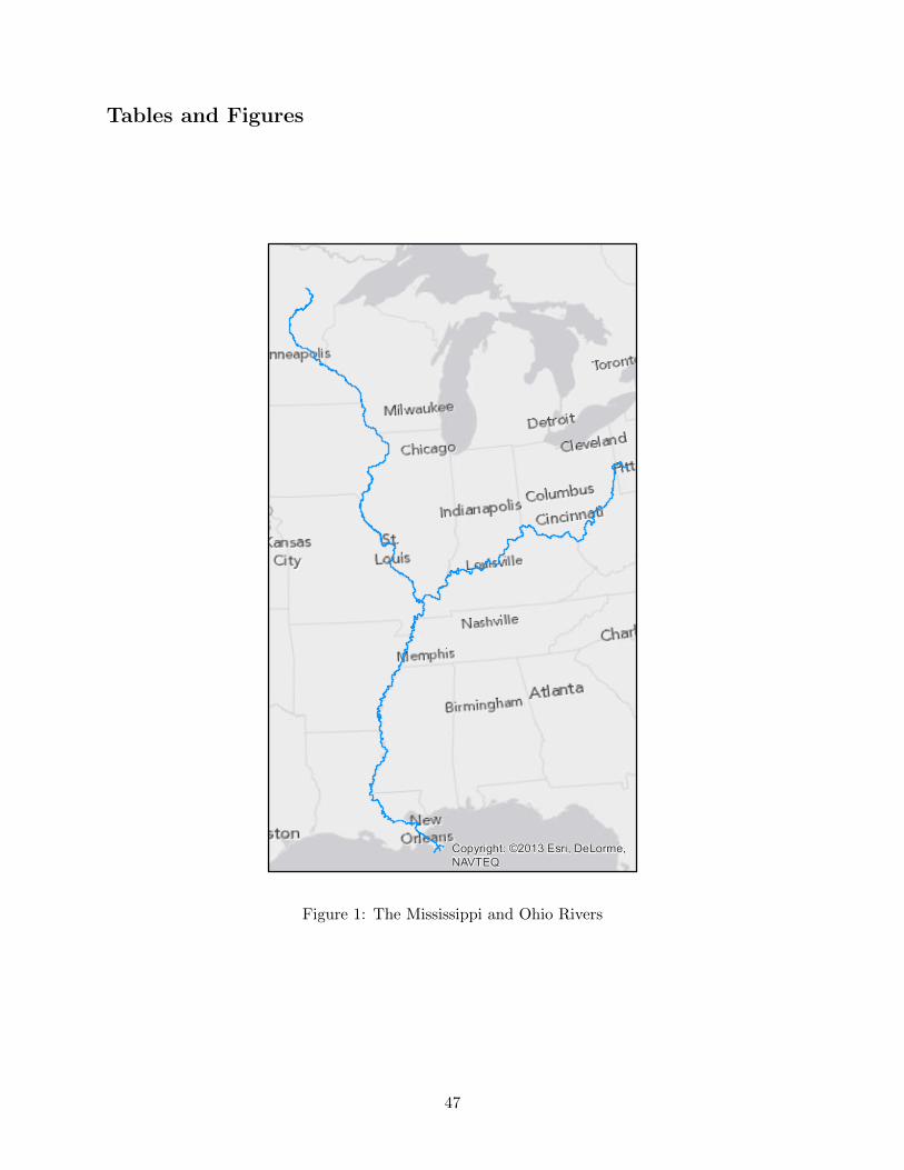
Tables and Figures

Copyright: ©2013 Esri, DeLorme,NAVTEQ

Figure 1: The Mississippi and Ohio Rivers

47

!

!

!

!

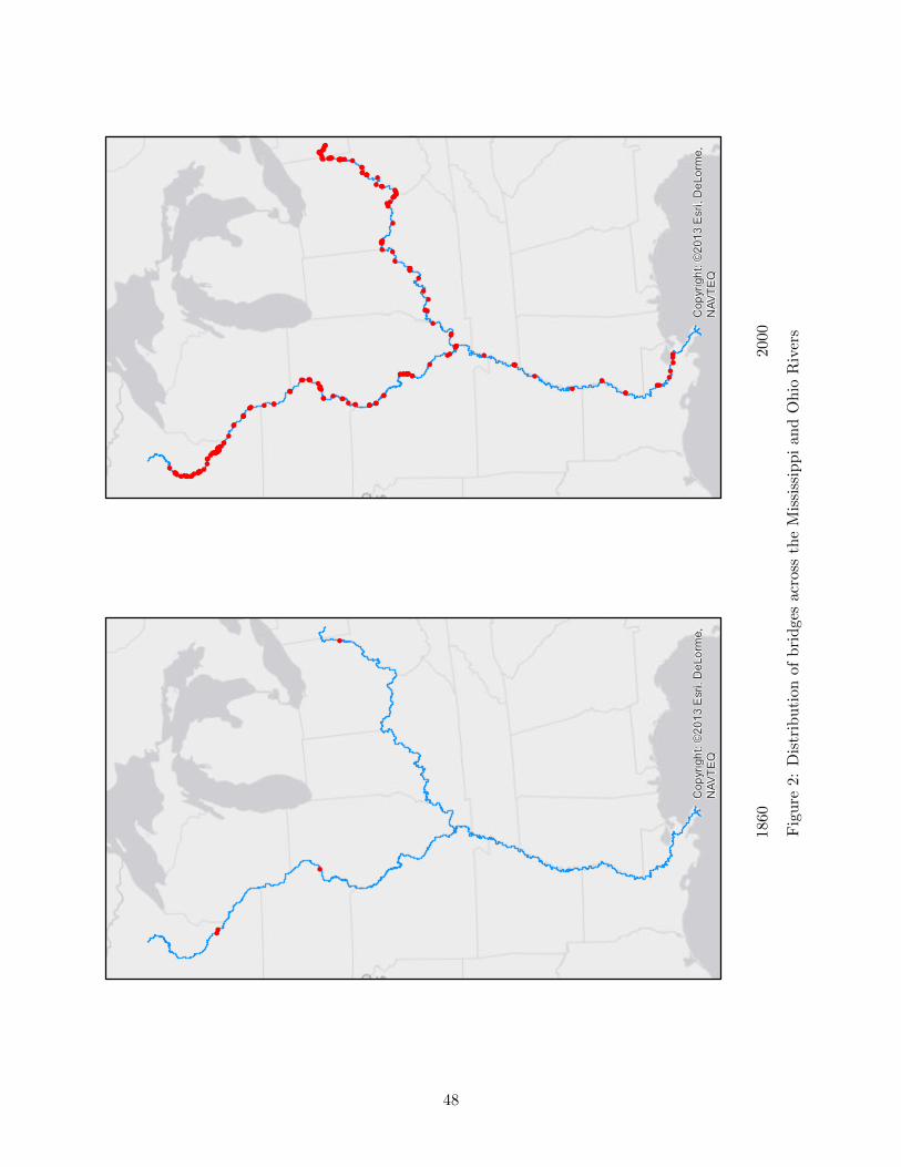
Copy

right:

©20

13 E

sri, D

eLorm

e,NA

VTEQ

1860

!

!

! !!

!

!

!

!

!

!

!

!!

!

!

!

!

!

!

!

!!!

!

!

!

!

!

!!

!

!

!!

!

!

!

! !

!!

!

!

!

!

!

!

!

!

!

!

!

!

!

!

!

!

!!

!!

!

!!

!

!

!

!

!!

!!

!

!

!

!

!

!

!

!

!

!

!!

!

!

!

!

!

!

!

!

!

!

!

!

!

!

!

!

!

!

!!

!

!

!!

!

!

!

!

!

!

!!

!!

!

!!

!

!

!

!

!

!

!

!

!

!

!

!

!

!

!

!

!

!

!

!

!

!!

!

!

!

!

!!

!

!

!

!

!

!

!

!

!

!

!

!

!!!

!

!!

!

!!

!

!

!

!!

!!

!

! !

!

!

!

!

!

! !

!!

!

!!

!

!

!

!

!

!

!

!

!

!

!

!

!!

!

!

! !!

!

!

!

! !

!

!

!

!

!!

!

!

!!

!

!

!!

Copy

right:

©20

13 E

sri, D

eLorm

e,NA

VTEQ

2000

Fig

ure

2:D

istr

ibu

tion

ofb

rid

ges

acro

ssth

eM

issi

ssip

pi

and

Oh

ioR

iver

s

48

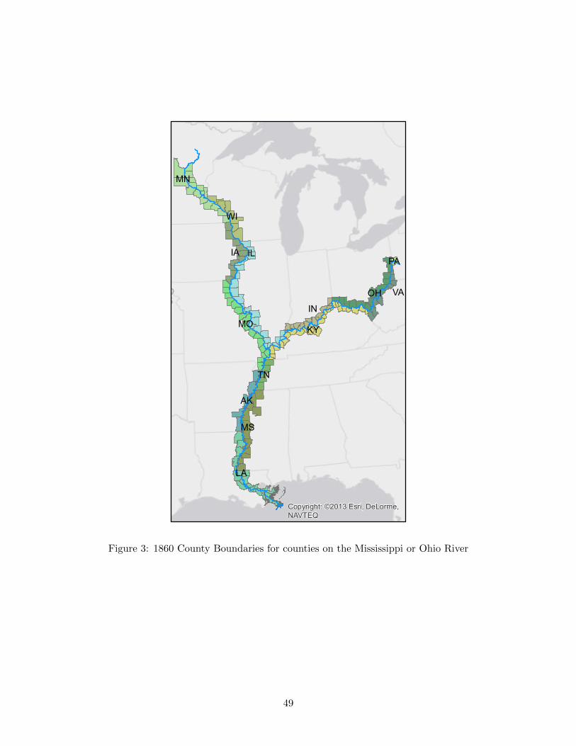
MN

IL

LA

KY

IA

MS

MO

OH

WI

IN

AK

VA

TN

PA

Copyright: ©2013 Esri, DeLorme,NAVTEQ

Figure 3: 1860 County Boundaries for counties on the Mississippi or Ohio River

49

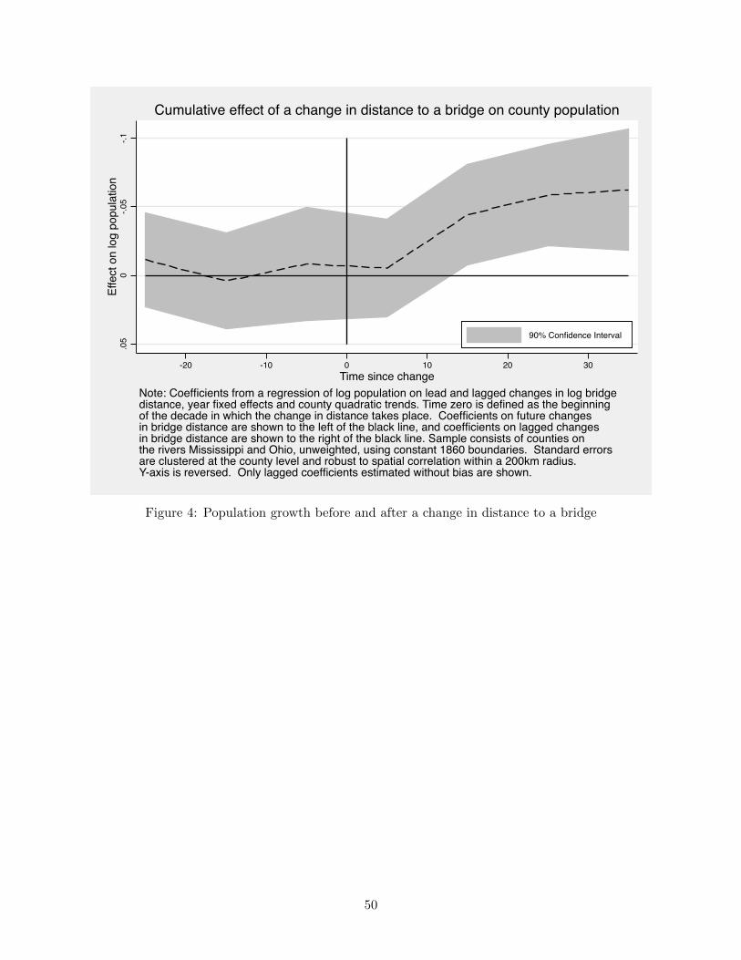
-.1-.0

50

.05

Effe

ct o

n lo

g po

pula

tion

-20 -10 0 10 20 30Time since change

90% Confidence Interval

Note: Coefficients from a regression of log population on lead and lagged changes in log bridgedistance, year fixed effects and county quadratic trends. Time zero is defined as the beginningof the decade in which the change in distance takes place. Coefficients on future changesin bridge distance are shown to the left of the black line, and coefficients on lagged changesin bridge distance are shown to the right of the black line. Sample consists of counties onthe rivers Mississippi and Ohio, unweighted, using constant 1860 boundaries. Standard errorsare clustered at the county level and robust to spatial correlation within a 200km radius.Y-axis is reversed. Only lagged coefficients estimated without bias are shown.

Cumulative effect of a change in distance to a bridge on county population

Figure 4: Population growth before and after a change in distance to a bridge

50

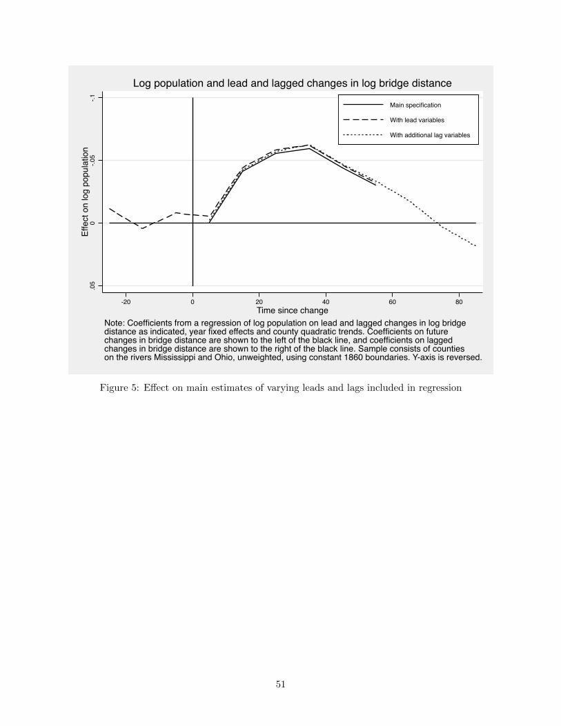
-.1-.0

50

.05

Effe

ct o

n lo

g po

pula

tion

-20 0 20 40 60 80Time since change

Main specification

With lead variables

With additional lag variables

Note: Coefficients from a regression of log population on lead and lagged changes in log bridgedistance as indicated, year fixed effects and county quadratic trends. Coefficients on futurechanges in bridge distance are shown to the left of the black line, and coefficients on laggedchanges in bridge distance are shown to the right of the black line. Sample consists of countieson the rivers Mississippi and Ohio, unweighted, using constant 1860 boundaries. Y-axis is reversed.

Log population and lead and lagged changes in log bridge distance

Figure 5: Effect on main estimates of varying leads and lags included in regression

51

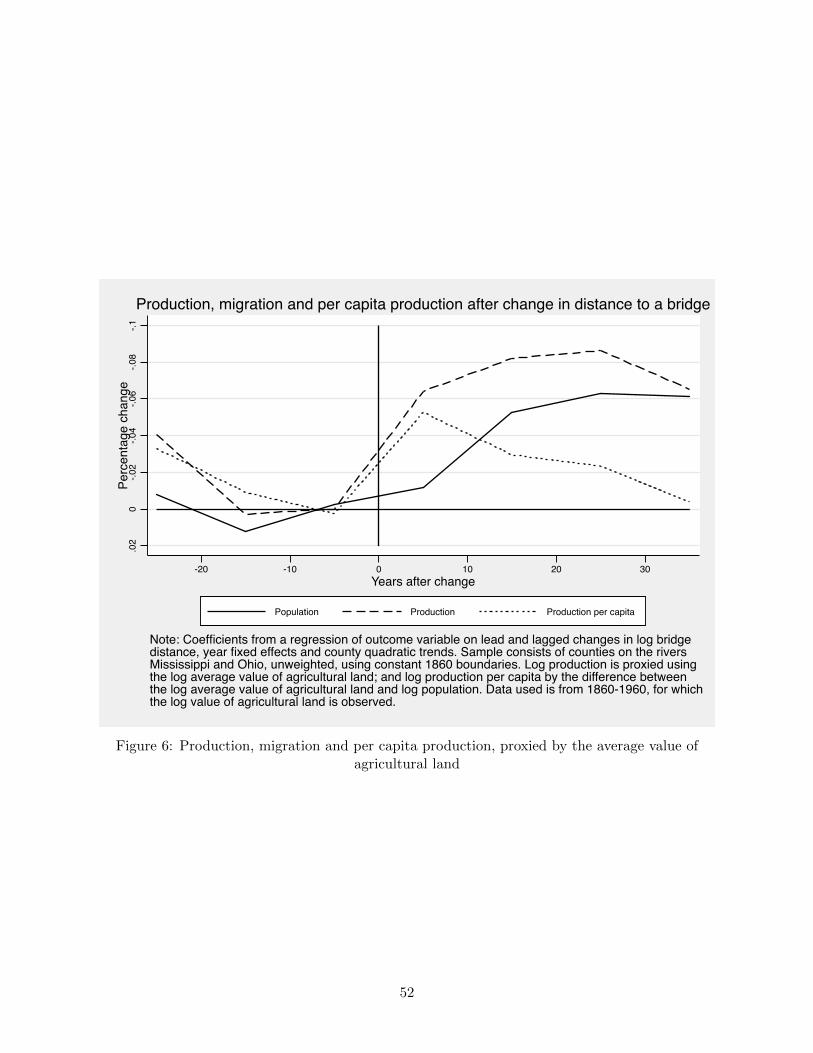
.02

0-.0

2-.0

4-.0

6-.0

8-.1

Perc

enta

ge c

hang

e

-20 -10 0 10 20 30Years after change

Population Production Production per capita

Note: Coefficients from a regression of outcome variable on lead and lagged changes in log bridgedistance, year fixed effects and county quadratic trends. Sample consists of counties on the riversMississippi and Ohio, unweighted, using constant 1860 boundaries. Log production is proxied usingthe log average value of agricultural land; and log production per capita by the difference betweenthe log average value of agricultural land and log population. Data used is from 1860-1960, for whichthe log value of agricultural land is observed.

Production, migration and per capita production after change in distance to a bridge

Figure 6: Production, migration and per capita production, proxied by the average value ofagricultural land

52

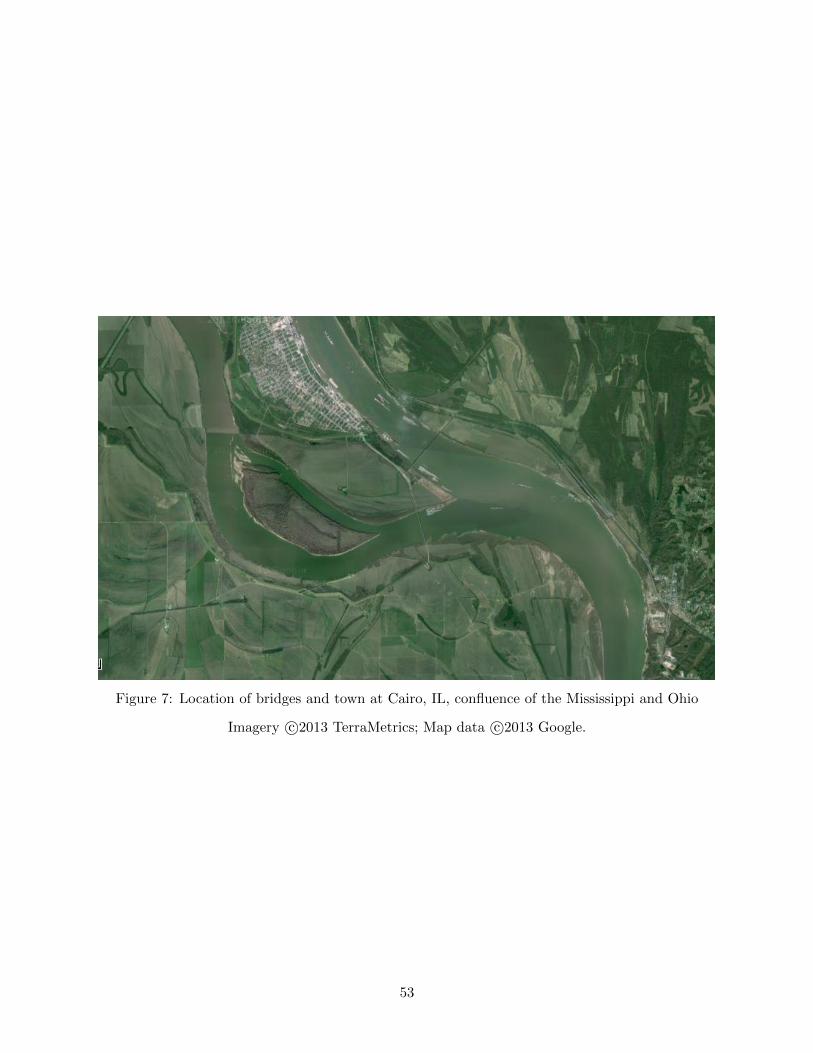
Figure 7: Location of bridges and town at Cairo, IL, confluence of the Mississippi and Ohio

Imagery c©2013 TerraMetrics; Map data c©2013 Google.

53

-.2-.1

0.1

.2Lo

g flo

w ra

te

-50 -25 0 25 50Distance from tributary (km)

a) Flow rate

-.6-.3

0.3

.6Pr

obab

ility

of b

ridge

pre

senc

e

-50 -25 0 25 50Distance from tributary (km)

b) Bridges-.8

-.40

.4.8

Log

dist

ance

from

a b

ridge

-50 -25 0 25 50Distance from tributary (km)

c) Distance from a bridge

-1-.5

0.5

1Lo

g po

pula

tion

dens

ity

-50 -25 0 25 50Distance from tributary (km)

d) Population density

-.4-.2

0.2

.4Lo

g pe

r cap

ita in

com

e

-50 -25 0 25 50Distance from tributary (km)

e) Per-capita income

-.8-.4

0.4

.8Lo

g to

tal e

arni

ngs

/ km

2

-50 -25 0 25 50Distance from tributary (km)

f) Earnings density

Graphs show results from a locally weighted regression of the outcome variableon distance from a tributary, for census tracts less than 50km from a tributaryconfluence. Outcome variables were previously demeaned at the nearesttributary level. Upstream tracts and downstream tracts are pooled separately.

Bridges, population and earnings around tributaries (2000)

Upstream Downstream

Figure 8: Variation in bridge location, population density and earnings around tributaries

54

Table 1: Summary Statistics: Bridges

Numberbuilt

Rail Max spanlength

Total length Daily traffic

(m) (m) c. 2005

Pre-1860 4 0.25 174 415 119501860-1880 29 0.83 111 843 138991880-1900 49 0.51 121 766 198701900-1920 27 0.44 141 1061 97441920-1940 40 0.08 189 935 132211940-1960 20 0.05 221 1053 287571960-1980 42 0.00 190 975 504001980-2000 18 0.00 225 762 20865

All 229 0.28 169 923 26105

Note: Data on bridges covers range of counties described in text. Bridges included are those whichintersect the county sample. Traffic counts are from 2001-2006 and 33 road bridges have missingdata. I dropped traffic data from one bridge where the count was from 1993, and from a rail bridgewhich appeared to have road traffic data listed in error.

Table 2: Summary Statistics: Bridge access by county

Counties withbridges

No. of bridgesever built

No. of extantbridges

Distance to bridge (km)

Bridges? Ever Ever Ever Ever Never

1860 0.06 0.06 0.06 354 5921880 0.36 0.52 0.52 162 3061900 0.56 1.25 1.25 82 1431920 0.60 1.67 1.67 78 1401940 0.73 2.26 2.23 25 461960 0.85 2.57 2.48 23 441980 0.96 3.21 2.94 18 382000 0.98 3.49 3.09 17 38

Note: All counties are on the Missisppi or Ohio Rivers. Counties included in the sample are thosewhich completely overlap the bridge dataset. N = 181 of which: 124 counties ever acquire bridges;57 counties never acquire bridges.

55

Table 3: Summary Statistics: County population

Population PopulationDensity

Annualaveragegrowth

Relativevariance in logpop. density/km2

Panel A: All counties (N = 181)1860 16866 16 0.741880 25921 24 2.5% 0.461900 35459 33 1.3% 0.441920 43126 40 0.3% 0.541940 52618 49 0.5% 0.641960 67642 64 0.4% 0.831980 77766 73 0.7% 0.922000 83604 78 0.2% 1.00

Panel B: Counties acquiring bridges (N = 124)1860 19686 19 0.931880 30773 29 2.7% 0.541900 43023 41 1.4% 0.521920 53801 52 0.5% 0.651940 66754 65 0.6% 0.761960 88532 85 0.7% 0.951980 101197 97 0.8% 0.982000 107888 103 0.2% 1.05

Panel C: Counties never acquiring bridges (N = 57)1860 10731 9 0.271880 15366 13 2.0% 0.181900 19004 15 1.0% 0.141920 19902 15 -0.1% 0.131940 21864 16 0.3% 0.141960 22198 16 -0.2% 0.211980 26795 20 0.4% 0.342000 30776 23 0.2% 0.45

Note: Counties included in the sample are those on the Missisppi or Ohio Rivers which completelyoverlap the bridge dataset. Growth refers to the average annual growth in the preceding twentyyears, approximated by taking the log difference and dividing by 20. Relative variance in logpopulation density is calculated by taking logs of population density, calculating the variance for agiven time and dividing by the same measure calculated for the full sample in the year 2000.

56

Table 4: Probability of bridge construction and location characteristics

Outcome variable: Indicator for construction of a new bridge(1) (2) (3) (4) (5)

Already hasbridge?

Coefficient 0.143*** 0.159*** -0.047 -0.124*** -0.379***s.e. 0.021 0.025 0.032 0.046 0.055

Year FE No Yes Yes Yes YesCounty FE No No Yes Yes Yes

County-specific time trends No No No Linear Quadratic

Note: Coefficients from regressions of an indicator for new bridge construction in a county on anindicator for whether or not the county has a pre-existing bridge and year and county fixed effectsand county-specific time trends as specified in the table. Sample consists of counties on the riversMississippi and Ohio, unweighted, using constant 1860 boundaries. Standard errors clustered bycounty and robust to spatial correlation within 200km. N = 181, T = 18. *** p<0.01, ** p<0.05,* p<0.1.

57

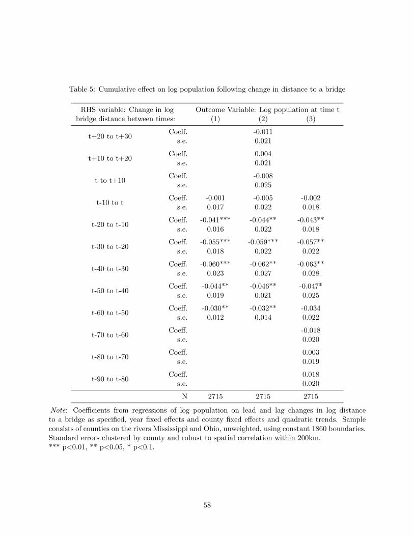
Table 5: Cumulative effect on log population following change in distance to a bridge

RHS variable: Change in logbridge distance between times:

Outcome Variable: Log population at time t(1) (2) (3)

t+20 to t+30Coeff. -0.011

s.e. 0.021

t+10 to t+20Coeff. 0.004

s.e. 0.021

t to t+10Coeff. -0.008

s.e. 0.025

t-10 to tCoeff. -0.001 -0.005 -0.002

s.e. 0.017 0.022 0.018

t-20 to t-10Coeff. -0.041*** -0.044** -0.043**

s.e. 0.016 0.022 0.018

t-30 to t-20Coeff. -0.055*** -0.059*** -0.057**

s.e. 0.018 0.022 0.022

t-40 to t-30Coeff. -0.060*** -0.062** -0.063**

s.e. 0.023 0.027 0.028

t-50 to t-40Coeff. -0.044** -0.046** -0.047*

s.e. 0.019 0.021 0.025

t-60 to t-50Coeff. -0.030** -0.032** -0.034

s.e. 0.012 0.014 0.022

t-70 to t-60Coeff. -0.018

s.e. 0.020

t-80 to t-70Coeff. 0.003

s.e. 0.019

t-90 to t-80Coeff. 0.018

s.e. 0.020

N 2715 2715 2715

Note: Coefficients from regressions of log population on lead and lag changes in log distanceto a bridge as specified, year fixed effects and county fixed effects and quadratic trends. Sampleconsists of counties on the rivers Mississippi and Ohio, unweighted, using constant 1860 boundaries.Standard errors clustered by county and robust to spatial correlation within 200km.*** p<0.01, ** p<0.05, * p<0.1.

58

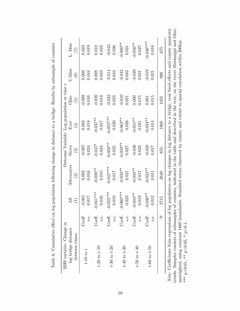
Tab

le6:

Cu

mu

lati

veeff

ect

onlo

gp

opu

lati

onfo

llow

ing

chan

gein

dis

tan

ceto

ab

rid

ge:

Res

ult

sby

sub

sam

ple

ofco

unti

es

RH

Sva

riab

le:

Ch

an

gein

log

bri

dge

dis

tance

bet

wee

nti

mes

:

Ou

tcom

eV

aria

ble

:L

ogp

opu

lati

onat

tim

et

All

Alt

ern

ativ

eN

ever

Eve

rO

hio

U.M

iss

L.

Mis

s(1

)(2

)(3

)(4

)(5

)(6

)(7

)

t-10

tot

Coeff

.-0

.001

0.00

2-0

.007

0.00

3-0

.008

0.00

90.

023

s.e.

0.01

70.

016

0.02

40.

018

0.01

60.

044

0.01

9

t-20

tot-

10C

oeff

.-0

.041*

**-0

.038

**-0

.047

*-0

.037

**-0

.020

0.00

80.

010

s.e.

0.01

60.

015

0.02

40.

017

0.01

90.

043

0.02

5

t-30

tot-

20C

oeff

.-0

.055*

**-0

.047

***

-0.0

58**

-0.0

55**

*-0

.022

-0.0

14-0

.043

s.e.

0.01

80.

017

0.02

50.

020

0.02

30.

043

0.03

0

t-40

tot-

30C

oeff

.-0

.060*

**-0

.050

**-0

.059

**-0

.063

**-0

.010

-0.0

42-0

.080

**s.

e.0.

023

0.02

10.

027

0.02

60.

021

0.04

30.

031

t-50

tot-

40C

oeff

.-0

.044

**-0

.034

**-0

.036

-0.0

51**

0.00

0-0

.029

-0.0

56**

s.e.

0.01

90.

017

0.02

30.

021

0.01

50.

031

0.02

7

t-60

tot-

50C

oeff

.-0

.030

**-0

.024

**-0

.028

-0.0

34**

0.00

1-0

.019

-0.0

46**

*s.

e.0.

012

0.01

10.

017

0.01

40.

015

0.02

10.

016

N27

1526

4085

518

6010

3599

067

5

Note

:C

oeffi

cien

tsfr

om

regr

essi

ons

of

log

pop

ula

tion

onla

gch

ange

sin

log

dis

tan

ceto

ab

rid

ge,

year

fixed

effec

tsan

dco

unty

qu

adra

tic

tren

ds.

Sam

ple

sco

nsi

sts

ofsu

bsa

mp

les

ofco

unti

es,

ind

icat

edin

the

tab

lean

dd

escr

ibed

inth

ete

xt,

onth

eri

vers

Mis

siss

ipp

ian

dO

hio

,u

nw

eigh

ted

,u

sin

gco

nst

ant

1860

bou

nd

arie

s.S

tan

dar

der

rors

clu

ster

edby

cou

nty

and

rob

ust

tosp

atia

lco

rrel

atio

nw

ith

in20

0km

.***

p<

0.01

,**

p<

0.05

,*

p<

0.1

.

59

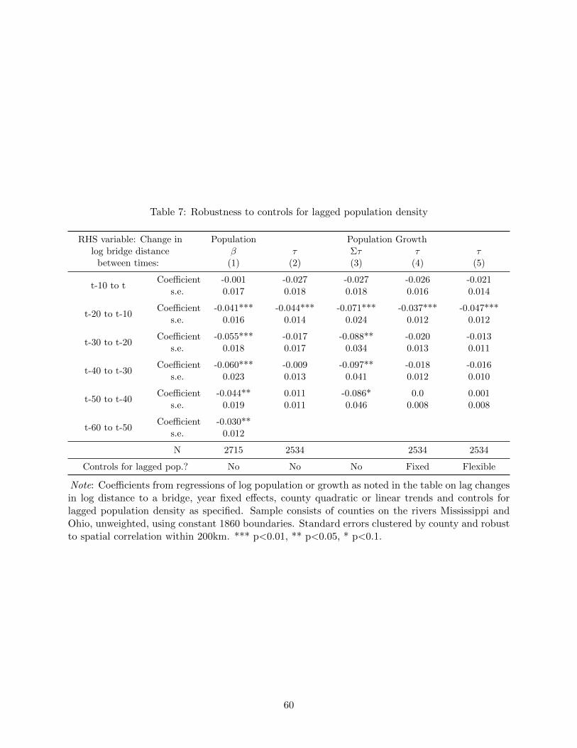
Table 7: Robustness to controls for lagged population density

RHS variable: Change inlog bridge distance

between times:

Population Population Growthβ τ Στ τ τ

(1) (2) (3) (4) (5)

t-10 to tCoefficient -0.001 -0.027 -0.027 -0.026 -0.021

s.e. 0.017 0.018 0.018 0.016 0.014

t-20 to t-10Coefficient -0.041*** -0.044*** -0.071*** -0.037*** -0.047***

s.e. 0.016 0.014 0.024 0.012 0.012

t-30 to t-20Coefficient -0.055*** -0.017 -0.088** -0.020 -0.013

s.e. 0.018 0.017 0.034 0.013 0.011

t-40 to t-30Coefficient -0.060*** -0.009 -0.097** -0.018 -0.016

s.e. 0.023 0.013 0.041 0.012 0.010

t-50 to t-40Coefficient -0.044** 0.011 -0.086* 0.0 0.001

s.e. 0.019 0.011 0.046 0.008 0.008

t-60 to t-50Coefficient -0.030**

s.e. 0.012

N 2715 2534 2534 2534

Controls for lagged pop.? No No No Fixed Flexible

Note: Coefficients from regressions of log population or growth as noted in the table on lag changesin log distance to a bridge, year fixed effects, county quadratic or linear trends and controls forlagged population density as specified. Sample consists of counties on the rivers Mississippi andOhio, unweighted, using constant 1860 boundaries. Standard errors clustered by county and robustto spatial correlation within 200km. *** p<0.01, ** p<0.05, * p<0.1.

60

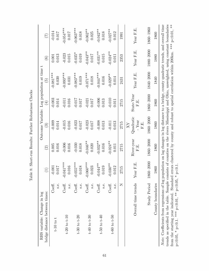
Tab

le8:

Sh

ort-

run

Res

ult

s:F

urt

her

Rob

ust

nes

sC

hec

ks

RH

Sva

riab

le:

Ch

ange

inlo

gb

rid

ged

ista

nce

bet

wee

nti

mes

:O

utc

ome

Var

iab

le:

Log

pop

ula

tion

atti

me

t(1

)(2

)(3

)(4

)(5

)(6

)(7

)

t-10

tot

Coeff

.-0

.001

0.00

5-0

.009

-0.0

03-0

.081*

**

0.0

01

-0.0

14

s.e.

0.01

70.

016

0.01

40.

014

0.0

30

0.013

0.0

17

t-20

tot-

10C

oeff

.-0

.041

***

-0.0

06-0

.015

-0.0

11-0

.093*

**

-0.0

23

-0.0

54***

s.e.

0.01

60.

016

0.01

60.

016

0.0

31

0.015

0.0

17

t-30

tot-

20C

oeff

.-0

.055

***

-0.0

30-0

.023

-0.0

17-0

.083*

**

-0.0

35*

-0.0

63***

s.e.

0.01

80.

018

0.01

70.

017

0.0

19

0.019

0.0

18

t-40

tot-

30C

oeff

.-0

.060

***

-0.0

46**

-0.0

23-0

.021

-0.0

71*

**

-0.0

43**

-0.0

62**

s.e.

0.02

30.

020

0.01

70.

017

0.0

18

0.017

0.0

25

t-50

tot-

40C

oeff

.-0

.044

**-0

.032

**-0

.008

-0.0

06-0

.044***

-0.0

31**

-0.0

42**

s.e.

0.01

90.

016

0.01

30.

013

0.0

16

0.015

0.0

18

t-60

tot-

50C

oeff

.-0

.030

**-0

.024

**-0

.011

-0.0

10-0

.029*

*-0

.024

**

-0.0

27**

s.e.

0.01

20.

011

0.01

30.

011

0.0

14

0.011

0.0

12

N27

1527

1527

1527

15243

1235

3199

1

Ove

rall

tim

etr

end

sY

ear

F.E

.R

iver

-yea

rF

.E.

XY

Qu

adra

tic

-Y

ear

F.E

.

Sta

te-Y

ear

F.E

.Y

ear

F.E

.Y

ear

F.E

.Y

ear

F.E

.

Stu

dy

Per

iod

1860

–200

018

60–2

000

1860

–200

018

60–2

000

1840–2

000

1880–

2000

1860–

1960

Cou

nty

bou

nd

arie

s18

6018

6018

6018

601840

1880

1860

Note

:C

oeffi

cien

tsfr

omre

gre

ssio

ns

oflo

gp

opu

lati

onon

lag

chan

ges

inlo

gd

ista

nce

toa

bri

dge

,co

unty

qu

adra

tic

tren

ds,

and

over

all

tim

etr

end

sas

spec

ified

inth

eta

ble

.S

amp

leco

nsi

sts

ofco

unti

eson

the

rive

rsM

issi

ssip

pi

and

Oh

io,

unw

eigh

ted

,u

sin

gco

nst

ant

bou

nd

arie

sfr

om

the

star

tin

gye

arin

dic

ate

d.

Sta

nd

ard

erro

rscl

ust

ered

by

cou

nty

and

rob

ust

tosp

atia

lco

rrel

atio

nw

ith

in20

0km

.**

*p<

0.01

,**

p<

0.05

,*

p<

0.1.

***

p<

0.0

1,**

p<

0.0

5,*

p<

0.1.

61

Tab

le9:

Sh

ort-

run

Res

ult

s:H

eter

ogen

eity

ofIm

pac

ts

RH

Sva

riab

le:

Ch

ange

inlo

gbri

dge

dis

tan

ceb

etw

een

tim

es:

Ou

tcom

eV

ari

able

:L

ogp

opu

lati

onat

tim

et

Fra

c.U

rb.

Fra

c.W

ork

forc

ein

Ag.

All

For

eign

bor

nN

ativ

eb

orn

Roa

dR

ail

Ear

lyL

ate

(1)

(2)

(3)

(4)

(5)

(6)

(7)

(8)

(9)

t-10

tot

Coeff

.-0

.001

-0.0

93*

0.0

0.01

1-0

.026

-0.0

04-0

.002

-0.0

02

0.015

s.e.

0.01

70.

055

0.0

17

0.0

17

0.02

00.

024

0.01

80.0

060.

013

t-20

tot-

10C

oeff

.-0

.041

***

-0.1

81**

*-0

.045

***

-0.0

24-0

.035*

-0.0

48**

-0.0

30-0

.011*

0.027*

s.e.

0.01

60.

062

0.0

17

0.0

15

0.02

10.

020

0.02

10.0

060.

014

t-30

tot-

20C

oeff

.-0

.055

***

-0.1

68**

*-0

.059

***

-0.0

39*

*-0

.054*

*-0

.056

***

-0.0

60**

-0.0

14**

0.0

16s.

e.0.

018

0.05

80.0

19

0.0

17

0.02

60.

021

0.02

50.0

060.

011

t-40

tot-

30C

oeff

.-0

.060

***

-0.1

49**

*-0

.050

**-0

.048*

*-0

.044*

-0.0

57*

-0.0

70*

**-0

.015

***

0.0

27*

*s.

e.0.

023

0.05

20.0

22

0.0

23

0.02

60.

031

0.02

60.0

050.

012

t-50

tot-

40C

oeff

.-0

.044

**-0

.052

-0.0

39**

-0.0

27-0

.032

*-0

.045

-0.0

44**

-0.0

08*

0.0

11

s.e.

0.01

90.

052

0.0

19

0.0

20

0.01

90.

029

0.01

80.0

040.

007

t-60

tot-

50C

oeff

.-0

.030

**-0

.038

-0.0

26**

-0.0

13-0

.032

**-0

.026

-0.0

39*

**-0

.003

s.e.

0.01

20.

042

0.0

12

0.0

12

0.01

30.

020

0.01

10.0

03

N27

1518

1020

38

2715

271

527

15

2715

2351

140

9

Note

:C

oeffi

cien

tsfr

om

regr

essi

ons

of

log

pop

ula

tion

onla

gch

ange

sin

log

dis

tan

ceto

ab

rid

ge,

year

fixed

effec

tsan

dco

unty

qu

adra

tic

tren

ds,

exce

pt

inco

lum

ns

4)

and

5)w

her

eth

eR

HS

vari

able

sar

ela

gged

chan

ges

inlo

gd

ista

nce

toa

road

and

rail

bri

dge

,re

spec

tive

ly.

Res

ult

sin

colu

mn

s6)

an

d7)

from

are

gre

ssio

nof

log

pop

ula

tion

onla

gch

ange

sin

log

dis

tan

ceto

ab

rid

gean

dth

esa

me

contr

ols,

wh

ere

the

lagg

edd

ista

nce

vari

ab

les

are

inte

ract

edw

ith

anin

dic

ator

for

wh

eth

erth

eob

serv

atio

nis

inth

efi

rst

orse

con

dh

alf

ofth

eti

me

per

iod

stu

die

d.

Sam

ple

sco

nsi

sts

of

sub

sam

ple

sof

cou

nti

es,

ind

icat

edin

the

tab

lean

dd

escr

ibed

inth

ete

xt,

onth

eri

ver

sM

issi

ssip

pi

and

Oh

io,

unw

eigh

ted

,u

sin

gco

nst

ant

1860

bou

nd

arie

s.S

tan

dar

der

rors

clu

ster

edby

cou

nty

and

rob

ust

tosp

atia

lco

rrel

atio

nw

ith

in20

0km

.**

*p<

0.01

,**

p<

0.05

,*

p<

0.1

.

62

Table 10: Cumulative effect on log population, log average value of agricultural land, anddifference

RHS variable: Change in logbridge distance between times:

Logpopulation

Log valueag. land

Difference

(1) (2) (3)

t-10 to tCoeff. -0.012 -0.062** -0.050*

s.e. 0.017 0.029 0.028

t-20 to t-10Coeff. -0.054*** -0.083** -0.030

s.e. 0.016 0.040 0.038

t-30 to t-20Coeff. -0.063*** -0.088** -0.025

s.e. 0.018 0.039 0.041

t-40 to t-30Coeff. -0.062** -0.066* -0.005

s.e. 0.025 0.038 0.034

t-50 to t-40Coeff. -0.042** 0.001 0.043

s.e. 0.018 0.028 0.029

t-60 to t-50Coeff. -0.026** 0.005 0.031

s.e. 0.012 0.027 0.028

N 1986 1986 1986

Note: Coefficients from regressions of outcome variables on on lagged changes in log distance to abridge, year fixed effects and county fixed effects and quadratic trends. Sample consists of countieson the rivers Mississippi and Ohio, unweighted, using constant 1860 boundaries, for decadal intervalsbetween 1860 and 1960, consistent with the availability of the land values data. Standard errorsclustered by county and robust to spatial correlation within 200km.*** p<0.01, ** p<0.05, * p<0.1.

63

Tab

le11:

Lon

g-ru

nR

esu

lts:

Cro

ss-s

ecti

onal

rela

tion

ship

(200

0)

Log

pop

ula

tion

den

sity

Log

per

-capit

ain

com

eL

ogea

rnin

gd

ensi

ty(1

)(2

)(3

)(4

)(5

)(6

)(7

)

Log

bri

dge

dis

tance

Coeff

.-0

.69*

**-0

.67*

**-0

.31*

**-0

.03

0.05

***

-0.7

0***

-0.2

6***

s.e.

0.07

0.12

0.08

0.02

0.01

0.13

0.08

N241

712

8512

8512

8412

8412

8412

84

Con

trol

sN

oN

oY

esN

oY

esN

oY

esT

rib

uta

ryF

.E.

No

No

Yes

No

Yes

No

Yes

Sam

ple

All

50km

50km

50km

50km

50km

1840

Note

:C

oeffi

cien

tsfr

omO

LS

regr

essi

ons

of

outc

ome

vari

able

list

edon

log

dis

tan

ceto

ab

rid

gein

the

year

2000

.C

ontr

ols

com

pri

sea

qu

adra

tic

fun

ctio

nof

dis

tan

ceto

the

nea

rest

trib

uta

ry,

and

pat

hle

ngt

hfr

omth

eri

ver

mou

thin

tera

cted

wit

hri

ver

indic

ator

s.S

amp

leco

nsi

sts

of2000

cen

sus

tract

sw

her

eany

par

tof

the

trac

tis

wit

hin

10km

ofth

eM

issi

ssip

pi

orO

hio

rive

rs.

Sta

nd

ard

erro

rsar

ecl

ust

ered

by

nea

rest

trib

uta

ryan

du

pst

ream

stat

us

(Nc

=56

for

sam

ple

wit

hin

50km

oftr

ibu

tari

es.)

.**

*p<

0.01

,**

p<

0.05

,*

p<

0.1.

64

Tab

le12

:L

ong-

run

Res

ult

s:F

irst

stag

ean

dre

du

ced

form

Log

bri

dge

dis

t.(2

000)

Log

pop

.d

ens.

(200

0)

Log

pop

.d

ens.

(200

0)

Log

pop

.d

ens.

(184

0)

Log

p.c

.in

c.(2

000)

Log

earn

.d

ens.

(200

0)(1

)(2

)(3

)(4

)(5

)(6

)

Up

stre

amC

oeff

.-1

.21*

**0.

62*

0.96

0.02

-0.2

1**

0.42

s.e.

0.29

0.37

0.58

0.12

0.10

0.32

Up

stre

amx

dis

tan

cefr

om

trib

uta

ryC

oeff

.0.

14**

*-0

.03

-0.0

8-0

.03

0.03

**-0

.01

s.e.

0.03

0.03

0.06

0.02

0.01

0.03

Up

stre

amx

dis

tan

cefr

om

trib

uta

ry2

Coeff

.-0

.002

8***

0.00

040.

0012

0.00

04-0

.000

6*-0

.000

2s.

e.0.

0008

0.00

060.

0011

0.00

040.

0003

0.00

06

N12

8712

8574

674

712

8412

84

Sam

ple

50km

50km

1840

1840

50km

50km

Note

:C

oeffi

cien

tsfr

omO

LS

regre

ssio

ns

ofou

tcom

eva

riab

leli

sted

onva

riab

les

list

edin

the

year

tab

le,

nea

rest

trib

uta

ryfixed

effec

tsan

dgeo

gra

ph

icco

ntr

ols

com

pri

sin

ga

qu

ad

rati

cfu

nct

ion

ofd

ista

nce

toth

en

eare

sttr

ibu

tary

,an

dp

ath

len

gth

from

the

river

mou

thin

tera

cted

wit

hri

ver

ind

icat

ors

.S

amp

leco

nsi

sts

of200

0ce

nsu

str

acts

wh

ere

any

par

tof

the

trac

tis

wit

hin

10km

ofth

eM

issi

ssip

pi

orO

hio

river

s.S

tan

dard

erro

rsare

clu

ster

edby

nea

rest

trib

uta

ryan

du

pst

ream

stat

us

(Nc

=56

for

sam

ple

wit

hin

50km

oftr

ibu

tari

es.)

.**

*p<

0.01

,**

p<

0.0

5,

*p<

0.1

.

65

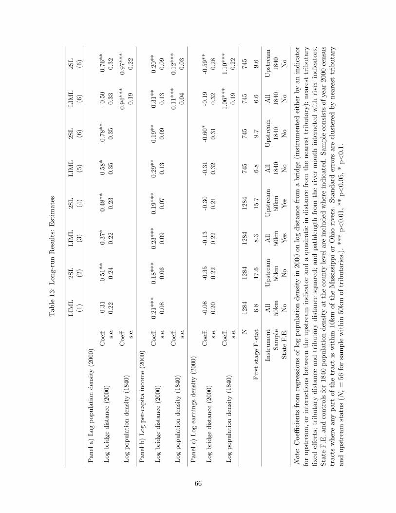
Tab

le13

:L

ong-

run

Res

ult

s:E

stim

ates

LIM

L2S

LL

IML

2SL

LIM

L2SL

LIM

L2SL

(1)

(2)

(3)

(4)

(5)

(6)

(6)

(6)

Pan

ela)

Log

pop

ula

tion

den

sity

(200

0)

Log

bri

dge

dis

tance

(200

0)C

oeff

.-0

.31

-0.5

1**

-0.3

7*

-0.4

8**

-0.5

8*-0

.78**

-0.5

0-0

.76*

*s.

e.0.

22

0.24

0.2

20.

23

0.3

50.

35

0.33

0.3

2

Log

pop

ula

tion

den

sity

(184

0)C

oeff

.0.

94***

0.9

7***

s.e.

0.19

0.22

Pan

elb)

Log

per

-cap

ita

inco

me

(200

0)

Log

bri

dge

dis

tance

(200

0)C

oeff

.0.

21*

**

0.18

***

0.2

3***

0.19*

**

0.29*

*0.1

9**

0.3

1**

0.20

**

s.e.

0.08

0.06

0.0

90.

07

0.1

30.

09

0.13

0.0

9

Log

pop

ula

tion

den

sity

(184

0)C

oeff

.0.

11***

0.1

2***

s.e.

0.04

0.03

Pan

elc)

Log

earn

ings

den

sity

(200

0)

Log

bri

dge

dis

tance

(200

0)C

oeff

.-0

.08

-0.3

5-0

.13

-0.3

0-0

.31

-0.6

0*

-0.1

9-0

.59**

s.e.

0.20

0.22

0.2

20.

21

0.3

20.

31

0.32

0.2

8

Log

pop

ula

tion

den

sity

(184

0)C

oeff

.1.

06***

1.1

0***

s.e.

0.19

0.22

N128

412

84

1284

128

474

5745

745

745

Fir

stst

age

F-s

tat

6.8

17.6

8.3

15.7

6.8

9.7

6.6

9.6

Inst

rum

ent

All

Upst

ream

All

Upst

ream

All

Upst

ream

All

Upst

ream

Sam

ple

50k

m50k

m50

km

50km

184

01840

184

018

40

Sta

teF

.E.

No

No

Yes

Yes

No

No

No

No

Note

:C

oeffi

cien

tsfr

omre

gres

sion

sof

log

pop

ula

tion

den

sity

in20

00on

log

dis

tan

cefr

oma

bri

dge

(in

stru

men

ted

eith

erby

anin

dic

ator

for

up

stre

am

,or

inte

ract

ions

bet

wee

nth

eu

pst

ream

ind

icat

oran

da

qu

adra

tic

ind

ista

nce

from

the

nea

rest

trib

uta

ry);

nea

rest

trib

uta

ryfi

xed

effec

ts;

trib

uta

ryd

ista

nce

and

trib

uta

ryd

ista

nce

squ

ared

;an

dp

ath

len

gth

from

the

rive

rm

outh

inte

ract

edw

ith

rive

rin

dic

ator

s.S

tate

F.E

.an

dco

ntr

ols

for

1840

pop

ula

tion

den

sity

atth

eco

unty

level

are

incl

ud

edw

her

ein

dic

ated

.S

amp

leco

nsi

sts

ofye

ar20

00ce

nsu

str

act

sw

her

ean

yp

art

of

the

tract

isw

ith

in10

km

ofth

eM

issi

ssip

pi

orO

hio

rive

rs.

Sta

nd

ard

erro

rsar

ecl

ust

ered

by

nea

rest

trib

uta

ryan

du

pst

ream

statu

s(N

c=

56fo

rsa

mp

lew

ith

in50

km

oftr

ibu

tari

es.)

.**

*p<

0.01

,**

p<

0.05

,*

p<

0.1.

66

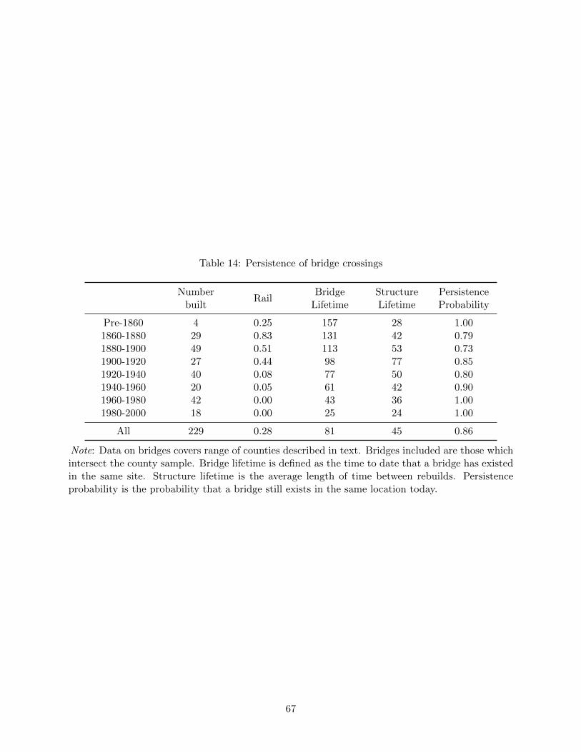
Table 14: Persistence of bridge crossings

Numberbuilt

RailBridge

LifetimeStructureLifetime

PersistenceProbability

Pre-1860 4 0.25 157 28 1.001860-1880 29 0.83 131 42 0.791880-1900 49 0.51 113 53 0.731900-1920 27 0.44 98 77 0.851920-1940 40 0.08 77 50 0.801940-1960 20 0.05 61 42 0.901960-1980 42 0.00 43 36 1.001980-2000 18 0.00 25 24 1.00

All 229 0.28 81 45 0.86

Note: Data on bridges covers range of counties described in text. Bridges included are those whichintersect the county sample. Bridge lifetime is defined as the time to date that a bridge has existedin the same site. Structure lifetime is the average length of time between rebuilds. Persistenceprobability is the probability that a bridge still exists in the same location today.

67

Appendices

Appendix A: Data

Bridge Data

Locational information In the version compiled by the Federal Highway Administration, theNBI normally contains locational information. However, the information is often missing or unveri-fied. The version of the data used was conflated to a common reference network 29 by the Researchand Innovative Technology Administration’s Bureau of Transportation Statistics (RITA/BTS) tocreate a shapefile with locational information where available. However, 25% of locational infor-mation was missing. Information on bridges carrying railways was also missing from the datasetby design (this information is stored in a separate database).

Extract of original sample and initial checking Bridges over the Mississippi or Ohio Riverswere extracted either through string matching (using a text field describing the feature ‘under’ thebridge) or through proximity mapping to river shapefiles using ArcGIS. The dataset of possiblematches was then hand checked using both satellite imagery (accessed through Google Earth) andother contemporary lists of bridges, to ensure completeness with respect to extant bridges. Sincethe NBI is compiled from listings created separately by state and county administrative bodies,bridges that spanned two counties or states were often listed twice. The process of hand checkingalso enabled me to remove duplicate listings of the same bridge.

Supplementary sources of bridge data The data was also cross-checked with alter-native sources of information on bridges, typically compiled by amateur bridge enthusiasts.These alternative sources of information included: (Costello, 1995); (Costello, 2002); and vari-ous websites including: http://bridgehunter.com/; http://www.johnweeks.com/river mississippi/;http://www.bridgemeister.com/; http://bridgestunnels.com/; and Wikipedia. In particular, thealternative sources of information were used to establish the original date of first construction atthe site, since there is a high occurrence of rebuilding of bridge structures, and the date listed inthe NBI often corresponded to the most recent rebuild. Where extant bridges were missing fromthe dataset, I obtained the required information about the bridge from these alternative sources.In a few cases where alternative sources had significantly conflicting or unclear information aboutlocation or number of bridges, I contacted local historical societies to ask them for informationfrom their archives.

Length of maximum span and total length of structure The data on length of maximumspan and total length of structure was either cross-checked with or obtained from the alternativesources listed above. Where data on a structure that still exists was missing from all other sources,I obtained the measurements from satellite images using Google Earth. Where data on a historicalstructure was missing, I obtained the data wherever possible from Office of the Chief of Engineers,United States Army (1948), which lists the width of the navigable channel. This is usually a slightunderestimate of the maximum span, but represented the best available estimate.

Census Data

Mapping bridges to counties The bridge data was spatially mapped to the county data, usingat most a 5000m radius around the coordinates attributed to the bridge. (The bridges are assigneda single point location in the data, but in reality the length of the bridge may be significant).In almost all cases, a bridge treats two counties on either side of the river by connecting them,although there are a few cases, mostly in Louisiana, when both sides of the river are within the

29TeleAtlas’s DynaMap for Transportation

68

same county boundary. Where a bridge is located close to the boundary between two counties, thespatial mapping resulted in more than one or two matches between bridge and county. I cross-checked the original spatial mapping with a spatial mapping with a smaller radius to remove somespurious matches, and hand-checked the remaining matches to ensure that the bridges only matchone county on either side of the river.

Population foreign-born or native-born Aggregate statistics on the proportion of the pop-ulation in a county that is foreign-born are available from the ICPSR dataset for 1870-1900, 1940,1960 and 1990. I estimate the fraction of the county population that is foreign-born using IPUMSdata for all study counties for 1860 and for 1910-1930, and for the subset of counties that coincidewith a PUMA for 1950, 1970, 1980 and 2000. I am therefore able to recover the total foreign bornand native population, and fraction foreign born, for all counties in all years except 1950, 1970,1980 and 2000, for which the information is only available for the largest counties.

Population by race and genderData on the composition of the population by race (black,white and other) and gender is available for all years from the ICPSR dataset, although the defi-nitions used of race are not stable over time.

Urban and rural population Urban population is defined as living in places with 2500 ormore people, following the census convention. The data on urbanization is taken from the ICPSRdatabase, but is only available for the study years up to and including 1980. 23 larger countieshave data available for 1990 using the IPUMS database, but I exclude this data as it is not clearwhether including incomplete years at the end of the sample could affect the results; excluding thedata slightly reduces the magnitude and significance of the results.

Industrial composition of the workforce Data is not consistently available for all sectorsfor the entire time period studied. For the manufacturing sector only, data is available from theICPSR data for the entire time period (with the exception of 1910). For all sectors, I can usehousehold level data from IPUMS to estimate the fraction of the workforce in each industry andrecover the workforce in each industry by multiplying by the population at the time. The IPUMSdata is not available consistently at the county level beyond 1940 and is missing for 1890.

River Data

Datasets The three datasets used to map river data to county data are: 1) Flowlines from theUSGS National Hydrography Dataset (NHD); 2) Environmental Systems Research Institute, Inc(ESRI) US Rivers (Generalized); and 3) Environmental Systems Research Institute, Inc (ESRI) USWaterbodies.

Mapping rivers to counties I code the county as being on one of the rivers if the countyintersects a 200m buffer zone around any of the three river shapefiles, since the shapefiles haveslightly different alignments which may reflect changes in river alignment over time. At the sametime, I record the minimum distance between the county centroid and the river shapefile to obtainthe distance from the county to the river. The river dataset which contains most information aboutriver characteristics is the NHD. To obtain more details about the local characteristics of the river,I assign each reach in the dataset (reaches range between 0.01 and 40 km in length) to the countyon each side of the river with which it shares the greatest overlap by creating a buffer zone aroundthe river. I then use the characteristics of these reaches to calculate local river characteristics e.g.the mean flow across these reaches, the total length of the river that intersects the county.

Instrument construction The river is modelled in the dataset in reaches of a mean length of1.9 km. I first removed river reaches where the data was missing or otherwise clearly misassignede.g. much larger or smaller than the neighbouring reaches. Each reach is assigned a flow rate. Asecond variable describes the incremental increase in the flow rate along the reach. The difference

69

between the flow rate in a downstream segment and the flow rate in the upstream segment plus theincremental addition, is the increase in flow at the junction between the reaches. I define a majortributary as a point at which the increase in flow is greater than 7.5%, or greater than 10,000 cubicfeet per second. For each reach, I then construct a variable that measures the distance in river kmfrom the nearest tributary. I then assign bridges to the nearest river segment; and calculate thedistance between the river segment centroid and the nearest bridge. I then assign census tracts tothe nearest river segment.

70