Breeding Ones’ Own Subprime Crisis

Breeding Ones’ Own Subprime CrisisThe effects of labour market on financial system stability∗

Tomasz Daras

National Bank of Poland

University of Warsaw

Joanna Tyrowicz

University of Warsaw

National Bank of Poland

February, 2009

Abstract

In this paper we take a simulation approach towards household budgets survey, analysing the impact

of changes in labour market status of household members on the ability of this household to service the

mortgage payments.

Using the current status as benchmark, we performed simulations using stylised facts about labour

market evolutions. Households with mortgage are characterised by higher activity rates and lower

unemployment rates than demographically comparable households without a credit. While these are

typical preconditions for the credit approval decision, this state of matters may not necessarily persist

throughout the entire mortgage service period. Firstly, labour market conditions may worsen in general,

comprising the credit takers together with the rest of the population. Alternatively, credit takers may

undergo employment experience in the same way as other labour market participants. Consequently,

we performed analyses along two scenarios: (i) households with mortgages will gradually become alike

the demographically comparable group in terms of employment performance; and (ii) recognising the

fact that debtor households members may exert potentially higher effort in maintaining labour market

status we model the effects of general employment outlooks deterioration. We use labour force survey

data to obtain the probabilities of changing the individual labour market status, while we resort to

propensity score matching techniques to provide adequate benchmark for the changes among creditors

with relation to general population.

In the simulations we find the share of creditors loosing liquidity with the change in the labour

market status and the implied burden to the financial sector stability.

Key words: financial sector stability, mortgages, labour market

JEL Codes: G21, C15, R20

∗Authors would like to thank Michal Gradzewicz, Jacek Laszek, Ryszard Kokoszczynski, Tomaszk Michalak, Kersten Staehr

and Zbigniew Zolkiewski. Usual disclaimer applies.

1 Introduction

In most theoretical approaches, credit worthiness is evaluated basing on ones’ likelihood to maintain thefuture burden of repayments. The origin of riskiness comes from the fact future liquidity of creditorsremains unknown at the time of credit approval. For mortgages, it has been frequently argued in theliterature, that scoring models can help to partly alleviate this problem by allocating potential clientsdifferentiated probability of becoming delinquent in the credit horizon by using the proxies of demographicstatus, educational attainment and subsequently labour market prospects, (Wagner 2004). In principle,these models evaluate the future earnings using a Mincerian approach. On the other hand, in transitioneconomies one observes large swings in the unemployment rate - in the case of Poland the movement from10% to 20% and back to 10% thresholds was observed over less than a decade, which makes it very difficultto evaluate individual future labour market prospects basing on a current employment status.

Consequently, one could pose a research question concerning the risk of observing a crisis similar to sub-prime breakdown in the US as a consequence of deterioration in the Polish labour market. We addressesthis question by developing a simulation framework using individual households’ budgets data for 2007.We observe the liquidity of households burdened with a mortgage loan. We subsequently simulate futureemployment prospects of income earners in these households using adapted labour force survey data.

Naturally, creditors differ from the population at large in terms of labour market situation - theyare more active and definitely more frequently employed. In the simulations, we attempted to comprisetwo competing approaches. The first assumes that credit takers will consistently experience significantlybetter employment prospects due to for example higher search effort. Therefore, their odds of loosing andfinding jobs will evolve together with the market conditions, but starting from the currently observed,significantly higher levels of employment persistence (the likelihood to remain in employment) and find rate(the likelihood of finding new employment). To this end we used LFS data for 1999-2004 period, whichobserved doubling of the general unemployment rate.

In the latter approach, we will not monitor the influence of exogenous labour market shifts that couldoccur for example because of the worsening growth prospects, but focus on endogenous changes in thelabour market performance of the creditors. Namely, the simulated shock will comprise gradually equatingthe probabilities of flows into and out of employment with the comparable demographic groups. Therefore,in the second approach we provide analysis of what would be the effects of continuing with the current,relatively bold labour market conditions if one no longer subscribes to the view that credit takers areinherently different from the comparable non-borrowers in the population in terms of employment prospects.

Our findings suggest that both simulated shocks will noticeably affect the ability of Polish householdsto service the mortgage payments. This impact - depending on the scenario - ranges from 63% to 78%increase in the number of delinquent households, while the volume of endangered credit may reach 3.6% to10.4% of the 2007 outstanding mortgages.

The paper is structured as follows. In section (2) we briefly present the similarities and differencesbetween current situation in Poland and outlooks in the US at the edge of sub-prime crisis emergence.Subsequently we present model setup in section (3). In section (1) we describe the data. Section (5)presents the results and implications for policy.

2 Literature review and context

To the best of our knowledge this type of research is unprecedented in the literature, while this papercontributes in two main ways. First of all, we use propensity score matching for recovered individual datafrom household budgets survey and originally individual data from labour force survey to obtain reliablebenchmark for simulating the suggested scenarios. Secondly, we apply multi-agent systems approach (MAS)using micro-level data to arrive at macroeconomic estimates of financial system stability.

To some extent similar efforts were undertaken by few central banks (including Bank of England, Bank ofCanada and Central Bank of Greece) to use household level data to approximate the distribution of the debt

1

servicing burden, Barwell, Orla and Pezzini (2006), Simigiannis and Tzamourani (2006) and Faraqui (2006).Also for Swedish data this type of scrutiny was undertaken, using the so-called margin approach, whichallows to define the liquidity of households taking into account servicing all debts and covering subsistenceexpenses, (Johansson and Persson 2006). However, both these approaches are backward looking in a sensethat they analyse the indicators already experienced by the economy, while the projections are based onstructural relationships between macro-level aggregates. We take the opposite angle using micro-level datafor simulation exercises obtaining macroeconomic projections as outcome.

For Poland recently, Zajaczkowski and Zochowski (2007) used household budget survey data to performstress-test for monetary and foreign currency shocks, while Osinski, Szpunar and Tymoczko (eds.) (2008)report the results of simulations in case of increased risk of becoming unemployed (unemployment rategrowth by 4.7 percentage point, which is a conservative, ”pessimistic” projection). Both these studies reachthe conclusion that Polish households liquidity is vulnerable to such exogenous shocks, but the stability ofthe financial system should remain unaffected.

Gorton (2008) analyses in detail the origins of the recent financial distress in the US describing how thebanking system crisis emerged in the US from mortgage difficulties in the so-called subprime segment ofcreditors. However, the important conclusion from this text for any other economy experiencing constructionand mortgage booms concerns the very nature of the so called ”subprime” credits. Namely, the terms ”sub-prime” and ”Alt-A” are not official designations of any regulatory authority or rating agency. Basically,the terms refer to borrowers who are perceived to be riskier than the average borrower because of a poorcredit history. Sub-prime or Alt-A credits imply that loan-to-value ratio ranges between 60-70% and100% (better rated mortgages usually do not exceed 80% thresholds). Home ownership for low incomeand minority households has been a long-standing national goal in the U.S. Sub-prime mortgages were aninnovation aimed at meeting this target. The main issue to be confronted in providing mortgage financefor this unserved population was clearly that these borrowers are riskier.

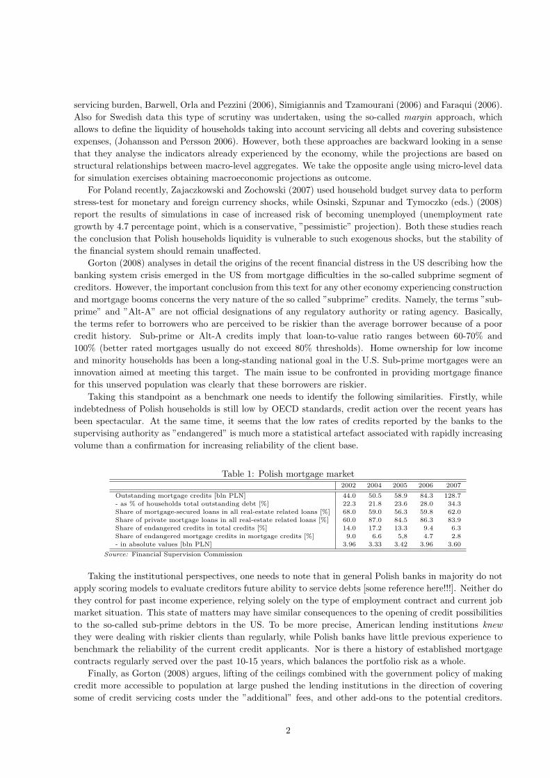
Taking this standpoint as a benchmark one needs to identify the following similarities. Firstly, whileindebtedness of Polish households is still low by OECD standards, credit action over the recent years hasbeen spectacular. At the same time, it seems that the low rates of credits reported by the banks to thesupervising authority as ”endangered” is much more a statistical artefact associated with rapidly increasingvolume than a confirmation for increasing reliability of the client base.

Table 1: Polish mortgage market2002 2004 2005 2006 2007

Outstanding mortgage credits [bln PLN] 44.0 50.5 58.9 84.3 128.7

- as % of households total outstanding debt [%] 22.3 21.8 23.6 28.0 34.3

Share of mortgage-secured loans in all real-estate related loans [%] 68.0 59.0 56.3 59.8 62.0

Share of private mortgage loans in all real-estate related loans [%] 60.0 87.0 84.5 86.3 83.9

Share of endangered credits in total credits [%] 14.0 17.2 13.3 9.4 6.3

Share of endangered mortgage credits in mortgage credits [%] 9.0 6.6 5,8 4.7 2.8

- in absolute values [bln PLN] 3.96 3.33 3.42 3.96 3.60

Source: Financial Supervision Commission

Taking the institutional perspectives, one needs to note that in general Polish banks in majority do notapply scoring models to evaluate creditors future ability to service debts [some reference here!!!]. Neither dothey control for past income experience, relying solely on the type of employment contract and current jobmarket situation. This state of matters may have similar consequences to the opening of credit possibilitiesto the so-called sub-prime debtors in the US. To be more precise, American lending institutions knewthey were dealing with riskier clients than regularly, while Polish banks have little previous experience tobenchmark the reliability of the current credit applicants. Nor is there a history of established mortgagecontracts regularly served over the past 10-15 years, which balances the portfolio risk as a whole.

Finally, as Gorton (2008) argues, lifting of the ceilings combined with the government policy of makingcredit more accessible to population at large pushed the lending institutions in the direction of coveringsome of credit servicing costs under the ”additional” fees, and other add-ons to the potential creditors.

2

This trend has gradually expanded, widening the market for the mortgages, because future debtors abilityto service loans was established based on de nomine interest rate and not de facto service burden. Onecould argue that the mortgages offered in Poland are subject to thorough regulation common for all EUcountries. In addition, over the time constraints were imposed, forcing banks to evaluate creditworthinessbased in the same information, regardless of the credit conditions currency denomination.

However, although these regulations might have lowered the risk of abusing currency and interest ratearbitrage opportunities by the borrowers, they are not able to counteract the market forces. For example, inthe US mortgage market frequently used instruments were the so called hybrid adjustable rate mortgages(ARMs), where lower interest rate was guaranteed for two to three years out of the thirty year periodof credit duration, while creditors were allowed to roll over the debt to subsequent ARMs (the so-called”2/28” and ”3/27”)1. Looking at the Polish mortgage portfolio, vast majority has floating interest ratebenchmark (WIBOR or LIBOR), while additional source of risk is introduced by the exchange rates sinceapproximately 70% of mortgages is denominated in foreign currency (swiss francs, euro and yens). Therefore,from the current average interest rate on mortgage, the increase of the burden could result easily from Polishzloty depreciation and/or increase in LIBOR. As we discussed earlier, Zajaczkowski and Zochowski (2007)demonstrate that the household liquidity effects of these exogenous shocks are likely to be considerable,but financial system stability should remain solid. We attempt to verify these results using micro-levelsimulations relying on behavioural relationships. Recent years have forcefully shown that a transitioneconomy like Poland is prone to observe large swings in labour market outlooks with the number of employedincreasing by almost two million over a period of just two years.

3 Model

Approaching this problem involves developing a framework of interaction between a trajectory of labourmarket status and household liquidity. Consider for simplicity one household member earning in a house-hold. His/her labour market status is a stochastic process with two possible states: E for employment andN for nonemployment. The future status is randomly allocated between these two states, either by changingthe status (flows from employment to non-employment as well as from non-employment to employment) orby maintaining it. Depending on status in time t− 1, the situation in time t is drawn from a distributionΩE for transitions within employment as status at time t − 1 or ΩN for nonemployment. Namely, eachindividual faces a typical Bellman type function of

V it = (ωt − ct) + βEt[πi,tV

it+1 + (1− πi,t)V i

t+1]∨i = e, n (1)

where πe,t denotes the probability of remaining in employment and πn,t denotes the probability of remainingin nonemployment. Naturally, the transition rates are given by the compliments these values, i.e. of 1−πe,t

and 1−πn,t for loosing and finding employment, respectively2. We simulate this equation and compare theobtained values with the subsistence expenses for the household increased with the mortgage installmentsreported earlier by the household. This way we obtain a measure of interest for further analysis, residualincome.

Household survey data suffer from many well known shortcomings, including underreporting. In ad-dition, individual credit characteristics like currency, duration and age of credit remain unknown, whichmakes it impossible to include a la stress-test approach in this study. For subsequent analyses we takethe reported values as given and only observe the effects of changes in πi,t parameters on the households’liquidity and at the end of the simulations - the aggregate threat to the financial sector.

1In fact, although these mortgages originated with low fixed rates, they could have been reset semi-annually based on an

interest-rate benchmark or the current going rate after the first two to three years period. For many holders, payments soared

effectively 15%-20% per annum and thus became unaffordable. By 2004, 90% of subprime loans qualified as these type ARMs.2Standard notation applies, so ωt denotes wealth at time t, while ct corresponds to costs born over this period.

3

3.1 Labour market transitions

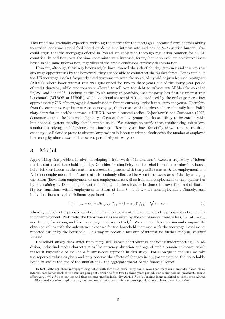
The empirical transition probabilities are obtained from empirical model as suggested by Mortensen andPissarides (1994) and developed recently by Shimer (2008). For the purpose of clarity, we only have twostates of the labour market status: employment and non-employment. Although flows into inactivity areconsiderable in Poland, cfr Figure (1), we assume that having a mortgage is a strong incentive to maintainactivity in the labour market. Therefore, we take the current aggregate inactivity rate as the maximumpossible and keep it constant throughout the simulation exercise3.

Figure 1: Source: Labour Force Surveys, 1995-2007

Consequently, implicitly any unemployment in our model is involuntary and any shock we model is aconsequence of changes in labour demand and not variability of household labour supply decisions. We de-cided to confine to employment and non-employment, because, from the perspective of households’ income,unemployment benefit and social assistance are comparable, while the key issue concerns the ability to earnincome sufficient to service mortgage payments.

In principle, flows between states should be described by two independent equations:

Et = (1− πN, t)Nt−1 + πE, tEt−1 − (1− πE, t)Et−1 (2)

Nt = πN, tNt−1 + (1− πE,t)Et−1 − (1− πN,t)Nt−1, (3)

which can subsequently be solved for πNtand πEt

. Consequently, using labour force survey data one canestablish these actual values for a chosen reference period.

Unfortunately, in practice there are two considerable difficulties with establishing relevant empiricalvalues for these parameters. First of all, there exists a large discontinuity problem when one uses actualPolish labour force data (large variability of estimators due to three significant changes in labour forcesurvey methodology). Therefore, actual data for period 1998-2001 (recent deterioration in labour marketoutlooks) have been smoothed. Secondly, creditor households differ noticeably from general population.Namely, they are more frequently employed and experience lower risk of being unemployed or inactive, cfrFigure (??). Imposing the values characteristic for the whole population would impose the risk of excessive

3Currently households budgets survey data are only available for 2007, so we consider 2007q4 inactivity rate to persist.

4

job loss hazard in the simulation. However, it would be difficult to justify any arbitrary adjustments inthese transition rates.

To overcome this former difficulty we have chosen the following empirical strategy. Firstly, we haveseparated the labour market status (and earnings) for each of the household members separately acrossthe households. This allows as to treat household members as individual labour market participants andcompute household revenues as a sum of individual earnings. The procedure for the separation is describedin the coming subsection.

The second step was to use propensity score matching technique to obtain relevant labour markettrajectories from the labour force survey. Namely, we used demographic, educational and geographicalcharacteristics to match members of creditor households obtained through household budgets survey withindividuals from labour force survey. For each of the points in time over the analysed period we haveobtained comparable unemployment, inactivity and employment rates, which provided reliable benchmarkfor simulations. This procedure is described in the following subsection.

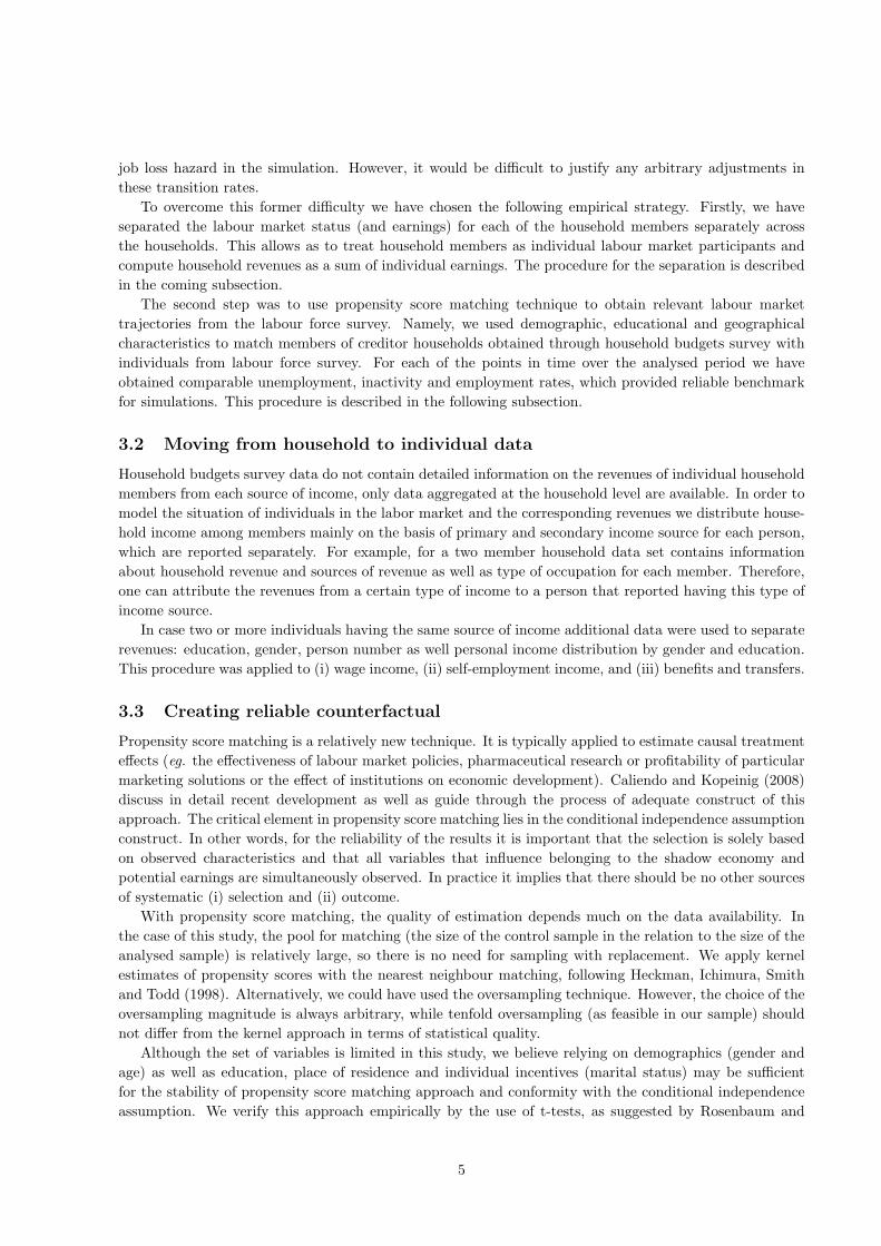
3.2 Moving from household to individual data

Household budgets survey data do not contain detailed information on the revenues of individual householdmembers from each source of income, only data aggregated at the household level are available. In order tomodel the situation of individuals in the labor market and the corresponding revenues we distribute house-hold income among members mainly on the basis of primary and secondary income source for each person,which are reported separately. For example, for a two member household data set contains informationabout household revenue and sources of revenue as well as type of occupation for each member. Therefore,one can attribute the revenues from a certain type of income to a person that reported having this type ofincome source.

In case two or more individuals having the same source of income additional data were used to separaterevenues: education, gender, person number as well personal income distribution by gender and education.This procedure was applied to (i) wage income, (ii) self-employment income, and (iii) benefits and transfers.

3.3 Creating reliable counterfactual

Propensity score matching is a relatively new technique. It is typically applied to estimate causal treatmenteffects (eg. the effectiveness of labour market policies, pharmaceutical research or profitability of particularmarketing solutions or the effect of institutions on economic development). Caliendo and Kopeinig (2008)discuss in detail recent development as well as guide through the process of adequate construct of thisapproach. The critical element in propensity score matching lies in the conditional independence assumptionconstruct. In other words, for the reliability of the results it is important that the selection is solely basedon observed characteristics and that all variables that influence belonging to the shadow economy andpotential earnings are simultaneously observed. In practice it implies that there should be no other sourcesof systematic (i) selection and (ii) outcome.

With propensity score matching, the quality of estimation depends much on the data availability. Inthe case of this study, the pool for matching (the size of the control sample in the relation to the size of theanalysed sample) is relatively large, so there is no need for sampling with replacement. We apply kernelestimates of propensity scores with the nearest neighbour matching, following Heckman, Ichimura, Smithand Todd (1998). Alternatively, we could have used the oversampling technique. However, the choice of theoversampling magnitude is always arbitrary, while tenfold oversampling (as feasible in our sample) shouldnot differ from the kernel approach in terms of statistical quality.

Although the set of variables is limited in this study, we believe relying on demographics (gender andage) as well as education, place of residence and individual incentives (marital status) may be sufficientfor the stability of propensity score matching approach and conformity with the conditional independenceassumption. We verify this approach empirically by the use of t-tests, as suggested by Rosenbaum and

5

Rubin (1983).In particular, we have performed two matching procedures. In the first version for each continuous

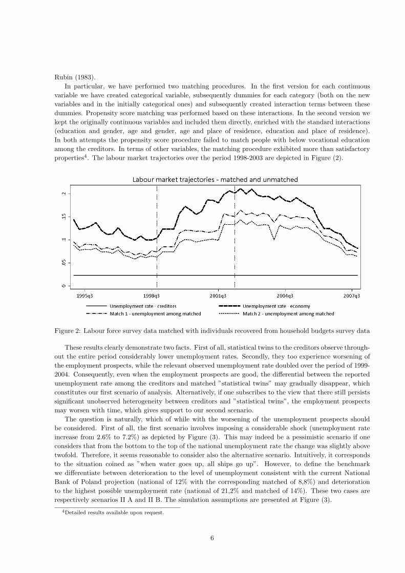
variable we have created categorical variable, subsequently dummies for each category (both on the newvariables and in the initially categorical ones) and subsequently created interaction terms between thesedummies. Propensity score matching was performed based on these interactions. In the second version wekept the originally continuous variables and included them directly, enriched with the standard interactions(education and gender, age and gender, age and place of residence, education and place of residence).In both attempts the propensity score procedure failed to match people with below vocational educationamong the creditors. In terms of other variables, the matching procedure exhibited more than satisfactoryproperties4. The labour market trajectories over the period 1998-2003 are depicted in Figure (2).

Figure 2: Labour force survey data matched with individuals recovered from household budgets survey data

These results clearly demonstrate two facts. First of all, statistical twins to the creditors observe through-out the entire period considerably lower unemployment rates. Secondly, they too experience worsening ofthe employment prospects, while the relevant observed unemployment rate doubled over the period of 1999-2004. Consequently, even when the employment prospects are good, the differential between the reportedunemployment rate among the creditors and matched ”statistical twins” may gradually disappear, whichconstitutes our first scenario of analysis. Alternatively, if one subscribes to the view that there still persistssignificant unobserved heterogeneity between creditors and ”statistical twins”, the employment prospectsmay worsen with time, which gives support to our second scenario.

The question is naturally, which of while with the worsening of the unemployment prospects shouldbe considered. First of all, the first scenario involves imposing a considerable shock (unemployment rateincrease from 2.6% to 7.2%) as depicted by Figure (3). This may indeed be a pessimistic scenario if oneconsiders that from the bottom to the top of the national unemployment rate the change was slightly abovetwofold. Therefore, it seems reasonable to consider also the alternative scenario. Intuitively, it correspondsto the situation coined as ”when water goes up, all ships go up”. However, to define the benchmarkwe differentiate between deterioration to the level of unemployment consistent with the current NationalBank of Poland projection (national of 12% with the corresponding matched of 8,8%) and deteriorationto the highest possible unemployment rate (national of 21,2% and matched of 14%). These two cases arerespectively scenarios II A and II B. The simulation assumptions are presented at Figure (3).

4Detailed results available upon request.

6

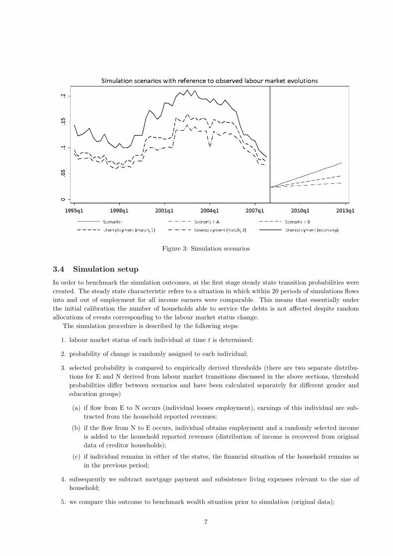
Figure 3: Simulation scenarios

3.4 Simulation setup

In order to benchmark the simulation outcomes, at the first stage steady state transition probabilities werecreated. The steady state characteristic refers to a situation in which within 20 periods of simulations flowsinto and out of employment for all income earners were comparable. This means that essentially underthe initial calibration the number of households able to service the debts is not affected despite randomallocations of events corresponding to the labour market status change.

The simulation procedure is described by the following steps:

1. labour market status of each individual at time t is determined;

2. probability of change is randomly assigned to each individual;

3. selected probability is compared to empirically derived thresholds (there are two separate distribu-tions for E and N derived from labour market transitions discussed in the above sections, thresholdprobabilities differ between scenarios and have been calculated separately for different gender andeducation groups)

(a) if flow from E to N occurs (individual looses employment), earnings of this individual are sub-tracted from the household reported revenues;

(b) if the flow from N to E occurs, individual obtains employment and a randomly selected incomeis added to the household reported revenues (distribution of income is recovered from originaldata of creditor households);

(c) if individual remains in either of the states, the financial situation of the household remains asin the previous period;

4. subsequently we subtract mortgage payment and subsistence living expenses relevant to the size ofhousehold;

5. we compare this outcome to benchmark wealth situation prior to simulation (original data);

7

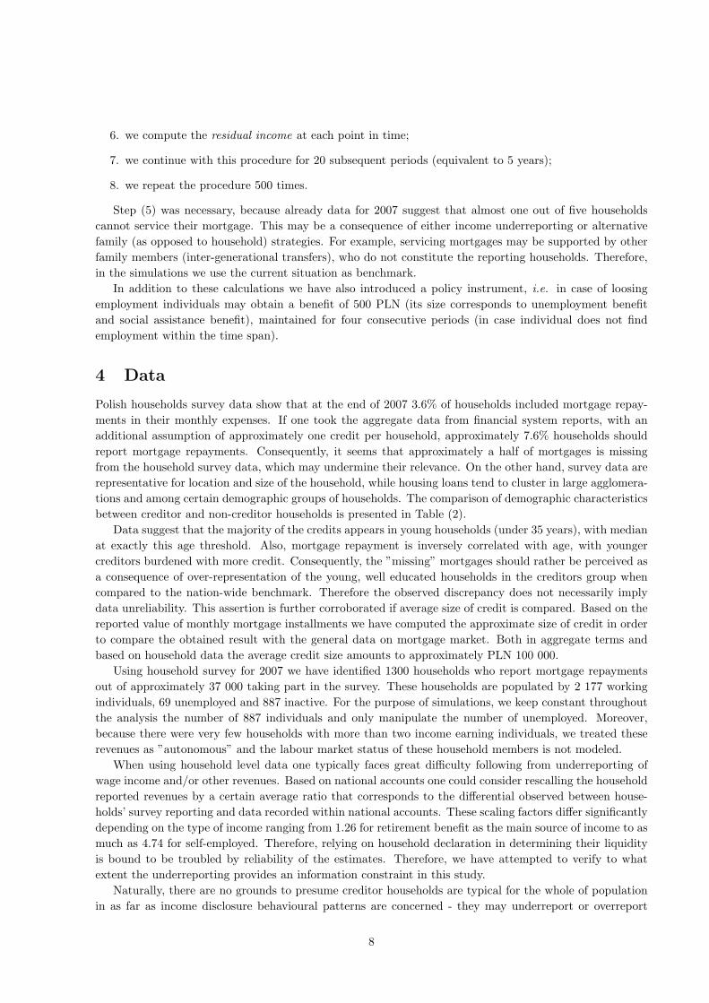
6. we compute the residual income at each point in time;

7. we continue with this procedure for 20 subsequent periods (equivalent to 5 years);

8. we repeat the procedure 500 times.

Step (5) was necessary, because already data for 2007 suggest that almost one out of five householdscannot service their mortgage. This may be a consequence of either income underreporting or alternativefamily (as opposed to household) strategies. For example, servicing mortgages may be supported by otherfamily members (inter-generational transfers), who do not constitute the reporting households. Therefore,in the simulations we use the current situation as benchmark.

In addition to these calculations we have also introduced a policy instrument, i.e. in case of loosingemployment individuals may obtain a benefit of 500 PLN (its size corresponds to unemployment benefitand social assistance benefit), maintained for four consecutive periods (in case individual does not findemployment within the time span).

4 Data

Polish households survey data show that at the end of 2007 3.6% of households included mortgage repay-ments in their monthly expenses. If one took the aggregate data from financial system reports, with anadditional assumption of approximately one credit per household, approximately 7.6% households shouldreport mortgage repayments. Consequently, it seems that approximately a half of mortgages is missingfrom the household survey data, which may undermine their relevance. On the other hand, survey data arerepresentative for location and size of the household, while housing loans tend to cluster in large agglomera-tions and among certain demographic groups of households. The comparison of demographic characteristicsbetween creditor and non-creditor households is presented in Table (2).

Data suggest that the majority of the credits appears in young households (under 35 years), with medianat exactly this age threshold. Also, mortgage repayment is inversely correlated with age, with youngercreditors burdened with more credit. Consequently, the ”missing” mortgages should rather be perceived asa consequence of over-representation of the young, well educated households in the creditors group whencompared to the nation-wide benchmark. Therefore the observed discrepancy does not necessarily implydata unreliability. This assertion is further corroborated if average size of credit is compared. Based on thereported value of monthly mortgage installments we have computed the approximate size of credit in orderto compare the obtained result with the general data on mortgage market. Both in aggregate terms andbased on household data the average credit size amounts to approximately PLN 100 000.

Using household survey for 2007 we have identified 1300 households who report mortgage repaymentsout of approximately 37 000 taking part in the survey. These households are populated by 2 177 workingindividuals, 69 unemployed and 887 inactive. For the purpose of simulations, we keep constant throughoutthe analysis the number of 887 individuals and only manipulate the number of unemployed. Moreover,because there were very few households with more than two income earning individuals, we treated theserevenues as ”autonomous” and the labour market status of these household members is not modeled.

When using household level data one typically faces great difficulty following from underreporting ofwage income and/or other revenues. Based on national accounts one could consider rescalling the householdreported revenues by a certain average ratio that corresponds to the differential observed between house-holds’ survey reporting and data recorded within national accounts. These scaling factors differ significantlydepending on the type of income ranging from 1.26 for retirement benefit as the main source of income to asmuch as 4.74 for self-employed. Therefore, relying on household declaration in determining their liquidityis bound to be troubled by reliability of the estimates. Therefore, we have attempted to verify to whatextent the underreporting provides an information constraint in this study.

Naturally, there are no grounds to presume creditor households are typical for the whole of populationin as far as income disclosure behavioural patterns are concerned - they may underreport or overreport

8

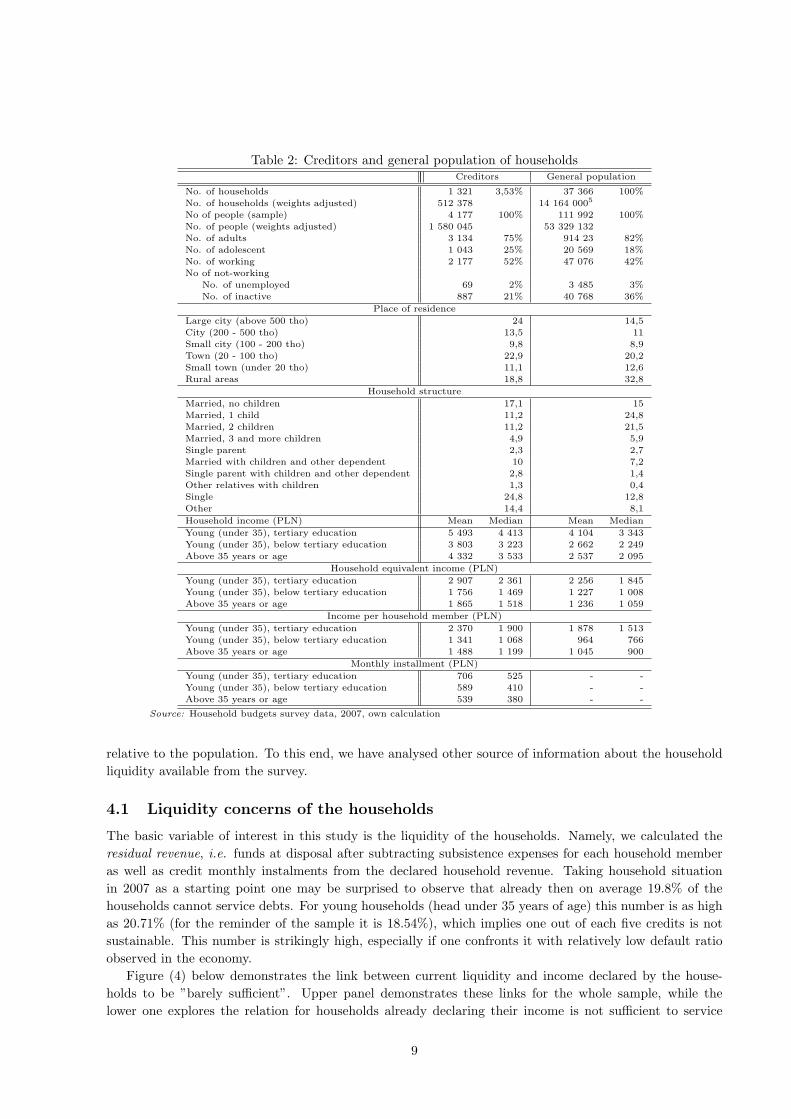
Table 2: Creditors and general population of householdsCreditors General population

No. of households 1 321 3,53% 37 366 100%

No. of households (weights adjusted) 512 378 14 164 0005

No of people (sample) 4 177 100% 111 992 100%

No. of people (weights adjusted) 1 580 045 53 329 132

No. of adults 3 134 75% 914 23 82%

No. of adolescent 1 043 25% 20 569 18%

No. of working 2 177 52% 47 076 42%

No of not-working

No. of unemployed 69 2% 3 485 3%

No. of inactive 887 21% 40 768 36%

Place of residence

Large city (above 500 tho) 24 14,5

City (200 - 500 tho) 13,5 11

Small city (100 - 200 tho) 9,8 8,9

Town (20 - 100 tho) 22,9 20,2

Small town (under 20 tho) 11,1 12,6

Rural areas 18,8 32,8

Household structure

Married, no children 17,1 15

Married, 1 child 11,2 24,8

Married, 2 children 11,2 21,5

Married, 3 and more children 4,9 5,9

Single parent 2,3 2,7

Married with children and other dependent 10 7,2

Single parent with children and other dependent 2,8 1,4

Other relatives with children 1,3 0,4

Single 24,8 12,8

Other 14,4 8,1

Household income (PLN) Mean Median Mean Median

Young (under 35), tertiary education 5 493 4 413 4 104 3 343

Young (under 35), below tertiary education 3 803 3 223 2 662 2 249

Above 35 years or age 4 332 3 533 2 537 2 095

Household equivalent income (PLN)


Young (under 35), below tertiary education 1 756 1 469 1 227 1 008

Above 35 years or age 1 865 1 518 1 236 1 059

Income per household member (PLN)


Young (under 35), below tertiary education 1 341 1 068 964 766

Above 35 years or age 1 488 1 199 1 045 900

Monthly installment (PLN)

Young (under 35), tertiary education 706 525 - -

Young (under 35), below tertiary education 589 410 - -

Above 35 years or age 539 380 - -

Source: Household budgets survey data, 2007, own calculation

relative to the population. To this end, we have analysed other source of information about the householdliquidity available from the survey.

4.1 Liquidity concerns of the households

The basic variable of interest in this study is the liquidity of the households. Namely, we calculated theresidual revenue, i.e. funds at disposal after subtracting subsistence expenses for each household memberas well as credit monthly instalments from the declared household revenue. Taking household situationin 2007 as a starting point one may be surprised to observe that already then on average 19.8% of thehouseholds cannot service debts. For young households (head under 35 years of age) this number is as highas 20.71% (for the reminder of the sample it is 18.54%), which implies one out of each five credits is notsustainable. This number is strikingly high, especially if one confronts it with relatively low default ratioobserved in the economy.

Figure (4) below demonstrates the link between current liquidity and income declared by the house-holds to be ”barely sufficient”. Upper panel demonstrates these links for the whole sample, while thelower one explores the relation for households already declaring their income is not sufficient to service

9

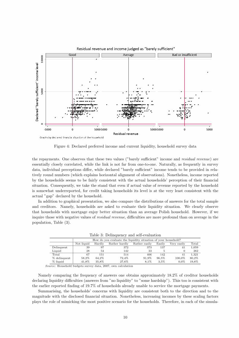
Figure 4: Declared preferred income and current liquidity, household survey data

the repayments. One observes that these two values (”barely sufficient” income and residual revenue) areessentially closely correlated, while the link is not far from one-to-one. Naturally, as frequently in surveydata, individual perceptions differ, while declared ”barely sufficient” income tends to be provided in rela-tively round numbers (which explains horizontal alignment of observations). Nonetheless, income reportedby the households seems to be fairly consistent with the actual households’ perception of their financialsituation. Consequently, we take the stand that even if actual value of revenue reported by the householdis somewhat underreported, for credit taking households its level is at the very least consistent with theactual ”gap” declared by the household.

In addition to graphical presentation, we also compare the distributions of answers for the total sampleand creditors. Namely, households are asked to evaluate their liquidity situation. We clearly observethat households with mortgage enjoy better situation than an average Polish household. However, if weinquire those with negative values of residual revenue, difficulties are more profound than on average in thepopulation, Table (3).

Table 3: Delinquency and self-evaluationHow do you evaluate the liquidity situation of your household?

Not liquid Hardly Rather hardly Rather easily Easily Very easily Total

Delinquent 39 97 372 373 137 41 1,059

Liquid 28 54 142 33 5 0 262

Total 67 151 514 406 142 41 1,321

% delinquent 58,2% 64,2% 72,4% 91,9% 96,5% 100,0% 80,2%

% liquid 41,8% 35,8% 27,6% 8,1% 3,5% 0,0% 19,8%

Source: Household budgets survey data, 2007, own calculation

Namely comparing the frequency of answers one obtains approximately 18.2% of creditor householdsdeclaring liquidity difficulties (answers from ”no liquidity” to ”some hardship”). This too is consistent withthe earlier reported finding of 19.7% of households already unable to service the mortgage payments.

Summarising, the households’ concerns with liquidity are consistent both to the direction and to themagnitude with the disclosed financial situation. Nonetheless, increasing incomes by these scaling factorsplays the role of mimicking the most positive scenario for the households. Therefore, in each of the simula-

10

tions both cases (corrected and raw income) are used. In our sample, a large share of households membersreport earnings from self-employment which leads to the difference in average scaling factor: it is 1.92 forthe creditors whereas in population it amounts to 1.71.

5 Results

This section reports the results of the simulations performed 500 times over 20 periods. We have takentwo perspectives to provide informative outcomes. First, we have observed the distributions of the residualrevenue, observing the percentile of the distribution for which households become delinquent under diversescenarios. Second, we used these results to provide estimates of the threat to the stability of the financialsystem depending on a scenario.

All results are reported in two variants. Namely, in the simulations all individuals moving from employ-ment to non-employment may obtain a benefit of 500 PLN (which is barely equivalent to the unemploymentbenefit in Poland). However, calculating the residual revenue we implicitly assume that household onlyallocates to consumption the so-called subsistence minimum6. In the real world, however, it is likely thatthe households experiencing the worsening of the financial situation will not be able to constrain previouslyhigher consumption to this very low level. Therefore, one should consider the ”no instrument” scenario torefer to a case where the households allocate unemployment benefit entirely to consumption not facilitatingmortgage servicing. Alternatively, ”instrument” scenario refers to a situation where the mortgage servicinghas strict priority over consumption and delinquency is the actual household’s condition7.

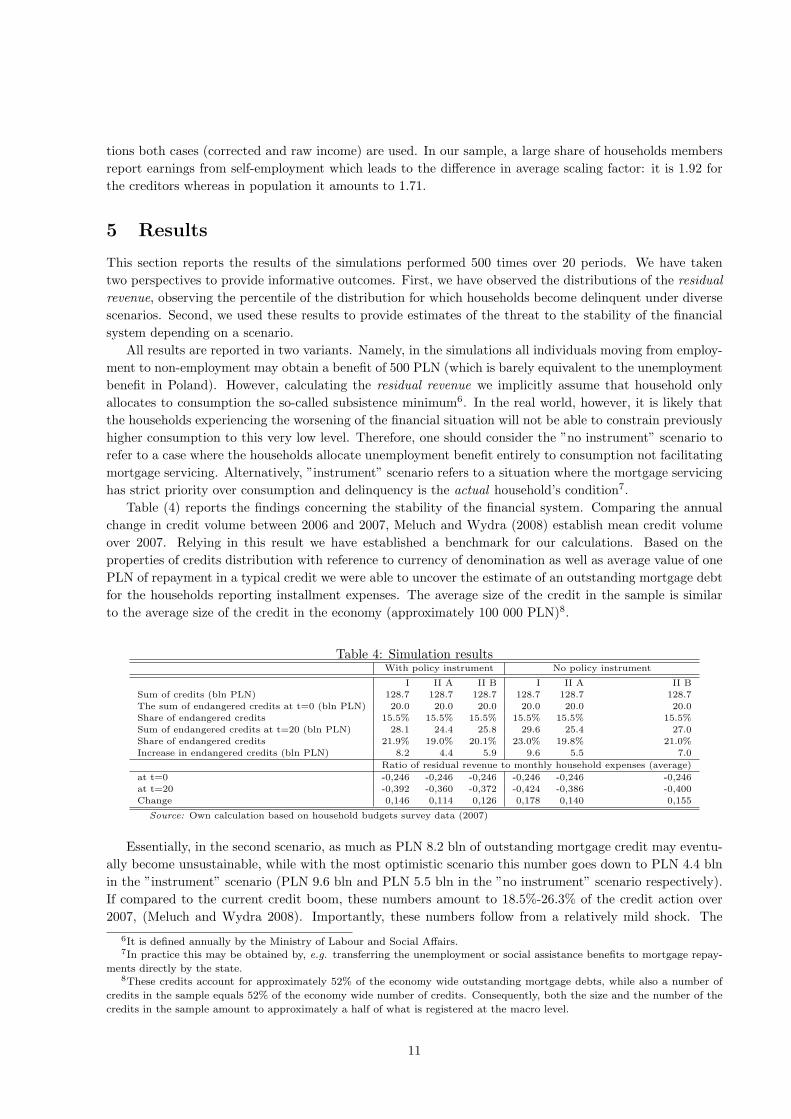
Table (4) reports the findings concerning the stability of the financial system. Comparing the annualchange in credit volume between 2006 and 2007, Meluch and Wydra (2008) establish mean credit volumeover 2007. Relying in this result we have established a benchmark for our calculations. Based on theproperties of credits distribution with reference to currency of denomination as well as average value of onePLN of repayment in a typical credit we were able to uncover the estimate of an outstanding mortgage debtfor the households reporting installment expenses. The average size of the credit in the sample is similarto the average size of the credit in the economy (approximately 100 000 PLN)8.

Table 4: Simulation resultsWith policy instrument No policy instrument

I II A II B I II A II B

Sum of credits (bln PLN) 128.7 128.7 128.7 128.7 128.7 128.7

The sum of endangered credits at t=0 (bln PLN) 20.0 20.0 20.0 20.0 20.0 20.0

Share of endangered credits 15.5% 15.5% 15.5% 15.5% 15.5% 15.5%

Sum of endangered credits at t=20 (bln PLN) 28.1 24.4 25.8 29.6 25.4 27.0

Share of endangered credits 21.9% 19.0% 20.1% 23.0% 19.8% 21.0%

Increase in endangered credits (bln PLN) 8.2 4.4 5.9 9.6 5.5 7.0

Ratio of residual revenue to monthly household expenses (average)

at t=0 -0,246 -0,246 -0,246 -0,246 -0,246 -0,246

at t=20 -0,392 -0,360 -0,372 -0,424 -0,386 -0,400

Change 0,146 0,114 0,126 0,178 0,140 0,155

Source: Own calculation based on household budgets survey data (2007)

Essentially, in the second scenario, as much as PLN 8.2 bln of outstanding mortgage credit may eventu-ally become unsustainable, while with the most optimistic scenario this number goes down to PLN 4.4 blnin the ”instrument” scenario (PLN 9.6 bln and PLN 5.5 bln in the ”no instrument” scenario respectively).If compared to the current credit boom, these numbers amount to 18.5%-26.3% of the credit action over2007, (Meluch and Wydra 2008). Importantly, these numbers follow from a relatively mild shock. The

6It is defined annually by the Ministry of Labour and Social Affairs.7In practice this may be obtained by, e.g. transferring the unemployment or social assistance benefits to mortgage repay-

ments directly by the state.8These credits account for approximately 52% of the economy wide outstanding mortgage debts, while also a number of

credits in the sample equals 52% of the economy wide number of credits. Consequently, both the size and the number of the

credits in the sample amount to approximately a half of what is registered at the macro level.

11

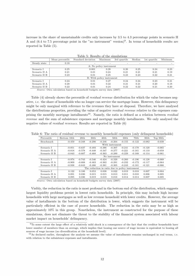
increase in the share of unsustainable credits only increases by 3.5 to 4.3 percentage points in scenario IIA and (6.4 to 7.5 percentage point in the ”no instrument” version)9. In terms of households results arereported in Table (5).

Table 5: Results of the simulationsMean percentile Standard deviation Maximum 3rd quartile Median 1st quartile Minimum

Steady state 0.18 - - - - - -

A: No policy instrument

Scenario I 0.25 0.001 0.28 0.26 0.25 0.24 0.23

Scenario II A 0.21 0.01 0.24 0.21 0.21 0.21 0.19

Scenario II B 0.23 0.01 0.25 0.23 0.23 0.22 0.21

B: With policy instrument

Scenario I 0.24 0.01 0.27 0.24 0.24 0.23 0.21

Scenario II A 0.20 0.01 0.22 0.21 0.21 0.20 0.18

Scenario II B 0.22 0.01 0.24 0.22 0.22 0.21 0.20


Table (4) already shows the percentile of residual revenue distribution for which the value becomes neg-ative, i.e. the share of households who no longer can service the mortgage loans. However, this delinquencymight be only marginal with reference to the revenues they have at disposal. Therefore, we have analysedthe distributions properties, providing the value of negative residual revenue relative to the expenses com-prising the monthly mortgage installments10. Namely, the ratio is defined as a relation between residualrevenue and the sum of subsistence expenses and mortgage monthly installments. We only analysed thenegative values of residual revenues. Results are reported in Table (6)

Table 6: The ratio of residual revenue to monthly household expenses (only delinquent households)Percentile Bottom 10th 20th 30th 40th 50th 60th 70th 80th Top 90th

Benchmark -0.459 -0.348 -0.290 -0.246 -0.204 -0.155 -0.122 -0.082 -0.039

With instrument

Scenario I -0.851 -0.637 -0.493 -0.386 -0.307 -0.241 -0.178 -0.120 -0.065

Scenario II A -0.818 -0.578 -0.448 -0.347 -0.277 -0.221 -0.161 -0.110 -0.059

Scenario II B -0.843 -0.607 -0.468 -0.363 -0.289 -0.229 -0.168 -0.114 -0.061

No instrument

Scenario I -0.974 -0.743 -0.546 -0.424 -0.329 -0.260 -0.196 -0.128 -0.068

Scenario II A -0.909 -0.608 -0.463 -0.362 -0.291 -0.232 -0.172 -0.117 -0.064

Scenario II B -0.938 -0.643 -0.486 -0.381 -0.305 -0.243 -0.181 -0.121 -0.066

The reduction in ratio due to policy instrument

Scenario I 0.122 0.106 0.053 0.038 0.022 0.019 0.018 0.007 0.004

Scenario II A 0.091 0.030 0.015 0.015 0.013 0.011 0.010 0.006 0.005

Scenario II B 0.095 0.036 0.019 0.018 0.016 0.014 0.014 0.007 0.005


Visibly, the reduction in the ratio is most profound in the bottom end of the distribution, which suggestslargest liquidity problems persist in lowest ratio households. In principle, this may include high incomehouseholds with large mortgages as well as low revenue household with lower credits. However, the averagevalue of installments in the bottom of the distribution is lower, which suggests the instrument will beparticularly efficient in the case of poorer households. The reduction in the ratio may be as high asapproximately 10% in this group. Nonetheless, the instrument as constructed for the purpose of thesesimulations, does not eliminate the threat to the stability of the financial system associated with labourmarket impact on households’ delinquency.

9To some extent the large effect of a relatively mild shock is a consequence of the fact that the creditor households have

lower number of members than on average, which implies that loosing one source of wage income is equivalent to loosing all

sources of wage income (no diversification at the household level).10As declared earlier, throughout the analysis we assume the value of installments remains unchanged in real terms, i.e.

with relation to the subsistence expenses and installments.

12

6 Concluding remarks

Subprime crisis which originated in the US spread to many countries via the financial integration links.Monetary and fiscal authorities in many countries ponder about the ways of immuning the economy tothe spreading of the crisis. In this paper we attempted to test if using the household survey data -typically available in all the developed economies - one can actually evaluate a risk of breeding one’s ownsubprime crisis instead. We find that even with relatively small number of creditors (in the Polish economyonly approximately 7.6% of households have a mortgage) the actually effects of deteriorating the financialsituation among the debtors can be indeed sizeable.

We use simulations in order to observe the impact on household liquidity derived from two alternativescenarios. In the first, we explicitly model the deterioration of labour market status due to, for example,economic slowdown. In the latter, we observe the consequences of creditors gradually resembling theircounterparts within respective subgroups of the population in terms of labour market performance. Inboth cases we find that even small changes in the employment persistence or unemployment risk canlead to considerable deterioration of households’ liquidity and therefore the financial stability of the wholemortgage market. Please note, that in simulation we do not allow for the bank intervention (e.g. sellingof the property, relieving the monthly installments, etc.). Naturally, observing lowering ability to repaythe debts bank may engage into cooperating with the clients on designing tailored solutions. On the otherhand, having the large number of agents in the simulation, this model outcomes hold by the token ofstatistics. Finding future creditors with better labour market outlooks will not be statistically feasible ifthe assumptions of our model hold and the simulation scenarios are relevant.

There are few issues we did not cover in the model. Firstly, already in 2007 a large share of householdswould not be able to service mortgage payments - 20% for raw income data and 9% if income reported bythe households was corrected using benchmark values obtained from the national accounts. This is at oddswith endangered credit volumes reported by the banks - at the end of 2007 approximately 1% of credits,(Meluch and Wydra 2008). We seek the roots of this situation in the fact that many young creditorsmay actually benefit from the support of their families. Alternatively, some underreported employment(gray economy) may matter for the liquidity of the households. None of these issues may be tackled usinghousehold survey data, however.

References

Barwell, R., Orla, M. and Pezzini, S.: 2006, The Distribution of Assets, Income and Liabilities Across UKHouseholds: Results From the 2005 NMG Research Survey, Technical report, Bank of England.

Caliendo, M. and Kopeinig, S.: 2008, Some Practical Guidance For The Implementation Of PropensityScore Matching, Journal of Economic Surveys 22(1), 31–72.

Faraqui, U.: 2006, Are There Significant Disparities in Debt Burden Across Canadian Households? AnExamination of the Distribution of the Debt Service Ratio Using Micro Data, Measuring the FinancialPosition of the Household Sector, Vol. 2, IFC Bulletin .

Gorton, G. B.: 2008, The Subprime Panic, NBER Working Papper 14398, National Bureau of EconomicResearch.

Heckman, J., Ichimura, H., Smith, J. and Todd, P.: 1998, Characterizing Selection Bias Using ExperimentalData, Econometrica 66(5), 1017–1098.

Johansson, M. W. and Persson, M.: 2006, Swedish Households’ Indebtedness and Ability To Pay – aHousehold Level Study, Measuring the Financial Position of Household Sector, Vol. 2, IFC Bulletin.

Meluch, B. and Wydra, M.: 2008, Rynek finansowania nieruchomosci mieszkaniowych w Polsce - stan na30 czerwca 2008r (Financing of Real Estate in Poland, June 2008 ), Finansowanie nieruchomosci .

13

Mortensen, D. T. and Pissarides, C. A.: 1994, Job Creation and Job Destruction in the Theory of Unem-ployment, Review of Economic Studies 61(3), 397–415.

Osinski, J., Szpunar, P. and Tymoczko (eds.), D.: 2008, Raport o stabilnosci systemu finansowego (reporton the financial system stability), National Bank of Poland, semi-annual report. Frame 2, p. 43.

Rosenbaum, P. and Rubin, D.: 1983, The Central Role of the Propensity Score in Observational Studiesfor Causal Effects, Biometrika 70(1), 41–55.

Shimer, R.: 2008, The Probability of Finding a Job, American Economic Review 98(2), 268–73.

Simigiannis, G. T. and Tzamourani, P.: 2006, Greek Household Indebtedness and Financial Stress Resultsfrom Household Survey Data, Measuring the Financial Position of the Household Sector, Vol. 2, IFCBulletin .

Wagner, H.: 2004, The Use Of Credit Scoring In The Mortgage Industry , Journal of Financial ServicesMarketing 9(2), 179–183.

Zajaczkowski, S. and Zochowski, D.: 2007, Obciazenie gospodarstw domowych splatami dlugow: rozkladyi stress testy na podstawie badan budzetow gospodarstw domowych gus (household indebtedness:Distributions and stress tests based on household budgets survey data), Materialy i Studia (Analysesand Studies) 212, National Bank of Poland.

14

Documents

Breeding Ones’ Own Subprime Crisis