BREEDING ECOLOGY, SURVIVAL RATES, AND CAUSES OF MORTALITY

OF HUNTED AND NONHUNTED GREATER SAGE-GROUSE

IN CENTRAL MONTANA

by

Jenny Lyn Sika

A thesis submitted in partial fulfillment of the requirements for the degree

of

Master of Science

in

Fish and Wildlife Management

MONTANA STATE UNIVERSITY Bozeman, Montana

November 2006

© COPYRIGHT

by

Jenny Lyn Sika

2006

All Rights Reserved

ii

APPROVAL

of a thesis submitted by

Jenny Lyn Sika

This thesis has been read by each member of the thesis committee and has been found to

be satisfactory regarding content, English usage, format, citations, bibliographic style,

and consistency, and is ready for submission to the Division of Graduate Education.

Dr. Jay J. Rotella, Committee Chair

Approved for the Department of Ecology

Dr. David Roberts, Department Chair

Approved for the Division of Graduate Education

Dr. Carl A. Fox, Vice Provost

iii

STATEMENT OF PERMISSION TO USE

In presenting this thesis in partial fulfillment of the requirements for a master’s

degree at Montana State University, I agree that the Library shall make it available to

borrowers under rules of the Library. I further agree that copying of this thesis is

allowable only for scholarly purposes, consistent with “fair use” as prescribed in the U.S.

Copyright Law. Requests for extensive copying or reproduction of this thesis may be

granted by the copyright holder.

Jenny Lyn Sika November 2006

iv

ACKNOWLEDGEMENTS

I extend sincere thanks to the many biologists (FWP, BLM, MSU, & UM) that

contributed in innumerable ways to this project. Jay Newell mentored and teased me and was

a positive force throughout. Jay Watson provided much technical ingenuity and was a

nightlighting machine. Allison Puchniak-Begley trapped birds and befriended me at the

beginning. At all hours of the night, Sean Stewart, Clair Simmons, Ray Mule’, Gary Dusek,

Dave Pac, and Tom Lehmke all trapped birds and provided comic relief. Charlie Eustace

radio-tracked birds overwinter. Neil Anderson, Mark Atkinson, Jeff Herbert, Keith Aune,

Kurt Alt, Rick Northrup, and Lydia Bailey provided logistical support, equipment, and

expertise. Lee Burroughs and Dale Nixdorf assisted with trapping and/or tracking and

provided landowner information and hunter data. Jay Parks made the habitat work possible.

I extend thanks and appreciation to my committee. Jay Rotella, my advisor, encouraged

me to always be critical in my scientific thinking and doing, and his approach to mentoring

was outstanding. Bob Garrott provided critical feedback and helped me improve my writing.

Carl Wambolt was instrumental in getting the sagebrush-habitat work off the ground.

B. Sowell collaborated with the habitat work. V. Lane and J. Woodward conducted

graduate research of sagebrush habitats. J. Woodward also monitored birds overwinter. B.

Moynahan got me started with protocols and datasheets. H. Harrison made us movie stars.

M. Richman, A. Anderson, S. Conner, D. Auerbach, D. Keto, M. Peters, M. Watrobka, K.

Drake, and A. Torrick were the muscles of this project. S. Conner and D. Keto also

conducted undergraduate research of artificial nests and sage-grouse males, respectively.

Finally, I extend a tremendous thanks to Brett Walker, who shared his enthusiasm for

biology and hours and hours of sage-grouse shop talk, reviewed several versions of my

thesis, cooked many meals, gave me hugs and encouragement, and walked with me.

v

TABLE OF CONTENTS LIST OF TABLES...................................................................................................... vii LIST OF FIGURES ...................................................................................................... x ABSTRACT................................................................................................................. xi 1. INTRODUCTION ........................................................................................................ 1 Introduction to Thesis ....................................................................................................1 Literature Cited ............................................................................................................. 4 2. BREEDING ECOLOGY OF GREATER SAGE-GROUSE IN CENTRAL

MONTANA .................................................................................................................. 6 Introduction....................................................................................................................6 Study Area .....................................................................................................................9 Methods........................................................................................................................11 Nesting .................................................................................................................. 14 Brood-Rearing....................................................................................................... 15 Data Analysis ........................................................................................................ 15 Nesting Probability, Renesting Probability, and Reproductive Success......... 17 Nest Survival................................................................................................... 18 Brood Survival ................................................................................................ 19 Female Survival .............................................................................................. 19 Results..........................................................................................................................22 Nest Survival......................................................................................................... 24 Brood Survival ...................................................................................................... 27 Female Survival and Causes of Mortality............................................................. 29 Nesting-Season Survival................................................................................. 29 Late-Summer Survival .................................................................................... 33 Discussion....................................................................................................................37 Reproductive Effort .............................................................................................. 37 Nest Survival......................................................................................................... 38 Brood Survival ...................................................................................................... 41 Female Survival .................................................................................................... 43 Nesting-Season Survival................................................................................. 43 Late-Summer Survival .................................................................................... 46 Future Research .......................................................................................................... 47 Literature Cited ........................................................................................................... 49

vi

TABLE OF CONTENTS CONTINUED

3. FALL AND WINTER SURVIVAL RATES AND CAUSES OF MORTALITY

AMONG HUNTED AND NONHUNTED GREATER SAGE-GROUSE IN CENTRAL MONTANA............................................................................................. 55

Introduction..................................................................................................................55 Study Area ...................................................................................................................59 Methods........................................................................................................................62 Nesting and Brood-Rearing .................................................................................. 65 Hunting Season ..................................................................................................... 65 Overwinter ............................................................................................................ 66 Data Analysis ........................................................................................................ 66 Hunting-Season Survival ................................................................................ 68 Overwinter Survival........................................................................................ 69 Results..........................................................................................................................70 Hunting-Season Survival ...................................................................................... 70 Overwinter Survival.............................................................................................. 78 Discussion....................................................................................................................82 Hunting-Season Survival. ..................................................................................... 82 Overwinter Survival.............................................................................................. 88 Seasonal and Annual Survival Summary.............................................................. 89 Future Research .......................................................................................................... 91 Literature Cited ........................................................................................................... 94 4. CONCLUSION TO THESIS.................................................................................... 100 Extended Abstract......................................................................................................100 APPENDICES ................................................................................................................ 104 APPENDIX A: Map and Cover Types of Study Area in Central Montana..............105 APPENDIX B: Precipitation and Palmer Drought Severity Index for Central

Montana. ....................................................................................................................108 APPENDIX C: Unpublished Greater Sage-Grouse Lek Count Data in

Musselshell and Golden Valley Counties from Montana Fish, Wildlife and Parks, 1993-2005. ......................................................................................................112

APPENDIX D: Seasons for Survival Analyses in Central Montana during 2004-05. .....................................................................................................................115

APPENDIX E: 2003 Field Season............................................................................117

vii

LIST OF TABLES

Table Page

2.1. Observed nesting probabilities and renesting probabilities for yearling and adult sage grouse females and reproductive success in Musselshell and Golden Valley counties, Montana during 2004-05.................................................................................................25

2.2. Observed nesting probabilities and renesting probabilities for

yearling and adult sage grouse females excluding females that may have abandoned first nests due to investigator activity in Musselshell and Golden Valley counties, Montana during 2004-05.. ..........................................................................................................25

2.3. Number, fate, and apparent causes of failure of sage grouse nests

in Musselshell and Golden Valley counties, Montana during 2004-05. ...........................................................................................................25

2.4. Sample sizes included in survival analysis of sage grouse nests,

broods, and females during nesting and late-summer listed by year, site, total, and number of individual females in Musselshell and Golden Valley counties, Montana during 2004-05.. ..........................................................................................................26

2.5. A priori models of Daily Survival Rate (DSR) for sage-grouse

nests in Musselshell and Golden Valley counties, Montana during 2004-05.................................................................................................27

2.6. Maximum-likelihood (logit-link) estimates of beta parameters

from competing Daily Survival Rate (DSR) models for sage grouse nests in Musselshell and Golden Valley counties, Montana during 2004-05..................................................................................27

2.7. A priori models of Daily Survival Rate (DSR) for sage-grouse

broods in Musselshell and Golden Valley counties, Montana during 2004-05.................................................................................................28

2.8. Number of mortalities listed by year and site for each season and

suspected causes of mortality by season for sage grouse females in Musselshell and Golden Valley counties, Montana during 2004-05.................................................................................................31

viii

LIST OF TABLES CONTINUED

Table Page

2.9. A priori models of Daily Survival Rate (DSR) for sage grouse females during the nesting season in Musselshell and Golden Valley counties, Montana during 2004-05......................................................32

2.10. Maximum-likelihood (logit-link) estimates of beta parameters

from competing Daily Survival Rate (DSR) models for sage grouse females during the nesting season in Musselshell and Golden Valley counties, Montana during 2004-05.........................................33

2.11. A priori models of Daily Survival Rate (DSR) for sage grouse

females during late summer in Musselshell and Golden Valley counties, Montana during 2004-05. .................................................................35

2.12. Covariate coefficient estimates, standard errors, and 95%

confidence intervals for the best approximating model of late-summer survival of sage grouse in Musselshell and Golden Valley counties, Montana during 2004-05......................................................36

2.13. Monthly survival estimates during late summer from the best

approximating model for sage grouse females in Musselshell and Golden Valley counties, Montana during 2004-05. ..................................36

3.1. Sample sizes included in survival analysis of sage grouse females

for fall and winter by year, site, total, and individual females in Musselshell and Golden Valley counties, Montana during 2004-05 ............................................................................................................72

3.2. Number of mortalities listed by year and site for each season and

suspected causes of mortality by season in Musselshell and Golden Valley counties, Montana during 2004-05..........................................72

3.3. A priori models of Daily Survival Rate (DSR) ranked by

differences in AICc values for sage grouse females during the hunting season in Musselshell and Golden Valley counties, Montana during 2004-05..................................................................................75

ix

LIST OF TABLES CONTINUED

Table Page

3.4. Parameter estimates, standard errors, and 95% confidence intervals for the best approximating model, Nonhunted + Hunted * Trend3 + Days Rearing (single intercept model), of hunting-season survival of sage grouse in Musselshell and Golden Valley counties, Montana during 2004-05..........................................77

3.5. Parameter estimates, standard errors, and 95% confidence

intervals for the second best approximating model, Nonhunted + Hunted * Trend3 + Days Rearing (a model with two intercepts), of hunting season survival of sage grouse in Musselshell and Golden Valley counties, Montana during 2004-05 ............................................................................................................77

3.6. A priori models of Daily Survival Rate (DSR) for sage grouse

females overwinter in Musselshell and Golden Valley counties, Montana during 2004-05..................................................................................80

3.7. Summary of survival estimates from the best-supported models

for each season, annual survival estimates, and mean life span according to year, site, and number of days spent rearing a brood for sage grouse females in Musselshell and Golden Valley counties, Montana during 2004-05.......................................................82

x

LIST OF FIGURES

Figure Page 3.1. Hunting-season survival estimates (61 days) for sage grouse females

by number of days spent rearing a brood for a hunted and nonhunted population in Musselshell and Golden Valley counties, Montana during 2004-05. Estimates of hunting-season survival rate are based on estimates from the best model, and the averages and 95% CI values were obtained using parametric bootstrapping ......................78

xi

ABSTRACT

Declines in productivity have been implicated in population declines for greater sage-grouse (Centrocercus urophasianus) in several areas, but there is considerable variation in reproductive effort, reproductive success and female survival, both temporally and spatially, and more data are needed. Despite declining populations, sage grouse are still legally harvested in most of their current range, including Montana, and uncertainty about how harvest impacts sage grouse vital rates remains. The reproductive activity, survival rates, and causes of mortality of hunted and nonhunted sage grouse females were monitored year round using radio-telemetry in central Montana during 2004 and 2005. Data on nest survival and brood survival were also collected. Nest survival was greater for renests, 0.56, than for first nests, 0.32. Brood survival to 30 days post-hatch was estimated as 0.79. Reproductive effort and reproductive success were higher in 2005. Female survival during the nesting season was constant, 0.94 monthly. Female survival during July of both years was similar on both sites, 0.99 to nearly 1.00, but survival was lower during August and declined between 2004 and 2005 from 0.94 to 0.84 on the hunted site and declined from 0.98 to 0.94 on the nonhunted site. This decline in survival between years in August was likely due to West Nile virus, as it was first detected in sage grouse in this area in August 2005. Female survival during the hunting season was lower for females that spent more days brood-rearing than those that spent few or no days brood rearing, and females on the hunted site had lower survival than females on the nonhunted site. However, lower survival rates on the hunted site could not be attributed to hunter kill, because no radio-marked females were bagged or reported by hunters and no evidence of hunter kill was observed. During the hunting season, monthly survival estimates ranged from 0.87 for hunted-site females that invested heavily in brood rearing to 0.99 for nonhunted-site females that invested little or no time in brood rearing. Overwinter survival was different between years, and monthly survival during winter 2004-05 was estimated as 0.98 and as 0.97 during winter 2005-06.

1

CHAPTER ONE

INTRODUCTION

Introduction to Thesis

Greater sage-grouse (Centrocercus urophasianus), hereafter sage grouse,

populations have been declining throughout their historical range in western North

America since the early 1900s (Hornaday 1916), with current abundance estimated at 1-

31% of the numbers present prior to European settlement in the 1800s (United States Fish

and Wildlife Service 2004). In addition to a dramatic decline in abundance, sage grouse

distribution has contracted by as much as 44% (Schroeder et al. 2004).

Declines in productivity have been implicated in population declines in areas of

Colorado, Idaho, Montana, Oregon, Wyoming, and Alberta (e.g., Crawford and Lutz

1985, Connelly and Braun 1997, Connelly et al. 2004, Aldridge 2005), but there is

considerable variation in reproductive effort, reproductive success (productivity), and

female survival (see Schroeder 1997, Schroeder et al. 1999 and Connelly et al. 2000a,

2004 for review), both temporally and spatially. Reproductive effort and reproductive

success may be somewhat counterbalanced by opposite (or negatively covarying) levels

of female survival, and this counterbalance may stabilize population growth rates.

Therefore, it is important to study both reproduction and survival across years to obtain a

more accurate picture of how vital rates influence fluctuations in populations.

Despite declining populations, sage grouse are still legally harvested in most of

their current range, including Montana. Although there is currently a need to reduce

2

sources of mortality for sage grouse, harvest is also an incentive for conservation.

Licensing fees provide revenue for management of harvestable population sizes, and

hunting maintains public interest in game species. Uncertainty about how harvest

impacts sage grouse vital rates remains. Thus far, published research investigating the

effects of harvest on sage grouse vital rates has suggested that harvest mortality may not

be compensatory (Johnson and Braun 1999, Connelly et al. 2000b, Connelly et al. 2003)

or in contrast, has reported that hunting has little impact on populations (Wallestad 1975,

Crawford 1982, Braun and Beck 1985). Further, harvest may impact sage grouse

populations differently across their range, and thus, area-specific data on the impact of

harvest, and the magnitude of this impact relative to other potential sources of mortality,

are necessary for informed management.

Information from areas where sage grouse populations appear to be doing well

(i.e., where abundance is relatively high) may be valuable to understanding range-wide

declines and subsequently informing future research needs and management decisions.

This study was designed with the following objectives: 1) to estimate nesting and

renesting probabilities, nest survival, brood survival, and female survival for breeding

sage grouse with relatively healthy, robust populations on two sites in central Montana,

2) to simultaneously compare survival rates during the hunting season and overwinter

between adjacent hunted and nonhunted sites with similar landscape and population

characteristics, 3) to evaluate factors other hunting that influence survival during the

hunting season, 4) to assess the relative importance of different sources of mortality on

sage grouse during the hunting season and overwinter, and 5) to assess, to the extent

possible, the influence of harvest on the sage grouse populations studied and to make

3

recommendations for future investigations about the effects of harvest on sage grouse.

Breeding ecology is the subject of Chapter 2, and Chapter 3 discusses my research on

harvest and mortality causes.

4

Literature Cited

Aldridge, C. L. 2005. Identifying habitats for persistence of greater sage-grouse

(Centrocercus urophasianus) in Alberta, Canada. Dissertation, University of Alberta, Edmonton, Alberta, Canada.

Braun, C. E., and T. D. I. Beck. 1985. Effects of changes in hunting regulations on Sage Grouse harvest and populations. Pages 335-343 in S. L. Beasom and S. F. Roberson, editors. Game Harvest Management. Caesar Kleberg Wildlife Research Institute, Kingsville, Texas.

Connelly, J.W. and C.E. Braun. 1997. Long-term changes in Sage Grouse Centrocercus urophasianus populations in western North America. Wildlife Biology 3:229-234.

Connelly, J. W., M.A. Schroeder, A. R. Sands, and C. E. Braun. 2000a. Guidelines to manage sage grouse populations and their habitats. Wildlife Society Bulletin 28: 967-985.

Connelly, J. W., A. D. Apa, R. B. Smith, and K. P. Reese. 2000b. Effects of predation and hunting on adult sage grouse Centrocercus urophasianus in Idaho. Wildlife Biology 6: 227-232.

Connelly, J. W., K. P. Reese, E. O. Garton, and M. L. Commons-Kemner. 2003. Response of greater sage-grouse Centrocercus urophasianus populations to different levels of exploitation in Idaho, USA. Wildlife Biology 9:255-260.

Connelly, J. W., S. T. Knick, M. A. Schroeder, and S. J. Stiver. 2004. Conservation Assessment of Greater Sage-grouse and Sagebrush Habitats. Western Association of Fish and Wildlife Agencies. Unpublished Report. Cheyenne, Wyoming.

Crawford, J. A. 1982. Factors affecting sage grouse harvest in Oregon. Wildlife Society Bulletin 10:374-377.

Crawford, J. A., and R. S. Lutz.1985. Sage grouse population trends in Oregon, 1941–1983. The Murrelet 66:69-74.

Hornaday, W. T. 1916. Save the sage grouse from extinction, a demand from civilization to the western states. New York Zoological Park Bulletin 5:179-219.

Johnson, K. H. and C. E. Braun. 1999. Viability and conservation of an exploited sage grouse population. Conservation Biology 13:77-84.

U.S. Fish and Wildlife Service. 2004. 30-day finding for petitions to list the greater sage-grouse as threatened or endangered. Federal Registry 69(77):21484-21494.

5

Schroeder, M. A. 1997. Unusually high reproductive effort by sage grouse in a fragmented habitat in north-central Washington. The Condor 99:933-941.

Schroeder, M. A., J. R. Young, and C. E. Braun. 1999. Sage grouse (Centrocercus urophasianus). Pages 1-28 in A. Poole and F. Gill, editors. The Birds of North America, Number 425. The Birds of North America, Inc., Philadelphia, Pennsylvania, USA.

Schroeder, M. A., C. L. Aldridge, A. D. Apa, J. R. Bohne, C. E. Braun, S. D. Bunnell, J. W. Connelly, P. A. Deibert, S. C. Gardner, M. A. Hilliard, G. D. Kobriger, S. M. McAdam, C. W. McCarthy, J. J. McCarthy, D. L. Michell, E. V. Rickerson and S. J. Stiver. 2004. Distribution of sage-grouse in North America. The Condor 106:363-376.

Wallestad, R. 1975. Montana sage grouse. Montana Department of Fish and Game and United States Bureau of Land Management, Helena, Montana, USA.

6

CHAPTER TWO

BREEDING ECOLOGY OF GREATER SAGE-GROUSE IN CENTRAL MONTANA

Introduction

Greater sage-grouse (Centrocercus urophasianus; hereafter, sage grouse)

populations have been declining throughout their historical range in western North

America since the early 1900s (Hornaday 1916), with current abundance estimated at 1-

31% of the numbers present prior to European settlement in the 1800s (United States Fish

and Wildlife Service 2004). In addition to a dramatic decline in abundance, sage grouse

distribution has contracted by as much as 44% (Schroeder et al. 2004). As of 1997,

populations were considered secure in Idaho, Wyoming, Oregon, Nevada, and Montana

(Connelly and Braun 1997). Currently, populations in Colorado, Utah, California,

Washington, and Nevada are considered the most isolated (Connelly et al. 2004). Much

of central Montana is still in relatively contiguous sagebrush-steppe habitat, supports

relatively large numbers of sage grouse, and supports populations that appear to be

relatively stable at the present time (Connelly et al. 2004, Montana Sage Grouse Work

Group 2005). Declines in productivity have been implicated in population declines in

areas of Colorado, Idaho, Montana, Oregon, Wyoming, and Alberta (e.g., Crawford and

Lutz 1985, Connelly and Braun 1997, Connelly et al. 2004, Aldridge 2005), but there is

considerable variation in reproductive effort, reproductive success (productivity), and

female survival (see Schroeder 1997, Schroeder et al. 1999 and Connelly et al. 2000,

2004 for review), both temporally and spatially. Currently, there are few published

7

studies of sage grouse in Montana, especially since the 1970s, and information from areas

where sage grouse populations appear to be doing well (i.e., where abundance is

relatively high) may be valuable to understanding range-wide declines and informing

local management decisions.

For many bird species, reproductive success is the key to population dynamics

(Sæther and Bakke 2000) and may be an important factor affecting population size in

grouse species (Bergerud 1988). Sage grouse have relatively high survival and low

reproduction compared to other grouse species (see Connelly et al. 2000 for review).

Thus, the sage grouse is not a “highly reproductive species,” according to the criteria of

Sæther and Bakke (2000), but may be a “bet-hedging species” with higher reproductive

effort, nest and brood survival, and reproductive success in occasional good breeding

years or conditions. If so, there may be considerable variation in reproductive success

(productivity) and female survival, both temporally and spatially, and understanding what

contributes to good breeding years or conditions is critical for management.

Studies of grouse species have documented higher reproductive effort in areas

that may represent better breeding conditions (sage grouse: Schroeder 1997, ptarmigan

[Lagopus species]: Sandercock et al. 2005). Typically, sage grouse have low rates of nest

and renest initiation compared to rates for other grouse species (Bergerud 1988). In a

bet-hedging species, theory predicts that increases in reproductive effort will coincide

with reduced survival (Bergerud and Gratson 1988). A recent sage grouse study in

Montana reported higher annual survival during a year with low reproductive effort, a

year that also had mild, dry weather (Moynahan et al. 2006). In that study however, in

contrast to predictions regarding costs of breeding, survival during the breeding season

8

was reportedly higher for nesting females than for non-nesting females (Moynahan et al.

2006). Clearly, more recent and local information about sage grouse breeding ecology is

needed to better understand factors that influence reproductive effort and female survival

and to examine trade-offs between the two.

There are a number of factors that can affect survival of nests, broods, and

females, including weather, predator communities, habitat characteristics, disease, and

female quality. Weather and predator density and species composition may change

greatly over time causing vital rates to vary temporally, both within and among years.

Drought has been shown to affect population dynamics (Connelly and Braun 1997,

Connelly et al. 2000, Moynahan et al. 2006). Cold wet weather in spring may negatively

affect brood survival (Wallestad 1975), and West Nile virus (WNv) (Naugle et al. 2004,

Walker et al. 2004, Naugle et al. 2005, Moynahan et al. 2006) has recently been

documented to negatively affect female survival. Predator communities, habitat

characteristics, food availability, and disease may also vary spatially and subsequently

influence vital rates differently across their range. Habitat alteration and fragmentation

are thought to be the leading cause of decline in abundance and distribution (see Connelly

and Braun 1997, Schroeder et al. 1999, and Connelly et al. 2000 for review). Breeding

success may improve with female age either because older females are more experienced

and therefore more successful breeders or because older females are less likely to be of

low quality than younger females (females of poor quality are expected to die at an

earlier age). Thus, individual variation in female quality may also influence vital rates.

Due to limited recent data for sage grouse breeding ecology in Montana and

evidence of a continued range-wide decline, this study was designed with the following

9

objective: to estimate nesting and renesting probabilities, nest survival, brood survival,

and female survival for breeding sage grouse with relatively high abundance on two sites

in central Montana. This research was part of a larger project investigating the effects of

hunter harvest of birds on sage-grouse demography, and some of these reproductive data

(e.g., reproductive effort) were used to evaluate sources of variation in hunting season

and overwinter survival of female sage grouse (see Chapter 3). Relationships between

habitat conditions and reproductive parameters and between habitat conditions and

habitat use are reported elsewhere (Lane 2005, Woodward 2006).

Study Area

I studied sage grouse within an approximately 3,000 km2 area in Musselshell and

Golden Valley Counties in central Montana from 2003-2005 (46° 26´ to 46° 76´ N, 108°

32´ to 109 15´ W) (Appendix A1). This area was primarily sagebrush-steppe (80%)

interspersed with native prairie grasslands (<1%), ponderosa pine (<1%), and both dry-

land and irrigated agriculture (14%) (Appendix A2). Soil taxonomy for this area is

described in detail by Woodward (2006). Wyoming big sagebrush (Artemisia tridentata

wyomingensis), western wheatgrass (Agropyron smithii), green needlegrass (Stipa

viridula), and blue grama (Bouteloua gracilis) characterized the predominant upland

habitat and cover type. Two habitat types dominated lowlands: 1) Plains silver sagebrush

(A. cana cana) with western wheatgrass and 2) greasewood (Sarcobatus vermiculatus)

with Gardner saltbrush (Atriplex gardneri), inland saltgrass (Distichlis spicata), and

green needlegrass. Historical and current land uses include cattle and sheep grazing.

Relatively little energy development (i.e., oil or gas) occurred within the core areas of the

10

study sites. Portions of land continued to be converted to dry and irrigated cropland,

including enrollment in the federal Conservation Reserve Program (CRP), and land was

treated to remove sagebrush. The 70-year precipitation average was 37 cm, but severe to

extreme drought conditions persisted from 2000-2005 (Appendix B; National Oceanic

and Atmospheric Administration [NOAA] 2006). Annual precipitation was 25 cm in

2004 and 46 cm in 2005, and average monthly temperature ranged from -7°C in January

to 22°C in July (NOAA 2006). Elevation ranged from 800 to 1,500 m. The study area

supported relatively abundant breeding populations of nonmigratory sage grouse. Peak

attendance at 25 leks averaged 24 to 37 males per lek (range 5-76 males among 25 leks)

from 2002-2005 (Appendix C, Montana Fish, Wildlife and Parks [FWP], unpublished

data). A large proportion of land in this region was enrolled in FWP’s Block

Management Program, which facilitates hunting access on private lands, and the FWP

Commission had the ability to close a large area to sage grouse hunting to conduct this

study.

I defined one hunted site and one nonhunted site within the study area by trapping

birds at four adjacent leks on the nonhunted site and five adjacent leks on the hunted site

that collectively had high male attendance (150 to >200 males). About 80% of this site

was a sagebrush cover type and was similar to the nonhunted site, 88%, and about 20% of

the hunted site was converted to some type of agriculture which was higher than the

nonhunted site, 8% (Appendix A2). Based on previous studies, I expected that most

birds would remain within 5 km of the leks where they were trapped (Eng and

Schladweiler 1972, Wallestad and Pyrah 1974, Wallestad and Schladweiler 1974,

Wallestad 1975). Thus, for vegetation sampling and site descriptions, I defined each

11

study site as a “lek complex,” the area within overlapping 5-km radii around trapped leks

(Appendix A1). The hunted site was 287 km2 in area, of which 60% was privately

owned, and 40% was publicly owned and managed by either the Bureau of Land

Management (BLM) or the State of Montana. The nonhunted site was 262 km2 in size

and 94% privately owned. The remaining 6% was publicly owned and managed by

either the BLM or the State of Montana.

Methods

Sage grouse were captured at or near leks from late-March through mid-April,

and again prior to the opening of the hunting season in September using either nighttime

spotlighting and hoop-netting (Wakkinen et al. 1992) or rocket nets (Geisen et al. 1982).

For each female captured, I recorded age (yearling or adult (Eng 1955, Crunden 1963)

and applied an individually numbered aluminum leg band (National Band and Tag

Company, Newport, Kentucky). In 2003, each female was also marked with a uniquely

numbered white plastic tarsus band for resighting. Each yearling and adult female was

outfitted with a necklace-type radio transmitter (Advanced Telemetry Systems®, Isanti,

Minnesota, models A4080 and A4050 [Armstrup 1980]). These transmitters weighed

about 22 or 16 grams (less than 2% of female body weight), included a mortality switch

that triggered after either 4 or 12 hours without movement, had a life expectancy of 680

or 890 days, and initially had a detection range up to 10 km from the ground and up to 24

km from the air. The latter model had a 16:8 hour duty-cycle switch.

I monitored the status (alive or dead) and movements of radio-marked females to

estimate survival and to determine timing and causes of mortality. I also monitored each

12

female’s reproductive effort to estimate rates of nest and renest initiation, nest survival,

and brood survival, and to include reproductive effort as a metric in survival analyses.

This research was part of larger project investigating the effects of harvest on population

dynamics of sage grouse, and these reproductive effort metrics were included in those

analyses of female survival (see Chapter 3). I used telemetry homing techniques (Samuel

and Fuller 1996) to locate females visually (“visual locations”) and recorded their

locations using a Global Positioning System (GPS) receiver. Locations were estimated

(“estimated locations”) using biangulation and a modified vehicle-mounted antenna

system with a null-peak design (Brinkman et al. 2002). In 2003-2004, >2 bearings were

plotted by hand on aerial photos (Natural Resources Conservation Service State Office,

Bozeman, Montana). In 2005, bearings were measured using a digital compass attached

to a vehicle-mounted antenna system (Cox et al. 2002), and locations were estimated

using LOAS 3.0.4 software (Ecological Software Solutions, Sacramento, California). I

conducted telemetry flights to search for birds I was unable to locate on the ground. I

recorded aerial locations with a GPS receiver.

When a mortality signal was detected, carcasses were located as soon as possible

in an attempt to identify the cause of mortality and to collect remains. If bones were

crushed, if only feathers remained, or if mammalian scat or tracks were observed at the

kill site, I classified cause of mortality as mammalian predation. I classified the cause of

mortality as avian predation if bones and ligaments were stripped or if raptor mutes were

located near the carcass. If evidence for both avian and mammalian predation were

observed, I classified the mortality as “scavenged.” It is possible that birds died of causes

other than predation and were subsequently scavenged prior to our examination of

13

remains. Intact or mostly intact carcasses, heads, bones, internal organs, and blood

feathers collected from late July through 31 August were sent to the Wyoming State

Veterinary Laboratory for West Nile virus (WNv) testing.

I attempted to monitor all females in all seasons; however, some females were

never relocated. If a female was “lost” during a season but was found alive after the

season, then she was treated as having been alive for the entire season in analyses. If a

female was found dead after the season, then she was included as having died in the

season in which she was lost. If a female was lost during a season, was never found

again, and her transmitter was new, then she was included in the dataset as alive until

lost, after which she was considered dead (White & Garrott 1990). I decided to include

females as having died in this case, rather than assuming they lived and censoring them

from the dataset, because most sage grouse females in our study area were highly site

faithful and transmitter failure was uncommon. Most females that were lost for more

than a couple of weeks were found the following spring. If a female with an old

transmitter (past expected battery life or other indication of battery failure) was lost

during a season and never found, then she was included as alive until lost, and then

censored from the dataset (White & Garrott 1990). On old transmitters, the signal

strength typically decreased or was erratic in intensity, or the quality of the signal

changed (e.g., clear beep or chirp changed to thud or sounded like a drop of water in an

empty bucket) prior to signal loss (C. O. Kochanny, Advanced Telemetry Systems,

personal communication).

14

Nesting

Visual locations were obtained for all females once per week throughout the

nesting season. I attempted to visually locate females before they flushed. After females

flushed, searches for nests were made within a 5-m radius of flush locations. If a female

did not flush on her own accord on the first and second nest visit, they were flushed off

nests to count the clutch and to float two eggs to estimate stage of incubation (Westerkov

1950). Females were not intentionally flushed off nests after either a second clutch count

or after the eggs were floated. I modified our nest-searching protocol in 2005 after

determining that flushing hens off nests during laying caused some hens to abandon

nests. Instead, I estimated nest locations from a distance of 15-20 meters on the first visit

to avoid disturbing females that may have still been laying, and I returned to the nest site

after two or more days, flushed the female off the nest, and floated and counted the

clutch.

I estimated clutch completion dates using the stage of incubation and clutch

counts. I estimated initiation and hatch dates from the clutch completion date using a

laying rate of 3 days for every two eggs and a 27-day incubation period (Schroeder et al.

1999). I attempted to visit each nest near the estimated hatch date. If a nest failed, I

classified the failure as an abandonment (clutch intact and hen alive), predation (eggs

missing or destroyed or hen dead), or other (e.g., plowed). I considered a nest successful

if >1 eggs hatched, and hatch was confirmed by the presence of chicks with the hen or

eggshells with detached membranes in or near the nest bowl.

15

Brood-Rearing

For non-brood hens, estimated or visual locations were obtained once per week.

For brood hens, I typically waited until chicks were >1 week old before obtaining a visual

location to avoid separating chicks from the hen before the chicks could fly or

thermoregulate. Then, once every other week, I visited the hen to count chicks, and on

alternate weeks, locations were estimated. Chicks were flushed in an attempt to get a

flush count, and I thoroughly searched within 5 m of the hen’s flush location. At

approximately 30 days post-hatch, daytime flush counts of brood hens were conducted to

determine chick presence or absence. Sage grouse chicks are well camouflaged and often

roost away from the hen during the day, making them difficult to detect (Huwer 2004). If

no chicks were observed at the 30-day daytime visit, then females were visited at night

because chicks typically roost with the hen at night. I considered a brood successful if >1

chick survived to 30 days post-hatch. If a female was observed with other breeding-aged

birds within the first 2-3 weeks post-hatch, I assumed her brood did not survive. If a

female was observed with other breeding-aged birds close to or at 30 days post-hatch, I

classified brood fate as unknown due to the potential for brood mixing. After broods

from radio-marked females reached 30 days of age, female survival was monitored once

per week until the beginning of the hunting season.

Data Analysis

I used an information-theoretic approach to evaluate the relative support for sets

of candidate models describing competing hypotheses about nest, brood, and female

16

survival (Burnham and Anderson 2002). I used logistic regression and maximum-

likelihood estimation in Program MARK (White and Burnham 1999) to obtain beta

estimates, and for most models, I used the logit link to derive estimates of daily survival

rates (DSR) for nests, broods, and females and to estimate the precision of those rates. I

used the sine link when seasonal survival for a particular set of individuals was 100%

because of convergence problems with the logit link function in such cases. In situations

where all birds with a given covariate condition survived, e.g., 100% survival for all birds

in an age class, I used the profile-likelihood function to estimate confidence intervals for

estimates of DSR. I used the nest-survival data format and nest-survival estimation in

Program MARK for nests, broods, and females. The number of encounter occasions used

in these analyses are listed in Appendix D. I used this approach for female survival,

because not all females were visited on the same date or in the same week, i.e., the visit

schedule was ragged. The nest survival module does not require data on the specific

timing of death, allows for the inclusion of females that were not tracked with the same

intensity over time, and allows staggered entry and right-censoring. I also used logistic

regression in the program R 2.3.1 software (R Foundation for Statistical Computing,

Vienna, Austria) to conduct a goodness of fit test for brood-survival analysis (no such

analogous procedure yet exists for data in a nest-survival format). I used Akaike’s

Information Criterion (AICc) scores and AIC weights to evaluate all models (Burnham

and Anderson 2002). Although I would have liked to estimate goodness-of-fit for models

of other data sets and to estimate possible overdispersion in models of all datasets, such

diagnostics are not available for these data types at this time.

17

While all analyses were conducted at the level of daily survival rates, survival

estimates for nests, broods, and females were the product of all the daily survival rates for

the relevant incubation period (28 days), brood-rearing period (30 days), month, or

season length (Appendix D). I used the delta method and parametric bootstrap method to

estimate associated variances (Seber 1982, Zhou 2002).

I included the following covariates in all candidate model sets (nest, brood, and

female survival): year (0 = 2004, 1 = 2005), site (0 = nonhunted, 1= hunted), and female

age (0 = adult, 1 = yearling). Year was included as a surrogate for annual variation in

other variables that were not measured, including weather, vegetation, and bird density.

Survival may vary between sites due to intrinsic differences in ecological features, such

as vegetation quality or quantity. I included female age, because age-specific variation in

survival (Zablan et al. 2003) and age-specific reproductive success have been previously

documented in sage grouse (Schroeder et al. 1999). For all adult female survival

analyses, I delineated seasons (Appendix D) based on the biology of sage grouse and

factors that may influence their survival at different times of year (e.g., reproductive

effort, WNv, density, or weather), and then I conducted analyses for each season with

replicate years. Covariates specific to nest survival, brood survival, or female survival

are described in detail below.

Nesting Probability, Renesting Probability, and Reproductive Success Observed

nesting probabilities were calculated as the proportion of females detected initiating at

least one nest, and renesting probabilities were calculated as the proportion of females

detected initiating a second nest given a failed first nest. I calculated these estimates for

18

yearlings and adults in both years. Renesting probabilities were also calculated excluding

females that may have abandoned first nests due to investigator activity. It is likely that

probabilities for both first nest and renest initiation were underestimated, because some

nests are missed. Reproductive success was calculated as the proportion of females that

successfully raised a brood to 30 days from the total sample at the beginning of the

nesting season and for which reproductive data were complete. Standard errors were

calculated for a distribution of sample proportions (σ = Npq /( ). Females that died

early in the season (by about 2 weeks) were excluded from nesting probabilities but were

included in reproductive success calculations.

Nest Survival I included 22 models in our a priori candidate model set for nest

survival. Nests were included in the analysis from the day found until either the day

failed or the estimated or realized hatch date. I hypothesized that nest survival may

increase as the season progresses (Klett and Johnson 1982). For example, nests and

nesting hens in poor locations or with less vegetative cover are likely discovered and

depredated earlier, leading to a pattern of higher DSR later in incubation. For this reason,

I included nest age and nest-age2 covariates which allowed for a linear or exponentially

increasing or decreasing trend with increasing nest age. Finally, I predicted that renests

would have higher survival than first nests (nest attempt: 0 = first nest, 1 = renest),

possibly due to the increase in vegetative cover at nests occurring later in the season

(Bousquet 1996) or nest predator abundance, foraging behavior or predators switching to

alternative food sources (Moynahan et al. in press).

19

Brood Survival I included eight models in our a priori candidate model set for

brood survival. The brood survival analysis was conducted for a 29-day period, because I

was unable to analyze the data at a finer time resolution due to uncertainty about timing

of brood failure. Chicks were difficult to detect on day-time flush counts, and for some

females, I did not observe a brood until the final 30-day nighttime brood count. Thus,

assigning brood failure dates prior to 30 days was not possible. I included year, site, and

female age as covariates in this analysis as discussed under Data Analysis above.

Female Survival I delineated seasons based on the biology of sage grouse and

factors that may influence their survival at different times of year (Appendix D [e.g.,

WNv, density, or weather]), and then I conducted analyses for each season with replicate

years. Female survival during the nesting season and late-summer are included in this

chapter, and female survival during the hunting season and overwinter are included in

Chapter 3. I included 34 a priori models in my candidate set for female survival during

the nesting season. This season included the first day a nest was found and the last day a

nest finished (hatched or failed) for each year. I predicted that female survival would

increase over the season, because females at poor nest sites are likely to be detected and

killed earlier in the season. For example, nests and nesting hens in poor locations or with

less vegetative cover are likely discovered and depredated earlier, leading to a pattern of

higher DSR later in incubation. For this reason, I included variables to represent within-

season variation (3 periods and trend3). Period was represented by the first 22 days,

second 22 days, and last 23 days of the season in 2004, and was represented by 21:22:40

days, respectively in 2005. More females renested in 2005, which extended the nesting

20

season. I included a model that allowed female survival to vary between years for the

last period, because in 2005 this period was longer and represented the bulk of renesting

in our dataset. I also included a term (trend3) that restricted survival to an increasing or

decreasing trend over the three periods. I included nesting status with the expectation

that nesting females would have lower survival while on nests than while off nests, and I

classified each female as being on or off a nest (nesting status: 0 = not on nest, 1 = on

nest) on each day of the nesting season. These data were subsequently used to evaluate

whether females with higher reproductive effort had different survival probabilities than

females with lower reproductive effort. Reproductive effort covariates included in

analysis for female survival during late-summer are described in detail below. Because

the precise date of nest failure and female death were unknown, failure and death were

included during a “failure window.” For the nesting status covariate, when a nest failed

and the female lived, I included half of the days during the failure window as on the nest

and half as off the nest. When a nest failed and the female died, or a female died after the

last nest visit and the nest was intact, I assumed the fate of the female and her nest were

due to the same predator and included all days as on the nest during the failure window.

Fifty-nine a priori models were included in my model set for female survival

during late summer. The late-summer season began after the last nest finished in each

year and ended on 31 August, the day before sage grouse hunting season opened. I

considered two different terms for within-season variation in survival during this season,

the last two weeks of August and August, based on field observations of timing of

mortality and initial detection of WNv. WNv was first detected in sage grouse in 2004 in

both southeastern and north-central Montana but not in central Montana (Naugle et al.

21

2005). In 2005, carcasses collected in August from our area tested positive, so I included

models to evaluate differences in survival during August between years.

I chose to include six covariates to evaluate the effect of reproductive effort

during the late-summer season, because I did not know which covariate would best

reflect potential reproductive costs. But, only one reproductive-effort term was

considered per model, and I predicted that continuous reproductive effort covariates

would better reflect this effect than categorical variables. For reproductive effort, the

categorical covariates were nest fate (0 = failed, 1 = succeeded or equivalent number of

days incubating a nest) and brood fate (0 = failed, 1 = succeeded), and the continuous

covariates were days laying, days incubating, days rearing, and the sum of days laying,

incubating, and rearing (summed reproductive effort [SRE]). Nest fate, days laying, and

days incubating were included for the entire season, but brood fate, days rearing, and

SRE were only included for August, after brood success was determined for all females.

I calculated the number of days laying by multiplying the complete clutch size by a

laying rate of 1.5 days per egg (Schroeder et al. 1999). I calculated the number of days

incubating as the interval from the first to the last known day of incubation. I defined the

last day of incubation as the expected hatch date for successful nests, and for failed nests,

the last day was the date of the last nest visit plus one-half the failure window. Females

whose nests failed but that had an equivalent number of days incubating as successful

females (28 days) were considered “successful” for the reproductive effort covariate nest

fate (nest fate = 1). I calculated the number of days rearing as the interval from the hatch

date to the last day on which the female was known to have had chicks. The last day of

brood rearing was 30 days for females that had successful broods, and for failed broods,

22

this was the last date on which a hen was confirmed with a brood plus one-half the failure

window. Finally, for the brood fate term, females either had a successful brood at 30

days, or they failed. I included models that evaluated effects of reproductive effort

between years, because reproductive effort, and subsequently, survival, may vary

annually if there are good or bad years for reproduction (Rotella et al. 2003, Ruf et al.

2006).

Results

Data were collected during a relatively dry year in 2004 and a relatively wet year

in 2005 (Appendix B). Seventy-one females were captured and radio-marked in 2004,

and 45 females were captured and radio-marked in 2005 (See Appendix E for 2003 field

season). Only one female was never relocated after capture, and this bird was censored

from the dataset. I used telemetry to determine the fates of 71 radio-marked females in

2004 and 102 radio-marked females in 2005. The 2004 sample included 11 females

originally marked in 2003 and one female that had been recaptured and released without

a collar in 2003. The 2005 sample included 51 females originally marked in 2004 and 7

originally marked in 2003. Individual birds that survived to the next study year

continued to be monitored, and associated data were included in our analyses. In 2004, I

was able to monitor all birds until they died or until the start of the fall hunting season.

During the nesting season in 2005, two birds were lost, and I included data up until the

time they were lost and considered them dead thereafter. Late in the summer in 2005, I

lost contact with one other female with a radio-collar that had been losing signal strength,

so I included data up until the time she was lost and then censored data thereafter.

23

During the nesting season, I monitored the survival of 69 females in 2004 and 96 females

in 2005 and monitored the reproductive activity of all but two females in both years

(67:94). Data were obtained for 182 nests and 73 broods.

Females began initiating nests between late March and early April in both years

and were first observed on nests in mid-April in both years. The earliest known renests

were found 6 May in 2004 and 25 April in 2005, and the last nests finished on 21 June in

2004 and 8 July in 2005. The nesting season was 17 days longer in 2005 due to greater

renesting.

Reproductive effort was greater in 2005 (Table 2.1 and 2.2). Nesting probability

increased from 72% to 88% for yearlings and increased from 85% to 100% for adults.

Renesting probability increased from 0% to 46% for yearlings and increased from 18% to

63% for adults. Overall, renesting probability increased from 13% to 59%. When nests

that were abandoned due to investigator activity were excluded from calculations of

renesting probability (Table 2.2), renesting probability between 2004 and 2005 increased

from 0% to 22% for yearlings, from 13% to 60% for adults, and from 9% to 53% overall.

Thirty-eight of 41 renests detected occurred in 2005, and at least three females attempted

a third nest in 2005. Although a higher proportion of nests were successful in the first

year, reproductive success (the proportion of females that successfully raised a brood of

the total sample of females at the beginning of the season) increased from 28% in 2004 to

43% in 2005. Average clutch sizes were similar between years, and for first nests, clutch

size was 8.3 (SE = 0.98) for adults and 7.7 (SE = 1.39) for yearlings. For renests, clutch

size was 7.8 (SE = 0.99) for adults and 6.75 (SE = 1.5) for yearlings. Most nests were

24

located under shrubs, sagebrush (91%) or greasewood (3%), and only 6% were located in

some type of agriculture (CRP, crested wheatgrass, or alfalfa fields).

Nest Survival

I included 167 nests from 104 individual females in our nest-survival analysis

(Table 2.4). Nests located during the laying period (2004: n = 6, 2005: n = 19) were

included in our analysis, but most of these contained data for few days in the egg-laying

state, i.e., clutches were nearly complete. Thus, I pooled data for egg-laying with those

for the incubation stage. I excluded 13 nests that were abandoned due to investigator

activity, one nest of unknown fate, and one nest that had already failed and for which the

hen was found dead at the nest on the day it was found (Table 2.3). Causes of nest

abandonment may have also included human and livestock activity or predator activity.

One nest was destroyed when it was plowed under. Most failed nests were depredated,

and 11 of these nest failures coincided with the death of the female (Table 2.3).

25

Table 2.1. Observed nesting probabilities ± SE (proportion of females detected initiating at least one nest) and renesting probabilities ± SE (proportion of females detected initiating a second nest given a failed first nest) for yearling and adult sage-grouse females, and reproductive success ± SE (proportion of females that successfully raised a brood to 30 days from the total sample at the beginning of the nesting season and for which reproductive data were complete) in Musselshell (hunted) and Golden Valley (nonhunted) counties, Montana during 2004-05. Females that died early in the season (about 2 weeks into the season) were excluded from nesting probabilities but were included in reproductive success calculations.

Nesting probability Renesting probability Reproductive success Year Yearlings Adults All ages Yearlings Adults Both ages Brooding 2004 0.720 ± 0.090 0.850 ± 0.056 0.800 ± 0.050 0.000 ± 0.000 0.176 ± 0.092 0.130 ± 0.070 0.284 ± 0.055 2005 0.882 ± 0.078 1.000 ± 0.0 0.978 ± 0.016 0.462 ± 0.138 0.630 ± 0.071 0.593 ± 0.064 0.430 ± 0.052 Both 0.786 ± 0.063 0.947 ± 0.021 0.903 ± 0.024 0.316 ± 0.107 0.508 ± 0.063 0.463 ± 0.055 0.369 ± 0.038

Table 2.2. Observed renesting probabilities ± SE for yearlings and adults excluding females that may have abandoned first nests due to investigator activity for sage grouse in Musselshell and Golden Valley counties, Montana during 2004-05.

Renesting probability Year Yearlings Adults Both ages 2004 0.000 ± 0.000 0.125 ± 0.083 0.0915± 0.064 2005 0.222 ± 0.139 0.595 ± 0.076 0.529 ± 0.070 Both 0.143± 0.094 0.466 ± 0.065 0.403 ± 0.058

Table 2.3. Number, fate and apparent causes of failure of sage-grouse nests in Musselshell (hunted) and Golden Valley (nonhunted) counties, Montana during 2004-05. First nests and renests are listed for yearling and adults females as # successful/total number. For causes of failure listed as “Hen died” the clutch was still intact. Yearlings Adults Cause of failure Year First nests Renests First nests Renests Predator Abandoned Abandoned (investigator) Hen died Plowed 2004 9/18 0/0 16/34 1/3 25 0 2 2 0 2005 3/15 2/6 22/73 20/32 64 3 11 0 1 Both 12/33 2/6 38/107 21/35 89 3 13 2 1

26

In our nest-survival analysis, five models were within 2 AICc units of the best

model and these provided support for including the following covariates: nest attempt,

year, and site (Table 2.5). Both the best model (ΔAICc = 0) and all other models within 2

AICc units of the best model included nest attempt (summed AICc weight, summed wi =

0.906). The estimated coefficient for nest attempt was quite stable across all six models.

Renesting attempts had higher DSRs than did first nest attempts. From the best model,

estimated DSR for first nest attempts was 0.960 (SE = 0.004) and for renests was 0.980

(SE = 0.005; Table 2.6). For a 28-day incubation period, the nest survival estimate

derived from the best-supported model including only nest attempt was higher for

renests, ∧

S renests = 0.563, (SE = 0.081, 95% CI: 0.404 to 0.721), than for first nests, ∧

S first

nests = 0.320, (SE = 0.041, 95% CI: 0.239 to 0.401). Models containing year and site also

received some support, but the coefficients for these covariates were less precisely

estimated and 95% confidence intervals overlapped zero ( β̂ 2005 = -0.327, SE = 0.240,

95% CI: -0.797 to 0.143, β̂ hunted site = 0.215, SE = 0.211, 95% CI: -0.199 to 0.630).

Table 2.4. Sample sizes included in survival analysis of sage grouse nests, broods, and females during nesting and late-summer listed by year, site, total, and number of individual females in Musselshell (hunted site) and Golden Valley (nonhunted site) counties, Montana during 2004-05. 2004 2005 Category Hunted Nonhunted Hunted Nonhunted Total Individual females Nests 34 19 61 53 167 104 Broods 18 8 27 20 73 62 Nesting season 39 30 50 46 165 117 Late-summer 37 36 43 35 151 106

27

Table 2.5. A priori models of Daily Survival Rate (DSR) for sage grouse nests in Musselshell (hunted) and Golden Valley (nonhunted) counties, Montana during 2004-05. Models were ranked by differences in AICc values, and nest attempt, the covariate shown in bold type, received the highest summed model weight.

Model # Parameters ΔAICc AICc weight Nest Attempt 2 0.000 0.260 Year + Nest Attempt 3 0.088 0.249 Site + Nest Attempt 3 0.976 0.160 Nest Attempt + Nest Age 3 1.879 0.102 Nest Attempt + Female Age 3 1.990 0.096 Nest Attempt + Nest Age + Nest Age² 4 3.768 0.040 Constant 1 5.136 0.020 Site 2 5.853 0.014 Year 2 6.889 0.008 Female Age 2 7.009 0.008 Nest Age 2 7.079 0.008 Site + Nest Age 3 7.716 0.005 Year + Site 3 7.746 0.005 Site + Nest Age 3 7.825 0.005 Year + Female Age 3 8.667 0.003 Year + Nest Age 3 8.859 0.003 Nest Age + Nest Age² 3 8.872 0.003 Female Age + Nest Age 3 8.955 0.003 Year * Site 4 9.202 0.003 Site + Nest Age + Nest Age² 4 9.584 0.002 Year + Nest Age + Nest Age² 4 10.609 0.001 Female Age + Nest Age + Nest Age² 4 10.752 0.001

Table 2.6. Maximum-likelihood (logit-link) estimates of beta parameters from competing Daily Survival Rate (DSR) models for sage-grouse nests in Musselshell (hunted) and Golden Valley (nonhunted) counties, Montana during 2004-05.

95% Confidence Interval Model Parameter label Estimate SE Lower Upper Nest Attempt Intercept 3.182 0.116 2.955 3.409 Renest Attempt 0.694 0.278 0.149 1.239

Brood Survival

I obtained information for survival of 73 broods from 62 individual females in our

brood-survival analysis; 11 females produced a brood in both years (Table 2.4). I did not

determine fate for one brood, because I did not visit that female at night. I included

28

information from this brood from hatch until the last day it was observed alive and then

censored it from the dataset. In both years, first nest attempts hatched in early in mid-

May, and all broods were expected to reach 30 days post-hatch by late July or early

August. When modeling brood-survival data, a goodness-of-fit test failed to reject the

null hypothesis that the global model (year + site + female age) fit the data (P = 0.68).

Although an intercept-only model (i.e., brood survival constant across all

covariate conditions) was the best supported model in our analysis (ΔAICc = 0), a model

that estimated different survival rates by year also received substantial support (ΔAICc =

0.390) (Table 2.7). Models including site and female age were also supported, but the

coefficients were not precisely estimated ( β̂ hunted site = -0.525, SE = 0.594, 95% CI: -

1.689 to 0.638; β̂ female age = 0.798, SE = 0.791, 95% CI: -0.751 to 2.348). Using the

constant model, 79% (SE = 0.002, 95% CI: 0.698 to 0.890) of broods survived to 30 days

post-hatch. Using the model including only year, 71% (SE = 0.092, 95% CI: 0.527 to

0.889) of broods survived to 30 days post-hatch in 2004, and 84% (SE = 0.055, 95% CI:

0.732 to 0.949) of broods survived to 30 days post-hatch in 2005.

Table 2.7. A priori models of Daily Survival Rate (DSR) ranked by differences in AICc values for sage-grouse broods in Musselshell (hunted) and Golden Valley (nonhunted) counties, Montana during 2004-05.

Model # Parameters ΔAICc AICc weight Constant 1 0.000 0.232 Year 2 0.390 0.191 Site 2 1.170 0.129 Year + Female Age 3 1.210 0.127 Female Age 2 1.570 0.106 Year + Site 3 1.700 0.099 Year * Site 4 2.750 0.058 Site + Female Age 3 2.760 0.058

29

Female Survival and Causes of Mortality

For 28 of 35 females that died, the cause of mortality was determined from

evidence at the kill site, by necropsy, or by lab tests (Table 2.8). Known causes of female

mortality included predation, vehicle and power line collisions, and WNv. Most of the

birds that died were likely killed by mammals or raptors. There was evidence of both

mammalian and avian predators at the kill site for at least three carcasses, and I classified

these as scavenged. One automobile collision was confirmed as the cause of death

because it was reported to us, and one female was found alive near a road with a broken

wing. In 2004, I sent three samples to the lab for WNv testing, and none tested positive.

In 2005, I sent in remains from nine radio-marked females and one unmarked female, and

of these, eight were testable and two radio-marked females and the unmarked female

tested positive for WNv.

Nesting-Season Survival I estimated female survival during the nesting season,

which I defined as extending from the day the first incubating nests were found in mid-

April until the last nests of each year were completed in late June in 2004 or early July in

2005. I included 117 individuals in the analysis, and 48 females were included in both

years (Table 2.4). In 2005, two females were lost and were never relocated. I censored

data for a third female after her radio-necklace fell off; she was later confirmed alive on

her nest.

An intercept-only model (constant survival across all covariate conditions)

received the most support from the data (ΔAICc = 0), but 13 other models including

temporal variation (within season patterns and year), female age, nesting status, and site

30

also received some support (Table 2.9 and 2.10). From the constant-survival model, I

estimated female survival during the nesting season for 2004, which was 68 days in

length, as 0.867 (SE = 0.025, 95% CI: 0.818 to 0.917) and for 2005, which was 85 days

in length, as 0.837 (SE = 0.030, 95% CI: 0.777 to 0.896). Monthly survival during the

nesting season was estimated as 0.939 (SE = 0.012, 95% CI: 0.915 to 0.963). Within-

season variation in survival was supported in several models (trend, periods, and date-

trend models) and summed wi was 60%. In the trend model (ΔAICc = 0.24), estimated

survival increased across the nesting season (Table 2.10). The third best model, which

allowed survival to differ among three different portions of the season and to vary

between years during the third period, indicated that survival was similar in the first two

periods of both years and increased more during the third period in 2004, in which all

females survived, than in 2005 (Table 2.10).

Table 2.8. Number of mortalities listed by year and site for each season and suspected causes of mortality by season for sage grouse females in Musselshell (hunted) and Golden Valley (nonhunted) counties, Montana during 2004-05. Numbers separated by “/” indicate the number of females that were scavenged out of total number of females for which the cause of mortality was unknown. 2004 2005 Suspected cause of death

Season Hunted Nonhunted Hunted Nonhunted Total Depredated WNv Collision Scavenged/ Unknown

Nesting 4 3 5 10 22 16 0 1 2/5 Late-summer 4 0 6 3 13 8 2 1 1/2

31

32

A model including nesting status (ΔAICc = 0.75) suggested that females had a

lower probability of survival while on nests (∧

DSR = 0.997, SE = 0.001, 95% CI: 0.994 to

0.999) than while off nests (∧

DSR = 0.998, SE = 0.001, 95% CI: 0.997 to 0.999), but this

difference was not precisely estimated. The probability of a female surviving until nest

completion was 0.922 (SE = 0.025), while the probability of survival for females that

were not on nests for the same duration was 0.952 (SE = 0.013). Effects of site, year, and

female age were also in top models, but the estimated coefficients for these coefficients

were imprecise and 95% confidence intervals widely overlapped zero.

Table 2.9. A priori models of Daily Survival Rate (DSR) for sage grouse females during the nesting season in Musselshell (hunted) and Golden Valley (nonhunted) counties, Montana during 2004-05. Models were ranked by differences in AICc values, and covariates in bold type represent seasonal variation which received the highest summed model weight.

Model # Parameters ΔAICc AICc weight Constant 1 0.000 0.079 Trend3 2 0.242 0.070 Period 1 + Period 2 + Year * 3rd period 4 0.522 0.061 Nesting Status 2 0.753 0.054 Date Trend 2 1.008 0.048 Site 2 1.157 0.044 Year + Trend3 3 1.218 0.043 Year 2 1.254 0.042 3 Periods 3 1.419 0.039 Trend3 + Site 3 1.427 0.039 Trend3 + Nesting Status 3 1.593 0.036 Site + Nesting Status 3 1.801 0.032 Female Age 2 1.917 0.030 Year + Date Trend 3 1.945 0.030 Year + Nesting Status 3 2.090 0.028 Trend3 + Female Age 3 2.179 0.027 Date Trend + Site 3 2.185 0.027 Date Trend + Nesting Status 3 2.207 0.026 Year + 3 Periods 4 2.291 0.025 Year + Site 3 2.447 0.023 Nesting Status + Female Age 3 2.596 0.020 3 Periods + Site 4 2.604 0.022

33

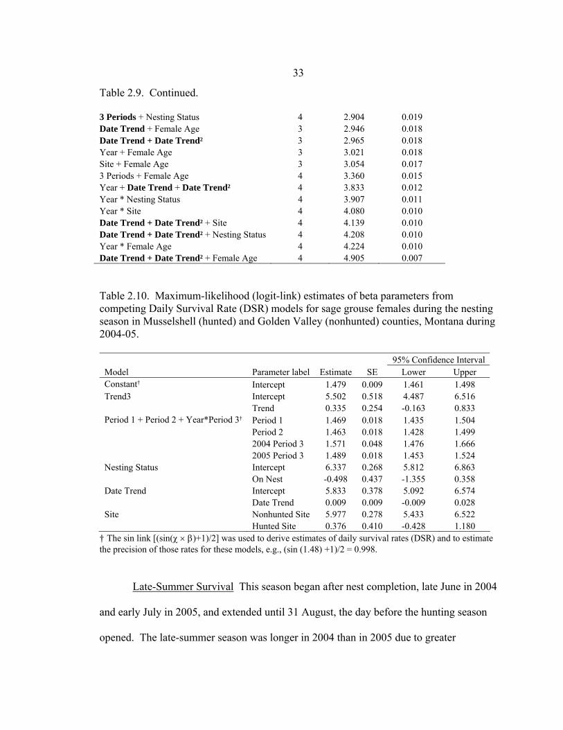
Table 2.9. Continued. 3 Periods + Nesting Status 4 2.904 0.019 Date Trend + Female Age 3 2.946 0.018 Date Trend + Date Trend² 3 2.965 0.018 Year + Female Age 3 3.021 0.018 Site + Female Age 3 3.054 0.017 3 Periods + Female Age 4 3.360 0.015 Year + Date Trend + Date Trend² 4 3.833 0.012 Year * Nesting Status 4 3.907 0.011 Year * Site 4 4.080 0.010 Date Trend + Date Trend² + Site 4 4.139 0.010 Date Trend + Date Trend² + Nesting Status 4 4.208 0.010 Year * Female Age 4 4.224 0.010 Date Trend + Date Trend² + Female Age 4 4.905 0.007

Table 2.10. Maximum-likelihood (logit-link) estimates of beta parameters from competing Daily Survival Rate (DSR) models for sage grouse females during the nesting season in Musselshell (hunted) and Golden Valley (nonhunted) counties, Montana during 2004-05.

95% Confidence Interval Model Parameter label Estimate SE Lower Upper Constant† Intercept 1.479 0.009 1.461 1.498 Trend3 Intercept 5.502 0.518 4.487 6.516 Trend 0.335 0.254 -0.163 0.833 Period 1 + Period 2 + Year*Period 3† Period 1 1.469 0.018 1.435 1.504 Period 2 1.463 0.018 1.428 1.499 2004 Period 3 1.571 0.048 1.476 1.666 2005 Period 3 1.489 0.018 1.453 1.524 Nesting Status Intercept 6.337 0.268 5.812 6.863 On Nest -0.498 0.437 -1.355 0.358 Date Trend Intercept 5.833 0.378 5.092 6.574 Date Trend 0.009 0.009 -0.009 0.028 Site Nonhunted Site 5.977 0.278 5.433 6.522 Hunted Site 0.376 0.410 -0.428 1.180

† The sin link [(sin(χ × β)+1)/2] was used to derive estimates of daily survival rates (DSR) and to estimate the precision of those rates for these models, e.g., (sin (1.48) +1)/2 = 0.998.

Late-Summer Survival This season began after nest completion, late June in 2004

and early July in 2005, and extended until 31 August, the day before the hunting season

opened. The late-summer season was longer in 2004 than in 2005 due to greater

34

renesting in 2005. I included 106 individuals in our analysis of female survival during

late summer, and 45 females were included in both years (Table 2.4). In 2004, one

female that was lost in July died between July and October, and was included as having

died during the late-summer season in our analyses. One radio-transmitter expired in late

summer in 2005.

The best model (ΔAICc = 0) provided support for our prediction that survival

would be higher in August 2004 than it would be in August 2005, when WNv was first

detected in sage grouse in our area (Table 2.11 and 2.12). The best model also estimated

a lower survival rate for females on the hunted site than on the nonhunted site (Table

2.12). The summed wi for models including Year*August was 0.54, whereas summed wi

for models including August, year, and site were 0.97, 0.61, and 0.30, respectively.

Models including female age, reproductive effort, and seasonal variation terms were not

supported.

Based on the estimated coefficients from the best model, survival estimates on

both sites were high and similar in July for both years, 0.99 (Table 2.13). However,

survival during August declined from 0.938 (SE = 0.037) in 2004 to 0.838 (SE = 0.054)

on the hunted site and from 0.978 (SE = 0.017) to 0.941 (SE = 0.035) on the nonhunted

site (Table 2.13).

35

Table 2.11. A priori models of Daily Survival Rate (DSR) for sage-grouse females during late summer in Musselshell (hunted) and Golden Valley (nonhunted) counties, Montana during 2004-05. Models were ranked by differences in AICc values, and the “*” symbol indicates an interaction between covariates. The Year * August term in bold type had the highest summed model weight.

Model # Parameters ΔAICc AICc weight Year * August + Site 4 0.000 0.164 August + Site 3 0.579 0.123 Year * August 3 1.107 0.094 August 2 1.830 0.066 Year + August 3 2.136 0.056 Year * August + Nest Fate 4 2.285 0.052 Year * August + Days Incubating 4 2.391 0.050 Year * August + August * SRE 4 2.784 0.041 Year * August + August * Days Rearing 4 3.015 0.036 Year * August + August * Brood Fate 4 3.081 0.035 Year * August + Female Age 4 3.089 0.035 Year * August + Days Laying 4 3.109 0.035 August + Days Laying 3 3.418 0.030 August + Nest Fate 3 3.521 0.028 August + Female Age 3 3.578 0.027 August + Days Incubating 3 3.728 0.025 August * Brood Fate 3 3.804 0.024 August * Days Rearing 3 3.831 0.024 August * SRE 3 3.831 0.024 Year * Site 4 7.880 0.003 Last 1/2 August + Site 3 8.314 0.003 Year + Site 3 8.496 0.002 Site 2 9.060 0.002 Year + Last 1/2 August 3 9.127 0.002 Year 2 9.377 0.002 Last 1/2 August 2 9.484 0.001 Constant 1 9.963 0.001 Year * Days Incubating + Site 5 10.363 0.001 Site + Nest Fate 3 10.549 0.001 Year + Nest Fate 3 10.706 0.001 Site + Days Laying 3 10.760 0.001 Site + Days Incubating 3 10.844 0.001 Year + Days Incubating 3 10.844 0.001 Site + Female Age 3 10.881 0.001 Last 1/2 August + Days Laying 3 10.921 0.001 Year * Days Incubating 4 11.019 0.001 Year * Nest Fate + Site 5 11.088 0.001 Last 1/2 August + Female Age 3 11.207 0.001 Last 1/2 August + Nest Fate 3 11.250 0.001 Days Laying 2 11.310 0.001 Year + Female Age 3 11.344 0.001

36

Table 2.11. Continued. Year + Days Laying 3 11.354 0.001 Last 1/2 August + Last 1/2 Aug * Days Rearing 3 11.368 0.001 Last 1/2 August + Days Incubating 3 11.432 0.001 Last 1/2 August + last 1/2 Aug * Brood Fate 3 11.446 0.001 Last 1/2 August + SRE 3 11.485 0.001 Female Age 2 11.691 0.000 Nest Fate 2 11.767 0.000 Days Incubating 2 11.932 0.000 Year * Nest Fate 4 12.189 0.000 Year * Days Laying + Site 5 12.299 0.000 Year * Days Incubating + Female Age 5 12.745 0.000 Year * Female Age 4 12.998 0.000 Year * Days Laying 4 13.042 0.000 Days Laying + Female Age 3 13.244 0.000 Nest Fate + Female Age 3 13.395 0.000 Days Incubating + Female Age 3 13.573 0.000 Year * Nest Fate + Female Age 5 13.985 0.000 Year * Days Laying + Female Age 5 15.020 0.000

Table 2.12. Covariate coefficient estimates, standard errors, and 95% confidence intervals for the best approximating model of late-summer survival of sage grouse females in Musselshell (hunted) and Golden Valley (nonhunted) counties, Montana during 2004-05. 95% Confidence Intervals

Parameter Estimate Std. error Lower Upper July 2004 & 2005 8.981 1.124 6.779 11.184 August 2004 -1.752 1.193 -4.091 0.587 August 2005 -2.773 1.050 -4.832 -0.715 Hunted site -1.074 0.659 -2.366 0.218 Table 2.13. Monthly survival estimates ±SE during late summer from the best approximating model for sage grouse females in Musselshell (hunted) and Golden Valley (nonhunted) counties, Montana during 2004-05. 95% Confidence Intervals

Month & Year(s) Study site Ŝ Std. error Lower Upper July 2004 & 2005 Hunted 0.989 0.011 0.968 1.0 July 2004 & 2005 Nonhunted 0.996 0.004 0.988 1.0 August 2004 Hunted 0.938 0.037 0.866 1.0 August 2004 Nonhunted 0.978 0.017 0.946 1.0 August 2005 Hunted 0.838 0.054 0.733 0.944 August 2005 Nonhunted 0.941 0.035 0.874 1.0

37

Discussion

My research documented differences in reproductive effort, renest survival, brood

survival, and reproductive success between a relatively dry year in 2004 and a relatively

wet year in 2005 (Appendix B). Increases in nesting and renesting probability, higher

survival of renests, and higher brood success may have been due to increased

precipitation and a subsequent increase in grass and forb abundance in 2005 (Woodward

2006). This increase may have provided better nutrition for females and chicks, better

cover at late-season nests, and better cover for chicks.

Reproductive Effort

Females initiated first nests between late March and early April, which was one to

three weeks earlier than initiation dates reported by other studies in Montana (Wallestad

1975, Moynahan et al. in press). Average clutch sizes were comparable to studies from

other parts of their range (see Schroeder et al. 1999 and Connelly et al. 2000 for review,

Moynahan et al. in press). Probabilities of nest initiation (0.72 to 1.0) and renest

initiation (0.0 to 0.63) were also within ranges recently reported for north-central

Montana (0.62 to 1.0 nesting probability and 0.0 to 0.56 renesting probability [Moynahan

et al. in press]). Renesting probabilities vary temporally and across the species range (5-

87% [see Schroeder et al. 1999 for review]), but few studies have reported renesting

probabilities higher than those reported here. In California, renesting probability was

reported as 63% (Popham and Gutiérrez 2003), and for north-central Washington

renesting was reported at 87% (Schroeder 1997). As in numerous other studies, I

38

documented higher nesting probability (Gregg 1991, Connelly et al. 1993, Holloran 2005,

Moynahan et al. in press) and higher renesting probability (see Schroeder et al. 1999 for

review, Gregg et al. 2006, Moynahan et al. in press) for adults than for yearlings.

Nest Survival

For both years combined, maximum-likelihood estimates of nest survival for a 28-

day incubation period were 0.32 for first nests and 0.56 for renests. This pattern, higher

survival estimates for renests than first nests, is consistent with numerous other studies

(Aldridge and Brigham 2001, Hall 2001, Moynahan et al. in press). If DSR during laying

is assumed to be the same as that for the incubation period, an assumption I was unable to

evaluate, the estimates from the best model would estimate nest survival for a 41-day

nesting period (13 days of egg laying [clutch size = 8] + 28 days of incubation) as 0.18

(SE = 0.04) for first nests and as 0.43 (SE = 0.09) for renests.

Nest survival estimates for a 28-day incubation period for north-central Montana

ranged from 0.24 to 0.32 for early-season nests and 0.28 to 0.42 for late-season nests

(Moynahan et al. in press). All other previously published studies reported apparent nest

success estimates, a method that is known to produce estimates that are biased high

(Mayfield 1961, 1975). Further, some of these studies utilized methods such as nest

searching to locate nests (e.g., Batterson and Morse 1948, Bean 1941, Keller et al. 1941,

Patterson 1952) rather than working with radio-marked females. Nest searching can

result in nest success estimates that are biased high if the sample of nests found is not

representative of the total population, e.g., if un-modeled heterogeneity among nest fates

exists, bias occurs because successful nests survive longer and are more likely to be

39

detected by investigators. Estimates from studies utilizing methods different from this

study ranged widely, from 15-86% (see Schroeder et al. 1999 for review, Aldridge and

Brigham 2001, Popham and Gutiérrez 2003, Holloran et al. 2005), and although they

overlap my estimates, they should not be directly compared with the maximum-

likelihood estimates obtained in this study. Excluding studies based on nest searching,

nest-success estimates ranged from 15-72%. Apparent nest success rates for this study

were 0.39 for first nests and 0.59 for renests, which were biased high by 22% (first nests)

and 5% (renests) compared to maximum-likelihood estimates. Moynahan et al. (in press)

also demonstrated that apparent nest success estimates could be biased high by 8% to

91% of the maximum-likelihood estimates. Due to the variability in bias of apparent nest

success estimates, future studies should utilize modern methods (e.g., maximum-

likelihood estimates) for analyzing nest-survival data so that estimates are more accurate

and comparisons can be made over time and between areas.

The survival of renests observed on our study is relatively high and may actually

be an underestimate given that some first nests were likely renests. Schroeder (1997)

suggested that as much as 29% of the nesting period (laying) is not monitored, because

most nests go undetected prior to incubation. However, the methods I used for

classifying nests as renests are similar to those used in other studies, and therefore,

estimates are comparable. Most renesting (38/41 renests) occurred in 2005, and high

renest survival relative to first nests may be attributable to both warmer temperatures

later in the nesting season in both years and to a bloom of yellow sweet clover (Melilotus

officinale) in 2005, an introduced biennial forb, that increased concealment around many

late-season nests (i.e., renests). Other Montana studies of greater sage-grouse (Moynahan

40

et al. in press) and plains sharp-tailed grouse (Tympanuchus phasianellus jamesi

[Bousquet 1996]) have also observed higher nest survival in years that coincided with

abundant yellow sweet clover.

Forb abundance may be a key factor influencing year-to-year variation in

reproductive effort and success. Forbs represent 18 to 50% of the diet of prelaying

females, increase the nutrient value of the diet in spring (Barnett and Crawford 1994),

and may be important for prelaying body condition (Barnett and Crawford 1994, Gregg et

al. 2006, Pyle and Crawford 1996). Gregg et al. (2006) documented higher plasma

protein in females that renested than those that did not, and in ruffed grouse (Bonasa

umbellus), increases in dietary protein increased clutch size, clutch mass, and chick

viability (Beckerton and Middleton 1982). Woodward (2006) documented a 2.5 fold

increase in forbs from 2004 to 2005 at this study area. Other studies have suggested a

similar relationship between forb availability and probability of renesting (Barnett and

Crawford 1994, Schroeder 1997). I suspect that a higher proportion of forbs comprised

the diets of prelaying females in 2005, the year with higher nesting and renesting

probabilities, and that this increase in reproductive effort was probably due to better

nutritional condition of females.

Land-management practices that maintain forb availability and abundance may be

critical for stabilizing or increasing production. Further, it would be useful to know

which other factors encourage females to invest in reproduction. Reproductive effort

may be influenced not only by forb abundance and female age or experience but could

also be influenced by investment in reproduction in the preceding year or snow depth

during winter.

41

Brood Survival

Point estimates of brood survival to 30-days post-hatch were higher in 2004

(71%) than in 2005 (84%), but estimates were too imprecise to allow confidence in

measures of annual variation. Brood survival for both years combined was 79%. These

brood-survival estimates suggest less annual variation than estimates published

elsewhere. These estimates were within the range reported for north-central Montana

(21-76% [Moynahan 2005]) and were similar to apparent brood-survival estimates

reported for a study conducted adjacent to our area thirty years prior to this study (44-

77% [Wallestad 1975]). The brood-survival estimates I observed were higher than

estimates for Washington (0.36 to 0.52 [Sveum 1995]), but were within the range of

estimates for Wyoming, (0.33 to 1.0 [Heath et al. 1998, Holloran 2005, Slater 2003]), but

these studies used a different period length for calculating brood survival. However, two

features are noteworthy: 1) most chicks die early in brood-rearing and so estimates from

periods of different lengths may provide more reasonable comparisons than might be

expected if survival were not high and relatively constant after the first few weeks of the

brood-rearing period, and 2) I visited females at night to determine whether or not they

had broods, which improved our brood-detection probability. Thus, except for a study in

Alberta that reported 0.63 brood survival to 30 days post-hatch for radio-marked chicks

(Aldridge 2005), reports from other studies are likely underestimates of brood survival.

Chick survival is thought to be limiting population growth in Alberta, but the estimates in

my study are higher than those of Aldridge (2005) which suggests that brood-rearing

conditions are more favorable in central Montana. The increase in brood survival that I

42

observed from 2004 to 2005 may have been attributable to the increase in grass and forbs,

including the bloom of yellow sweet clover, which provided better cover and food

availability for chicks. This annual variation may also have been related to changes in

insect abundance.

Due to low probability of detecting all chicks, I was not able to estimate chick

survival, which makes drawing conclusions about productivity difficult. Brood survival

estimates provide crude estimates of actual chick survival. Brood survival overestimates

chick survival (Aldridge 2005), and therefore, brood-survival estimates must be viewed

cautiously as measures of productivity. However, obtaining reliable estimates of chick

survival will require new technology, innovative observation methods, or evidence that

radio-marking chicks at hatch does not affect their survival. Because most hens with

chicks tend not to flush at night, even with investigators approaching to within ≤10 m, the

risk of increased mortality due to nighttime disturbance is low. I expect chick survival to

continue to be a difficult parameter to estimate. Researchers should estimate chick

survival by counting chicks at night to increase detectability, and conducting multiple

counts to allow estimation of detection probability. In this way, more accurate estimates

of both chick survival and production could be obtained. We may then be able to learn

more about timing and causes of chick mortality and more accurately model sage grouse

population dynamics and estimate population growth.

Because renests had a higher probability of success than first nests, and most

renests occurred in 2005, and because brood survival may have been slightly higher in

2005, reproductive success was 50% greater in 2005 (0.43) than in 2004 (0.28). I report

reproductive success as the proportion of females that successfully raised a brood to 30

43

days old. Reproductive success was previously reported at 50% for a Washington study,

a study that also observed extremely high renesting probabilities (0.87 [Schroeder 1997]).

Typically, studies have reported “reproductive success” as the proportion of females that

successfully hatch at least one chick, which has ranged from 15% to 70% (see Schroeder

et al. 1999 for review) and during this study, was 39% in 2004 and 50% in 2005.

Female Survival

Few published studies of sage-grouse females report seasonal-survival estimates

(Connelly et al. 2004); most report annual estimates. Some report survival from spring

through fall or suggest that overwinter survival is high (Robertson 1991, Wik 2002,

Hausleitner 2003, Zablan 2003). More studies are needed that evaluate seasonal

differences in survival. Where available, I discuss our seasonal estimates in relation to

other studies. I discuss the results of this study in relation to annual estimates from other

studies in Chapter 3.

Nesting-Season Survival Our results indicate that female survival during the

nesting seasons was constant across all covariate conditions. The constant-survival

model estimated monthly female survival rate as 0.94, which was near the high end of the

range of estimates reported for north-central Montana during the nesting season (0.75 to

0.99 [Moynahan et al. 2006]) and was within the range of estimates for a recent study in

Colorado (0.91 to 0.99 [Hausleitner 2003]). I did not observe age-specific variation in

female survival. However, there was considerable model selection uncertainty, and

models including both within and among year variation, site, and nesting status received

some support. Although I discuss each of these effects with regard to our predictions

44

below, I cannot make strong inferences about these effects due to model-selection

uncertainty and lack of precision in these estimates.

Within-season variation was supported in the second and third best models. The

trend model, which allowed survival to differ across the season as an increasing or

decreasing trend, indicated that survival may have increased steadily across the season.

The period model, which allowed survival to differ among three different portions of the

season and to vary between years during the third period, indicated that survival may

have been similar in the first two periods of both years and increased more in the third

period during 2004 than in 2005. Biologically, the last period represented different

female activity between years. Because renest initiation was low in 2004, the last period

was shorter and few females incubated nests far into the last period (n = 4). In 2005,

because renesting was high, the last period was 17 days longer and many females were

still incubating renests during the late period (n = 30). This within- and among-year

variation in survival during the nesting season may represent differences in survival for

females on early versus late-season nests (first nests versus renests) or differences in

survival between nesting and non-nesting females. Increased cover at nest sites later in

the season may decrease probability of detection by predators and increase a female’s

probability of survival, or females with low quality nest sites may be detected by

predators earlier and the remaining females would be those at better nest sites conferring

higher probability of female survival.

As predicted, my results suggest that survival was lower for female sage grouse

while incubating nests than while off nests. A model including nesting status received

some support from the data. Additionally, a model including the year * period 3 term,

45

which supported lowered survival during the last period of the nesting season in 2005

than in 2004, may also lend support to this prediction. More females were still

incubating nests during the last period in 2005 than in 2004, and female survival was

lower during the last period in 2005 than in 2004.

This finding, that females have lower survival while incubating, contrasts with

those of a recent study in north-central Montana, in which nesting females were reported

to have higher survival than non-nesting females (Moynahan et al. 2006). However,

while nesting status of females was used to address the same prediction, nesting status

was represented differently in my analysis than in Moynahan et al. (2006). I included the

term for each day of the nesting season (nesting status: 0 = off nest, 1 = on nest) for each

female to evaluate the risk of incubating a nest. In the north-central Montana study,

nesting status defined nesting females as those for which a nest was detected and non-

nesting females were defined as those for which no nest was detected (0 = no nest

detected, 1 = nest detected) and was used to evaluate the same risk. This pattern may be

misleading in three ways. First, females may die before their nests are detected and

would therefore go undetected as nesting females. Second, the timing of death, if early in

the season, reduces the probability of finding a female on a nest. Third, as pointed out by

Moynahan et al. (2006), with the covariate constructed as nesters versus non-nesters, it

may better reflect a difference, such as body condition, between females that choose to

nest and those that do not, rather than the risk associated with incubating a nest. When I

included the same categorical variable of whether or not a female was detected on a nest,

the results were the same as Moynahan et al. (2006), and a model with only this term was

the best supported in that model set. However, during my study, I did not detect a nest

46

for 20 females, and of those 20, five died. But, all five either died within the first two to

three weeks of the nesting season, and they may have been nesting but nests went

undetected, and they were not as likely to be detected on a nest compared to other

females, given timing of death.

During the nesting season, female survival was lower on the nonhunted site, 80%,

than on the hunted site, 86%, but the estimates were too imprecise to allow us to be very

confident of the exact level of site variation. Although this site difference is consistent

with the hypothesis for compensation for the effect of hunting (higher survival of birds at

reduced breeding densities [Nichols et al. 1984]), I did not collect data on bird densities.

It is more likely that this difference in female survival between sites was due to factors

unrelated to hunting, such as differences in habitat quality or predator communities

between sites.

Late-Summer Survival In contrast to the nesting season, survival was lower on

the hunted site than on the nonhunted site later in the summer. Differences in female

survival between sites during this season may also be due to landscape-scale factors, such

as differences in the quality of sagebrush habitat or predator communities between sites.

West Nile virus was first detected in sage grouse in summer 2003 in both north-central

and southeastern Montana but was not detected in this study area in central Montana until

August 2005. West Nile virus was likely a major contributor to the decrease in survival

observed in this study between August 2004 (0.94 to 0.98) and August 2005 (0.84 to

0.94). The range of monthly survival estimates for July and August (0.84 to nearly 1.0)

in this study was wider and lower than estimates reported for north-central Montana for

47

the same time period (0.92 to 0.97 [Moynahan et al. 2006]), but the range was not as low

or wide as estimates reported for southeastern Montana (0.45 to 0.89 [Naugle et al.

2004]). It is important to continue to monitor the prevalence and effects of WNv on sage

grouse.

West Nile virus was only detected in three out of eight testable samples in 2005,

which included one unmarked female, and in 2004 tests of remains from three females

were negative. Infection with WNv has resulted in 100% mortality in laboratory studies

of sage grouse (Clark et al. 2006). Most of the remains that were tested from this study

only included bone fragments or molting feathers, which are not ideal for WNv screening

(Walker et al. 2004), and infection and mortality due to WNv may have been higher than

detected in 2005 or may have gone undetected in this area in 2004. Precipitation was

greater in 2005 than 2004, which may have contributed to increased mosquito production

and higher infection rates that may have subsequently increased our probability of

detecting WNv in 2005. Alternatively or additionally, heat stress during late summer,

reductions in availability of water, or the timing of molt may have also contributed to the

decrease in survival during August.

Future Research

Central Montana represents some of the most intact, contiguous sagebrush habitat

within current greater sage-grouse range in Montana (Montana Sage Grouse Working

Group 2005), and like Wyoming, Idaho, Nevada, and Oregon, Montana supports

relatively abundant numbers of sage grouse compared to the rest of their range (Connelly

et al. 2004). Currently, no published population model exists for integrating such a

48

combination of vital rates together in a way that allows me to estimate population growth

rate. But, lek counts do suggest that the rates are such that large numbers are being

sustained (Appendix C). Of course, available data do not allow me to consider the

possible role of immigration in the population’s dynamics, and data on exchange of

individuals with surrounding populations would also be useful.

Variation in reproductive effort and success and high survival of renests has

important implications for management. Managing sagebrush habitats to maintain forb

availability and abundance may be critical for stabilizing or increasing production.

However, variation in reproductive effort and success if accompanied by negatively

covarying female survival may stabilize population growth. If there is a reproductive

cost to survival, then the age structure of females in the population may be different

during a spring following a year of high reproductive investment. Adult females are

important to the population, because they are more likely to nest and renest. Therefore,

reproductive success may be lower during a spring following a year of high reproductive

investment. The cost of reproduction to female survival immediately following the

breeding season is considered in the Chapter 3. In future studies, it would be helpful to

consider how investment in reproduction affects future fecundity and survival. Future

studies should also directly assess how habitat characteristics influence reproductive

effort, nest survival, brood survival, and female survival; this may be the subject of a

collaborative effort between my project and the habitat projects conducted in conjunction

with my project in the near future.

49

Literature Cited

Aldridge C. L. and R. M. Brigham. 2001. Nesting and reproductive activities of greater

sage-grouse in a declining northern fringe population. The Condor 103:537-543.

Aldridge, C. L. 2005. Identifying habitats for persistence of greater sage-grouse (Centrocercus urophasianus) in Alberta, Canada. Dissertation, University of Alberta, Edmonton, Alberta, Canada.

Armstrup, S. C. 1980. A radio-collar for game birds. Journal of Wildlife Management 44:214-217.

Barnett, J. K. and J. A. Crawford. 1994. Pre-laying nutrition of sage grouse hens in Oregon. Journal of Range Management 47:114-118.

Batterson, W. M. and W. B. Morse. 1948. Oregon Sage Grouse. Oregon Game Commission, Oregon Fauna Service 1, Portland, Oregon USA.

Bean, R. W. 1941. Life history studies of the sage grouse (Centrocercus urophasianus) in Clark County, Idaho. Thesis, Utah State Agricultural College, Logan, Utah, USA.

Beckerton, P. R. and A. L. A. Middleton. 1982. Effects of dietary protein levels on ruffed grouse reproduction. Journal of Wildlife Management. 46:569-579.

Bergerud A.T. 1988. Population ecology of North American grouse. Pages 578-648 in Adaptive strategies and population ecology of northern grouse. A.T. Bergerud and M.W. Gratson, editors. University of Minnesota Press, Minneapolis, Minnesota.

Bergerud, A. T. and M. W. Gratson. 1988. Survival and breeding strategies of grouse. Pages 473-577 in Adaptive strategies and population ecology of northern grouse. A. T. Bergerud and M.W. Gratson, editors. University of Minnesota Press, Minneapolis, Minnesota.

Bousquet, K. R. 1996. Habitat preferences of sharp-tailed grouse broods on the Charles M. Russell National Wildlife Refuge. Thesis. Montana State University, Bozeman, Montana, USA.

Brinkman, T.J., C.S. DePerno, J.A. Jenks, J.D. Erb, B.S. Haroldson. 2002. A vehicle-mounted radiotelemetry design. Wildlife Society Bulletin 30:256-258.

Burnham, K.P., and Anderson, D. R. 2002. Model selection and multi-model inference: a practical information theoretic approach. Second edition. Springer-Verlag Inc., New York, USA.

50

Clark, L., J. Hall, R. McLean, M. Dunbar, K. Klenk, R. Bowen, C. A. Smeraskiz. 2006. Susceptibility of greater sage-grouse to experimental infection with West Nile virus. Journal of Infectious Diseases 42:96-105.

Connelly, J. W., R. A. Fischer, A. D. Apa, K. P. Reese, W. L. Wakkinen. 1993. Renesting by sage grouse in southeastern Idaho. The Condor 95:1041-1043.

Connelly, J.W. and C.E. Braun. 1997. Long-term changes in Sage Grouse Centrocercus urophasianus populations in western North America. Wildlife Biology 3:229-234.

Connelly, J. W., M.A. Schroder, A R. Sands, and C. E. Braun. 2000. Guidelines to manage sage grouse populations and their habitats. Wildlife Society Bulletin 28: 967-985.

Connelly, J. W., S. T. Knick, M. A. Schroeder, and S. J. Stiver. 2004. Conservation Assessment of Greater Sage-grouse and Sagebrush Habitats. Western Association of Fish and Wildlife Agencies. Unpublished Report. Cheyenne, Wyoming.

Cox, R. R., J. D. Schaff, B. E. Jamison and R. S. Lutz. 2002. Using an electronic compass to determine telemetry azimuths. Wildlife Society Bulletin 30:1039-1043.

Crawford, J. A., and R. S. Lutz.1985. Sage grouse population trends in Oregon, 1941–1983. The Murrelet 66:69-74.

Crunden, C. W. 1963. Age and sex of grouse from wings. Journal of Wildlife Management 27:846-849.

Eng, R. L. 1955. A method for obtaining Sage Grouse age and sex ratios from wings. Journal of Wildlife Management 19:267-272.

Eng, R. L. and P. Schladweiler. 1972. Sage grouse winter movements and habitat use in central Montana. Journal of Wildlife Management 36: 141-146.

Geisen, K. M., T. J. Schoenberg, and C. E. Braun. 1982. Methods for trapping Sage Grouse in Colorado. Wildlife Society Bulletin 10:224-231.

Gregg, M. A. 1991. Use and selection of nesting habitat by sage grouse in Oregon. Thesis. Oregon State University, Corvallis, Oregon, USA.

Gregg, M. A., M. R. Dunbar, J. A. Crawford, and M. D. Pope. 2006. Total plasma protein and renesting by greater sage-grouse. Journal of Wildlife Management 70:472-478.

Hall, F. J. 2001. Learning the secrets of Sage Grouse. Pages 8-9 in California Department of Fish and Game Publication. Tracks, Issue 25.

51

Hausleitner, D. 2003. Population dynamics, habitat use and movements of Greater Sage-grouse in Moffat County, Colorado. M. S. Thesis, University of Idaho, Moscow, Idaho, USA.

Heath, B. J., R. Straw, S. H. Anderson, J. Lawson, and M. Holloran. 1998. Sage-grouse productivity, survival, and seasonal habitat use among three ranches with different livestock grazing, predator control, and harvest management practices. Wyoming Game and Fish Department Completion Report, Rawlins, Wyoming. 66 pp.

Holloran, M. J. 2005. Greater sage-grouse (Centrocercus urophasianus) population response to natural gas field development in western Wyoming. Dissertation, University of Wyoming, Laramie, Wyoming, USA.

Holloran, M. J., B. J. Heath, A. G. Lyon, S. J. Slater, J. L. Kuipers, S. H. Anderson. 2005. Greater sage-grouse nesting habitat selection and success in Wyoming. Journal of Wildlife Management 69:638-649.

Hornaday, W. T. 1916. Save the sage grouse from extinction, a demand from civilization to the western states. New York Zoological Park Bulletin 5:179-219.

Huwer, S. L. 2004. Evaluating greater sage-grouse brood habitat using human-imprinted chicks. Thesis, Colorado State University, Fort Collins, Colorado, USA.

Keller, R. J., H. R. Shepard, and R. N. Randall. 1941. Survey of 1941: North Park, Jackson County, Moffat County, including comparative data of previous season. Sage Grouse Survey 3. Colorado Game and Fish Commission, Denver, Colorado USA.

Klett, A. T., and D. H. Johnson. 1982. Variability in nest survival rates and implications to nesting studies. Auk 99:77-87.

Lane, V. R. 2005. Sage-grouse (Centrocercus urophasianus) nesting and brood-rearing sagebrush habitat characteristics in Montana and Wyoming. Thesis, Montana State University, Bozeman, Montana, USA.

Mayfield, H. R. 1961. Nesting success calculated from exposure. Wilson Bulletin 73:255-261.

Mayfield, H. R. 1975. Suggestions for calculating nest success. Wilson Bulletin 87:456-466.

Montana Sage Grouse Work Group. 2005. Management plan and conservation strategies for sage grouse in Montana – final. Montana, Fish, Wildlife, Parks, USA.

52

Moynahan, B. J. 2005. Landscape-scale factors affecting population dynamics of greater sage-grouse (Centrocercus urophasianus) in north-central Montana, 2001-2004. Dissertation, University of Montana, Missoula, Montana, USA.

Moynahan, B. J., M. S. Lindberg, and J. W. Thomas. 2006. Factors contributing to process variance in annual survival of female greater sage-grouse in north-central Montana. Ecological Applications 16:1529-1538.

Moynahan, B. J., M. S. Lindberg, J. J. Rotella, J. W. Thomas. In Press. Factors affecting nest survival of greater –sage-grouse in northcentral Montana. Journal of Wildlife Management.

National Oceanic and Atmospheric Administration. 2006. Annual climatological summary, Roundup, Montana. Available at: http://cdo.ncdc.noaa.gov/ancsum/ACS. Accessed August 3, 2006.

Naugle, D. E., C. L. Aldridge, B. L. Walker, T. E. Cornish, B. J. Moynahan, M. J. Holloran, K. Brown, G. D. Johnson, E. T. Schmidtmann, R. T. Mayer, C. Y. Kato, M. T. Matchett, T. J. Christiansen, W. E. Cook, T. Creekmore, R. D., Falise, E. T. Rinkes, and M. S. Boyce. 2004. West Nile virus: a pending crisis for greater sage-grouse. Ecology Letters 7:704-713.

Naugle, D. E. C. L. Aldridge, B. L. Walker, K. E. Doherty, M. R. Matchett, J. McIntosh, T. E. Cornish, and M. S. Boyce. 2005. West Nile virus and sage-grouse: What more have we learned? Wildlife Society Bulletin 33:616–623.

Nichols, J. D., M. J. Conroy, D. R. Anderson, and K. P. Burnham. 1984. Compensatory mortality in waterfowl populations: a review of the evidence and implications for research and management. Transactions of the North American Wildlife and Natural Resources Conference 49:535-554.

Patterson, R. L. 1952. Sage Grouse hunting seasons. Wyoming Wildlife 16:10-13.

Popham, G. P. and R. J. Gutiérrez. 2003. Greater sage-grouse Centrocercus urophasianus nesting success and habitat use in northeastern California. Wildlife Biology 9:327-334.

Pyle, W.H. and J.A. Crawford. 1996. Availability of foods of sage grouse chicks following prescribed burning in sagebrush-bitterbrush. Journal of Range Management 49:320–324.

R Development Core Team. 2006. R: A language and environment for statistical computing. R Foundation for Statistical Computing, Vienna, Austria. ISBN 3-900051-07-0, URL http://www.R-project.org.

53

Robertson, M. D. 1991. Winter ecology of migratory sage grouse and associated effects of prescribed fire in southeastern Idaho. M.S. Thesis, University of Idaho, Moscow, Idaho, USA.

Rotella, J. J., R. G. Clark, and A. D. Afton. 2003. Survival of female scaup: effects of body size, age, and reproductive effort. The Condor 105:336-347.

Ruf, T., J. Fietz, W. Schlund, and C. Bieber. 2006. High survival in poor years: life-history tactics adapted to mast seeding in the edible dormouse. Ecology 87:372-381.

Sæther, B. and O. Bakke. 2000. Avian life-history variation and contribution of demographic traits to the population growth rate. Ecology 81:642-653.

Samuel, M. D. and M. R. Fuller. 1996. Wildlife radiotelemetry. Pages 370-418 in T. A. Bookhout, editor. Research and management techniques for wildlife and habitats. Fifth edition. The Wildlife Society, Bethesda, Maryland, USA.

Sandercock, B. K., K. Martin, S. J. Hannon. 2005. Life history strategies in extreme environments: comparative demography of arctic and alpine ptarmigan. Ecology 86:2173-2186.

Schroeder, M. A. 1997. Unusually high reproductive effort by sage grouse in a fragmented habitat in north-central Washington. The Condor 99:933-941.

Schroeder, M. A., J. R. Young, and C. E. Braun. 1999. Sage grouse (Centrocercus urophasianus). Pages 1-28 in A. Poole and F. Gill, editors. The Birds of North America, Number 425. The Birds of North America, Inc., Philadelphia, Pennsylvania, USA.

Schroeder, M. A., C. L. Aldridge, A. D. Apa, J. R. Bohne, C. E. Braun, S. D. Bunnell, J. W. Connelly, P. A. Deibert, S. C. Gardner, M. A. Hilliard, G. D. Kobriger, S. M. McAdam, C. W. McCarthy, J. J. McCarthy, D. L. Michell, E. V. Rickerson and S. J. Stiver. 2004. Distribution of sage-grouse in North America. The Condor 106:363-376.

Seber, G. A. F. 1982. The estimation of animal abundance and related parameters. Second edition. Macmillian, New York, New York, USA.

Slater, S. J. 2003. Sage-grouse (Centrocercus urophasianus) use of different-aged burns and the effects of coyote control in southwestern Wyoming. Thesis, University of Wyoming, Laramie, Wyoming, USA.

Sveum, C. M. 1995. Habitat selection by sage grouse hens during the breeding season in south-central Washington. Thesis, Oregon State University, Corvalis, Oregon, USA.

54

U.S. Fish and Wildlife Service. 2004. 30-day finding for petitions to list the greater sage-grouse as threatened or endangered. Federal Registry 69(77):21484-21494.

Wakkinen, W.L., K.P. Reese, J.W. Connelly, R.A. Fischer. 1992. An improved spotlighting technique for capturing sage grouse. Wildlife Society Bulletin 20:425-426.

Walker, B. L., D. E. Naugle, K. E. Doherty, and T. E. Cornish. 2004. Outbreak of West Nile virus in greater sage-grouse and guidelines for monitoring, handling, and submitting dead birds. Wildlife Society Bulletin 32: 1000–1006.

Wallestad, R. and D. Pyrah. 1974. Movement and nesting of sage grouse hens in central Montana. Journal of Wildlife Management. 38:630-633.

Wallestad, R. and P. Schladweiler. 1974. Breeding season movements and habitat selection of male sage grouse. Journal of Wildlife Management 38:634-637.

Wallestad, R. 1975. Montana sage grouse. Montana Department of Fish and Game and United States Bureau of Land Management, address, Montana, USA.

Westerkov, K. 1950. Methods for determining the age of game bird eggs. Journal of Wildlife Management 14(1):56-67.

White, G. C. and R. A. Garrott. 1990. Analysis of wildlife radio-tracking data. Academic Press, London, United Kingdom.

White, G. C. and K. P. Burnham. 1999. Program MARK: survival estimation from populations of marked animals. Bird Study (Supplement) 46.

Wik, P. 2002. Ecology of greater sage-grouse in south-central Owyhee County, Idaho. Thesis, University of Idaho, Moscow, Idaho, USA.

Woodward, J. K. 2006. Greater sage-grouse (Centrocercus urophasianus) habitat in central Montana. Thesis, Montana State University, Bozeman, Montana, USA.

Zablan, M. A., C. E. Braun, and G. C. White. 2003. Estimation of greater sage-grouse survival in North Park, Colorado. Journal of Wildlife Management 67:144-154.

Zhou, S. 2002. Estimating parameters of derived random variables: comparison of the delta and parametric bootstrap methods. Transactions of the American Fisheries Society 131:667-675.

55

CHAPTER THREE.

FALL AND WINTER SURVIVAL RATES AND CAUSES OF MORTALITY AMONG HUNTED AND NONHUNTED GREATER SAGE-GROUSE

IN CENTRAL MONTANA

Introduction

Greater sage-grouse (Centrocercus urophasianus, hereafter sage grouse)

populations have been declining throughout their historical range in western North

America since the early 1900s (Hornaday 1916), with current abundance estimated at 1-

31% of the numbers present prior to European settlement in the 1800s (United States Fish

and Wildlife Service 2004). In addition to a dramatic decline in abundance, sage grouse

distribution has contracted by as much as 44% (Schroeder et al. 2004). Historically, the

largest populations existed in Colorado, Idaho, Oregon, Wyoming, and Montana

(Connelly and Braun 1997). Much of central Montana is still in relatively contiguous

sagebrush-steppe habitat, supports relatively large numbers of sage grouse, and supports

populations that appear to be relatively stable (Connelly et al. 2004, Montana Sage

Grouse Work Group 2005).

There are a number of possible factors contributing to sage grouse population

declines, including energy development (see Connelly et al. 2000a for review, Holloran

2005), West Nile virus (Naugle et al. 2004), weather (Connelly and Braun 1997,

Connelly et al. 2000a, Moynahan et al. 2006), predation (Batterson and Morse 1948),

habitat alteration (natural and human-caused), pesticide and herbicide use, and harvest

(see Connelly and Braun 1997, Schroeder et al. 1999, and Connelly et al. 2000a for

56

review). Despite increasing concerns, sage grouse are still legally harvested in most of

their current range, including Montana. Direct investigation of how harvest affects

population vital rates and population growth, and the magnitude of harvest effects

relative to other sources of mortality, is needed for informed management of harvested

species (Nichols and Johnson 1989), especially species that are declining. Further,

because harvest is regulated by state governments, it is a valuable management action

that can be directly manipulated.

The realized effect of harvest on natural mortality and population growth for a

given species depends on the magnitude and timing of density-dependent natural

mortality and the existence of reproductive compensation (Nichols et al. 1984). If

harvest reduces densities, survival probability may increase for the remaining individuals

after harvest if density-dependent mortality occurs at some time later in the annual cycle.

A subsequent reduction in nonhunting density-dependent mortality may directly

compensate for at least part of the hunting loss. Alternatively, if hunting reduces

densities below some biological threshold level necessary for survival (inverse density

dependence), survival probability may decrease for the remaining individuals

(Courchamp et al. 1999). If harvest reduces breeding densities and a population has

density-dependent reproduction, then indirect compensation may occur through increases

in reproductive success or recruitment. The management question becomes, at different

levels of harvest and at varying population densities, what is a population’s demographic

response? Ideally, this question would be addressed by applying a range of harvest levels

randomly to multiple, replicated sites with varying population densities and habitat

qualities and by conducting investigations at landscape scales adequate to detect

57

dispersal. However, assessing population responses across densities for diverse harvest

levels is often prohibitively difficult, and many studies have relied on a variety of

constrained research designs, including comparing fall population numbers to spring

breeding numbers, comparing fall numbers to annual mortality rates, evaluating the

magnitude of harvest mortality relative to other sources of mortality, comparing annual

survival rates and kill rates, and comparing survival between hunted and nonhunted

populations.

Several investigations of harvest effects in upland game birds have compared

survival rates and causes of mortality between hunted and nonhunted radio-marked

populations (Smith and Willebrand 1999, Pedersen et al. 2003, McAuley et al. 2005). In

two studies of willow ptarmigan, no evidence or weak evidence for compensation was

found, but those populations did not decline (Smith and Willebrand 1999, Pedersen et al.

2003). Stable population size in those studies was attributed to immigration of juveniles,

not compensation, and suggested that as the study area expanded evidence for

compensation would grow weaker (Smith and Willebrand 1999, Pedersen et al. 2003). In

woodcock, 36% of the total mortality was attributed to hunting, and researchers

concluded that harvest was not reducing survival (McAuley et al. 2005).

Uncertainty about how harvest impacts sage grouse vital rates remains. Thus far,

published research investigating the effects of harvest on sage grouse vital rates has

suggested that harvest mortality may not be compensatory (Johnson and Braun 1999,

Connelly et al. 2000b, Connelly et al. 2003) or in contrast, has reported that hunting has

little impact on populations (Wallestad 1975, Crawford 1982, Braun and Beck 1985).

Because population size or density may influence survival (Anderson and Burnham 1976,

58

Caswell et al. 1985, Nichols et al. 1984, Krementz et al. 1988, Nichols and Johnson 1989,

Sedinger and Rextad 1994, Sedinger and Rotella 2005), it is sometimes difficult to draw

strong conclusions about the effects of hunting with some study designs. For example, a

major limitation of some harvest studies in both waterfowl and upland game birds has

been the historical pattern of manipulating harvest regulations in response to changes in

population size which makes it difficult to ascertain the effect on survival (Anderson and

Burnham 1976, Caswell et al. 1985, Krementz et al. 1988). Further, some study designs

have led to divergent interpretation of results (Connelly et al. 2003, Reese et al. 2005,

Sedinger and Rotella 2005). Harvest may impact sage grouse populations very

differently across their range, and thus, area-specific data on the impact of harvest, and

the magnitude of this impact relative to other potential sources of mortality, are necessary

for informed management.

Other factors influence mortality. Greater reproductive effort (i.e., renesting or

days brood rearing) may reduce probability of survival or overall fecundity (this trade-off

is the cost of reproduction) as documented in long-lived sea birds in variable and harsh

environments (Reid 1987, Jacobsen et al. 1995, Erikstad et al. 1997, 1998, Golet et al.

1998). Previous research has suggested this cost of reproduction may also exist for sage

grouse (Bergerud and Gratson 1988, Moynahan et al. 2006). Age-specific variation in

survival (Zablan et al. 2003) and age-specific reproductive success have been previously

documented in sage grouse (Schroeder et al. 1999). Habitat alteration and fragmentation

are thought to be the leading cause of decline in abundance and distribution (see Connelly

and Braun 1997, Schroeder et al. 1999, and Connelly et al. 2000a for review), and

drought may also affect populations (Connelly and Braun 1997, Connelly et al. 2000a,

59

Moynahan et al. 2006). Differences in predator communities may also impact survival

(Connelly et al. 2000a). Severe winter weather (Moynahan et al. 2006) and West Nile

virus (WNv [Naugle et al. 2004, Walker et al. 2004, Naugle et al. 2005, Moynahan et al.

2006]) have recently been documented to negatively affect survival. Harvest theory

indicates that direct compensation should occur following harvest, therefore it is

necessary to consider survival during winter.

Due to uncertainty about the impact of harvest on vital rates and uncertainty about

the relative importance of harvest compared to other sources of mortality, we designed a

case study with the following objectives: 1) simultaneously compare survival rates during

the hunting season and overwinter between adjacent hunted and nonhunted sites with

similar landscape and population characteristics, 2) evaluate nonhunting factors

influencing survival during the hunting season, 3) assess the relative importance of

different mortality factors on sage grouse overwinter, and 4) assess, to the extent

possible, the importance of harvest to the sage grouse populations studied and to make

recommendations for future investigations about the effects of harvest on sage grouse.

Study Area

I studied sage grouse within approximately 3,000 km2 in Musselshell and Golden

Valley Counties in central Montana from 2003-2005 (46° 26´ to 46° 76´ N, 108° 32´ to

109 15´ W) (Appendix A1). This area was primarily sagebrush-steppe (80%)

interspersed with native prairie grasslands (<1%), ponderosa pine (<1%), and both dry

and irrigated agriculture (14%) (Appendix A2). Soil taxonomy is described in detail by

Woodward (2006). Wyoming big sagebrush (Artemisia tridentata wyomingensis),

60

western wheatgrass (Agropyron smithii), green needlegrass (Stipa viridula), and blue

grama (Bouteloua gracilis) characterized the predominant habitat and cover type. Two

habitat types dominated lowlands: 1) plains silver sagebrush (A. cana cana) with western

wheatgrass and 2) greasewood (Sarcobatus vermiculatus) with Gardner saltbrush

(Atriplex gardneri), inland saltgrass (Distichlis spicata), and green needlegrass.

Historical and current land uses include cattle and sheep grazing. Relatively little energy

development (i.e., oil or gas) occurred within the core areas of the study sites. Portions of

land continued to be converted to dry and irrigated cropland, including enrollment in the

federal Conservation Reserve Program (CRP), and land was treated to remove sagebrush.

The 70-year precipitation average was 37 cm, but severe to extreme drought conditions

persisted from 2000-2005 (Appendix B). Annual precipitation was 25 cm in 2004 and 46

in 2005, and average monthly temperature ranged from -7°C in January to 22°C in July

(National Oceanic and Atmospheric Administration [NOAA] 2006). Elevation ranged

from 800 to 1,500 m. The study area supported relatively abundant breeding populations

of nonmigratory sage grouse. Peak attendance at 25 leks averaged 24 to 37 males per lek

(range 5-76 males among 25 leks) from 2002-2005 (Appendix C, Montana Fish, Wildlife

and Parks [FWP], unpublished data). A large proportion of land in this region was

enrolled in FWP’s Block Management Program, which facilitates hunting access on

private lands, and the FWP Commission had the ability to close a large area to sage

grouse hunting to conduct this study.

I defined one hunted site and one nonhunted site within the study area by trapping

birds at four (nonhunted) to five (hunted) adjacent leks that collectively had high male

attendance. About 40% of the hunted site was a sagebrush cover type, similar to the

61

nonhunted site, and about 10% of the hunted site was converted to some type of

agriculture which was slightly higher than the nonhunted site, 4% (Appendix A2). I

expected that most birds would remain within 5 km of the leks where they were trapped

(Eng and Schladweiler 1972, Wallestad and Pyrah 1974, Wallestad and Schladweiler

1974, Wallestad 1975). Thus, for vegetation sampling and site descriptions, I defined

each study site as a “lek complex,” the area within overlapping 5-km-radii around trapped

leks (Appendix A1).

The hunted site was 287 km2 in area, of which 60% was privately owned, and

40% was publicly owned and managed by either the Bureau of Land Management (BLM)

or the State of Montana. Hunters could access all public lands directly from county roads

and highways or from private lands enrolled in FWP’s Block Management Program.

The combination of private lands in Block Management and public lands yielded a

minimum of 200 km2 (70% of the hunted site) open and accessible for sage grouse

hunting. The 2003-2004 hunting regulations permitted a 3 bird daily bag and 6 bird

possession limit, while 2005 regulations reduced the daily bag to 2 birds and 4 bird

possession limit. The sage grouse hunting season extended from 1 September to 1

November in all years. In 2003, the last year that harvest information was available from

hunter telephone surveys, sage grouse harvest was 81% below the long-term average

(1967-2002) in this region (FWP, unpublished data). However, I expected this area to

have more hunting pressure for upland birds compared to other areas in the state. The

hunted site was 80 km north of Billings, Montana (population 90,000). I placed wing

barrels and signs informing hunters about the study at hunter sign-in boxes across the

site.

62

The nonhunted site was 262 km2 in size and 94% privately owned. The

remaining 6% was publicly owned and managed by either the BLM or the State of

Montana. For this study, 1,176 km2 were experimentally closed to sage grouse hunting

from 2002-2005, including areas surrounding the nonhunted study site (Appendix A1). I

placed signs around the boundary identifying the area as closed to sage grouse hunting

just prior to the start of the sage grouse hunting season, and the closure was announced in

annual upland game bird hunting regulations.

Methods

I captured sage grouse at or near leks from late-March through mid-April, and

again prior to the opening of the hunting season in September, using either nighttime

spotlighting and hoop-netting (Wakkinen et al. 1992) or rocket nets (Geisen et al. 1982).

Monte Carlo simulations indicated a sample size of 25 adult female birds per site was

adequate to detect a difference of >5% in survival between hunted and nonhunted site

birds, which I considered biologically meaningful. I expected some females to die over

the summer, so I increased our target number of radio-marked females to 30 for each site

in each spring. For each female captured, I recorded age (yearling or adult [Eng 1955,

Crunden 1963]) and applied an individually numbered aluminum leg band (National

Band and Tag Company, Newport, Kentucky). In 2003, I also marked females with a

uniquely numbered white plastic tarsus band for resighting. I outfitted each yearling and

adult female with a necklace-type radio transmitter (Advanced Telemetry Systems®,

Isanti, Minnesota, models A4080 and A4050 [Armstrup 1980]). These transmitters

weighed about 22 or 16 grams (less than 2% of female body weight), included a mortality

63

switch that triggered after either 4 or 12 hours without movement, had a life expectancy

of 680 or 890 days, and initially had a detection range up to 10 km from the ground and

up to 24 km from the air. The latter model had a 16:8 hour duty-cycle switch.

I monitored the status (alive or dead) and movements of radio-marked females to

estimate survival, determine timing and causes of mortality, and to assess availability of

marked birds to hunters. I also monitored each female’s reproductive effort for inclusion

as a covariate in survival analyses (see Chapter 2 for details). I used telemetry homing

techniques (Samuel and Fuller 1996) to locate females visually (“visual locations”) and

recorded locations using a Global Positioning System (GPS) receiver. Locations were

estimated (“estimated locations”) using biangulation and a modified vehicle-mounted

antenna system with a null-peak design (Brinkman et al. 2002). In 2003-2004, >2

bearings were plotted by hand on aerial photos (Natural Resources Conservation Service

State Office, Bozeman, Montana). In 2005, bearings were measured using a digital

compass attached to a vehicle-mounted antenna system (Cox et al. 2002), and locations

were estimated using LOAS 3.0.4 software (Ecological Software Solutions, Sacramento,

California). I conducted telemetry flights to search for birds that were not located on the

ground. I recorded aerial locations with a GPS receiver.

When a mortality signal was detected, I located the carcass as soon as possible in

an attempt to identify the cause of mortality and to collect remains. If bones were

crushed, if only feathers remained, or if predator scats or tracks were observed at the kill

site, I classified cause of mortality as mammalian predation. I classified the cause of

mortality as avian predation if bones and ligaments were stripped or if raptor mutes were

located near the carcass. If evidence for both avian and mammalian predation were

64

observed, I reported “scavenged.” It is possible that birds died of causes other than

predation and were subsequently scavenged prior to our examination of remains.

Therefore, I could not rule out the possibility of crippling losses due to hunting. In 2005,

carcasses collected during the hunting season were x-rayed for shotgun pellets. Intact or

mostly intact carcasses, heads, bones, internal organs, and blood feathers collected 1

September through mid September 2004 and 1 September through early November 2005

were sent to the Wyoming State Veterinary Laboratory for West Nile virus (WNv)

testing.

I attempted to monitor all females in all seasons, however, some females were

never relocated. If a female was “lost” during a season but was found alive after the

season, then she was treated as having been alive for the entire season in analyses. If a

female was found dead after the season, then she was included as having died in the

season in which she was lost. If a female was lost during a season, was never found

again, and her transmitter was new, then she was included in the dataset as alive until

lost, after which she was considered dead (White & Garrott 1990). I decided to include

females as having died in this case, rather than assuming they lived and censoring them

from the dataset, because most sage grouse females in our study area were highly site

faithful and transmitter failure was uncommon. Most females that were lost for more

than a couple of weeks were found the following spring. If a female with an old

transmitter (past expected battery life or other indication of battery failure) was lost

during a season and never found, then she was included as alive until lost, and then

censored from the dataset (White & Garrott 1990). On old transmitters, the signal

strength typically decreased or was erratic in intensity, or the quality of the signal

65

changed (e.g., clear beep or chirp changed to thud or sounded like a drop of water in an

empty bucket) prior to signal loss (C. O. Kochanny, Advanced Telemetry Systems,

personal communication).

Nesting and Brood-Rearing

This research was part of larger project investigating the breeding ecology of sage

grouse, and the methods specific to data collection during the breeding and late-summer

seasons, how covariates were constructed or coded, and the methods for analyses of these

data are detailed in Chapter 2. Some of these metrics were included as covariates in fall

and winter female survival analyses.

Hunting Season

During the hunting season, I obtained ≥1 observed location, estimated location, or

both, per week for each bird on both hunted and nonhunted sites. Because I expected

hunter activity to be greatest on weekends, I also checked status (live or dead) of radio-

marked birds on the hunted site on Mondays. Estimated locations were digitized using

ArcView 3.3 software (ESRI, Redlands, California) and LOAS. For nonhunted-site

females, I documented whether the location was inside or outside the area closed to

hunting. I conducted telemetry flights immediately before and after the hunting season

to locate any missing females and to determine female status (live or dead) to accurately

document whether mortalities occurred before, during, or after the hunting season.

66

Overwinter

In winter 2004-2005, females were visually located about twice per month from

mid-December through early March by telemetry homing on the ground, and telemetry

flights were conducted in mid-January and late March. In winter 2005-2006, females

were visually located approximately once every two weeks by telemetry homing from

mid-December to early March, and flights were conducted in early January and early

April.

Data Analysis

I used an information-theoretic approach to evaluate the relative support for sets

of candidate models describing competing hypotheses about female survival (Burnham

and Anderson 1998). I used logistic regression and maximum-likelihood estimation in

Program MARK (White and Burnham 1999) to obtain beta estimates, and for most

models, I used the logit link to derive estimates of daily survival rates (DSR) for females

and to estimate the precision of those rates. I used the sine link when seasonal survival

for a particular set of individuals was 100% because of convergence problems with the

logit-link function in such cases. I used the nest-survival data format and nest-survival

estimation in Program MARK for females. The number of encounter occasions used in

these analyses are listed in Appendix D. I used this approach for female survival,

because not all females were visited on the same date or in the same week, i.e., the visit

schedule was ragged. The nest survival module does not require entry of specific timing

of death, allows for the inclusion of females that were not tracked with the same intensity

over time, and allows staggered entry and right-censoring. I used Akaike’s Information

67

Criterion scores adjusted for sample size (AICc) and AICc weights to evaluate all models

(Burnham and Anderson 2002). Diagnostics to examine goodness-of-fit and

overdispersion are not yet available for these types of data.

Survival estimates for females were the product of all the daily survival rates for

the relevant period, month, or season length (Appendix D). Annual survival of females

was the product of all seasonal survival rates. I used the delta and parametric bootstrap

methods to estimate associated variances (Seber 1982, Zhou 2002).

I delineated seasons based on the biology of sage grouse and factors likely to

influence their survival at different times of year (Appendix D [e.g., WNv, hunting,

density, or weather]), and then I conducted analyses for both the hunting season and

overwinter with replicate years. I included the following covariates in both hunting-

season and overwinter candidate model sets and my predictions were the same for both

seasons: year (0 = 2004, 1 = 2005), within season variation (periods and trends within

seasons), site (0 = nonhunted, 1= hunted), female age (0 = adult, 1 = yearling), and the

cost of reproduction. Year was included as a surrogate for annual variation in other

variables that were not measured, including weather, vegetation, and bird density.

Survival may vary between sites, due to a direct or indirect effect of hunting or intrinsic

differences between sites in other ecological features, such as vegetation quality or

quantity. I included female age, because age-specific variation in survival (Zablan et al.

2003) and age-specific reproductive success have been previously documented in sage

grouse (Schroeder et al. 1999). The following categorical covariates represented the cost

of reproduction: nest fate (0 = failed, 1 = succeeded or equivalent number of days

incubating a nest), and brood fate (0 = failed, 1 = succeeded), and the following

68

continuous covariates also represented the cost of reproduction: days laying, days

incubating, days rearing, and summed reproductive effort (SRE). Chapter 2 detailed how

these covariates were measured. I chose to include six covariates to evaluate the effect of

reproductive effort, because I did not know which covariates would best reflect any

potential reproductive cost. But, only one reproductive-effort term was considered per

model, and I predicted that continuous reproductive effort covariates would better reflect

this effect than categorical variables. I included models that evaluated effects of

reproductive effort between years, because reproductive effort, and subsequently,

survival, may vary annually (i.e., good or bad reproduction years) (Rotella et al. 2003,

Ruf et al. 2006). Covariates specific to female survival within the hunting season and

overwinter are described in detail below.

Hunting-Season Survival I included 106 a priori models in our candidate model

list for female survival during the hunting season. This was essentially about 25 core

models, because to create this model set, eight covariate terms (site, female age and six

terms representing reproductive effort) were added to each temporal covariate (e.g., year,

trend 3, and weekends) and because six reproductive effort terms were included as stand

alone models and individually in conjunction with site and female age. I divided the

hunting season into three time periods (first 20 days, second 20 days, and last 21 days)

and included models that restricted female survival to a trend over the three periods to

evaluate seasonal variation in hunting pressure and subsequently, female survival. I

considered these periods for the hunted site only and for both sites combined, but I was

primarily interested in testing hypotheses about how a hunted population’s survival might

69

vary with changes in hunting pressure throughout the hunting season and did not expect a

nonhunted population to experience the same variation. I predicted that hunting pressure

may be higher at the beginning of the season when the sage grouse hunting season opens

and/or when pronghorn (Antilocapra americana) hunting season opens in mid-October if

hunters opportunistically hunt sage grouse while scouting or hunting pronghorn (FWP,

unpublished data). Hunting pressure may decrease over the season as hunter interest

declines or as bag limits are met, or hunting pressure may increase during pronghorn or

white-tailed deer (Odocoileus virginianus), and mule deer (Odocoileus hemionus)

hunting seasons. I suspected that there may be more hunter activity on weekends or

when hunting seasons open, so I included models that considered weekends separately

from week days and that considered opening weekends for sage grouse, pronghorn,

white-tailed deer, and mule deer on the hunted site. Hunting regulations changed

between years, so I included models allowing survival to vary between sites and between

years on the hunted site only to account for potential changes in hunting pressure and

subsequently, survival. I investigated the effect of WNv during the hunting season by

considering 1 September until about 1 week following the first hard frost (21 September)

separately from the rest of the season. Hard frosts typically kill or induce hibernation in

mosquitoes known to transmit WNv in sagebrush habitats of the west (G. Johnson,

personal communication).

Overwinter Survival I included 68 a priori models in our candidate set for female

survival during winter. This season began on 2 November, the day after sage grouse

hunting closed, and ended 14 April 2005 and 8 April 2006. I included date trend and

70

date trend2 in our analysis to represent within season variation in survival, because

female survival may be lower earlier in the season if females in poorer body condition die

early or winter weather may result in such within-season variation in survival. I also

considered the lekking season separately (15 Mar to 14 April) in our models, as females

may be at greater risk of predation when visiting leks.

Results

I collected data during a relatively dry year in 2004 and a relatively wet year in

2005 (Appendix B). I captured and radio-marked 71 females in 2004 and 45 females in

2005 (see Appendix E for 2003 field season). Only one female was never relocated after

capture, and data for this bird was censored from the dataset. I used telemetry to

determine the fates of 71 radio-marked females in 2004 and 102 radio-marked females in

2005. The 2004 sample included 11 females originally marked in 2003 and one female

that had been recaptured and released without a collar in 2003. The 2005 sample included

51 females originally marked in 2004 and 7 originally marked in 2003. Individual birds

that survived to the next study year continued to be monitored, and associated data were

included in our analyses.

Hunting-Season Survival

I included 93 females in our analysis of female survival during the hunting season

(Table 3.1). Twenty-eight females were included in both years. Birds that were known

to have left the area closed to hunting in Golden Valley county for more than one location

were censored from the dataset for the nonhunted site (10 in 2004 and 11 in 2005). I lost

71

contact with one nonhunted-site female after 15 September 2004, and I suspected that her

transmitter failed and used all data up until the time she was lost and then censored data

thereafter. In 2005, one hunted-site female was lost, and I used all data up until the time

she was lost and considered her dead thereafter.

For 15 of 30 females that died, the cause of mortality could be determined (Table

3.2). Known causes of female mortality included predation, vehicle and power line

collisions, drowning in stock tanks, and WNv. Most of the birds that died were likely

killed by mammals or raptors. Eleven of the 93 females included in this analysis died

during the hunting season (Table 3.2). The causes of mortality were difficult to assess

due to potential scavenging of carcasses, but I classified seven mortalities as depredated,

one as a probable collision (soft tissue hemorrhaging with no other indication of cause of

death), two as scavenged (evidence of both mammalian and avian predators at kill site),

one as an unknown (only the transmitter was recovered). Remains of two females were

x-rayed to test for presence of shotgun pellets that would indicate hunter kill or crippling

loss, but I did not find any pellets. I did not find evidence for hunter-killed birds, and no

radio-marked birds were reported or returned as hunter killed in any year. In 2005, I

collected remains from eight radio-marked females for WNv testing at the Wyoming

State Veterinary Laboratory (Laramie, Wyoming), and of these, two were tested and

neither was positive.

Table 3.1. Sample sizes included in survival analysis of sage grouse females for fall and winter listed by year, site, total, and individual females in Musselshell (hunted) and Golden Valley (nonhunted) counties, Montana during 2004-05. 2004 2005 Season Hunted Nonhunted Hunted Nonhunted Total Individual females Hunting 33 26 36 26 121 93 Winter 30 34 27 32 123 94

Table 3.2. Number of female sage grouse mortalities listed by year and site for each season and suspected causes of mortality by season in Musselshell (hunted) and Golden Valley (nonhunted) counties, Montana during 2004-05. Numbers separated by “/” indicate the number of carcasses that were scavenged out of total number of unknown mortalities.

2004 2005 Suspected cause of death

Season Hunted Nonhunted Hunted Nonhunted Total Depredated WNv Collision Scavenged/ Unknown

Hunting 3 0 5 3 11 7 0 1 2/3 Winter 4 1 5 9 19 6 0 1 1/12

72

73

Results of model selection indicated that the following covariates were important

to consider: days rearing, site, and seasonal variation (for the hunted site only) (Table

3.3). In accordance with our prediction, there was clear support for a reproductive cost to

survival on both study sites: days rearing was in the top model and the second best model

within 2 AICc units of the best model (summed wi = 0.475). The estimated coefficient

for the effect of days rearing was negative and the 95% confidence interval included only

negative values (Table 3.4).

There was some evidence that survival rate was lower on the hunted site (Table

3.4). An effect of site was present in the top three models (ΔAICc < 2.097). Summed

model weight (summed wi) for models including an effect of site was 0.648. In the top

model, the estimated survival rate for a given level of days rearing was always higher on

the nonhunted site than on the hunted site, but confidence intervals were widely

overlapping for survival estimates from the two sites (Figure 3.4).

I found evidence of a negative trend in survival rate on the hunted site as the

hunting season progressed (Table 3.4, summed wi = 0.350). While this negative trend

was represented in the top two models in our set, there was little support for the second

best model (ΔAICc = 1.833); this model, which was a simple generalization of the best

model, could not have been more than 2.002 AICc units worse than the best model. The

structure of the top two models only differed in that the second best model included an

additional intercept term, which allowed for the survival estimates to be different

between the two study sites at the beginning of the hunting season. However, the

confidence intervals for intercept terms in the second best model overlapped almost

74

entirely (i.e., the intercepts were the same [Table 3.5]), and thus the top two models are

essentially the same and produce similar survival estimates.

The reproductive-effort term brood fate (categorical variable) was in the third best

model, but brood fate is a categorical representation of days rearing and ΔAICc = 2.097.

Other reproductive effort terms did not appear to affect female survival (ΔAICc > 3.560),

nor did female age (ΔAICc > 4.984). There was no support for models including an

effect of either opening weekends (ΔAICc > 4.992) or weekends (ΔAICc > 7.610) on

hunted-site survival. There was no support for models that allowed survival to decrease

during the window when WNv infection was still a possibility (until approximately 21

September; ΔAICc > 4.473), and there was no support for models that included seasonal

variation in survival on the nonhunted site (ΔAICc > 3.710).

Based on the best model, I concluded that female survival on both sites during the

hunting season was greater for females that spent little or no time brood rearing than for

those females that raised a brood to 30 days, and survival was higher for females on the

nonhunted site than on the hunted site (Figure 3.4). For females that raised a brood to 30

days, seasonal survival on the nonhunted site was estimated as 0.898 (95% CI: 0.746 to

0.926), and seasonal survival on the hunted site was estimated as 0.753 (95% CI: 0.553 to

0.864). Survival was similar for females on either site that spent little or no time brood

rearing (∧

S Nonhunted = 0.981, 95% CI: 0.992 to 0.996; ∧

S Hunted = 0.951, 95% CI: 0.827 to

0.986). The average number of days spent rearing a brood for hunted-site females was

14.0 days, for nonhunted-site females was 13.4 days, and for females on both sites was

13.7. Seasonal survival for hunted-site females with the average number of days spent

75

brood rearing was estimated as 0.895, and for nonhunted-site females was estimated as

0.959. Monthly survival estimates ranged from 87% for hunted-site females that spent 30

days brood rearing to 99% for nonhunted site females with few to no days brood rearing.

Table 3.3. A priori models of Daily Survival Rate (DSR) for sage grouse females during the hunting season in Musselshell (hunted) and Golden Valley (nonhunted) counties, Montana during 2004-05. Models were ranked by differences in AICc values, and the covariate days rearing in bold type received the highest summed model weight.

Model # Parameters ΔAICc AICc weight Nonhunted + Hunted * Trend3 + Days Rearing 3 0.000 0.170 Nonhunted + Hunted + Hunted * Trend3 + Days Rearing 4 1.833 0.068 Nonhunted + Hunted * Trend3 + Brood Fate 3 2.097 0.060 Year * Days Rearing 4 2.988 0.038 Days Rearing 2 2.991 0.038 Year + Days Rearing 3 3.064 0.037 Site + Days Rearing 3 3.546 0.029 Nonhunted + Hunted * Trend3 + SRE 3 3.560 0.029 Year + Nonhunted + Hunted * Trend3 3 3.584 0.028 Nonhunted + Hunted * 3 Periods + Days Rearing 5 3.790 0.026 Nonhunted + Hunted + Hunted * Trend3 + Brood Fate 4 3.951 0.024 Nonhunted + Hunted * Trend3 + Nest Fate 3 4.288 0.020 Trend3 + Days Rearing 3 4.473 0.018 Nonhunted + Hunted * Trend3 2 4.486 0.018 Year * Nest Fate 4 4.688 0.016 WNv + Days Rearing 3 4.812 0.015 Year + Brood Fate 3 4.984 0.014 Days Rearing + Female Age 3 4.984 0.014 Nonhunted Site + Hunted Site * Opening Weekends + Days Rearing 4 4.992 0.014 Brood Fate 2 5.045 0.014 Nonhunted + Hunted + Hunted * Trend3 + SRE 4 5.392 0.011 Nonhunted + Hunted * Trend3 + Days Incubating 3 5.411 0.011 Year + Nonhunted + Hunted+ Hunted * Trend3 4 5.461 0.011 Site + Brood Fate 3 5.550 0.011 Nonhunted + Hunted * 3 Periods + Brood Fate 5 5.911 0.009 Nonhunted + Hunted + Hunted * Trend3 + Nest Fate 4 6.101 0.008 Year * SRE 4 6.109 0.008 Year * WNv 3 6.136 0.008 SRE 2 6.214 0.008 3 Periods + Days Rearing 4 6.217 0.008 Year 2 6.346 0.007 Nonhunted + Hunted * Trend3 + Female Age 3 6.374 0.007 Nonhunted + Hunted + Hunted * Trend3 3 6.381 0.007 Nonhunted + Hunted * Trend3 + Days Laying 3 6.398 0.007 Trend3 + Brood Fate 3 6.555 0.006 Year + SRE 3 6.566 0.006 Year + Nest Fate 3 6.609 0.006

76Table 3.3. Continued. Year * Site sin 4 6.613 0.006 Year * Brood Fate 4 6.850 0.006 Year + Site 3 6.850 0.006 Nest Fate 2 6.863 0.006 WNv + Brood Fate 3 6.878 0.005 Site + SRE 3 6.896 0.005 Nonhunted Site + Hunted Site * Opening Weekends + Brood Fate 4 7.000 0.005 Brood Fate + Female Age 3 7.024 0.005 Nonhunted + Hunted + Hunted * Trend3 + Days Incubating 4 7.260 0.005 Year * Days Incubating 4 7.301 0.004 Nonhunted + Hunted * 3 Periods + SRE 5 7.358 0.004 Constant 1 7.423 0.004 Year + Nonhunted + Hunted * 3 Periods 5 7.432 0.004 Nonhunted Site + Hunted Site * Weekends vs. Weekdays 3 7.610 0.004 Site + Nest Fate 3 7.626 0.004 Trend3 + SRE 3 7.743 0.004 Year + Days Laying 3 7.760 0.004 Site 2 7.796 0.003 Year + Days Incubating 3 7.863 0.003 Year + Trend3 3 7.896 0.003 WNv + SRE 3 8.054 0.003 Days Incubating 2 8.057 0.003 Nonhunted + Hunted * 3 Periods + Nest Fate 5 8.067 0.003 Year + WNv 3 8.192 0.003 SRE + Female Age 3 8.210 0.003 Nonhunted + Hunted+ Hunted * Trend3 + Female Age 4 8.257 0.003 3 Periods + Brood Fates 4 8.304 0.003 Year + Nonhunted Site + Hunted Site * Opening Weekends 4 8.306 0.003 Year + Female Age 3 8.308 0.003 Nonhunted + Hunted + Hunted * Trend3 + Days Laying 4 8.310 0.003 Nonhunted + Hunted * 3 Periods 4 8.350 0.003 Nonhunted Site + Hunted Site * Opening Weekends + SRE 4 8.360 0.003 Trend3 + Nest Fate 3 8.392 0.003 Site + Days Incubating 3 8.698 0.002 WNv + Nest Fate 3 8.704 0.002 Nest Fate + Female Age 3 8.858 0.002 Year * Hunted Site 3 8.965 0.002 Trend3 2 8.978 0.002 Nonhunted Site + Hunted Site * Opening Weekends + Nest Fate 4 9.091 0.002 Female Age 2 9.212 0.002 Nonhunted + Hunted * 3 Periods + Days Incubating 5 9.228 0.002 Nonhunted Site + Hunted Site * Opening Weekends 3 9.265 0.002 WNv 2 9.273 0.002 Year * Days Laying 4 9.347 0.002 Days Laying 2 9.422 0.002 3 Periods + SRE 4 9.502 0.001 Trend3 + Days Incubating 3 9.608 0.001

77Table 3.3. Continued. Site + WNv 3 9.647 0.001 Year + 3 Periods 4 9.667 0.001 Site + Female Age 3 9.675 0.001 Site + Days Laying 3 9.732 0.001 WNv + Days Incubating 3 9.907 0.001 Days Incubating + Female Age 3 10.052 0.001 3 Periods + Nest Fate 4 10.147 0.001 Nonhunted Site + Hunted Site * Opening Weekends + Days Incubating 4 10.168 0.001 Nonhunted + Hunted * 3 Periods + Female Age 5 10.225 0.001 Nonhunted + Hunted * 3 Periods + Days Laying 5 10.279 0.001 Year * Female Age 4 10.305 0.001 3 Periods 3 10.744 0.001 Trend3 + Female Age 3 10.765 0.001 Trend3 + Days Laying 3 10.978 0.001 WNv + Female Age 3 11.062 0.001 Nonhunted Site + Hunted Site * Opening Weekends + Female Age 4 11.144 0.001 Days Laying + Female Age 3 11.168 0.001 Nonhunted Site + Hunted Site * Opening Weekends + Days Laying 4 11.202 0.001 WNv + Days Laying 3 11.273 0.001 3 Periods + Days Incubating 4 11.370 0.001 3 Periods + Female Age 4 12.529 0.000 3 Periods + Days Laying 4 12.744 0.000

Table 3.4. Parameter estimates, standard errors, and 95% confidence intervals for the best approximating model, Nonhunted + Hunted * Trend3 + Days Rearing (single intercept model), of hunting-season survival of sage grouse females in Musselshell (hunted) and Golden Valley (nonhunted) counties, Montana during 2004-05. 95% Confidence Intervals Parameter Estimate Std. error Lower Upper Intercept 8.084 0.751 6.612 9.557 Trend3 * Hunted Site -0.779 0.346 -1.458 -0.101 Days Rearing -0.058 0.025 -0.107 -0.009

Table 3.5. Parameter estimates, standard errors, and 95% confidence intervals for the second best approximating model, Nonhunted + Hunted + Hunted * Trend3 + Days Rearing (a model with two intercepts), of hunting season survival of sage grouse females in Musselshell (hunted) and Golden Valley (nonhunted) counties, Montana during 2004-05. 95% Confidence Intervals Parameter Estimate Std. error Lower Upper Intercept: Nonhunted 7.952 0.802 6.379 9.524 Intercept: Hunted 8.378 1.076 6.269 10.487 Trend3 * Hunted Site -0.939 0.538 -1.994 0.117 Days Rearing -0.058 0.025 -0.108 -0.009

78

Figure 3.1. Hunting-season survival estimates (61 days) for sage grouse females by number of days spent rearing a brood for a hunted and nonhunted population in Musselshell (hunted) and Golden Valley (nonhunted) counties, Montana during 2004-05. Estimates of hunting-season survival rate are based on estimates from the best model, and the averages and 95% CI values were obtained using parametric bootstrapping.

0 5 10 15 20 25 30

0.6

0.7

0.8

0.9

1.0

Days in Rearing

Estim

ated

Hun

ting-

Seas

on S

urvi

val R

ate

Hunted-LCIHunted-avgHunted-UCINonHunted-LCINonHunted-avgNonHunted-UCI

Hunted-LCIHunted-avgHunted-UCINonHunted-LCINonHunted-avgNonHunted-UCI

Overwinter Survival

The overwinter period extended from the end of hunting season on 1 November to

14 April 2005 and 8 April 2006. I included 94 individuals in our analysis of female

79

survival overwinter, and 29 females were included in both years (Table 3.1). Two

females were lost overwinter, one in each year, were never relocated, and were included

as having died in the analysis. One female with a transmitter with a very weak signal was

lost later in the winter in 2005-06, and I included all data up until the time she was lost

and then censored data thereafter.

Nineteen females included in this analysis died overwinter (Table 3.2). I

classified six as depredated, one as a collision (bruising and no other damage), one as

scavenged (evidence of both mammalian and avian predators at kill site), and 11 as

unknowns. The higher incidence of unknown cause of mortality overwinter was likely

due to a reduction in monitoring intensity. By the time a visit was made, all portions of

the carcass were probably consumed by scavengers and only the collar remained.

Results of model selection strongly indicated that survival rate varied by year and

that the probability of surviving overwinter was higher in 2004-2005 than in 2005-2006.

Year was in all the best models for female survival overwinter (Table 3.6; summed wi =

0.85), and the estimated difference in survival between years was stable across models.

A number of models that added a single covariate to a model containing year were within

2 AICc units of the best model, but none of the coefficients associated with the additional

covariates in these models were precisely estimated: 95% confidence intervals broadly

overlapped zero in all cases. The AICc values may at first glance indicate support.

However, these models, which were simple generalizations of the best model, could not

have been more than 2.007 AICc units worse than the best model, and all were at least

1.622 AICc units more than the best model. Thus, the support for inclusion of these

80

covariates was weak. There was no support for an effect of reproductive effort, site,

lekking, female age, or within-season variation in models without the year term.

The best-supported model estimated female survival as 0.905 (SE = 0.037, 95%

CI: 0.833 to 0.977) in the first winter (164 days) and 0.743 (SE = 0.057, 95% CI: 0.631 to

0.855) in the second winter (158 days). Monthly survival during winter 2004-05 was

estimated at 0.982 (SE = 0.007, 95% CI: 0.968 to 0.996) and during winter 2005-06 was

estimated at 0.967 (SE = 0.014, 95% CI: 0.918 to 0.972).

Annual survival estimates ranged from 38% for hunted-site females that invested

heavily (30 days) in brood rearing in 2005 to 75% for nonhunted-site females that

invested little (0 days) in brood rearing in 2004 (Table 3.7). Corresponding mean life

span (1/[-ln(annual ∧

S )]) was calculated as one year for hunted-site females that invested

heavily in brood rearing in 2005 and was 3.5 years for nonhunted females that invested

little in brood rearing in 2004 (Table 3.7).

Table 3.6. A priori models of Daily Survival Rate (DSR) for sage grouse females overwinter in Musselshell (hunted) and Golden Valley (nonhunted) counties, Montana during 2004-05. Models were ranked by differences in AICc values, and the covariate year in bold type received the highest summed model weight of all covariates.

Model # Parameters ΔAICc AICc weight Year 2 0.000 0.131 Year + Days Laying 3 1.622 0.058 Year + Brood Fate 3 1.773 0.054 Year + Days Rearing 3 1.837 0.052 Year + SRE 3 1.902 0.050 Year + Female Age 3 1.926 0.050 Year + Nest Fate 3 1.968 0.049 Year + Site 3 1.977 0.049 Year + Lekking 3 1.986 0.048 Year + Days Incubating 3 1.990 0.048 Year + Date Trend 3 1.993 0.048 Year * Site 4 2.781 0.032 Year * Brood Fate 4 2.962 0.030 Year * Days Rearing 4 3.334 0.025

81

Table 3.6. Continued. Year * Days Laying 4 3.601 0.022 Year * SRE 4 3.822 0.019 Year * Nest Fate 4 3.879 0.019 Year * Days Incubating 4 3.924 0.018 Year + Date Trend + Date Trend2 4 3.994 0.018 Constant 1 4.178 0.016 Days Incubating 2 5.181 0.010 Nest Fate 2 5.479 0.008 Female Age 2 5.497 0.008 SRE 2 5.793 0.007 Days Laying 2 5.978 0.007 Date Trend 2 6.111 0.006 Days Rearing 2 6.152 0.006 Site 2 6.158 0.006 Brood Fate 2 6.161 0.006 Lekking 2 6.171 0.006 Days Incubating + Female Age 3 6.912 0.004 Nest Fate + Female Age 3 7.051 0.004 Date Trend + Days Incubating 3 7.129 0.004 Lekking + Days Incubating 3 7.179 0.004 Site + Days Incubating 3 7.182 0.004 SRE + Female Age 3 7.345 0.003 Date Trend + Nest Fate 3 7.422 0.003 Date Trend + Female Age 3 7.440 0.003 Days Laying + Female Age 3 7.472 0.003 Lekking + Nest Fate 3 7.476 0.003 Site + Nest Fate 3 7.478 0.003 Lekking + Female Age 3 7.493 0.003 Site + Female Age 3 7.494 0.003 Days Rearing + Female Age 3 7.495 0.003 Brood Fate+ Female Age 3 7.497 0.003 Date Trend + SRE 3 7.733 0.003 Site + SRE 3 7.784 0.003 Lekking + SRE 3 7.789 0.003 Date Trend + Days Laying 3 7.918 0.002 Lekking + Days Laying 3 7.974 0.002 Site + Days Laying 3 7.976 0.002 Date Trend + Days Rearing 3 8.085 0.002 Date Trend + Site 3 8.091 0.002 Date Trend + Brood Fate 3 8.094 0.002 Date Trend + Date Trend2 3 8.094 0.002 Site + Days Rearing 3 8.129 0.002 Site + Brood Fate 3 8.139 0.002 Lekking + Days Rearing 3 8.145 0.002 Lekking + Site 3 8.151 0.002 Lekking + Brood Fate 3 8.154 0.002 Date Trend + Date Trend2 + Days Incubating 4 9.118 0.001

82

Table 3.6. Continued. Date Trend + Date Trend2 + Nest Fate 4 9.409 0.001 Date Trend + Date Trend2 + Female Age 4 9.426 0.001 Date Trend + Date Trend2 + SRE 4 9.720 0.001 Date Trend + Date Trend2 + Days Laying 4 9.904 0.001 Date Trend + Date Trend2 + Days Rearing 4 10.072 0.001 Date Trend + Date Trend2 + Site 4 10.075 0.001 Date Trend + Date Trend2+ Brood Fate 4 10.079 0.001

Table 3.7. Summary of survival estimates from the best-supported models for each season, annual survival estimates, and mean life span according to year, site, and number of days spent rearing a brood for sage grouse females in Musselshell (hunted) and Golden Valley (nonhunted) counties, Montana during 2004-05. The lowest and highest annual survival estimates are in bold type.

Season Year Site Days rearing Nesting Late-summer Hunting Overwinter Annual Mean life span 2004 Hunted 0 0.87 0.92 0.95 0.91 0.69 2.68 2004 Hunted 30 0.87 0.92 0.75 0.91 0.55 1.65 2004 Nonhunted 0 0.87 0.97 0.98 0.91 0.75 3.47 2004 Nonhunted 30 0.87 0.97 0.90 0.91 0.69 2.65 2005 Hunted 0 0.84 0.83 0.95 0.73 0.48 1.37 2005 Hunted 30 0.84 0.83 0.75 0.73 0.38 1.04 2005 Nonhunted 0 0.84 0.94 0.98 0.73 0.56 1.75 2005 Nonhunted 30 0.84 0.94 0.90 0.73 0.52 1.51

Discussion

Hunting-Season Survival

The most striking findings of my research were that I did not find any evidence

that radio-marked birds were killed by hunters on the hunted site and that the best model

supported both a difference in survival between sites and a cost of reproduction. Females

with higher reproductive effort had lower survival at both sites. Survival was lower for

hunted-site females compared to nonhunted-site females, which could be taken as

evidence of a hunting effect. But, as is discussed below, the cause of this difference in

83

survival between sites is unclear, and the difference may be unrelated to site-specific

hunting activity.

Point estimates for female survival during the hunting season were lowest for

females on the hunted site (0.75 to 0.95) compared to females on the nonhunted site (0.90

to 0.98), but I could not attribute this difference to hunter kill. However, I was unable to

rule out the possibility that survival rate was lower on the hunted site due to crippling

losses or hunter kills that went unreported (see below for discussion of causes of

mortality). Hunters did report killing some non-radiomarked birds on the area, and for a

larger sample of male and female birds on the hunted area that were leg-banded but not

radio-marked (n = 218 [FWP, unpublished data]), five sage grouse were reported as

hunter bagged during 2002-2005. This yields a band-return rate of 2.3%, which is an

underestimate because some of the banded-only sample died during the course of the

study. For that reason, the lack of hunter-killed radio-marked birds on the hunted site

probably resulted from low hunting pressure and abundant sage grouse rather than

hunters failing to report harvest of radio-marked birds. In 2003, the last year that harvest

information is available from hunter telephone surveys, the sage grouse harvest was 82%

below the long-term average (1967-2002 [ FWP, unpublished data]), suggesting that

harvest rates may have been relatively low.

This difference in survival between the hunted and nonhunted sites may have

been due to site-level differences in features such as land ownership and land-use,

habitat, disease, disturbance, predators, or a combination thereof. For example, survival

rate was also lower on the hunted site than on the nonhunted site during late summer (see

Chapter 2). Additionally, a greater proportion of the hunted site (40%) was publicly

84

owned than the nonhunted site (6%), and this difference in land ownership may represent

differences in land-use. Moreover, there was a negative trend in survival on the hunted

site during the hunting season, which was opposite to my predictions that 1) survival rate

on the hunted site would be lowest early in the hunting season and 2) that due to an

expected decrease in hunting pressure over the hunting season, survival rate would

increase as the season progressed. However, this negative trend in survival on the hunted

site during the hunting season was consistent with my predictions that 1) survival rate on

the hunted site would be lower after the pronghorn hunting season opens and 2) that due

to an expected increase in hunting pressure over the hunting season, survival rate would

decrease as the hunting season progressed. But again, no evidence for hunter kill of

radio-marked birds was observed. One possible explanation for the decreasing survival

trend has to do with activity patterns of pronghorn hunters. Based on personal

observations during field work, I suspect that higher hunter activity in the area both

before (scouting) and during the pronghorn hunting season, which begins in mid-October

and ends in early November, may be responsible. Such activity may have caused

increased disturbance of birds and mortality due to other causes (e.g., road kill or

increased exposure to predators). Differences in the levels of pronghorn-hunter activity

between the two sites may help explain differences in survival rates between the two

sites. Pronghorn were more abundant on the hunted site (FWP, unpublished data),

pronghorn hunting pressure was greater on the hunted site (J. A. Newell, personal

communication), and the hunted site was more readily accessible to hunters due to the

availability of self-permitting for access to BMA’s at sign-in boxes on that site. The

85

nonhunted site required written permission from FWP for access to BMA’s during the

pronghorn season.

It was not possible to determine the cause of death for all birds. At least two birds

were scavenged, and for another female, only a radio collar was retrieved. Two females

were known to be alive at the beginning of the hunting season, and then they were never

detected again, despite intensive efforts to locate them, which included repeated

telemetry flights. It is possible that those two females were hunter killed, and were either

removed from the study area or had their collars destroyed. However, birds were lost and

never relocated in all seasons and at the nonhunted study site as well; thus, it is not

readily apparent that these missing birds were necessarily killed by hunters. For six of

the eight females that died during the hunting season on the hunted site, evidence

indicated that depredation was the cause of death, and two out of the eight were

scavenged. However, it is possible that any of these birds were crippled by hunters and

later scavenged. I did inform hunters about the study and intensively monitor the status

(live or dead) of hunted-site birds during the hunting season, and thus, it seems unlikely

that all of these birds were killed by hunters, yet went unreported. The best estimate for

harvest rate of the radio-marked population from this study is zero. Connelly et al.

(2000a) suggested that harvest should be ≤10% of the fall population, and the proportion

of the hunted-site radio-marked females that died from all causes during the hunting

season in this study was 0.12. I documented other human-related sources of mortality of

radio-marked birds besides hunting. Necropsy indicated some type of collision (power

line or automobile) for an intact carcass (nonhunted site), and one radio-marked female

was found dead in a stock tank with seven other unmarked sage grouse during the

86

hunting season in 2003 (hunted site). Previously, nine unmarked birds had been found

dead in the same stock tank. In addition to these human-related sources of mortality, I

also documented a trade-off between reproductive effort and female survival.

Another notable result from this study was the strong evidence for survival costs

of reproduction immediately following the breeding season. Reproductive costs were

evident for females at both hunted and nonhunted sites. I estimated lower survival rates

for females that spent more days brood-rearing (0.75 to 0.90) than those that spent few or

no days brood rearing (0.95 to 0.98). High reproductive effort may negatively affect

body condition and subsequent survival or fecundity (e.g., Reid 1987, Jacobsen et al.

1995, Erikstad et al. 1997, 1998, Cam et al. 1998, Golet et al. 1998, and Rotella et al.

2003). To my knowledge, no other sage grouse study has addressed the cost of

reproduction at the seasonal level, besides the breeding season, by specifically including

reproductive effort as a mechanism in analyses. But, other sage grouse studies have

suggested a negative correlation between annual survival and reproductive effort (see

section on overwinter survival below). Other avian studies have documented that brood

rearing poses an energetic cost to the female by decreasing the amount of time spent

foraging, which reduces body condition, and subsequently decreases her probability of

survival post-brood-rearing (Golet et al. 1998, Roff 2002). Females may also be more

susceptible to predation if foraging with a brood reduces vigilance or increases

detectability to predators, or if females actively protect broods from predators (Schroeder

et al. 1999). I did not actively monitor brood presence or absence beyond 30 days, but

other studies have observed females with chicks for an average of 120 days (range: 93-

170 days [T. R. Thompson, personal communication]). If brood vigilance continued

87

through the hunting season, this vigilance may also contribute to lower survival. Further,

previous research has speculated that predators may switch to more abundant prey and

mortality may increase in more productive years (Moynahan 2005).

The reproductive-effort term in the best-supported models in my analysis was

days rearing. At first consideration, one might expect that SRE (summed reproductive

effort) would be more representative, and therefore in better-supported models than days

rearing. However, I think that days rearing was in better-supported models because

rearing a brood is more taxing energetically than either laying eggs or incubating nests.

Broods move around, are attended and protected by the hen, and probably put her at a

greater risk to predation and reduce foraging time. In contrast, during early laying

females only spend about an hour a day at the nest site (Griner 1939). With data from

this study, females could be on equal footing with SRE scores composed of different days

of activity, i.e., females could have similar SRE but the majority of that sum could come

from days laying and incubating and very little from days rearing. Given that we do not

know what the energetic costs are for the various stages of breeding, there is uncertainty

about which part of the process is most taxing and therefore best reflects reproductive

effort. The results of this research suggest that the number of days a female spends

rearing a brood may represent reproductive effort well.

In this study, the range of monthly survival estimates for the hunting season, 0.87

for hunted-site females that spent 30 days brood rearing to 0.99 for nonhunted-site

females with few to no days brood rearing, were within the range of rates reported for

north-central Montana (0.82 to 0.98 [Moynahan et al. 2006]) and northwest Colorado

(0.96 [Hausleitner 2004]) during the hunting season. However, the topic has not been

88

well studied and merits further attention. The costs of breeding to survival rate detected

here indicate that population growth rates may not vary as much as we might suspect if

we only were to examine reproductive data across years. That is, reproductive effort and

reproductive success may be highly variable (see Schroeder et al. 1999 and Connelly et

al. 2000a for review) but counterbalanced by opposite (or negatively covarying) levels of

female survival. This is not to say that populations are not expected to fluctuate, rather

population fluctuations may not be as extreme as they would be in the absence of

reproductive costs.

Overwinter Survival

I did not detect a difference in survival between sites overwinter, although winter

is when we would expect to observe a possible compensatory response (survival rates

higher on hunted site) if hunting had caused a biologically significant decline in the

density of birds (Nichols et al. 1984). I did, however, detect a difference in survival rates

between years. Survival rate during winter was lower on our study in 2005-06 (0.74)

than in 2004-05 (0.91). Monthly estimates of survival rate ranged from 0.97 to 0.98 and

were within the range of rates reported for north-central Montana overwinter (0.91 to

0.99 [Moynahan et al. 2006]) and northwest Colorado (0.97 to 0.99 [Hausleitner 2004]).

There was no dramatic difference in weather between winters during this study, and thus,

I do not think that the difference observed was due to differences in snow depths or

temperatures (NOAA 2006).

The difference in overwinter survival between years may have been due to annual

differences in reproductive effort, although I did not detect an effect for reproductive

89

effort in our analysis. Overall, females invested more heavily in reproduction in 2005

than in 2004, and perhaps all females were in relatively worse body condition and at a

greater risk of dying. A trade-off between annual survival and reproductive effort has

been suggested in other grouse studies. Bergerud and Gratson (1988) suggested that

there is a negative correlation between renesting and annual survival of female sage

grouse, and a recent study in north-central Montana noted that annual female survival

was higher in a year with low reproductive effort, which coincided with mild, dry

weather (Moynahan 2005). In contrast, sage grouse in north-central Washington, which

had higher reproductive effort than reported for other regions, did not experience reduced

survival rates (Schroeder 1997).

Seasonal and Annual Survival Summary

Our results demonstrated that year, season, site, and reproductive effort all

contributed to variation in survival of female sage grouse. Although age-specific

variation in survival has previously been documented, this was not supported with our

data, but this may have been due to the small sample size of yearlings, particularly in

2005. Between years, precipitation, reproductive effort (nesting and renesting

probability, season length), and WNv mortality increased, and female survival decreased

between years during late-summer and winter. The range of monthly survival estimates

(84-100%) and annual survival estimates (38-75%) reported here were similar to rates

recently reported for north-central Montana (75-99% monthly, 25-96% annually

[Moynahan et al. 2006]) and northwestern Colorado (91-99% monthly, 48-78% annually

[Hausleitner 2004]) and also varied more on a seasonal and annual basis than what has

90

previously been reported (see Connelly et al. 2000a, 2004 for review). Collectively,

previous studies have reported annual survival rates from 35 to 85% (see Schroeder et al.

1999 and Connelly et al. 2000a, 2004 for review). A 1970s study adjacent to my study

area reported annual survival rates of 35% for yearling females and 40% for adult

females (Wallestad 1975). Annual female survival estimates ranged from 48-78% in

Colorado (Hauleitner 2004), 48-75% in Idaho, 67-78% in Wyoming, 57% in Alberta, and

37% in Utah (see Connelly et al. 2004 for review).

Overall, the average monthly probability of survival in my study was highest in

winter (97-98%) and lower during all other seasons: nesting (94%), late-summer (95%),

and hunting season (95%), which is consistent with previous findings. Survival was

constant (94% monthly) during the nesting season, but there was within-season variation

in survival during the late summer (84 to nearly 100%), hunting season (87-99%), and

overwinter (97-98%). Few published studies have considered survival at the seasonal

level. Based on these results, the most critical period for adult female survival occurred

from August through October. During August, this was likely due to WNv, and during

the hunting season was attributable to both reproductive costs and a site effect. Winter

did not appear to be a critical period, but 2004 and 2005 were both mild winters in this

area. Annual survival was lowest for hunted-site females that invested heavily (30 days)

in brood rearing in 2005 (39%) and was highest for nonhunted-site females that invested

little (0 days) in brood rearing in 2004 (75%).

91

Future Research

The work reported here represents a case study that generates hypotheses and

predictions that can only be properly evaluated by replicated studies. Although survival

was lower on a hunted site, the evidence does not indicate hunting mortality, and

therefore, I cannot attribute this mortality to hunting and cannot draw conclusions about

whether or not sage grouse compensate for harvest. However, harvest appears to be low

in central Montana and appears to have little impact on the population, especially relative

to other mortality causes that were identified. Harvest may impact sage grouse

populations very differently across their range, and thus, area-specific data on the impact

of harvest, and the magnitude of this impact relative to other potential sources of

mortality, are necessary for informed management. To truly understand why survival

rates during fall and winter vary in space and time will require replicate study sites across

a range of conditions for habitat, weather, and hunting pressure. Differences in female

survival between sites during this study may have been due to other landscape-scale

characteristics besides differences in hunting activity, such as differences in the quality of

sagebrush habitat or predator communities between sites. It may be informative to use

available GIS data to consider the effect of fragmentation in future studies.

To learn how sage grouse populations respond to harvest, future research may

need to have both a low kill rate (low or 0) and a series of experimentally controlled sites

with a range of kill rates. Ideally, several experimental kill rates would be implemented,

across a range of population densities, because we expect populations to respond

differently to varying levels of harvest and expect different responses based on density.

92

Some level of harvest may be compensatory, but regardless, for most populations at some

level or threshold, harvest will be additive to natural mortality, and it would be helpful

for managers to know (1) what that harvest rate is for populations at varying densities,

and (2) what factors influence harvest rate (e.g., distance to human population centers,

land-ownership patterns, hunting regulations, etc.). In addition, to address potential

cross-seasonal effects of harvest, either direct compensation through improved survival

of remaining individuals or indirectly via reproductive compensation, some monitoring of

bird density is necessary. However, as stated previously, harvest studies are notoriously

difficult to conduct, and researchers frequently rely on constrained study designs. It

would be informative to conduct harvest studies of a limited design across their range, in

areas where sage grouse populations or sage grouse habitat are different, in an effort to

understand how harvest may influence population vital rates and growth differently under

these varying conditions. Replicated studies will broaden our understanding and

strengthen our inferences on this topic.

My results indicate costs of reproduction to survival. The costs detected here

were expressed immediately following the reproductive season during the hunting

season. However, it is possible that there are also less-immediate costs to survival.

Survival probability may be reduced in future years, or there may be reproductive costs to

future fecundity. Breeding probabilities and renesting probabilities may be reduced in

years subsequent to years of high reproductive effort (e.g., Jacobsen et al. 1995, Golet et

al. 1998). Lifetime reproductive output is a balance of current reproduction and future

survival and reproduction (Williams 1966), and a number of factors, such as age, body

condition, and environmental variation, may influence reproductive effort, reproductive

93

success, and reproductive costs. Determining how, or if, these factors influence

reproduction and survival is essential to understanding life-history strategies (Roff 2002)

and to distinguishing between reproductive costs and other sources of mortality. To

properly investigate reproductive costs, individuals with known reproductive histories

will have to be studied in multiple years.

94

Literature Cited

Armstrup, S. C. 1980. A radio-collar for game birds. Journal of Wildlife Management

44:214-217.

Anderson, D.R. and K.P. Burnham. 1976. Population ecology of the mallard. VI. The effect of exploitation on survival. United States Fish and Wildlife Service Resource Publication 128.

Batterson, W. M. and W. B. Morse. 1948. Oregon Sage Grouse. Oregon Game Commission, Oregon Fauna Service 1, Portland, Oregon USA.

Bergerud, A. T. and M. W. Gratson. 1988. Survival and breeding strategies of grouse. Pages 473-577 in Adaptive strategies and population ecology of northern grouse. A. T. Bergerud and M.W. Gratson, editors. University of Minnesota Press, Minneapolis, Minnesota.

Braun, C. E., and T. D. I. Beck. 1985. Effects of changes in hunting regulations on Sage Grouse harvest and populations. Pages 335-343 in S. L. Beasom and S. F. Roberson, editors. Game Harvest Management. Caesar Kleberg Wildlife Research Institute, Kingsville, Texas.

Brinkman, T.J., C.S. DePerno, J.A. Jenks, J.D. Erb, B.S. Haroldson. 2002. A vehicle-mounted radiotelemetry design. Wildlife Society Bulletin 30:256-258.

Burnham, K.P., and Anderson, D. R. 2002. Model selection and multi-model inference: a practical information theoretic approach. Second edition. Springer-Verlag Inc., New York, USA.

Cam, E., J. E. Hines, J. Y. Monnat, J. D. Nichols, and E. Danchin. 1998. Are adult nonbreeders prudent parents? The kittiwake model. Ecology 79:2917-2930

Caswell, F. D., G. S. Hochbaum, and R. K. Brace. 1985. The effect of restrictive regional hunting regulations on survival rates and local harvests of southern Manitoba mallards. Transactions of the North American Wildlife and Natural Resources Conference 50:549-556.

Connelly, J.W. and C.E. Braun. 1997. Long-term changes in Sage Grouse Centrocercus urophasianus populations in western North America. Wildlife Biology 3:229-234.

Connelly, J. W., M.A. Schroder, A R. Sands, and C. E. Braun. 2000a. Guidelines to manage sage grouse populations and their habitats. Wildlife Society Bulletin 28: 967-985.

95

Connelly, J. W., A. D. Apa, R. B. Smith, and K. P. Reese. 2000b. Effects of predation and hunting on adult sage grouse Centrocercus urophasianus in Idaho. Wildlife Biology 6: 227-232.

Connelly, J. W., K. P. Reese, E. O. Garton, and M. L. Commons-Kemner. 2003. Response of greater sage-grouse Centrocercus urophasianus populations to different levels of exploitation in Idaho, USA. Wildlife Biology 9:255-260.

Connelly, J. W., S. T. Knick, M. A. Schroeder, and S. J. Stiver. 2004. Conservation Assessment of Greater Sage-grouse and Sagebrush Habitats. Western Association of Fish and Wildlife Agencies. Unpublished Report. Cheyenne, Wyoming.

Courchamp, F., T. Clutton-Brock, and B. Grenfell. 1999. Inverse density dependence and the Allee effect. Trends in Ecology and Evolution 14:405-410.

Cox, R. R., J. D. Schaff, B. E. Jamison and R. S. Lutz. 2002. Using an electronic compass to determine telemetry azimuths. Wildlife Society Bulletin 30:1039-1043.

Crawford, J. A. 1982. Factors affecting sage grouse harvest in Oregon. Wildlife Society Bulletin 10:374-377.

Crunden, C. W. 1963. Age and sex of grouse from wings. Journal of Wildlife Management 27:846-849.

Eng, R. L. 1955. A method for obtaining Sage Grouse age and sex ratios from wings. Journal of Wildlife Management 19:267-272.

Eng, R. L. and P. Schladweiler. 1972. Sage grouse winter movements and habitat use in central Montana. Journal of Wildlife Management 36: 141-146.

Erikstad, K E., M. Asheim, P. Fauchald, L. Dalhaug, and T. Tveraa. 1997. Adjustment of parental effort in the Puffin: the role of adult body condition and chick size. Behavioral Ecology and Sociobiology 40:95-100.

Erikstad, K.E., P. Fauchald, T. Tveraa, and H. Steen. 1998. On the cost of reproduction in long-lived birds: the influence of environmental variability. Ecology 79:1781-1788.

Geisen, K. M., T. J. Schoenberg, and C. E. Braun. 1982. Methods for trapping Sage Grouse in Colorado. Wildlife Society Bulletin 10:224-231.

Golet, G.H., D.B. Irons, and J.A. Estes. 1998. Survival costs of chick rearing in black- legged kittiwakes. Journal of Animal Ecology 67:827-841.

Griner, L. A. 1939. A study of the sage grouse (Centrocercus urophasianus), with special reference to life history, habitat requirements, and numbers and distribution. Thesis, Utah State Agriculture college, Logan, Utah, USA.

96

Hausleitner, D. 2004. Population dynamics, habitat use and movements of Greater Sage-grouse in Moffat County, Colorado. M. S. Thesis, University of Idaho, Moscow, Idaho, USA.

Holloran, M. J. 2005. Greater sage-grouse (Centrocercus urophasianus) population response to natural gas field development in western Wyoming. Dissertation, University of Wyoming, Laramie, Wyoming, USA.

Hornaday, W. T. 1916. Save the sage grouse from extinction, a demand from civilization to the western states. New York Zoological Park Bulletin 5:179-219.

Jacobsen, K.-O., K.E. Erikstad, and B.-E. Sǽther. 1995. An experimental study of the costs of reproduction in the Kittiwake Rissa tridactyla. Ecology 76:1636-1642.

Johnson, K. H. and C. E. Braun. 1999. Viability and conservation of an exploited sage grouse population. Conservation Biology 13:77-84.

Krementz, D. G., M. J. Conroy, J. E. Hines, and H. F. Percival. 1988. The effects of hunting on survival rates of American black ducks. Journal of Wildlife Management 52: 214-226.

McAuley, D. G., J. R. Longcore, D. A. Clugston, R. B. Allen, A. Weik, S. Williamson, J. Dunn, B. Palmer, K. Evans, W. Staats, G. F. Sepik, and W. Halteman. 2005. Effects of hunting on survival of American woodcock in the northeast. Journal of Wildlife Management 69:1565-1577.

Montana Sage Grouse Work Group. 2005. Management plan and conservation strategies for sage grouse in Montana – final. Montana, Fish, Wildlife, Parks, USA.

Moynahan, B. J. 2005. Landscape-scale factors affecting population dynamics of greater sage-grouse (Centrocercus urophasianus) in north-central Montana, 2001-2004. Dissertation, University of Montana, Missoula, Montana, USA.

Moynahan, B. J., M. S. Lindberg, and J. W. Thomas. 2006. Factors contributing to process variance in annual survival of female greater sage-grouse in north-central Montana. Ecological Applications 16:1529-1538.

National Oceanic and Atmospheric Administration. 2006. Annual climatological summary, Roundup, Montana. Available at: http://cdo.ncdc.noaa.gov/ancsum/ACS. Accessed August 3, 2006.

Naugle, D. E., C. L. Aldridge, B. L. Walker, T. E. Cornish, B. J. Moynahan, M. J. Holloran, K. Brown, G. D. Johnson, E. T. Schmidtmann, R. T. Mayer, C. Y. Kato, M. T. Matchett, T. J. Christiansen, W. E. Cook, T. Creekmore, R. D., Falise, E. T. Rinkes, and M. S. Boyce. 2004. West Nile virus: a pending crisis for greater sage-grouse. Ecology Letters 7:704-713.

97

Naugle, D. E. C. L. Aldridge, B. L. Walker, K. E. Doherty, M. R. Matchett, J. McIntosh, T. E. Cornish, and M. S. Boyce. 2005. West Nile virus and sage-grouse: What more have we learned? Wildlife Society Bulletin 33:616–623.

Nichols, J. D., M. J. Conroy, D. R. Anderson, and K. P. Burnham. 1984. Compensatory mortality in waterfowl populations: a review of the evidence and implications for research and management. Transactions of the North American Wildlife and Natural Resources Conference 49:535-554.

Nichols, J. D., and F. A. Johnson. 1989. Evaluation and experimentation with duck management strategies. Transactions of the North American Wildlife and Natural Resources Conference 54:566-593.

Pedersen, H. C., H. Steen, L. Kastdalen, H. Brøseth, R. A. Ims, W. Svendsen, and N. G. Yoccoz. 2003. Weak compensation of harvest despite strong density-dependent growth in willow ptarmigan. Proceedings of the Royal Society 271:381-385.

Reese, K.P., Connelly, J.W., Garton, E.O. & Commons-Kemner, M.L. 2005: Exploitation and greater sage-grouse Centrocercus urophasianus: a response to Sedinger and Rotella. Wildlife Biology 11: 377-381.

Reid, W.V. 1987. The cost of reproduction in glaucous-winged gull. Oecologia 74: 458-467.

Roff, D. 2002. Life history evolution. Sinauer Associates, Sunderland, Massachusetts, USA.

Rotella, J. J., R. G. Clark, and A. D. Afton. 2003. Survival of female scaup: effects of body size, age, and reproductive effort. The Condor 105:336-347.

Ruf, T., J. Fietz, W. Schlund, and C. Bieber. 2006. High survival in poor years: life-history tactics adapted to mast seeding in the edible dormouse. Ecology 87:372-381.

Samuel, M. D. and M. R. Fuller. 1996. Wildlife radiotelemetry. Pages 370-418 in T. A. Bookhout, editor. Research and management techniques for wildlife and habitats. Fifth edition. The Wildlife Society, Bethesda, Maryland, USA.

Schroeder, M. A. 1997. Unusually high reproductive effort by sage grouse in a fragmented habitat in north-central Washington. The Condor 99:933-941.

Schroeder, M. A., J. R. Young, and C. E. Braun. 1999. Sage grouse (Centrocercus urophasianus). Pages 1-28 in A. Poole and F. Gill, editors. The Birds of North America, Number 425. The Birds of North America, Inc., Philadelphia, Pennsylvania, USA.

98

Schroeder, M. A., C. L. Aldridge, A. D. Apa, J. R. Bohne, C. E. Braun, S. D. Bunnell, J. W. Connelly, P. A. Deibert, S. C. Gardner, M. A. Hilliard, G. D. Kobriger, S. M. McAdam, C. W. McCarthy, J. J. McCarthy, D. L. Michell, E. V. Rickerson and S. J. Stiver. 2004. Distribution of sage-grouse in North America. The Condor 106:363-376.

Seber, G. A. F. 1982. The estimation of animal abundance and related parameters. Second edition. Macmillian, New York, New York, USA.

Sedinger, J.S., Rexstad, E.A., 1994. Do restrictive harvest regulations result in higher survival rates in mallards? A comment. Journal of Wildlife Management 58: 571–577.

Sedinger, J. S., and J. J. Rotella. 2005. Effect of harvest on sage-grouse Centrocercus urophasianus populations: what can we learn from the current data? Wildlife Biology 11: 371-375.

Smith, A. and T. Willebrand. 1999. Mortality causes and survival rates of hunted and unhunted willow grouse. Journal of Wildlife Management 63:722-730.

U.S. Fish and Wildlife Service. 2004. 30-day finding for petitions to list the greater sage-grouse as threatened or endangered. Federal Registry 69(77):21484-21494.

Wakkinen, W.L., K.P. Reese, J.W. Connelly, R.A. Fischer. 1992. An improved spotlighting technique for capturing sage grouse. Wildlife Society Bulletin 20:425-426.

Wallestad, R. and D. Pyrah. 1974. Movement and nesting of sage grouse hens in central Montana. Journal of Wildlife Management. 38:630-633.

Wallestad, R. and P. Schladweiler. 1974. Breeding season movements and habitat selection of male sage grouse. Journal of Wildlife Management 38:634-637.

Wallestad, R. 1975. Montana sage grouse. Montana Department of Fish and Game and United States Bureau of Land Management, Helena, Montana, USA.

Walker, B.L., D.E. Naugle, K.E. Doherty and T.E. Cornish. 2004. From the field: outbreak of West Nile Virus in greater sage-grouse and guidelines for monitoring, handling and submitting dead birds. Wildlife Society Bulletin 32(3):1000-1006.

White, G. C. and K. P. Burnham. 1999. Program MARK: survival estimation from populations of marked animals. Bird Study (Supplement) 46.

White, G. C. and R. A. Garrott. 1990. Analysis of wildlife radio-tracking data. Academic Press, London, United Kingdom.

99

Williams, G.C. 1966. Natural selection, the costs of reproduction, and a refinement of Lack’s principle. American Naturalist 100:687-690.

Woodward, J. K. 2006. Greater sage-grouse (Centrocercus urophasianus) habitat in central Montana. Thesis, Montana State University, Bozeman, Montana, USA.

Zablan, M. A., C. E. Braun, and G. C. White. 2003. Estimation of greater sage-grouse survival in North Park, Colorado. Journal of Wildlife Management 67:144-154.

Zhou, S. 2002. Estimating parameters of derived random variables: comparison of the delta and parametric bootstrap methods. Transactions of the American Fisheries Society 131:667-675.

100

CHAPTER FOUR

CONCLUSION TO THESIS

Extended Abstract

Breeding ecology, survival rates, and mortality causes of hunted and nonhunted

greater sage-grouse (Centrocercus urophasianus), hereafter sage grouse, were studied in

central Montana in 2004 and 2005. Sage grouse populations have been declining

throughout their historical range in western North America since the early 1900s, with

current abundance estimated at 1-31% of the numbers present prior to European

settlement in the 1800s. In addition to a dramatic decline in abundance, sage grouse

distribution has contracted by as much as 44%. Declines in productivity have been

implicated in population declines in several areas, but there is considerable variation in

reproductive effort, reproductive success (productivity) and female survival, both

temporally and spatially. Reproductive success may be an important factor affecting

population size. Moreover, despite declining populations, sage grouse are still legally

harvested in most of their current range, including Montana, and uncertainty about how

harvest impacts sage grouse vital rates remains. Information on productivity and impacts

of harvest mortality from areas where sage grouse populations are doing well may be

valuable to understanding range-wide declines and subsequently informing management

decisions. I conducted a two-year case study examining productivity and hunting-season

mortality in central Montana, where sage grouse abundance is relatively high and

sagebrush habitat is relatively contiguous. I collected data during a relatively dry year in

101

2004 and a relatively wet year in 2005. I used telemetry to determine fates of 71 radio-

marked females in 2004 and 102 radio-marked females in 2005. I relocated birds every

week from the beginning of nest incubation in mid April until the close of the hunting

season on 2 November in 2004 and 2005. Females were monitored twice per month from

mid-December through early March. I monitored the reproductive activity of 67 females

in 2004 and 96 females in 2005. I collected data for 182 nests and 73 broods of radio-

marked females. Nests were initiated between late March and early April in both years,

and the earliest known renests were found in late April to early May. Nests were located

under sagebrush (91% [Artemisia tridentata wyomingensis]), greasewood (3%

[Sarcobatus vermiculatus]), or in agriculture fields (6% [CRP, crested wheat, or alfalfa]).

Nest survival was greater for renests, ∧

S = 0.563, (SE = 0.081), than for first nests, ∧

S =

0.320, (SE = 0.041). In both years, first nest attempts hatched in mid-May, and all

broods were expected to reach 30 days old by late July or early August. Our best

supported model for brood survival was an intercept-only model, and from this model

brood survival to 30 days of age was estimated at 0.794 (SE = 0.002). A model that

estimated different brood survival rates between years also received substantial support

and estimated brood survival to 30 days of age at 0.708 (SE = 0.092) in 2004 and at 0.841

(SE = 0.055) in 2005. Reproductive effort (nesting probability and renesting probability)

and reproductive success (the proportion of females that successfully raised a brood out

of the total sample at the beginning of the nesting season) were higher in 2005. Increases

in nesting and renesting probabilities and higher renest and brood survival may have been

due to increased precipitation and a subsequent increase in grass and forb abundance in

2005. This increase may have provided better cover at late-season nests, better cover for

102

chicks, and better nutrition for females and chicks. Known causes of female mortality

included predation, vehicle and power line collision, drowning in stock tanks, and West

Nile virus (WNv). Female survival was constant during the nesting season, and I

estimated a monthly survival rate of ∧

S = 0.939 (SE = 0.012). Survival estimates were

similar on both sites for females in July of both years ∧

S : 0.989 to 0.996 (SE: 0.004 to

0.011), but survival in August declined between 2004 and 2005, from ∧

S = 0.938 (SE =

0.037) to ∧

S = 0.838 (SE = 0.054) on the hunted site and from ∧

S = 0.978 (SE = 0.017) to

∧

S = 0.941 (SE = 0.035) on the nonhunted site. This decline in survival between years in

August was likely due to an increase in WNv, which was first detected in sage grouse in

this area in August 2005. Two important effects were supported in our best model for

female survival during the hunting season: a site effect and reproductive cost. During the

hunting season, monthly survival estimates ranged from ∧

S = 0.872 for hunted-site

females that invested heavily in brood rearing to ∧

S = 0.991 for nonhunted-site females

that invested little or no time in brood rearing. Female survival during the hunting season

was lower for females on the hunted site than on the nonhunted site, but I could not

attribute this difference to hunter kill. However, I also was unable to rule out the

possibility that survival was lower on the hunted site due to crippling losses or hunter

kills that went unreported. This difference in survival between the hunted and nonhunted

sites may have been due to site-level differences in factors that were not measured,

including habitat, disease, disturbance, or predators. During the hunting season, hunted

and nonhunted site females that spent more days brood-rearing had lower estimated

103

survival than those that spent few or no days brood rearing. I suspect that high

reproductive effort negatively affected body condition and subsequent survival of

females. Monthly survival was estimated as ∧

S = 0.982 (SE = 0.007) during winter 2004-

05 and as ∧

S = 0.967 (SE = 0.014) during winter 2005-06. There was no dramatic

difference in weather between winters, and thus, I do not think that the difference

observed was due to differences in snow depth or temperature. A trade-off between

annual survival and reproductive effort has been suggested in other grouse studies.

Although I did not detect an effect of reproductive effort on winter survival, the

difference in overwinter survival between years may have been due to annual differences

in reproductive effort. Overall, females invested more heavily in reproduction in 2005

than in 2004, and winter survival was reduced in 2005-06. Annual survival ranged from

39% for hunted-site females that invested heavily (30 days) in brood rearing in 2005 to

75% for nonhunted-site females that invested little (0 days) in brood rearing in 2004.

Future studies of sage grouse breeding ecology should directly address how habitat

characteristics influence reproductive effort and reproductive-survival trade-offs.

Replicated studies of survival rates and causes of mortality for sage grouse are needed

both in this area of Montana and throughout the species’ range. Harvest may impact sage

grouse populations very differently across their range, and thus, area-specific data on the

impact of harvest, and the magnitude of this impact relative to other potential sources of

mortality, are necessary for informed management.

104

APPENDICES

105

APPENDIX A:

MAP AND COVER TYPES OF STUDY AREA IN CENTRAL MONTANA.

106

Appendix A1. Trapped lek complexes and leks in and surrounding the study area. Block Management Areas (BMA) in Musselshell county and the area closed to hunting in Golden Valley county, Montana, 2002-2005. Inset in upper left corner shows all counties of Montana with Musselshell and Golden Valley counties shown in gray.

107

Appendix A2. Vegetation cover types for hunted study site (Musselshell county) and nonhunted study site (Golden Valley county), in central Montana 2003. Musselshell County Golden Valley CountyCover type km2 % km2 % Sagebrush 226.2 0.79 231.1 0.88 Urban 0.3 0.00 0.0 0.00 Agriculture 56.8 0.20 20.0 0.08 Riparian 4.6 0.02 7.8 0.03 Pine 0.0 0.00 2.3 0.01 Total 287.9 100.00 261.3 100.00

108

APPENDIX B:

PRECIPITATION AND PALMER DROUGHT SEVERITY INDEX FOR CENTRAL MONTANA.

109

Appendix B1. Precipitation (inches) departure from normal for Roundup, Montana (Musselshell County) during 2004-2005 (National Oceanic and Atmospheric Administration [NOAA] 2006). Data were incomplete for January 2004.

-2

-1

0

1

2

3

4

Jan Feb Mar Apr May Jun Jul Aug Sep Oct Nov Dec

Months

Prec

ipita

tion

Dep

artu

re fr

om N

orm

al (i

nche

s) 20042005

110

Appendix B2. Modified Palmer Drought Severity Index (PMDI) for central Montana during a relatively dry period (2004) and wet period (2005). Negative PMDI values represent drought conditions whereas more positive values represent relatively mesic conditions (NOAA 2006). Data were incomplete after July 2006.

-5

-4

-3

-2

-1

0

1

2

Jan Feb Mar Apr May Jun Jul Aug Sep Oct Nov Dec

Months

PMD

I

200420052006

111

Appendix B3. Palmer Drought Severity Index (average monthly variation in precipitation) for central Montana, 1895-2005. Negative PMDI values represent drought conditions whereas more positive values represent relatively mesic conditions (NOAA 2006).

112

APPENDIX C:

UNPUBLISHED GREATER SAGE-GROUSE LEK COUNT DATA IN MUSSELSHELL AND GOLDEN VALLEY COUNTIES FROM

MONTANA FISH, WILDLIFE AND PARKS, 1993-2005.

113

Appendix C1. Unpublished counts of male sage grouse at leks known to exist from Montana Fish, Wildlife, and Parks Region 5, 1993-2005. Year County Lek 1993 1994 1995 1996 1997 1998 1999 2000 2001 2002 2003 2004 2005

SG-24 19 20 21 7 18 25 22 25 25 16 26 33 23 SG-25 10 10 22 21 16 20 19 26 14 8 6 11 9 SG-27 4 2 0 2 0 2 3 0 0 0 0 0 0 SG-29 16 25 31 40 21 39 31 106 81 69 58 30 43 SG-31 49 23 26 24 22 26 16 24 35 22 24 22 33 Devil's Basin 1 41 44 23 57 47 52 65 43 62 52 37 Schmeckel's 8 12 11 26 26 39 23 19 29 20 34 Adolph BLM 3 7 9 14 24 24 22 23 13 11 Devil's Basin 2 29 51 51 25 45 24 53 Graves 2 37 33 20 15 8 6 Crooked Creek 2 37 31 25 20 22 15 Eagle Post 10 30 23 41

Musselshell

Nirvana 14 11 7 10

SG-2 29 19 19 22 30 32 49 92 69 54 71 76 64 SG-5 52 22 32 39 32 44 78 102 104 60 64 73 58 SG-9 31 23 12 27 46 33 38 45 65 35 32 59 34 SG-11 22 17 27 19 31 27 42 42 50 41 39 19 20 SG-17 39 21 21 34 7 27 22 41 34 18 23 17 38 SG-39 30 27 32 21 30 22 39 54 52 50 41 53 55 SG-43 39 25 16 11 35 25 40 88 77 47 52 47 39 SG-45 5 0 5 6 8 12 16 14 18 16 27 17 9 SG-34 21 20 22 21 12 22 24 8 12 9 14 7 7 SG-2s 11 8 11 15 6 0 0 0 1 0 0 0 0 SG-36 22 10 11 8 16 15 21 33 35 31 35 50 38 Barber N. 21 23 16 16 13 8 Lone Pine 11 11 9 5

Golden Valley

C-Lek 19 25 43 32

114

Appendix C2. Unpublished lek count data for leks known to exist and periodically counted for Montana Fish, Wildlife, and Parks Region 5, 1997-2005.

Year County Lek 1997 1998 1999 2000 2001 2002 2003 2004 2005

4- Mile 2 5 8 - 15 26 - - - - Devil's Pocket - - 14 14 - - - - 16 Getchell Coulee - - - - 10 - - - - Howard Coulee 2 - - - 7 37 - - - - Jones Creek 1 - - 30 - - - - - - Keggy Coulee - - 34 43 55 - - - - Little Wall - - - 15 - 2 - - - Mclean Coulee - - - - 4 - - - - N. Willow Creek 1 7 - - 20 - - - - - N. Willow Creek 2 - - - - 25 - - - - Ridge Road - - - - 3 - - - - Sand Creek - - - 20 10 4 - - 7

Sand Creek 2 - - - - 31 - - - - Temp 2 - - - 3 6 - - - - Temp 3 - - - - 2 - - - - Wilson Coulee - - - - 3 - - - - Lost Wacker - - - - - - - 15 28

Musselshell

Totals 12 8 78 137 212 6 0 15 51 Lek Lone Pine - - 5 † † † - - - Temp 7 - - - - - 7 - - - Temp 8 - - - - - 3 - 0 0 Cushman - - - - - - - - 16 Farm Ground - - - - - - - - 6 Plateau - - - - - - - - 18 Sika - - - - - - - - 17

Golden Valley

Totals 0 0 5 0 0 10 0 0 57 Both Counties Grand Total 12 8 83 137 212 16 0 15 108

† See Appendix C1.

115

APPENDIX D:

SEASONS FOR SURVIVAL ANALYSES IN CENTRAL MONTANA DURING 2004-05.

116

Appendix D1. Dates of seasons, number of encounter occasions, and season length for each season in each year for survival analyses of female sage grouse in Musselshell (hunted) and Golden Valley (nonhunted) counties, Montana during 2004-05. 2004 2005

Season Dates Num.

occasions Length (days) Dates

Num. occasions

Length (days)

Nesting 15 Apr - 21 Jun 67 68 16 Apr - 8 Jul 83 84 Late-summer 22 Jun - 31 Aug 70 71 9 Jul - 31 Aug 53 54 Hunting 1 Sept - 1 Nov 61 62 1 Sept - 1 Nov 61 62 Overwinter 2 Nov - 14 Apr 163 164 2 Nov - 8 Apr 157 158

117

APPENDIX E:

2003 FIELD SEASON.

118

Appendix E1. I decided to omit the 2003 data that were collected for this study for three

reasons. First, during the 2003 field season, there was a problem with the fit of the radio-

collars on female sage grouse. As soon as we realized that there was a problem we

immediately attempted to recapture all radio-collared females to assess their body

condition. If we determined that a female was in poor or questionable body condition,

we removed the radio-collar and released the female without a collar. If we decided the

female was in good body condition, we re-fit the collar and released her. Second, we did

capture females during late summer in 2003 on the hunted site. However, the majority of

these females were captured in harvested wheat fields (“stubble” fields) and half of the

newly marked sample died soon after capture. We suspect that this had something to

with either body condition (and lower probability of survival) and susceptibility to

capture by investigators or that females in stubble fields had a lower probability of

survival compared to their counterparts. Regardless, the sample may not have been

random. Third, on the nonhunted site, only two radio-marked females were alive at the

beginning of the hunting season, and one of those was outside the area that was closed to

hunting, reducing our sample size to one for that site in that year.