Brazilian’s Manufacturing Sectors: Empirical Results from ... · Brazilian’s Manufacturing Sectors: Empirical Results from Panel Data ... materials and a method which ... WSEAS

Brazilian’s Manufacturing Sectors: Empirical Results from Panel Data

and Fixed Effects’ Models

HUGO FERREIRA BRAGA TADEU, JERSONE TASSO MOREIRA SILVA

Innovation Center

Fundação Dom Cabral

Avenida Princesa Diana, 760, Alphaville, Lagoa dos Ingleses

BRAZIL

[email protected] http://www.fdc/org/br/inovacao

Abstract: - This article examines the determinants of private investment in Brazil from sectorial industry data

for the period of 1996 to 2010. The series of gross fixed capital formation, commonly used in empirical studies

of aggregate investment, eliminates irregular adjustments of individual production units due to the aggregation

process. Using the industry’s sectorial data it is possible to avoid smoothing in this aggregate series and it may

help to understand aggregated investment’s dynamics. The results reveal the importance of the available funds

volume for investment with the complementarity between public and private investment. The results also

indicate that the real high interest rates prevailing in the market did not affect the private sector’s investment

negatively during the considered period. The investment financing alternative from own resources and

subsidized credit, seems to have been more important. As expected, the economic instability adversely affected

private investment during this period.

Key-words: - manufacturing sector, public investments, private investments, Panel data, fixed effects, capital

formation.

1 Introduction Empirical studies on determinants of private

investment in developing countries, including

Brazil, show the negative impact of high inflation

rates, interest rates, exchange rates and

international crisis on private investment. However,

the recent Brazilian experience shows that

stabilization by itself is not enough to recover

investment rate.

Several studies show the necessity of

developing econometric models using reliable

information in order to obtain further determinants

related to private investments in Brazil, especially

since the period related to the implementation of

the Real Plan until now. The econometric model is

only possible by taking into account the advances

in the theories regarding simulation and the

national macroeconomic principles. Consequently,

it is observed an interesting combination of

information, simulation models and analysis that

enable decision making processes, which can be

seen in [13], [20]; [18]; [14].

Thus, the objective of this study is to

estimate private investment functions in the

Brazilian manufacturing industrial sectors using the

panel econometric model with fixed effects for the

years of 1996 to 2010.

This study is divided into five sections: the first is

the introduction; the following section describes the

literature related to the New Cash Management

models and the investment Determinants as a

theoretic panorama; third section presents the

materials and a method which describes the

econometric model; Section 4 presents the tests

results and the econometric simulation for the

period 1996-2011; lastly, the conclusions.

2 Literature Review

Due to their crucial aspects, it is necessary to

correctly assess the performance of banks as agents

of development. Commonly known as "Cash

Management - CM", this department is responsible

for allocating resources for organizations going

through financial difficulties, with the proposal of a

new conceptual approach for their operations. It is

described, in the following sections, the CM and a

few characteristics of Brazilian private investments

and its economy.

2.1 Strategic Cash Management The economic volatility environment has led to a

need for gradual changes in the CM

WSEAS TRANSACTIONS on BUSINESS and ECONOMICS Hugo Ferreira Braga Tadeu, Jersone Tasso Moreira Silva

E-ISSN: 2224-2899 117 Volume 11, 2014

responsibilities. [2] argues that CM is related to

bureaucratic and administrative issues. However,

the economic behavior and the constant recessions

of recent years have favored the creation of a new

model related to fundraising. In this case, it is up to

the banks to develop a deep understanding of the

economy and its dynamics, in order to create

financial products, something which at the moment

is far removed from the reality of these institutions.

Recent advances in the information technology

models and the urge for new financial tools, with

greater proximity to organizational reality, are

enabling the development of strategic CM [4].

Relating CM to economic performance is

something new, especially considering the search

for sector assessments focused on indicating the

proper financial products for medium sized

organizations. Basic responsibilities, such as

minimizing financial risks and operational costs,

and maximizing cash returns, should be

responsibilities of CM, which is the opposite of the

current operational models, which are still focused

on the evaluation of cash flow, liquidity, banking

management, risk analysis, payment capacity and

associated information technology.

To achieve this, CM must be a department

in banking institutions with extensive

responsibilities and with connections with other

areas, generating benefits for clients, as shown in

Fig. 1.

Fig. 1. Strategic Management of Cash Management

Source: Adapted from [12]

A new economic vision and long

term planning are necessary for basic

aspects of the new CM. However, it is

essentially that managers consider that this

need stems from culture management and

perceived benefits [16].

2.2 Investment Determinants: a

theoretic panorama

The present section tries to conduct a

bibliographical survey, with the objective of

extracting the relevant data to execute the

econometric study. Using empirical studies,

we will try to identify if there is an

inhibiting factor for private investments

derived from the macroeconomic instability

and from governmental investments, over

the course of the timeframe proposed in

previous section.

The vital role of capital formation

in sustainable economic growth is widely

recognized. However, in Brazil and in many

other developing countries the investment

rates were reduced until the mid 1990's, a

fact which was a result mainly of the

external debt crises and of lack of

inflationary control [1].

The gross formation of fixed capital

in relation to the Brazilian GDP, measured

at constant prices, had an average decrease

of 23% in the 1970's, of 18.5% in the


E-ISSN: 2224-2899 118 Volume 11, 2014

1980's and of 15.2% in the 1990-1995

period [11]. In 1998 Brazil's economy felt

the impacts of the so called Asian crises,

and in 2008 the great international financial

crises happened. Due to the deceleration of

the GDP in 2011 it is quite possible that

other fiscal measures will be adopted by the

government, in an attempt to stimulate the

level of economic activity, especially those

related to the increase in credit for 2012 and

the years ahead.

The econometric results obtained in

other studies related to investments themes,

and its determinants in Brazil and in other

countries are presented in Table 1. They

summarize the works used as a foundation

for the empirical research of this article.

The study of investment behavior,

specifically in the private sector, results

from the fact that this is a typically

endogenous variable and from the

observation that the adoption of specific

economic actions in the market will

increase the relative importance of private

investments in the creation of aggregated

capital. Particularly important dimensions

of this problem are related to measuring the

effects of macroeconomic instability on the

levels of investments in the private sector,

and the identification of the type of

relationship that exists between public

investment and private investment.

3 Materials and Methods The quantitative research used explain the

theoretical regression model and also to test

the existence of stationarity and the co-

integration between the used time series

data. The used econometric method is the

panel data with fixed effects.

Panel Data or longitudinal data are

characterized by observations with two

dimensions which are often time and space.

These data contains information enabling a

better research about the dynamics

variables change, making it possible to

consider the effect of unobserved variables.

Another important aspect is the

improvement in the parameter inference

that was studied, since they provide more

degrees of freedom and a greater variability

in the sample, when compared with the data

in cross-section or time series, which

refines the efficiency of econometric

estimators. [8], [9] presents a more detailed

analysis of the advantages in using the

Panel Data.

Generally, the panel data covers a

small period of time, due to the high cost of

obtaining new information or information

unavailability in the past. As the estimated

parameters are asymptotically consistent, it

is desirable to have a large number of

observations. Accordingly, when the

covered time period is small, the property

of consistency will be satisfied if the

number of subjects is large. The following

section presents the general model for panel

data and fixed effects model used in this

study.

3.1 General Model for Panel Data

and Fixed Effects Model

�� ⋯ �� (1)

In this notation, the subscript i

denotes the different individuals and the

subscript t the time period being analyzed.

The β0 refers to the intercept parameter and

βk refers to the angular slope coefficient

correspondent to the kth explanatory

variable of the model.

In this general model, the intercept

and response parameters are different for

each individual and for each time period.

There are, therefore, more unknown

parameters than observations, not being

possible, in this case, to estimate their

parameters.

Thus, it is necessary to specify

assumptions about the general model in

order to make it operational. Among the

models that combine time series data and

cross-section, three are the most used:

Seemingly Unrelated Regressions Models

(SUR), Random Effects Models and Fixed

Effects Models. Being, the latter applied in

this research.


E-ISSN: 2224-2899 119 Volume 11, 2014

Tab

le 1

Com

par

ison o

f th

e m

acro

econom

ic v

aria

ble

s use

d i

n B

razi

l an

d a

bro

ad

Met

hods

and V

aria

ble

s

Lup

ori

ni

&

Alv

es

(2010)

San

tos

& P

ires

(2007)

Fer

reir

a

(2005)

Ser

ven

(2002)

Ross

iter

(2002)

Mel

o &

Rodri

gues

Júnio

r

(1998)

Roch

a &

Tei

xei

ra

(1996)

Sam

ple

d c

ountr

y

Bra

zil

Bra

zil

Bra

zil

61

Countr

ies

US

A

Bra

zil

Bra

zil

OL

S

X

- X

-

- X

X

Pri

vat

e in

ves

tmen

t X

X

X

X

X

X

X

Tri

bute

s -

X

X

- -

- -

Uti

l. o

f I

nd. C

ap.

X

- X

-

X

- -

Cre

dit

X

-

X

X

X

- -

Pub

lic

Inves

tmen

t X

X

X

X

X

X

X

I_pb

/Y (

--)

- -

- X

-

- -

Rel

ativ

e P

rice

s of

Cap

ital

Goods

- X

X

-

- X

X

Infl

atio

n (

Unce

rtai

nty

) X

-

X

X

- X

-

GD

P

X

X

X

- X

X

X

Cost

of

Cap

ital

(r)

X

-

X

X

- X

-

Dum

mie

s -

- -

- -

- -

Exte

rnal

Deb

t

X

- -

- -

- -

R2

0.9

2092

- 0.9

521

N/D

N

/D

0.8

9

0.8

5

Log V

aria

ble

s

Yes

(Exce

pt

r)

Yes

Yes

(Exce

pt

r)

Yes

(Exce

pt

r)

Yes

Y

es

(Exce

pt

r)

Yes

Sourc

e: A

uth

ors

.


E-ISSN: 2224-2899 120 Volume 11, 2014

The fixed effects model aims to

control the effect of omitted variables that

vary between individuals and remain

constant over time. For this, it is assumed

that the intercept varies from individual to

individual, but is constant over time,

whereas the response parameters are

constant for all subjects and for all time

periods. According to [7], the model

assumptions are:

� �� ⋯�� (2)

The fixed effects model is therefore, given

by:

�� ⋯ �� (3)

In this model, the intercept is a

fixed and unknown parameter that captures

the differences between individuals that are

in the sample. Thus, the inferences made

about the model are only about individuals,

which provide the data.

It is possible to make a

specification of the fixed effects model

using dummy variables to represent the

intercepts for each specific individual. In

this case, the general equation is defined as:

�� ⋯ ��

�� ⋯�� (4)

Where, Dni represents a binary

variable for each individual and is

equivalent to one when i = n and zero,

otherwise.

However, this equation shows a

binary variable for each individual,

resulting in the problem of perfect

multicollinearity. To clear up

multicollinearity we should omit a binary

variable. Thus, the model proposed by [21]

will be written as:

�� ⋯ ��

�� ⋯�� (5)

The fixed effects model is the best

option to model the panel data when the

intercept αi is correlated with the

explanatory variables in any time period. In

addition, as the intercept of this model is

treated as a fixed parameter, it is also

desirable to use fixed effects when the

observations are obtained from the entire

population and you want to make inferences

for individuals that have the data.

The applied econometric model is

intended to test the hypothesis that the

series of private sector investment, the

gross value of industrial production sector,

public administration’s investment, interest

rate, among others are co-integrated, which

allows the modeling of the long-term

private investment behavior. Through an

empirical study, we will seek to identify

whether there is a role in inhibiting private

investment played by macroeconomic

instability and by government investment,

during the proposed period.

To explain the sectorial private

investment, the following data were chosen

to integrate the functional form: the Gross

Sectorial Industrial Production Value,

Sectorial Industrial Capacity Use,

Government Investment, and Actual

Interest Rates, a proxy for Credit

Availability, External Restrictions and

Foreign Exchange.

Due to the above-exposed, the

following generic theoretical model is

proposed:

Invest_priv = f(VBPI, UCAP, R, Cred,

FBKF, E, EE) (6)

Where:

Invest_priv = a proxy for sectoral

investment spending; data refer to Fixed

Assets Acquisitions (machinery and

equipment) by industrial segments (the

transformation Industry), in thousands of

Reals, at 1995 prices;

VBPI = a proxy for the economic

activity level; data refer to the Gross

Industrial Production Value per industrial

segment, in thousands of Reals, at 1995

prices;

UCAP = Capacity Utilization rate

(%) – time series data for installed capacity

utilization by industrial segment are

available at Fundação Getúlio Vargas

(FGV) and were made compatible for the

CNAE according to information provided

by the IBGE Census Bureau;

R = Actual Interest Rate (%),

representing the nominal interest rate on


E-ISSN: 2224-2899 121 Volume 11, 2014

Bank Certificates of Deposit (BCD) as

deflated by the General Price Index (IGP-

DI) and annualized, provided by the

Brazilian Central Bank (BCB).

Emprest_BNDES = Credit Indicator

– represented by Credit disbursements

made by the National Bank for Social and

Economic Development (BNDES),

available for each segment of the

transformation industry, in millions of

Reals, at 1995 prices;

FBKF = Government Investment –

represented by the Fixed Capital – Gross

Formation – Public Administration series,

in millions of 1995 Reals, applying the

GDP deflator as computed by the data

available from the IBGE Census Bureau/

National Accounts System;

EE = External Restriction – the

proxy used is the annual Debt Service/GDP

(%) series provided by DEPEC-BCB,

Central Bank of Brazil (BCB);

E = Actual Foreign Exchange Rate;

D1 = Dummy control variable for

international crises periods.

From the previous expression, the

following general econometric model was

estimated for the period between 1996 and

2010, with the variables expressed in

natural logarithms (except for actual

interest rates) such as to directly derive

variable elasticities:

LogInvest_privt = β0 + β1LogVBPIit-1 +

β2LogUCAPit + β3Rit + β4LogCredit-1 +

β5LogFBKFit-1+ β6LogEit-1 + β7LogEEit-1 +

β8LogEEit-1 + β9D1 + εt (7)

In which εt is a random disturbance.

The period under analysis is

justified by the fact that sectoral data are

limited due to changes in CNAE

nomenclature and by the unavailability of

more recent data.

For the estimates, the data used

were from the Brazilian Institute of

Geography and Statistics [10], which are

available in the Annual Industrial Survey

and are broken down by sector, according

to the national classification of economic

activities (CNAE) for the period of 1996 to

2010. This periodization is due to data

availability of PIA, which, since 1996, has

changed the classification in terms of the

division of activities and sampling

methodology.

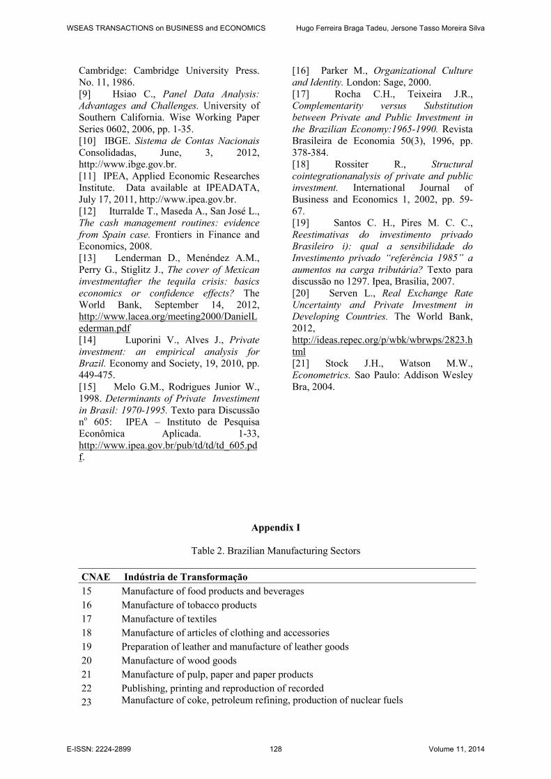
Table 2 presents twenty sectors of

the Brazilian manufacturing industry,

according to the division of activities, and

their CNAE classification, which identifies

the industrial sectors (See Appendix I).

4 Results For the econometric analysis, all variables,

except the real interest rate, were log-

linearized using the natural logarithm. The

usual estimation methods and inference

assume that these variables are stationary.

The non-stationarity of a stochastic process

is due to the existence of a unit root or

stochastic trend in autoregressive process

(AR) that generates the variable, and tests

on the unit root hypothesis, in order to help

to evaluate the presence (or absence) of

stationarity in the variables used in these

estimations.

As in the study time series, the

existence of a unit root in panel data may

cause estimated econometric relations to

become spurious. To avoid this problem,

variables were tested for the Levin unit

root, Lin and Chu (LLC), Im, Pesaran and

Smith (IPS), Fisher ADF and Fisher PP.

The test LLC assumes the existence of a

common root unit, such that ρi is the same

for all cross-sections, or all industrial

sectors (where the autocorrelation

coefficient is α = ρ - 1). The tests IPS,

Fisher-ADF and Fisher-PP, assume that the

coefficient ρi may vary according to the

industrial sector in question, characterized

by the combination of individual unit root

tests, by deriving a panel specific result.

The number of lags in each case was

determined by Schwarz’s information

criterion (SC).


E-ISSN: 2224-2899 122 Volume 11, 2014

Table 3 In Level Stationarity tests Results for Variables in the Private Investment Model

Commo Unitary Root Individual Unitary Root

LLC IPS Fisher ADF Fisher PP Integration Order

LnInv_Priv -7.99735 -5.28965 97.5515 98.5050 I(0)

LnVBPI -8.97971 -7.01750 38.7194 50.5891 I(0) ou I(1)

LnUCAP -2.51453 -1.83171 60.6368 57.6345 I(0)

R -7.29845 -3.98498 86.2369 84.3733 I(0)

LnFBKF -17.7031 -5.2271 65.7267 71.8654 I(0)

LnCred -8.4546 -3.3782 44.3610 51.1962 I(0)

LnE -1.9957 -0.0058 33.8701 36.5349 I(0)

LnEE -11.4360 -5.4583 91.0413 101.0560 I(0) ou I(1)

The analysis, presented in Table 3,

indicates that most of the series are

stationary, in other words, do not present a

unit root. For some variables, however,

such as exchange rate and industrial

production, the tests confirm the absence of

a unitary common root, but do not eliminate

the possibility of an individual unit root,

which means that the average of each panel

t-statistics indicates that the series can be

non-stationary.

In the case of the VBPI variable, a

possible explanation for this is the

heterogeneity between the industrial

sectors, which naturally have quantitative

and qualitative distinct data. It also suggests

the existence of an individual unit root.

However, as industrial production exhibits

temporal tendency, based on tests LL and

Fisher PP, we choose to use the variable in

level.

Regarding the macroeconomic

variables (R, FBKF, E, EE), the results for

the considered period (1996 -2010) indicate

that these are stationary, not showing

neither common unit root nor individual.

The only exception made is with relation to

the exchange rate series (E), which needs to

be differentiated to become stationary.

Initially, to identify the feasibility

of using the panel data methodology, the

models are estimated by Ordinary Least

Squares (OLS), with all the pooled units

(pool cross-section or pooling), in other

words, without taking into account the

possible specific sector’s effects.

The existence of specific factors in

each sector can be tested by the hypothesis

that there are significant individual effects

in the regression through a joint restrictions

F test. If the value of the F’s statistic

exceeds the critical value, there are

evidences that specific sectoral effects are

present in the estimated model [6].

The F test (Ho: fixed effects = 0)

results suggest that using the panel data

methodology provides relevant information

gain, and in this case, the OLS estimation

(pooling) may generate biased results. As

the panel data methodology is the most

appropriate, the issue now is to choose the

estimation method for fixed effects (FE) or

random effects (RE).

In this case, in which the used data

are not random extractions from a larger

sample, the fixed effects model is the most

appropriate estimation method.

Furthermore, in the fixed effects model, the

estimator is robust to the omission of

relevant explanatory variables that do not

vary over time, and even when the random

effects’ approach is valid, the estimator of

fixed effects is consistent, only less

efficiently. Therefore, the estimation by

fixed effects appears to be the most

appropriate for sector investment models.

The investment equations are

estimated by fixed effects and are robust to

the presence of multicollinearity between

variables, estimated by the Generalized

Least Squares’ method (GLS) with

weighting for individuals (industry sectors),

which makes the model also robust to the

heteroscedasticity between the individuals’

error terms. Moreover, standard deviations

were calculated by the White matrix

(period) making them robust to the serial

correlation and heteroscedasticity in the

model´s time dimension. The results are

presented in Table 4.

The results in Table 4 indicate that

the quantitative variables, Gross Value of

Industrial Production (LogVBPI) and

utilization of industrial capacity


E-ISSN: 2224-2899 123 Volume 11, 2014

(LogUCAP) were relevant in explaining

private investment. The signs found for the

estimated coefficients were positive.

The coefficient for real interest rate

(R) is positive which is contrary to the

theory of investment. However, the

magnitude of the coefficient is close to

zero, indicating that changes in the levels of

real interest rates for the period 1996 to

2010 do not affect the decision making

private sector investment.

Table 4: Investment Sectorial Equations

Estimation by Fixed Effects - Dependent Vabriable: Private Investiment 1996-2010

Explanatory

Variables (1)

EQ1 EQ2 EQ3 EQ4 EQ5 EQ6

EQ7

C -12.5731 -14.4577 -15.9587 -12.6178 -12.2551 -19.071 -17.757

[-0.3120] [-0.2579] [-0.1788] [-0.4179] [-0.8675] [-09718] [-1.172]

(0.7570) (0.7981) (0.8592) (0.6788) (0.3921) (0.3392) (0.2509)

LnVBPI(-1) 1.0619 1.1104 1.0608 1.6108 1.0622 1.1262 0.8993

[3.0732] [3.5707] [3.0361] [3.0476] [3.4756] [3.8041] [3.6193]

(0.0042) (0.0011) 0.0047 0.0046 (0.0015) (0.0007) (0.0012)

LnUCAP 1.8673 2.1943 1.8866 1.8665 1.8769 2.2629 2.2345

[0.6921] [0.1461] [0.6581] [0.7677] [1.0372] [0.5824] [0.7956]

(0.4937) (0.8847) (0.5152) (0.4482) (0.3074) (0.5647) (0.4329)

R 0.0232 0.0215 0.0258 0.0229 0.0204 0.0256 0.0322

[1.5618] [1.7484] [1.4729] [1.6920] [1.7061] [1.9003] [2.0886]

(0.1279) (0.090) (0.020) (0.1004) (0.0977) (0.0674) (0.0460)

LnCred(-1) 0.4900 0.2393 0.2763

[1.7212] [1.3930] [1.5217]

0.0949 (0.1742) (0.1393) LnFBKF (-1) 0.3376 0.4529 0.6076

[0.2179] 0.9280 [1.1694]

(0.8289) 0.3610 (0.2521)

LnE(-1) -0.0238 -0.8437 -0.3793

[-0.8581] [-0.289] [-0.733]

(0.3972) (0.7744) 0.4693

LnEE(-1) -0.3542 -0.4698 -0.5134

[-1.7488] [-1.833] [-2.026]

0.0899 (0.0770) (0.0523)

Dummy -0.2978

[-0.891]

(0.3803)

R-squared 0.9204 0.9272 0.9206 0.9222 0,9274 0.9370 0.9387

Adjusted R-

squared

0.9084 0.9135 0.9057 0.9077 0.9138 0.9174 0.9168

S.E. of

Regression

0.3382 0.3286 0.3432 0.3396 0.3281 0.3211 0.3222

Log

Likelihood

-9.8066 -8.0800 -9.7776 -9.3629 -8.0265 -5.2633 -4.7175

DW stat 1.2576 1.4946 1.2753 1.2955 1.2964 1.6326 1.5897

Prob (F-

statiscs)

0.0000 0.0000 0.0000 0.0000 0.0000 0.0000 0.0000

(1) t-statistics in brackets, followed by p-values in parentheses.


E-ISSN: 2224-2899 124 Volume 11, 2014

Despite the theoretical importance

of the investment opportunity cost, the

difficulty of finding negative and

significant coefficient for this variable is

abundantly reported in the literature [3]. In

the Brazilian case, the result found for the

interest rates effect upon private investment

can be explained by the common practice of

Brazilian companies resorting to their own

retained earnings to fund their investments.

Another possible explanation for the result

is that the interest rate may be related to the

low availability of funds.

The importance of credit

availability on the private investment is

confirmed in Equation 2 (EQ2). The results

show that increases in credit supply through

the increases of BNDES’s credit

disbursements system intended for

industrial sectors, increase the investment in

subsequent periods, unveiling the

importance of offering long-term financing

lines funded with stable amounts, and

designed to finance the private sector’s

investment projects.

The impact of public investment on

the private sector’s investment is tested in

the Equation 3 (EQ3). The variable public

investment coefficient (FBKF) is

significant and has a positive sign,

indicating that public investment tends to

complement private investment.

The estimated coefficient for the

exchange rate is negative (see EQ4 in Table

4), suggesting that a more depreciated

exchange rate discourages the import of

capital goods, at least in the short term, and

increases the financial commitments of

companies’ external indebtedness.

In relation to external debt, the

Equation 5 (EQ5) indicates the existence of

a negative relationship between investment

and external debt services. In recent years,

the existence of external constraints may

have limited private sector’s investment.

This can be explained by the increase of the

private sector’s external debt in the 1990s

and the decrease of the public sector’s

participation in the fundraising and

financing investment programs.

The Equation 6 (EQ6) tests all the

variables together, but without the dummy

variable control. The signs are coherent

with the theory and they were the same if

compared with the equations that were

tested with each variable separately.

Finally, a variable control was

included in the estimated Equation 7 for

periods of economic instability, represented

by a Dummy (D1), which assumes unit

values for the years 1997 (Asian Crisis),

1998 (Russian crisis), 1999 (Argentina

Crisis and Brazilian Exchange Rate

Devaluation) and 2008 (World Crisis) and

zero for periods without crisis. It is

observed, from the results, a negative

coefficient which indicates a negative effect

on private investment variable.

4.1 Coefficients with Fixed Effects To evaluate the specificities of each sector,

we estimated the magnitude of sectoral

fixed effects. Each estimated sector

coefficient corresponds to the pure effect of

each sector, that is, the difference in the

average investment of a particular sector,

compared to the annual average for the

sector, which is not due to the variations in

the dependent variables [6]. Thus, the

coefficient represents the actual investment

related to the specific factors of each

industry sector, regardless the included

variables in the model.

Table 5 shows the estimated

coefficients sectors. It is noted that the

coefficients signs vary according to the

sectors, and also shows the distinctive

magnitudes among the sectors and models.

The sectors that have positive coefficients

have invested relatively higher than other

sectors during the period in question,

regardless of the changes in the explanatory

variables that were considered in the model.

On the other hand, sectors that exhibit

negative coefficients are those who, without

taking into account variations in the

explanatory variables, had a level of

investment below the annual average per

sector.


E-ISSN: 2224-2899 125 Volume 11, 2014

Tabela 5 Coefficients with Fixed Effects

Sectors EQ1 EQ2 EQ3 EQ4 EQ5 EQ6 EQ7

15 0.858458 0.758991 0.852593 0.830389 0.881132 0.644522 0.597960

16 -1.477377 -1.284781 -1.426446 -1.416750 -1.504712 -1.091398 -1.089937

17 0.268283 0.255226 0.255570 0.259857 0.268896 0.233970 0.247896

18 -1.172026 -1.136179 -1.156953 -1.148507 -1.185279 -1.045358 -1.030795

19 -1.016421 -1.001485 -1.001004 -0.997517 -1.025207 -0.930483 -0.926794

20 -0.356498 -0.373803 -0.324774 -0.316142 -0.375924 -0.209512 -0.196329

21 0.815337 0.752044 0.797044 0.798238 0.820825 0.705527 0.715793

22 -0.349966 -0.210300 -0.331805 -0.328526 -0.359549 -0.157989 -0.161069

23 1.602298 1.638560 1.575055 1.567027 1.619550 1.489545 1.475811

24 0.856377 0.819212 0.846032 0.830484 0.874503 0.709110 0.676626

25 0.540872 0.548478 0.531307 0.530449 0.545114 0.507459 0.507502

26 0.280937 0.519089 0.275162 0.276563 0.281720 0.452543 0.446649

27 1.327530 1.250231 1.304057 1.296530 1.342960 1.142712 1.134296

28 -0.021863 -0.029876 -0.022579 -0.021939 -0.022197 -0.027396 -0.025343

29 0.202340 0.067000 0.156360 0.073152 0.160658 0.078905 0.214249

30 -1.581348 -1.615882 -1.574632 -1.559575 -1.597710 -1.505684 -1.470236

31 -0.171070 -0.191081 -0.173430 -0.170895 -0.172567 -0.182114 -0.174630

34 0.592623 0.532365 0.591812 0.586435 0.499989 0.380115 0.380776

35 -0.781785 -0.400374 -0.778341 -0.783552 -0.705463 -0.347895 -0.361794

36 -0.635051 -0.608970 -0.631087 -0.624206 -0.642851 -0.564619 -0.550519

R2 0.915651 0.916269 0.916617 0.917477 0.915574 0.918429 0.919195

The results presented in Table 5

indicate that sectors 15, 17, 21, 23, 24, 25,

26, 27, 29 and 34 showed positive signs. It

is observed that the intensity varies with the

inclusion of the tested variables along the

equations.

The case of sector 23 (Manufacture

of coke, petroleum refining, production of

nuclear fuels and alcohol production) which

has a coefficient value of 1.602298, in the

first equation, is symbolic in this aspect

(see Table 5). This result can be an

indication of the specifics of the petroleum

industry as for investment determinant. One

possible peculiarities inherent in sector 23

is the magnitude of the industry oil, which

requires a significance amount of

investment spending, relatively higher than

those observed in the manufacturing sectors

as a whole.

Moreover, the quest for self-

sufficiency in oil markets by Petrobras (a

government enterprise) may also have

contributed to the relatively superior

performance of investments in the sector.

Table 5 also indicate that sectors

16, 18, 19, 20, 22, 28, 30, 31, 35 and 36

showed negative signs. The negative sign

for sector 35 (Manufacture of other

transport equipment) means that it had an

investment below the annual average level

per sector. The negative sign can be

explained by several reasons: international

policies’ effects (trade liberalization and

exchange rate), international crises or also

because of its low technological intensity.

Finally, a comparative analysis

suggests that Equation 2, which tests the

hypothesis of credit constraints, presents

lower sectorial magnitude coefficients for

sector 29. The case of sector 29 (Machinery

and Equipment) is symbolic in this aspect

(see Table 5). Thus, it can infer that the

credit variable (EQ2), pointed out by the

economic theory, as an indicator to

determine investment in developing

countries, is also included in the models

that most explain investment in the

Brazilian economy.

The Brazilian industry sectors that

have reduced coefficients, close to zero,

invest relatively more according to changes

in the explanatory variables; in other words,


E-ISSN: 2224-2899 126 Volume 11, 2014

have few specific effects and are fairly well

represented by the estimated models.

5 Conclusion This study analyzed the main determinants

of private investments for a twenty

segments of the Brazilian manufacturing, as

of a panel analysis of the period comprised

between 1996 and 2010.

The estimated investment models

have confirmed the relevance of the

quantitative Gross Industrial Production

Value and Capacity Utilization variables to

explain private investment. The relationship

found between the interest rate and private

investment were positive and significant in

the sectoral models, but the coefficient

found is close to zero, suggesting that the

actual interest rate increase during the years

between 1996 and 2010, do not exert a

negative impact over the private

investment.

This empirical evidence, apparently

contradicting the economic theory, may be

related to this country’s private investment

financing conditions, which, because of the

low volume of available resources, limits

the businesses’ investments to the use of

retained earnings and bank credit.

Sectoral results also indicated that

increases in the credit supply through the

increases of BNDES credit system’s

disbursement, increased private investment

in subsequent periods, confirming the

hypothesis that Brazilian companies depend

upon long-term funds offered by official

development agencies.

The presence of instability may also

be a harmful factor for investment

financing, since instability creates

uncertainty and hinders long-term funds

sources. The negative relationship between

differentiated interest rates and investment

also reflects the entrepreneurs’ aversion to

uncertainty and instability, since the result

suggests that highly volatile foreign

exchange periods exert a negative effect

upon the private investment. A devaluated

foreign exchange rate also discourages

capital goods imports and raises the

financial liabilities of foreign-indebted

companies, which decreases investment in

the economy.

The industry-estimated coefficients

(individual sectors effects of the processing

industry) suggest that certain sectors, such

as the industry responsible for

manufacturing of other transport

equipment, showed a negative sign,

meaning that they had a level of investment

bellow the annual average per sector. On

the other hand, the other two sectors

analyzed indicate that the manufacturing

machinery and equipment sector and the

manufacturing and assembly of motor

vehicles, trailers and bodies’sectors,

showed positive signs. These sectors had

invested relatively more in accordance with

the changes in the explanatory variables.

Acknowledgments We are indebted to an anonymous reviewer

for constructive comments. The authors are

thankful to Dom Cabral Foundation and to

Prof. David Macintyre for his English

review. Remaining errors are ours.

References

[1] BACEN Economy and Finances.

Time Series, June 3, 2012,

http://www.bcb.gov.br.

[2] Bort R., Corporate cash management

handbook. New York: Warren Gorham and

Lamont RIA Group, 2004.

[3] Chirinko R.S., Business fixed

investment spending: modeling strategies,

empirical results, and policy implications.

J. of Econ. Lit. (31), 1993, pp. 1875-1911.

[4] Fernandez A., The new technologies:

afinance management tool. Actualidad

Financeira 10, 2001, pp. 35-51.

[5] Ferreira J.M.G., Investiment Evolution

in Brazil: An Econometric Analysis:

Because there was no recovery of

investment rates in the country after

stabilization of inflation in 1994? In

Dissertação de mestrado. FGV.EESP, 2005.

[6] Greene W H., Econometric Analysis.

Prentice-Hall, New Jersey. 3rd Edition,

1999.

[7] Hill R. C., Griffiths W.E., Judge G.

G., Econometrics. São Paulo: Saraiva,

1999.

[8] Hsiao C., Analysis of panel data.

Econometric Society Monographs.


E-ISSN: 2224-2899 127 Volume 11, 2014

Cambridge: Cambridge University Press.

No. 11, 1986.

[9] Hsiao C., Panel Data Analysis:

Advantages and Challenges. University of

Southern California. Wise Working Paper

Series 0602, 2006, pp. 1-35.

[10] IBGE. Sistema de Contas Nacionais

Consolidadas, June, 3, 2012,

http://www.ibge.gov.br.

[11] IPEA, Applied Economic Researches

Institute. Data available at IPEADATA,

July 17, 2011, http://www.ipea.gov.br.

[12] Iturralde T., Maseda A., San José L.,

The cash management routines: evidence

from Spain case. Frontiers in Finance and

Economics, 2008.

[13] Lenderman D., Menéndez A.M.,

Perry G., Stiglitz J., The cover of Mexican

investmentafter the tequila crisis: basics

economics or confidence effects? The

World Bank, September 14, 2012,

http://www.lacea.org/meeting2000/DanielL

ederman.pdf

[14] Luporini V., Alves J., Private

investment: an empirical analysis for

Brazil. Economy and Society, 19, 2010, pp.

449-475.

[15] Melo G.M., Rodrigues Junior W.,

1998. Determinants of Private Investiment

in Brasil: 1970-1995. Texto para Discussão

no 605: IPEA – Instituto de Pesquisa

Econômica Aplicada. 1-33,

http://www.ipea.gov.br/pub/td/td/td_605.pd

f.

[16] Parker M., Organizational Culture

and Identity. London: Sage, 2000.

[17] Rocha C.H., Teixeira J.R.,

Complementarity versus Substitution

between Private and Public Investment in

the Brazilian Economy:1965-1990. Revista

Brasileira de Economia 50(3), 1996, pp.

378-384.

[18] Rossiter R., Structural

cointegrationanalysis of private and public

investment. International Journal of

Business and Economics 1, 2002, pp. 59-

67.

[19] Santos C. H., Pires M. C. C.,

Reestimativas do investimento privado

Brasileiro i): qual a sensibilidade do

Investimento privado “referência 1985” a

aumentos na carga tributária? Texto para

discussão no 1297. Ipea, Brasilia, 2007.

[20] Serven L., Real Exchange Rate

Uncertainty and Private Investment in

Developing Countries. The World Bank,

2012,

http://ideas.repec.org/p/wbk/wbrwps/2823.h

tml

[21] Stock J.H., Watson M.W.,

Econometrics. Sao Paulo: Addison Wesley

Bra, 2004.

Appendix I

Table 2. Brazilian Manufacturing Sectors

CNAE Indústria de Transformação

15 Manufacture of food products and beverages

16 Manufacture of tobacco products

17 Manufacture of textiles

18 Manufacture of articles of clothing and accessories

19 Preparation of leather and manufacture of leather goods

20 Manufacture of wood goods

21 Manufacture of pulp, paper and paper products

22 Publishing, printing and reproduction of recorded

23 Manufacture of coke, petroleum refining, production of nuclear fuels


E-ISSN: 2224-2899 128 Volume 11, 2014

and alcohol production

24 Manufacture of chemicals

25 Manufacture of rubber and plastic

26 Manufacture of non-metallic minerals

27 Basic metallurgy

28 Manufacture of metal products - except machinery and equipment 29 Manufacture of machinery and equipment

30 Manufacture of office machinery and computer equipment

31 Manufacture of machinery, appliances and equipment 34 Manufacture and assembly of motor vehicles, trailers and bodies

35 Manufacture of other transport equipment

36 Manufacture of furniture and miscellaneous industries


E-ISSN: 2224-2899 129 Volume 11, 2014

Documents

Brazilian’s Manufacturing Sectors: Empirical Results from ... · Brazilian’s Manufacturing Sectors: Empirical Results from Panel Data ... materials and a method which ... WSEAS