Embed Size (px)
Citation preview

Branch and Bound Definitions:
• Branch and Bound is a state space search method in which all the children of a node are generated before expanding any of its children.
• Live-node: A node that has not been expanded. • It is similar to backtracking technique but uses BFS-like
search.
• Dead-node: A node that has been expanded • Solution-node
LC-Search (Least Cost Search):
• The selection rule for the next E-node in FIFO or LIFO branch-and-bound is sometimes “blind”. i.e. the selection
1
2 3 4 5
6 7 8 9
1
2 3 4 5
6 7 8 9
1
2 3 4 5
Live Node: 2, 3, 4, and 5
FIFO Branch & Bound (BFS) Children of E-node are inserted in a queue.
LIFO Branch & Bound (D-Search) Children of E-node are inserted in a stack.
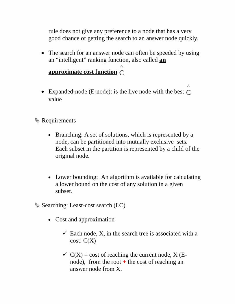
rule does not give any preference to a node that has a very good chance of getting the search to an answer node quickly.
• The search for an answer node can often be speeded by using an “intelligent” ranking function, also called an
approximate cost function C^
• Expanded-node (E-node): is the live node with the best C^
value
Requirements
• Branching: A set of solutions, which is represented by a node, can be partitioned into mutually exclusive sets. Each subset in the partition is represented by a child of the original node.
• Lower bounding: An algorithm is available for calculating a lower bound on the cost of any solution in a given subset.
Searching: Least-cost search (LC)
• Cost and approximation
Each node, X, in the search tree is associated with a cost: C(X)
C(X) = cost of reaching the current node, X (E-
node), from the root + the cost of reaching an answer node from X.

C(X) = g(X) + h(X)
Get an approximation of C(x), C^
(x) such that
C^
(x) ≤C(x), and
C^
(x) = C(x) if x is a solution-node.
The approximation part of C^
(x) is
h(x)=the cost of reaching a solution-node from X, not known.
• Least-cost search:
The next E-node is the one with least C^
Example: 8-puzzle
• Cost function: C^
= g(x) +h(x)
where h(x) = the number of misplaced tiles and g(x) = the number of moves so far
• Assumption: move one tile in any direction cost 1.

Note: In case of tie, choose the leftmost node.
1 2 3 5 6 7 8 4
1 2 3 5 8 6 7 4
Initial State Final State
532^C =+=
1 2 3 5 8 6 7 4
1 2 3 5 6 7 8 4
1 2 3 5 6 4 7 8
1 2 3 5 6 7 8 4
1 2 5 6 3 7 8 4
1 2 3 5 8 6 7 4
1 2 3 5 6 7 8 4
1 3 5 2 6 7 8 4
1 2 3 5 8 6 7 4
312^C =+=
541^C =+=
321^C =+= 541
^C =+=
532^C =+=
303^C =+=
523^C =+=
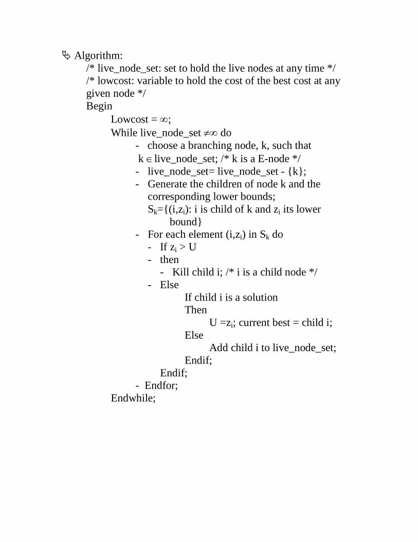
Algorithm: /* live_node_set: set to hold the live nodes at any time */ /* lowcost: variable to hold the cost of the best cost at any given node */ Begin
Lowcost = ∞; While live_node_set ≠∞ do
- choose a branching node, k, such that k ∈live_node_set; /* k is a E-node */ - live_node_set= live_node_set - {k}; - Generate the children of node k and the
corresponding lower bounds; Sk={(i,zi): i is child of k and zi its lower bound}
- For each element (i,zi) in Sk do - If zi > U - then
- Kill child i; /* i is a child node */ - Else
If child i is a solution Then U =zi; current best = child i; Else Add child i to live_node_set; Endif;
Endif; - Endfor; Endwhile;
Travelling Salesman Problem: A Branch and Bound algorithm
• Definition: Find a tour of minimum cost starting from a node S going through other nodes only once and returning to the starting point S.
• Definitions:
A row(column) is said to be reduced iff it contains at
least one zero and all remaining entries are non-negative.
A matrix is reduced iff every row and column is
reduced.
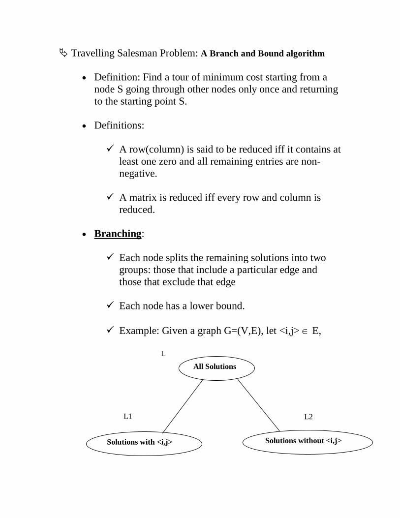
• Branching:
Each node splits the remaining solutions into two groups: those that include a particular edge and those that exclude that edge
Each node has a lower bound.
Example: Given a graph G=(V,E), let <i,j> ∈ E,
All Solutions
Solutions with <i,j> Solutions without <i,j>
L1
L
L2

• Bounding: How to compute the cost of each node?
Subtract of a constant from any row and any column does not change the optimal solution (The path).
The cost of the path changes but not the path itself.
Let A be the cost matrix of a G=(V,E).
The cost of each node in the search tree is computed as follows:
• Let R be a node in the tree and A(R) its
reduced matrix • The cost of the child (R), S:
• Set row i and column j to infinity • Set A(j,1) to infinity • Reduced S and let RCL be the
reduced cost. • C(S) = C(R) + RCL+A(i,j)
Get the reduced matrix A' of A and let L be the value subtracted from A.
L: represents the lower bound of the path solution The cost of the path is exactly reduced by L.
• What to determine the branching edge?
The rule favors a solution through left subtree rather than right subtree, i.e., the matrix is reduced by a dimension.
Note that the right subtree only sets the branching edge to infinity.
Pick the edge that causes the greatest increase in
the lower bound of the right subtree, i.e., the lower bound of the root of the right subtree is greater.
• Example: o The reduced cost matrix is done as follows:
- Change all entries of row i and column j to infinity
- Set A(j,1) to infinity (assuming the start node is 1)
- Reduce all rows first and then column of the resulting matrix

• Given the following cost matrix:
• State Space Tree:
Vertex = 3 Vertex = 5
6 7 8
10
4 5 35 53 25
Vertex = 2 Vertex = 5 Vertex = 3
3
Vertex = 2 Vertex = 5 Vertex = 4 Vertex = 3
28 50 36
52 28
25 1
2 31
9
11 28
Vertex = 3

• The TSP starts from node 1: Node 1 o Reduced Matrix: To get the lower bound of the
path starting at node 1 Row # 1: reduce by 10
Row #2: reduce 2
Row #3: reduce by 2
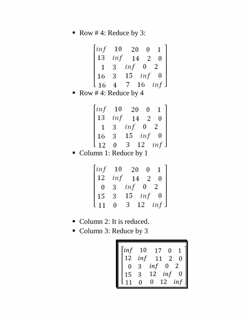
Row # 4: Reduce by 3:
Row # 4: Reduce by 4
Column 1: Reduce by 1
Column 2: It is reduced. Column 3: Reduce by 3
⎣⎢⎢⎢⎢⎡
𝑖𝑛𝑓 10 17 0 1 12 𝑖𝑛𝑓 11 2 0
0 3 𝑖𝑛𝑓 0 2 15 3 12 𝑖𝑛𝑓 0 11 0 0 12 𝑖𝑛𝑓 ⎦
⎥⎥⎥⎥⎤
⎣⎢⎢⎢⎢⎡
𝑖𝑛𝑓 10 17 0 1 12 𝑖𝑛𝑓 11 2 0
0 3 𝑖𝑛𝑓 0 2 15 3 12 𝑖𝑛𝑓 0 11 0 0 12 𝑖𝑛𝑓 ⎦
⎥⎥⎥⎥⎤
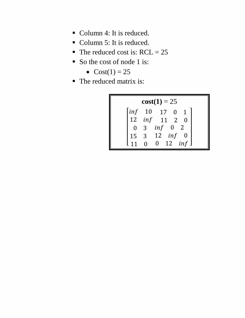
Column 4: It is reduced. Column 5: It is reduced. The reduced cost is: RCL = 25 So the cost of node 1 is:
• Cost(1) = 25 The reduced matrix is:
⎣⎢⎢⎢⎢⎡
𝑖𝑛𝑓 10 17 0 1 12 𝑖𝑛𝑓 11 2 0
0 3 𝑖𝑛𝑓 0 2 15 3 12 𝑖𝑛𝑓 0 11 0 0 12 𝑖𝑛𝑓 ⎦
⎥⎥⎥⎥⎤
cost(1) = 25
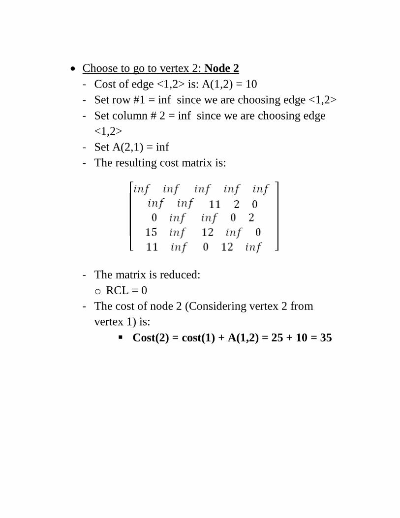
• Choose to go to vertex 2: Node 2
- Cost of edge <1,2> is: A(1,2) = 10 - Set row #1 = inf since we are choosing edge <1,2> - Set column # 2 = inf since we are choosing edge
<1,2> - Set A(2,1) = inf - The resulting cost matrix is:
- The matrix is reduced: o RCL = 0
- The cost of node 2 (Considering vertex 2 from vertex 1) is:
Cost(2) = cost(1) + A(1,2) = 25 + 10 = 35

• Choose to go to vertex 3: Node 3
- Cost of edge <1,3> is: A(1,3) = 17 (In the reduced matrix
- Set row #1 = inf since we are starting from node 1 - Set column # 3 = inf since we are choosing edge
<1,3> - Set A(3,1) = inf - The resulting cost matrix is:
• Reduce the matrix: o Rows are reduced o The columns are reduced except for column # 1:
Reduce column 1 by 11:
• The lower bound is: o RCL = 11
• The cost of going through node 3 is:

o cost(3) = cost(1) + RCL + A(1,3) = 25 + 11 + 17 = 53

• Choose to go to vertex 4: Node 4
o Remember that the cost matrix is the one that was reduced at the starting vertex 1
o Cost of edge <1,4> is: A(1,4) = 0 o Set row #1 = inf since we are starting from node
1 o Set column # 4 = inf since we are choosing edge
<1,4> o Set A(4,1) = inf o The resulting cost matrix is:
o Reduce the matrix:
Rows are reduced Columns are reduced
o The lower bound is: RCL = 0 o The cost of going through node 4 is:
cost(4) = cost(1) + RCL + A(1,4) = 25 + 0 + 0 = 25
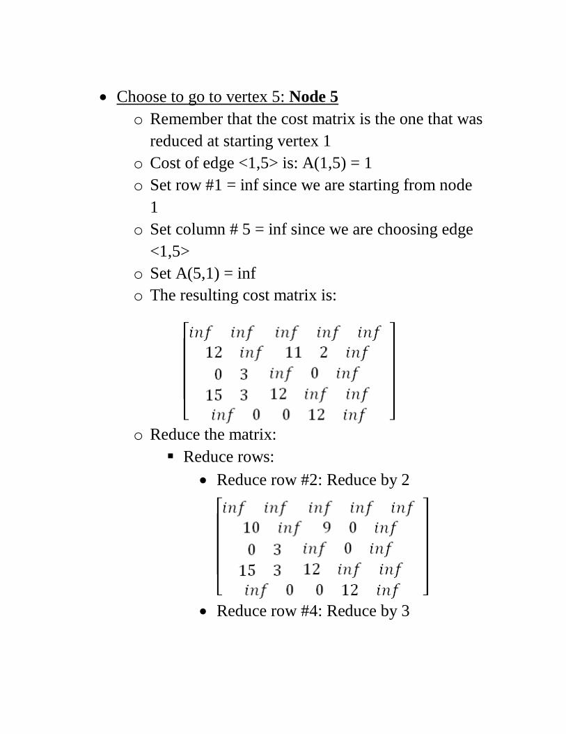
• Choose to go to vertex 5: Node 5
o Remember that the cost matrix is the one that was reduced at starting vertex 1
o Cost of edge <1,5> is: A(1,5) = 1 o Set row #1 = inf since we are starting from node
1 o Set column # 5 = inf since we are choosing edge
<1,5> o Set A(5,1) = inf o The resulting cost matrix is:
o Reduce the matrix:
Reduce rows: • Reduce row #2: Reduce by 2
• Reduce row #4: Reduce by 3

Columns are reduced
o The lower bound is:
RCL = 2 + 3 = 5 o The cost of going through node 5 is:
cost(5) = cost(1) + RCL + A(1,5) = 25 + 5 + 1 = 31
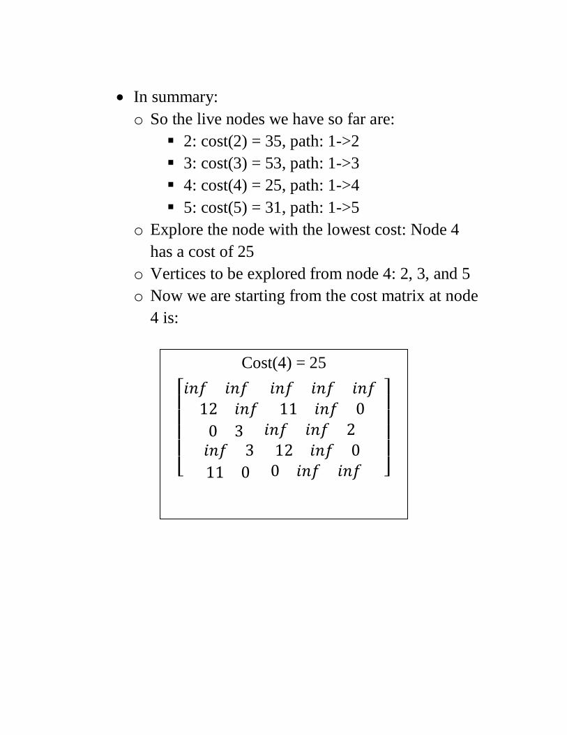
• In summary: o So the live nodes we have so far are:
2: cost(2) = 35, path: 1->2 3: cost(3) = 53, path: 1->3 4: cost(4) = 25, path: 1->4 5: cost(5) = 31, path: 1->5
o Explore the node with the lowest cost: Node 4 has a cost of 25
o Vertices to be explored from node 4: 2, 3, and 5 o Now we are starting from the cost matrix at node
4 is:
⎣⎢⎢⎢⎢⎡
𝑖𝑛𝑓 𝑖𝑛𝑓 𝑖𝑛𝑓 𝑖𝑛𝑓 𝑖𝑛𝑓
12 𝑖𝑛𝑓 11 𝑖𝑛𝑓 0 0 3 𝑖𝑛𝑓 𝑖𝑛𝑓 2 𝑖𝑛𝑓 3 12 𝑖𝑛𝑓 0 11 0 0 𝑖𝑛𝑓 𝑖𝑛𝑓 ⎦
⎥⎥⎥⎥⎤
Cost(4) = 25

• Choose to go to vertex 2: Node 6 (path is 1->4->2)
o Cost of edge <4,2> is: A(4,2) = 3 o Set row #4 = inf since we are considering edge
<4,2> o Set column # 2 = inf since we are considering
edge <4,2> o Set A(2,1) = inf o The resulting cost matrix is:
o Reduce the matrix: Rows are reduced Columns are reduced
o The lower bound is: RCL = 0 o The cost of going through node 2 is:
cost(6) = cost(4) + RCL + A(4,2) = 25 + 0 + 3 = 28

• Choose to go to vertex 3: Node 7 ( path is 1->4->3 )
o Cost of edge <4,3> is: A(4,3) = 12 o Set row #4 = inf since we are considering edge
<4,3> o Set column # 3 = inf since we are considering
edge <4,3> o Set A(3,1) = inf o The resulting cost matrix is:
o Reduce the matrix:
Reduce row #3: by 2:
Reduce column # 1: by 11
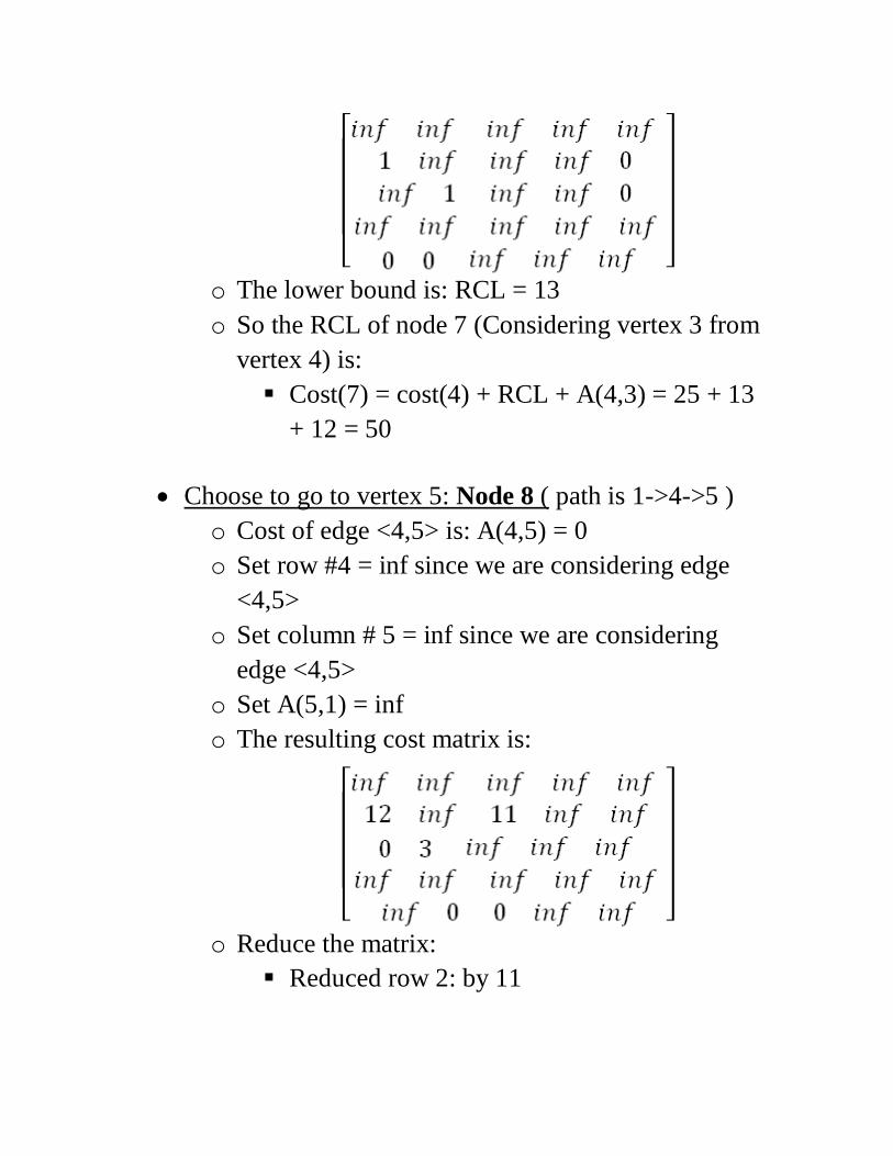
o The lower bound is: RCL = 13 o So the RCL of node 7 (Considering vertex 3 from
vertex 4) is: Cost(7) = cost(4) + RCL + A(4,3) = 25 + 13
+ 12 = 50
• Choose to go to vertex 5: Node 8 ( path is 1->4->5 ) o Cost of edge <4,5> is: A(4,5) = 0 o Set row #4 = inf since we are considering edge
<4,5> o Set column # 5 = inf since we are considering
edge <4,5> o Set A(5,1) = inf o The resulting cost matrix is:
o Reduce the matrix:
Reduced row 2: by 11

Columns are reduced o The lower bound is: RCL = 11 o So the cost of node 8 (Considering vertex 5 from
vertex 4) is: Cost(8) = cost(4) + RCL + A(4,5) = 25 + 11
+ 0 = 36

• In summary: o So the live nodes we have so far are:
2: cost(2) = 35, path: 1->2 3: cost(3) = 53, path: 1->3 5: cost(5) = 31, path: 1->5 6: cost(6) = 28, path: 1->4->2 7: cost(7) = 50, path: 1->4->3 8: cost(8) = 36, path: 1->4->5
o Explore the node with the lowest cost: Node 6
has a cost of 28 o Vertices to be explored from node 6: 3 and 5 o Now we are starting from the cost matrix at node
6 is:
⎣⎢⎢⎢⎢⎡
𝑖𝑛𝑓 𝑖𝑛𝑓 𝑖𝑛𝑓 𝑖𝑛𝑓 𝑖𝑛𝑓 𝑖𝑛𝑓 𝑖𝑛𝑓 11 𝑖𝑛𝑓 0 0 𝑖𝑛𝑓 𝑖𝑛𝑓 𝑖𝑛𝑓 2
𝑖𝑛𝑓 𝑖𝑛𝑓 𝑖𝑛𝑓 𝑖𝑛𝑓 𝑖𝑛𝑓 11 𝑖𝑛𝑓 0 𝑖𝑛𝑓 𝑖𝑛𝑓 ⎦
⎥⎥⎥⎥⎤
Cost(6) = 28
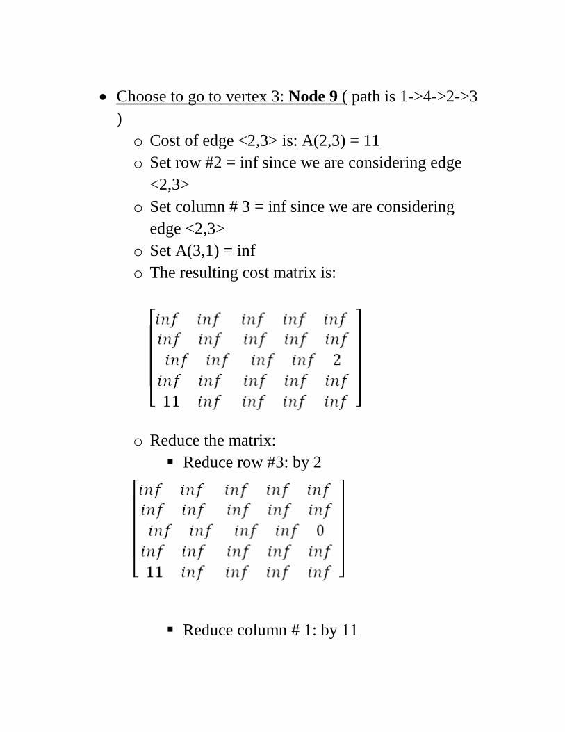
• Choose to go to vertex 3: Node 9 ( path is 1->4->2->3
) o Cost of edge <2,3> is: A(2,3) = 11 o Set row #2 = inf since we are considering edge
<2,3> o Set column # 3 = inf since we are considering
edge <2,3> o Set A(3,1) = inf o The resulting cost matrix is:
o Reduce the matrix: Reduce row #3: by 2
Reduce column # 1: by 11
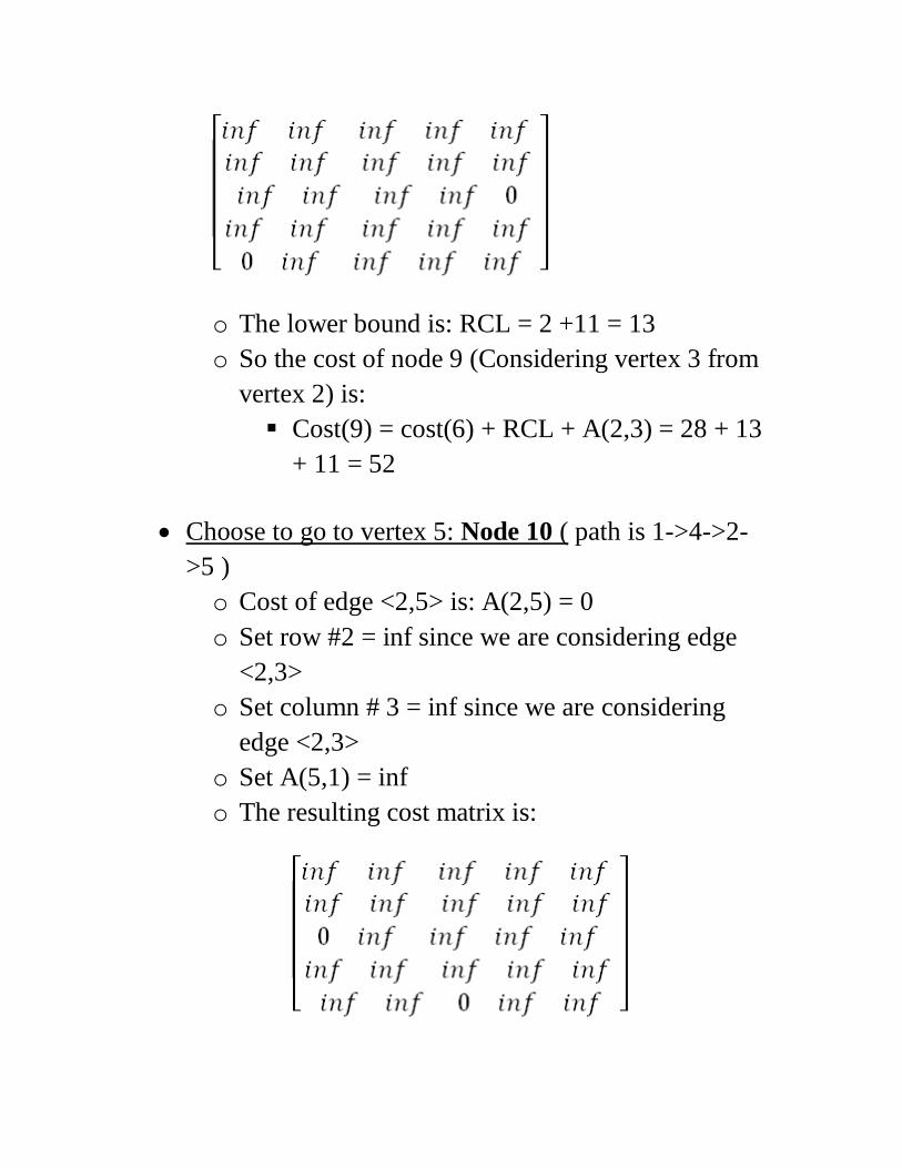
o The lower bound is: RCL = 2 +11 = 13 o So the cost of node 9 (Considering vertex 3 from
vertex 2) is: Cost(9) = cost(6) + RCL + A(2,3) = 28 + 13
+ 11 = 52
• Choose to go to vertex 5: Node 10 ( path is 1->4->2->5 ) o Cost of edge <2,5> is: A(2,5) = 0 o Set row #2 = inf since we are considering edge
<2,3> o Set column # 3 = inf since we are considering
edge <2,3> o Set A(5,1) = inf o The resulting cost matrix is:

o Reduce the matrix: Rows reduced Columns reduced
o The lower bound is: RCL = 0 o So the cost of node 10 (Considering vertex 5
from vertex 2) is: Cost(10) = cost(6) + RCL + A(2,3) = 28 + 0
+ 0 = 28
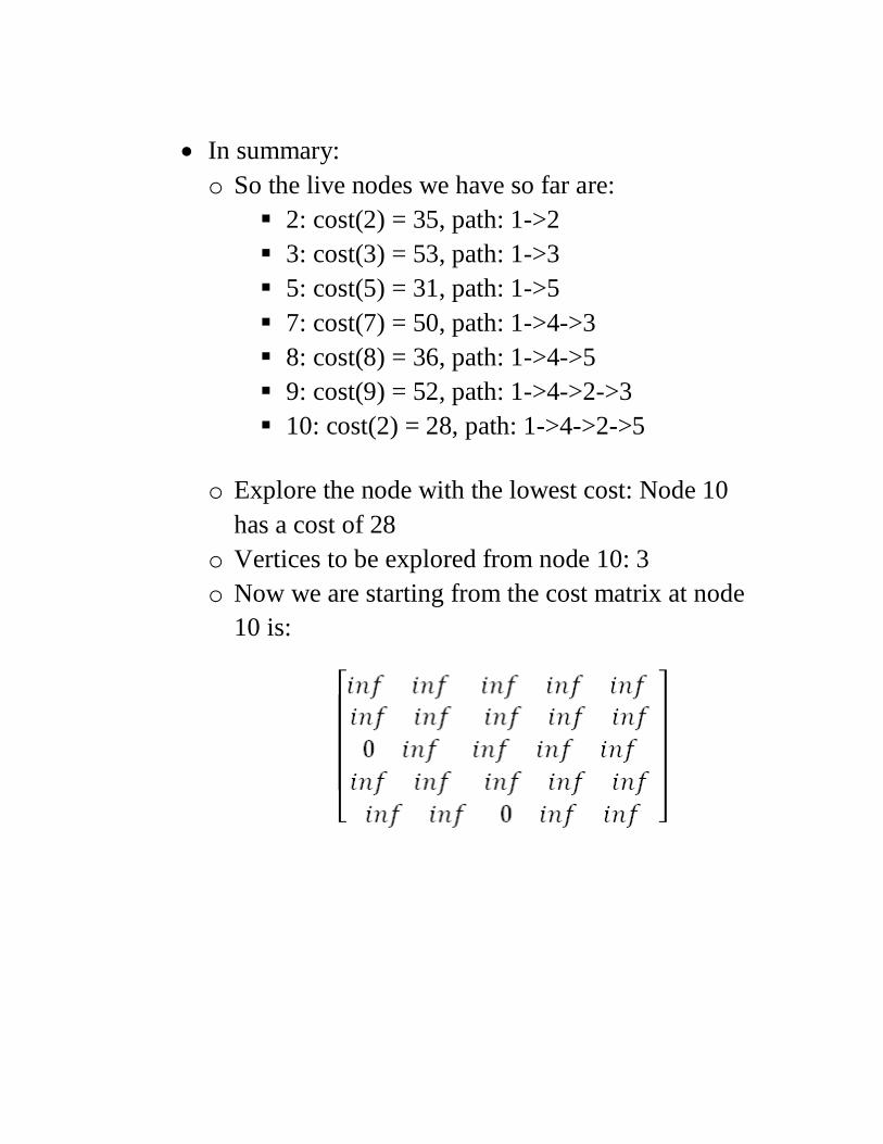
• In summary: o So the live nodes we have so far are:
2: cost(2) = 35, path: 1->2 3: cost(3) = 53, path: 1->3 5: cost(5) = 31, path: 1->5 7: cost(7) = 50, path: 1->4->3 8: cost(8) = 36, path: 1->4->5 9: cost(9) = 52, path: 1->4->2->3 10: cost(2) = 28, path: 1->4->2->5
o Explore the node with the lowest cost: Node 10
has a cost of 28 o Vertices to be explored from node 10: 3 o Now we are starting from the cost matrix at node
10 is:
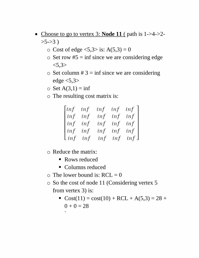
• Choose to go to vertex 3: Node 11 ( path is 1->4->2-
>5->3 ) o Cost of edge <5,3> is: A(5,3) = 0 o Set row #5 = inf since we are considering edge
<5,3> o Set column # 3 = inf since we are considering
edge <5,3> o Set A(3,1) = inf o The resulting cost matrix is:
o Reduce the matrix: Rows reduced Columns reduced
o The lower bound is: RCL = 0 o So the cost of node 11 (Considering vertex 5
from vertex 3) is: Cost(11) = cost(10) + RCL + A(5,3) = 28 +
0 + 0 = 28 `