A SURVEY ON THE ROUTING PROTOCOLS IN WIRELESS SENSOR NETWORKS

Raihan Ahmed ID-09221101

Department of Electrical and Electronic Engineering August 2010

BRAC University, Dhaka, Bangladesh

1

DECLARATION

I hereby declare that this thesis is based on the results found by myself. Materials of work found by other researcher are mentioned by reference. This thesis, neither in whole nor in part, has been previously submitted for any degree. Signature of Signature of Supervisor Author

2

ACKNOWLEDGMENTS

Special thanks to my supervisor Sadia Hamid Kazi who taught me how to think of random data clearly and logically, and for supporting this work in ways too numerous to list. Also the analysis of the data generated was only possible under her supervision. I thank her whole-heartedly for accepting the difficult task of overseeing this work to completion and for taking time out of her busy schedule to consider this work.

3

ABSTRACT Recent advances in electronics and wireless communication technologies have enabled the development of large-scale wireless sensor networks that consist of many low-power, low-cost, and small-size sensor nodes. Sensor networks hold the promise of facilitating large-scale and real-time data processing in complex environments. Some of the application areas are health, military, and home. In military, for example, the rapid deployment, self-organization, and fault tolerance characteristics of sensor networks make them a very promising technique for military command, control, communications, computing, and targeting systems. In health, sensor nodes can also be deployed to monitor patients and assist disabled patients, and etc. My area of interest for the project is the survey of different routing protocols that have been developed for secure sensor networks and find their capabilities and deficiencies and suggest the most efficient among them.

4

TABLE OF CONTENTS Page TITLE……………...........................................................................................…i DECLARATION….........................................................................................…ii ACKNOWLEDGEMENTS…………………………………………………………iii ABSTRACT………...........................................................................................iv TABLE OF CONTENTS...........................................................................…....v LIST OF TABLES............................................................................................vii LIST OF FIGURES........................................................................................viii CHAPTER I. INTRODUCTION 1.1 WIRELESS SENSOR NETWORKS…………………………………....9 1.2 COMPARISON OF MANETS AND SENSOR NETWORKS………...10 1.3 APPLICATIONS OF WIRELESS SENSOR NETWORKS……….…..10 1.4 ROUTING PROTOCOLS IN WIRELESS SENSOR NETWORKS….11 CHAPTER II. WSN ROUTING PROTOCOLS 2.1 INSENS ROUTING PROTOCOL………………………………………13 2.2 TORA……………………………………………………………………...21 2.3 LEACH……………………………………………………………….……24 . CHAPTER III. METHODOLOGY

3.1 LITERATURE REVIEW………………………………………….……...27 3.2 SIMULATION AND ANALYSIS………………………………….…….27 3.2.1 SIMULATION WITH NS-2 WITH MANNASIM…………….……….27 3.2.2 ANALYSIS USING TRACE GRAPH OUTPUT…………….………28 3.2.3 SIMULATION PARAMETERS…………………………………....…29 3.2.4 PERFORMANCE METRICS…………………………………….......29 3.2.5 SIMULATION METRICS………………………………………….….30 CHAPTER IV. ANALYSIS AND SIMULATION RESULTS 4.1 PACKET DELIVERY RATIO…………………………………………..31 4.2 ROUTING LOAD……………………………………………………..…32

5

4.3 AVERAGE END TO END DELAY………………………………….…33 CHAPTER V. CONCLUSION……………………………………………….….35 CHAPTER VI. FUTURE WORK………………………………………………..35 REFERENCES…………………………………………………………………..36

6

LIST OF TABLES Table Page

3.2.3.1 Simulation Parameters…………………………………………………29

3.2.5.1 Simulation metrics……………………………………………………...30

4.1.1 Packet Delivery Ratio for WSN Routing Protocols……………….…31

4.2.1 Routing Overhead for WSN Routing Protocols……………………...32

4.3.1 Average End to End Delay for WSN Routing Protocols……………34

7

LIST OF FIGURES Figure Page 1.1a…….………………………………………………………………………….9

1.4a………………………………………………………………………………..12

2.1a………………………………………………………………………………..14

2.1b………………………………………………………………………………..16

2.1c………………………………………………………………………………..17

2.1d………………………………………………………………………………..20

2.2a………………………………………………………………………………..22

2.3a………………………………………………………………………………..25

2.3b………………………………………………………………………………..26

4.1.2……………………………………………………………………………….31

4.2.2……………………………………………………………………………….33

4.3.2……………………………………………………………………………….34

8

1. INTRODUCTION 1.1 WIRELESS SENSOR NETWORKS A wireless sensor network (WSN) is a wireless network of many autonomous low-power, low-cost, and small-size sensor nodes that are self-organized and use sensors to co-operatively monitor complex physical or environmental conditions, such as motion, temperature, sound etc. Such sensors are generally equipped with data processing and communication capabilities and are deployed in indoor scenarios e.g.-the home and office, or outdoor scenarios like the natural, military and embedded environments. These nodes communicate with each other, sharing data collected or other vital information to monitor a specific environment. A wireless sensor network is a network of many tiny disposable low power devices, called nodes, which are spatially distributed in order to perform an application-oriented global task. These nodes form a network by communicating with each other either directly or through other nodes. One or more nodes among them will serve as sink(s) that are capable of communicating with the user either directly or through the existing wired networks. The primary component of the network is the sensor, essential for monitoring real world physical conditions such as sound, temperature, humidity, intensity, vibration, pressure, motion, pollutants etc. at different locations. The tiny sensor nodes, which consist of sensing, on board processor for data processing, and communicating components, leverage the idea of sensor networks based on collaborative effort of a large number of nodes [22].

Fig 1.1a: Wireless Sensor Network Architecture [32] The ideal wireless sensor is networked and scalable, fault tolerance, consume very little power, smart and software programmable, efficient, capable of fast

9

data acquisition, reliable and accurate over long term, cost little to purchase and required no real maintenance.[28] 1.2 COMPARISON OF MANETS AND SENSOR NETWORKS MANETS (Mobile Ad-hoc Networks) and sensor networks are two classes of the wireless Ad-hoc networks with resource constraints. MANETS typically consist of devices that have high capabilities, mobile and operate in coalitions. Sensor networks are typically deployed in specific geographical regions for tracking, monitoring and sensing. Both these wireless networks are characterized by their ad hoc nature that lack pre deployed infrastructure for computing and communication. [28] Both share some characteristics like network topology is not fixed, power is an expensive resource and nodes in the network are connected to each other by wireless communication links. WSNs differ in many fundamental ways from MANETS as mentioned below.

• Sensor networks are mainly used to collect information while MANETS are designed for distributed computing rather than information gathering.

• Sensor nodes mainly use broadcast communication paradigm whereas most MANETS are based on point-to-point communications.

• The number of nodes in sensor networks can be several orders of magnitude higher than that in MANETS.

• Sensor nodes may not have global identification (ID) because of the large amount of overhead and large number of sensors.

• Sensor nodes are much cheaper than nodes in a MANET and are usually deployed in thousands.

• Sensor nodes are limited in power, computational capacities, and memory where as nodes in a MANET can be recharged somehow.

• Usually, sensors are deployed once in their lifetime, while nodes in MANET move really in an Ad-hoc manner.

• Sensor nodes are much more limited in their computation and communication capabilities than their MANET counterparts due to their low cost.

1.3 APPLICATIONS OF WIRELESS SENSOR NETWORKS Due to their attractive characteristics, WSNs can be deployed for different purposes in trying environments. The scope of deployment which has been growing in the last decades covers many areas such as disaster management, border protection and combat field surveillance. Basically WSNs have the potential of being deployed any place where humans cannot easily access or there is danger to human life. Areas of probable usages of WSNs are

• Military

10

o Sensing intruders on basis. o Detection of enemy unit movements on land and sea. o Battle field surveillances.

• Emergency situations o Disaster management. o Fire/water detectors. o Hazardous chemical level and fires

• Physical World o Environmental monitoring of water and soil. o Habitual monitoring. o Observation of biological and artificial systems.

• Medical and Health o Sensors for blood flow, respiratory rate o ECG(electrocardiogram)

• Industrial Factory process control and industrial automation [6]. • Home Networks

o Home appliances, o Location awareness. o Person locator

1.4 ROUTING PROTOCOLS IN WIRELESS SENSOR NETWORKS: The communication between the nodes of a WSN must be governed by a set of rules (protocols) in order for them to function properly. And the data or information that they share amongst them can be tampered with by an outside intruder (adversary) for its own benefit jeopardizing the operations of the network. Thus the protocol used must provide confidentiality of the data shared among the sensor nodes in order to carry out an intended operation in the selected environment successfully. Due to the difference of wireless sensor networks from other contemporary communication and wireless ad hoc networks routing is a very challenging task in WSNs. For the deployed sheer number of sensor nodes it is impractical to build a global scheme for them. IP-based protocols cannot be applied to these networks. All applications of sensor networks have the requirement of sending the sensed data from multiple points to a common destination called sink. Resource management is required in sensor nodes regarding transmission power, storage, on-board energy and processing capacity. There are various routing protocols that have been proposed for routing data in wireless sensor networks due to such problems. The proposed mechanisms of routing consider the architecture and application requirements along with the characteristics of sensor nodes. There are few distinct routing protocols that are based on quality of service awareness or network flow whereas all other routing protocols can be classified as hierarchical or location based and data centric.

11

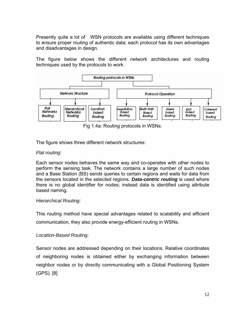
Presently quite a lot of WSN protocols are available using different techniques to ensure proper routing of authentic data; each protocol has its own advantages and disadvantages in design. The figure below shows the different network architectures and routing techniques used by the protocols to work.

Fig 1.4a: Routing protocols in WSNs.

The figure shows three different network structures: Flat routing: Each sensor nodes behaves the same way and co-operates with other nodes to perform the sensing task. The network contains a large number of such nodes and a Base Station (BS) sends queries to certain regions and waits for data from the sensors located in the selected regions. Data-centric routing is used where there is no global identifier for nodes; instead data is identified using attribute based naming.

Hierarchical Routing:

This routing method have special advantages related to scalability and efficient

communication, they also provide energy-efficient routing in WSNs.

Location-Based Routing:

Sensor nodes are addressed depending on their locations. Relative coordinates

of neighboring nodes is obtained either by exchanging information between

neighbor nodes or by directly communicating with a Global Positioning System

(GPS). [8]

12

The figure also gives an overview of the different routing techniques employed by

the protocols to work. This literature intends to survey three protocols, INSENS

(Hierarchical Routing), TORA (Flat routing), and LEACH (Hierarchical Routing),

discovering their capabilities and deficiencies and suggesting the most efficient

among them.

2. WSN ROUTING PROTOCOLS 2.1 INSENS ROUTING PROTOCOL: INSENS operates by tolerating intrusions by bypassing the malicious nodes rather than relying on traditional intrusion-detection techniques to detect them. The idea is that even if a well-equipped intruder can compromise individual sensor nodes, these intrusions can be tolerated and the network as a whole would remain functioning despite such localized intrusions so that the overall design of the WSN would remain secure. The paths are designed so that even if an intruder takes down a single node or path, independent secondary paths will exist to forward the packet to the correct destination. While a malicious node may be able to compromise a small number of nodes in its vicinity, it cannot cause widespread damage in the network. INSENS operates by having a base station possess more resources in terms of power, computation, memory, and bandwidth than the individual sensor nodes. This minimizes computation, communication, storage, and bandwidth requirements at the sensor nodes at the expense of increased computation, communication, storage, and bandwidth requirements at the base station. [1] Each message sent from a source to a destination is sent multiple times, once along each redundant path. One or more intruders along some of these paths can threaten the delivery or tamper of some of the copies of a message. However, as long as there is at least one path that is not affected by an intruder, the destination will receive at least one copy of the message that has not been tampered with so this approach works despite the presence of (undetected) intruders. INSENS's design is based on three principles: (i) Utilize redundancy to tolerate intrusions without any need for detecting the node(s) where intrusions have occurred and operate properly even in the presence of (undetected) intruders.

13

(ii)Shift the entire computational load i.e. building routing tables, or dealing with security and intrusion-tolerance issues from the individual sensor nodes to the base station thus minimizing computation, storage, and bandwidth requirements at the sensor nodes. (iii) Limit the scope of damage done by (undetected) intruders by limiting flooding and using appropriate authentication mechanisms. INSENS uses symmetric-key cryptography to implement these mechanisms. [1] To prevent DOS-style flooding attacks individual nodes are not allowed broadcasting to the entire network, only the base station is allowed to broadcast. INSENS constructs network routing for an asymmetric or hierarchical architecture consisting of a base station and sensors, unlike a peer-based routing architecture. As a result, INSENS's protocol and security architecture are far different. In INSENS, each node shares a secret key only with the base station, and not with any other nodes. The advantage is in case a node is compromised that an intruder will only have access to one secret key, rather than the secret keys of neighbors and/or other nodes throughout the network.

Fig 2.1a: Sample asymmetric WSN topology over 10 sensor nodes with multiple

paths to the base station. Moreover, setting up keys is simple in INSENS; each node needs only one secret key for authenticating itself to the base station, and one initial key for authenticating the base station to each node. Tamper detection ensures that the base station is able to glean out the correct (untampered) information from all the messages it receives from sensor nodes. INSENS employs the one-way authentication mechanism to authenticate any information sent by the base station, and appropriate integrity mechanisms to

14

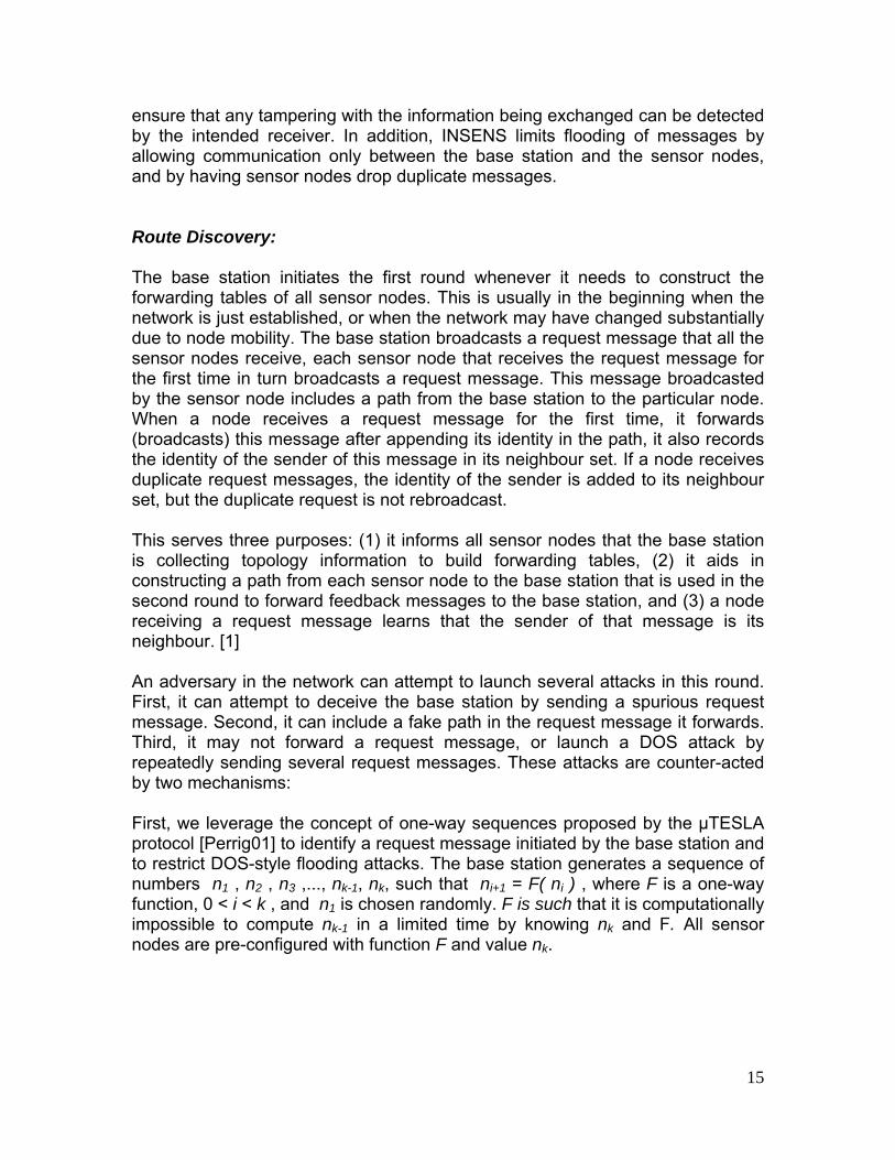
ensure that any tampering with the information being exchanged can be detected by the intended receiver. In addition, INSENS limits flooding of messages by allowing communication only between the base station and the sensor nodes, and by having sensor nodes drop duplicate messages. Route Discovery: The base station initiates the first round whenever it needs to construct the forwarding tables of all sensor nodes. This is usually in the beginning when the network is just established, or when the network may have changed substantially due to node mobility. The base station broadcasts a request message that all the sensor nodes receive, each sensor node that receives the request message for the first time in turn broadcasts a request message. This message broadcasted by the sensor node includes a path from the base station to the particular node. When a node receives a request message for the first time, it forwards (broadcasts) this message after appending its identity in the path, it also records the identity of the sender of this message in its neighbour set. If a node receives duplicate request messages, the identity of the sender is added to its neighbour set, but the duplicate request is not rebroadcast. This serves three purposes: (1) it informs all sensor nodes that the base station is collecting topology information to build forwarding tables, (2) it aids in constructing a path from each sensor node to the base station that is used in the second round to forward feedback messages to the base station, and (3) a node receiving a request message learns that the sender of that message is its neighbour. [1] An adversary in the network can attempt to launch several attacks in this round. First, it can attempt to deceive the base station by sending a spurious request message. Second, it can include a fake path in the request message it forwards. Third, it may not forward a request message, or launch a DOS attack by repeatedly sending several request messages. These attacks are counter-acted by two mechanisms: First, we leverage the concept of one-way sequences proposed by the μTESLA protocol [Perrig01] to identify a request message initiated by the base station and to restrict DOS-style flooding attacks. The base station generates a sequence of numbers n1 , n2 , n3 ,..., nk-1, nk, such that ni+1 = F( ni ) , where F is a one-way function, 0 < i < k , and n1 is chosen randomly. F is such that it is computationally impossible to compute nk-1 in a limited time by knowing nk and F. All sensor nodes are pre-configured with function F and value nk.

15

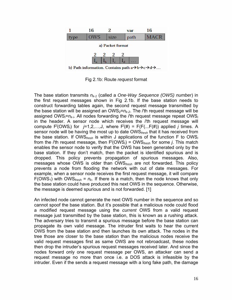
Fig 2.1b: Route request format The base station transmits nk-1 (called a One-Way Sequence (OWS) number) in the first request messages shown in Fig 2.1b. If the base station needs to construct forwarding tables again, the second request message transmitted by the base station will be assigned an OWS2=nk-2. The i'th request message will be assigned OWSi=nk-i. All nodes forwarding the i'th request message repeat OWSi in the header. A sensor node which receives the i'th request message will compute Fj(OWSi) for j=1,2,…,J, where Fj(#) = F(F(...F(#)) applied j times. A sensor node will be having the most up to date OWSfresh that it has received from the base station. If OWSfresh is within J applications of the function F to OWSi from the i'th request message, then Fj(OWSi) = OWSfresh for some j. This match enables the sensor node to verify that the OWS has been generated only by the base station. If they don’t match, then the packet is identified spurious and is dropped. This policy prevents propagation of spurious messages. Also, messages whose OWS is older than OWSfresh are not forwarded. This policy prevents a node from flooding the network with out of date messages. For example, when a sensor node receives the first request message, it will compare F(OWS1) with OWSfresh = nk. If there is a match, then the node knows that only the base station could have produced this next OWS in the sequence. Otherwise, the message is deemed spurious and is not forwarded. [1] An infected node cannot generate the next OWS number in the sequence and so cannot spoof the base station. But it’s possible that a malicious node could flood a modified request message using the current OWS from a valid request message just transmitted by the base station, this is known as a rushing attack. The adversary tries to transmit a spurious message before the base station can propagate its own valid message. The intruder first waits to hear the current OWS from the base station and then launches its own attack. The nodes in the tree those are closer to the base station than the malicious nodes receive the valid request messages first as same OWS are not rebroadcast, these nodes then drop the intruder’s spurious request messages received later. And since the nodes forward only one request message per OWS, an attacker can send a request message no more than once i.e. a DOS attack is infeasible by the intruder. Even if the sends a request message with a long fake path, the damage

16

is limited to the nodes nearest to and downstream from the intruder, the rest of the network can be considered to be not infected. In the second mechanism each node is configured with a separate secret key that is shared with the base station. A node generates a 16-byte MAC Request (MACRx) by applying a keyed MAC algorithm before sending a request message. This MAC is applied to the complete path consisting of the current node’s identity appended to the path from the incoming request message. The secret key of the node is used to generate the following MACR: MACRx =MAC ( size | path |OWS | type, Keyx ) where "|" denotes concatenation. This MACR in the request message is used to check the integrity of the path in the second round when the nodes receiving the request message need to forward a feedback message to the base station along this path (in the reverse direction). A malicious node forwarding a feedback message towards the base station with a fake path will not have the correct MAC and as a result the spurious message will be dropped. So, even if a malicious node escapes detection in the first round it will be detected in the second round. In the second round each sensor node sends a feedback message back to the base station which contains a set of identities of its neighbor nodes as well as the path to itself from the base station. Before generating a feedback message a node waits for a certain timeout interval so that a node can listen to its neighbours (upstream, peer and downstream) forwarding the same request message.

Fig 2.1c: Route feedback message from node x

17

The figure above (Fig 2.1c) shows a feedback packet, nbr_info denotes the identities of all its neighbours, path_info denotes the path to that node from the base station. For example, if node x receives the first request message for the current OWS from neighbor c, then neighbor c becomes the parent of neighbor x, namely px=c. If this first request message from c contained the path base->a->b->c, then the path returned in node x's path_info will be base->a->b->c->x. The MACF ensures that the base station will construct a correct topology, though it may be incomplete due to malicious nodes. The following keyed MACFeedbackx maintains the integrity of the packet and packets reaching the base station are guaranteed after verification to be correct and secure from tampering. The nbr_info serves to double-check against any possible tampered packets which may have somehow dodged inspection. By now, each child node will have already identified its parent as the first of its upstream neighbors to send the child a request message with the current OWS. [2] The linked chain of child-parent pairs creates a reverse unicast path from node x back to the base station (multiple paths are not available until after round three). Before forwarding a feedback message, a child node should place parent identification information into the parent_info field of the feedback message. This parent_info determines which of a child's upstream neighbours is the parent who should forward the feedback message. A child node places its parent’s MACRp into the parent_info field which it already has from the first request message it received from the parent during the first round. The MACRp has a corresponding OWS which serves as a security function as well as an addressing function. This means that spurious message cannot be forwarded as a valid address of any upstream node (required for the message to be accepted by the upstream node) isn’t available even if the attacker may have the node ID’s. An upstream node only forwards packets whose MACR matches its own MACR (selected as the child’s parent) in accordance with the OWS, otherwise the packet is dropped. An originating node only generates the MACF and intermediate nodes use the one-way function F to verify an OWS that they don’t recognize, otherwise these nodes need not recalculate a MAC and simply engage in logic comparisons of MACR's as well as memory copies of the new MACRp into the parent_info field. Only the parent_info field is modified as the message is propagated back, the path_info and nbr_info in the feedback message remain unchanged. To combat the memory exhaustion attacks the nodes store only 1 bit per node to flag whether an originating ID has been seen before; a malicious node will not be able to overflow this fixed and compact memory allocation. Hashing may reduce this memory requirement but some feedback messages may be missed that hash to the same value.

18

A second mechanism to counter-attack DOS attacks is done using rate control; thousands of phantom nodes may send feedback messages by taking advantage of the fact that in the second round nodes can in fact forward many feedback messages. Malicious nodes can send messages having a valid OWS number, any originating ID, and a valid MACRp of any upstream node. An upstream node (except the base station) has no way of distinguishing between an authentic feedback message and a spurious feedback message in this type of attacks. So even if malicious nodes send messages at a very fast rate, the upstream (correct) nodes will forward those messages only at a slower (legitimate) rate, thus preventing congestion on all the further upstream nodes. To maintain confidentiality against eavesdropping by a malicious node, the path_info (the identity field of the originating node in path_info is left unencrypted) and nbr_info is encrypted using the originating node x's secret key. Only the Type, OWS, parent_info MACRp, and identity of the originating node or sender are left unencrypted. So no topology information is revealed among the nodes but the identity of the originating node must be unencrypted so that the base station can determine to whom the topology information in the feedback packet belongs, and so that duplicate feedback packets can be spotted. In attacks where an intruder substitutes the MACR of any of its non-parental upstream nodes which divert packets away from its one valid parent INSENS’s principle allows feedback packets to simply follow another path of linked child-parent pairs that lead back to the base station. Moreover the broadcast nature of the wireless medium other upstream nodes will hear this feedback message and drop any duplicates. Therefore spurious messages cannot be forwarded by malicious child nodes towards the upstream neighbours. In the third round the base station receives all the authentic feedback messages and recomputes the MACFx and checks if there is a match. If there is a match, then the base station attempts to match the nodes listed as neighbors with prior information received by the base station. The MACR's in nbr_info received from neighbors should be consistent with the MACR's reported back to the base station; this proves that the nodes have heard each other’s individual rebroadcast which clears them of any phantom nodes. The base station now computes the forwarding tables for each node in the network. Since the base station has the complete information about the network it can perform better in selecting appropriate routes in terms of balancing the routing load on the sensor nodes and using appropriate algorithms to select redundant routes that minimize the extent of damage a malicious node may cause. The first path selection is done using Dijkstra’s shortest path algorithm and the second path is kept at the edge from the neighbours of the neighbours of the first path, if no path is found in this step the neighbours of the neighbours of the first path are included and a path is calculated from them. Again, if no path is found neighbours of the first path are also included and the path calculated from them. There could be cases where a second path is not found, so then INSENS maintains only a single path.

19

After computing the redundant paths and the forwarding tables for each node the base station forwards the forwarding tables to the respective nodes. The base station sends the tables to the nodes nearest to it and then proceeds further outwards; the redundant routing mechanism is used in this case with standard security measures.

Fig 2.1d: Routing table update message The above figure (Fig 2.1d) shows the format of the routing table message used to propagate the forwarding tables. Dest contains the address ID of the destination node x. Size contains the length of the message, and forwarding table contains the forwarding table for node x. The forwarding table entry is encrypted using the secret key of x. The MAC contains the MAC of the complete message generated using the secret key of x. A node maintains a forwarding table that has several entries, one for each route to which the node belongs. Each entry is a 3-tuple: destination, source, and immediate sender. Destination is the node id of the destination node to which a data packet is sent, source is the node id of the node that created this data packet, and immediate sender is the node id of the node that just forwarded this packet. For example, given a route from node S to D: S->a->b->c->D, the forwarding table of node a will contain an entry <D, S, S>, forwarding table of b will contain an entry <D, S, a>, and the forwarding table of c will contain an entry <D, S, b>. The node id of the immediate sender is used because a node may receive a packet with the same source and destination node many times, because each packet is forwarded over multiple routes. For example, if the other route from S to D is S->e->f->g->h->D, and b and h are neighbors, b will receive the data packet forwarded by h, which it should not forward. This is accomplished by including the immediate sender field. When the protocol INSENS is compared with a protocol having no security or intrusion tolerance, it is found that INSENS sends more packets with increasing number of nodes; this is due to the security and intrusion-tolerance issues. It is also observed that active attacks do more damage than passive attacks due to malicious nodes during route discovery. INSENS reduces the number of nodes that can be blocked over a single path routing protocol. Poor performance were obtained when the network is less dense that is nodes have fewer neighbours consequently few alternative paths. But the protocol does perform increasingly well for denser networks.

20

2.2 TORA The TORA uses a "flat", non-hierarchical routing algorithm to achieve a high degree of scalability. TORA is an on-demand routing protocol. The main objective of TORA is to limit control message propagation in the highly dynamic mobile computing environment. Control messages are localized to a very small set of nodes and it provides multiple routes for a destination. Each node has to explicitly initiate a query when it needs to send data to a particular destination. The protocol performs three basic functions: • Route creation • Route maintenance • Route erasure During the route creation and maintenance phases, nodes use a “height” metric to establish a directed acyclic graph (DAG) rooted at the destination. Thereafter, links are assigned a direction (upstream or downstream) based on the relative height metric of neighboring nodes, as shown in Fig. 5a. Routes are maintained by re-establishing routes to destination in response to topological changes. In times of node mobility the DAG route is broken, and route maintenance is necessary to re-establish a DAG rooted at the same destination.

21

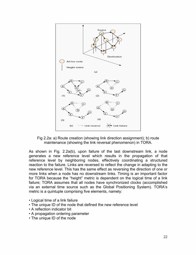
Fig 2.2a: a) Route creation (showing link direction assignment); b) route maintenance (showing the link reversal phenomenon) in TORA.

As shown in Fig. 2.2a(b), upon failure of the last downstream link, a node generates a new reference level which results in the propagation of that reference level by neighboring nodes, effectively coordinating a structured reaction to the failure. Links are reversed to reflect the change in adapting to the new reference level. This has the same effect as reversing the direction of one or more links when a node has no downstream links. Timing is an important factor for TORA because the “height” metric is dependent on the logical time of a link failure; TORA assumes that all nodes have synchronized clocks (accomplished via an external time source such as the Global Positioning System). TORA’s metric is a quintuple comprising five elements, namely: • Logical time of a link failure • The unique ID of the node that defined the new reference level • A reflection indicator bit • A propagation ordering parameter • The unique ID of the node

22

The first three elements collectively represent the reference level. A new reference level is defined each time a node loses its last downstream link due to a link failure. TORA’s route erasure phase essentially involves flooding a broadcast clear packet (CLR) throughout the network to erase invalid routes. In TORA there is a potential for oscillations to occur, especially when multiple sets of coordinating nodes are concurrently detecting partitions, erasing routes, and building new routes based on each other. Because TORA uses internodal co-ordination, its instability problem is similar to the “count-to-infinity” problem in distance-vector routing protocols, except that such oscillations. Upon the detection of a network partition, all links must be undirected to erase invalid routes and the control packets: query (QRY), update (UPD), and clear (CLR) are used to accomplish these tasks. QRY packets are used for creating routes, UPD packets are used for both creating and maintaining routes, and CLR packets are used for erasing routes. [20] A node receiving a QRY packet does one of the following:

• if its route required flag is set, this means that it doesn't have to forward the QRY, because it itself has already issued a QRY for the destination, but better discard it to prevent message overhead.

• if the node has no downstream links and the route-required flag was not set, it sets its route-required flag and rebroadcasts the QRY message.

• if a node has at least one downstream neighbour and the height for that link is null it sets its height to the minimum of the heights of the neighbour nodes, increments its d value by one and broadcasts an UPD packet.

• if the node has a downstream link and its height is non-NULL it discards the QRY packet if an UPD packet was being issued since the link became active (rr-Flag set). Otherwise it sends an UPD packet.

A node receiving an update packet updates the height value of its neighbour in the table and takes one of the following actions:

• if the reflection bit of the neighbours height is not set and its route required flag is set it sets its height for the destination to that of its neighbours but increments d by one. It then deletes the RR flag and sends an UPD message to the neighbours, so they may route through it.

• if the neighbour’s route is not valid (which is indicated by the reflection bit) or the RR flag was unset, the node only updates the entry of the neighbour’s node in its table. [24]

TORA is a “link reversal” algorithm that is best suited for networks with large dense populations of nodes. Part of the novelty of TORA stems from its creation of DAGs to aid route establishment. One of the advantages of TORA is its support for multiple routes. Route reconstruction is not necessary until all known

23

routes to a destination are deemed invalid, and hence bandwidth can potentially be conserved because of the necessity for fewer route rebuilding. However, route rebuilding in TORA may not occur as quickly as in the other algorithms due to the potential for oscillations during this period. This can lead to potentially lengthy delays while waiting for the new routes to be determined. 2.3 LEACH LEACH is based on a hierarchical clustering structure model and energy efficient cluster-based routing protocols for sensor networks. In this routing protocol, nodes self-organize themselves into several local clusters, each of which has one node serving as the cluster-head. In order to prolong the overall lifetime of the sensor networks, LEACH changes cluster heads periodically. LEACH has two main steps: the set-up phase and the steady-state phase. In the set-up phase, there are two parts, the cluster-head electing part and the cluster constructing part. After the cluster-heads have been decided on, sensor nodes (which are chosen as cluster-heads) broadcast an advertisement message that includes their node ID as the cluster-head ID to inform non-cluster sensor nodes that the chosen sensor nodes are new cluster-heads in the sensor networks. They use the carrier-sense multiple access (CSMA) medium access control (MAC) protocol to transmit this information. The non-cluster sensor nodes that receive it choose the most suitable cluster-head according to the signal strength of the advertisement message, and send a join request message to register on the chosen cluster-head. After receiving the join message, the cluster-heads make a time division multiple-access (TDMA) schedule for data exchange with non-cluster sensor nodes. Then, the cluster head informs the sensor nodes of its own cluster and the sensor nodes then start sending their data to the base station via their cluster-head during the steady-state phase. [25] However, the balance of energy consumption between all nodes in this manner does not ensure that the sensing coverage is preserved sufficiently. Nodes are deployed randomly over an entire desired area; therefore, the sensing areas of different nodes may partially overlap. When a local area has a much higher than average node density, a target location may be covered by multiple nodes. On the other hand, if the node density of a local area is much lower than the average, a target location is generally covered by only one node.

24

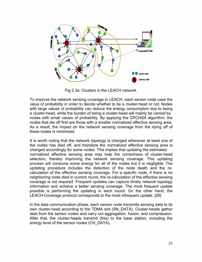
Fig 2.3a: Clusters in the LEACH network.

To improve the network sensing coverage in LEACH, each sensor node uses the value of probability in order to decide whether to be a cluster-head or not. Nodes with large values of probability can reduce the energy consumption due to being a cluster-head, while the burden of being a cluster-head will mainly be carried by nodes with small values of probability. By applying the CPCHSA algorithm, the nodes that die off first are those with a smaller normalized effective sensing area. As a result, the impact on the network sensing coverage from the dying off of these nodes is minimized. It is worth noting that the network topology is changed whenever at least one of the nodes has died off, and therefore the normalized effective sensing area is changed accordingly for some nodes. This implies that updating the estimated normalized effective sensing area may help the correctness of cluster-head selection, thereby improving the network sensing coverage. This updating process will consume some energy for all of the nodes but it is negligible. The updating procedure includes the detection of the node death and the re-calculation of the effective sensing coverage. For a specific node, if there is no neighboring node died in current round, the re-calculation of the effective sensing coverage is not required. Frequent updates can capture timely network topology information and achieve a better sensing coverage. The most frequent update possible is performing the updating in each round. On the other hand, the LEACH-Coverage protocol corresponds to the most infrequent update. [26] In the data communication phase, each sensor node transmits sensing data to its own cluster-head according to the TDMA slot (SN_DATA). Cluster-heads gather data from the sensor nodes and carry out aggregation, fusion, and compression. After that, the cluster-heads transmit (this) to the base station, including the energy level of the sensor nodes (CH_DATA).

25

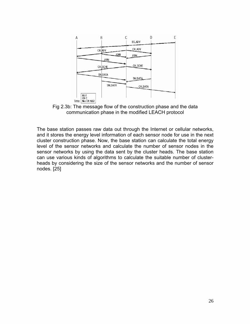
Fig 2.3b: The message flow of the construction phase and the data

communication phase in the modified LEACH protocol The base station passes raw data out through the Internet or cellular networks, and it stores the energy level information of each sensor node for use in the next cluster construction phase. Now, the base station can calculate the total energy level of the sensor networks and calculate the number of sensor nodes in the sensor networks by using the data sent by the cluster heads. The base station can use various kinds of algorithms to calculate the suitable number of cluster-heads by considering the size of the sensor networks and the number of sensor nodes. [25]

26

3. METHODOLOGY

3.1 LITERATURE REVIEW

In this step any published work or surveying of the literature of the research work done relevant about the study area is gathered for assessment, as given above.

• WSN Architecture In this step the required background information for the understanding of the subject of this thesis work is provided. Also a general understanding of the new emerging technologies from the wireless communication point of view is given in this step. It is simple to start with MANETs which are the base of WSN for the understanding of WSN. • Functionality of Routing Protocols

The explanation of the main characteristics and differences of the routing protocols and how they work for WSNs is presented in this step. This step includes how

o Selection of the path. o Control messages etc.

3.2 SIMULATION AND ANALYSIS

3.2.1 SIMULATION WITH NS-2 WITH MANNASIM

NS-2 [29] is a discrete event network simulator that has begun in 1989 as a variant of the REAL network simulator. Initially intended for wired networks, the Monarch Group at CMU have extended NS-2 to support wireless networking such as MANET and wireless LANs as well. Most MANET routing protocols are available for NS-2, as well as 802.11 MAC layer implementation. NS-2's code source is split between C++ for its core engine and OTcl, an object oriented version of TCL for configuration and simulation scripts. The combination of the two languages offers an interesting compromise between performance and ease of use. Implementation and simulation under NS-2 consists of 4 steps: (1) Implementing the protocol by adding a combination of C++ and OTcl code to NS-2's source base (2) Describing the simulation in an OTcl script (3) Running the simulation and

27

(4) Analyzing the generated trace files. NS-2 is powerful for simulating ad-hoc networks. But to simulate WSN in NS-2, it needs to have additional module to represent the protocols specific to WSN. MANNASIM [30] is a framework for WSN simulation based on NS-2. It extends NS_2 by introducing new modules for design, development and analysis of different WSN applications. The goal of MANNASIM is to develop a detailed simulation framework, which can accurately model different sensor nodes and applications while providing a versatile test bed for algorithms and protocols. MANNASIM module comprise of two solutions:

o MANNASIM Framework o Script Generator Tool

The MANNASIM Framework is a module for WSN simulation for development and analysis of different WSN applications. The Script Generator Tool (SGT) is a front end for TCL simulation scripts easy creation. SGT comes blended with MANNASIM Framework and it's written in pure Java making it platform independent. 3.2.2 ANALYSIS USING TRACE GRAPH OUTPUT There are a number of ways of collecting output or trace data on a simulation. Generally, trace data is either displayed directly during execution of the simulation, or (more commonly) stored in a file to be post-processed and analyzed. There are two primary but distinct types of monitoring capabilities currently supported by the NS-2 simulator. The first, called traces, record each individual packet as it arrives, departs, or is dropped at a link or queue. Trace objects are configured into a simulation as nodes in the network topology, usually with a TCL channel object hooked to them, representing the destination of collected data (typically a trace file in the current directory). The other types of objects, called monitors, record counts of various interesting quantities such as packet and byte arrivals, departures, etc. Monitors can monitor counts associated with all packets, or on a per-flow basis using a flow monitor [29]. Once the trace is available, it needs to be analyzed to get the statistics about the current run. NS-2 packaged with an analysis tool called xgraph. But its scope is limited to few network parameters. More over for larger traces its performance is not up to the mark. We have used the output from the trace data and used Microsoft Excel to relate the data and compute the graphs.

28

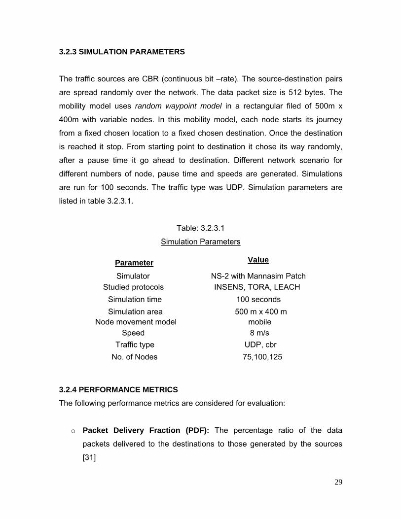
3.2.3 SIMULATION PARAMETERS

The traffic sources are CBR (continuous bit –rate). The source-destination pairs

are spread randomly over the network. The data packet size is 512 bytes. The

mobility model uses random waypoint model in a rectangular filed of 500m x

400m with variable nodes. In this mobility model, each node starts its journey

from a fixed chosen location to a fixed chosen destination. Once the destination

is reached it stop. From starting point to destination it chose its way randomly,

after a pause time it go ahead to destination. Different network scenario for

different numbers of node, pause time and speeds are generated. Simulations

are run for 100 seconds. The traffic type was UDP. Simulation parameters are

listed in table 3.2.3.1.

Table: 3.2.3.1

Simulation Parameters

Parameter Value

Simulator NS-2 with Mannasim Patch Studied protocols INSENS, TORA, LEACH

Simulation time 100 seconds Simulation area 500 m x 400 m

Node movement model mobile Speed 8 m/s

Traffic type UDP, cbr No. of Nodes 75,100,125

3.2.4 PERFORMANCE METRICS The following performance metrics are considered for evaluation:

o Packet Delivery Fraction (PDF): The percentage ratio of the data

packets delivered to the destinations to those generated by the sources

[31]

29

o Throughput: The ratio of the data packets delivered to the destinations to

those generated by the sources [31].

o Normalized routing load: The number of routing packets “transmitted”

per data packet “delivered” at the destination [31]

3.2.5 SIMULATION METRICS

Simulation metrics are listed in Table 3.2.5.1

Table: 3.2.5.1

ID Metrics Definition Formula PS Packet sent total number of packets Computed from trace file

sent by the source node

PR Packet Received Total number of packets Computed from trace file

Received by the

Destination node

PDR Packet delivery Ratio Percentage of Throughput PDR= (PR/PS)*100%

RF Routing Packets Number of routing packets Computed from trace file

sent or forwarded

NRL Normalized Number of routing packets NRL = RF/PR

Routing Load per data packets

30

4. ANALYSIS AND SIMULATION RESULTS The simulation results are shown in the following section in the form of line graphs. Graphs show comparison between the three protocols by varying different numbers of nodes on the basis of the above-mentioned metrics as a function of drop rate, received, send, time and speed.

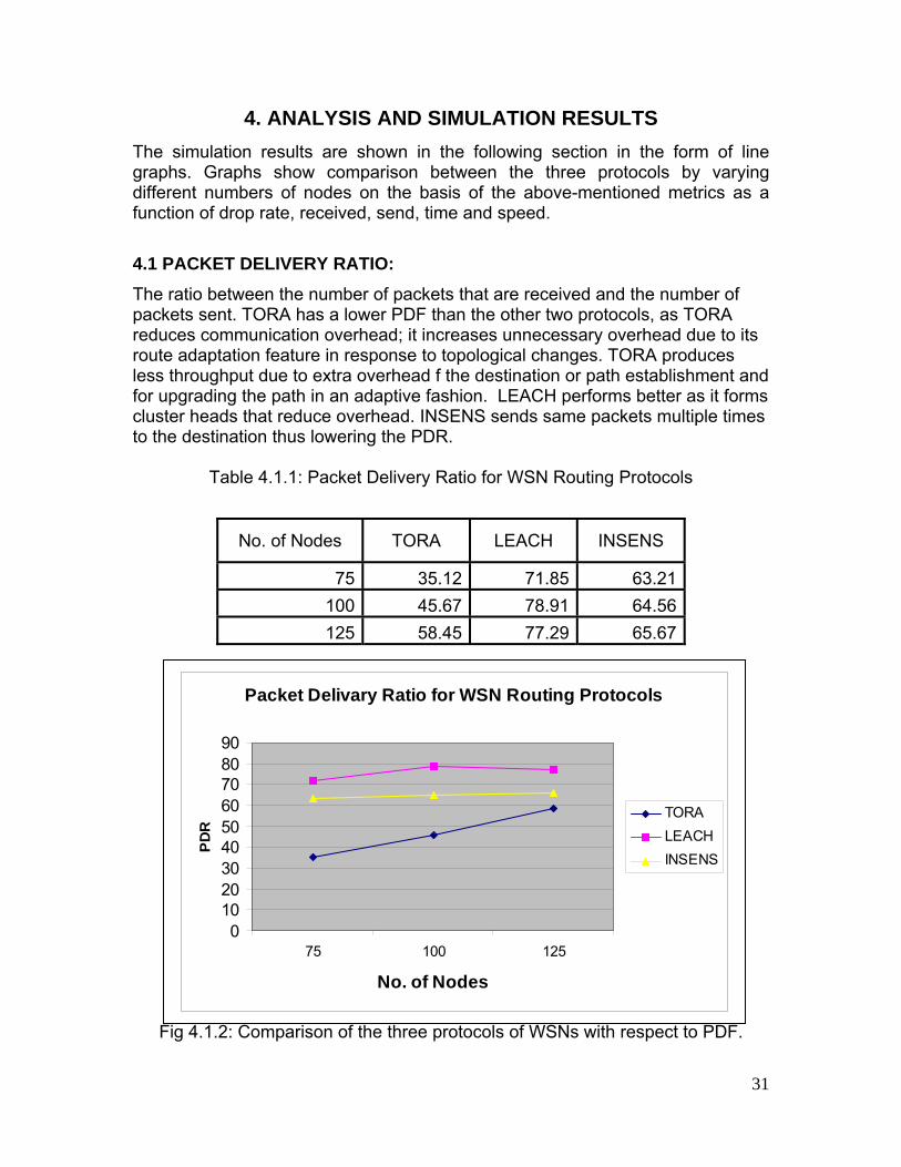
4.1 PACKET DELIVERY RATIO: The ratio between the number of packets that are received and the number of packets sent. TORA has a lower PDF than the other two protocols, as TORA reduces communication overhead; it increases unnecessary overhead due to its route adaptation feature in response to topological changes. TORA produces less throughput due to extra overhead f the destination or path establishment and for upgrading the path in an adaptive fashion. LEACH performs better as it forms cluster heads that reduce overhead. INSENS sends same packets multiple times to the destination thus lowering the PDR.

Table 4.1.1: Packet Delivery Ratio for WSN Routing Protocols

No. of Nodes TORA LEACH INSENS

75 35.12 71.85 63.21 100 45.67 78.91 64.56 125 58.45 77.29 65.67

Fig 4.1.2: Comparison of the three protocols of WSNs with respect to PDF.

Packet Delivary Ratio for WSN Routing Protocols

0102030405060708090

75 100 125

No. of Nodes

PDR

TORALEACH INSENS

31

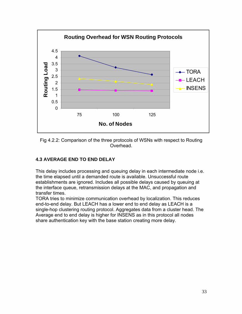
4.2 ROUTING LOAD: Routing load measures the scalability of the protocols, how much overhead a protocol can take. The routing overhead measures by the total number of control packets sent divided by the number of data packets sent successfully. As mentioned before TORA produces higher control load due to its adaptive nature. Other protocols need to re-initiate a route discovery when a link fails. TORA would be able to patch itself up around the point of failure. This feature allows TORA to scale up to larger networks but has higher overhead for smaller networks. INSENS sends more packets than the other protocols, and the difference increases with increasing numbers of nodes in the network. This difference is attributed to the overhead involved in dealing with security and intrusion-tolerance issues. LEACH performs better even with the routing load of forming clusters heads, as the area of the routing load is divided between the different clusters. There is also a co relation with the no. of nodes. LEACH and INSENS perform better with higher number of nodes.

Table 4.2.1: Routing Overhead for WSN Routing Protocols

No. of Nodes TORA LEACH INSENS

75 4.14 1.46 2.35

100 3.23 1.42 2.13

125 2.67 1.38 1.89

32

Routing Overhead for WSN Routing Protocols

00.5

11.5

22.5

33.5

44.5

75 100 125

No. of Nodes

Rou

ting

Load

TORALEACH INSENS

Fig 4.2.2: Comparison of the three protocols of WSNs with respect to Routing

Overhead.

4.3 AVERAGE END TO END DELAY This delay includes processing and queuing delay in each intermediate node i.e. the time elapsed until a demanded route is available. Unsuccessful route establishments are ignored. Includes all possible delays caused by queuing at the interface queue, retransmission delays at the MAC, and propagation and transfer times. TORA tries to minimize communication overhead by localization. This reduces end-to-end delay. But LEACH has a lower end to end delay as LEACH is a single-hop clustering routing protocol. Aggregates data from a cluster head. The Average end to end delay is higher for INSENS as in this protocol all nodes share authentication key with the base station creating more delay.

33

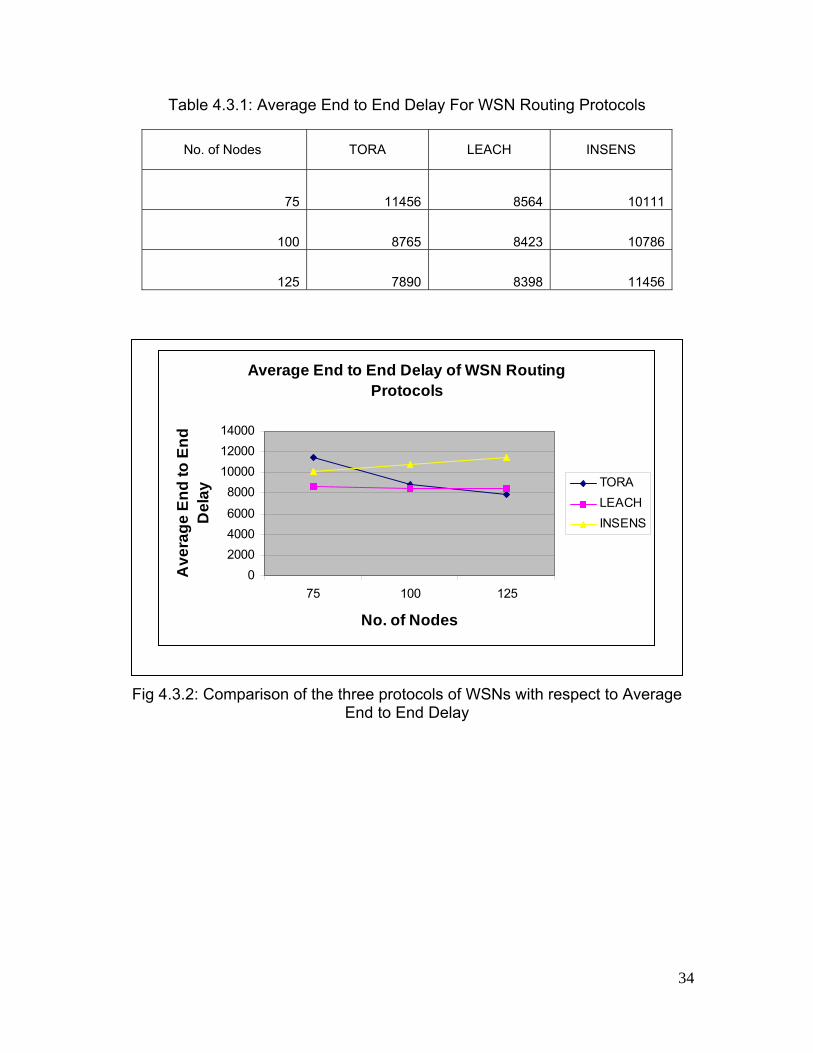
Table 4.3.1: Average End to End Delay For WSN Routing Protocols

No. of Nodes TORA LEACH INSENS

75 11456 8564 10111

100 8765 8423 10786

125 7890 8398 11456

Average End to End Delay of WSN Routing Protocols

0200040006000

8000100001200014000

75 100 125

No. of Nodes

Ave

rage

End

to E

nd

Del

ay

TORALEACH

INSENS

Fig 4.3.2: Comparison of the three protocols of WSNs with respect to Average End to End Delay

34

5. CONCLUSION:

Comparing all three routing protocols, it is seen that TORA performs less than the other two protocols. But TORA itself improves its performance when the node number increases. Other protocols need to re-initiate a route discovery when a link fails. TORA would be able to patch itself up around the point of failure. This feature allows TORA to scale up to larger networks but has higher overhead for smaller networks. LEACH has a better performance overall than the other two protocols, having a single-hop cluster based architecture. The idea of employing cluster-heads does quite help to give a higher Packet Delivery Ratio (PDR).For INSENS, as quality of service is the main issue, consequently the performance of the network was slightly degraded, although there seems to be a close competition between INSENS and LEACH, as a better QoS again means a higher PDR.

6. FUTURE WORK

A huge number of WSN protocols are available having varied network architecture and operation, each suited best for a specific environment, e.g.-WAR (Wireless Anonymous Routing), Phantom routing, SPINS etc. Comparison between these protocols can be done with additional parameters such as random node mobility, increased number of nodes etc. to determine if they can tolerate harsh and changing environments, which the protocols are prone to specially when used outdoors, and find out which one performs best in a particular environment.

35

REFERENCES

[1] Jing Deng, Richard Han, Shivakant Mishra, “INSENS: Intrusion-Tolerant Routing in Wireless Sensor Networks”, University of Colorado, Department of Computer Science Technical Report CU-CS-939-02 [2] Bryan Parno, Marl Luk, Evan Gaustad, Adrian Perrig, “Secure Sensor Network Routing: A CleanSlate Approach” [3] Gergely ´Acs, Levente Butty´an, and Istv´an Vajda, “The Security Proof of a Link-state Routing Protocol for Wireless Sensor Networks” [4] Pandurang Kamat, Yanyong Zhang, Wade Trappe, Celal Ozturk, “Enhancing Source-Location Privacy in Sensor Network Routing” [5] Magnus Bråding, “Generic, Decentralized, Unstoppable Anonymity: The Phantom Protocol” [6] Michael E. Locasto, Clayton Chen, Ajay Nambi, “WAR: Wireless Anonymous Routing” [7] Matt Blaze1, John Ioannidis2, Angelos D. Keromytis3, Tal Malkin3, and Avi Rubin, “Anonymity in Wireless Broadcast Networks” [8] http://www.wireless-sensor-networks.htm# [9] SHU JIANG, “EFFICIENT NETWORK CAMOUFLAGING IN WIRELESS NETWORKS” [10] http://finalyearprojectguide.com/projects.php?&project=nws [11] http://www.freshpatents.com/Wireless-sensor-network-and-adaptive-method-for-monitoring-the-security-thereof-dt20080410ptan20080084294.php [12] http://www.isi.edu/nsnam/ns/ns-build.html [13] Kemal Akkaya, Mohamed Younis, “A survey on routing protocols for wireless sensor networks” [14] CHEE-YEE CHONG, MEMBER, IEEE AND SRIKANTA P. KUMAR, SENIOR MEMBER, IEEE, “Sensor Networks: Evolution, Opportunities, and Challenges”

36

[15] Michael G. Reed, Paul F. Syverson, and David M. Goldschlag, “Anonymous Connections and Onion Routing” [16] X. Lin, R. Lu, H. Zhu, P. Ho, X. Shen, and Z. Cao,“ASRPAKE: An anonymous secure routing protocol with authenticated key exchange for wireless ad-hoc networks,” Proceedings of the IEEE International Conference on Communications (ICC), pp.1247-1253, June 2007. [17] http://surguy.net/bricks/elsevier/01403664/0029/0002/05002045/article.html (update ) [18] John Paul Walters, Zhengqiang Liang, Weisong Shi, and Vipin Chaudhary, “Wireless Sensor Network Security: A Survey”

[19] Xin Wu, Yufei Xu, Da Teng, “An Improved Method Based on Self-Adjusting Directed Random Walk Approach for Preserving Source-Location Privacy in Wireless Sensor Network” [20] Elizabeth M. Royer, Chai-Keong Toh, “A Review of Current Routing Protocols for Ad Hoc Mobile Wireless Networks” [21] Suhair Hafez Amer, “SOURCE-INITIATED ON-DEMAND ROUTING PROTOCOLS PERFORMANCE EVALUATION USING OPNET SIMULATION” [22] http://www.cs.ucr.edu/~krish/lec7.pdf [23] http://en.wikipedia.org/wiki/Temporally-ordered_routing_algorithm [24] http://wiki.uni.lu/secan-lab/Temporally-Ordered+Routing+Algorithm.html [25] Giljae Lee, Jonguk Kong, Minsun Lee, and Okhwan Byeon, “A Cluster Based Energy-Efficient Routing Protocol without Location Information for Sensor Networks” [26] Yuh-Ren Tsai, “Coverage-Preserving Routing Protocols for Randomly Distributed Wireless Sensor Networks”

[27] Behrouz A Frouzan, Data communication and Networking [28] Rajashree.V.Biradar ,V.C .Patil, Dr. S. R. Sawant,Dr. R. R. Mudholkar,” Classification and comparison of Routing Protocols in Wireless Sensor Networks” [29] NS-2 Documentation, http://www.isi.edu/nsnam/ns/ns-documentation.html [30] MANNASIM, frame work developed by Manna research group from Sensernet Project, MCT Brazil, 2003, http://www.mannasim.dcc.ufmg.br [31] http://www.cs.umu.se/education/examina/Rapporter/

37

[32] Wireless sensor network, http://http://en.wikipedia.org/wiki/wireless_sensor_network, January, 2008.

38