Embed Size (px)
Citation preview

5th Semester EE and EEE PID Controller in C and I
laboratory Under BPUT Odisha
Prepared BY: Dr.J.K.Moharana
Principal HIT Khurda Bhubaneswar
Odisha
PAGE NO. 1/ 5 DOC 1054REV. - 02
INSTRUCTION MANUALFOR
THERMOCOUPLE DEMONSTRATOR
MODEL NO. ME 1054
MARS' made Thermocouple Demonstrator is designed for studying the characteristics of Thermocouple for students
of instrumentation course. It allows the students to understand the concept of THERMOCOUPLE and its associate
instruments. This set-up along with this manual leads the student through various steps of theory, operation and
experimentation of the Thermocouple.
SPECIFICATIONS :
1. Transducers :
Type 'K' (Chromel - Alumel) Thermocouple.
2. Signal Conditioner Circuit :
First Stage Amplifier : DC Differential (Gain -10).
Second Stage Amplifier : Summing amplifier with zero and Gain (1-25) adjustment.
Power Source : ±5V. DC
3. Room Temperature Compensation Network :
4. Digital Panel Meter :
Display : 3 1/2 Digital LED Display.
Range : 2000, mV F.S.R.
Decimal Point : Selected at 0.01, mV.
Power : + 5, Volt D.C.
5. Milli volt Source : -10 to + 25, mVolt(Approximate)
6. Power Supply : 230Volt, + 10%, 50 Hz.
THEORY
This chapter explains the working principle of the Thermocouple and associated instrumentation is brief.
It is assumed that the student had access to some standard text book which explains the theory and working
principle in detail.
Create PDF files without this message by purchasing novaPDF printer (http://www.novapdf.com)

PAGE NO. 2/ 5 DOC 1054REV. - 02
THERMOCOUPLE :
A thermocouple is a thermoelectric device that converts thermal energy into electrical energy. The
thermocouple is used as a primary transducer for measurement of temperature, it converts temperature directly
into e.m.f. Three phenomenas which govern the behaviour of a thermocouple are the see beck effect, the Peltier
effect and the Thompson effect. While many metals and alloys exhibit the thermoelectric effect, only a small
number of them are widely applied for temperature measurement of all the metals used for thermocouples, platinum
is stable and platinum - rhodium thermocouple is the primary standard for temperature between 630.50C and
10630C. Its sensitivity is only about 6 mV/0C and is used upto 15000 C. Constantine (Ni 40%, Cu 40%) is another
alloy that is used with copper, iron or chromel or choromel (Ni 90%, Cr10%). Chopper/ Constantine thermocouple
has the maximum sensitivity of 60 mV/0C and is useful for the range from -2000C to +4000C.
In suction type thermocouple system, the thermocouple is exposed to the hot gas after it is extracted
from the hot furnace and made to flow continuously past the hot junction. The thermocouple is provided with a
radiation shield so that it does not radiate more heat to the cooler walls of the gases, than that it receivers by
radiation.
The immersion type thermocouple system is intended to measure the temperature of hot liquids and
gases by immersing it into the medium of the test fluids. For temperature upto 5000C, they are directly used if a
rapid indication is desired, otherwise a protecting tube of mild steel of sufficient length is used. The thermoelectric
characteristics of the thermocouple wires changes due to oxidation in the test fluids and the wires may be
corroded in certain fluids.
Thermocouple is the most commonly used electrical devices for temperature measurement. It is a bimetallic
devices consistants of two wires. The thermocouple provided with set - up is chromel - Alumed (K - type). If the
junction of the thermocouple is heated then the thermo - electric emf developed across its terminals depends upon
the difference in temperature between its cold and hot junction of thermocouple.
SIGNAL CONDITIONER MODULE :
The output of the thermocouple is directly fed to the input of D.C differential amplifier and then is feed to
a summing amplifier with a gain and zero adjustment to obtain output directly in engineering unit of temperature.
The final output of amplifier in fed to Digital Panel Meter.
Gain adjust Potentiometer (VR2) is given for the adjustment of amplifier gain and zero adjust potentiometer
(VR1) is given for the zero adjustment.
ROOM TEMPERATURE COMPENSATION NETWORK :
This circuit having a AD 590 (Temperature Sensor) always contain room temperature. The output of circuit
to signal conditioning circuit for measuring accurate temperature as in thermometer. It reduce the error of signal
conditioning circuit.
Create PDF files without this message by purchasing novaPDF printer (http://www.novapdf.com)
PAGE NO. 3/ 5 DOC 1054REV. - 02
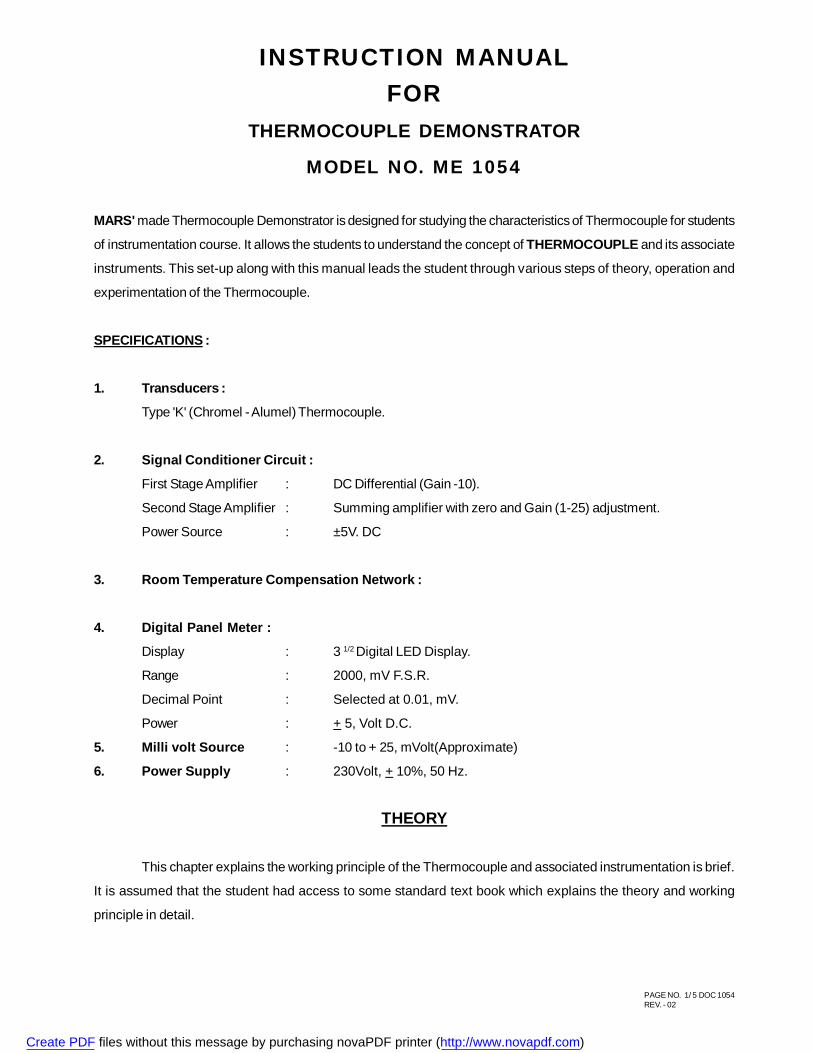
PROCEDURE
1. Connect the 220V AC Power Supply to the Demonstrator through Power Cord.
2. Keep toggle switch (provided for OC & mV ) in centre position.
3. Connect DPM positive point to TP3 & negative point to GND and set 273OK at DPM using potentiometer
VR3.
4. Remove positive point of DPM from TP3 and connect it TP2. Set VR4 to 273 + Room Temperature (0C).
E.g. 273 + 320C (32 is Room Temperature) equal to 305. Now set output at DPM using VR4 273 + 32 =
305.
5. Now put the mV - 0 - 0C switch towards 0C.
6. Now connect DPM positive point to Room Temperature compensation network output. DPM will show the
Room Temperature.
7. Set the Gain Control potentiometer VR2 to anticlockwise (i.e. set minimum gain).
8. Connect socket (To DPM) to positive of DPM.
9. Set mV - 0 - 0C switch towards mV.
10. Short the input (Thermocouple) of the set - up with a lead and measure the output on Digital Panel Meter
(DPM). It must be zero. If not, adjust it to zero with the help of VR1.
11. Connect positive & negative of mV output to positive & negative of good quality DPM. Now set mV output
to 10.0mV using set mV knob.
12. Remove the input short lead and connect the thermocouple input to mV output source.
13. Adjust 100.0on DPM using VR2. Repeat step 10 - 12 two three times for precise calibration.
14. Remove the mV (source) from the input and connect the thermocouple to the input point.
15. Take a beaker provided with instrument & fill it with water (apx. 50%). Place a immersion rod in the
beaker.
16. Keep the Thermometer & Thermocouple probe in the beaker.
Create PDF files without this message by purchasing novaPDF printer (http://www.novapdf.com)
PAGE NO. 4/ 5 DOC 1054REV. - 02
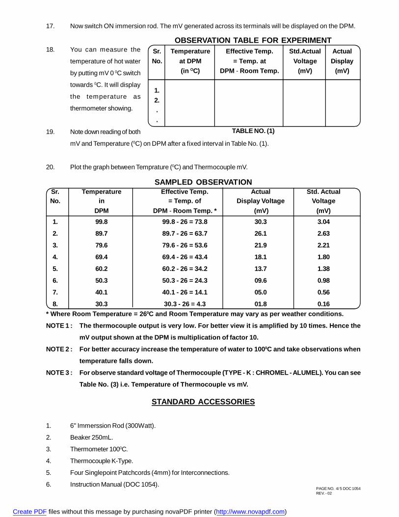
* Where Room Temperature = 260C and Room Temperature may vary as per weather conditions.
NOTE 1 : The thermocouple output is very low. For better view it is amplified by 10 times. Hence the
mV output shown at the DPM is multiplication of factor 10.
NOTE 2 : For better accuracy increase the temperature of water to 1000C and take observations when
temperature falls down.
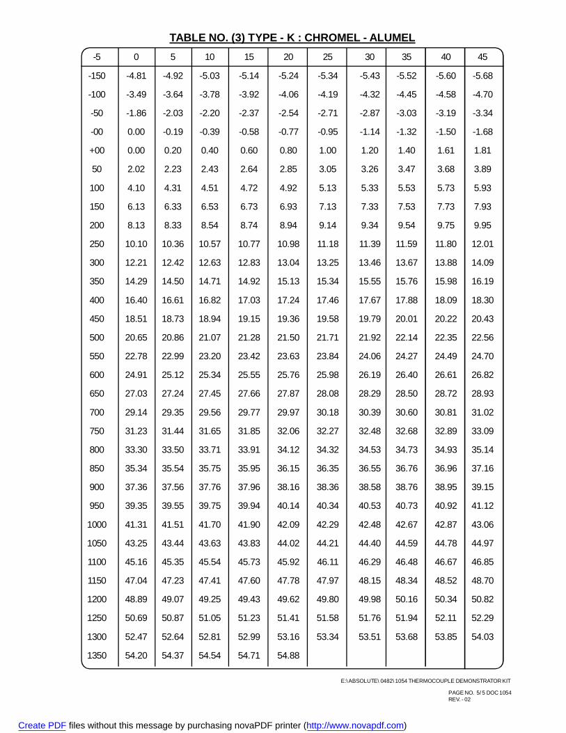
NOTE 3 : For observe standard voltage of Thermocouple (TYPE - K : CHROMEL - ALUMEL). You can see
Table No. (3) i.e. Temperature of Thermocouple vs mV.
SAMPLED OBSERVATIONSr. Temperature Effective Temp. Actual Std. ActualNo. in = Temp. of Display Voltage Voltage
DPM DPM - Room Temp. * (mV) (mV)1. 99.8 99.8 - 26 = 73.8 30.3 3.04
2. 89.7 89.7 - 26 = 63.7 26.1 2.63
3. 79.6 79.6 - 26 = 53.6 21.9 2.21
4. 69.4 69.4 - 26 = 43.4 18.1 1.80
5. 60.2 60.2 - 26 = 34.2 13.7 1.38
6. 50.3 50.3 - 26 = 24.3 09.6 0.98
7. 40.1 40.1 - 26 = 14.1 05.0 0.56
8. 30.3 30.3 - 26 = 4.3 01.8 0.16
17. Now switch ON immersion rod. The mV generated across its terminals will be displayed on the DPM.
18. You can measure the
temperature of hot water
by putting mV 0 0C switch
towards 0C. It will display
the temperature as
thermometer showing.
19. Note down reading of both
mV and Temperature (0C) on DPM after a fixed interval in Table No. (1).
20. Plot the graph between Temprature (0C) and Thermocouple mV.
STANDARD ACCESSORIES
1. 6" Immerssion Rod (300Watt).
2. Beaker 250mL.
3. Thermometer 1000C.
4. Thermocouple K-Type.
5. Four Singlepoint Patchcords (4mm) for Interconnections.
6. Instruction Manual (DOC 1054).
OBSERVATION TABLE FOR EXPERIMENTSr. Temperature Effective Temp. Std.Actual ActualNo. at DPM = Temp. at Voltage Display
(in OC) DPM - Room Temp. (mV) (mV)
1.2...
TABLE NO. (1)
Create PDF files without this message by purchasing novaPDF printer (http://www.novapdf.com)
PAGE NO. 5/ 5 DOC 1054REV. - 02
TABLE NO. (3) TYPE - K : CHROMEL - ALUMEL-5 0 5 10 15 20 25 30 35 40 45
-150 -4.81 -4.92 -5.03 -5.14 -5.24 -5.34 -5.43 -5.52 -5.60 -5.68
-100 -3.49 -3.64 -3.78 -3.92 -4.06 -4.19 -4.32 -4.45 -4.58 -4.70
-50 -1.86 -2.03 -2.20 -2.37 -2.54 -2.71 -2.87 -3.03 -3.19 -3.34
-00 0.00 -0.19 -0.39 -0.58 -0.77 -0.95 -1.14 -1.32 -1.50 -1.68
+00 0.00 0.20 0.40 0.60 0.80 1.00 1.20 1.40 1.61 1.81
50 2.02 2.23 2.43 2.64 2.85 3.05 3.26 3.47 3.68 3.89
100 4.10 4.31 4.51 4.72 4.92 5.13 5.33 5.53 5.73 5.93
150 6.13 6.33 6.53 6.73 6.93 7.13 7.33 7.53 7.73 7.93
200 8.13 8.33 8.54 8.74 8.94 9.14 9.34 9.54 9.75 9.95
250 10.10 10.36 10.57 10.77 10.98 11.18 11.39 11.59 11.80 12.01
300 12.21 12.42 12.63 12.83 13.04 13.25 13.46 13.67 13.88 14.09
350 14.29 14.50 14.71 14.92 15.13 15.34 15.55 15.76 15.98 16.19
400 16.40 16.61 16.82 17.03 17.24 17.46 17.67 17.88 18.09 18.30
450 18.51 18.73 18.94 19.15 19.36 19.58 19.79 20.01 20.22 20.43
500 20.65 20.86 21.07 21.28 21.50 21.71 21.92 22.14 22.35 22.56
550 22.78 22.99 23.20 23.42 23.63 23.84 24.06 24.27 24.49 24.70
600 24.91 25.12 25.34 25.55 25.76 25.98 26.19 26.40 26.61 26.82
650 27.03 27.24 27.45 27.66 27.87 28.08 28.29 28.50 28.72 28.93
700 29.14 29.35 29.56 29.77 29.97 30.18 30.39 30.60 30.81 31.02
750 31.23 31.44 31.65 31.85 32.06 32.27 32.48 32.68 32.89 33.09
800 33.30 33.50 33.71 33.91 34.12 34.32 34.53 34.73 34.93 35.14
850 35.34 35.54 35.75 35.95 36.15 36.35 36.55 36.76 36.96 37.16
900 37.36 37.56 37.76 37.96 38.16 38.36 38.58 38.76 38.95 39.15
950 39.35 39.55 39.75 39.94 40.14 40.34 40.53 40.73 40.92 41.12
1000 41.31 41.51 41.70 41.90 42.09 42.29 42.48 42.67 42.87 43.06
1050 43.25 43.44 43.63 43.83 44.02 44.21 44.40 44.59 44.78 44.97
1100 45.16 45.35 45.54 45.73 45.92 46.11 46.29 46.48 46.67 46.85
1150 47.04 47.23 47.41 47.60 47.78 47.97 48.15 48.34 48.52 48.70
1200 48.89 49.07 49.25 49.43 49.62 49.80 49.98 50.16 50.34 50.82
1250 50.69 50.87 51.05 51.23 51.41 51.58 51.76 51.94 52.11 52.29
1300 52.47 52.64 52.81 52.99 53.16 53.34 53.51 53.68 53.85 54.03
1350 54.20 54.37 54.54 54.71 54.88
E:\ ABSOLUTE\ 0482\ 1054 THERMOCOUPLE DEMONSTRATOR KIT
Create PDF files without this message by purchasing novaPDF printer (http://www.novapdf.com)

PAGE NO. 1/ 8 DOC 1100REV. : 02, DT. : 06.05.2010
INSTRUCTION MANUAL
FOR
PID SIMULATOR
MODEL NO. ME 1100
R
Create PDF files without this message by purchasing novaPDF printer (http://www.novapdf.com)
PAGE NO. 2/ 8 DOC 1100REV. : 02, DT. : 06.05.2010
OBJECTIVE :
“Mars” made PID Simulator Training Kit has been to study the aspects of a PID controller using
simulation.
INTRODUCTION :
This particular instrument has been designed to bring to the notice of the students all the aspects of a
simple PID controller using a simulation of a typical closed loop control system. The entire system works as
a closed loop control system, using proportional, integral and derivative mode with input in terms of a voltage.
The load on the system is simulated with the help of suitable resistances in the output circuit which try to lower
the output voltage. But in view of the closed loop performance (especially with Integral) the output is almost
restored to the desired value. The process lags are simulated is almost restored to the desired value. The
process lags are simulated with the help of R-C circuits. In the output stage, those time lags try to give
oscillating response for the system even if steady state error is zero after load change. The improvement in
dynamic response is possible with the introduction of derivative action. The proportional gain (i.e. inverse
proportional band), integral time constants and derivative time constant are made variable (both coarse and fine
controls) in an attempt to develop maximum insight into the working of a typical controller.
The unit is self contained with built in power supplies, DPM and moving coil meter. The input and
output are monitored with the help of DPM (Two ranges (0 to 2Volts & 0 to 20 volts) and moving coil meter which
gives measure of controller output, of course voltage again, and also provides insight into the dynamics of the
process. For loading, three no. of different resistances are provided. SPDT switches are provided on the panel
for operating in different modes.
General Comments and Analysis of the System.
1. Proportional Control : This control action produces an output signal (pressure in the case of pneumatic
controller voltage or current in case of electronic controller) which is proportional to the Verr and can be
expressed by
V out = Kp * Verr, Where Vout is controller Output, Kp is the gain of controller (or amplifier),
Verr = error. The transfer function of proportional controller is
Vout//Verror = kp .......................(1).
The proportional controller is characterised by presence of offset error. When load on the system
changes, there may be an offset error, because of one to one correspondence in the Verror and Voutput. For
finite gain, higher Vout can be provided with some higher error only. Hence offset error is an intrinsic feature of
the proportional action.
Create PDF files without this message by purchasing novaPDF printer (http://www.novapdf.com)

PAGE NO. 3/ 8 DOC 1100REV. : 02, DT. : 06.05.2010
2. Integral Controller : The rate of change of the output from the simple integral controller is proportional
to the error.dVout 1--------- = ki * V error = --------- *V errordt = TI
Where TI is Integral time constant in seconds. When there is a large error the controller output
changes rapidly to correct the error. As the error gets smaller, the controller output changes more slowly. This
minimizes overcorrection. As long as there is an error, the controller output will continue to change. Once the
error is zero, the output change also goes to zero. This means the controller holds the output which eliminates
the error. The transfer function of the Integral controller can be calculated as below.
dVout = ki V error dt------- ------------------ V out = ki Verror dt + V0
Where V0 is initial controller offset and hence the transfer function is
V Out/Verror = Ki / S = Ti / S ......................... (2).
The integral controller has very poor dynamic or transient response. The proportional integral controller
is an effort to combine the advantages of both i.e. good transient response from proportional and error elimination
from integral controller. The transfer function of parallel combination of P and I will be given by
Vout = kP V error +1 * Verror ........................ (3)------- ---------V error = Tis
3. Derivative Controller : The output of derivative controller can be related with rate of change of error as
per expression.
Vout = kd * dV error/dt and the transfer function is Vout/ Verr = kd x S ---------(4)
A step in error has nearly an infinite slope thus this sets the controller output into saturation. For
derivative controller, the low frequency signals, the output is very small, however, the output goes up with
frequency. The high frequency noise represents a large gain. This can be overcome by adding a series
resistance in series with Cd. The derivative controller responds to changes in error to overcome the process
inertia. It produces an output only for changes in error and hence it is mostly used in combination with other
type of controllers. Generally it is combined with PI controller to improve the dynamics of the process.
4. PID CONTROLLER
Combining the proportional, integral and derivative controller produces the three term controller. It
offers rapid proportional responses to error while having an automatic reset from an integral action to eliminate
the offset error. The derivative action stabilizes the controller and allows it to respond to rapid changes in error.
Create PDF files without this message by purchasing novaPDF printer (http://www.novapdf.com)
PAGE NO. 4/ 8 DOC 1100REV. : 02, DT. : 06.05.2010
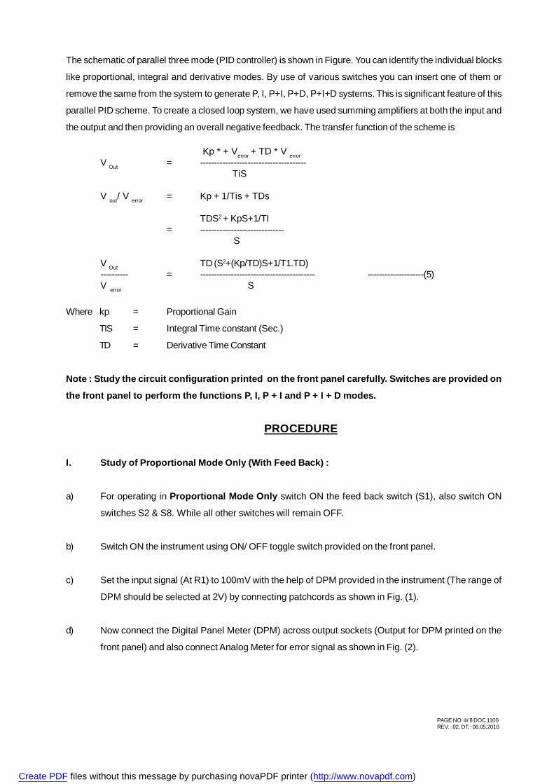
The schematic of parallel three mode (PID controller) is shown in Figure. You can identify the individual blocks
like proportional, integral and derivative modes. By use of various switches you can insert one of them or
remove the same from the system to generate P, I, P+I, P+D, P+I+D systems. This is significant feature of this
parallel PID scheme. To create a closed loop system, we have used summing amplifiers at both the input and
the output and then providing an overall negative feedback. The transfer function of the scheme is
Kp * + Verror + TD * V errorV Out = --------------------------------------
TiS
V out/ V error = Kp + 1/Tis + TDs
TDS2 + KpS+1/TI= ------------------------------
S
V Out TD (S2+(Kp/TD)S+1/T1.TD)---------- = ----------------------------------------- --------------------(5)V error S
Where kp = Proportional Gain
TIS = Integral Time constant (Sec.)
TD = Derivative Time Constant
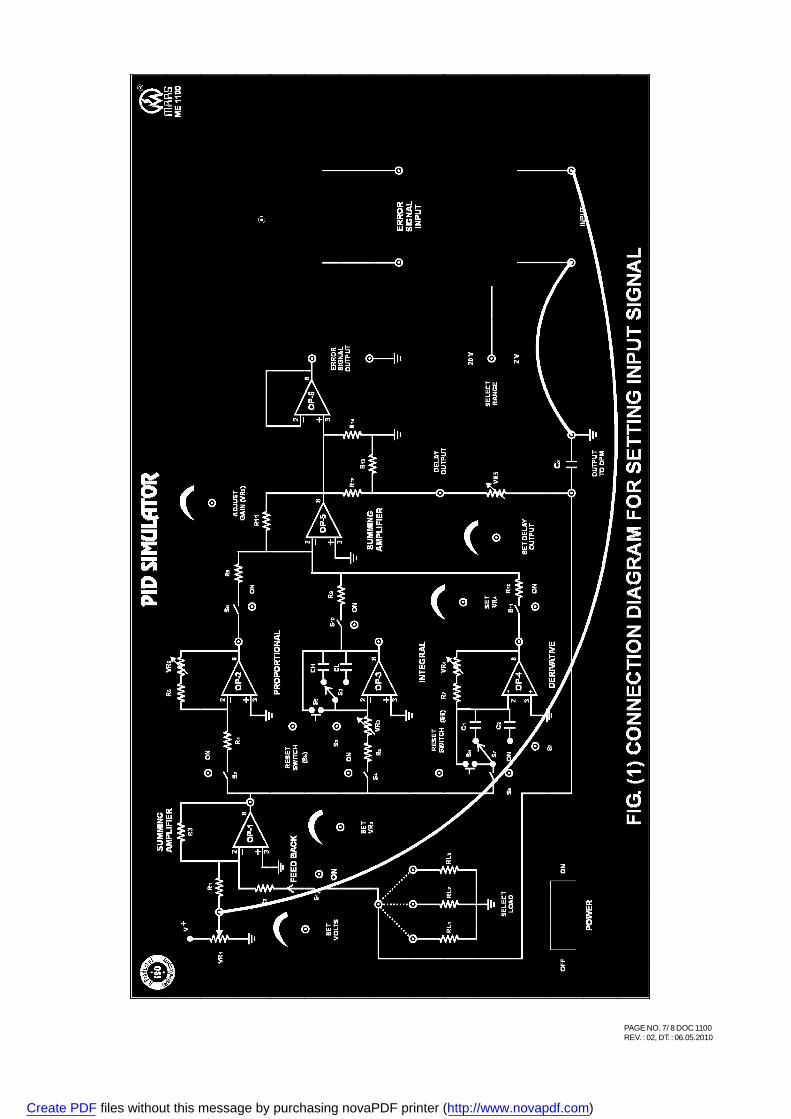
Note : Study the circuit configuration printed on the front panel carefully. Switches are provided on
the front panel to perform the functions P, I, P + I and P + I + D modes.
PROCEDURE
I. Study of Proportional Mode Only (With Feed Back) :
a) For operating in Proportional Mode Only switch ON the feed back switch (S1), also switch ON
switches S2 & S8. While all other switches will remain OFF.
b) Switch ON the instrument using ON/ OFF toggle switch provided on the front panel.
c) Set the input signal (At R1) to 100mV with the help of DPM provided in the instrument (The range of
DPM should be selected at 2V) by connecting patchcords as shown in Fig. (1).
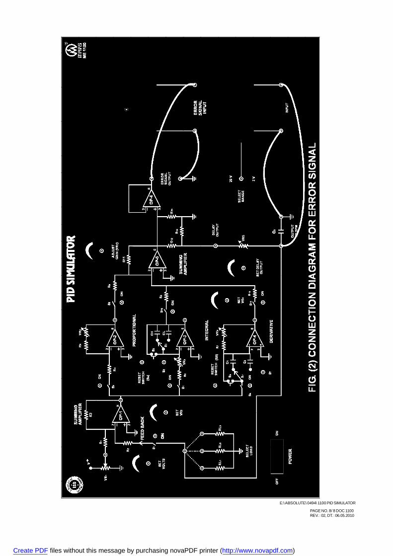
d) Now connect the Digital Panel Meter (DPM) across output sockets (Output for DPM printed on the
front panel) and also connect Analog Meter for error signal as shown in Fig. (2).
Create PDF files without this message by purchasing novaPDF printer (http://www.novapdf.com)
PAGE NO. 5/ 8 DOC 1100REV. : 02, DT. : 06.05.2010
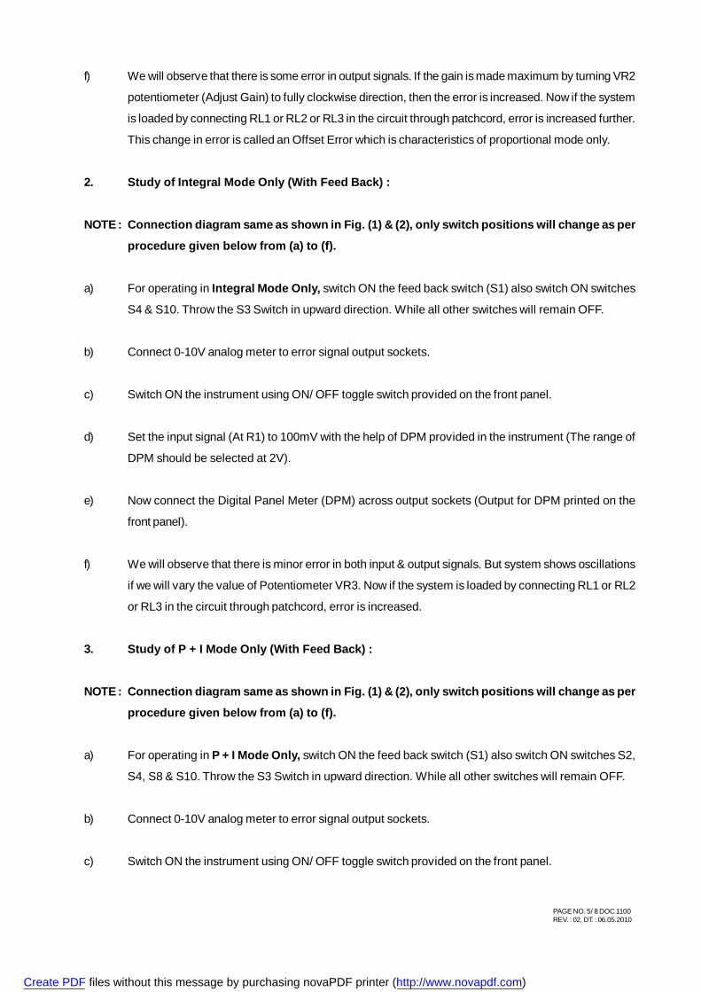
f) We will observe that there is some error in output signals. If the gain is made maximum by turning VR2
potentiometer (Adjust Gain) to fully clockwise direction, then the error is increased. Now if the system
is loaded by connecting RL1 or RL2 or RL3 in the circuit through patchcord, error is increased further.
This change in error is called an Offset Error which is characteristics of proportional mode only.
2. Study of Integral Mode Only (With Feed Back) :
NOTE : Connection diagram same as shown in Fig. (1) & (2), only switch positions will change as per
procedure given below from (a) to (f).
a) For operating in Integral Mode Only, switch ON the feed back switch (S1) also switch ON switches
S4 & S10. Throw the S3 Switch in upward direction. While all other switches will remain OFF.
b) Connect 0-10V analog meter to error signal output sockets.
c) Switch ON the instrument using ON/ OFF toggle switch provided on the front panel.
d) Set the input signal (At R1) to 100mV with the help of DPM provided in the instrument (The range of
DPM should be selected at 2V).
e) Now connect the Digital Panel Meter (DPM) across output sockets (Output for DPM printed on the
front panel).
f) We will observe that there is minor error in both input & output signals. But system shows oscillations
if we will vary the value of Potentiometer VR3. Now if the system is loaded by connecting RL1 or RL2
or RL3 in the circuit through patchcord, error is increased.
3. Study of P + I Mode Only (With Feed Back) :
NOTE : Connection diagram same as shown in Fig. (1) & (2), only switch positions will change as per
procedure given below from (a) to (f).
a) For operating in P + I Mode Only, switch ON the feed back switch (S1) also switch ON switches S2,
S4, S8 & S10. Throw the S3 Switch in upward direction. While all other switches will remain OFF.
b) Connect 0-10V analog meter to error signal output sockets.
c) Switch ON the instrument using ON/ OFF toggle switch provided on the front panel.
Create PDF files without this message by purchasing novaPDF printer (http://www.novapdf.com)
PAGE NO. 6/ 8 DOC 1100REV. : 02, DT. : 06.05.2010
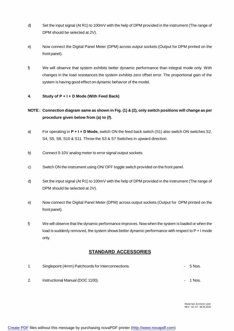
d) Set the input signal (At R1) to 100mV with the help of DPM provided in the instrument (The range of
DPM should be selected at 2V).
e) Now connect the Digital Panel Meter (DPM) across output sockets (Output for DPM printed on the
front panel).
f) We will observe that system exhibits better dynamic performance than integral mode only. With
changes in the load resistances the system exhibits zero offset error. The proportional gain of the
system is having good effect on dynamic behavior of the model.
4. Study of P + I + D Mode (With Feed Back)
NOTE : Connection diagram same as shown in Fig. (1) & (2), only switch positions will change as per
procedure given below from (a) to (f).
a) For operating in P + I + D Mode, switch ON the feed back switch (S1) also switch ON switches S2,
S4, S5, S8, S10 & S11. Throw the S3 & S7 Switches in upward direction.
b) Connect 0-10V analog meter to error signal output sockets.
c) Switch ON the instrument using ON/ OFF toggle switch provided on the front panel.
d) Set the input signal (At R1) to 100mV with the help of DPM provided in the instrument (The range of
DPM should be selected at 2V).
e) Now connect the Digital Panel Meter (DPM) across output sockets (Output for DPM printed on the
front panel).
f) We will observe that the dynamic performance improves. Now when the system is loaded or when the
load is suddenly removed, the system shows better dynamic performance with respect to P + I mode
only.
STANDARD ACCESSORIES
1. Singlepoint (4mm) Patchcords for Interconnections. - 5 Nos.
2. Instructional Manual (DOC 1100). - 1 Nos.
Create PDF files without this message by purchasing novaPDF printer (http://www.novapdf.com)
PAGE NO. 7/ 8 DOC 1100REV. : 02, DT. : 06.05.2010
Create PDF files without this message by purchasing novaPDF printer (http://www.novapdf.com)
PAGE NO. 8/ 8 DOC 1100REV. : 02, DT. : 06.05.2010
E:\ ABSOLUTE\ 0494\ 1100 PID SIMULATOR
Create PDF files without this message by purchasing novaPDF printer (http://www.novapdf.com)
PAGE NO. 1/ 6 DOC 2202REV. : 02, DT. 15.06.2010
INSTRUCTION MANUALFOR
KELVIN DOUBLE BRIDGE (INDUSTRIAL)
MODEL NO. ME 2202
'MARS' made Kelvin Double Bridge has been designed to calculate the value of low resistances.
The instruments comprises of the following builtin parts :
1. Multiplier dial is provided on the front panel with differents ranges (X0.01, X0.1, X1, X10 & X100).
2. Standard resistance dial & slide wire dial are also provided on the front panel.
3. Two press keys are provided on the front panel marked as course & Fine.
4. Current reversing switch is provided on the front panel to get the diflection on left or right hand side in
a Galvanometer with centred OFF position.
5. Terminals are provided on the front panel to connect Galvanometer & DC Source.
6. Another four terminals are provided on the left side of panel out of these +C +P & -C
-P are connected
and between +P -P unknown resistance is to be connected.
Introduction of the Front Panel control and other Function :
1. Galvanometer :
Two terminals are provided on the panel to connect Galvanometer with instrument.
2. DC Source Terminals :
Two terminals are provided on the panel to connect the high ampere DC Source of (10Volts /
10Amps.) or Battery with instrument. Positive is connected to Red terminal & Negative is connected
to Black terminal.
3. Multiplier Dial :
Five different ranges (X0.01, X0.1, X1, X10 & X100) are provided. With the help of these ranges
you will get low resistance from 0.2m to 11.
Create PDF files without this message by purchasing novaPDF printer (http://www.novapdf.com)
PAGE NO. 2/ 6 DOC 2202REV. : 02, DT. 15.06.2010
4. Standard Resistance Dial :
Ten standard resistance coils are connected with this dial. Each coil having a fixed resistance
of 0.01.
5. Press Key (Intial & Final) :
Two press keys are provided on the panel marked Intial & Final. Two press key are provided to
protect the Galvanometer from high current. First you adjust the approximate value of resistance and
then press the Intial & Final key to set the Galvanometer at null point.
6. Lock Knob :
A knob is provided on the slide wire dial is lock it with graduate scale.
7. Mounting Knob :
This knob is bigger than the earlier knob, is also fitted on the slide wire dial. This is privided to
compensate for any lead resistance and to obtain correct zero/ null point before start of measurements.
8. Slide Wire Dial :
The first coil of (0.01) of the standard resistance is further divided equally in 500 parts. The
one division of this dial is equal to 0.00002. One more small knob is fitted on this dial. This is
provided to compensate for any lead resistance and to obtain correct zero/ null point before start of
measurement.
9. Current Reversing Switch :
This switch is provided to get the spot on the Galvanometer on left or right hand side of the
scale. If the switch is put at 'Forward' position, the spot apears on left hand side of the scale and if the
switch is put at 'Revrse' position, the spot apears on the right hand side of the scale. The position
between 'Forward' & 'Reverse' of the switch is OFF position.
10. Conductivity Attachment :
For thick wires whose unknown resistance to known, a special type of accesory "Conductivity
Attachment" is used. By using this we can find out the resistance of wire whose length is 50cm.
THEORY
Kelvin is one of the best method for the precise measurement of low resistance. It is a development of
the Wheatstone Bridge method by which the errorsdue to contacts and lead resistances are eliminated. This
bridge is quite simple and easy to operate. This instrument can measure low resistance an order of 0.2m to
11with an accuracy of 0.5%. Fix the resistance (Whose value is to be measured) in the test terminals and
with the help of decade dials, slide wire and ratio selector, obtain the null point. the reading of decade dial, slide
Create PDF files without this message by purchasing novaPDF printer (http://www.novapdf.com)
PAGE NO. 3/ 6 DOC 2202REV. : 02, DT. 15.06.2010
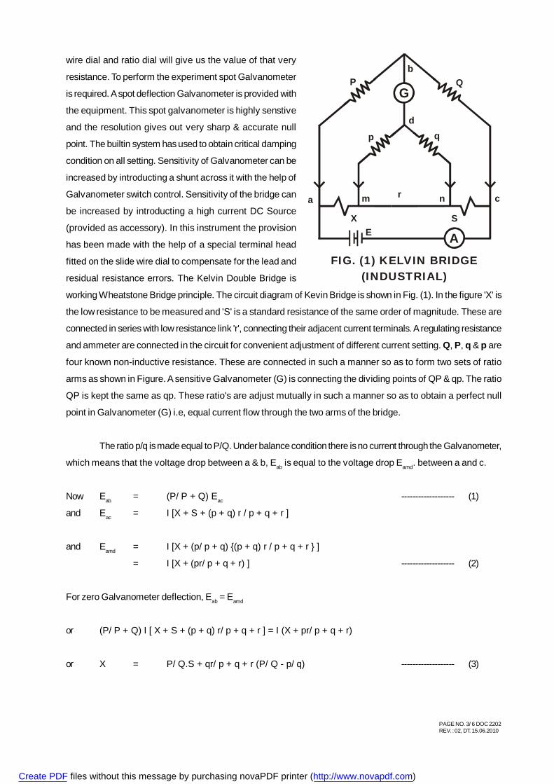
wire dial and ratio dial will give us the value of that very
resistance. To perform the experiment spot Galvanometer
is required. A spot deflection Galvanometer is provided with
the equipment. This spot galvanometer is highly senstive
and the resolution gives out very sharp & accurate null
point. The builtin system has used to obtain critical damping
condition on all setting. Sensitivity of Galvanometer can be
increased by introducting a shunt across it with the help of
Galvanometer switch control. Sensitivity of the bridge can
be increased by introducting a high current DC Source
(provided as accessory). In this instrument the provision
has been made with the help of a special terminal head
fitted on the slide wire dial to compensate for the lead and
residual resistance errors. The Kelvin Double Bridge is
working Wheatstone Bridge principle. The circuit diagram of Kevin Bridge is shown in Fig. (1). In the figure 'X' is
the low resistance to be measured and 'S' is a standard resistance of the same order of magnitude. These are
connected in series with low resistance link 'r', connecting their adjacent current terminals. A regulating resistance
and ammeter are connected in the circuit for convenient adjustment of different current setting. Q, P, q & p are
four known non-inductive resistance. These are connected in such a manner so as to form two sets of ratio
arms as shown in Figure. A sensitive Galvanometer (G) is connecting the dividing points of QP & qp. The ratio
QP is kept the same as qp. These ratio's are adjust mutually in such a manner so as to obtain a perfect null
point in Galvanometer (G) i.e, equal current flow through the two arms of the bridge.
The ratio p/q is made equal to P/Q. Under balance condition there is no current through the Galvanometer,
which means that the voltage drop between a & b, Eab is equal to the voltage drop Eamd. between a and c.
Now Eab = (P/ P + Q) Eac ------------------- (1)
and Eac = I [X + S + (p + q) r / p + q + r ]
and Eamd = I [X + (p/ p + q) {(p + q) r / p + q + r } ]
= I [X + (pr/ p + q + r) ] ------------------- (2)
For zero Galvanometer deflection, Eab = Eamd
or (P/ P + Q) I [ X + S + (p + q) r/ p + q + r ] = I (X + pr/ p + q + r)
or X = P/ Q.S + qr/ p + q + r (P/ Q - p/ q) ------------------- (3)
FIG. (1) KELVIN BRIDGE(INDUSTRIAL)
G
A
ma n
p
dq
c
E
bQP
r
X S
Create PDF files without this message by purchasing novaPDF printer (http://www.novapdf.com)
PAGE NO. 4/ 6 DOC 2202REV. : 02, DT. 15.06.2010
Now, if P/Q = p/ q , Eqn. (3) becomes,
X = (P/ Q).S ------------------- (4)
or X = M (R + r)
Where X is unknown resistance, M is the ratio Multiplier dial (P/Q) and (R + r) is the series arm
resistance equal to S.
Please connect the High Amperage DC Source supplied with the instrument to energize
the different arms of the bridsge. please apply the current to the bridge in following order :
Sr. No. Order of resistance Approx. Value of Current
1. 0-2 m to 0.001 10 Amps.
2. 0.001 to 0.01 5 Amps.
3. 0.01 to 0.1 4 Amps.
4. 0.1 to 1.0 2 Amps.
5. 1.0 to 11.0 1 Amps.
Very Important Precaution :
The current reversing switch should always remain at OFF position. It should be put at Forward or
Reverse position only while taking reading on the bridge. Otherwise this switch must be remain at OFF position.
If this precaution is not observed, an excessive current of about 10-15Amps. will flow through different coils of
the bridge and can damage the coils permanently.
PROCEDURE
1. Connect the unkonown resistance whose resistance is to be measured across +P & -Pand connect +P+C & -P-C of same length and of a thick wire.
2. Connect the output of DC Source across DC source points provided on the front panel.
3. Connect the Galvanometer across terminals marked on the front panel. For getting zero from the
Bridge please follow the given instruction:
(a) Short circuit the four current terminals of the bridge+P +C & -P-C with a thick wire and set the
current (Range) Switch at direct position.
(b) Set the Multiplier Dial (Milli Ohm) to get minimum deflection in Galvanometer.
(c) Set the Decade dial and Slide Wire dial at zero.
(d) Press the Course & Fine key.
(e) Adjust the Slide Wire dial to get the balance in the Galvanometer i.e, needle of Galvanometr
set at centered zero.
Create PDF files without this message by purchasing novaPDF printer (http://www.novapdf.com)

PAGE NO. 5/ 6 DOC 2202REV. : 02, DT. 15.06.2010
(If Slide Wire should not read zero. Loose the Lock Knob of the Slide Wire dial provided on the Slide
Wire dial, hold the knob of the Slide Wire dial firmly and adjust the white graduated scale without
disturbing the position of the knob till the zero of white scale coincides with the reference line. Now
tight the terminal and check the zero setting).
4. Now open +P -P point and connect unknown value of resistance between +P-P.
5. Set the Multiplier dial (Range) to get the minimum deflection in the Galvanometer.
6. Now for proper null balance in the bridge change the value of Standard decade resistance(Milli Ohm)
dial and for very minimum deflection rotate the rotary Slide Wire dial.
7. For check the null balance in Galvanometer (G) press the Course & Fine Key simultaneouly for a short
moment and release it.
The resistance under test is determind from the following formula :
X = (P/ Q).S
or X = M (R + r)
Where X is unknown resistance, M is the ratio Multiplier dial (Range) and (R) is the series arm
resistance (Milli Ohm) & r is slide wire dial.
For Conductivity Attachment :
8. For this unknown resistance wire is connected between two strips of heavy terminals by loosing of two
bolts provided on the strip, connect the wire and tight it properly.
9. Repeat the steps 2 to 7 for measuring the value of resistance wire of conductivity attachment.
OBSERVATION TABLE :
S. Multiplier Resistance Slide Wire Calculated Value Actual Value
No. Dial (M) Dial (R) Resistance (r) Of (X) of (X)
1. 1 100 x 0.01 = 1 r=5X0.00002= 0.0001 X = 1 (1 + 0.0001) 1
= 1.0001
2. 100 10 x 0.01 = 0.1 r = 0 X = 100 (0.1 + 0) 10
= 10
3. 10 50 x 0.01 = 0.5 r = 0 X = 10 (0.5 + 0) 5
= 5
Create PDF files without this message by purchasing novaPDF printer (http://www.novapdf.com)
PAGE NO. 6/ 6 DOC 2202REV. : 02, DT. 15.06.2010
STANDARD ACCESSORIES
1. Single point (4mm) patchcords for Interconnection. - 4 Nos.
2. 2 Meter Single Strand Wire. - 1 No.
3. Set of Wire Wound Resistance (0.1/10W). - 1 No.
4. Instruction Manual (DOC 2202). - 1 No.
OPTIONAL ACCESSORIES
1. DC Source 0-12V DC/ 10 Amps. (Model No. ME 176). - 1 No.
2. Senstive Galvanometer MR 100 Type (Model No. ME 471D). - 1 No.
OR
Spot Reflecting Galvanometer 125 (Model No. ME 475). - 1 No.
3. Conductivity Attachment (ME 2218). - 1 No.
BOOK REFRENCE
ELECTRICAL AND ELECTRONIC MEASUREMENTS AND INSTRUMENTS
- A. K. Sawhney
ELECTRICAL TECHNOLOGY (VOLUME 1)
- B. L. Theraja
- A. K. Theraja
E:\ABSOLUTE\ 0587\ 2202 KELVIN INDUSTRIAL BRIDGE
Create PDF files without this message by purchasing novaPDF printer (http://www.novapdf.com)
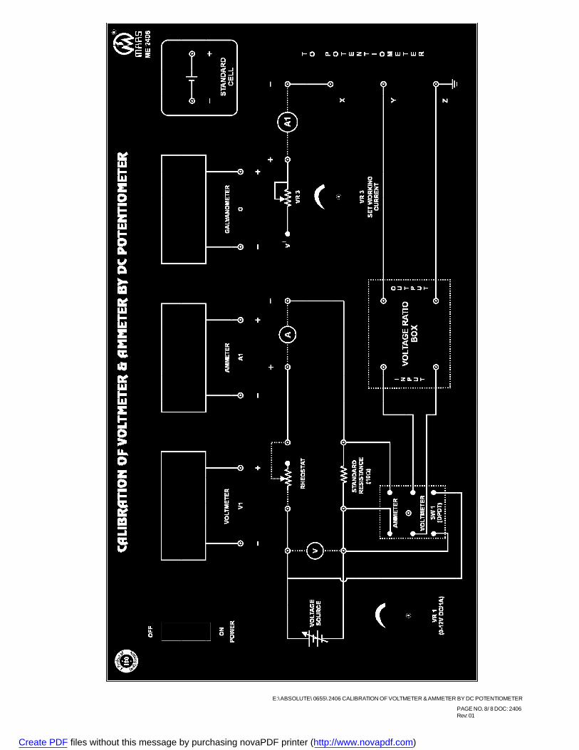
PAGE NO. 1/ 8 DOC: 2406Rev: 01
INSTRUCTION MANUALFOR
CALIBRATION OF VOLTMETR & AMMETER
BY DC POTENTIOMETER
MODEL NO. ME 2406
“Mars” made Calibration of Voltmeter & Ammeter by DC Potentiometer to study how to calibrate DC Voltmeter
& Ammeter using DC potentiometer for measurement.
The Experimental Setup consists of the following parts :
1. In built Power Supplies 0-12V DC/ 1A, 0-3V DC/ 200mA and 1V DC/ 200mA. For Current Source,
Voltage Source, Working Current Source and as Standard Cell respectively.
2. One number of Digital Panel Meter for current measurement i.e. A.
3. One number of Digital Panel Meter for voltage measurement i.e. V.
4. One number of Digital Panel Meter for galvanometer purpose i.e. G.
5. Circuit diagram on front panel with input and output sockets.
6. Voltage Ratio Box of range 300/ 150/ 30/ 15/ 1.5 ratio to 1.5.
7. DC Slide Wire Potentiometer of 10 columns. (Model No. ME 2224).
8. Rheostat of range 0 - 20 Ohms/ 1Amp.
9. One number Portable Analog DC Voltmeter 0 - 10V (Model No. 482), Separate.
10. One number Portable Analog DC Ammeter 0 - 1A (Model No. ME 486), Separate.
Create PDF files without this message by purchasing novaPDF printer (http://www.novapdf.com)
PAGE NO. 2/ 8 DOC: 2406Rev: 01
THEORY
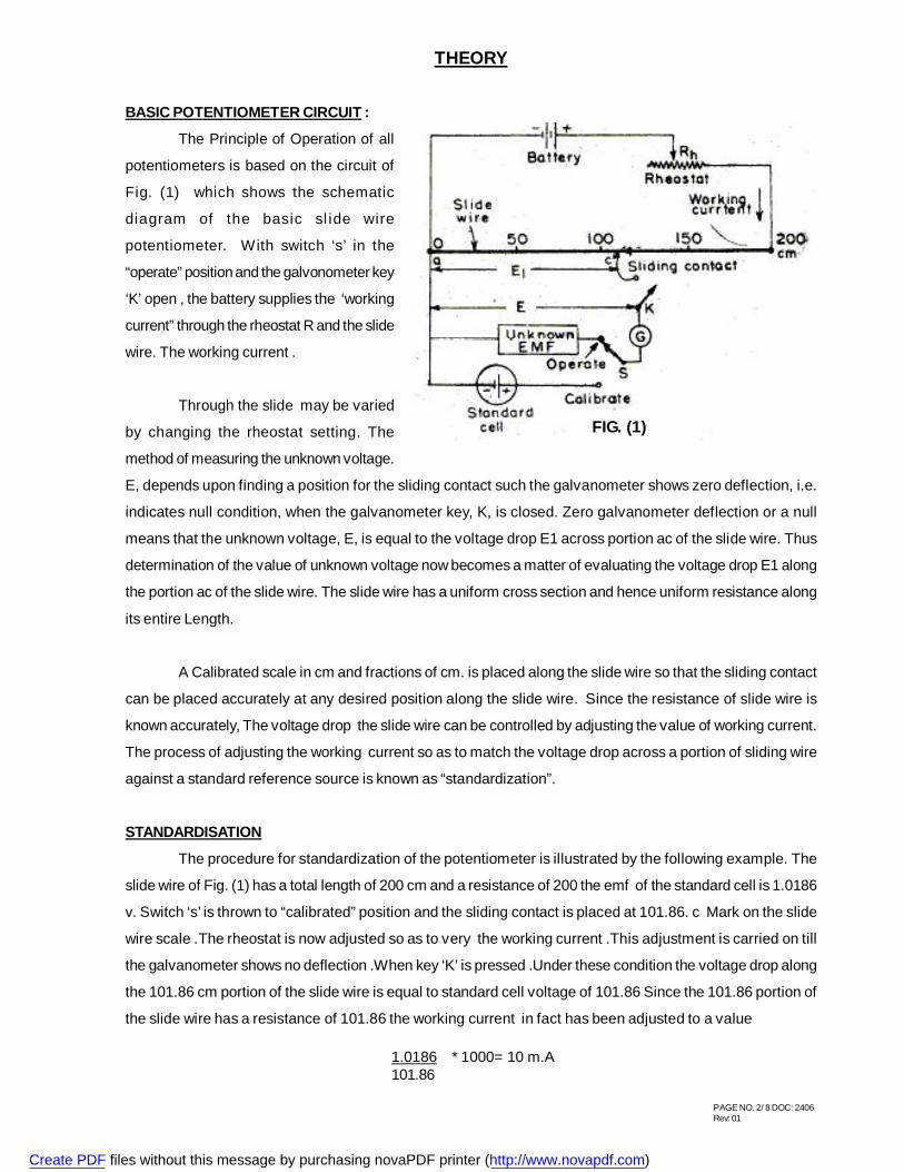
BASIC POTENTIOMETER CIRCUIT :
The Principle of Operation of all
potentiometers is based on the circuit of
Fig. (1) which shows the schematic
diagram of the basic sl ide wire
potentiometer. With switch ‘s’ in the
“operate” position and the galvonometer key
‘K’ open , the battery supplies the ‘working
current” through the rheostat R and the slide
wire. The working current .
Through the slide may be varied
by changing the rheostat setting. The
method of measuring the unknown voltage.
E, depends upon finding a position for the sliding contact such the galvanometer shows zero deflection, i.e.
indicates null condition, when the galvanometer key, K, is closed. Zero galvanometer deflection or a null
means that the unknown voltage, E, is equal to the voltage drop E1 across portion ac of the slide wire. Thus
determination of the value of unknown voltage now becomes a matter of evaluating the voltage drop E1 along
the portion ac of the slide wire. The slide wire has a uniform cross section and hence uniform resistance along
its entire Length.
A Calibrated scale in cm and fractions of cm. is placed along the slide wire so that the sliding contact
can be placed accurately at any desired position along the slide wire. Since the resistance of slide wire is
known accurately, The voltage drop the slide wire can be controlled by adjusting the value of working current.
The process of adjusting the working current so as to match the voltage drop across a portion of sliding wire
against a standard reference source is known as “standardization”.
STANDARDISATION
The procedure for standardization of the potentiometer is illustrated by the following example. The
slide wire of Fig. (1) has a total length of 200 cm and a resistance of 200 the emf of the standard cell is 1.0186
v. Switch ‘s’ is thrown to “calibrated” position and the sliding contact is placed at 101.86. c Mark on the slide
wire scale .The rheostat is now adjusted so as to very the working current .This adjustment is carried on till
the galvanometer shows no deflection .When key ‘K’ is pressed .Under these condition the voltage drop along
the 101.86 cm portion of the slide wire is equal to standard cell voltage of 101.86 Since the 101.86 portion of
the slide wire has a resistance of 101.86 the working current in fact has been adjusted to a value
1.0186 * 1000= 10 m.A101.86
FIG. (1)
Create PDF files without this message by purchasing novaPDF printer (http://www.novapdf.com)
PAGE NO. 3/ 8 DOC: 2406Rev: 01
The voltage at any point along the slide wire is proportional to the length of slide wire. This voltage is
obtained by converting the calibrated length into the corresponding the calibrated length into the corresponding
voltage simply by placing the decimal point in the proper position e.g. 153.6 cm = 1.536 V if the potentiometer
has been calibrated once its working current is never changed.
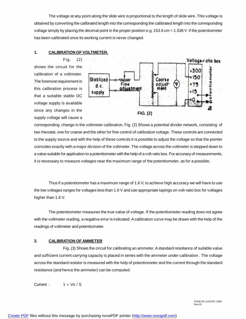
1. CALIBRATION OF VOLTMETER.
Fig. (2)
shows the circuit for the
calibration of a voltmeter.
The foremost requirement in
this calibration process is
that a suitable stable DC
voltage supply is available
since any changes in the
supply voltage will cause a
corresponding change in the voltmeter calibration. Fig. (2) Shows a potential divider network, consisting of
two rheostat, one for coarse and the other for fine control of calibration voltage. These controls are connected
to the supply source and with the help of these controls it is possible to adjust the voltage so that the pointer
coincides exactly with a major division of the voltmeter. The voltage across the voltmeter is stepped down to
a value suitable for application to a potentiometer with the help of a volt-ratio box. For accuracy of measurements,
it is necessary to measure voltages near the maximum range of the potentiometer, as for a possible.
Thus if a potentiometer has a maximum range of 1.6 V, to achieve high accuracy we will have to use
the low voltages ranges for voltages less than 1.6 V and use appropriate tapings on volt-ratio box for voltages
higher than 1.6 V.
The potentiometer measures the true value of voltage. If the potentiometer reading does not agree
with the voltmeter reading, a negative error is indicated. A calibration curve may be drawn with the help of the
readings of voltmeter and potentiometer.
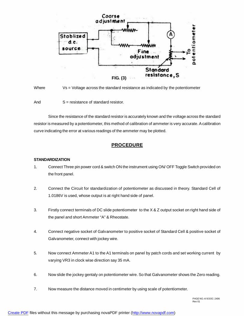
2. CALIBRATION OF AMMETER
Fig. (3) Shows the circuit for calibrating an ammeter. A standard resistance of suitable value
and sufficient current carrying capacity is placed in series with the ammeter under calibration . The voltage
across the standard resistor is measured with the help of potentiometer and the current through the standard
resistance (and hence the ammeter) can be computed.
Current : 1 = Vs / S
FIG. (2)
Create PDF files without this message by purchasing novaPDF printer (http://www.novapdf.com)
PAGE NO. 4/ 8 DOC: 2406Rev: 01
Where Vs = Voltage across the standard resistance as indicated by the potentiometer
And S = resistance of standard resistor.
Since the resistance of the standard resistor is accurately known and the voltage across the standard
resistor is measured by a potentiometer, this method of calibration of ammeter is very accurate. A calibration
curve indicating the error at various readings of the ammeter may be plotted.
PROCEDURE
STANDARDIZATION
1. Connect Three pin power cord & switch ON the instrument using ON/ OFF Toggle Switch provided on
the front panel.
2. Connect the Circuit for standardization of potentiometer as discussed in theory. Standard Cell of
1.0186V is used, whose output is at right hand side of panel.
3. Firstly connect terminals of DC slide potentiometer to the X & Z output socket on right hand side of
the panel and short Ammeter “A” & Rheostate.
4. Connect negative socket of Galvanometer to positive socket of Standard Cell & positive socket of
Galvanometer, connect with jockey wire.
5. Now connect Ammeter A1 to the A1 terminals on panel by patch cords and set working current by
varying VR3 in clock wise direction say 35 mA.
6. Now slide the jockey gentaly on potentiometer wire. So that Galvanometer shows the Zero reading.
7. Now measure the distance moved in centimeter by using scale of potentiometer.
FIG. (3)
Create PDF files without this message by purchasing novaPDF printer (http://www.novapdf.com)
PAGE NO. 5/ 8 DOC: 2406Rev: 01
8. Divide the 1.0186V into the distance moved in centimeters this will give you potential drop at 1cm of
wire or v/cm. let this be constant “C”.This is the calibration standard for whole experiment.
CALIBRATION OF VOLTMETER
9. Now also connect external analog voltmeter parallel with voltage source.
10. Also connect voltage ratio box to the panel in correct polarities.
11. Keep switch SW1 in voltmeter position i.e. down word .
12. Also set rated voltage across voltmeter, before setting rated voltage select the appropriate ratio of
voltage ratio box i.e. set to 15V : 1.5 V which give multification factor of 10. Let it be “M”.
13. You will see the full scale deflection in voltmeter.
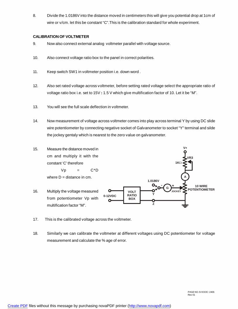
14. Now measurement of voltage across voltmeter comes into play across terminal Y by using DC slide
wire potentiometer by connecting negative socket of Galvanometer to socket “Y” terminal and silde
the jockey gentaly which is nearest to the zero value on galvanometer.
15. Measure the distance moved in
cm and multiply it with the
constant ‘C’ therefore
Vp = C*D
where D = distance in cm.
16. Multiply the voltage measured
from potentiometer Vp with
multification factor “M”.
17. This is the calibrated voltage across the voltmeter.
18. Similarly we can calibrate the voltmeter at different voltages using DC potentiometer for voltage
measurement and calculate the % age of error.
0-12VDCVOLT RATIOBOX
G
1.0186V
JOCKEY
Z
Y
- +
A
VR3
V+
10 WIREPOTENTIOMETER
1K
Create PDF files without this message by purchasing novaPDF printer (http://www.novapdf.com)
PAGE NO. 6/ 8 DOC: 2406Rev: 01
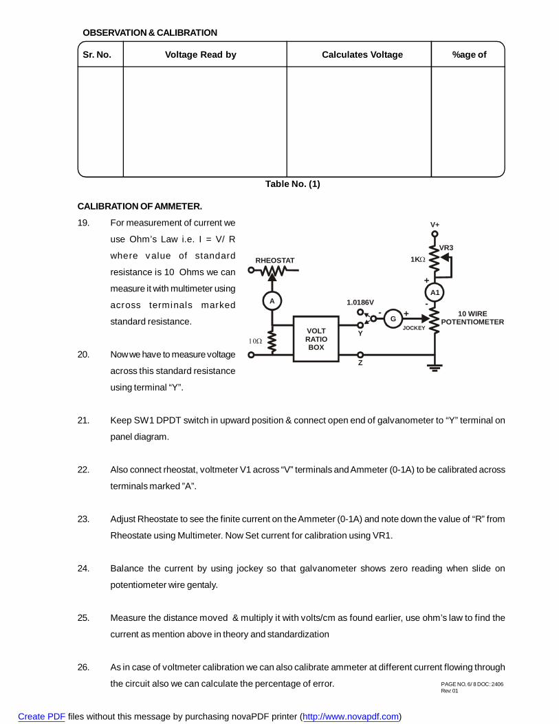
CALIBRATION OF AMMETER.
19. For measurement of current we
use Ohm’s Law i.e. I = V/ R
where v alue of standard
resistance is 10 Ohms we can
measure it with multimeter using
across terminals marked
standard resistance.
20. Now we have to measure voltage
across this standard resistance
using terminal “Y”.
21. Keep SW1 DPDT switch in upward position & connect open end of galvanometer to “Y” terminal on
panel diagram.
22. Also connect rheostat, voltmeter V1 across “V” terminals and Ammeter (0-1A) to be calibrated across
terminals marked ”A”.
23. Adjust Rheostate to see the finite current on the Ammeter (0-1A) and note down the value of “R” from
Rheostate using Multimeter. Now Set current for calibration using VR1.
24. Balance the current by using jockey so that galvanometer shows zero reading when slide on
potentiometer wire gentaly.
25. Measure the distance moved & multiply it with volts/cm as found earlier, use ohm’s law to find the
current as mention above in theory and standardization
26. As in case of voltmeter calibration we can also calibrate ammeter at different current flowing through
the circuit also we can calculate the percentage of error.
RHEOSTAT
VOLT RATIOBOX
G
A
JOCKEY
1.0186V
Z
Y
--
+
+A1
VR3
V+
10 WIREPOTENTIOMETER
1K
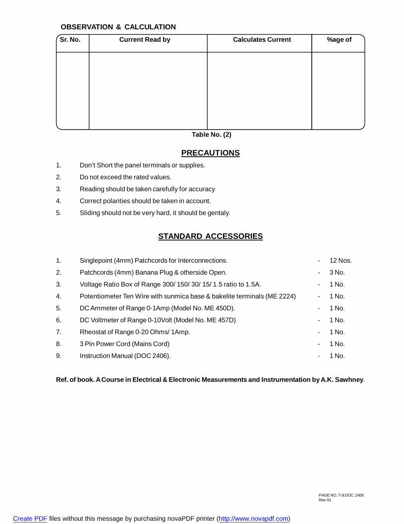
Table No. (1)
OBSERVATION & CALIBRATION
Sr. No. Voltage Read by Calculates Voltage %age of
Create PDF files without this message by purchasing novaPDF printer (http://www.novapdf.com)
PAGE NO. 7/ 8 DOC: 2406Rev: 01
PRECAUTIONS1. Don’t Short the panel terminals or supplies.
2. Do not exceed the rated values.
3. Reading should be taken carefully for accuracy
4. Correct polarities should be taken in account.
5. Sliding should not be very hard, it should be gentaly.
STANDARD ACCESSORIES
1. Singlepoint (4mm) Patchcords for Interconnections. - 12 Nos.
2. Patchcords (4mm) Banana Plug & otherside Open. - 3 No.
3. Voltage Ratio Box of Range 300/ 150/ 30/ 15/ 1.5 ratio to 1.5A. - 1 No.
4. Potentiometer Ten Wire with sunmica base & bakelite terminals (ME 2224) - 1 No.
5. DC Ammeter of Range 0-1Amp (Model No. ME 450D). - 1 No.
6. DC Voltmeter of Range 0-10Volt (Model No. ME 457D) - 1 No.
7. Rheostat of Range 0-20 Ohms/ 1Amp. - 1 No.
8. 3 Pin Power Cord (Mains Cord) - 1 No.
9. Instruction Manual (DOC 2406). - 1 No.
Ref. of book. A Course in Electrical & Electronic Measurements and Instrumentation by A.K. Sawhney.
Sr. No. Current Read by Calculates Current %age of
Table No. (2)
OBSERVATION & CALCULATION
Create PDF files without this message by purchasing novaPDF printer (http://www.novapdf.com)
PAGE NO. 8/ 8 DOC: 2406Rev: 01
E:\ ABSOLUTE\ 0655\ 2406 CALIBRATION OF VOLTMETER & AMMETER BY DC POTENTIOMETER
Create PDF files without this message by purchasing novaPDF printer (http://www.novapdf.com)

PAGE NO. 1/ 6 DOC 263REV. - 00
INSTRUCTION MANUALFOR
LCR - Q - METER (BRIDGE TYPE)
MODEL NO. ME 263
“MARS” made LCR Bridge has been designed to measure the value of Inductance, Capacitor & Resistance. The
bridge circuit are made up of high quality stable components to give accuracy for long period of use under varying
conditions. The RCL balancing dials use unique scale expansion device giving exception discrimination in reading.
The Instrument Comprises of the Following Build In Parts :
1. Five seprate bridges are assembled to form the LCR Bridge.
2. Built In Oscillator is provided in the instrument.
3. Built In Detector is provided in the instrument.
4. Selector switch is provided on the front panel for R, L & C.
5. Dials are provided on the front panel for D & Q.
The bridge is completely self contained and portable instrument. The five sperate bridge circuit are included
to give flexibility and wide range. Oscillator and null detector are built-in. The galvanometer indicates both AC & DC
bridge unbalances and therefore any external null detector or energizing source is not required.
Panel Description :
The panel carries RCL balancing dials, Range switch, RCL Function selector, Cp-Ls-Cs-Lp selector switch,
D & Q Dials, L & C sensitivity control, Galvanometer, switch for final balance, Terminal for connecting unknown
RCL & ON-OFF switch with indicator light. The function of each switch, control, dials etc. are explained as follows
:
Create PDF files without this message by purchasing novaPDF printer (http://www.novapdf.com)

PAGE NO. 2/ 6 DOC 263REV. - 00
Sr. No. Control/ Terminals Function
1. RCL BALANCING DIALS
(a) Coarse stepped switch calibrated 0 - 1 (a) Selects coarse steps & this give approx.
Null on the galvanometer.
(b) Continuous Vernier Calibrated 0 - 0.1 (b) Works as the vernier balance & ensure ease
of obtaining NULL as well as high degree of
reading discrimination.
2. Range Selector Switch Selects the required measuring range of LCR
Multiplier and the unit of measurement.
3. RCL Function Selector Selects the measuring function i.e. LCR.
4. Cp - Lp & Cs - Lp Switch Selects ten factor range of reactive components
being measured.
5. D & Q Dials Indicates D & Q of inductance & capacitor.
6. L & C Sensitivity Control Control the 1000 C/S unabalance signal
amplitude & thus controls the sensitivity on L
& C measurement.
7. Panel Meter Indicate balance of bridge circuit on
measurement of capacitor, indictance &
resistance.
8. LO - HI Terminals Are common terminals for connecting LCR to
be measured.
9. ON - OFF Switch & Indicator Light Puts the bridge ON or OFF, the light being ON
when the bridge is ON.
Create PDF files without this message by purchasing novaPDF printer (http://www.novapdf.com)
PAGE NO. 3/ 6 DOC 263REV. - 00
THEORY
The bridge employs five separate bridge circuits namely Wheatstone, De-sauty, Hay, Maxwell and Wein
Bridge.
Resistance :
Wheatstone bridge has been used for over a century for measurement of direct current resistance and is
considered the fundamental circuit for the purpose. It measures an unknown resistance in terms of calibrated
standards of resistance.
Capacitor :
De-Sauty Bridge may be considered as a wheatstone bridge circuit with two resistance arm & is used for
measuring capacitance in series with resistance i.e. Cs. This arrangement is obtained when the Cp-Ls/Cs-Lp
switch is in Cs-Lp position.
Wien Bridge :
When bridge is used for measurement of capacity is parallel with resistance and the arrangement is
obtained when the Cp-Ls and Cs-Lp switch is in Cp-Ls position.
Inductance (Maxwell Brige) :
This arrangement is used for the measurement of inductance having low Q & the arrangement is obtained
when Cp-Lp/Cs-Lp switch is in Cp-Ls position.
Hay Bridge :
Hay Bridge circuit arrangement is used to measure inductance and higher storage factor (Q) of indictance
and the arrangement is obtained when the Cp-Ls and Cs-Ls is in Cp-Ls position.
PROCEDURE
Resistance Measurement :
1. Connect resistance across HI, LO terminals. Set the selector switch at R marked on the front panel.
2. Switch ON the bridge. The Galvanometer will deflect right. Now adjust the balance dial to obtain a null, till
meter needle comes nearly to RED mark on the analog meter.
3. Select the proper range using range selector switch, which will show you sufficient deflection on meter.
Now variy the steps of coarse dial simultaneously with fine dial.
Create PDF files without this message by purchasing novaPDF printer (http://www.novapdf.com)
PAGE NO. 4/ 6 DOC 263REV. - 00
4. Repeat the steps until meter comes at nearly RED mark on the meter. Note down the range dial reading,
coarse dial reading and fine reading.
For Example :
Position of Range Switch = 10 K
Position of Balance Dial (Coarse) = 1
Position of Balance Dial (Vernier) = 0.05
R.X. = 10 Kx 1.05 = 10.5 K
Accuracy of Measurement :
The percentage error when measuring Resistace is +1% between 1ohms to 1 Megohms. The accuracy
falls at lower range to 5% at the highest. The measurement of Resistance is on AC source only.
Capacitance Measurement :
1. Connect the unknown capacitor to the LO-HI terminals keeping the connecting leads length as shorts as
possible. Care should also be taken to connect the output foil, Earth or Shield side of the capacitor to the
terminal marked LO.
2. Turn the final function selector to ‘C’.
3. Put the final balance switch in reverse position.
4. Advance the L & C sensitivity control so that deflection is obtained on the panel meter.
5. Turn the Cp-Ls and Cs-Lp switch in Cs-Lp position.
6. Switch ON the bridge, the meter will deflect to right.
7. Set D dial to minimum. Turn the range switch so that minimum deflection is obtained on the panel meter.
8. Adjust the balancing dials and D dial alternatively minimum deflection on the meter.
9. The value of capacitor is given by the balancing dial reading multiplied by the range selector reading. The
dissipation factor D is the indicated value on the D dial and needs no multiplier. D is the ratio of resistance
of reactance.
Create PDF files without this message by purchasing novaPDF printer (http://www.novapdf.com)
PAGE NO. 5/ 6 DOC 263REV. - 00
10. In case parallel capacitance is to be measured, the Cp-Ls and Cs-Lp switch is put in position Cp-Ls and
the bridge is now balanced by alternatly by adjustment of balancing dial and the Q dial.
Capacitor is read that as previous case.
Dissipation Factor (D) will not be the reciprocal of the reading indicated by the Q dial.
Parallel capacitance is found by using frequency in the megacycle range. Where leakage resistance loss
& lead inductance become appreciable.
Accuracy of Capacitor Measurement :
The percentage error of capacitance measurement is 1.5 percent (plus or minus 1/2 division) between
0.001F to 10F increase to 3 percent at the highest reading.
On small capacitance, the accuracy of measurment is again reduced and consideration must to made of
the internal capacitance of the bridge circuit and the capacitance of the leads wires connected to the unknown
capacitor proceed as following to determine the zero capacitance of the bridge
(a) Set the bridge controls to measure capacitance.
(b) Balance the bridge without using a capacitor between the LO-HI terminals.
(c) For measuring the leads wire capacitance, disconnect the leads wire at the capacitor and without changing
the spacing or relative position of the leads and balance the bridge.
Accuracy of the Dissipation Factor (D) Reading :
The accuracy of the dissipation factor reading is within 20 percent of 0.005 whichever is greater for capcitance
above 100F. This relatively large error occurs due to the reactance or the ratio arms which change with setting of
the range selector switch and the balancing dials.
Inductance Measurement :
a) Connect the unknown inductor to the LO-HI terminals keeping the connecting leads length as short as
possible. The shield, if any must be connected to the LO terminals.
b) Turn the Function selector to L. Set final balance switch in reverse position.
Create PDF files without this message by purchasing novaPDF printer (http://www.novapdf.com)
PAGE NO. 6/ 6 DOC 263REV. - 00
c) Advance the L & C sensitivity control so that deflection is obtained on the meter panel.
d) Turn the range switch so that minimum deflection is obtained on the meter panel.
e) Adjust the balancing dials and the D & Q dial (Depending on the position of the Cp-Ls and Cs-Lp switch)
alternatily to obtain minimum deflection on the panel meter. Position of Cp-Ls and Cs-Lp switch will depend
on the Q of the inductor under measurement. If the Q is lower than 10, balance would be obtained with Cp-
Ls and Cs-Lp position.
Note :
Series inductance (Ls) refers to the effective inductance of coil at the given frequency, when it is considered
to be in series with its residual resistance. Parallel inductance (Lp) refers to the effective inductance of a coil, at a
given frequency, when it is considered to be shunted by the resistance of the coil.
Storage Factor of an Inductor :
After balance has been obtained as explanied above, the Q of the inductor will be reading of Q Dial (Cp-Ls
and Cs-Lp) switch being in Cs-Lp). The Q of the inductor is the ratio of reactance to resistance.
Thus it is the reciprocal of the dissipation factor D. The series AC Resistance of the inductor under
measurement may be calculated from the following formula : When balance is obtained Cp-Ls/Cs-Lp switch is in
Cs-Lp position. The Q is reciprocal of the reading of D dial.
STANDARD ACCESSORIES
1. Two Patchcords one side banana plug & other side crocodial clip.
2. Instruction Manual (DOC 263).
Create PDF files without this message by purchasing novaPDF printer (http://www.novapdf.com)
PAGE NO. 1/ 3 DOC 546REV. : 02
INSTRUCTION MANUALFOR
THERMISTOR CHARACTERISTICS APPARATUS
MODEL NO. ME 546, 546D & P
'MARS' made Thermistor Characteristics Apparatus has been designed to plot.
1. Temperature Vs Resistance characteristics at different Voltage.
2. Voltage Vs Current characteristics at different Temperatures.
3. Current Vs Time characteristic at different Voltages.
The Instrument comprises of the following built in parts:-
1. Continuously variable, overload & short circuit protected DC Regulated power supply of 0-10 Volt.
Input Voltage : 230 V +10% AC, 50 Hz
Load Regulation : + 0.2%
Line Regulation : + 0.05%
Ripple : Less than 3 mV R.M.S.
Protections : Against Short Circuit & Over Load
2. Two meters to measure voltage & current are mounted on front panel & connections brought out on 4mm
Sockets.
3. Mercury Thermometer is also mounted on the front panel to read the different temperature readings of the
oven.
4. 68KGlass Thermistor is mounted inside the oven.
THEORY
The Thermistor is a thermally sensitive resistance, the temperature coefficient of which is large and negative. They
are essentially semiconductors which behaves as resistors with a very high negative temperature coefficient of
resistance. For many years thermistors are basically used in temperature compensate circuits.
Create PDF files without this message by purchasing novaPDF printer (http://www.novapdf.com)
PAGE NO. 2/ 3 DOC 546REV. : 02
PROCEDURE
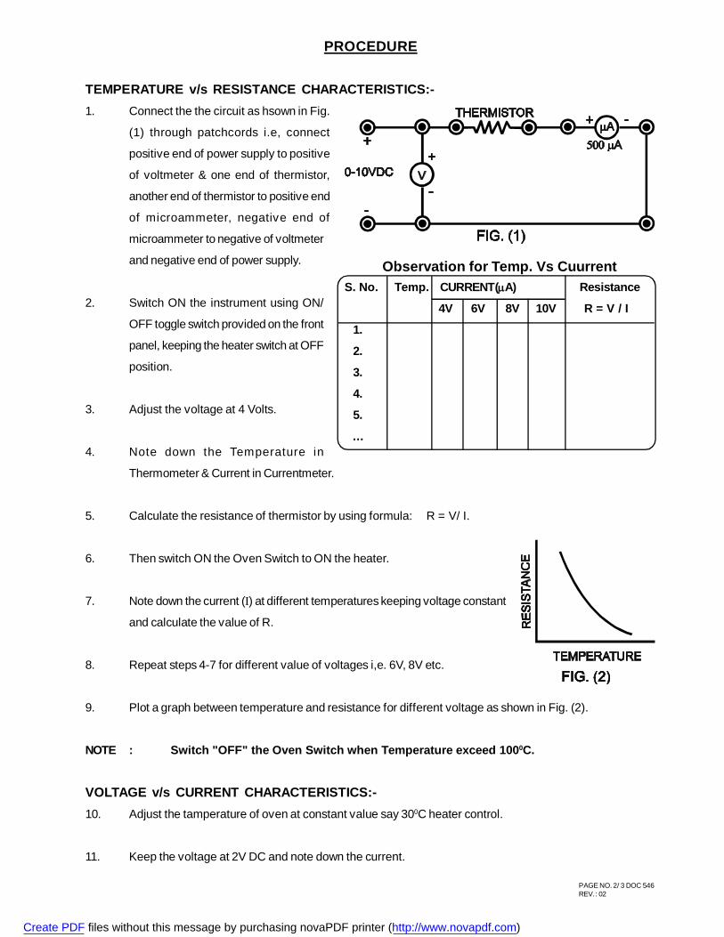
TEMPERATURE v/s RESISTANCE CHARACTERISTICS:-1. Connect the the circuit as hsown in Fig.
(1) through patchcords i.e, connect
positive end of power supply to positive
of voltmeter & one end of thermistor,
another end of thermistor to positive end
of microammeter, negative end of
microammeter to negative of voltmeter
and negative end of power supply.
2. Switch ON the instrument using ON/
OFF toggle switch provided on the front
panel, keeping the heater switch at OFF
position.
3. Adjust the voltage at 4 Volts.
4. Note down the Temperature in
Thermometer & Current in Currentmeter.
5. Calculate the resistance of thermistor by using formula: R = V/ I.
6. Then switch ON the Oven Switch to ON the heater.
7. Note down the current (I) at different temperatures keeping voltage constant
and calculate the value of R.
8. Repeat steps 4-7 for different value of voltages i,e. 6V, 8V etc.
9. Plot a graph between temperature and resistance for different voltage as shown in Fig. (2).
NOTE : Switch "OFF" the Oven Switch when Temperature exceed 1000C.
VOLTAGE v/s CURRENT CHARACTERISTICS:-10. Adjust the tamperature of oven at constant value say 300C heater control.
11. Keep the voltage at 2V DC and note down the current.
Observation for Temp. Vs CuurrentS. No. Temp. CURRENT(A) Resistance
4V 6V 8V 10V R = V / I
1.
2.
3.
4.
5.
...
Create PDF files without this message by purchasing novaPDF printer (http://www.novapdf.com)
PAGE NO. 3/ 3 DOC 546REV. : 02
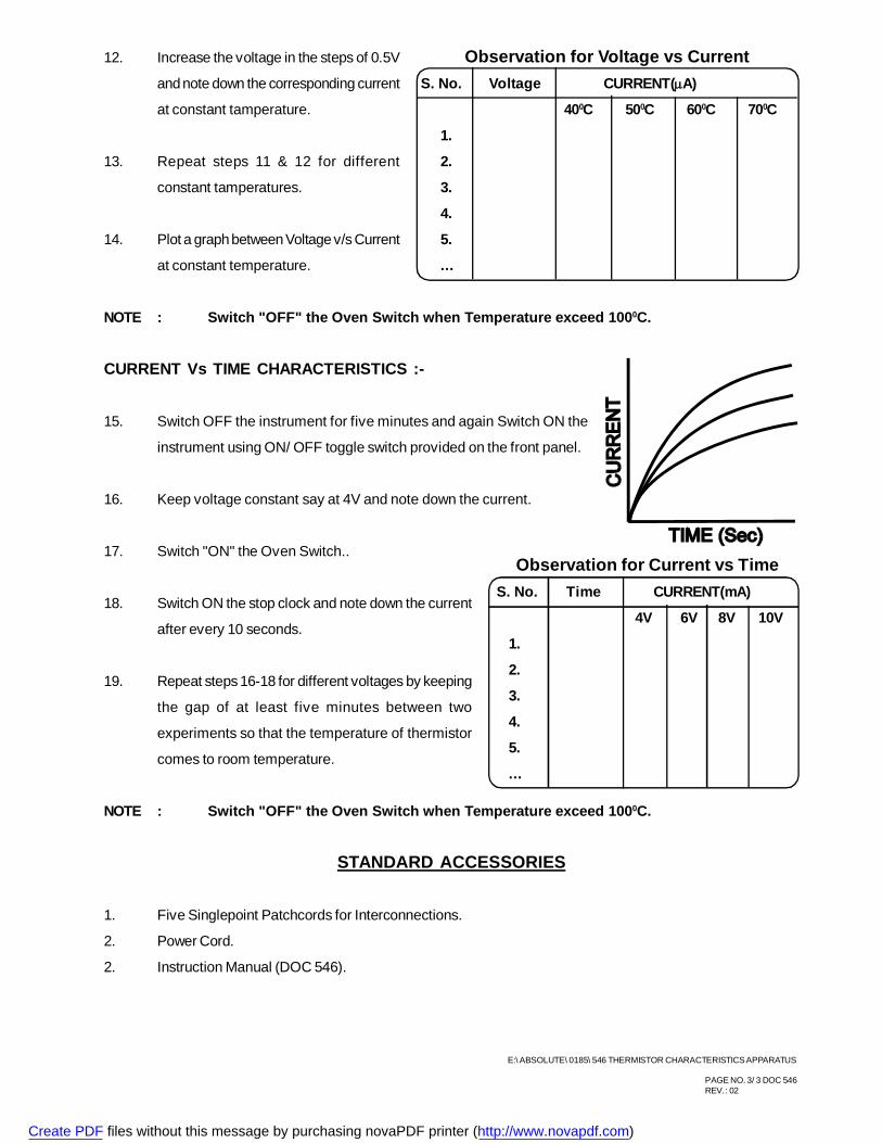
12. Increase the voltage in the steps of 0.5V
and note down the corresponding current
at constant tamperature.
13. Repeat steps 11 & 12 for different
constant tamperatures.
14. Plot a graph between Voltage v/s Current
at constant temperature.
NOTE : Switch "OFF" the Oven Switch when Temperature exceed 1000C.
CURRENT Vs TIME CHARACTERISTICS :-
15. Switch OFF the instrument for five minutes and again Switch ON the
instrument using ON/ OFF toggle switch provided on the front panel.
16. Keep voltage constant say at 4V and note down the current.
17. Switch "ON" the Oven Switch..
18. Switch ON the stop clock and note down the current
after every 10 seconds.
19. Repeat steps 16-18 for different voltages by keeping
the gap of at least five minutes between two
experiments so that the temperature of thermistor
comes to room temperature.
NOTE : Switch "OFF" the Oven Switch when Temperature exceed 1000C.
STANDARD ACCESSORIES
1. Five Singlepoint Patchcords for Interconnections.
2. Power Cord.
2. Instruction Manual (DOC 546).
Observation for Current vs TimeS. No. Time CURRENT(mA)
4V 6V 8V 10V
1.
2.
3.
4.
5.
...
Observation for Voltage vs CurrentS. No. Voltage CURRENT(A)
400C 500C 600C 700C
1.
2.
3.
4.
5.
...
E:\ ABSOLUTE\ 0185\ 546 THERMISTOR CHARACTERISTICS APPARATUS
Create PDF files without this message by purchasing novaPDF printer (http://www.novapdf.com)
PAGE NO. 1\ 4 DOC 552REV. - 01
INSTRUCTION MANUAL
FOR
TRIAC CHARACTERISTICS APPARATUS
MODEL NO. ME 552
‘MARS’ made Triac Characteristics Apparatus has been designed to plot the V-I characteristics of a Triac.
The instrument comprises of the following built in parts :
1. Two continuously variable overload & short circuit protected DC regulated power supplies of 0-3V for Gate
Current and 0-30V for MT1 & MT2 are provided in ME 552, ME 552D & ME 552P.
Input Voltage : 230 V +10% AC, 50 Hz
Load Regulation : + 0.2%
Line Regulation : + 0.05%
Ripple : Less than 3 mV R.M.S.
Protections : Against Short Circuit & Over Load
2. Three meters to measure voltage & current are mounted on front panel & connections brought out on Sockets.
3. Triac (BT136) is mounted inside the cabinet and pin connections are brought out at terminals/ sockets.
THEORY
The major drawback of an SCRis that it can conduct current in one direction only. Therefore, an SCR can only
control DC power or forward biased half-cycles of AC in a load. However, in an AC system, it is often desirable and
necessary to exercise control over both positive and negative half-cycles. For this purpose, a semiconductor device
called Triac is used.
A Triac is a three terminals semiconductor switching device which can control alternating current in a load.
‘Triac is an abbreviation for triode AC switch. ‘Tri’ - indicates that the device has three terminals and AC
means that the device controls alternating current or can conduct current in either direction. Since a triac can
control conduction of both positive & negative half-cycles of AC supply, it is sometimes called a bidirectional semi-
conductor triode switch. A triac is a bidirectional switch having three terminals. It can be seen that even symbol of
triac indicates that it can conduct for either polarity of voltage across the main terminals. The gate provides control
Create PDF files without this message by purchasing novaPDF printer (http://www.novapdf.com)
PAGE NO. 2\ 4 DOC 552REV. - 01
over conduction in either direction. Triacs are commercially available to handle maximum r.m.s. currents from about
0.5A upto 25A, although special triacs for upto about 1000 A have been developed. As the current handling capacity
increases so does the semi-conductor element size and the containing package.
PROCEDURE
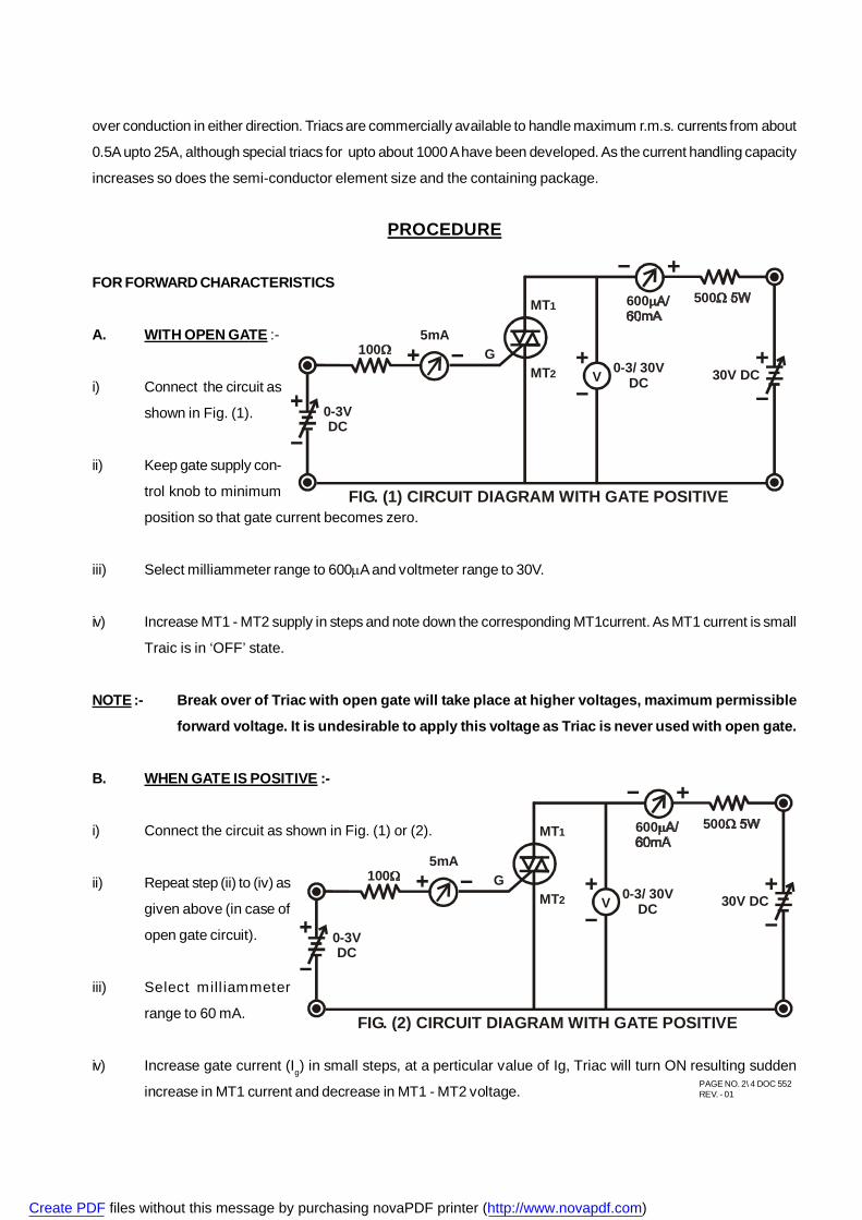
FOR FORWARD CHARACTERISTICS
A. WITH OPEN GATE :-
i) Connect the circuit as
shown in Fig. (1).
ii) Keep gate supply con-
trol knob to minimum
position so that gate current becomes zero.
iii) Select milliammeter range to 600A and voltmeter range to 30V.
iv) Increase MT1 - MT2 supply in steps and note down the corresponding MT1current. As MT1 current is small
Traic is in ‘OFF’ state.
NOTE :- Break over of Triac with open gate will take place at higher voltages, maximum permissible
forward voltage. It is undesirable to apply this voltage as Triac is never used with open gate.
B. WHEN GATE IS POSITIVE :-
i) Connect the circuit as shown in Fig. (1) or (2).
ii) Repeat step (ii) to (iv) as
given above (in case of
open gate circuit).
iii) Select mill iammeter
range to 60 mA.
iv) Increase gate current (Ig) in small steps, at a perticular value of Ig, Triac will turn ON resulting sudden
increase in MT1 current and decrease in MT1 - MT2 voltage.
FIG. (1) CIRCUIT DIAGRAM WITH GATE POSITIVE
V
0-3VDC
0-3/ 30VDC
MT1
GMT2 30V DC
1005mA
500600
FIG. (2) CIRCUIT DIAGRAM WITH GATE POSITIVE
V
0-3VDC
0-3/ 30VDC
MT1
GMT2 30V DC
1005mA
500600
Create PDF files without this message by purchasing novaPDF printer (http://www.novapdf.com)
PAGE NO. 3\ 4 DOC 552REV. - 01
v) Change the range of voltmeter to 3V after triggering of Triac.
vi) Also note the gate current Ig required for triggering the Triac at a given VMT1 - MT2.
vii) Record different breakover voltages and triggering gate currents.Plot the graph as shown in the Fig. No. (4).
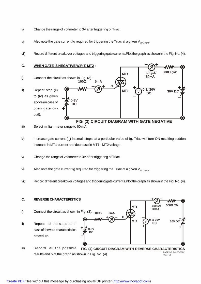
C. WHEN GATE IS NEGATIVE W.R.T. MT2 :-
i) Connect the circuit as shown in Fig. (3).
ii) Repeat step (ii)
to (iv) as given
above (in case of
open gate cir-
cuit).
iii) Select milliammeter range to 60 mA.
iv) Increase gate current (Ig) in small steps, at a perticular value of Ig, Triac will turn ON resulting sudden
increase in MT1 current and decrease in MT1 - MT2 voltage.
v) Change the range of voltmeter to 3V after triggering of Triac.
vi) Also note the gate current Ig required for triggering the Triac at a given VMT1 - MT2.
vii) Record different breakover voltages and triggering gate currents.Plot the graph as shown in the Fig. No. (4).
C. REVERSE CHARACTERISTICS
i) Connect the circuit as shown in Fig. (3).
ii) Repeat all the steps as in
case of forward characteristics
procedure.
iii) Record al l the possible
results and plot the graph as shown in Fig. No. (4).
FIG. (3) CIRCUIT DIAGRAM WITH GATE NEGATIVE
V
0-3VDC
0-3/ 30VDC
MT1
GMT2 30V DC
100 5mA
500600
FIG. (4) CIRCUIT DIAGRAM WITH REVERSE CHARACTERISTICS
V
0-3VDC
0-3/ 30VDC
MT1
GMT2 30V DC
100 5mA
500600
Create PDF files without this message by purchasing novaPDF printer (http://www.novapdf.com)
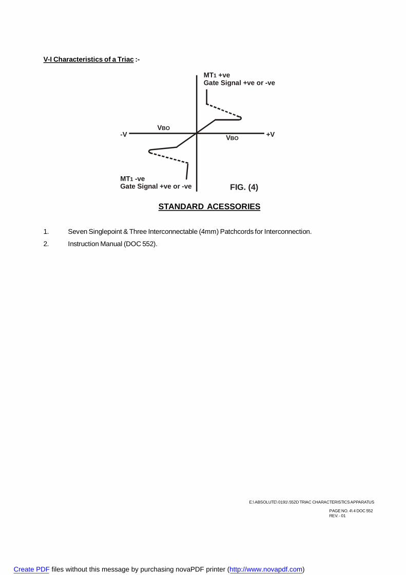
PAGE NO. 4\ 4 DOC 552REV. - 01
VBO
VBO
MT -veGate Signal +ve or -ve
1
MT +veGate Signal +ve or -ve
1
-V +V
FIG. (4)
E:\ ABSOLUTE\ 0191\ 552D TRIAC CHARACTERISTICS APPARATUS
V-I Characteristics of a Triac :-
STANDARD ACESSORIES
1. Seven Singlepoint & Three Interconnectable (4mm) Patchcords for Interconnection.
2. Instruction Manual (DOC 552).
Create PDF files without this message by purchasing novaPDF printer (http://www.novapdf.com)