Embed Size (px)
Citation preview


1
Institut Wohnen und Umwelt GmbH
Institute for Housing and Environment
Rheinstraße 65
D-64295 Darmstadt
www.iwu.de
Authors:
Andreas Enseling
Tobias Loga
T: +49-6151-2904-55
BPIE editing and reviewing team:
Bogdan Atanasiu
Ilektra Kouloumpi
Ingeborg Nolte
Marine Faber
Cosmina Marian

2
Table of Contents
1 Introduction ...............................................................................................................3
1.1 Aim of the study ..........................................................................................................3
1.2 Results of the global cost calculation ..........................................................................3
1.3 Remarks .....................................................................................................................4
2 Cost-optimal methodology for new buildings ........................................................8
2.1 Overview .....................................................................................................................8
2.2 Reference buildings .................................................................................................. 10
2.3 Selection of variants ................................................................................................. 13
2.4 Energy performance assessment.............................................................................. 16
2.5 Global cost calculation .............................................................................................. 17
3 Cost-optimal levels for new buildings ................................................................... 21
3.1 Private financial perspective ..................................................................................... 21
3.2 Macroeconomic perspective ..................................................................................... 28
3.3 Sensitivity analysis .................................................................................................... 31
References .......................................................................................................................... 37
Annex 1: Initial investment costs ...................................................................................... 39
Annex 2: Reporting table for energy performance relevant data .................................... 41
Annex 3: Global cost calculation – output data ............................................................... 43
Annex 4: Sensitivity analysis – output data ..................................................................... 48
Annex 5: Energy performance – output data.................................................................... 57

3
1 Introduction
1.1 Aim of the study
Directive 2010/31/EU on the energy performance of buildings (recast) stipulates that Member
States shall ensure that minimum energy performance requirements are set with a view to
achieving at least cost-optimal levels for buildings, building units and building elements. To
determine the cost-optimal levels, Member States are required to use a comparative
framework methodology (cost-optimal methodology) established by the Commission and
complete this framework with the relevant national parameters.
BPIE is implementing a study for providing more guidance and good practices for a proper
implementation of the EPBD cost-optimality requirement within the EU Member States. The
study is based on a detailed analysis of the cost-optimality approach in some selected EU
Member States with the aim of:
Proposing guidance on how to properly deal with several influential factors
Sharing lessons learned;
Analysing the influence of using a more realistic societal discount rate and more
ambitious simulation variants/packages;
Identifying the gap between cost-optimal and nearly zero-energy levels.
On behalf of BPIE IWU has carried out a study on cost-optimal levels for new residential
buildings following the cost-optimal methodology for Germany. The methodological basis,
the measures and the costs were developed in the framework of the project: "Evaluation and
Further Development of EnEV 2009: Study about the Economic Framework Conditions in
Housing“ on behalf of the Federal Institute for Research on Building, Urban Affairs and
Spatial Development [IWU 2012].
1.2 Results of the global cost calculation
From a private financial perspective the calculated cost-optimal primary energy values of
new buildings are approximately 53 kWh/m²a for the selected multi-family building (MFH) and
54 kWh/m²a for the selected single-family building (SFH). The cost optimal levels are not yet
reached by the current requirements (EnEV 2009). The minimum energy performance
requirements could be tightened by about 15 % to achieve cost-optimal levels and by about
25 % to achieve the same global costs as EnEV 2009. However, this gap will be closed by
an EnEV recast drafted by the German government: The maximum primary energy demand
shall be lowered in two steps, each time by 12.5%.

4
In the most cost-effective cases higher energy performance standards towards nZEB (e.g.
“efficiency building 55” and “efficiency building 40”1) will involve increases of additional global
costs between 23 €/m² and 101 €/m² compared to EnEV 2009.
The calculations from a macroeconomic perspective (without VAT and with cost of
greenhouse gas emissions) show that the cost-optimal levels do not change compared to the
private financial perspective (cost-optimal level 54 kWh/(m²a) for SFH and 53 kWh/(m²a) for
MFH. Only the additional costs of advanced energy performance standards compared to
EnEV 2009 are decreasing. From a macroeconomic perspective the “efficiency building 55”
and “efficiency building 40” will involve increases of additional global costs compared to
EnEV 2009 between 13 €/m² and 77 €/m² in the most cost-effective cases.
1.3 Remarks
An important influential factor for the cost-optimal methodology is the selection of input
factors. The sensitivity analysis shows that changes of one input factor (discount rate, energy
price development) have a certain influence on the results compared to the standards
assumptions of the basic scenario. Lower discount rates and a higher energy price
development are leading to lower cost-optimal primary energy values, therefore the gap to
current requirements is becoming bigger and the additional costs of higher energy
performance standards compared to EnEV 09 are decreasing. Higher energy performance
standards are becoming more profitable or less non-profitable depending on the standard.
The influence on the results is really significant if two input factors are changed
simultaneously and are taking effect in the same direction e.g. a combination of a discount
rate of 1 % and a high energy price development. In the frame of the cost-optimal
methodology the choice of input factors is an important influential factor and should be
established with care.
Other important factors for the cost-optimal levels are the initial investment costs. In contrast
to existing buildings [Hinz 2010] empirically verified studies based on invoiced investment
costs of energy savings measures for new buildings are currently not available for Germany.
Within the project ‘Evaluation and Further Development of EnEV 2009: Study about the
Economic Framework Conditions in Housing’ [IWU 2012] three architecture and engineering
offices were commissioned to investigate costs for different levels of insulation and different
types of heat supply systems based on actual cost statements and tenders of recent
construction projects. Each office developed detailed scenarios for the given model buildings
and analysed how to implement the different levels of energy performance for the different
techniques. On this basis the costs were projected (similar to the standard planning process)
by considering all relevant elements and devices. The resulting cost data were analysed and
1 Funded energy performance standards of the German promotional bank KfW

5
averaged by IWU to determine cost functions, facilitating an easy variation of insulation
thickness and building size during the economical assessment.
An alternative method to determine the costs of different energy performance standards
would be to make a broad market research on new built homes in Germany. The problem is
only that the energy quality of a building correlates also with other building features. For
example, it may be that energy efficient buildings like passive houses are currently
constructed mainly by financially strong owners. Of course, it can be assumed that these
owners also install premium bathrooms, kitchens and garages or appreciate prestigious
façade surfaces or roof tiles. The incremental costs of insulation could only be determined if
the other price determining features were also elevated. Such a comprehensive
representative survey does not yet exist in Germany. But even if it could be implemented, the
question of accuracy has to be answered: Is the number of new buildings sufficiently large to
determine the – compared to other features – small influence of the energy performance on
the construction costs (or market price)?
Another influential factor is the reference building selection. In recent studies some
adaptations of the “official” building data had to be done by IWU in collaboration with the
three involved architect offices in order to define realistic planning scenarios. For the future
we recommend to use model buildings designed by architects. The buildings should have
rather common and simple geometries and the realisation should in principle be practicable –
for all considered energy performance levels. Designs which do not take account of the basic
principles of energy efficient architecture and which are not favourable to attain nZEBs
should be excluded. Furthermore, plans of actually built houses could be used - with
simplifications or adaptations, if necessary.
The basis of the cost optimum analysis is the energy balance calculation according to the
national implementation of EPBD. The energy performance calculation includes standard
assumptions of climatic conditions and user behaviour. These boundary conditions are not
necessarily identical with typical or average values of the country. For example, the German
asset rating calculation (EnEV 2009 / DIN V 4108-6) is based on a set-point temperature of
19°C. However, there is evidence that significantly higher temperatures can be typically
found in well insulated buildings and significantly lower in poorly insulated buildings (new
buildings: 20-21°C, existing not refurbished buildings: 17°C). Since the economic
assessment of insulation depends on the assumed room temperature, it should be discussed
if this effect should be considered in the C-O calculations. The inclusion of this effect could
lead to two different results: a) the assumption of a higher room temperature level for new
buildings would presumably result in an improved cost effectiveness of thermal protection in
this case and b) assuming realistic room temperatures for non-refurbished old buildings
would lead to lower (more realistic) energy savings and a decreasing cost effectiveness of
insulation measures.
The discussion of reality based assumptions may in the future also include other boundary
conditions, e.g. the shading by buildings or trees nearby (the standard assumption in the

6
German regulation doesn’t consider shading), the air exchange rates with and without
ventilation system etc.
The economic analyses of exemplary new buildings in this study were carried out by
assuming a distinct construction system. The considered buildings have masonry walls with
an external insulated render system, the ceilings are assumed as concrete elements. The
pitched roof of the semi-detached house is a wooden construction whereas the flat roof of
the multi-family house is a concrete structure with insulation on the top [IWU 2012].
Of course, in practice, further construction systems can be found, but due to the correlation
with other non-energy related costs and the associated uncertainties (see chapter 2.5) we
can say that the determination of cost optima only makes sense within a given construction
system but not between different types.
An official definition of nZEBs has not yet been published in Germany. Nevertheless, we can
assume that the definition will be close to the standard "KfW Effizienzhaus 40" (“efficiency
building 40”, primary energy demand = 40% of the requirements), which is the most
ambitious level of the Federal grant programme for new buildings. Already now the standard
“Effizienzhaus 40” was used in scenario calculations for the German building stock as an
equivalent of the not yet exactly defined nZEB standard of new buildings for the 2020
projection. To fill the gap between the current requirements of EnEV 2009 and this nZEB
level, a step by step tightening of the requirements as it is drafted in Germany seems to be
the right way ahead.
Compared to typical construction costs for new buildings in Germany (1300 €/m²) the
additional global costs for the most cost-effective standards towards nZEB range between 2
% and 8 %. These percentages are in a similar range as “typical fluctuations" of construction
costs. Nevertheless, a tightening of the minimum energy performance requirements from
EnEV 09 or from the cost-optimal level towards nZEB would be non-economical. This is in
line with the EPBD but would cause problems with the German energy saving law
(Energieeinsparungsgesetz EnEG), which postulates that minimum energy performance
requirements have to be "economically justifiable". This is an obstacle for the implementation
of the EPBD requirements to introduce nZEB levels for new buildings in 2020. After the
planned tightening of requirements further improvements will be non-economic and therefore
not justifiable against the German energy saving law.
By the use of the ‘cost-optimal methodology’ it is remarkable that as a result of the given
flexibility (e.g. selection of reference buildings, optional discount rates, selection of variants)
on the one hand and the fixed input factors and sensitivity analysis on the other hand, a great
number of cost-optimal levels or cost-optimal ranges occurs. In this context it seems to be a
big challenge to avoid another “painful” reporting exercise for the Member States.
Regarding the macroeconomic perspective, it can be stated that the considered costs of
greenhouse gas emissions respective the assumed carbon prices from Annex II of the C-O

7
regulation are too low to cause relevant changes in cost-optimal levels. For relevant changes
in cost-optimal levels, the assumed carbon prices must be clearly higher.
There are some studies available about the internalization of external environmental costs in
the construction sector [e.g.BMVBS 2010] but the investigation of external costs in
construction requires still a lot of research. As long as the German energy saving law
(Energieeinsparungsgesetz EnEG) postulates that minimum energy performance
requirements have to be "economically justifiable", it is obvious that the private financial
perspective for private investors may be seen as an appropriate basis for official cost-optimal
calculations.

8
2 Cost-optimal methodology for new buildings
2.1 Overview
The cost-optimal methodology defines for Member States the following procedure to
determine cost-optimal levels for new residential buildings2:
1. Definition of reference buildings
2. Selection of variants
3. Energy performance assessment
4. Global cost calculation
5. Sensitivity analysis
6. Determination of cost optimal levels
For the global cost calculation some input factors are fixed (e.g. calculation period, cost
categories, starting year of the calculation, use of a discount rate of 3 %), some other have to
be defined on national level (e.g. energy prices, energy price development, lifetime of
buildings and building components, use of disposal costs)
The following table shows the main assumptions and input factors for the cost-optimality
calculation from a private financial perspective (new buildings). The single input factors and
assumptions were described in more detail within chapters 2.2 to 2.5.
2 See Annex I [EC 2012a]

9
Table 1: Assumptions and input factors for the cost-optimality study in Germany (private financial perspective)
Assumptions and input factors cost-optimality study Germany (private financial perspective)
Reference buildings New residential buildings: 1 SFH; 1 MFH
Measures/variants/packages Packages: Combinations of thermal protection and heat supply system
Energy performance assessment DIN V 4108-6 together with DIN V 4701-10 – version valid for EnEV 2009 (new
buildings)
Cost categories
Investment cost
Residual value
Replacement cost
Maintenance cost
Energy cost
Calculation Method
Global cost calculation - net present value method
Calculation with real terms (inflation-adjusted)
Lifetime of building components 50 years (thermal protection) / 30 years (windows) / 15 years (technical
installations) according to DIN 15459 Annex A
Calculation period 30 years
Inflation 2 %/a (long-term goal ECB)
Discount rate 3.0 % (basic scenario) / 1 %
Price development for maintenance and replacement 0 %/a
Annual cost for maintenance (for technical installations) 2 % of initial investment costs
Current energy prices 7.0 Cent/kWh (gas), 5.0 Cent/kWh (wood pellets), 25.0 Cent/kWh (electricity
auxiliary energy), 19.0 Cent/kWh (special tariff heat pump)
Energy price development
Low: 1.3 %/a
Medium: 2.8 %/a (basic scenario)
High: 4.3 %/a

10
2.2 Reference buildings
An exemplary single-family building (semi-detached house) and one multifamily building are
considered as reference buildings. The used building data were developed in [ZUB 2010] on
behalf of the Federal Ministry of Transport, Building and Urban Development (BMVBS) with
the intention to provide reference buildings for the economical assessment of legal
requirements. The buildings were used as model buildings in the study [IWU 2012] on behalf
of BMVBS which is also the basis for the present investigation.
In this context some adaptations of the building data had to be done by IWU in collaboration
with the three involved architect offices. The main changes were (for details see [IWU 2012]):
Single-family house / semi-detached building:
Rotation by 90° to enable the installation of solar collectors (also corrected in the building
picture);
Inclusion of the top attic space in the thermal envelope: avoids problems with tightness
and thermal bridging, provides a room for installation of heating and ventilation system –
and is normal in new buildings (also corrected in the building picture);
Lowering of the ground level below cellar ceiling: so the render insulation system can
extend below the bottom edge of the cellar ceiling (standard solution);
Cellar access is outside the thermal envelope: helps avoiding thermal bridging.
Multi-family house / apartment building:
No neighbour building in the South: otherwise the thermal area of the walls would have
been extremely small and also the costs would have been not representative due to the
very high window fraction (also corrected in the building picture);
Balconies are realised as detached static structures: avoidance of thermal bridging;
Cellar access is outside the thermal envelope: helps avoiding thermal bridging.

11
The basic data of the model buildings are:
1. Single-family building (SFH) Heated volume Ve: 586 m³ Heated living space: 139 m² Usefull floor area AN acc. to EnEV: 187.5 m² Surface area S: 344.5 m² S/Ve: 0.59 m-1
Picture: [ZUB 2010], modified by IWU
2. Multifamily building (MFH) Heated volume Ve: 1848 m³ Heated living space: 473,0 m² Useful floor area AN acc. to EnEV: 591.4 m² Surface area S: 776.0 m² S/Ve: 0.42 m-1
Picture: [ZUB 2010], modified by IWU
The thermal envelope of the model buildings had been defined without designing the interior
of the buildings [ZUB 2010]. From our point of view this leads to a number of disadvantages.
For example, the multi-family building has 12 apartments with a total living area of
(estimated) 473 m² resulting in apartment sizes about 40 m² which is rather small. One
consequence is rather high costs per m² for individual ventilation systems installed in the
different apartments.

12
The publication of the two buildings included a table with the basic data and all thermal
envelope areas as well as perspective drawings [ZUB 2010]. This turned out to not be
sufficient for the architect offices to determine the costs of the different measure variants.
They would have needed at least ground plans and façade views with dimensions, to
determine specific lengths or areas (sizes of single windows, edge lengths of the roof areas
and the facades …). So they had to make individual assumptions which may differ in some
points.
In the future we recommend using model buildings designed by architects. The buildings
should have rather common and simple geometries; the realisation should in principle be
practicable. Also plans of actually built houses could be used - with simplifications or
adaptations, if necessary.3
3 Three examples of such real model buildings "re-designed" by an architect to fit the task can be found in: Loga, Tobias; Knissel, Jens;
Diefenbach, Nikolaus: Energy performance requirements for new buildings in 11 countries from Central Europe – Exemplary Comparison
of three buildings. Final Report; performed on behalf of the German Federal Office for Building and Regional Planning (Bundesamt für
Bauwesen und Raumordnung, Bonn); in collaboration with e7 / Austria, STU-K / Czech Republic, NAPE / Poland; MDH / Sweden, SBi / Denmark, BRE / UK, BuildDesk / Netherlands, BBRI / Belgium, GLA / Luxembourg, ADEME / France; Institut Wohnen und Umwelt,
Darmstadt / Germany Dec. 2008
www.iwu.de/fileadmin/user_upload/dateien/energie/werkzeuge/iwu_report_-_comp_req_new_buildings.pdf

13
2.3 Selection of variants
To determine the cost optimal level for new residential buildings at first six different thermal
protection standards respectively combinations of insulation measures (e.g. insulation of
roof, walls, cellar ceiling as well as thermally improved windows) were defined [IWU 2012]:
Table 2: Definition of thermal protection standards
1. EnEV 2007 HT’ Max < H’T,zul according EnEV 2007
2. EnEV 2009 HT’ Max < H’T,zul according EnEV 2009
3. EnEV 2009 U Ref U-Values EnEV 2009 reference building
4. EnEV 2009 U Ref 85% 85% of “EnEV 2009 U Ref”
5. EnEV 2009 U Ref 70% 70% of “EnEV 2009 U Ref”
6. EnEV 2009 U Ref 55% 55% of “EnEV 2009 U Ref” (≈ U-values of passive houses)
The first and second levels are reflecting the thermal protection requirements (secondary
condition) of the German Energy Saving Ordinances (EnEV) from 2007 (no longer valid) and
2009 (current requirement). The third level is representing the U-values given by the
reference specification of the current EnEV 20094 (these values are used to calculate the
maximum primary energy demand).
The variants 85%, 70% and 55% of “EnEV 2009 U Ref” are similar to the three different
thermal protection requirements (also as secondary conditions) of the Federal funding
scheme for new buildings of the German promotional bank KfW. Furthermore, the sixth level
represents U-values of passive houses.
For all variants a thermal bridging supplement of 0.02 W/(m²K) is assumed which is actually
easy to reach by observing the basic rules of thermal envelope planning. (Attention in case of
cross-country comparisons: the value can only be compared to values determined on the
basis of external dimensions of the building.)
4 According to the German energy saving ordinance EnEV 2009 all new buildings have to meet two requirements at the same time:
Maximum values of the HT/Aenv (heat transfer coefficient by transmission divided by envelope area, tabled depending on building
size and neighbour situation
Maximum values of QP/Ac,nat (primary energy demand divided by "conditioned floor area" = a synthetic area derived from the
building volume by a fixed factor) which are determined by a reference specification (German expression "reference building"
omitted here to avoid confusion) consisting of a table with U-values and a heating system. The maximum primary energy demand is determined by assuming the reference specification and calculating the primary energy demand for a distinct building.
A precondition is that renewable energies are used to a certain extent – otherwise 85% of both conditions are valid.

14
The resulting u-values for the six thermal protection standards of both example buildings are
shown in the following tables:
Table 3: U-values of selected thermal protection standards SFH
Table 4: U-values of selected thermal protection standards MFH
In order to facilitate the understanding of our proceeding we will in the following show the C-
O calculation for the single family house with one exemplary heating system:
For the 6 thermal protection standards the primary energy demand and the global costs were
calculated by assuming the installation of a gas condensing boiler with solar heating system.
Figure 1 shows exemplarily the global costs per m² living space versus the primary energy
demand. The global cost curve consists of 6 data points starting with a poor thermal
protection standard (data point 1) and ending with an ambitious thermal protection standard
(data point 6). The data points are referring to the thermal protection standards of table 2 and
the resulting U-values of table 3.
1. 2. 3. 4. 5. 6.
U-values
roof W/(m²K) 0,35 0,30 0,20 0,17 0,16 0,09
upper ceiling W/(m²K) 0,35 0,30 0,20 0,17 0,16 0,10
wall W/(m²K) 0,60 0,40 0,28 0,20 0,20 0,10
cellar ceiling W/(m²K) 0,70 0,50 0,35 0,25 0,20 0,13
windows W/(m²K) 1,50 1,50 1,30 1,30 0,80 0,80
rooflight W/(m²K) 1,80 1,80 1,40 1,40 1,00 1,00
front door W/(m²K) 2,00 2,00 1,80 1,80 0,80 0,80
1. 2. 3. 4. 5. 6.
U-values
roof W/(m²K) 0,35 0,24 0,20 0,16 0,18 0,10
upper ceiling W/(m²K) 0,35 0,24 0,20 0,16 0,18 0,10
wall W/(m²K) 0,57 0,32 0,28 0,18 0,20 0,12
cellar ceiling W/(m²K) 0,70 0,35 0,35 0,25 0,25 0,15
windows W/(m²K) 1,50 1,30 1,30 1,30 0,80 0,80
rooflight W/(m²K) 1,80 1,40 1,40 1,40 1,00 1,00
front door W/(m²K) 2,00 1,80 1,80 1,80 0,80 0,80

15
Fig. 1: Example of the resulting global cost curves
For the present report the following 12 central heat supply systems were analysed [IWU
2012]. Measures based on renewable energies were also considered:
Table 5: Heat supply systems
BWK Condensing boiler (gas)
BWK+Sol Condensing boiler (gas) + solar heating system
BWK+WRG Condensing boiler (gas) + ventilation system with heat recovery
BWK+Sol+WRG Condensing boiler (gas) + solar heating system and ventilation system with
heat recovery
WPE Electric heat pump / heat source soil
WPE+Sol Electric heat pump / heat source soil with solar heating system
WPE+WRG Electric heat pump / heat source soil with ventilation system with heat
200
250
300
350
400
0 20 40 60 80 100 120
Glo
ba
l co
sts
pe
r m
² liv
ing
sp
ace
[€
/m
²]
SFH
D at a po int s
t hermal p ro t ect ion
1. EnEV 2007 HT ' M ax
2. EnEV 2009 HT ' M ax
3. EnEV 2009 U-Werte Ref
4. EnEV 2009 85% U Ref
5. EnEV 2009 70% U Ref
6. EnEV 2009 55% U Ref
Primary energy demand EnEV [kWh/(m²a)]
2
1
34
5
6

16
recovery
WPE+Sol+WRG Electric heat pump / heat source soil with solar heating system and
ventilation system with heat recovery
HPK Wood pellets boiler
HPK+Sol Wood pellets boiler + solar heating system
HPK+WRG Wood pellets boiler + ventilation system with heat recovery
HPK+Sol+WRG Wood pellets boiler + solar heating system + ventilation system with heat
recovery
In total 72 cases have been created, each defined by a combination of thermal envelope and
supply system variant.
An official definition of nZEBs has not yet been published in Germany. Nevertheless, it can
be assumed that the definition will be close to the standard "KfW Effizienzhaus 40"
(“efficiency building 40”, primary energy demand = 40% of the requirements), which is the
most ambitious level of the Federal Grant Programme for new buildings. Already now the
standard “Effizienzhaus 40” was used in scenario calculations for the German building stock
as an equivalent of the not yet exactly defined nZEB standard of new buildings for the 2020
projection. 5
Apart from the primary energy requirements also maximum values for the heat transfer
coefficient by transmission are defined for this standard. To fulfil this requirement the U-
values of opaque elements must typically be in a range of 0.10 to 0.15 W/(m²K) and that of
windows at about 0.8 W/(m²K) (the actual U-values depend on the building geometry and the
thermal bridging losses).
The thermal envelope quality of EB 40 is similar to that of a passive house. Due to different
definitions of global requirements, the technical installations may differ from those of a
passive house (for example a ventilation system with heat recovery is not mandatory in an
EB 40).6
2.4 Energy performance assessment
For the defined packages of thermal protection standards and heat supply systems the
primary energy demand and the energy use are calculated by energyware (software). The
basis for the energy performance calculation is the calculation method DIN V 4108-6 in
5 See: http://www.iwu.de/fileadmin/user_upload/dateien/energie/ake48/IWU-Tagung_2012-05-
31_Diefenbach_IWU_DatenbasisUndSzenarien.pdf ).
6 Among the selected packages the combinations of ambitious thermal protection standards (55% of “EnEV 2009 U Ref”) and
ventilation systems with heat recovery are covering the passive house level.

17
connection with DIN V 4701-10 – version valid for EnEV 2009. Energy performance results
are referring to square meters of "useful floor area" AN according to EnEV [IWU 2012].
The basis of the cost optimum analysis is the energy balance calculation according to the
national implementation of EPBD. This "Asset Rating" is based on standard assumptions of
climatic conditions and user behaviour. These boundary conditions are not necessarily
identical with typical or average values of the country. For example, the German asset rating
calculation (EnEV 2009 / DIN V 4108-6) is based on a set-point temperature of 19°C. In well
insulated German buildings much higher temperatures can typically be found (new buildings:
20-21°C, existing not refurbished buildings: 17°C)7. Since the economic assessment of
insulation depends on the assumed room temperature it should be discussed if this effect is
to be considered in the C-O calculations.
The discussion of reality based assumptions would of course also include other boundary
conditions, e.g. the shading by neighboured buildings or trees (the standard assumption of
the German regulation is that there is no such shading), the air exchange rates with and
without ventilation system…
2.5 Global cost-calculation
For the global cost-calculation (private financial perspective) the following cost categories
have to be considered:
Initial investment costs
Residual value
Replacement costs
Maintenance costs
Energy costs
Disposal costs (if applicable)
For the present report all costs are including VAT. Subsidies are not included. The
calculation is carried out with real terms (inflation adjusted). All cost categories are
discounted to the beginning of the calculation period (net present value method).
NPVGlobal costs = NPVInvestment costs + NPVReplacement costs + NPVMaintenance costs + NPVEnergy costs - NPVResidual value
7 See analysis in: Loga, Tobias; Großklos, Marc; Knissel, Jens: Der Einfluss des Gebäudestandards und des
Nutzerverhaltens auf die Heizkosten – Konsequenzen für die verbrauchsabhängige Abrechnung. Eine
Untersuchung im Auftrag der Viterra Energy Services AG, Essen; IWU Darmstadt, Juli 2003
www.iwu.de/fileadmin/user_upload/dateien/energie/neh_ph/IWU_Viterra__Nutzerverhalten_Heizkostenabrec
hnung.pdf
18
Initial investment costs
Important factors for the cost-optimal levels are the initial investment costs. In contrast to
existing buildings [Hinz 2010], empirically verified studies based on invoiced investment
costs of energy savings measures for new buildings are not available for Germany. Within
the project ‘Evaluation and Further Development of EnEV 2009: Study about the Economic
Framework Conditions in Housing’ [IWU 2012] three architecture and engineering offices
were commissioned to investigate costs for thermal protection measures and energy saving
installations based on actual cost statements and tenders of recent construction projects.
The resulting up to date cost functions and cost data can be used for a broad range of
thermal protection standards and for residential buildings of different sizes (see in detail
annex 1).
Residual value
A residual value is considered for thermal protection measures (lifetime 50 years according
to DIN 15459 Annex A). The residual value is determined by a straight-line depreciation of
the initial investment costs of the building element to the end of the calculation period
(residual value 40 % after 30 years) and discounted to the beginning of the calculation period
(residual value 16.5 % for discount rate 3 %). For windows (lifetime 30 years according to
DIN 15459 Annex A) neither replacement costs nor a residual value is considered.
Replacement costs
Replacement costs are considered for technical installation (lifetime 15 years according to
DIN 15459 Annex A) by the use of a replacement factor (1.64 for discount rate 3 %).
Maintenance costs
Annual maintenance costs for technical installations are established at 2 % of the initial
investment costs.
Energy costs
Energy costs for heating and hot water are calculated with the results of the energy
performance assessment and the assumptions regarding the current energy prices for gas,
wood pellets and electricity and the assumed energy price development (see table 1).
Energy costs are referred to the square meter living space.

19
Disposal costs
Disposal costs are generally not considered because no reliable data are available.
Furthermore, in the case of new buildings the lifetime of the building is more than 50 years.
In this case disposal costs are marginal due to discounting (see sensitivity analysis).
Sensitivity analysis
A sensitivity analysis is performed on the discount rates and the energy performance
development for the private financial perspective. Furthermore, disposal costs are exemplary
considered for one reference building and thermal protection measures. The disposal costs
are assumed to an overall percentage (30 %) of the initial investment costs.
Discount rate and energy price development
As a standard assumption a discount rate of 3 % (real) is used both for the private financial
and the macroeconomic perspective. This discount rate was accepted in the framework of
‘Evaluation and Further Development of EnEV 2009: Study about the Economic Framework
Conditions in Housing’ [IWU 2012]. The discount rates reflect the actual costs of capital for
long-term mortgages or in case of self-financing the expected minimum return on investment.
As alternative discount rate 1 % (real) is used for the sensitivity analysis. High discount rates
mentioned in [EC 2010] reflecting a high risk aversion of individuals are in our opinion not
suitable for calculating cost optimal levels of legal minimum energy performance
requirements for new buildings.
Three scenarios of energy price development are considered. The low scenario (1.3 %/a
real) is often used in the German national context e.g. for the energy conception of the
Federal Government. The medium scenario (2.8 %/a real) reflects the EU energy price
projections to 2030 [EC 2012b] and is used as basic scenario for the present study. The high
scenario (4.3 %/a real) assumes a high energy price rise in the future like it was observed in
the last years (e.g. from 2000 to 2010 5 %/a real).
Regarding the effects of discount rate and energy price development the following can be
confirmed:
Future energy costs per single time period are always increasing if the assumed
energy price development in real terms (inflation adjusted) is higher than 0 %/a.
The net present value of energy costs in every single future time period is lower than
the energy costs today (period 0) and decreases over time if the discount rate is
higher than the assumed energy price development (e.g. discount rate 3 %; energy
price development 1 %).
The net present value of energy costs in every single future time period is higher than
the energy costs today (period 0) and increases over time if the discount rate is lower

20
than the assumed energy price development (e.g. discount rate 1 %; energy price
development 3 %).
Further influence factors (not considered)
According to the cost optimal methodology framework the planning costs could be
considered in the initial investment costs. In case of design and construction site
management by an architect there is a respective fee in Germany which depends on the cost
calculation. For each € of increasing building costs, the planning costs are growing
automatically. This kind of planning costs can, in principle, be considered in the economic
analyses by defining a percentage supplement on the investment costs. On the other hand,
there are many cases where an individual design of a single building (paid on the basis of
architectural regulations) does not happen, for example, in case of a realisation by
developers or in case of prefabricated buildings. Because of scale effects in case of repeated
implementation of similar construction types it can be assumed that in this case the planning
costs do not depend on the insulation standards.
The economic analyses of exemplary new buildings in this study were carried out by
assuming a distinct construction system. The considered buildings have masonry walls with
an external insulated render system, the ceilings are assumed as concrete elements. The
pitched roof of the semi-detached house is a wooden construction whereas the flat roof of
the multi-family house is a concrete structure with insulation on the top [IWU 2012].
Of course, in practice, further construction systems can be found, especially:
Light frame structures of various types (prefabricated buildings, constructed by use of wooden frames, insulation, and plasterboards / wooden boards, timber frame buildings, log houses, …);
Masonry of light honeycomb bricks, porous concrete or other light bricks without additional insulation;
Two layers of massive masonry with insulated cavity.
…
Within one of these construction systems the investment costs - as a function of the thermal
quality of the building elements- can be determined. This analysis is notably easy in cases
where the insulation thicknesses varies only (e.g. masonry + insulation, concrete flat roof +
insulation) and the statical structure remains untouched. Of course, the (typically very low)
additional costs of more extensive element junctions and mounting parts (broader window
sills, rainwater pipe mounts …) must be considered. If more complex structures are used –
especially wooden elements (steep roofs, light frame walls …) – the precise realisation of the
construction will typically change with the insulation thickness. In this case, the examination
of costs requires a distinct planning of the details of the construction. This is in principle
possible, but attention has to be paid to the fact that such different constructions have
different properties also with respect to other qualities (e.g. in case of the light frame

21
constructions, if there is an insulated layer in front of the airtight plane for installation of
cables and pipes).
Furthermore, there are – especially in case of lightweight constructions – significantly
different possibilities to reach a pre-set U-value, depending on the priority and experience of
the designer. In consequence, the uncertainty of the costs determined by U-value variation is
much higher if complex construction elements are assumed (see also [IWU 2012].
The incremental costs of improved insulation of complex construction elements is already
difficult to determine, but a cost comparison of whole buildings realised by different
construction systems with different insulation standards does not seem to be reasonable with
respect to practicability and accuracy. It would be necessary to make parallel designs of
different structure types for the considered model buildings. However, we have to realise that
the uncertainties of the total costs of a building (the absolute values), are much higher than
the actual quantity because they are depending on various influences. Already if different
weather protection systems are used for the façade (render, clinker bricks, wooden boards,
cement boards …) the cost differences can be higher than the cost variations of different
insulation thicknesses of the current requirement and that of a passive house. Reliable cost
optimal standards can practically not be determined in this way, since also the monetary
assessment of different appearances and maintenance efforts are affected. To conclude, we
can say that the determination of cost optimality does only make sense within a construction
system but not between different types.
An alternative method to determine the costs of different energy performance standards
would be to make a broad market research on newly built homes in Germany. The sole
problem is that the energy quality of a building correlates also with other building features.
For example, it may be that energy efficient buildings like passive houses are currently
constructed mainly by financially strong owners. Of course, it can be assumed that these
owners also install premium bathrooms, kitchens and garages or appreciate prestigious
façade surfaces or roof tiles. The incremental costs of insulation could only be determined if
the other price determining features were also elevated. Such a comprehensive
representative survey does not yet exist in Germany. But even if it could be implemented, the
question of accuracy needs to be answered: Is the number of new buildings sufficiently large
to determine the – compared to other features – small influence that energy performance has
on construction costs (or market price)?
3 Cost-optimal levels for new buildings
3.1 Private financial perspective
Heat supply systems with condensing boiler (gas)
In the following global cost curves for heat supply systems with condensing boiler (gas) are
presented for the medium energy price development. Figure 2 shows the global costs per m²
living space versus the primary energy demand for the SFH. As a reference, value global

22
costs of 0 €/m² were determined for a new SFH with a thermal protection standard and a
condensing boiler with solar heating system according to EnEV 09. All other global cost
values were calculated with the help of differential costs taking into account all the cost
categories of chapter 2.5.
Without considering the existing German legislation the cost-optimal level (primary demand
approx. 69 kWh/(m²a)) is described by a thermal protection standard according to the u-
values of the reference building of EnEV 2009 combined with a condensing boiler as heat
supply system (4. data point of the lower curve – “BWK”).
The whole curve “BWK” is not in line with the existing German legislation for new buildings –
in particular the renewable energies and heat law (EEWärmeG) (see explanations below).
The vertical red line marks the permissible primary energy demand according to EnEV 2009
(main requirement – for the SFH approx. 70 kWh/(m²a)). Furthermore, a requirement
concerning the thermal protection of the building has to be considered (additional
requirement marked by the second data point of the curves). As a result, all intersections of
the global costs curves with the vertical red line are marking the legal minimum energy
performance requirements if the second data point of the curves is on the right hand of the
red line. In these cases the main and the additional requirement of the EnEV 2009 are
fulfilled.
If the second data point of the curves is on the left hand of the red line e.g. in the case of the
upper curve – “BWK+Sol+WRG” the vertical red line is not the minimum energy performance
requirement because the additional requirement concerning the thermal protection is not
fulfilled. In this case, the second data point marks the minimum energy performance
requirements (approx. 63 kWh/(m²a) primary energy demand).
At the beginning of 2009 the EEWärmeG was introduced. This ordinance defines the use of
renewable energies or comparable efficient technologies for new buildings e.g. the use of
solar heating systems. Without renewable or comparable efficient systems a shortfall of 15 %
of the primary energy limit of EnEV 2009 is required (in the case of SFH with condensing
boiler a primary energy demand of approx. 60 kWh/m²a has to be reached by better thermal
protection). For the SFH with condensing boiler (“BWK”) minimal lower global costs are
resulting compared to “BWK+Sol”. In the case of the MFH (Figure 3) the requirements of
EnEV and EEWärmeG (primary energy demand 15 % lower than approx. 61 kWh/(m²a))
cannot be fulfilled without solar heating systems even with the best thermal protection
measures. As a consequence, in the following, the global cost minimum according to EnEV
09/EEWärmeG is described only by the curve “BWK+Sol”.

23
Fig. 2: Global costs SFH / heat supply systems with condensing boiler (gas) (medium energy price development)
Fig. 3: Global costs MFH / heat supply systems with condensing boiler (gas) (medium energy price development)
Cost-optimal
level with EnEV
and EEWärmeG
-100
-50
0
50
100
150
200
0 20 40 60 80 100 120
Glo
ba
l co
sts
pe
r m
² liv
ing
sp
ace
[€
/m
²]
BWK+Sol
BWK+WRG
BWK+Sol+WRG
BWK
SFH
D at a po int s
t hermal p ro t ect ion
1. EnEV 2007 HT ' M ax
2. EnEV 2009 HT ' M ax
3. EnEV 2009 U-Werte Ref
4. EnEV 2009 85% U Ref
5. EnEV 2009 70% U Ref
6. EnEV 2009 55% U Ref
Primary energy demand EnEV [kWh/(m²a)]
PE-l
imit
valu
e E
nEV
2009 n
Cost optimal
level with EnEV
and EEWärmeG
-100
-50
0
50
100
150
200
0 20 40 60 80 100Primary energy demand EnEV [kWh/(m²a)]
Glo
ba
l co
sts
pro
m² liv
ing
sp
ace
[€
/m
²]
BWK+Sol
BWK+WRG
BWK+Sol+WRG
BWK
MFH
PE-l
imit
valu
e E
nEV
2009 n
D at a po int s
t hermal p ro t ect ion
1. EnEV 2007 HT ' M ax
2. EnEV 2009 HT ' M ax
3. EnEV 2009 U-Werte Ref
4. EnEV 2009 85% U Ref
5. EnEV 2009 70% U Ref
6. EnEV 2009 55% U Ref

24
All heat supply systems
Figure 4 and Figure 5Error! Reference source not found. show the global costs per m²
iving space versus the primary energy demand for the SFH and the MFH for all heat supply
systems (medium energy price development). The curve “BWK” is not shown due to the
above mentioned reasons.
Fig. 4: Global costs SFH / all heat supply systems (medium energy price development)
Cost-optimal
level
-100
-50
0
50
100
150
200
250
300
350
400
0 20 40 60 80 100 120
Glo
ba
l co
sts
pe
r m
² liv
ing
sp
ace
[€
/m
²]
BWK+Sol
BWK+WRG
BWK+Sol+WRG
WPE
WPE+Sol
WPE+WRG
WPE+Sol+WRG
HPK
HPK+Sol
HPK+WRG
HPK+Sol+WRG
40% 70% of PE-limit EnEV 2009 55%
SFH
D at a po int s
t hermal p ro t ect ion
1. EnEV 2007 HT ' M ax
2. EnEV 2009 HT ' M ax
3. EnEV 2009 U-Werte Ref
4. EnEV 2009 85% U Ref
5. EnEV 2009 70% U Ref
6. EnEV 2009 55% U Ref
Primary energy demand EnEV [kWh/(m²a)]
PE-l
imit
valu
e E
nEV
2009 n

25
Fig. 5: Global costs MFH / all heat supply systems (medium energy price development)
The figures 4 and 5 show:
The cost-optimal level for the SFH is represented by a thermal protection standard
according to 85% of the u-values of the reference building of EnEV 2009 combined with a
condensing boiler with solar heating system (4. data point of the curve – BWK+Sol /
primary demand approx. 54 kWh/(m²a)).
The cost-optimal level for the MFH is represented by a thermal protection standard
according to 85 % of the u-values of the reference building of EnEV 2009 combined with a
condensing boiler with solar heating system (4. data point of the curve – BWK+Sol /
primary demand approx. 53 kWh/(m²a)).
Cost-optimal
level
-100
-50
0
50
100
150
200
250
300
350
0 20 40 60 80 100
Glo
ba
l co
sts
pe
r m
² liv
ing
sp
ace
[€
/m
²]
BWK+Sol
BWK+WRG
BWK+Sol+WRG
WPE
WPE+Sol
WPE+WRG
WPE+Sol+WRG
HPK
HPK+Sol
HPK+WRG
HPK+Sol+WRG
40% 70% of PE-limitEnEV 2009 55%
MFHPrimary energy demand EnEV [kWh/(m²a)]
D at a po int s
t hermal p ro t ect ion
1. EnEV 2007 HT ' M ax
2. EnEV 2009 HT ' M ax
3. EnEV 2009 U-Werte Ref
4. EnEV 2009 85% U Ref
5. EnEV 2009 70% U Ref
6. EnEV 2009 55% U Ref
PE-l
imit
valu
e E
nEV
2009 n

26
Combinations of thermal protection measures with wood pellet boilers or electric heat
pumps are showing nearly comparable global costs in both reference buildings. The
global costs are higher than those of combinations of thermal protection measures and
condensing boilers, but the primary energy demand values are lower especially for heat
supply systems with wood pellet boilers. The global cost differences are more significant
in the SFH than in the MFH (due to lower investment costs per m² for wood pellet boilers
and electric heat pumps in the MFH; see also table 15 in Annex 1).
The current minimum energy performance requirements of EnEV 2009 for new buildings
do not yet achieve the cost-optimal levels. Compared to EnEV 2009 the cost-optimal
levels are leading to decreases of the global costs by about 12 €/m² (SFH) and 8 €/m²
(MFH) (see also table 7 below).
The minimum energy performance requirements could be tightened by about 13 % (MFH)
and 23 % (SFH) to achieve cost-optimal levels ( see table 6) and by about 25 % (MFH) to
30 % (SFH) to achieve the same global costs than EnEV 2009.
Table 6: Comparison table for new buildings (private financial perspective)
Reference building
Cost-optimal level
[kwh/m²a]
Current requirements (EnEV 09)
[kwh/m²a]
Gap
[kwh/m²a] (%)
SFH 54 70 16 (23%)
MFH 53 61 8 (13%)
Energy performance standards towards nZEB
For the reference building SFH (see figure 4) energy performance standards towards nZEB
can be identified as follows:
Efficiency building 55: primary energy demand at least 55 % of the requirements of
EnEV 2009 and thermal protection standard at least 70% of “EnEV 2009 U Ref”. This
standard is achieved by the 5. and 6. data points of the curves “BWK+Sol+WRG”,
“WPE+Sol+WRG”, “WPE+Sol”, “HPK”, “HPK-Sol”, “HPK+WRG”, “HPK+Sol+WRG”,
and the 6. data point of the curve “WPE+WRG”.
Efficiency building 40: primary energy demand at least 40 % of the requirements of
EnEV 2009 and thermal protection standard 55% of “EnEV 2009 U Ref”. This standard
is achieved only by the 6. data points of the curves “BWK+Sol+WRG”,
“WPE+Sol+WRG”, “HPK”, “HPK-Sol”, “HPK+WRG”, “HPK+Sol+WRG”.
For the reference building MFH (see figure 5) energy performance standards towards nZEB
can be identified as follows:
Efficiency building 55: primary energy demand at least 55 % of the requirements of
EnEV 2009 and thermal protection standard at least 70% of “EnEV 2009 U Ref”. This
standard is achieved by the 5. and 6. data points of the curves “BWK+Sol+WRG”,
“WPE+Sol+WRG”, “HPK”, “HPK-Sol”, “HPK+WRG”, “HPK+Sol+WRG”, and the 6. data
points of the curves “WPE+WRG” and “WPE+Sol”.

27
Efficiency building 40: primary energy demand at least 40 % of the requirements of
EnEV 2009 and thermal protection standard 55% of “EnEV 2009 U Ref”. This standard
is achieved only by the 6. data points of the curves “WPE+Sol+WRG”, “HPK”, “HPK-
Sol”, “HPK+WRG”, “HPK+Sol+WRG”.
To realize the energy performance standard „passive house“ (PH) combinations of ambitious
thermal protection measures (thermal protection standard 55% of “EnEV 2009 U Ref”) and
heat supply systems with ventilation systems and heat recovery are necessary. The passive
house level is achieved both in SFH and MFH by the 6. data points of the curves
“BWK+WRG”, “BWK+Sol+WRG”, “WPE+WRG”, “WPE+Sol+WRG”, “HPK+WRG”,
“HPK+Sol+WRG”.
Increases of global costs towards nZEB
As steps towards "nearly Zero-Energy Buildings (nZEB)" the efficiency buildings 55 (EB 55)
and 40 (EB 40) are discussed for both reference buildings.
In the following, the additional costs of nearly zero-energy levels compared to the current
requirements of EnEV 09 will be identified. Among the possible variants mentioned above
only the most cost-effective combinations of thermal protection standard and heat supply
system are presented. The additional costs are calculated as difference costs between the
global costs for the better energy performance standards and the global costs for EnEV 09
(see in detail tables 17 and 18 of Annex 3):
Reference building SFH: The energy performance standard „efficiency building 55“
can be achieved in the most cost-effective way by a combination of ambitious thermal
protection measures and a condensing boiler with solar heating system and
ventilation system with heat recovery (5. data point of the curve “BWK+Sol+WRG”).
The additional global costs compared to EnEV 09 are about 58 €/m². With the same
heat supply system and once more improved thermal protection measures also the
energy performance standard „efficiency building 40“ can be achieved (6. data point
of the curve “BWK+Sol+WRG”). The additional global costs compared to EnEV 09
are about 101 €/m² in this case.
Reference building MFH: The energy performance standard „efficiency building 55“
can be achieved in the most cost-effective way by a combination of ambitious thermal
protection measures and a wood pellet boiler (5. data point of the curve “HPK”). The
additional global costs compared to EnEV 09 are only round about 23 €/m². With the
same heat supply system and once more improved thermal protection measures also
the energy performance standard „efficiency building 40“ can be achieved (6. data
point of the curve ”HPK”). The additional global costs compared to EnEV 09 are only
about 41 €/m² in this case.
In the case of SFH the additional global costs of a “passive house” (PH) compared to
EnEV 09 are at least 64 €/m² for a combination of ambitious thermal protection
measures with a condensing boiler and ventilation system with heat recovery (6. data
point of the curve “BWK+WRG”). In the case of MFH the additional global costs of a
“passive house” compared to EnEV 09 are at least 133 €/m² for a combination of

28
ambitious thermal protection measures with a condensing boiler and ventilation
system with heat recovery (6. data point of the curve “BWK+WRG”)8.
Table 7: Increases of global costs towards nZEB compared to EnEV 09 (medium energy price development)
Reference building “Cost-optimal level”
to EnEV 09
“Efficiency Building 55“
to EnEV 09
“Efficiency Building 40“
to EnEV 09
SFH -12 €/m² 58 €/m² 101 €/m²
MFH -8 €/m² 23 €/m² 41 €/m²
Compared to typical construction costs for new buildings in Germany (1300 €/m²) the
additional global costs for the most cost-effective standards towards nZEB range between 2
% and 8 % compared to EnEV 09. These percentages are in a similar range as “typical
fluctuations" of construction costs. Nevertheless, a tightening of the minimum energy
performance requirements from EnEV 09 or the cost-optimal level9 towards nZEB would be
non-economical (higher global costs). This is in line with the EPBD but would cause
problems with the German energy saving law (Energieeinsparungsgesetz EnEG), which
postulates that minimum energy performance requirements have to be "economically
justifiable". This is an obstacle for the implementation of the EPBD requirements to introduce
nZEB levels for new buildings in 2020. After the planned tightening of requirements (the
maximum primary energy demand shall be lowered in two steps, each by 12.5%) further
improvements will be non-economic and therefore not justifiable with respect to the German
energy saving law.
3.2 Macroeconomic perspective
Following the cost-optimal methodology [EC 2012a] Member States have to calculate the
cost-optimal level both from a private financial and a macroeconomic perspective. After the
calculation MS have to decide for one of these perspectives.
The following calculations from a macroeconomic perspective are based on the basic
scenarios (discount rate 3%; medium energy price development) from table 1. Compared to
the main assumptions of the private financial perspective the following changes for the
calculations are made:
All cost categories exclude VAT (19 %)
Cost of greenhouse gas emissions are considered in addition
8 The additional costs of a passive house are clearly higher for the selected MFH compared to the SFH due to higher initial investment costs
for a ventilation system with heat recovery in a multi-family building with many small apartments (see also Annex 1)
9 The global costs of nZEB standards compared to the cost-optimal level are about 12 €/m² (SFH) and 8 €/m² (MFH) higher than in table
7.
29
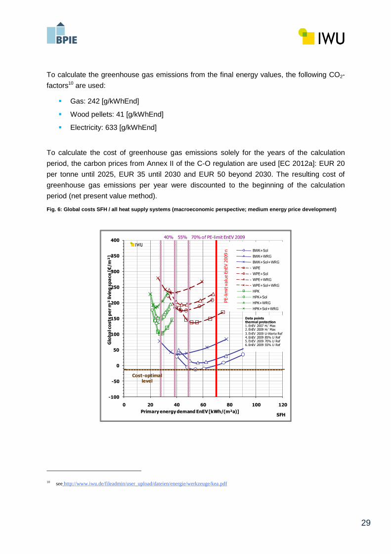
To calculate the greenhouse gas emissions from the final energy values, the following CO2-
factors10 are used:
Gas: 242 [g/kWhEnd]
Wood pellets: 41 [g/kWhEnd]
Electricity: 633 [g/kWhEnd]
To calculate the cost of greenhouse gas emissions solely for the years of the calculation
period, the carbon prices from Annex II of the C-O regulation are used [EC 2012a]: EUR 20
per tonne until 2025, EUR 35 until 2030 and EUR 50 beyond 2030. The resulting cost of
greenhouse gas emissions per year were discounted to the beginning of the calculation
period (net present value method).
Fig. 6: Global costs SFH / all heat supply systems (macroeconomic perspective; medium energy price development)
10 see http://www.iwu.de/fileadmin/user_upload/dateien/energie/werkzeuge/kea.pdf
Cost-optimal level
-100
-50
0
50
100
150
200
250
300
350
400
0 20 40 60 80 100 120
Glo
ba
l co
sts
pe
r m
² li
vin
g s
pa
ce
[€
/m
²]
BWK+Sol
BWK+WRG
BWK+Sol+WRG
WPE
WPE+Sol
WPE+WRG
WPE+Sol+WRG
HPK
HPK+Sol
HPK+WRG
HPK+Sol+WRG
40% 70% of PE-limit EnEV 2009 55%
SFH
Data points thermal protection1. EnEV 2007 HT' Max 2. EnEV 2009 HT' Max
3. EnEV 2009 U-Werte Ref4. EnEV 2009 85% U Ref5. EnEV 2009 70% U Ref6. EnEV 2009 55% U Ref
Primary energy demand EnEV [kWh/(m²a)]
PE-l
imit
valu
e E
nEV
2009 n

30
Fig. 7: Global costs MFH / all heat supply systems (macroeconomic perspective; medium energy price development)
The figures are showing that the cost-optimal levels do not change compared to the private
financial perspective (cost-optimal level 54 kWh/(m²a) for SFH and 53 kWh/(m²a) for MFH).
The considered cost of greenhouse gas emissions respect the assumed carbon prices from
Annex II of the C-O regulation but are too low to cause changes in cost-optimal levels.
Only the additional costs of advanced energy performance standards compared to EnEV 09
are decreasing from a macroeconomic perspective (see table below and tables 19 and 20 of
Annex 3).
Table 8: Increases of global costs towards nZEB compared to EnEV 09 (macroeconomic perspective)
Reference building “Cost-optimal level”
to EnEV 09
“Efficiency Building 55“
to EnEV 09
“Efficiency Building 40“
to EnEV 09
SFH -13 €/m² 43 €/m² 77 €/m²
MFH -8 €/m² 13 €/m² 27 €/m²
In the case of SFH the additional global costs of a “passive house” compared to EnEV 09 are
decreasing to 49 €/m² (6. data point of the curve “BWK+WRG”). The additional global costs
of a “passive house” in the case of MFH decrease to 72 €/m² (6. data point of the curve
“BWK+WRG”).
Cost-optimal level
-100
-50
0
50
100
150
200
250
300
350
0 20 40 60 80 100
Glo
ba
l co
sts
pe
r m
² li
vin
g s
pa
ce
[€
/m
²]
BWK+Sol
BWK+WRG
BWK+Sol+WRG
WPE
WPE+Sol
WPE+WRG
WPE+Sol+WRG
HPK
HPK+Sol
HPK+WRG
HPK+Sol+WRG
40% 70% of PE-limitEnEV 2009 55%
MFHPrimary energy demand EnEV [kWh/(m²a)]
Data points thermal protection1. EnEV 2007 HT' Max 2. EnEV 2009 HT' Max
3. EnEV 2009 U-Werte Ref4. EnEV 2009 85% U Ref5. EnEV 2009 70% U Ref6. EnEV 2009 55% U Ref
PE-l
imit
valu
e E
nEV
2009 n

31
3.3 Sensitivity analysis
A sensitivity analysis is performed on the discount rates and the energy performance
development exemplary from the private financial perspective. In the following, the results of
the sensitivity analysis regarding the cost-optimal levels and the additional costs of energy
performance standards towards nZEB are presented (for detailed figures see Annex 4). A
cost-optimal range is presented if the cost differences between two “cost-optimal levels” are
< 1 €/m². The most cost-effective variants towards nZEB do not change compared to the
basic scenario.
Discount rate
As alternative discount rate 1 % (real) is used. A lower discount rate means that all future
cost categories as well as the residual value are increasingly taken into consideration within
the NPV calculation compared to the basic scenario. In sum, for a discount rate of 1 % the
global costs are increasing but the cost-optimal levels are moving in the direction of lower
primary energy values, therefore the gap to current requirements of EnEV 09 is becoming
bigger and the additional costs of higher energy performance standards compared to EnEV
09 are decreasing (higher energy performance standards are becoming more profitable or
less non-profitable depending on the standard).
The results of the sensitivity analysis with a discount rate of 1 % are presented in tables 9
and 10.
Table 9: Results of sensitivity analysis discount rate SFH (medium energy price development)
DISCOUNT RATE 1 %
3 %
(BASIC SCENARIO)
Cost-optimal level [kWh/m²a] 48-54 54
Gap to EnEV 09 [kWh/m²a] (%) 22-16 (31%-23%) 16 (23%)
Additional costs CO to EnEV 09 [€/m²] -31 -12
Additional costs EB 55 to EnEV 09 [€/m²] +34 +58
Additional costs PH to EnEV 09 [€/m²] +23 +65
Additional costs EB 40 to EnEV 09 [€/m²] +59 +101
For the SFH the cost-optimal level is now described both of the 4. data point of the curve
“BWK+Sol” and the 5. data point of the curve “BWK+Sol” (cost-optimal range from 48-54
kWh/(m²a); the 4. data point (54 kWh/(m²a)) has minimal lower global costs < 1 €/m²)). The

32
additional costs of better energy performance standards (EB 55, EB 40, PH) are decreasing
compared to EnEV 09 (see in detail Annex 3 and 4: tables 17 and 25).
Table 10: Results of sensitivity analysis discount rate MFH (medium energy price development)
DISCOUNT RATE 1 %
3 %
(BASIC SCENARIO)
Cost-optimal level [kWh/m²a] 48 53
Gap to EnEV 09 [kWh/m²a] (%) 13 (21%) 8 (13%)
Additional costs CO to EnEV 09 [€/m²] -20 -8
Additional costs EB 55 to EnEV 09 [€/m²] +18 +23
Additional costs EB 40 to EnEV 09 [€/m²] +26 +41
Additional costs PH to EnEV 09 [€/m²] +120 +133
For the MFH the cost-optimal level moves from the 4. data point of the curve “BWK+Sol” to
the 5. data point of the curve “BWK+Sol” (cost-optimal level 48 kWh/(m²a)). The additional
costs of better energy performance standards (EB 55, EB 40, PH) are also decreasing
compared to EnEV 09 (see in detail Annex 3 and 4: tables 18 and 26).
Energy price development
Beside the basic scenario (2.8 %/a) two further scenarios of energy price development are
considered (see in detail Annex 4: tables 21, 22, 23 and 24).
A high energy price development (4.3 %/a) means that the net present value of future energy
costs is increasing compared to the basic scenario but the cost-optimal levels are moving in
the direction of lower primary energy values, the gap to current requirements of EnEV 09 is
becoming bigger and the additional costs of higher energy performance standards compared
to EnEV 09 are decreasing (higher energy performance standards are becoming more
profitable or less non-profitable depending on the standard).
A low energy price development (1.3 %/a) means that the net present value of future energy
costs is decreasing compared to the basic scenario but the cost-optimal levels are moving in
direction of higher primary energy values, the gap to current requirements of EnEV 09 is
becoming smaller and the additional costs of higher energy performance standards
compared to EnEV 09 are increasing (higher energy performance standards are becoming
less profitable or more non-profitable depending on the standard).
The results for SFH and MFH are shown in tables 11 and 12.

33
Table 11: Results of sensitivity analysis energy price development SFH (discount rate 3 %)
ENERGY PRICE DEVELOPMENT 1.3 % (REAL)
2.8 % (REAL)
(BASIC SCENARIO)
4.3 % (REAL)
Cost-optimal level [kWh/m²a] 60 54 54
Gap to EnEV 09 [kWh/m²a] (%) 10 (14%) 16 (23%) 16 (23%)
Additional costs CO to EnEV 09 [€/m²] -2 -12 -22
Additional costs EB 55 to EnEV 09 [€/m²] +81 +58 +37
Additional costs PH to EnEV 09 [€/m²] +84 +65 +47
Additional costs EB 40 to EnEV 09 [€/m²] +127 +101 +74
High energy price development SFH: The cost-optimal level is described still by the 4th data
point of the curve “BWK+Sol” (cost-optimal level 54 kWh/(m²a)). The additional costs of
better energy performance standards (EB 55, EB 40, PH) are decreasing compared to the
basic scenario.
Low energy price development SFH: The cost-optimal level moves to the 3th data point of the
curve “BWK+Sol” (cost-optimal level 60 kWh/(m²a)). The additional costs of better energy
performance standards (EB 55, EB 40, PH) are increasing compared to the basic scenario.
Table 12: Results of sensitivity analysis energy price development MFH (discount rate 3 %)
ENERGY PRICE DEVELOPMENT 1.3 % (REAL)
2.8 % (REAL)
(BASIC SCENARIO)
4.3 % (REAL)
Cost-optimal level [kWh/m²a] 53 53 48-53
Gap to EnEV 09 [kWh/m²a] (%) 8 (13%) 8 (13%) 13-8 (21%-13%)
Additional costs CO to EnEV 09 [€/m²] -4 -8 -12
Additional costs EB 55 to EnEV 09 [€/m²] +22 +23 +24
Additional costs EB 40 to EnEV 09 [€/m²] +42 +41 +39
Additional costs PH to EnEV 09 [€/m²] +147 +133 +114
High energy price development MFH: The cost-optimal level is described now both of the 4th
data point of the curve “BWK+Sol” and the 5th data point of the curve “BWK+Sol” (cost-
optimal range from 48-53 kWh/(m²a); the 4th data point has minimal lower global costs < 1
€/m²)). The additional costs of better energy performance standards stay nearly constant (EB
55) or are decreasing (EB 40, PH) compared to the basic scenario.
Low energy price development MFH: The cost-optimal level is described still by the 4th data
point of the curve “BWK+Sol” (cost-optimal level 53 kWh/(m²a)). The additional costs of

34
better energy performance standards stay nearly constant (EB 55) or are increasing (EB 40,
PH) compared to the basic scenario.
Due to lower actual energy prices for wood pellets and relatively high energy use for heating
and hot water, the effect of a low (high) energy price development on the additional costs is
less obvious for the variants with wood pellet boiler in the MFH (EB 55 and 40). In the case
of EB 55 the net present value of energy costs is even decreasing (increasing) more than for
the variant EnEV 09 (with gas condensing boiler and solar heating system).
Discount rate 1 % (real) and high energy price development
An additionally variation of input parameters was carried out exemplary for the SFH
reference building for a high energy price development scenario and a low discount rate of 1
%. The results are shown in figure 8 (see also table 27 in Annex 4). The changes are
obvious especially for the heat supply systems with condensing boiler. The cost-optimal
primary energy demand moves to approx. 48 kWh/m²/a and the additional costs from EnEV
09 to nZEB level are decreasing e.g. for efficiency building 40 from 101 €/m² to 19 €/m² (see
table 13).
Compared to the current minimum energy performance requirements of EnEV 2009
(intersection of the red vertical line with the curve “BWK+Sol”) the energy performance
standards efficiency building 55 (5. data point of the curve “BWK+Sol+WRG) and passive
house (6th data point of the curve “BWK+WRG) could now be realised with nearly the same
or in the case of PH even with lower global costs.

35
Fig. 8: Global costs SFH / all heat supply systems (high energy price development/discount rate 1 %)
Table 13: Results of sensitivity analysis SFH (high energy price development; low discount rate)
ENERGY PRICE DEVELOPMENT / DISCOUNT RATE 4.3 % (REAL) / 1 % 2.8 % (REAL) / 3 %
(BASIC SCENARIO)
Cost-optimal level [kWh/m²a] 48 54
Gap to EnEV 09 [kWh/m²a] (%) 22 (31%) 16 (23%)
Additional costs CO to EnEV 09 [€/m²] -52 -12
Additional costs PH to EnEV 09 [€/m²] -3 +65
Additional costs EB 55 to EnEV 09 [€/m²] +2 +58
Additional costs EB 40 to EnEV 09 [€/m²] +19 +101
Disposal costs
Furthermore disposal costs are exemplarily considered for one reference building and
thermal protection measures. The disposal costs at the end of the lifetime (50 years) are
assumed to an overall percentage (30 %) of the initial investment costs. Discounted to the
end of the calculation period the disposal costs are reducing the residual value of the
insulation measures by about 17 %. As a result, the global costs are increasing marginal and
Cost-optimal
level-100
-50
0
50
100
150
200
250
300
350
400
0 20 40 60 80 100 120
Glo
ba
l co
sts
pe
r m
² liv
ing
sp
ace
[€
/m
²]
BWK+Sol
BWK+WRG
BWK+Sol+WRG
WPE
WPE+Sol
WPE+WRG
WPE+Sol+WRG
HPK
HPK+Sol
HPK+WRG
HPK+Sol+WRG
40% 70% of PE-limit EnEV 2009 55%
SFH
D at a po int s
t hermal p ro t ect ion
1. EnEV 2007 HT ' M ax
2. EnEV 2009 HT ' M ax
3. EnEV 2009 U-Werte Ref
4. EnEV 2009 85% U Ref
5. EnEV 2009 70% U Ref
6. EnEV 2009 55% U Ref
Primary energy demand EnEV [kWh/(m²a)]
PE-l
imit
valu
e E
nEV
2009 n

36
the cost-optimum moves slight to the right. Due to discounting the influence of future disposal
costs on the cost-optimal level remains marginal.

37
References
[BMVBS 2010] BMVBS (Hrsg.): Externe Kosten im Hochbau, BMVBS-Online-
Publikation, Nr. 17/2010
[EC 2010] EU energy trends to 2030 – update 2009; European
Commission; 2010
[EC 2012a] Commission Regulation (EU) No 244/2012 of 16 January 2012;
supplementing Directive 2010/31/EU of the European
Parliament and of the Council on the energy performance of
buildings (recast) by establishing a comparative methodology
framework for cost optimal levels of minimum energy
performance requirements for buildings and building elements
[EC 2012b] Guidelines accompanying the document Commission
Delegated Regulation No 244/2012 of 16 January 2012;
supplementing Directive 2010/31/EU of the European
Parliament and of the Council on the energy performance of
buildings (recast) by establishing a comparative methodology
framework for cost optimal levels of minimum energy
performance requirements for buildings and building elements
[Hinz 2010] Hinz, E.: Untersuchung zur weiteren Verschärfung der
energetischen Anforderungen an Wohngebäude mit der EnEV
2012. Teil 1 - Kosten energierelevanter Bau- und Anlagenteile
in der energetischen Modernisierung von Altbauten; im Auftrag
des BBSR; IWU; Darmstadt 2010
[IWU 2012] Diefenbach, N., Enseling, A., Hinz, E., Loga, T.:
Evaluierung und Fortentwicklung der EnEV 2009: Untersuchung
zu ökonomischen Rahmenbedingungen im Wohnungsbau; im
Auftrag des BBSR; IWU / BBSR 2012

38
[ZUB 2010] Klauß, Swen; Maas, Anton: Entwicklung einer Datenbank mit
Modellgebäuden für energiebezogene Untersuchungen,
insbesondere der Wirtschaftlichkeit; Studie durchgeführt im
Auftrag des BMVBS sowie des BBSR; Zentrum für
Umweltbewusstes Bauen e.V., Kassel 2010

39
Annex 1: Initial investment costs
The following table shows the used parameters of the cost functions (additional costs) for
thermal protection measures on building elements.
Table 14: Parameters of the cost functions (additional costs) for thermal protection measures on building elements
arithmetic averages used approach (rounded)
specific costs
thermal resistance
specific costs
insulation
specific costs thermal
resistance
specific costs
insulation
€/(m²K) €/cm/m² €/(m²K/W) €/cm/m²
Flat roof 3,96 1,13 1,1 Steep roof 9,54 2,72 2,7 Outer wall 5,85 1,67 1,7 Cellar ceiling 5,88 1,68 1,7 Window 299 300 Roof window 786 800 External door 1057 1100
Based on the shown parameters, the following dependences between initial investment costs
and U-values of building components become obvious. Important are only the differences
between two thermal protection standards – the zero-point is randomised.
Fig. 9: Initial investment costs as a function of u-values for building components
0
20
40
60
80
100
120
0,0 0,1 0,2 0,3 0,4 0,5
U-Wert [W/(m²K]
Inve
stit
ion
sko
sten
pro
m²
Bau
teil
[€/m
²] Steildach
Flachdach
Außenwand
Kellerdecke
0
50
100
150
200
250
300
350
0,6 0,8 1,0 1,2 1,4 1,6
U-Wert [W/(m²K]
Inve
stit
ion
sko
sten
pro
m²
Bau
teil
[€/m
²] Fenster

40
The following table shows the used difference costs for energy saving installations.
Table 15: Difference costs for technical installations
SFH MFH
Heat generator: cost difference compared to system with gas condensing boiler
Woodpellet boiler + 80 €/m² + 31 €/m²
Electrical heat pump (heat source: ground) + 121 €/m² + 60 €/m²
Heat distribution and emission: cost difference compared to system with standard radiators
Under floor heating + 20 €/m² + 25 €/m²
Additional costs of supplemental systems
Thermal solar DHW system
+ 35 €/m² + 35 €/m²
Exhaust ventilation system, including supply air valves + 20 €/m² + 37 €/m²
Ventilation system with heat recovery (thermal efficiency 80%) + 64 €/m² + 110 €/m²
Costs savings due to reduced heating power (best standard compared to poorest standard)
Heat generators
Gas condensing boiler - € - €
Woodpellets boiler - € - €
Electrical heat pump (heat source: ground) -5 € -10 €
Heat emission system
Standard radiators -4 € -4 €
Under floor heating -6 € -6 €

41
Annex 2: Reporting table for energy performance relevant data
Table 16: Reporting table for energy performance relevant data (Table 3 of [EC 2012b])
Quantity Unit
Building Model building SFH semi-detached
MFH semi-detached
Variant requirements of EnEV 2009 and EEWärmeG; assuming condensing boilers + thermal solar systems
Calculation Method and tool(s) EnEV 2009 / DIN V 4108-6 + DIN V 4701-10 calculation tool: EnEV-XL 4.0
Primary energy conversion factors
natural gas: 1.1 electricity: 2.6 wood pellets: 0.2
Climate condition
Location reference climate Germany (synthetical climate)
Heating degree-days according to DIN V 4108-6 (base temperature 10°C): (10 °C - 3.3°C) · 185 d/a = 1240 Kd/a according to TABULA (base temperature 12°C, see www.building-typology.eu): (12 °C - 4.4°C) · 222 d/a = 1687 Kd/a
Source of climatic dataset reference climate Germany, according to DIN V 4108-6 Part D
Reference area
Living space according to national housing regulations
139.0 473.0 m²
Reference area according to national asset rating method
187.5 591.4 m²
Building geometry
Length x Width x Height external dimensions: 7.5 x 11.4 x 9.7 (internal dimensions cannot be determined due to lack of plans)
external dimensions: 11.0 x 14.0 x 12.0 (internal dimensions cannot be determined due to lack of plans)
m x m x m
Number of floors 1 complete storey + attic storey
4 complete storeys
Surface to volume ratio 0.59 (based on external
dimensions)
0.42 (based on external
dimensions)
m²/m³
Ratio of window area over total building envelope
South 3.3% 0.0%
East 2.5% 7.0%
North 1.7% 0.0%
West 0.0% 8.5%
Orientation 0° 0°
Internal gains Building utilisation residential residential W/m²
Average thermal gain sum of all sources: 5
sum of all sources: 5
W/m²

42
Building elements
Average U-value of walls 0.33 0.29 W/(m²K)
Average U-value of roof 0.31 0.26 W/(m²K)
Average U-value of basement 0.48 0.43 W/(m²K)
Average U-value of windows 1.30 1.30 W/(m²K)
Thermal bridges
additional losses related to the thermal envelope area
0.02 (based on external
dimensions)
0.02 (based on external
dimensions)
W/(m²K)
Infiltration rate (air changes per hour)
blower door: 50 Pa
3.0 (requirement for buildings without ventilation system)
3.0 (requirement for buildings without ventilation system)
1/h
Building systems
Efficiencies of heating systems (related to net calorific value)
generation 104.2% 102.2%
distribution 2.1% 2.4%
emission + control
1.4% 2.0%
Efficiencies of DHW systems (related to net calorific value)
generation 89.1% 91.2%
storage 12.6% 11.0%
distribution 23.1% 40.3%
Building energy need / use (related to living space)
Energy need heating 78 56 kWh/(m²a)
DHW 17 16 kWh/(m²a)
Energy use for auxiliary systems
5 3 kWh/(m²a)
Thermal energy from RES (thermal solar collector)
16 14 kWh/(m²a)
Delivered energy for heating and DHW
electricity 0 0 kWh/(m²a)
fossil fuel (natural gas)
74 43 kWh/(m²a)
biomass (wood pellets)
0 0 kWh/(m²a)
Environ-mental assessment
Primary energy 94 59 kWh/(m²a)
43
Annex 3: Global cost calculation – output data
In the following, the global costs calculation from the private financial and the
macroeconomic perspective is documented with regard to table 6 of Annex III of the C-O
regulation. The documented initial investment costs for thermal protection and technical
installations are calculated as difference costs referring to a given basis (see Annex 1) and
are including replacement costs for technical installations. For the sake of clarity, only the
most important variants are presented for both reference buildings. The most cost-effective
variants towards nZEB levels are highlighted in grey. The additional costs of these standards
compared to EnEV 09 are resulting as differences from the global cost calculated for the
nZEB variants and the global cost calculated for EnEV 09.

44
Table 17: Output data and global cost calculation SFH (selected variants; private financial perspective)
Calculation period:
30 years
0,67
13,12
0,64
12,63
1,51
29,68
0,80
15,69
1,50
29,41
1,53
30,07
1,52
29,80
2,40
47,06
2,97
58,25
3,12
61,18
3,82
74,90
EB 55
(5/HPK)212,86 181,81 14,37 3%
Insulation:
50
Windows:
30
Installations:
15
410,36
EB 40
(6/HPK)288,81 160,82 27,09 3%
Insulation:
50
Windows:
30
Installations:
15
452,35
PH
(6/HPK+WRG)360,97 130,83 27,09 3%
Insulation:
50
Windows:
30
Installations:
15
511,77
EB 55
(5/WPE+Sol)330,69 122,64 14,37 3%
Insulation:
50
Windows:
30
Installations:
15
497,21
PH
(6/WPE+WRG)420,01 110,16 27,09 3%
Insulation:
50
Windows:
30
Installations:
15
564,26
EB 40
(6/WPE+Sol+WRG)477,41 87,18 27,09 3%
Insulation:
50
Windows:
30
Installations:
15
612,41
Energy costs by fuel
medium energy
price scenario
[€/m²] (NPV)
Residual
value
[€/m²]
(NPV)
336,29
EB 55
(5/BWK+Sol+WRG)211,22
372,29EB 40
(6/BWK+Sol+WRG)287,17 82,79 27,09 3%
Insulation:
50
Windows:
30
Installations:
15
PH
(6/BWK+WRG)229,77 117,92 27,09 3%
Insulation:
50
Windows:
30
Installations:
15
Insulation:
50
Windows:
30
Installations:
15
259,88
EnEV 09 (BWK+Sol)
75,65
103,55 14,37 3%
Insulation:
50
Windows:
30
Installations:
15
330,07
186,35 3,43 3%
Insulation:
50
Windows:
30
Installations:
15
271,69
Cost optimum
(4/BWK+Sol) 109,59 147,02 9,36 3%
Estimated
economic
lifetime
[a]
Global
cost
calculated
[€/m²]maintenance
cost
[€/m²a] /
[€/m²] (NPV)
Variant Initial
investment cost
(including NPV
replacement
cost)
[€/m²]
Annual
running cost
Discount
rate
[%]

45
Table 18: Output data and global cost calculation MFH (selected variants; private financial perspective)
Calculation period:
30 years
0,66
12,97
0,00
12,64
2,09
41,02
2,08
40,78
1,24
24,31
0,55
10,82
0,54
10,59
2,00
39,22
1,62
31,76
2,38
46,67
3,08
60,39
462,94EB 40
(6/WPE+Sol+WRG)342,57 74,83 14,85 3%
Insulation:
50
Windows: 30
Installations:
15
332,80
PH
(6/WPE+WRG)285,17 94,72 14,85 3%
Insulation:
50
Windows: 30
Installations:
15
411,71
EB 55
(6/WPE+Sol)222,85
254,01 115,11 14,85 3%
93,04 14,85 3%
Insulation:
50
Windows: 30
Installations:
15
Insulation:
50
Windows: 30
Installations:
15
393,48
EB 40
(6/HPK)134,29 142,21 14,85 3%
Insulation:
50
Windows: 30
Installations:
15
272,24
PH
(6/HPK+WRG)
318,12
EB 55
(5/HPK)97,94 154,74 8,69 3%
Insulation:
50
Windows: 30
Installations:
15
254,80
EB 40
(6/HPK+Sol)191,69
260,57 77,71 14,85 3%
116,97 14,85 3%
Insulation:
50
Windows: 30
Installations:
15
Insulation:
50
Windows: 30
Installations:
15
364,21
EB 55
(5/BWK+Sol+WRG)224,22 90,50 8,69 3%
Insulation:
50
Windows: 30
Installations:
15
347,04
PH
(6/BWK+WRG)
3%
Insulation:
50
Windows: 30
Installations:
15
231,69
Cost optimum
(4/BWK+Sol) 84,59 132,08 5,23 3%
Insulation:
50
Windows: 30
Installations:
15
224,08
EnEV 09
(BWK+Sol)70,95 150,53 2,76
Discount
rate
[%]
Estimated
economic
lifetime
[a]
Global
cost
calculated
[€/m²]maintenance
cost
[€/m²a] / [€/m²]
(NPV)
Energy costs by fuel
medium energy
price scenario
[€/m²] (NPV)
Annual
running cost
Residual
value
[€/m²]
(NPV)
Variant Initial
investment cost
(including NPV
replacement
cost)
[€/m²]

46
Table 19: Output data and global cost calculation SFH (selected variants; macroeconomic perspective)
Calculation
period:
30 years
0,56
11,02
0,54
10,62
1,27
24,94
0,67
13,18
1,26
24,72
1,29
25,27
1,28
25,05
2,02
39,55
2,50
48,95
2,62
51,41
3,21
62,94
Variant Initial
investment
cost
(including
NPV
replacement
cost)
[€/m²]
Annual
running cost
Residual
value
[€/m²]
(NPV)
Discount
rate
[%]
Estimated
economic
lifetime
[a]
maintenance
cost
[€/m²a] /
[€/m²] (NPV)
Energy costs
by fuel
medium
energy price
scenario
[€/m²] (NPV)
Global
cost
calculated
[€/m²]
EnEV 09
(BWK+Sol)63,57 156,60 2,88 3%
Insulation:
50
Windows:
30
Installations:
15
241,29
Cost optimum
(4/BWK+Sol) 92,10 123,54 7,87 3%
Insulation:
50
Windows:
30
Installations:
15
228,48
EB 55
(5/BWK+Sol+WRG)177,49 87,01 12,08 3%
Insulation:
50
Windows:
30
Installations:
15
284,08
PH
(6/BWK+WRG)193,08 99,10 22,76 3%
Insulation:
50
Windows:
30
Installations:
15
290,43
EB 40
(6/BWK+Sol+WRG)241,32 69,58 22,76 3%
Insulation:
50
Windows:
30
Installations:
15
318,03
EB 55
(5/HPK)178,87 152,78 12,08 3%
Insulation:
50
Windows:
30
Installations:
15
349,59
EB 40
(6/HPK)242,70 135,14 22,76 3%
Insulation:
50
Windows:
30
Installations:
15
384,51
PH
(6/HPK+WRG)303,34 109,94 22,76 3%
Insulation:
50
Windows:
30
Installations:
15
434,28
EB 55
(5/WPE+Sol)277,89 103,06 12,08 3%
Insulation:
50
Windows:
30
Installations:
15
425,69
PH
(6/WPE+WRG)352,95 92,58 22,76 3%
Insulation:
50
Windows:
30
Installations:
15
481,04
EB 40
(6/WPE+Sol+WRG)401,18 73,26 22,76 3%
Insulation:
50
Windows:
30
Installations:
15
519,85
Cost of
green
house gas
emissions
[€/m²]
12,97
10,09
6,71
7,83
5,19
4,74
4,38
4,22
7,87
6,87
5,22

47
Table 20: Output data and global cost calculation MFH (selected variants; macroeconomic perspective)
Calculation
period:
30 years
0,56
10,90
0,54
10,62
1,76
34,47
1,16
22,74
1,04
20,43
0,46
9,09
0,45
8,90
1,68
32,95
1,36
26,69
2,00
39,22
2,59
50,75
Residual
value
[€/m²]
(NPV)
Discount
rate
[%]
Estimated
economic
lifetime
[a]
Global
cost
calculated
[€/m²]
maintenance
cost
[€/m²a] /
[€/m²] (NPV)
Energy costs
by fuel
medium
energy price
scenario
[€/m²] (NPV)
Variant Initial
investment
cost
(including
NPV
replacement
cost)
[€/m²]
Annual
running cost
EnEV 09
(BWK+Sol)59,62 126,50 2,32 3%
Insulation:
50
Windows: 30
Installations:
15
205,25
Cost optimum
(4/BWK+Sol) 71,08 110,99 4,40 3%
Insulation:
50
Windows: 30
Installations:
15
197,51
EB 55
(5/BWK+Sol+WRG)188,42 76,05 7,31 3%
Insulation:
50
Windows: 30
Installations:
15
297,61
PH
(6/BWK+WRG)170,73 89,47 12,48 3%
Insulation:
50
Windows: 30
Installations:
15
277,63
EB 40
(6/HPK+Sol)161,08 98,30 12,48 3%
Insulation:
50
Windows: 30
Installations:
15
270,68
EB 55
(5/HPK)82,30 130,03 7,31 3%
Insulation:
50
Windows: 30
Installations:
15
218,053,94
EB 40
(6/HPK)112,85 119,51 12,48 3%3,72
Insulation:
50
Windows: 30
Installations:
15
232,49
PH
(6/HPK+WRG)213,45 96,73 12,48 3%
Insulation:
50
Windows: 30
Installations:
15
334,243,58
EB 55
(6/WPE+Sol)187,27 78,19 12,48 3%5,99
Insulation:
50
Windows: 30
Installations:
15
285,65
PH
(6/WPE+WRG)239,64 79,60 12,48 3%
Insulation:
50
Windows: 30
Installations:
15
351,935,96
EB 40
(6/WPE+Sol+WRG)287,87 62,89 12,48 3%4,56
Insulation:
50
Windows: 30
Installations:
15
393,58
Cost of
green
house gas
emissions
[€/m²]
10,55
9,20
5,97
7,17
3,35

48
Annex 4: Sensitivity analysis – output data
Energy price development
Fig. 10: Global costs SFH / MFH all heat supply systems (high energy price development)
Fig. 11: Global costs SFH / MFH all heat supply systems (low energy price development)
Cost-optimal
level
-100
-50
0
50
100
150
200
250
300
350
400
0 20 40 60 80 100 120
Glo
ba
l co
sts
pe
r m
² liv
ing
sp
ace
[€
/m
²]
BWK+Sol
BWK+WRG
BWK+Sol+WRG
WPE
WPE+Sol
WPE+WRG
WPE+Sol+WRG
HPK
HPK+Sol
HPK+WRG
HPK+Sol+WRG
40% 70% of PE-limit EnEV 2009 55%
SFH
D at a po int s
t hermal p ro t ect ion
1. EnEV 2007 HT ' M ax
2. EnEV 2009 HT ' M ax
3. EnEV 2009 U-Werte Ref
4. EnEV 2009 85% U Ref
5. EnEV 2009 70% U Ref
6. EnEV 2009 55% U Ref
Primary energy demand EnEV [kWh/(m²a)]
PE-l
imit
valu
e E
nEV
2009 n
Cost-optimal
level
-100
-50
0
50
100
150
200
250
300
350
0 20 40 60 80 100
Glo
ba
l co
sts
pe
r m
² liv
ing
sp
ace
[€
/m
²]
BWK+Sol
BWK+WRG
BWK+Sol+WRG
WPE
WPE+Sol
WPE+WRG
WPE+Sol+WRG
HPK
HPK+Sol
HPK+WRG
HPK+Sol+WRG
40% 70% of PE-limitEnEV 2009 55%
MFHPrimary energy demand EnEV [kWh/(m²a)]
D at a po int s
t hermal p ro t ect ion
1. EnEV 2007 HT ' M ax
2. EnEV 2009 HT ' M ax
3. EnEV 2009 U-Werte Ref
4. EnEV 2009 85% U Ref
5. EnEV 2009 70% U Ref
6. EnEV 2009 55% U Ref
PE-l
imit
valu
e E
nEV
2009 n
Cost-optimal
level
-100
-50
0
50
100
150
200
250
300
350
400
0 20 40 60 80 100 120
Glo
ba
l co
sts
pe
r m
² liv
ing
sp
ace
[€
/m
²]
BWK+Sol
BWK+WRG
BWK+Sol+WRG
WPE
WPE+Sol
WPE+WRG
WPE+Sol+WRG
HPK
HPK+Sol
HPK+WRG
HPK+Sol+WRG
40% 70% of PE-limit EnEV 2009 55%
SFH
D at a po int s
t hermal p ro t ect ion
1. EnEV 2007 HT ' M ax
2. EnEV 2009 HT ' M ax
3. EnEV 2009 U-Werte Ref
4. EnEV 2009 85% U Ref
5. EnEV 2009 70% U Ref
6. EnEV 2009 55% U Ref
Primary energy demand EnEV [kWh/(m²a)]
PE-l
imit
valu
e E
nEV
2009 n
Cost-optimal
level
-100
-50
0
50
100
150
200
250
300
350
0 20 40 60 80 100
Glo
ba
l co
sts
pe
r m
² liv
ing
sp
ace
[€
/m
²]
BWK+Sol
BWK+WRG
BWK+Sol+WRG
WPE
WPE+Sol
WPE+WRG
WPE+Sol+WRG
HPK
HPK+Sol
HPK+WRG
HPK+Sol+WRG
40% 70% of PE-limitEnEV 2009 55%
MFHPrimary energy demand EnEV [kWh/(m²a)]
D at a po int s
t hermal p ro t ect ion
1. EnEV 2007 HT ' M ax
2. EnEV 2009 HT ' M ax
3. EnEV 2009 U-Werte Ref
4. EnEV 2009 85% U Ref
5. EnEV 2009 70% U Ref
6. EnEV 2009 55% U Ref
PE-l
imit
valu
e E
nEV
2009 n

49
Table 21: Output data and global cost calculation SFH (selected variants; private financial perspective; high energy
price development)
Calculation period:
30 years
0,67
13,12
0,64
12,63
1,51
29,68
0,80
15,69
1,50
29,41
1,53
30,07
1,52
29,80
2,40
47,06
2,97
58,25
3,12
61,18
3,82
74,90
Variant Initial
investment cost
(including NPV
replacement
cost)
[€/m²]
Annual
running cost
3,43 3%
Insulation:
50
Windows: 30
Installations:
15
maintenance
cost
[€/m²a] /
[€/m²] (NPV)
319,22
Cost optimum
(4/BWK+Sol) 109,59 184,51 9,36 3%
Insulation:
50
Windows: 30
Installations:
15
297,38
EnEV 09
(BWK+Sol)75,65
366,37
EB 55
(5/BWK+Sol+WRG)129,96 14,37 3%
Insulation:
50
Windows: 30
Installations:
15
PH
(6/BWK+WRG)229,77 148,00 27,09
EB 40
(6/BWK+Sol+WRG)287,17 103,91 27,09
211,22
393,403%
Insulation:
50
Windows: 30
Installations:
15
356,48
233,88
3%
Insulation:
50
Windows: 30
Installations:
15
Estimated
economic
lifetime
[a]
Global
cost
calculated
[€/m²]Energy costs by fuel
medium energy
price scenario
[€/m²] (NPV)
Residual
value
[€/m²]
(NPV)
Discount
rate
[%]
592,36
EB 40
(6/WPE+Sol+WRG)477,41 109,42 27,09 3%
Insulation:
50
Windows: 30
Installations:
15
634,64
PH
(6/WPE+WRG)420,01 138,26 27,09 3%
Insulation:
50
Windows: 30
Installations:
15
545,14
EB 55
(5/WPE+Sol)330,69 153,91 14,37 3%
Insulation:
50
Windows: 30
Installations:
15
528,48
PH
(6/HPK+WRG)360,97 164,20 27,09 3%
Insulation:
50
Windows: 30
Installations:
15
456,73
EB 40
(6/HPK)288,81 201,84 27,09 3%
Insulation:
50
Windows: 30
Installations:
15
493,36
EB 55
(5/HPK)212,86 228,17 14,37 3%
Insulation:
50
Windows: 30
Installations:
15

50
Table 22: Output data and global cost calculation MFH (selected variants; private financial perspective; high energy
price development)
Calculation period:
30 years
0,66
12,97
0,00
12,64
2,09
41,02
2,08
40,78
1,24
24,31
0,55
10,82
0,54
10,59
2,00
39,22
1,62
31,76
2,38
46,67
3,08
60,39
Variant Initial
investment cost
(including NPV
replacement
cost)
[€/m²]
Discount
rate
[%]
Estimated
economic
lifetime
[a]
Global
cost
calculated
[€/m²]maintenance
cost
[€/m²a] / [€/m²]
(NPV)
Energy costs by fuel
medium energy
price scenario
[€/m²] (NPV)
Annual
running cost
Residual
value
[€/m²]
(NPV)
EnEV 09
(BWK+Sol)70,95 188,92 2,76 3%
Insulation:
50
Windows: 30
Installations:
15
270,08
Cost optimum
(4/BWK+Sol) 84,59 165,77 5,23 3%
Insulation:
50
Windows: 30
Installations:
15
257,76
Insulation:
50
Windows: 30
Installations:
15
384,03
EB 55
(5/BWK+Sol+WRG)224,22 113,59 8,69 3%
Insulation:
50
Windows: 30
Installations:
15
370,12
PH
(6/BWK+WRG)
146,81 14,85 3%
Insulation:
50
Windows: 30
Installations:
15
260,57 97,53 14,85 3%
347,96
EB 55
(5/HPK)97,94 194,20 8,69 3%
Insulation:
50
Windows: 30
Installations:
15
294,26
EB 40
(6/HPK+Sol)191,69
Insulation:
50
Windows: 30
Installations:
15
422,84
EB 40
(6/HPK)134,29 178,48 14,85 3%
Insulation:
50
Windows: 30
Installations:
15
308,51
PH
(6/HPK+WRG)
116,77 14,85 3%
Insulation:
50
Windows: 30
Installations:
15
254,01 144,46 14,85 3%
356,53
PH
(6/WPE+WRG)285,17 118,88 14,85 3%
Insulation:
50
Windows: 30
Installations:
15
435,86
EB 55
(6/WPE+Sol)222,85
482,03EB 40
(6/WPE+Sol+WRG)342,57 93,92 14,85 3%
Insulation:
50
Windows: 30
Installations:
15
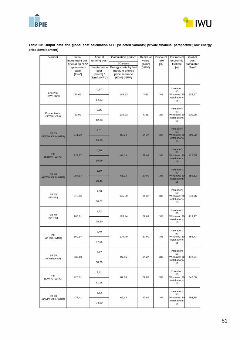
51
Table 23: Output data and global cost calculation SFH (selected variants; private financial perspective; low energy
price development)
Calculation period:
30 years
0,67
13,12
0,65
12,83
1,51
29,68
0,80
15,69
1,50
29,41
1,53
30,07
1,52
29,80
2,40
47,06
2,97
58,25
3,12
61,18
3,82
74,90
145,20 14,37 3%
Insulation:
50
Windows: 30
Installations:
15
373,76
EB 40
(6/HPK)288,81 128,44 27,09 3%
Insulation:
50
Windows: 30
Installations:
15
419,97
EB 55
(5/HPK)212,86
104,49 27,09 3%
Insulation:
50
Windows: 30
Installations:
15
485,43
EB 55
(5/WPE+Sol)330,69 97,95 14,37 3%
Insulation:
50
Windows: 30
Installations:
15
472,51
PH
(6/HPK+WRG)360,97
87,98 27,09 3%
Insulation:
50
Windows: 30
Installations:
15
542,08
EB 40
(6/WPE+Sol+WRG)477,41 69,63 27,09 3%
Insulation:
50
Windows: 30
Installations:
15
594,85
PH
(6/WPE+WRG)420,01
Estimated
economic
lifetime
[a]
Global
cost
calculated
[€/m²]Energy costs by fuel
medium energy
price scenario
[€/m²] (NPV)
Residual
value
[€/m²]
(NPV)
211,22
355,62EB 40
(6/BWK+Sol+WRG)287,17 66,12 27,09 3%
Insulation:
50
Windows: 30
Installations:
15
309,22
148,83
PH
(6/BWK+WRG)229,77 94,18 27,09 3%
Insulation:
50
Windows: 30
Installations:
15
312,55
EB 55
(5/BWK+Sol+WRG)82,70 14,37 3%
Insulation:
50
Windows: 30
Installations:
15
228,67
Cost optimum
(3/BWK+Sol) 91,92 130,23 6,31 3%
Insulation:
50
Windows: 30
Installations:
15
230,28
EnEV 09
(BWK+Sol)75,65
Discount
rate
[%]
3,43 3%
Insulation:
50
Windows: 30
Installations:
15
maintenance
cost
[€/m²a] /
[€/m²] (NPV)
Variant Initial
investment cost
(including NPV
replacement
cost)
[€/m²]
Annual
running cost

52
Table 24: Output data and global cost calculation MFH (selected variants; private financial perspective; low energy
price development)
Calculation period:
30 years
0,66
12,97
0,00
12,64
2,09
41,02
2,08
40,78
1,24
24,31
0,55
10,82
0,54
10,59
2,00
39,22
1,62
31,76
2,38
46,67
3,08
60,39
447,88EB 40
(6/WPE+Sol+WRG)342,57 59,77 14,85 3%
Insulation:
50
Windows: 30
Installations:
15
314,07
PH
(6/WPE+WRG)285,17 75,65 14,85 3%
Insulation:
50
Windows: 30
Installations:
15
392,63
EB 55
(6/WPE+Sol)222,85
254,01 91,93 14,85 3%
74,31 14,85 3%
Insulation:
50
Windows: 30
Installations:
15
Insulation:
50
Windows: 30
Installations:
15
370,30
EB 40
(6/HPK)134,29 113,58 14,85 3%
Insulation:
50
Windows: 30
Installations:
15
243,60
PH
(6/HPK+WRG)
294,57
EB 55
(5/HPK)97,94 123,58 8,69 3%
Insulation:
50
Windows: 30
Installations:
15
223,64
EB 40
(6/HPK+Sol)191,69
260,57 62,06 14,85 3%
93,42 14,85 3%
Insulation:
50
Windows: 30
Installations:
15
Insulation:
50
Windows: 30
Installations:
15
348,56
EB 55
(5/BWK+Sol+WRG)224,22 72,28 8,69 3%
Insulation:
50
Windows: 30
Installations:
15
328,82
PH
(6/BWK+WRG)
3%
Insulation:
50
Windows: 30
Installations:
15
201,38
Cost optimum
(4/BWK+Sol) 84,59 105,49 5,23 3%
Insulation:
50
Windows: 30
Installations:
15
197,49
EnEV 09
(BWK+Sol)70,95 120,22 2,76
Discount
rate
[%]
Estimated
economic
lifetime
[a]
Global
cost
calculated
[€/m²]maintenance
cost
[€/m²a] / [€/m²]
(NPV)
Energy costs by fuel
medium energy
price scenario
[€/m²] (NPV)
Annual
running cost
Residual
value
[€/m²]
(NPV)
Variant Initial
investment cost
(including NPV
replacement
cost)
[€/m²]

53
Discount rate
Fig. 12: Global costs SFH / MFH all heat supply systems (discount rate 1 %)
Cost-optimal
level
-100
-50
0
50
100
150
200
250
300
350
400
0 20 40 60 80 100 120
Glo
ba
l co
sts
pe
r m
² liv
ing
sp
ace
[€
/m
²]
BWK+Sol
BWK+WRG
BWK+Sol+WRG
WPE
WPE+Sol
WPE+WRG
WPE+Sol+WRG
HPK
HPK+Sol
HPK+WRG
HPK+Sol+WRG
40% 70% of PE-limit EnEV 2009 55%
SFH
D at a po int s
t hermal p ro t ect ion
1. EnEV 2007 HT ' M ax
2. EnEV 2009 HT ' M ax
3. EnEV 2009 U-Werte Ref
4. EnEV 2009 85% U Ref
5. EnEV 2009 70% U Ref
6. EnEV 2009 55% U Ref
Primary energy demand EnEV [kWh/(m²a)]
PE-l
imit
valu
e E
nEV
2009 n
Cost-optimal
level
-100
-50
0
50
100
150
200
250
300
350
0 20 40 60 80 100
Glo
ba
l co
sts
pe
r m
² liv
ing
sp
ace
[€
/m
²]
BWK+Sol
BWK+WRG
BWK+Sol+WRG
WPE
WPE+Sol
WPE+WRG
WPE+Sol+WRG
HPK
HPK+Sol
HPK+WRG
HPK+Sol+WRG
40% 70% of PE-limitEnEV 2009 55%
MFHPrimary energy demand EnEV [kWh/(m²a)]
D at a po int s
t hermal p ro t ect ion
1. EnEV 2007 HT ' M ax
2. EnEV 2009 HT ' M ax
3. EnEV 2009 U-Werte Ref
4. EnEV 2009 85% U Ref
5. EnEV 2009 70% U Ref
6. EnEV 2009 55% U Ref
PE-l
imit
valu
e E
nEV
2009 n

54
Table 25: Output data and global cost calculation SFH (selected variants; private financial perspective; discount rate
1%)
Calculation period:
30 years
0,67
17,16
0,64
16,52
1,51
38,81
0,80
20,51
1,50
38,46
1,53
39,32
1,52
38,97
2,40
61,54
2,97
76,17
3,12
80,00
3,82
97,95
Variant Initial
investment cost
(including NPV
replacement
cost)
[€/m²]
Annual
running cost
6,17 3%
Insulation:
50
Windows: 30
Installations:
15
maintenance
cost
[€/m²a] /
[€/m²] (NPV)
347,50
Cost optimum
(4/BWK+Sol) 116,68 200,00 16,84 3%
Insulation:
50
Windows: 30
Installations:
15
316,35
EnEV 09
(BWK+Sol)83,01
370,78
EB 55
(5/BWK+Sol+WRG)140,86 25,85 3%
Insulation:
50
Windows: 30
Installations:
15
PH
(6/BWK+WRG)238,57 160,42 48,73
EB 40
(6/BWK+Sol+WRG)303,67 112,63 48,73
227,87
406,033%
Insulation:
50
Windows: 30
Installations:
15
381,69
253,51
3%
Insulation:
50
Windows: 30
Installations:
15
Estimated
economic
lifetime
[a]
Global
cost
calculated
[€/m²]Energy costs by fuel
medium energy
price scenario
[€/m²] (NPV)
Residual
value
[€/m²]
(NPV)
Discount
rate
[%]
635,47
EB 40
(6/WPE+Sol+WRG)519,43 118,60 48,73 3%
Insulation:
50
Windows: 30
Installations:
15
687,25
PH
(6/WPE+WRG)454,33 149,86 48,73 3%
Insulation:
50
Windows: 30
Installations:
15
578,16
EB 55
(5/WPE+Sol)363,37 166,83 25,85 3%
Insulation:
50
Windows: 30
Installations:
15
580,52
PH
(6/HPK+WRG)387,37 177,98 48,73 3%
Insulation:
50
Windows: 30
Installations:
15
490,52
EB 40
(6/HPK)305,53 218,77 48,73 3%
Insulation:
50
Windows: 30
Installations:
15
514,55
EB 55
(5/HPK)229,73 247,32 25,85 3%
Insulation:
50
Windows: 30
Installations:
15

55
Table 26: Output data and global cost calculation MFH (selected variants; private financial perspective; discount rate
1%)
Calculation period:
30 years
0,66
16,96
0,63
16,20
2,09
53,64
2,08
53,33
1,24
31,79
0,55
14,15
0,54
13,85
2,00
51,28
1,62
41,54
2,38
61,03
3,08
78,97
Variant Initial
investment cost
(including NPV
replacement
cost)
[€/m²]
Discount
rate
[%]
Estimated
economic
lifetime
[a]
Global
cost
calculated
[€/m²]maintenance
cost
[€/m²a] / [€/m²]
(NPV)
Energy costs by fuel
medium energy
price scenario
[€/m²] (NPV)
Annual
running cost
Residual
value
[€/m²]
(NPV)
EnEV 09
(BWK+Sol)78,22 204,77 4,96 3%
Insulation:
50
Windows: 30
Installations:
15
295,00
Cost optimum
(5/BWK+Sol) 111,45 163,00 15,64 3%
Insulation:
50
Windows: 30
Installations:
15
275,00
Insulation:
50
Windows: 30
Installations:
15
415,78
EB 55
(5/BWK+Sol+WRG)247,23 123,12 15,64 3%
Insulation:
50
Windows: 30
Installations:
15
408,34
PH
(6/BWK+WRG)
159,13 26,71 3%
Insulation:
50
Windows: 30
Installations:
15
283,45 105,71 26,71 3%
369,53
EB 55
(5/HPK)104,01 210,49 15,64 3%
Insulation:
50
Windows: 30
Installations:
15
313,01
EB 40
(6/HPK+Sol)205,33
Insulation:
50
Windows: 30
Installations:
15
457,16
EB 40
(6/HPK)140,23 193,46 26,71 3%
Insulation:
50
Windows: 30
Installations:
15
320,82
PH
(6/HPK+WRG)
126,57 26,71 3%
Insulation:
50
Windows: 30
Installations:
15
276,01 156,59 26,71 3%
382,06
PH
(6/WPE+WRG)311,35 128,86 26,71 3%
Insulation:
50
Windows: 30
Installations:
15
474,52
EB 55
(6/WPE+Sol)240,67
530,51EB 40
(6/WPE+Sol+WRG)376,45 101,80 26,71 3%
Insulation:
50
Windows: 30
Installations:
15

56
Table 27: Output data and global cost calculation SFH (selected variants; private financial perspective; discount rate
1% and high energy price development)
Calculation period:
30 years
0,67
17,16
0,63
16,25
1,51
38,81
0,80
20,51
1,50
38,46
1,53
39,32
1,52
38,97
2,40
61,54
2,97
76,17
3,12
80,00
3,82
97,95
Variant Initial
investment cost
(including NPV
replacement
cost)
[€/m²]
Annual
running cost
6,17 3%
Insulation:
50
Windows: 30
Installations:
15
maintenance
cost
[€/m²a] /
[€/m²] (NPV)
419,47
Cost optimum
(5/BWK+Sol) 146,03 231,13 25,85 3%
Insulation:
50
Windows: 30
Installations:
15
367,55
EnEV 09
(BWK+Sol)83,01
416,31
EB 55
(5/BWK+Sol+WRG)180,85 25,85 3%
Insulation:
50
Windows: 30
Installations:
15
PH
(6/BWK+WRG)238,57 205,96 48,73
EB 40
(6/BWK+Sol+WRG)303,67 144,60 48,73
227,87
438,013%
Insulation:
50
Windows: 30
Installations:
15
421,67
325,47
3%
Insulation:
50
Windows: 30
Installations:
15
Estimated
economic
lifetime
[a]
Global
cost
calculated
[€/m²]Energy costs by fuel
medium energy
price scenario
[€/m²] (NPV)
Residual
value
[€/m²]
(NPV)
Discount
rate
[%]
678,01
EB 40
(6/WPE+Sol+WRG)519,43 152,27 48,73 3%
Insulation:
50
Windows: 30
Installations:
15
720,92
PH
(6/WPE+WRG)454,33 192,40 48,73 3%
Insulation:
50
Windows: 30
Installations:
15
628,68
EB 55
(5/WPE+Sol)363,37 214,19 25,85 3%
Insulation:
50
Windows: 30
Installations:
15
627,88
PH
(6/HPK+WRG)387,37 228,50 48,73 3%
Insulation:
50
Windows: 30
Installations:
15
560,73
EB 40
(6/HPK)305,53 280,88 48,73 3%
Insulation:
50
Windows: 30
Installations:
15
576,66
EB 55
(5/HPK)229,73 317,53 25,85 3%
Insulation:
50
Windows: 30
Installations:
15

57
Annex 5: Energy performance – output data
Reference building SFH
thermal protection
standard 1 2 3 4 5 6 1 2 3 4 5 6
heat supply system BWK BWK BWK BWK BWK BWK BWK+Sol BWK+Sol BWK+Sol BWK+Sol BWK+Sol BWK+Sol
reference area m² 187,52 187,52 187,52 187,52 187,52 187,52 187,52 187,52 187,52 187,52 187,52 187,52
energy need for
heating kWh/(m²a) 68,72 54,68 40,64 34,58 29,04 21,31 68,72 54,68 40,64 34,58 29,04 21,31
energy use for
heating and DHH
gas kWh/(m²a) 87,62 74,15 60,67 54,85 49,53 42,11 73,71 60,23 46,75 40,94 35,62 28,19
wood pellets kWh/(m²a) 0,00 0,00 0,00 0,00 0,00 0,00 0,00 0,00 0,00 0,00 0,00 0,00
electricity kWh/(m²a) 3,12 3,12 3,12 3,12 3,12 3,12 3,46 3,46 3,46 3,46 3,46 3,46
CO2-emissions kg/(m²a) 23,36 20,07 16,78 15,36 14,06 12,25 20,17 16,89 13,60 12,18 10,88 9,07
primary energy
demand kWh/(m²a) 104,51 89,68 74,85 68,46 62,60 54,44 90,07 75,24 60,42 54,02 48,17 40,00
energy reduction in
primary energy
compared to EnEV
09 kWh/(m²a) 34,80 19,97 5,15 -1,25 -7,10 -15,27 20,37 5,54 -9,29 -15,68 -21,54 -29,70
thermal protection
standard 1 2 3 4 5 6 1 2 3 4 5 6
heat supply system BWK+WRG BWK+WRG BWK+WRG BWK+WRG BWK+WRG BWK+WRG BWK+Sol+WRG BWK+Sol+WRG BWK+Sol+WRG BWK+Sol+WRG BWK+Sol+WRG BWK+Sol+WRG
reference area m² 187,52 187,52 187,52 187,52 187,52 187,52 187,52 187,52 187,52 187,52 187,52 187,52
energy need for
heating kWh/(m²a) 71,57 57,47 43,35 37,24 31,66 23,83 71,57 57,47 43,35 37,24 31,66 23,83
energy use for
heating and DHH
gas kWh/(m²a) 73,85 60,32 46,76 40,90 35,54 28,02 59,92 46,39 32,83 26,97 21,61 14,09
wood pellets kWh/(m²a) 0,00 0,00 0,00 0,00 0,00 0,00 0,00 0,00 0,00 0,00 0,00 0,00
electricity kWh/(m²a) 4,12 4,12 4,12 4,12 4,12 4,12 4,46 4,46 4,46 4,46 4,46 4,46
CO2-emissions kg/(m²a) 20,63 17,33 14,02 12,59 11,28 9,45 17,44 14,14 10,83 9,40 8,09 6,26
primary energy
demand kWh/(m²a) 91,95 77,07 62,16 55,71 49,81 41,54 77,50 62,62 47,70 41,25 35,36 27,09
energy reduction in
primary energy
compared to EnEV
09 kWh/(m²a) 22,25 7,36 -7,55 -14,00 -19,89 -28,17 7,80 -7,09 -22,00 -28,45 -34,34 -42,62
thermal protection
standard 1 2 3 4 5 6 1 2 3 4 5 6
heat supply system WPE WPE WPE WPE WPE WPE WPE+Sol WPE+Sol WPE+Sol WPE+Sol WPE+Sol WPE+Sol
reference area m² 187,52 187,52 187,52 187,52 187,52 187,52 187,52 187,52 187,52 187,52 187,52 187,52
energy need for
heating kWh/(m²a) 68,72 54,68 40,64 34,58 29,04 21,31 68,72 54,68 40,64 34,58 29,04 21,31
energy use for
heating and DHH
gas kWh/(m²a) 0,00 0,00 0,00 0,00 0,00 0,00 0,00 0,00 0,00 0,00 0,00 0,00
wood pellets kWh/(m²a) 0,00 0,00 0,00 0,00 0,00 0,00 0,00 0,00 0,00 0,00 0,00 0,00
electricity kWh/(m²a) 28,87 25,08 21,29 19,65 18,15 16,07 25,71 21,92 18,13 16,50 15,00 12,91
CO2-emissions kg/(m²a) 18,27 15,87 13,47 12,44 11,49 10,17 16,28 13,88 11,48 10,44 9,50 8,17
primary energy
demand kWh/(m²a) 75,06 65,20 55,34 51,09 47,20 41,77 66,86 57,00 47,14 42,89 39,00 33,57
energy reduction in
primary energy
compared to EnEV
09 kWh/(m²a) 5,35 -4,51 -14,36 -18,61 -22,51 -27,93 -2,85 -12,71 -22,56 -26,81 -30,70 -36,13

58
Table 28: Energy performance calculation output data – SFH
thermal protection
standard 1 2 3 4 5 6 1 2 3 4 5 6
heat supply system WPE+WRG WPE+WRG WPE+WRG WPE+WRG WPE+WRG WPE+WRG WPE+Sol+WRG WPE+Sol+WRG WPE+Sol+WRG WPE+Sol+WRG WPE+Sol+WRG WPE+Sol+WRG
reference area m² 187,52 187,52 187,52 187,52 187,52 187,52 187,52 187,52 187,52 187,52 187,52 187,52
energy need for
heating kWh/(m²a) 71,57 57,47 43,35 37,24 31,66 23,83 71,57 57,47 43,35 37,24 31,66 23,83
energy use for
heating and DHH
gas kWh/(m²a) 0,00 0,00 0,00 0,00 0,00 0,00 0,00 0,00 0,00 0,00 0,00 0,00
wood pellets kWh/(m²a) 0,00 0,00 0,00 0,00 0,00 0,00 0,00 0,00 0,00 0,00 0,00 0,00
electricity kWh/(m²a) 25,99 22,19 18,37 16,73 15,22 13,10 22,84 19,03 15,22 13,57 12,07 9,95
CO2-emissions kg/(m²a) 16,45 14,04 11,63 10,59 9,63 8,29 14,46 12,05 9,64 8,59 7,64 6,30
primary energy
demand kWh/(m²a) 67,58 57,69 47,77 43,49 39,57 34,07 59,38 49,49 39,58 35,29 31,37 25,87
energy reduction in
primary energy
compared to EnEV
09 kWh/(m²a) -2,12 -12,02 -21,93 -26,22 -30,14 -35,64 -10,32 -20,22 -30,13 -34,42 -38,33 -43,84
thermal protection
standard 1 2 3 4 5 6 1 2 3 4 5 6
heat supply system HPK HPK HPK HPK HPK HPK HPK+Sol HPK+Sol HPK+Sol HPK+Sol HPK+Sol HPK+Sol
reference area m² 187,52 187,52 187,52 187,52 187,52 187,52 187,52 187,52 187,52 187,52 187,52 187,52
energy need for
heating kWh/(m²a) 68,72 54,68 40,64 34,58 29,04 21,31 68,72 54,68 40,64 34,58 29,04 21,31
energy use for
heating and DHH
gas kWh/(m²a) 0,00 0,00 0,00 0,00 0,00 0,00 0,00 0,00 0,00 0,00 0,00 0,00
wood pellets kWh/(m²a) 124,20 104,86 85,52 77,18 69,54 58,89 106,75 87,41 68,07 59,73 52,09 41,44
electricity kWh/(m²a) 4,54 4,54 4,54 4,54 4,54 4,54 4,98 4,98 4,98 4,98 4,98 4,98
CO2-emissions kg/(m²a) 7,97 7,17 6,38 6,04 5,73 5,29 7,53 6,74 5,95 5,60 5,29 4,85
primary energy
demand kWh/(m²a) 36,65 32,78 28,91 27,25 25,72 23,59 34,31 30,44 26,57 24,91 23,38 21,25
energy reduction in
primary energy
compared to EnEV
09 kWh/(m²a) -33,05 -36,92 -40,79 -42,46 -43,99 -46,12 -35,39 -39,26 -43,13 -44,80 -46,33 -48,46
thermal protection
standard 1 2 3 4 5 6 1 2 3 4 5 6
heat supply system HPK+WRG HPK+WRG HPK+WRG HPK+WRG HPK+WRG HPK+WRG HPK+Sol+WRG HPK+Sol+WRG HPK+Sol+WRG HPK+Sol+WRG HPK+Sol+WRG HPK+Sol+WRG
reference area m² 187,52 187,52 187,52 187,52 187,52 187,52 187,52 187,52 187,52 187,52 187,52 187,52
energy need for
heating kWh/(m²a) 71,57 57,47 43,35 37,24 31,66 23,83 71,57 57,47 43,35 37,24 31,66 23,83
energy use for
heating and DHH
gas kWh/(m²a) 0,00 0,00 0,00 0,00 0,00 0,00 0,00 0,00 0,00 0,00 0,00 0,00
wood pellets kWh/(m²a) 104,44 85,02 65,57 57,16 49,47 38,68 86,99 67,57 48,12 39,70 32,02 21,22
electricity kWh/(m²a) 5,54 5,54 5,54 5,54 5,54 5,54 5,98 5,98 5,98 5,98 5,98 5,98
CO2-emissions kg/(m²a) 7,79 6,99 6,20 5,85 5,54 5,09 7,35 6,56 5,76 5,42 5,10 4,66
primary energy
demand kWh/(m²a) 35,30 31,41 27,52 25,84 24,30 22,15 32,96 29,07 25,18 23,50 21,96 19,81
energy reduction in
primary energy
compared to EnEV
09 kWh/(m²a) -34,41 -38,29 -42,18 -43,86 -45,40 -47,56 -36,75 -40,63 -44,52 -46,20 -47,74 -49,90

59
Reference building MFH
thermal protection
standard 1 2 3 4 5 6 1 2 3 4 5 6
heat supply system BWK BWK BWK BWK BWK BWK BWK+Sol BWK+Sol BWK+Sol BWK+Sol BWK+Sol BWK+Sol
reference area m² 591,36 591,36 591,36 591,36 591,36 591,36 591,36 591,36 591,36 591,36 591,36 591,36
energy need for
heating kWh/(m²a) 56,63 39,26 37,06 31,78 26,89 21,85 56,63 39,26 37,06 31,78 26,89 21,85
energy use for
heating and DHH
gas kWh/(m²a) 77,66 60,63 58,48 53,30 48,51 43,56 66,75 49,73 47,58 42,40 37,60 32,66
wood pellets kWh/(m²a) 0,00 0,00 0,00 0,00 0,00 0,00 0,00 0,00 0,00 0,00 0,00 0,00
electricity kWh/(m²a) 2,46 2,46 2,46 2,46 2,46 2,46 2,59 2,59 2,59 2,59 2,59 2,59
CO2-emissions kg/(m²a) 20,51 16,36 15,83 14,57 13,40 12,19 17,93 13,78 13,25 11,99 10,82 9,61
primary energy
demand kWh/(m²a) 91,83 73,11 70,74 65,04 59,77 54,33 80,17 61,44 59,07 53,38 48,10 42,67
energy reduction in
primary energy
compared to EnEV
09 kWh/(m²a) 30,55 11,82 9,45 3,76 -1,52 -6,95 18,89 0,16 -2,21 -7,90 -13,18 -18,61
thermal protection
standard 1 2 3 4 5 6 1 2 3 4 5 6
heat supply system BWK+WRG BWK+WRG BWK+WRG BWK+WRG BWK+WRG BWK+WRG BWK+Sol+WRG BWK+Sol+WRG BWK+Sol+WRG BWK+Sol+WRG BWK+Sol+WRG BWK+Sol+WRG
reference area m² 591,36 591,36 591,36 591,36 591,36 591,36 591,36 591,36 591,36 591,36 591,36 591,36
energy need for
heating kWh/(m²a) 59,47 42,01 39,80 34,48 29,56 24,46 59,47 42,01 39,80 34,48 29,56 24,46
energy use for
heating and DHH
gas kWh/(m²a) 63,58 46,47 44,30 39,09 34,27 29,27 51,88 34,77 32,60 27,39 22,57 17,56
wood pellets kWh/(m²a) 0,00 0,00 0,00 0,00 0,00 0,00 0,00 0,00 0,00 0,00 0,00 0,00
electricity kWh/(m²a) 3,46 3,46 3,46 3,46 3,46 3,46 3,59 3,59 3,59 3,59 3,59 3,59
CO2-emissions kg/(m²a) 17,71 13,53 13,00 11,73 10,56 9,33 14,93 10,76 10,23 8,96 7,78 6,56
primary energy
demand kWh/(m²a) 78,95 60,13 57,74 52,01 46,71 41,20 66,41 47,58 45,20 39,47 34,16 28,66
energy reduction in
primary energy
compared to EnEV
09 kWh/(m²a) 17,67 -1,16 -3,54 -9,27 -14,58 -20,08 5,12 -13,70 -16,08 -21,81 -27,12 -32,62
thermal protection
standard 1 2 3 4 5 6 1 2 3 4 5 6
heat supply system WPE WPE WPE WPE WPE WPE WPE+Sol WPE+Sol WPE+Sol WPE+Sol WPE+Sol WPE+Sol
reference area m² 591,36 591,36 591,36 591,36 591,36 591,36 591,36 591,36 591,36 591,36 591,36 591,36
energy need for
heating kWh/(m²a) 56,63 39,26 37,06 31,78 26,89 21,85 56,63 39,26 37,06 31,78 26,89 21,85
energy use for
heating and DHH
gas kWh/(m²a) 0,00 0,00 0,00 0,00 0,00 0,00 0,00 0,00 0,00 0,00 0,00 0,00
wood pellets kWh/(m²a) 0,00 0,00 0,00 0,00 0,00 0,00 0,00 0,00 0,00 0,00 0,00 0,00
electricity kWh/(m²a) 24,59 19,90 19,31 17,88 16,56 15,20 21,71 17,02 16,42 15,00 13,68 12,31
CO2-emissions kg/(m²a) 15,57 12,60 12,22 11,32 10,48 9,62 13,74 10,77 10,40 9,49 8,66 7,80
primary energy
demand kWh/(m²a) 63,93 51,74 50,20 46,49 43,05 39,51 56,44 44,25 42,70 38,99 35,56 32,02
energy reduction in
primary energy
compared to EnEV
09 kWh/(m²a) 2,65 -9,54 -11,09 -14,79 -18,23 -21,77 -4,84 -17,04 -18,58 -22,29 -25,72 -29,26

60
Table 29: Energy performance calculation output data - MFH
thermal protection
standard 1 2 3 4 5 6 1 2 3 4 5 6
heat supply system WPE+WRG WPE+WRG WPE+WRG WPE+WRG WPE+WRG WPE+WRG WPE+Sol+WRG WPE+Sol+WRG WPE+Sol+WRG WPE+Sol+WRG WPE+Sol+WRG WPE+Sol+WRG
reference area m² 591,36 591,36 591,36 591,36 591,36 591,36 591,36 591,36 591,36 591,36 591,36 591,36
energy need for
heating kWh/(m²a) 59,47 42,01 39,80 34,48 29,56 24,46 59,47 42,01 39,80 34,48 29,56 24,46
energy use for
heating and DHH
gas kWh/(m²a) 0,00 0,00 0,00 0,00 0,00 0,00 0,00 0,00 0,00 0,00 0,00 0,00
wood pellets kWh/(m²a) 0,00 0,00 0,00 0,00 0,00 0,00 0,00 0,00 0,00 0,00 0,00 0,00
electricity kWh/(m²a) 21,71 17,00 16,40 14,97 13,64 12,26 18,83 14,12 13,52 12,08 10,75 9,38
CO2-emissions kg/(m²a) 13,74 10,76 10,38 9,47 8,63 7,76 11,92 8,94 8,56 7,65 6,81 5,93
primary energy
demand kWh/(m²a) 56,45 44,19 42,64 38,91 35,46 31,87 48,96 36,70 35,15 31,42 27,96 24,38
energy reduction in
primary energy
compared to EnEV
09 kWh/(m²a) -4,83 -17,09 -18,64 -22,37 -25,83 -29,41 -12,32 -24,58 -26,13 -29,87 -33,32 -36,90
thermal protection
standard 1 2 3 4 5 6 1 2 3 4 5 6
heat supply system HPK HPK HPK HPK HPK HPK HPK+Sol HPK+Sol HPK+Sol HPK+Sol HPK+Sol HPK+Sol
reference area m² 591,36 591,36 591,36 591,36 591,36 591,36 591,36 591,36 591,36 591,36 591,36 591,36
energy need for
heating kWh/(m²a) 56,63 39,26 37,06 31,78 26,89 21,85 56,63 39,26 37,06 31,78 26,89 21,85
energy use for
heating and DHH
gas kWh/(m²a) 0,00 0,00 0,00 0,00 0,00 0,00 0,00 0,00 0,00 0,00 0,00 0,00
wood pellets kWh/(m²a) 105,87 82,24 79,25 72,07 65,41 58,55 91,08 67,46 64,47 57,28 50,63 43,77
electricity kWh/(m²a) 3,86 3,86 3,86 3,86 3,86 3,86 4,06 4,06 4,06 4,06 4,06 4,06
CO2-emissions kg/(m²a) 6,79 5,82 5,69 5,40 5,13 4,85 6,30 5,33 5,21 4,92 4,64 4,36
primary energy
demand kWh/(m²a) 31,22 26,49 25,89 24,46 23,13 21,75 28,76 24,04 23,44 22,00 20,67 19,30
energy reduction in
primary energy
compared to EnEV
09 kWh/(m²a) -30,06 -34,79 -35,39 -36,82 -38,16 -39,53 -32,52 -37,25 -37,84 -39,28 -40,61 -41,98
thermal protection
standard 1 2 3 4 5 6 1 2 3 4 5 6
heat supply system HPK+WRG HPK+WRG HPK+WRG HPK+WRG HPK+WRG HPK+WRG HPK+Sol+WRG HPK+Sol+WRG HPK+Sol+WRG HPK+Sol+WRG HPK+Sol+WRG HPK+Sol+WRG
reference area m² 591,36 591,36 591,36 591,36 591,36 591,36 591,36 591,36 591,36 591,36 591,36 591,36
energy need for
heating kWh/(m²a) 59,47 42,01 39,80 34,48 29,56 24,46 59,47 42,01 39,80 34,48 29,56 24,46
energy use for
heating and DHH
gas kWh/(m²a) 0,00 0,00 0,00 0,00 0,00 0,00 0,00 0,00 0,00 0,00 0,00 0,00
wood pellets kWh/(m²a) 86,33 62,58 59,58 52,35 45,65 38,71 71,55 47,80 44,79 37,56 30,87 23,93
electricity kWh/(m²a) 4,86 4,86 4,86 4,86 4,86 4,86 5,06 5,06 5,06 5,06 5,06 5,06
CO2-emissions kg/(m²a) 6,62 5,64 5,52 5,22 4,95 4,67 6,13 5,16 5,04 4,74 4,47 4,18
primary energy
demand kWh/(m²a) 29,91 25,16 24,56 23,11 21,78 20,39 27,46 22,71 22,10 20,66 19,32 17,93
energy reduction in
primary energy
compared to EnEV
09 kWh/(m²a) -31,37 -36,12 -36,72 -38,17 -39,51 -40,90 -33,83 -38,58 -39,18 -40,62 -41,96 -43,35

61
Table 30: CO2-emissions for selected variants - SFH
Table 31: CO2-emissions for selected variants - MFH
SFH
6,26187,5EB 40 (6/BWK+Sol+WRG)
EB 40 (6/HPK+Sol+WRG) 187,5 4,66
EB 40 (6/HPK) 187,5 4,54
EB 55 (5/BWK+Sol+WRG) 187,5 8,09
Variant
EnEV 09 (BWK+Sol)
Cost optimum (4/BWK+Sol)
EB 55 (5/WPE+Sol)
PH (6/BWK+WRG)
EB 55 (5/BWK+Sol+WRG) 187,5 8,09
EB 40 (6/WPE+Sol+WRG)
PH (6/WPE+WRG)
EB 55 (5/HPK)
PH (6/HPK+WRG)
reference
area An m²
187,5
187,5
187,5
187,5
187,5
187,5
187,5
187,5
CO2-
emissions
kg/(m²a)
20,26
12,18
9,50
9,45
6,30
8,29
5,73
5,09
MFH
EB 40 (6/HPK+Sol+WRG) 591,4 4,18
EB 40 (6/HPK+Sol) 591,4 4,36
EB 55 (5/HPK+Sol) 591,4 4,64
PH (6/HPK+WRG) 591,4 4,67
EB 40 (6/HPK) 591,4 4,85
EB 55 (5/HPK) 591,4 5,13
EB 40 (6/WPE+Sol+WRG) 591,4 5,93
PH (6/WPE+WRG) 591,4 7,76
EB 55 (5/BWK+Sol+WRG) 591,4 7,78
EB 55 (6/WPE+Sol) 591,4 7,80
PH (6/BWK+WRG) 591,4 9,45
591,4 11,99
EnEV 09 (BWK+Sol) 591,4 13,74
Variant reference
area An m²
CO2-
emissions
kg/(m²a)
Cost optimum (4/BWK+Sol)