Boundary layer for the Navier-Stokes-alpha model of …homepages.math.uic.edu/~acheskid/papers/ch.pdfBoundary layer for the Navier-Stokes-alpha model of uid turbulence? A. CHESKIDOV

Boundary layer for the Navier-Stokes-alphamodel of fluid turbulence ?

A. CHESKIDOV

Abstract

We study boundary layer turbulence using the Navier-Stokes-alpha model ob-taining an extension of the Prandtl equations for the averaged flow in a turbulentboundary layer. In the case of a zero pressure gradient flow along a flat plate, wederive a nonlinear fifth-order ordinary differential equation, which is an extensionof the Blasius equation. We study it analytically and prove the existence of a two-parameter family of solutions satisfying physical boundary conditions. Matchingthese parameters with the skin friction coefficient and the Reynolds number basedon momentum thickness, we get an agreement of the solutions with experimentaldata in the laminar and transitional boundary layers, as well as in the turbulentboundary layer for moderately large Reynolds numbers.

1. Introduction

1.1. Boundary layer

Boundary-layer theory, first introduced by L. Prandtl in 1904, is now funda-mental to many applications in fluid mechanics, especially in aerodynamics.

Prandtl argued that far away from a boundary the fluid behavior is practicallyinviscid, and the fluid velocity can be approximated by a solution of the Eulerequations. Near the boundary though, in the region called the boundary layer, theviscosity can not be neglected. This layer is very thin for high Reynolds numbers,which allowed Prandtl to simplify the Navier-Stokes equations by neglecting someof the physical terms.

Consider the case of a two-dimensional steady incompressible viscous flownear a surface. Let x be the coordinate along the surface, y be the coordinate nor-mal to the surface, and (u, v) be the corresponding velocity of the flow. For high

? Archive for Rational Mechanics and Analysis, to appear August 28, 2003

2 A. CHESKIDOV

Reynolds numbers, the boundary layer thickness δ is small. Neglecting the termsof the Navier-Stokes equations of high order in δ, one obtains the following Prandtlequations (see [30])

u ∂∂xu+ v ∂

∂yu = ν ∂2

∂y2u− ∂∂yp

∂∂xu+ ∂

∂y v = 0,(1)

where ν is the kinematic viscosity, p is the pressure, and the density is chosen tobe identically one.

In 1908 Blasius discovered that in the case of a zero pressure gradient flowalong a flat plate, there exists a similarity variable ξ = y/

√x, through which

equations (1) can be reduced to the following ordinary differential equation:

h′′′ +1

2hh′′ = 0 (2)

with h(0) = h′(0) = 0, and h′(ξ) → 1 as ξ → ∞ (see [3]). H. Weyl [36] wasthe first to prove that there exists a unique solution h to (2) with such boundaryconditions. For other proofs see [12], [17], [18], [21], [33], or [35]. See also Ap-pendix, where it is proved that the Blasius profile h′(ξ) has one inflection point inlogarithmic coordinates. The Blasius equation with other boundary conditions wasstudied in [2], [12], [22], [33].

For the Blasius profile h′(ξ) we have that

u(x, y) = ueh′(

y√lex

), v(x, y) =

ue√Rx

h′(

y√lex

)(3)

are solutions to (1) and they match experimental data in the laminar boundarylayer. Here ue is the horizontal velocity of the external flow, le is the externallength scale le = ν/ue, and Rx is the local Reynolds number Rx = x/le.

For high Reynolds numbers the flow becomes turbulent, and boundary layerequations for the averaged quantities u, v, p and fluctuating parts u′, and v′ can bewritten as

u ∂∂x u+ v ∂

∂y u = ν ∂2

∂y2 u− ∂∂y p− ∂

∂y (u′v′)∂∂x u+ ∂

∂y v = 0.(4)

The above system, which is a boundary layer approximation of the Reynolds equa-tions, is not closed. There are several models for the Reynolds shear stress term−u′v′, e.g., the ones based on Prandtl’s mixing length, eddy viscosity, or transportequation (see [34], [4], and references therein). In this paper, a summary of whichwas presented in [8], we derive a boundary layer approximation of the Navier-Stokes-alpha (NS-α) model of fluid turbulence, and use it, as an approximationof (4), to derive and study an extension of the Blasius equation for the averagedvelocity.

Boundary layer for the Navier-Stokes-alpha model of fluid turbulence 3

1.2. Navier-Stokes-α model of fluid turbulence

The Euler-alpha model was first introduced in [19] as a generalization to ndimensions of the one-dimensional Camassa-Holm equation that describes shal-low water waves. The Navier-Stokes-alpha (NS-α) model of fluid turbulence, alsoknown as the viscous Camassa-Holm equations or LANS-α (Lagrangian averagedNavier-Stokes-alpha) model, is written as

∂∂tv + (u · ∇)v + vj∇uj = ν∆v −∇q + f∇ · u = 0

v = u− ∂∂xi

(α2δij

∂∂xj

u),

(5)

where u represents the averaged physical velocity of the flow, q is a pressure ana-log, f is a force, and ν > 0 is the viscosity. This model was proposed as a closedapproximation to the Reynolds equations, and its solutions were compared withempirical data for turbulent flows in channels and pipes [5]-[7]. Analytical stud-ies of the global existence, uniqueness and regularity of solutions to (5), as wellas estimates of the dimension of the global attractor are done in [16]; the energyspectrum was studied in [15]. See also [13], [26], [27], [28] and references thereinfor other results and discussions.

In this paper, the filter length scale α, which represents the averaged size of theLagrangian fluctuations (see [5]-[7]), will be considered as a parameter of the flow,changing along the streamlines in the boundary layer. More precisely, we proposean assumption that α should be proportional to the thickness of the boundary layer.

Our approach will be based on this particular model, among the large varietyof models for turbulent phenomena (see, e.g., [1], [4], [11], [25], [34]).

1.3. Turbulent boundary layer

Similarly to Prandtl’s derivation in the laminar case, we obtain a boundarylayer approximation of the NS-α model, which extend the Prandtl equations forturbulent flows near boundaries. We then consider a classical problem of a zeropressure gradient boundary layer flow along a flat plate. Such boundary layers canoccur on ships, lifting surfaces, airplane bodies, as well as on the blades of turbinesand rotary compressors. In addition, the understanding of this problem is essentialfor the calculation of the skin friction drag for other body shapes, for which theseparation does not occur [34].

In this case, using the Blasius similarity variable and assuming that the filterlength scale α in the NS-α model is proportional to the boundary layer thicknessδ(x), i.e., α(x) = βδ(x), we reduce the boundary layer approximation of the NS-αmodel to the following ordinary differential equation:

m′′′ +1

2hm′′ = 0, (6)

where m = h − β2h′′. The boundary conditions are h(0) = h′(0) = 0, andh′(ξ) → 1 as ξ → ∞. Our ansatz is that the averaged velocity of the flow (u, v)on a small interval x1 < x < x2 satisfies (3) for some h, a solution of (6).

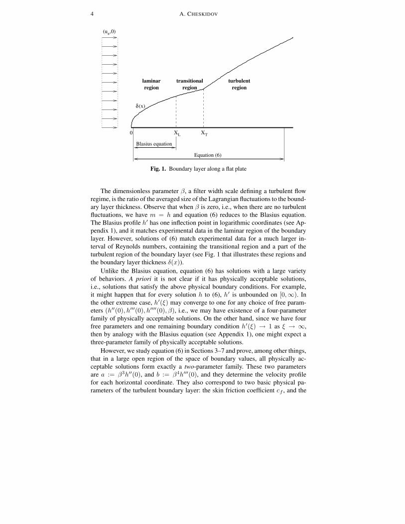
4 A. CHESKIDOV

0

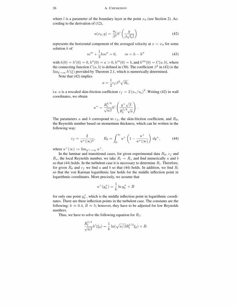
regiontransitional turbulent

regionlaminarregion

Equation (6)

Blasius equation

XTXL

δ(x)

(ue,0)

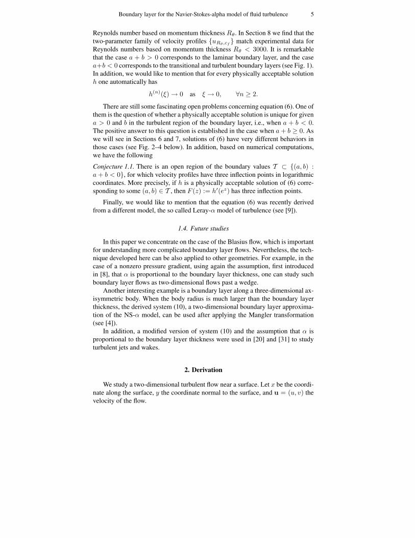
Fig. 1. Boundary layer along a flat plate

The dimensionless parameter β, a filter width scale defining a turbulent flowregime, is the ratio of the averaged size of the Lagrangian fluctuations to the bound-ary layer thickness. Observe that when β is zero, i.e., when there are no turbulentfluctuations, we have m = h and equation (6) reduces to the Blasius equation.The Blasius profile h′ has one inflection point in logarithmic coordinates (see Ap-pendix 1), and it matches experimental data in the laminar region of the boundarylayer. However, solutions of (6) match experimental data for a much larger in-terval of Reynolds numbers, containing the transitional region and a part of theturbulent region of the boundary layer (see Fig. 1 that illustrates these regions andthe boundary layer thickness δ(x)).

Unlike the Blasius equation, equation (6) has solutions with a large varietyof behaviors. A priori it is not clear if it has physically acceptable solutions,i.e., solutions that satisfy the above physical boundary conditions. For example,it might happen that for every solution h to (6), h′ is unbounded on [0,∞). Inthe other extreme case, h′(ξ) may converge to one for any choice of free param-eters (h′′(0), h′′′(0), h′′′′(0), β), i.e., we may have existence of a four-parameterfamily of physically acceptable solutions. On the other hand, since we have fourfree parameters and one remaining boundary condition h′(ξ) → 1 as ξ → ∞,then by analogy with the Blasius equation (see Appendix 1), one might expect athree-parameter family of physically acceptable solutions.

However, we study equation (6) in Sections 3–7 and prove, among other things,that in a large open region of the space of boundary values, all physically ac-ceptable solutions form exactly a two-parameter family. These two parametersare a := β3h′′(0), and b := β4h′′′(0), and they determine the velocity profilefor each horizontal coordinate. They also correspond to two basic physical pa-rameters of the turbulent boundary layer: the skin friction coefficient cf , and the


Reynolds number based on momentum thickness Rθ. In Section 8 we find that thetwo-parameter family of velocity profiles uRθ,cf match experimental data forReynolds numbers based on momentum thickness Rθ < 3000. It is remarkablethat the case a + b > 0 corresponds to the laminar boundary layer, and the casea+b < 0 corresponds to the transitional and turbulent boundary layers (see Fig. 1).In addition, we would like to mention that for every physically acceptable solutionh one automatically has

h(n)(ξ)→ 0 as ξ → 0, ∀n ≥ 2.

There are still some fascinating open problems concerning equation (6). One ofthem is the question of whether a physically acceptable solution is unique for givena > 0 and b in the turbulent region of the boundary layer, i.e., when a + b < 0.The positive answer to this question is established in the case when a+ b ≥ 0. Aswe will see in Sections 6 and 7, solutions of (6) have very different behaviors inthose cases (see Fig. 2–4 below). In addition, based on numerical computations,we have the following

Conjecture 1.1. There is an open region of the boundary values T ⊂ (a, b) :a+ b < 0, for which velocity profiles have three inflection points in logarithmiccoordinates. More precisely, if h is a physically acceptable solution of (6) corre-sponding to some (a, b) ∈ T , then F (z) := h′(ez) has three inflection points.

Finally, we would like to mention that the equation (6) was recently derivedfrom a different model, the so called Leray-α model of turbulence (see [9]).

1.4. Future studies

In this paper we concentrate on the case of the Blasius flow, which is importantfor understanding more complicated boundary layer flows. Nevertheless, the tech-nique developed here can be also applied to other geometries. For example, in thecase of a nonzero pressure gradient, using again the assumption, first introducedin [8], that α is proportional to the boundary layer thickness, one can study suchboundary layer flows as two-dimensional flows past a wedge.

Another interesting example is a boundary layer along a three-dimensional ax-isymmetric body. When the body radius is much larger than the boundary layerthickness, the derived system (10), a two-dimensional boundary layer approxima-tion of the NS-α model, can be used after applying the Mangler transformation(see [4]).

In addition, a modified version of system (10) and the assumption that α isproportional to the boundary layer thickness were used in [20] and [31] to studyturbulent jets and wakes.

2. Derivation

We study a two-dimensional turbulent flow near a surface. Let x be the coordi-nate along the surface, y the coordinate normal to the surface, and u = (u, v) thevelocity of the flow.

6 A. CHESKIDOV

We will use the two dimensional Navier-Stokes-α model to study the averagedvelocity in the boundary layer. This model is written as

∂∂tv + (u · ∇)v + vj∇uj = ν∆v −∇q∇ · u = 0,

(7)

where u = (u, v) represents the averaged velocity, and

v = u− ∂

∂xi

(α2δij

∂

∂xju

).

We supplement the system with no-slip boundary conditions u|y=0 = 0, as wellas

limy→∞

u(x, y) = (Ue(x), 0),

for all x > 0, where (Ue(x), 0) is an averaged external velocity of the flow. Inaddition, we assume that α(·) is a function of x only. If the averaged velocity u isstationary in time, (7) becomes

u(x, y) ∂∂xγ(x, y) + v ∂

∂yγ + γ ∂∂xu+ τ ∂

∂xv = ν ∂2

∂x2 γ + ν ∂2

∂y2 γ − ∂∂xq

u(x, y) ∂∂xτ(x, y) + v ∂

∂y τ + γ ∂∂yu+ τ ∂

∂yv = ν ∂2

∂x2 τ + ν ∂2

∂y2 τ − ∂∂y q

∂∂xu+ ∂

∂y v = 0.

(8)

Let us fix l on the x-axis, and define ue := Ue(l) and

ε(l) :=1√Rl

=

√ν

uel.

We change variables:

x1 =x

l, y1 =

y

εl, u1 =

u

ue, v1 =

v

εue, q1 =

q

u2e

, α1 =α

εl.

Note that the new variables are dimensionless. Recall that α1(·) is a function of x.Then we obtain

1

ueγ(x, y) = u1(x1, y1)− ε2α2

1

∂2

∂x21

u1 − α21

∂2

∂y21

u1 − ε2∂

∂x1α2

1 ·∂

∂x1u1,

1

ueτ(x, y) = εv1(x1, y1)− ε3α2

1

∂2

∂x21

v1 − εα21

∂2

∂y21

v1 − ε3∂

∂x1α2

1 ·∂

∂x1v1.

Neglecting the terms in equation (8) with high powers of ε, dropping subscriptsand denoting

w =

(1− α2 ∂

2

∂y2

)u,

we arrive at

u ∂∂xw + v ∂

∂yw + w ∂∂xu = ∂2

∂y2w − ∂∂xq

w ∂∂yu = − ∂

∂y q∂∂xu+ ∂

∂y v = 0.

(9)


Now we introduce the expression for the averaged pressure p in the boundary layerin terms of the pressure analog q:

p(x, y) := q +1

2u2 − 1

2α2

(∂

∂yu

)2

.

Note that the second equation in (9) implies that ∂∂yp = 0, which is consistent

with the fact that the variation of the averaged pressure in the vertical direction isnegligible within the boundary-layer approximation (see [4]). Therefore, assumingBernoulli’s equation U 2(x) + 2p(x) = const. for the rescaled external velocityU(x) = Ue(x)/ue, we deduce that

∂

∂xp(x, y) = U(x)U ′(x).

Finally, rewriting equations (9) in terms of p, we obtain the following boundarylayer approximation of the NS-α model:

u ∂∂xw + v ∂

∂yw + z(u) = ∂2

∂y2w − ∂∂xp

∂∂xu+ ∂

∂y v = 0

w = u− α2 ∂2

∂y2u,

(10)

where

z(u) = α2

(∂u

∂y

∂2u

∂x∂y− ∂u

∂x

∂2u

∂y2

)+

1

2

∂

∂xα2 ·

(∂

∂yu

)2

.

For ε small enough we have

u(x, y) ≈ ueu∞

(x

l,

y√l · le

), v(x, y) ≈ ue√

Rlv∞

(x

l,

y√l · le

),

where le is a length associated with the external flow le = ν/ue and (u∞, v∞) isa solution of (10).

When α = 0, the system (10) reduces to the Prandtl equations (1) modulorescaling. Our aim is to solve this system in the case of a zero pressure gradientflow along a flat plate. We will study the flow near some fixed point x0 on theplate. Let us choose the origin on the plate so that the point x0 has the coordinates(l, 0), and consider l is to be a parameter of the boundary layer at point x0. Now,we assume that α is proportional to

√x, i.e.,

α =√xβ,

where β is another parameter of the boundary layer defining a turbulent flowregime, which represents the ratio of the averaged size of the Lagrangian fluc-tuations to the boundary layer thickness. In addition, we will study the solutions(u∞, v∞) of (10) such that

u∞ = f(ξ), v∞ =1√xg(ξ), ξ =

y√x

(11)

8 A. CHESKIDOV

for some functions f and g on an adequate interval l − ε < x < l + ε. It isremarkable that the self-similarity assumption (11) yields z(u∞) ≡ 0.

Substituting the expressions (11) for u and v into (10), and setting ∂∂xp = 0,

we obtain the following equations for f and g:− 1

2ff′ξ + β2f( 1

2f′′′ξ + f ′′)− β2ff ′′ + gf ′ − β2f ′′′g = f ′′ − β2f ′′′′

g′ − 12ξf

′ = 0.

Let

h(ξ) =

∫ ξ

0

f(η) dη.

Then g = 12ξh′ − 1

2h, and we have the following equation for h:

h′′′ +1

2hh′′ − β2

(h′′′′′ +

1

2h′′′′)

= 0. (12)

The boundary condition u|y=0 = 0 requires f(0) = 0 and thus h(0) = h′(0) = 0.In addition, the physical interpretation of ν ∂

∂yu for y = 0 as the shear stress on thewall imposes the condition f ′(0) > 0, that is, h′′(0) > 0. Moreover, u(x, y)→ ue

as y →∞ requires that h′(ξ)→ 1 as ξ →∞.Note that if h(ξ) is a solution of (12), then h(x) := βh(βx) is a solution of

−h′′′′′ − 1

2hh′′′′ + h′′′ +

1

2hh′′ = 0. (13)

This equation can be also written asm′′′ + 1

2hm′′ = 0

m = h− h′′. (14)

The physical boundary conditions are h(0) = h′(0) = 0, h′′(0) > 0, and h′(x)→β2 as x→∞.

Note that the last boundary condition is equivalent to the condition that limx→∞ h′(x)exists and satisfies

0 < limx→∞

h′(x) <∞. (15)

In this case h is a solution to our boundary value problem with β defined as

β :=(

limx→∞

h′(x))1/2

.

Recall that β = α(x)/√x, and a priori we do not know how to choose this physi-

cal parameter. By finding a solution h subjected to the condition (15), we will alsofind the value of the parameter β.

As we already discussed in Introduction, we have a fifth-order nonlinear ordi-nary differential equation, and since h(0) = h′(0) = 0, we have to specify threeboundary conditions (h′′(0), h′′′(0), h′′′′(0)) in order to solve it. In Sections 3–7we will prove that given a pair (h′′(0), h′′′(0)) in a large adequate region, there isa right choice of h′′′′(0) that guarantees (15), i.e., there is a two-parameter familyof physically acceptable solutions. More precisely, we prove the following


Theorem 2.1. There exists a continuous function b0 : (0,∞) → R such thatb0(a) < −a, and for each a > 0 and b ∈ (b0(a),∞) we have that limx→∞ h′(x)exists and satisfies

0 < limx→∞

h′(x) <∞,

where h(x) is a solution to (13) with h(0) = h′(0) = 0, h′′(0) = a, h′′′(0) = b,and h′′′′(0) = C(a, b). The function C(a, b) is defined in Section 5.

We also show that the condition b ∈ (b0(a),∞) cannot be removed, i.e., thereare no physically acceptable solutions for some choices of (h′′(0), h′′′(0)) in theregion where h′′(0)+h′′′(0) < 0 and |h′′(0)+h′′′(0)| is large enough (see Corol-lary 7.6).

Here is a brief outline of the strategy to prove Theorem 2.1. In Section 3 weclassify solutions of (13) and characterize their properties (see Theorem 3.1). InSection 4 we show how the different types of solutions depend upon the boundaryconditions. In Section 5 we define a functionC(a, b), which we call the connectingfunction, and study its properties. This function connects the boundary values ofthe physically acceptable solutions:

h′′′′(0) = C(h′′(0), h′′′(0)), (16)

as we show in Sections 6 and 7. In Section 6 we prove that in the case h′′(0) +h′′′(0) ≥ 0, h is physically acceptable if and only if (16) holds (Theorem 6.3). InSection 7 we show that in the case h′′(0) + h′′′(0) < 0, when |h′′(0) + h′′′(0)|is not large, (16) implies that h is physically acceptable (Theorem 7.3). When|h′′(0) + h′′′(0)| is large enough, physically acceptable solutions might not exists(Corollary 7.6).

3. Classification of the solutions of (13)

Let h(x) be a solution of (13). The first equation in (14) implies that

m′′(x) = m′′(0)e−12

R x0h(y) dy. (17)

Since m′′ has a constant sign, m′ is monotonic and therefore the integral

I(h) :=

∫ x∗

0

e−xm′(x) dx,

where [0, x∗) is the maximal existence interval of the solution, makes sense pro-vided the values ±∞ are also accepted.

The following is a characterization of the behavior of the solutions for x→∞.

Theorem 3.1. Let h(x) be a solution of (13) with h(0) = 0, h′(0) = 0, h′′(0) > 0.Then only the following four cases are possible:

1. x∗ =∞, I(h) < h′′(0), m′(x)→ γ ∈ R, and h′(x)→∞ as x→∞.2. x∗ =∞, I(h) = h′′(0), m′(x)→ γ ≥ 0, and h′(x)→ γ as x→∞.3. x∗ =∞, I(h) > h′′(0), m′′(0) = 0, and h′(x)→ −∞ as x→∞.

10 A. CHESKIDOV

4. I(h) > h′′(0), m′′(0) > 0, m′(x)→∞, and h′(x)→ −∞ as x→ x∗.

Proof. It is useful to consider first the particular case when m′′(0) = 0. In thiscase m′(x) = const =: γ, and elementary computations show that one of thecases 1, 2, or 3 occurs. From now on we will suppose that m′′(0) 6= 0.

Considerh′ − h′′′ = m′.

A general solution h′ has the following integral representation:

h′(x) =1

2

(ex − e−x

)h′′(0)− 1

2

∫ x

0

(ex−y − e−x+y

)m′(y) dy. (18)

Note that if I(h) is finite, then (18) implies that

2h′(x) − ex (h′′(0)− I(h))

= −e−xh′′(0) +

∫ x∗

x

ex−ym′(y) dy +

∫ x

0

e−x+ym′(y) dy. (19)

First, assume m′(x) → γ ∈ R as x → x∗. Then I(h) is finite. Suppose,x∗ <∞. Then (18) implies that h′ is bounded on [0, x∗). Thus h is also bounded.Since m′ = h′ − h′′′, it follows that h′′′ is bounded. Thus h′′ is bounded. Also,(17) implies that m′′ is bounded. However, m′′ = h′′ − h′′′′. Therefore h′′′′ isbounded. This contradicts the definition of x∗. Hence x∗ = ∞. Now (19) impliesthat

2h′(x)− ex (h′′(0)− I(h))→ 2γ as x→∞.If h′′(0) < I(h), then h′(x) → −∞ as x → ∞ and from (17) it follows that|m′′(x)| → ∞ as x → ∞. This contradicts the assumption that m′(x) → γ ∈ Ras x → ∞. Thus we have concluded that if this latter condition holds, then eithercase 1 or case 2 occurs.

Second, assume that m′(x) → −∞ as x → x∗. If x∗ < ∞, then (18) impliesthat h′(x) is bounded from below on [0, x∗). However, since lim infx→x∗ m

′′(x) =−∞, from (17) we conclude that lim infx→x∗

∫ x0h(y) dy = −∞. This implies

that h′ is not bounded from below, a contradiction. Therefore x∗ = ∞ and sinceh′′(0) > 0, (18) implies that h′(x)→∞. Thus, by (17),m′′(x) goes to zero fasterthan an exponential function, so that m′(x) is bounded on [0,∞), a contradiction.Hence m′(x) has to be bounded from below on [0, x∗).

Third, assume that m′(x) → ∞ as x → x∗ and x∗ < ∞. Since we havethat lim supx→x∗ m

′′(x) =∞, we get lim infx→x∗∫ x

0h(y) dy = −∞ (see (17)),

which implies that h′(x) is not bounded from below. If

I(h) ≤ h′′(0),

then, in particular, I(h) is finite and consequently (19) implies that

2h′(x) ≥ −e−xh′′(0) +

∫ x∗

x

ex−ym′(y) dy +

∫ x

0

e−x+ym′(y) dy.


Thus h′ is bounded from below, a contradiction. Hence

I(h) > h′′(0).

Since m′′ has a constant sign (see (17)), we have m′′(0) > 0 and m′′(x) > 0on [0, x∗). It follows that

∫ x0

(ex−y − e−x+y)m′′(y) dy is nonnegative on [0, x∗).Note that the general solution of h′′ − h′′′′ = m′′ is

2h′′(x) =(ex − e−x

)h′′′(0)+

(ex + e−x

)h′′(0)−

∫ x

0

(ex−y − e−x+y

)m′′(y) dy.

Thus h′′(x) is bounded from above on [0, x∗). This and the fact that h′ is un-bounded from below force h′(x)→ −∞ as x→ x∗. Therefore case 4 occurs.

The last case to be considered is when m′(x)→∞ as x→∞. If

I(h) ≤ h′′(0),

then, in particular, I(h) is finite and consequently (19) implies that

2h′(x) ≥ −e−xh′′(0) +

∫ ∞

x

ex−ym′(y) dy +

∫ x

0

e−x+ym′(y) dy →∞

as x → ∞. But in this case from (17) it follows that m′ has to be bounded, acontradiction. Hence

I(h) > h′′(0).

Let x0 := infx : x > 0,m′(x) > 0. Then for each x ≥ 2x0 we have thefollowing inequality:

∫ x

x0

(e−y − e−2x+y

)m′(y) dy ≥

∫ x/2

x0

(e−y − e−2x+y

)m′(y) dy

≥(1− e−x

) ∫ x/2

x0

e−ym′(y) dy.

Therefore from (18) we obtain that for x ≥ 2x0

2h′(x)e−x ≤ h′′(0)−∫ x

0

(e−y − e−2x+y

)m′(y) dy

≤ h′′(0)−∫ x0

0

e−ym′(y) dy −(1− e−x

) ∫ x/2

x0

e−ym′(y) dy

→ h′′(0)− I(h) < 0

as x→∞. Hence h′(x)→ −∞ as x→∞, which corresponds to case 4. ut

Fix a > 0 and b. For a given c let hc be a solution of (13) with hc(0) =h′c(0) = 0, h′′c (0) = a, h′′′c (0) = b, and h′′′′c (0) = c. Let also mc = hc − h′′c .

Recall that the physically acceptable solutions have to satisfy the followingboundary condition at infinity:

h′c(x)→ β2 as x→∞, (20)

12 A. CHESKIDOV

for some β > 0. By Theorem 3.1 such a solution has to fall in the second case,that is, I(hc) = a. Conversely, any solution from the second case has to satisfy(20) for some β > 0 except the non-generic case when the limit of h′c is zero.

We would like to know whether for given a and b there exists c such that hcis physically acceptable. To this aim we will study in more detail the four cases ofthe Theorem 3.1 in the next section.

4. Classification criteria

Lemma 4.1. If c > a, then hc is in one of the cases 1 or 2 in Theorem 3.1, i.e.,

I(hc) ≤ a.

Proof. Indeed, since c > a, the second equation in (14) implies that m′′(0) < 0and therefore cases 3 and 4 of the Theorem 3.1 are excluded. ut

We can supplement this lemma with the following

Lemma 4.2. For each a > 0 and b ∈ R there exists cl(a, b) such that hc is in oneof the cases 3 or 4 in Theorem 3.1, i.e,

I(hc) > a

for all c < cl(a, b).

Proof. Take any c < a. Assume that hc exists for all x ≥ 0. Note that sincem′′c (0) = a− c > 0, we have m′c(x) > m′c(0) for each x > 0. Therefore

∫ x

0

(ex−y − e−x+y

)m′c(y) dy ≥

(ex + e−x − 2

)m′c(0)

= −(ex + e−x − 2

)b

=: ψ1(b, x)

for each x ≥ 0. Hence, due to the integral representation (18) of h′c, we obtain

2h′c(x) ≤(ex − e−x

)h′′c (0)− ψ1(b, x)

=(ex − e−x

)a− ψ1(b, x).

=: ψ2(a, b, x)

for each x ≥ 0. Consequently

2hc(x) = 2

∫ x

0

h′c(y) dy ≤∫ x

0

ψ2(a, b, y) dy =: ψ3(a, b, x), x ≥ 0.

Thus, since m′′(0) = a− c > 0, we have that

m′′c (x) = m′′c (0)e−12

R x0hc(y) dy ≥ m′′c (0)e−

14

R x0ψ3(a,b,y) dy =: m′′c (0)ψ4(a, b, x)


for each x ≥ 0. Note that ψ4(a, b, x) does not depend on c, which is an essentialpart of this proof. Now we have the following inequality for m′c(x):

m′c(x) ≥ m′c(0) +m′′c (0)

∫ x

0

ψ4(a, b, y) dy, x ≥ 0.

Thus

I(hc) =

∫ ∞

0

e−xm′c(x) dx

≥∫ ∞

0

e−x(m′c(0) +m′′c (0)

∫ x

0

ψ4(a, b, y) dy

)dx (21)

= −b+ (a− c)Θa,b ,

where

Θa,b :=

∫ ∞

0

dx e−x∫ x

0

dy ψ4(a, b, y).

Since Θa,b ∈ (0,∞], we can define

cl(a, b) = min a, a− (a+ b)/Θa,b .

Take any c < cl(a, b). If the maximal existence interval of hc is finite (x∗ <∞), then Theorem 3.1 implies that I(hc) > a. If hc exists for all x ≥ 0, thenI(hc) > a by (21). ut

In addition, we have the following result:

Lemma 4.3. For any a > 0 and b < −a there exists cu(a, b) such that h′c(x) > 0for all x > 0, and h′c(x)→∞ as x→∞ for all c > cu(a, b).

In particular, hc is in the case 1 in Theorem 3.1, i.e.,

I(hc) < a

for all c > cu(a, b).

Proof. Differentiating (18), we obtain

2h′′c (x) =(ex + e−x

)a−

∫ x

0

(ex−y + e−x+y

)m′(y) dy. (22)

For c > a we have m′′c (x) < 0 for all x ≥ 0 (see (17)). This implies that m′c(x) ≤−b for all x ≥ 0. Therefore (22) implies that

2h′′c (x) ≥(ex + e−x

)a+ b

∫ y

0

(ex−y + e−x+y

)dy

=(ex + e−x

)a+

(ex − e−x

)b

for all x ≥ 0. Since a > 0, there exists x0, independent of c, such that h′′c (x) > 0for all c > a and 0 ≤ x ≤ x0.

14 A. CHESKIDOV

The next step is to prove that there exists cu such that

m′c(x0) < 0, ∀c > cu.

Choose cu > a such that

−b+ (a− c)∫ x0

0

e−14 (ex−e−x−2x)a dx < 0, ∀c > cu.

Choose any c > cu. Suppose that m′c(x) ≥ 0 for all x ∈ [0, x0]. Then∫ x

0

(ex−y − e−x+y

)m′c(y) dy ≥ 0, x ∈ [0, x0].

Therefore (18) forces

2h′c(x) ≤(ex − e−x

)a, x ∈ [0, x0],

which implies that

2hc(x) ≤(ex + e−x − 2

)a, x ∈ [0, x0].

Thus

m′′c (x) = (a− c)e− 12

R x0hc(y) dy ≤ (a− c)e− 1

4 (ex−e−x−2x)a, x ∈ [0, x0].

Finally,

m′c(x0) ≤ −b+ (a− c)∫ x0

0

e−14 (ex−e−x−2x)a dx < 0,

a contradiction. Hence m′c(x0) < 0.Consequently, since m′c(x) is decreasing, we have m′c(x) < 0 for all x ≥ x0.

Note that h′′′c (x0) = h′c(x0) − m′c(x0) > 0. We can show now that h′′′c (x) > 0for all x ≥ x0. Indeed, suppose that there exists x1 > x0 such that h′′′c (x) > 0on [x0, x1) and h′′′c (x1) = 0. Recall that h′′c (x) > 0 for all x ∈ [0, x0]. Thenh′c(x1) > 0, and, consequently, m′(x1) = h′c(x1)− h′′′c (x1) > 0, a contradiction.

Hence h′′c (x) > 0 and h′c(x) > 0 for all x > 0. In addition, noting thatlimx→∞m′c(x) < 0, we conclude from Theorem 3.1 that h′c(x)→∞ as x→∞.ut

Lemma 4.4. If I(hc) ≤ a for some c ≤ a, then I(hc) < a for all c < c ≤ a. IfI(hc) ≥ a for some c ≤ a, then I(hc) > a for all c < c.

Proof. Let c1 < c2 ≤ a. Since h′′′′c1 (0) < h′′′′c2 (0), then h′c1(x) < h′c2(x) forx > 0 small enough. Suppose there exists x0 that belongs to the existence intervalsof both hc1 and hc2 such that h′c1(x0) = h′c2(x0) and h′c1(x) < h′c2(x) for 0 <x < x0. Since m′′c1(0) > m′′c2(0) ≥ 0, (17) implies that m′′c1(x) > m′′c2(x) for0 < x < x0. Thereforem′c1(x) > m′c2(x) for 0 < x < x0. Comparing the integralrepresentations (18) of h′c1 and h′c2 , we obtain h′c1(x0) < h′c2(x0), a contradiction.

Hence h′c1(x) < h′c2(x) and consequently m′c1(x) > m′c2(x) for each x thatbelongs to the existence intervals of both hc1 and hc2 . This, together with thedefinition of I(h) and Theorem 3.1, completes the proof. ut


5. Connecting function

The aim of this section is to introduce and study several regions in the space ofthe boundary values a, b, and c, which are useful in the study of the existence of aphysically acceptable solution. The following result will play an essential role inthis study.

Denote by ha,b,c the solution of (13) with ha,b,c(0) = h′a,b,c(0) = 0, h′′a,b,c(0) =a > 0, h′′′a,b,c(0) = b, and h′′′′a,b,c(0) = c. Whenever a and b are fixed, we will usefor simplicity our previous notation hc = ha,b,c.

Proposition 5.1. Let

Ω := (a, b, c) : a > 0, I(ha,b,c) < a,

Ω0 := Ω ∩ (a, b, c) : h′a,b,c(x) > 0 ∀x > 0.Then Ω and Ω0 are open in R3.

Proof. Choose any (a, b, c) ∈ Ω. Let h = ha,b,c and m := h− h′′. Write

δ := a− I(h) > 0.

By Theorem 3.1, the maximal existence interval of h is infinite. Moreover, m′(x)→γ as x→∞ for some γ ∈ R. Since

∫ ∞

x

ex−ym′(y) dy +

∫ x

0

e−x+ym′(y) dy → 2γ

as x→∞, we can choose x so that∫ ∞

x

ex−ym′(y) dy +

∫ x

0

e−x+ym′(y) dy > 2γ − 1, ∀x ≥ x. (23)

Since h′(x)→∞ (see Theorem 3.1), we have that h(x)→∞, and, consequently,

limx→∞

m′′(x)

h(x)= 0.

Therefore we can choose x0 > x, such that h(x0) > 0 and h′(x) > 0 for allx ≥ x0, as well as

|m′′(x0)|h(x0)

<δ

32,

δ

2ex0 > a− 2γ + 2. (24)

Continuous dependence on the initial data implies that there exists ε0 ∈ (0, δ/4)such that any solution h of (13) with the boundary values satisfying

|h(n)(0)− h(n)(0)| < ε0, n = 0, ..., 4,

exists on [0, x0] and satisfies the following conditions:

h(x0) > 0, h′(x0) > 0,|m′′(x0)|h(x0)

<δ

32,

16 A. CHESKIDOV

and

|m′(x)− m′(x)| < δ

8, ∀x ∈ [0, x0].

If there exists x ∈ (0, x0] such that h′(x) ≤ 0, define ε = ε0. In the opposite casewhen h′(x) > 0 for all x > 0, choose ε ∈ (0, ε0) small enough that h′(x) > 0 on(0, x0] for all solutions h with boundary values satisfying

|h(n)(0)− h(n)(0)| < ε, n = 0, ..., 4. (25)

This can be done because h′′(0) = a > 0.We now fix any solution h satisfying (25). Let [0, x∗) be the maximal existence

interval of h. Define

x1 := supx : x ≤ x∗, h′(x) > 0 on [x0, x)

Then (17) implies that for any x ∈ [x0, x1) we have

|m′′(x)| ≤ |m′′(x0)|e− 12 (x−x0)h(x0).

Therefore

|m′(x)−m′(x0)| ≤ 2|m′′(x0)|h(x0)

(1− e− 1

2 (x−x0)h(x0))

≤ 2|m′′(x0)|h(x0)

<δ

16

for all x ∈ [x0, x1). Similarly, |m′(x)−m′(x0)| < δ/16 for all x ∈ [x0, x1). Thuswe have

|m′(x)− m′(x)| < |m′(x0)− m′(x0)|+ δ

8<δ

4, x ∈ [x0, x1).

Hence (see (18))

2|h′(x)− h′(x)| ≤(ex − e−x

)ε+

∫ x

0

(ex−y − e−x+y

)|m′(y)− m′(y)| dy

<δ

4ex +

δ

4

(ex + e−x − 2

)(26)

<δ

2ex

for all x ∈ [x0, x1). On the other hand, from (19) and (23) it follows that

2h′(x) = ex(a− I(h)

)− e−xa+

∫ ∞

x

ex−ym′(y) dy +

∫ x

0

e−x+ym′(y) dy

> δex − a+ 2γ − 1


for all x ∈ [x0, x1). This, together with (26) and (24), allows us to conclude that

2h′(x) >δ

2ex − a+ 2γ − 1 > 1, x ∈ [x0, x1). (27)

Assume now that x1 < x∗. Since h′ is continuous, by the definition of x1 wehave h′(x1) = 0. On the other hand, (27) implies that h′(x1) ≥ 1, a contradiction.Thus x1 = x∗. Therefore h′(x) does not converge to −∞ when x x∗, and,consequently, from Theorem 3.1 we must have x∗ =∞. Then (27) yields

limx→∞

h′(x) =∞,

i.e., I(h) < a, according to Theorem 3.1. Moreover, h′(x) > 0 on the wholeinterval [x0,∞).

The second part of the proposition follows from the fact that in the case underconsideration h′(x) > 0 on (0, x0]. ut

Among all the solutions hc consider the special solution ha. From (18) it fol-lows that

2h′a(x) = (a+ b)ex − (a− b)e−x − 2b, I(ha) = −b. (28)

We have two major cases. If a + b ≥ 0, then we have I(ha) ≤ a. If a + b < 0,then I(ha) > a. In addition, from Lemma 4.4 we deduce that

I(hc) > a for b < −a < 0, c ≤ a. (29)

Let

Λ := (a, b) : ∃c such that (a, b, c) ∈ Ω0.

Define the connecting function C : Λ→ R by

C(a, b) := infc : (a, b, c) ∈ Ω0. (30)

For convenience (a, b, C(a, b) will be called the connecting surface.

Lemma 5.2. We have

Λ = (0,∞)× (−∞,∞).

In addition, (a,−a, c) ∈ Ω0 for all c > a > 0, and

a < C(a, b) <∞, if a+ b < 0,

C(a, b) = a, if a+ b = 0,

−∞ < C(a, b) < a, if a+ b > 0.

18 A. CHESKIDOV

Proof. First, if a+ b < 0, then Lemma 4.3 implies that there exists c large enoughthat h′c(x) > 0 for all x > 0 and h′c(x)→∞ as x→∞. Therefore (a, b) ∈ Λ andC(a, b) <∞. In addition, (29) implies that C(a, b) ≥ a. Moreover, since h′a(x) isnegative for some x > 0 (see (28)), we have C(a, b) > a by virtue of continuousdependence on the initial data.

Second, if a + b > 0, then h′a(x) > 0 for all x > 0, and h′a(x) → ∞ asx → ∞, i.e., (a, b, a) ∈ Ω0. Therefore (a, b) ∈ Λ and C(a, b) ≤ a. Moreover,since Ω0 is open, we obtain (a, b, C(a, b)) /∈ Ω0, and consequently C(a, b) < a.In addition, from Lemma 4.2 we infer that C(a, b) > −∞.

Now note that (17) yields m′′c (x) < 0 for all c > a, all x > 0. Therefore

m′c(x) < m′c(0) = −b = m′a(x), c > a, x > 0. (31)

Hence,

I(hc) =

∫ ∞

0

e−ym′c(y) dy < m′c(0) = −b, c > a.

Thus, if a + b = 0, we get that I(hc) < a for all c > a, and consequently byTheorem 3.1 we have h′c(x) → ∞ as x → ∞ for all c > a. In addition, we geth′c(x) > h′a(x) > 0 for all c > a and x > 0 due to (18) and (31). Therefore,(a,−a, c) ∈ Ω0 for all c > a. Hence (a,−a) ∈ Λ, and C(a,−a) ≤ a. SinceI(ha) = a we obtain C(a,−a) = a due to Lemma 4.4. ut

Lemma 5.3. The function C(a, b) is upper semi-continuous for all a > 0 andb ∈ R.

Proof. Notice that the set Ω0 is open due to Theorem 5.1. Thus the set

(a, b, c) : a > 0, c > C(a, b) =⋃

p>0

(Ω0 + (0, 0, p))

is open. Therefore C(a, b) is upper semi-continuous. ut

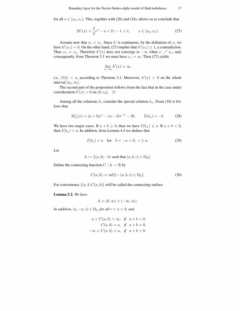
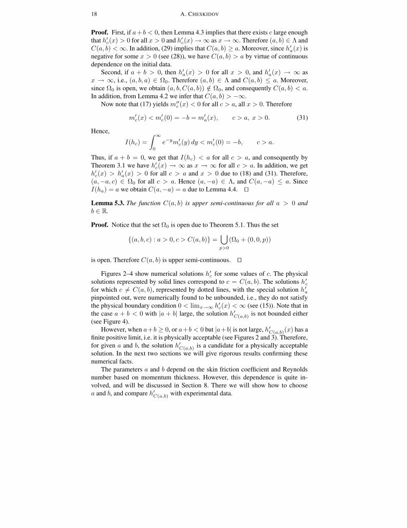
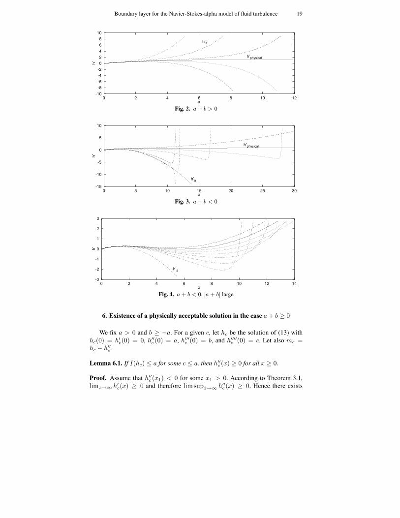
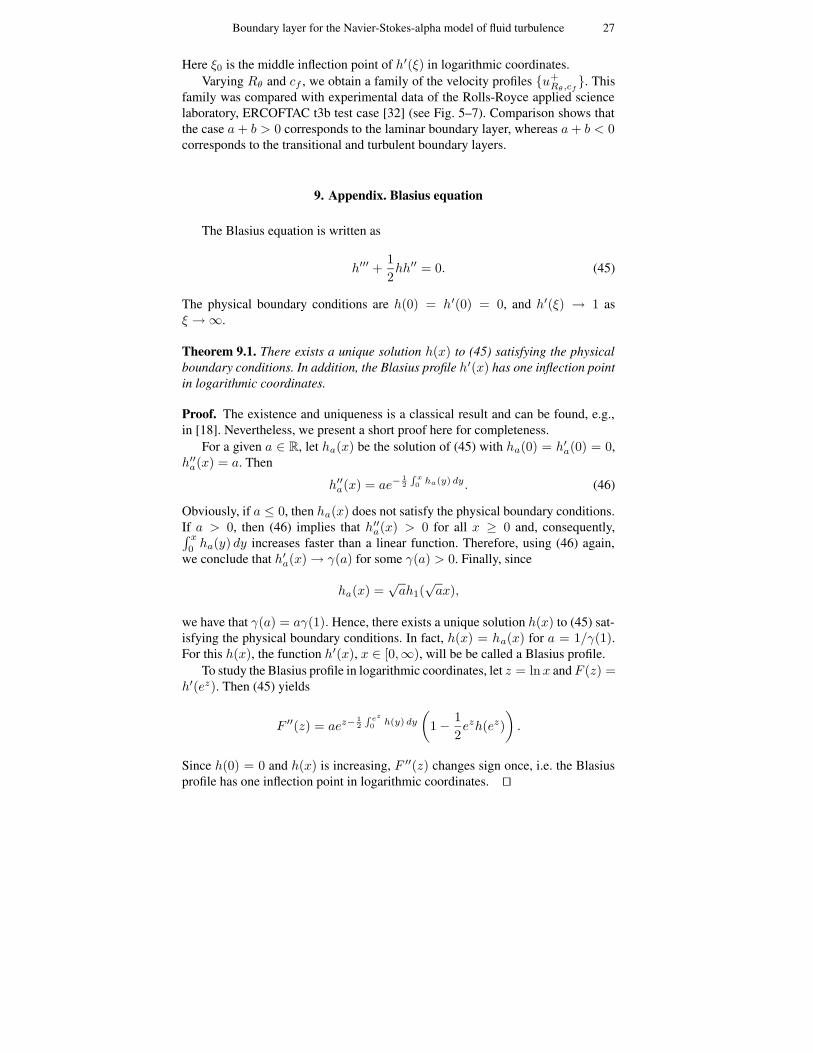
Figures 2–4 show numerical solutions h′c for some values of c. The physicalsolutions represented by solid lines correspond to c = C(a, b). The solutions h′cfor which c 6= C(a, b), represented by dotted lines, with the special solution h′apinpointed out, were numerically found to be unbounded, i.e., they do not satisfythe physical boundary condition 0 < limx→∞ h′c(x) <∞ (see (15)). Note that inthe case a + b < 0 with |a + b| large, the solution h′C(a,b) is not bounded either(see Figure 4).

However, when a+b ≥ 0, or a+b < 0 but |a+b| is not large, h′C(a,b)(x) has afinite positive limit, i.e. it is physically acceptable (see Figures 2 and 3). Therefore,for given a and b, the solution h′C(a,b) is a candidate for a physically acceptablesolution. In the next two sections we will give rigorous results confirming thesenumerical facts.

The parameters a and b depend on the skin friction coefficient and Reynoldsnumber based on momentum thickness. However, this dependence is quite in-volved, and will be discussed in Section 8. There we will show how to choosea and b, and compare h′C(a,b) with experimental data.


-10-8-6-4-202468

10

0 2 4 6 8 10 12h’

x

h’a

h’physical

Fig. 2. a+ b > 0

-15

-10

-5

0

5

10

0 5 10 15 20 25 30

h’

x

h’a

h’physical

Fig. 3. a+ b < 0

-3

-2

-1

0

1

2

3

0 2 4 6 8 10 12 14

h’

x

h’a

Fig. 4. a+ b < 0, |a+ b| large

6. Existence of a physically acceptable solution in the case a+ b ≥ 0

We fix a > 0 and b ≥ −a. For a given c, let hc be the solution of (13) withhc(0) = h′c(0) = 0, h′′c (0) = a, h′′′c (0) = b, and h′′′′c (0) = c. Let also mc =hc − h′′c .

Lemma 6.1. If I(hc) ≤ a for some c ≤ a, then h′′c (x) ≥ 0 for all x ≥ 0.

Proof. Assume that h′′c (x1) < 0 for some x1 > 0. According to Theorem 3.1,limx→∞ h′c(x) ≥ 0 and therefore lim supx→∞ h′′c (x) ≥ 0. Hence there exists

20 A. CHESKIDOV

x2 > x1 such that h′′c (x2) > h′′c (x1). Consequently, since

h′′c (0) = a > 0 > h′′c (x1),

a local minimum of h′′c is attained at some x0 ∈ (0, x2). Then h′′c (x0) < 0 andh′′′′c (x0) ≥ 0. This implies that m′′c (x0) < 0. However, since c ≤ a, we have thatm′′c (x) ≥ 0 for all x > 0, a contradiction. Therefore h′′c (x) ≥ 0 for all x > 0. ut

Lemma 6.2. The set

(Ω \ Ω0) ∩ (a, b, c) : a+ b ≥ 0, c ≤ a

is empty.

Proof. Assume that (a, b, c) ∈ Ω, a + b ≥ 0, and c ≤ a. Since I(hc) < a andc ≤ a, Lemma 6.1 implies that h′′c (x) ≥ 0 for all x ≥ 0. Since h′c(0) = 0 andh′′c (0) = a > 0, we have that h′c(x) > 0 for all x > 0. Therefore (a, b, c) ∈ Ω0.ut

Theorem 6.3. If a > 0 and a+ b ≥ 0, then hC(a,b) is physically acceptable, i.e.,

limx→∞

h′C(a,b)(x) = γ (32)

for some γ = γ(a, b) ∈ (0,∞). In addition, h′′C(a,b)(x) ≥ 0 for all x > 0, C(a, b)

is continuous and strictly less than a for a+ b > 0, and C(a,−a) = a, Moreover,the physically acceptable solution hC(a,b) is unique, i.e.,

I(hc) 6= a, ∀c 6= C(a, b).

Proof. First, if a+ b = 0, then from (28) it follows that I(ha) = a and h′′a(x) ≥ 0for all x ≥ 0. Since C(a,−a) = a (see Lemma 5.2), (32) holds due to Theo-rem 3.1.

Assume now that a + b > 0. Let C = C(a, b). Note that C < a by virtue ofLemma 5.2. Since Ω0 is open, (a, b, C) /∈ Ω0. Therefore Lemma 6.2 yields

(a, b, C) /∈ Ω

Hence I(hC) ≥ a by the definition of Ω. Assume that I(hC) > a. Then Theo-rem 3.1 yields that

(a, b, C) ∈ Θ := (a, b, c) : a > 0, a+ b > 0, c < a, h′c(x) < 0 for some x > 0,

which is an open set by virtue of continuous dependence on the initial data. Nowrecall that the connecting surface belongs to the closure of Ω0. On the other hand,since Ω0 ∩Θ = ∅, we obtain that (a, b, C) does not belong to the closure of Ω0, acontradiction. Therefore I(hC) = a.

In addition, Lemma 4.4 implies that I(hc) > a for all c < C(a, b), andI(hc) < a for all C(a, b) < c ≤ a. Therefore, to show uniqueness of the physi-cally acceptable solution we have to prove that I(hc) 6= a for c > a. Indeed, dueto (17), m′′c (x) < 0 for all c > a, all x ≥ 0. Consequently, by the definition of


I(h), we have I(hc) < m′c(0) = −b ≤ a for c > a. The following is a summaryof what was proved so far:

I(hc) < a for c > C(a, b),

I(hc) = a for c = C(a, b),

I(hc) > a for c < C(a, b).

In particular, by Theorem 3.1 and Lemma 6.1 we have

(a, b, c) : a > 0, a+ b > 0, c < C(a, b) = Θ,

which is an open set, as we argued above. So, C(a, b) is lower semi-continuousfor a > 0, a+ b > 0. Combining this with Theorem 5.3 we obtain that C(a, b) isa continuous function for a > 0 and a+ b > 0. ut

7. Existence of a physically acceptable solution in the case a+ b < 0

For given a > 0, b < −a and c ∈ R, let ha,b,c be the solution of (13) withha,b,c(0) = h′a,b,c(0) = 0, h′′a,b,c(0) = a, h′′′a,b,c(0) = b, h′′′′a,b,c(0) = c. Let alsoma,b,c = ha,b,c − h′′a,b,c.

Due to (29), I(ha,b,c) > a for all b < −a, c ≤ a. So, in order to obtaina physically acceptable solution, we should concentrate on the case c > a, i.e.,when m′′a,b,c(0) < 0 (see (17)). Lemma 4.1 yields that I(ha,b,c) ≤ a in this case.In particular, this implies that ha,b,c is defined on [0,∞) (see Theorem 3.1).

LetΓ = (a, b, c) : a > 0, c = C(a, b),

i.e., Γ is the connecting surface (see Section 5). We start with the following

Lemma 7.1. Define γ : Γ→ R by

γ(a, b, c) = limx→∞

m′a,b,c(x).

Then γ is continuous at any point (a, b, c) ∈ Γ such that γ(a, b, c) > 0.

Proof. The definition of Γ and continuous dependence on the initial data implythat

h′a,b,c(x) ≥ 0, ∀(a, b, c) ∈ Γ, ∀x > 0. (33)

Take any (a, b, c) ∈ Γ such that γ(a, b, c) > 0. Let h := ha,b,c and m := ma,b,c.

Suppose that limx→∞ h′(x) = 0. Then, according to Theorem 3.1, γ(a, b, c) = 0,a contradiction. Therefore, by (33), we obtain limx→∞ h′(x) > 0. Thus we have(see (17))

h(x)→∞, m′′(x)→ 0 as x→∞.Given ε > 0, choose x0 large enough that

h(x) > 1, |m′′(x)| < ε

8, ∀x ≥ x0.

22 A. CHESKIDOV

The continuous dependence on the initial data implies that there exists a neighbor-hood N of (a, b, c) in Γ such that for any h = ha,b,c and m = ma,b,c, with theinitial data (a, b, c) ∈ N , we have

h(x0) > 1, |m′′(x0)| < ε

8, |m′(x0)− m′(x0)| < ε

2.

In addition, by virtue of (33), we obtain

h(x) > 1, x ≥ x0.

Hence, using (17), we derive that

|m′′(x)| = |m′′(x0)|e−12

R xx0h(y) dy

< |m′′(x0)|e− 12 (x−x0) <

ε

8e−

12 (x−x0)

for all x ≥ x0. Similarly,

|m′′(x)| < ε

8e−

12 (x−x0), x ≥ x0.

Thus

|m′(x)− m′(x)| < |m′(x0)− m′(x0)|+ 2

∫ x

x0

ε

8e−

12 (x−x0) dx <

ε

2+ε

2= ε

for all x ≥ x0. Consequently,

|γ(a, b, c)− γ(a, b, c)| ≤ ε.

This concludes the proof of the lemma. ut

Lemma 7.2. If γ(a, b, c) ≥ 0 for some (a, b, c) ∈ Γ such that a+ b < 0, then

I(ha,b,c) = a,

andlimx→∞

h′a,b,c(x) = γ(a, b, c).

Proof. Take any (a, b, c) ∈ Γ such that a+ b < 0. Lemma 5.2 implies that c > aand, consequently, I(ha,b,c) ≤ a due to Lemma 4.1. Assume that I(ha,b,c) < a,i.e., h′a,b,c(x)→∞ as x→∞ (see Theorem 3.1). Since Ω0 is open, Γ ∩ Ω0 = ∅,and we have that (a, b, c) /∈ Ω0. Thus, by the definition of Ω0, h′a,b,c(x0) = 0 forsome x0 > 0. Note that we also have h′a,b,c(0) = 0 and h′′a,b,c(0) = a > 0. Thusthe minimum of h′a,b,c is attained for some x1 > 0. Then we have h′a,b,c(x1) ≤ 0and h′′′a,b,c(x1) ≥ 0. Consequently, we obtain that

m′a,b,c(x1) = h′a,b,c(x1)− h′′′a,b,c(x1) ≤ 0.

Since c > a, we have that m′′a,b,c(x) < 0 for all x ≥ 0 (see (17). Hence m′a,b,c(x)is strictly decreasing in x for x ≥ 0. Therefore γ(a, b, c) < 0, which allows us toconclude that if γ(a, b, c) ≥ 0, then I(ha,b,c) = a. ut

Now we are ready to proceed to the main result in this section.


Theorem 7.3. There exists a continuous function b0 : (0,∞) → R such thatb0(a) < −a, and for each a > 0 and b ∈ (b0(a),−a) we have

h′a,b,C(a,b)(x)→ γ(a, b, C(a, b)) > 0 as x→∞,

i.e., ha,b,C(a,b) is physically acceptable for all b ∈ (b0(a),−a).

Proof. First, Lemma 5.2 yields that (a,−a, a) ∈ Γ for each a > 0,

(a,−a, c) ∈ Ω0, ∀c > a > 0, (34)

andC(a, b) > a, ∀b < −a < 0. (35)

Take any a > 0. Recall that Ω0 is open and that Γ∩Ω0 = ∅. Therefore, using (34),we infer that

lim sup(a,b)→(a,−a)

C(a, b) ≤ a.

This, together with (35) and the fact that C(a,−a) = a, implies that C(a, b) iscontinuous at (a, b) = (a,−a).

Since γ(a,−a, a) = limx→∞m′a,−a,a(x) = a > 0, Lemma 7.1 impliesthat there exists a neighborhood N of (a,−a, a) such that γ(a, b, c) > 0 for all(a, b, c) ∈ N ∩Γ. Moreover, the continuity of C(a, b) at (a,−a) implies that thereexists δ > 0 such that for |a− a| < δ and −δ < b+ a < 0 we have

(a, b, C(a, b)) ∈ N.

Therefore Lemma 7.2 implies that I(ha,b,C(a,b)) = a for all |a − a| < δ and−δ < b+ a < 0. Then Theorem 3.1 yields

h′a,b,C(a,b)(x)→ γ(a, b, C(a, b)) as x→∞ (36)

for |a− a| < δ and −δ < b+ a < 0.Using a partition of unity we see that there exists a continuous function b0 :

(0,∞)→ R such that (36) holds for all a > 0 and b0(a) < b < −a. ut

We note that Theorem 7.3 was stated without the condition “b > b0(a)” in[8] (see Theorem 2.1, [8]). To rigorously show that the theorem does not holdwithout such an assumption, let h be a solution of (13) with h(0) = h′(0) = 0,h′′(0) = a > 0, h′′′(0) = b < −a, h′′′′(0) = c. Assume that this h above isphysically acceptable, i.e., that I(h) = a. We will show that this assumption putssome constraints on a and b.

Lemma 7.4. If b < −a < 0 and I(h) = a, then the following inequalities hold:

1. h′(x) > 0 for all x > 0,2. h′′(x) < a for all x > 0,3. h′′′(x) > b for all x > 0.

24 A. CHESKIDOV

Proof. First, according to (29) we have c > a. Therefore (17) yields that

m′′(x) < 0, x ≥ 0. (37)

Since I(h) = a, from Theorem 3.1 it follows that

0 ≤ limx→∞

h′(x) = limx→∞

m′(x) <∞. (38)

Henceh′′′(x) = h′(x)−m′(x)→ 0 as x→∞. (39)

Relations (37) and (38) imply that m′(x) > 0 for all x ≥ 0. Moreover, relations(38) and (39) imply that

limx→∞

h′′(x) = limx→∞

h′′′(x) = 0. (40)

Inequalities (1) – (3) obviously hold for x small enough. First, suppose h′(x0) = 0for some x0 > 0. Since limx→∞ h′(x) ≥ 0, there exists x1 > 0 such that h′(x1) ≤0 and h′′′(x1) ≥ 0. Then m′(x1) ≤ 0, a contradiction. Therefore h′(x) > 0 for allx > 0. In particular, this yields that h(x) > 0 for all x > 0 and that

m′′′(x) =1

2(c− a)h(x)e−

12

R x0h(y) dy > 0, x > 0. (41)

Second, suppose h′′(x0) = a for some x0 > 0. Since limx→∞ h′′(x) = 0,there exists x1 > 0 such that h′′(x1) ≥ a > 0 and h′′′′(x1) ≤ 0. Then m′′(x1) >0, contradicting (37). Therefore h′′(x) < a for all x > 0.

Third, suppose h′′′(x0) = b for some x0 > 0. Since limx→∞ h′′′(x) = 0, thereexists x1 > 0 such that h′′′(x1) ≤ b < 0 and h′′′′′(x1) ≥ 0. Then m′′′(x1) < 0,contradicting (41). Therefore h′′′(x) > b for all x > 0. ut

Theorem 7.5. If b < −a < 0 and I(h) = a, then

|b| ≤ c ≤ a+ k 3√a|b|,

where

k =

(∫ ∞

0

e−112y

3

dy

)−1

≈ 2.0.

In particular, we have

|b| ≤ C(a, b) ≤ a+ k 3√a|b|, ∀b ∈ (b0(a),−a).

Proof. Recall that h′′′ − h′′′′′ = m′′′. Since m′′′(x) > 0 for all x ≥ 0 (see (41)),we obtain

2h′′′(x) =(ex − e−x

)c+

(ex + e−x

)b−

∫ x

0

(ex−y − e−x+y

)m′′′(y) dy.

<(ex − e−x

)c+

(ex + e−x

)b


for all x > 0. Since limx→∞ h′′′(x) = 0 (see 40), we obtain c + b ≥ 0. To provethe other inequality, notice that, due to Lemma 7.4, h′′(x) < a for all x > 0.Therefore ∫ x

0

h(y) dy <1

6ax3, x > 0.

According to (29), c > a. Then it follows that

m′′(x) < (a− c)e− 112ax

3

, x > 0,

and

m′(x) < −b+ (a− c)∫ x

0

e−112ay

3

dy, x > 0.

Due to (38), we obtain ∫ ∞

0

e−112ay

3

dy ≤ −bc− a.

Define

k :=

(∫ ∞

0

e−112y

3

dy

)−1

.

Then we havec ≤ a− k 3

√ab,

and, finally,|b| ≤ c ≤ a+ k 3

√a|b|.

ut

This theorem yields the following

Corollary 7.6. If 0 < a < 1/k3 and b < −a/(1 − k 3√a), then there is no physi-

cally acceptable solution h with h′′(0) = a and h′′′(0) = b. Here k is the universalconstant from Theorem 7.5.

8. Comparison with experimental data

It is common to use the wall coordinates

y+ =uτy

ν, u+ =

u

uτ

in the turbulent boundary layer, where

uτ =

√1

ρτ =

√ν∂u

∂y

∣∣∣y=0

,

and τ is the shear stress at the wall.Fix x0 on the horizontal axis and denote

le =ν

ue, Rl =

l

le,

26 A. CHESKIDOV

where l is a parameter of the boundary layer at the point x0 (see Section 2). Ac-cording to the derivation of (12),

u(x0, y) =ue

β2h′(

y

β√lel

)(42)

represents the horizontal component of the averaged velocity at x = x0 for somesolution h of

m′′′ +1

2hm′′ = 0, m = h− h′′ (43)

with h(0) = h′(0) = 0, h′′(0) = a > 0, h′′′(0) = b, and h′′′′(0) = C(a, b), wherethe connecting function C(a, b) is defined in (30). The coefficient β2 in (42) is thelimξ→∞ h′(ξ) provided by Theorem 2.1, which is numerically determined.

Note that (42) implies

a =1

2cfβ

3√Rl,

i.e. a is a rescaled skin-friction coefficient cf = 2 (uτ/ue)2. Writing (42) in wall

coordinates, we obtain

u+ =R

1/4l√aβh′(y+√β

R1/4l

√a

).

The parameters a and b correspond to cf , the skin-friction coefficient, and Rθ,the Reynolds number based on momentum thickness, which can be written in thefollowing way:

cf =2

u+(∞)2, Rθ =

∫ ∞

0

u+

(1− u+

u+(∞)

)dy+, (44)

where u+(∞) := limy+→∞ u+.In the laminar and transitional cases, for given experimental data Rθ, cf and

Rx, the local Reynolds number, we take Rl = Rx and find numerically a and bso that (44) holds. In the turbulent case it is necessary to determine Rl. Therefore,for given Rθ and cf we find a and b so that (44) holds. In addition, we find Rlso that the von Karman logarithmic law holds for the middle inflection point inlogarithmic coordinates. More precisely, we assume that

u+(y+0 ) =

1

kln y+

0 +B

for only one point y+0 , which is the middle inflection point in logarithmic coordi-

nates. There are three inflection points in the turbulent case. The constants are thefollowing: k ≈ 0.4, B ≈ 5; however, they have to be adjusted for low Reynoldsnumbers.

Thus, we have to solve the following equation for Rl:

R1/4l√aβh′(ξ0) =

1

kln(√a/βR

1/4l ξ0) +B.


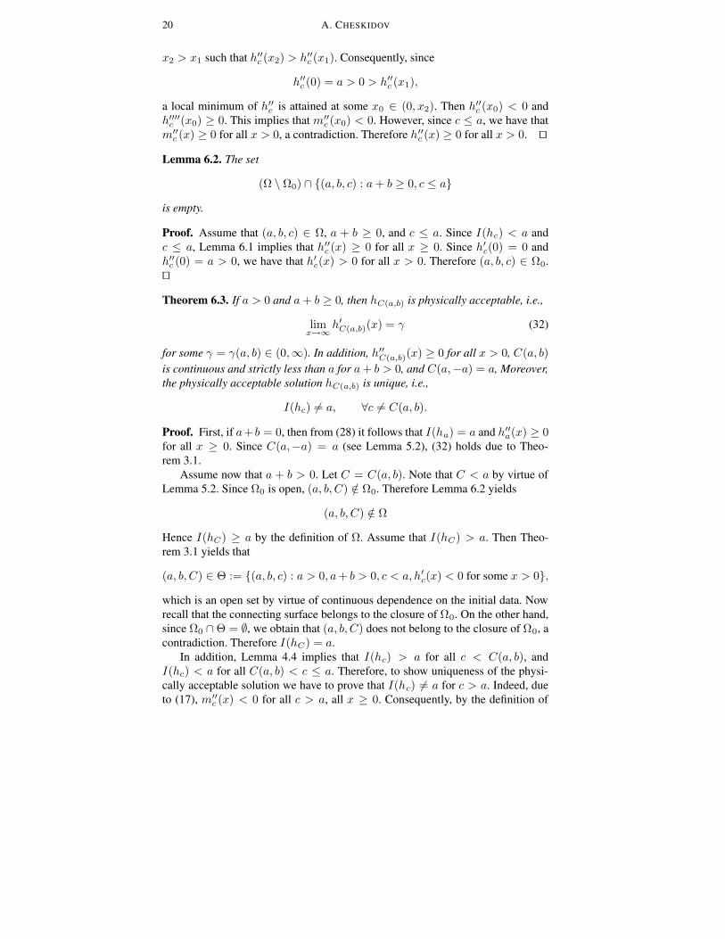
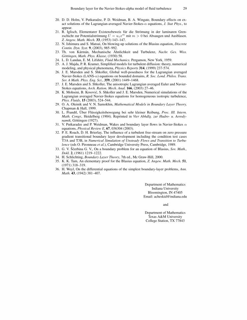
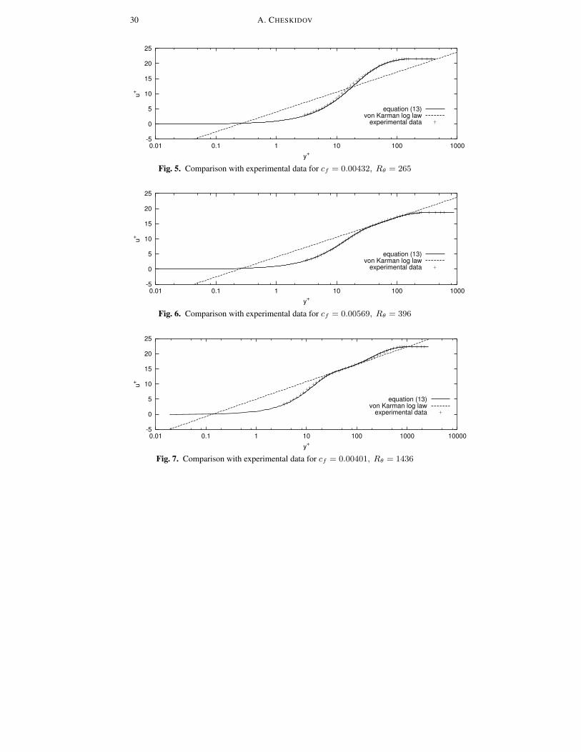
Here ξ0 is the middle inflection point of h′(ξ) in logarithmic coordinates.Varying Rθ and cf , we obtain a family of the velocity profiles u+

Rθ,cf. This

family was compared with experimental data of the Rolls-Royce applied sciencelaboratory, ERCOFTAC t3b test case [32] (see Fig. 5–7). Comparison shows thatthe case a+ b > 0 corresponds to the laminar boundary layer, whereas a+ b < 0corresponds to the transitional and turbulent boundary layers.

9. Appendix. Blasius equation

The Blasius equation is written as

h′′′ +1

2hh′′ = 0. (45)

The physical boundary conditions are h(0) = h′(0) = 0, and h′(ξ) → 1 asξ →∞.

Theorem 9.1. There exists a unique solution h(x) to (45) satisfying the physicalboundary conditions. In addition, the Blasius profile h′(x) has one inflection pointin logarithmic coordinates.

Proof. The existence and uniqueness is a classical result and can be found, e.g.,in [18]. Nevertheless, we present a short proof here for completeness.

For a given a ∈ R, let ha(x) be the solution of (45) with ha(0) = h′a(0) = 0,h′′a(x) = a. Then

h′′a(x) = ae−12

R x0ha(y) dy. (46)

Obviously, if a ≤ 0, then ha(x) does not satisfy the physical boundary conditions.If a > 0, then (46) implies that h′′a(x) > 0 for all x ≥ 0 and, consequently,∫ x

0ha(y) dy increases faster than a linear function. Therefore, using (46) again,

we conclude that h′a(x)→ γ(a) for some γ(a) > 0. Finally, since

ha(x) =√ah1(√ax),

we have that γ(a) = aγ(1). Hence, there exists a unique solution h(x) to (45) sat-isfying the physical boundary conditions. In fact, h(x) = ha(x) for a = 1/γ(1).For this h(x), the function h′(x), x ∈ [0,∞), will be be called a Blasius profile.

To study the Blasius profile in logarithmic coordinates, let z = lnx andF (z) =h′(ez). Then (45) yields

F ′′(z) = aez−12

R ez0

h(y) dy

(1− 1

2ezh(ez)

).

Since h(0) = 0 and h(x) is increasing, F ′′(z) changes sign once, i.e. the Blasiusprofile has one inflection point in logarithmic coordinates. ut

28 A. CHESKIDOV

Acknowledgements. This subject was suggested by my thesis advisor, Ciprian Foias, andthe work was completed while I was a graduate student at Indiana University. I am deeplygrateful for his help and support. In addition, I would like to thank D. D. Holm, M. S. Jolly,E. Olson, C. M. Pearcy, R. Temam, and E. S. Titi for stimulating discussions and comments.I would also like to thank P. Holmes for careful reading and detailed comments that led tosignificant improvement of the paper. This work was supported in part by NSF grants DMS-0074334, and DMS-0074460.

References

1. G. I. Barenblatt, A. J. Chorin, V. M. Prostokishin, Self-similar intermediate structuresin turbulent boundary layers at large Reynolds numbers, J. Fluid Mech. 410, (2000)263–283.

2. Z. Belhachmi, B. Brighi, K. Taous, On the concave solutions of the Blasius equation,Acta Math. Univ. Comenian. (N.S.) 69, (2000) 199–214.

3. H. Blasius, Grenzschichten in Flussigkeiten mit Kleiner Reibung, Z. Math. u. Phys. 56,(1908) 1–37.

4. T. Cebeci, J. Cousteix, Modeling and Computation of Boundary-Layer Flows. HorizonsPublishing Inc., Long Beach, CA, 1999.

5. S. Chen, C. Foias, D. D. Holm, E. Olson, E. S. Titi, S. Wynne, The Camassa-Holmequations as a closure model for turbulent channel and pipe flow, Phys. Rev. Lett. 81,(1998) 5338–5341.

6. S. Chen, C. Foias, D. D. Holm, E. Olson, E. S. Titi, S. Wynne, A connection betweenthe Camassa-Holm equations and turbulent flows in pipes and channels, Phys. Fluids,11 (1999) 2343–2353.

7. S. Chen, C. Foias, D. D. Holm, E. Olson, E. S. Titi, S. Wynne, The Camassa-Holmequations and turbulence, Physica D 133, (1999) 49–65.

8. A. Cheskidov, Turbulent boundary layer equations, C. R. Acad. Sci. Paris, Ser. I 334,(2002) 423–427.

9. A. Cheskidov, D. D. Holm, E. Olson, and E. S. Titi, On a Leray-αModel of Turbulence,preprint.

10. D. Coles, The law of the wake in the turbulent boundary layer, J. Fluid Mech. 1, (1956)191–226.

11. P. Constantin, Filtered viscous fluid equations, Computer and Mathematics with Appli-cations, to appear.

12. W. A. Coppel, On a differential equation of boundary layer theory, Phil. Trans. Roy.Soc. London Ser. A 253, (1960) 101–136.

13. J. A. Domaradzki, D. D. Holm, Navier Stokes-alpha model: LES equations with non-linear dispersion, Special LES volume of ERCOFTAC Bulletin, Modern SimulationsStrategies for turbulent flow. B. J. Geurts, editor, Edwards Publishing.

14. H. H. Fernholtz, P. J. Finley, The incompressible zero-pressure-gradient boundarylayer: an assessment of the data. Prog. Aerospace Sci. 32, (1996) 245–311.

15. C. Foias, D. D. Holm, E. S. Titi, The Navier-Stokes-alpha model of fluid turbulence,Physica D 152, (2001) 505–519.

16. C. Foias, D. D. Holm, and E. S. Titi, The three dimensional viscous Camassa–Holmequations, and their relation to the Navier–Stokes equations and turbulence theory,Journal of Dynamics and Differential Equations 14, (2002) 1–35.

17. S. Furuya, Note on a boundary value problem, Comment. Math. Univ. St Paul 1, (1953)81–83.

18. P. Hartman, Ordinary Differential Equations. John Wiley & Sons, Inc., New York,London, Sidney, 1964.

19. D. D. Holm, J. E. Marsden, T. S. Ratiu, Euler-Poincare Models of Ideal Fluids withNonlinear Dispersion, Phys. Rev. Lett. 80, (1998) 4173–4176.


20. D. D. Holm, V. Putkaradze, P. D. Weidman, B. A. Wingate, Boundary effects on ex-act solutions of the Lagrangian-averaged Navier-Stokes-α equations, J. Stat Phys., toappear.

21. R. Iglisch, Elementarer Existenzbeweis fur die Stromung in der laminaren Gren-zschicht zur Potentialstromung U = u1x

m mit m > 0 bei Absaugen und Ausblasen.Z. Angew. Math. Mech. 33, (1953) 143–147.

22. N. Ishimura and S. Matsui, On blowing-up solutions of the Blasius equation, DiscreteContin. Dyn. Syst. 9, (2003), 985–992.

23. Th. von Karman, Mechanische Ahnlichkeit und Turbulenz, Nachr. Ges. Wiss.Gottingen, Math. Phys. Klasse, (1930) 58.

24. L. D. Landau, E. M. Lifshitz, Fluid Mechanics. Pergamon, New York, 1959.25. A. J. Majda, P. R. Kramer, Simplified models for turbulent diffusion: theory, numerical

modeling, and physical phenomena, Physics Reports 314, (1999) 237-574.26. J. E. Marsden and S. Shkoller, Global well-posedness for the Lagrangian averaged

Navier-Stokes (LANS-α) equations on bounded domains, R. Soc. Lond. Philos. Trans.Ser. A Math. Phys. Eng. Sci., 359, (2001) 1449–1468.

27. J. E. Marsden and S. Shkoller, The anisotropic Lagrangian averaged Euler and Navier-Stokes equations, Arch. Ration. Mech. Anal. 166, (2003) 27–46.

28. K. Mohseni, B. Kosovic, S. Shkoller and J. E. Marsden, Numerical simulations of theLagrangian averaged Navier-Stokes equations for homogeneous isotropic turbulence,Phys. Fluids, 15 (2003), 524–544.

29. O. A. Oleinik and V. N. Samokhin, Mathematical Models in Boundary Layer Theory,Chapman & Hall, 1999.

30. L. Prandtl, Uber Flussigkeitsbewegung bei sehr kleiner Reibung, Proc. III. Intern.Math. Congr., Heidelberg (1904). Reprinted in Vier Abhdlg. zur Hudro- u. Aerody-namik, Gottingen (1927).

31. V. Putkaradze and P. Weidman, Wakes and boundary layer flows in Navier-Stokes αequations, Physical Review E, 67, 036304 (2003).

32. P. E. Roach, D. H. Brierlay, The influence of a turbulent free-stream on zero pressuregradient transitional boundary layer development including the condition test casesT3A and T3B, in Numerical Simulation of Unsteady Flows and Transition to Turbu-lence (eds O. Pironneau et al.), Cambridge University Press, Cambridge, 1989.

33. G. V. Scerbina G. V., On a boundary problem for an equation of Blasius, Sov. Math.,Dokl. 2, (1961) 1219–1222.

34. H. Schlichting, Boundary Layer Theory, 7th ed., Mc Graw-Hill, 2000.35. K. K. Tam, An elementary proof for the Blasius equation, Z. Angew. Math. Mech. 51,

(1971) 318–319.36. H. Weyl, On the differential equations of the simplest boundary-layer problems, Ann.

Math. 43, (1942) 381–407.

Department of MathematicsIndiana University

Bloomington, IN 47405Email: [email protected]

and

Department of MathematicsTexas A&M University

College Station, TX 77843

30 A. CHESKIDOV

-5

0

5

10

15

20

25

0.01 0.1 1 10 100 1000u+

y+

equation (13)von Karman log law

experimental data

Fig. 5. Comparison with experimental data for cf = 0.00432, Rθ = 265

-5

0

5

10

15

20

25

0.01 0.1 1 10 100 1000

u+

y+


experimental data


-5

0

5

10

15

20

25

0.01 0.1 1 10 100 1000 10000

u+

y+


experimental data


Documents

Boundary layer for the Navier-Stokes-alpha model of …homepages.math.uic.edu/~acheskid/papers/ch.pdfBoundary layer for the Navier-Stokes-alpha model of uid turbulence? A. CHESKIDOV