Embed Size (px)
Citation preview
2-1
ME 306 Fluid Mechanics II
Part 2
Viscous Flow over Immersed Bodies
These presentations are prepared by
Dr. Cüneyt Sert
Department of Mechanical Engineering
Middle East Technical University
Ankara, Turkey
Please ask for permission before using them. You are NOT allowed to modify them.
2-2
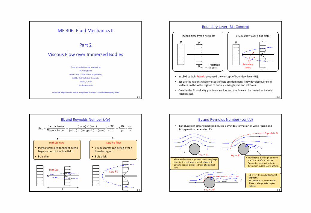
Boundary Layer (BL) Concept
Viscous flow over a flat plate
• In 1904 Ludwig Prandtl proposed the concept of boundary layer (BL).
• BLs are the regions where viscous effects are dominant. They develop over solidsurfaces, in the wake regions of bodies, mixing layers and jet flows.
• Outside the BLs velocity gradients are low and the flow can be treated as inviscid (frictionless).
𝑈𝑈
𝑈
Boundary layers
Inviscid flow over a flat plate
𝑈 𝑈
𝑈Freestream velocity
2-3
BL and Reynolds Number (𝑅𝑒)
𝑅𝑒𝐿 =Inertia forces
Viscous forces=
(mass) × (acc. )
(visc. ) × (vel. grad. ) × (area)
𝜌𝐿2𝑈2
𝜇𝑈𝐿=
𝜌𝑈𝐿
𝜇=
𝑈𝐿
𝜈
Low 𝑅𝑒
High 𝑅𝑒 flow
• Inertia forces are dominant over a large portion of the flow field.
• BL is thin.
Low 𝑅𝑒 flow
• Viscous forces can be felt over a broader region.
• BL is thick.
High 𝑅𝑒
𝐿2-4
BL and Reynolds Number (cont’d)
• For blunt (not streamlined) bodies, like a cylinder, formation of wake region and BL separation depend on 𝑅𝑒.
𝑅𝑒𝐷 = 0.1
• Viscous effects are important over a very large domain. It is not proper to talk about a BL.
• Streamlines are similar to those of potential flow.
• Fluid inertia is too high to follow the contour of the cylinder.
• Separation occurs at point A. Circulation bubble forms behind.
• BL is very thin and attached at the front.
• BL separates at the rear side.• There is a large wake region
behind.
Edge of the BL
𝑅𝑒𝐷 = 50
A
Wake
𝑅𝑒𝐷 = 105
A
2-5
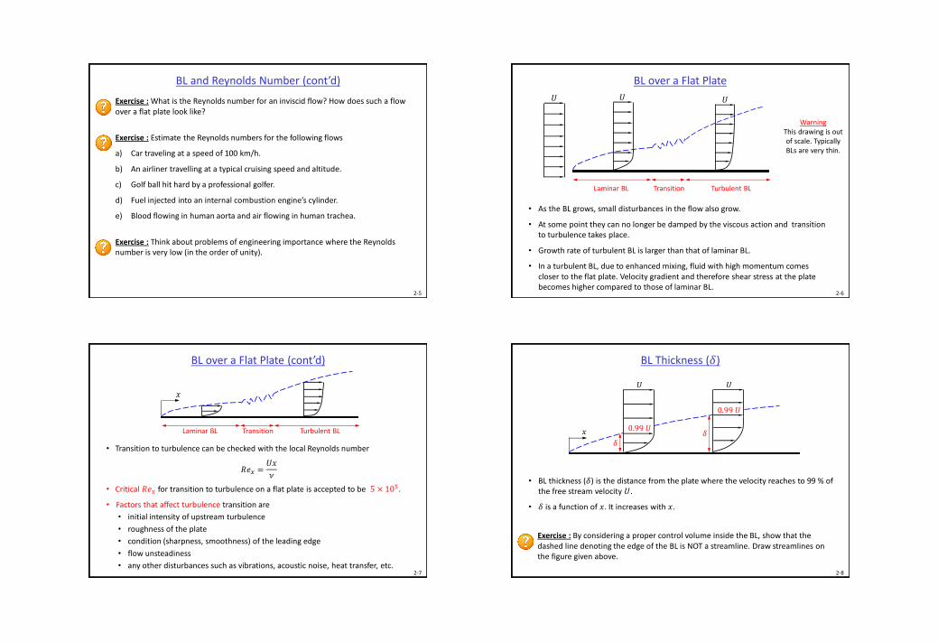
BL and Reynolds Number (cont’d)
Exercise : What is the Reynolds number for an inviscid flow? How does such a flow over a flat plate look like?
Exercise : Estimate the Reynolds numbers for the following flows
a) Car traveling at a speed of 100 km/h.
b) An airliner travelling at a typical cruising speed and altitude.
c) Golf ball hit hard by a professional golfer.
d) Fuel injected into an internal combustion engine’s cylinder.
e) Blood flowing in human aorta and air flowing in human trachea.
Exercise : Think about problems of engineering importance where the Reynolds number is very low (in the order of unity).
2-6
BL over a Flat Plate
• As the BL grows, small disturbances in the flow also grow.
• At some point they can no longer be damped by the viscous action and transition to turbulence takes place.
• Growth rate of turbulent BL is larger than that of laminar BL.
• In a turbulent BL, due to enhanced mixing, fluid with high momentum comes closer to the flat plate. Velocity gradient and therefore shear stress at the plate becomes higher compared to those of laminar BL.
WarningThis drawing is out of scale. Typically BLs are very thin.
𝑈 𝑈
Laminar BL
𝑈
Turbulent BLTransition
2-7
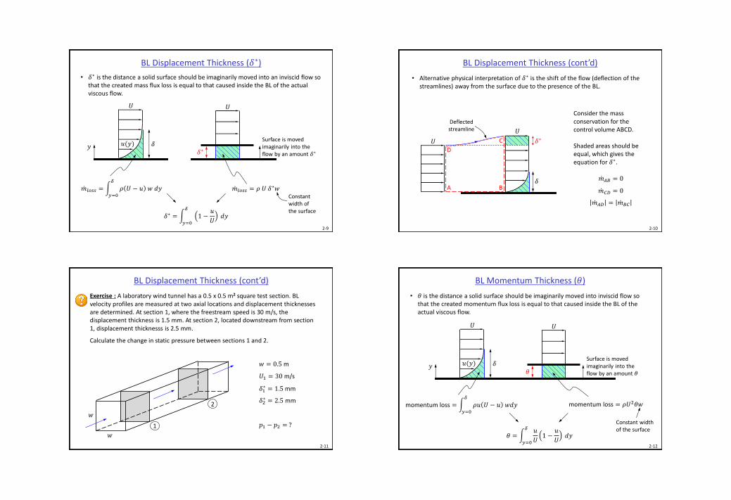
BL over a Flat Plate (cont’d)
• Transition to turbulence can be checked with the local Reynolds number
𝑅𝑒𝑥 =𝑈𝑥
𝜈
• Critical 𝑅𝑒𝑥 for transition to turbulence on a flat plate is accepted to be 5 × 10⁵.
• Factors that affect turbulence transition are
• initial intensity of upstream turbulence
• roughness of the plate
• condition (sharpness, smoothness) of the leading edge
• flow unsteadiness
• any other disturbances such as vibrations, acoustic noise, heat transfer, etc.
Laminar BL Turbulent BLTransition
𝑥
2-8
BL Thickness (𝛿)
• BL thickness (𝛿) is the distance from the plate where the velocity reaches to 99 % of the free stream velocity 𝑈.
• 𝛿 is a function of 𝑥. It increases with 𝑥.
Exercise : By considering a proper control volume inside the BL, show that the dashed line denoting the edge of the BL is NOT a streamline. Draw streamlines on the figure given above.
𝑈
𝛿
𝑥
𝑈
𝛿0.99 𝑈
0.99 𝑈
2-9
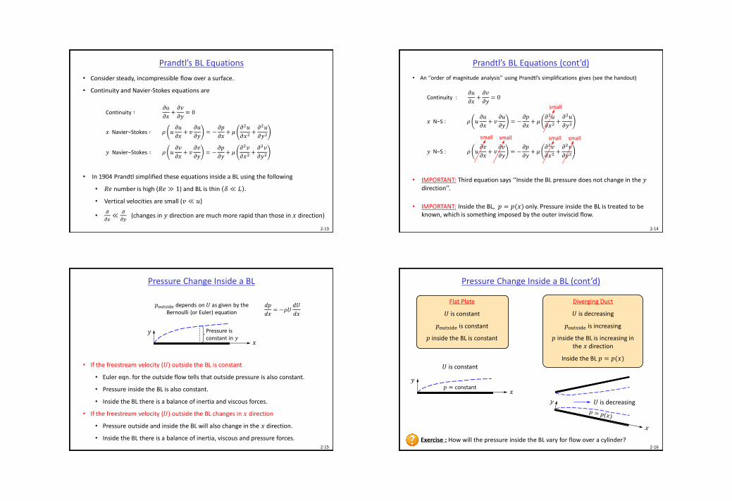
BL Displacement Thickness (𝛿∗)
• 𝛿∗ is the distance a solid surface should be imaginarily moved into an inviscid flow so that the created mass flux loss is equal to that caused inside the BL of the actual viscous flow.
𝛿∗ = 𝑦=0
𝛿
1 −𝑢
𝑈𝑑𝑦
𝑈
𝛿𝑦 𝑢(𝑦)
𝑚𝑙𝑜𝑠𝑠 = 𝑦=0
𝛿
𝜌 𝑈 − 𝑢 𝑤 𝑑𝑦
Surface is moved imaginarily into the flow by an amount 𝛿∗𝛿∗
𝑈
Constant width of the surface
𝑚𝑙𝑜𝑠𝑠 = 𝜌 𝑈 𝛿∗𝑤
2-10
BL Displacement Thickness (cont’d)
• Alternative physical interpretation of 𝛿∗ is the shift of the flow (deflection of thestreamlines) away from the surface due to the presence of the BL.
Consider the mass conservation for the control volume ABCD.
Shaded areas should be equal, which gives the equation for 𝛿∗.
𝑚𝐴𝐵 = 0
𝑚𝐶𝐷 = 0
𝑚𝐴𝐷 = 𝑚𝐵𝐶
𝑈
𝛿
𝑈
Deflectedstreamline
𝛿∗
A B
D
C
2-11
BL Displacement Thickness (cont’d)
Exercise : A laboratory wind tunnel has a 0.5 x 0.5 m2 square test section. BLvelocity profiles are measured at two axial locations and displacement thicknesses are determined. At section 1, where the freestream speed is 30 m/s, the displacement thickness is 1.5 mm. At section 2, located downstream from section 1, displacement thicknesss is 2.5 mm.
Calculate the change in static pressure between sections 1 and 2.
𝑤 = 0.5 m
𝑈1 = 30 m/s
𝛿1∗ = 1.5 mm
𝛿2∗ = 2.5 mm
𝑝1 − 𝑝2 = ?1
2
𝑤
𝑤
2-12
BL Momentum Thickness (𝜃)
• 𝜃 is the distance a solid surface should be imaginarily moved into inviscid flow so that the created momentum flux loss is equal to that caused inside the BL of the actual viscous flow.
𝜃 = 𝑦=0
𝛿 𝑢
𝑈1 −
𝑢
𝑈𝑑𝑦
Surface is moved imaginarily into the flow by an amount 𝜃
𝑈
𝜃
𝑈
𝛿𝑦 𝑢(𝑦)
momentum loss = 𝜌𝑈2𝜃𝑤momentum loss = 𝑦=0
𝛿
𝜌𝑢 𝑈 − 𝑢 𝑤𝑑𝑦
Constant width of the surface
• Consider steady, incompressible flow over a surface.
• Continuity and Navier-Stokes equations are
Continuity ∶𝜕𝑢
𝜕𝑥+
𝜕𝑣
𝜕𝑦= 0
𝑥 Navier−Stokes ∶ 𝜌 𝑢𝜕𝑢
𝜕𝑥+ 𝑣
𝜕𝑢
𝜕𝑦= −
𝜕𝑝
𝜕𝑥+ 𝜇
𝜕2𝑢
𝜕𝑥2+
𝜕2𝑢
𝜕𝑦2
𝑦 Navier−Stokes ∶ 𝜌 𝑢𝜕𝑣
𝜕𝑥+ 𝑣
𝜕𝑣
𝜕𝑦= −
𝜕𝑝
𝜕𝑦+ 𝜇
𝜕2𝑣
𝜕𝑥2+
𝜕2𝑣
𝜕𝑦2
• In 1904 Prandtl simplified these equations inside a BL using the following
• 𝑅𝑒 number is high (𝑅𝑒 ≫ 1) and BL is thin 𝛿 ≪ 𝐿 .
• Vertical velocities are small (𝑣 ≪ 𝑢)
•𝜕
𝜕𝑥≪
𝜕
𝜕𝑦(changes in 𝑦 direction are much more rapid than those in 𝑥 direction)
2-13
Prandtl’s BL Equations Prandtl’s BL Equations (cont’d)
• An ‘‘order of magnitude analysis’’ using Prandtl’s simplifications gives (see the handout)
Continuity :𝜕𝑢
𝜕𝑥+
𝜕𝑣
𝜕𝑦= 0
𝑥 N−S : 𝜌 𝑢𝜕𝑢
𝜕𝑥+ 𝑣
𝜕𝑢
𝜕𝑦= −
𝜕𝑝
𝜕𝑥+ 𝜇
𝜕2𝑢
𝜕𝑥2+
𝜕2𝑢
𝜕𝑦2
𝑦 N−S : 𝜌 𝑢𝜕𝑣
𝜕𝑥+ 𝑣
𝜕𝑣
𝜕𝑦= −
𝜕𝑝
𝜕𝑦+ 𝜇
𝜕2𝑣
𝜕𝑥2+
𝜕2𝑣
𝜕𝑦2
• IMPORTANT: Third equation says ‘‘Inside the BL pressure does not change in the 𝑦direction’’.
• IMPORTANT: Inside the BL, 𝑝 = 𝑝(𝑥) only. Pressure inside the BL is treated to be known, which is something imposed by the outer inviscid flow.
small
small small small small
2-14
2-15
Pressure Change Inside a BL
• If the freestream velocity (𝑈) outside the BL is constant
• Euler eqn. for the outside flow tells that outside pressure is also constant.
• Pressure inside the BL is also constant.
• Inside the BL there is a balance of inertia and viscous forces.
• If the freestream velocity (𝑈) outside the BL changes in 𝑥 direction
• Pressure outside and inside the BL will also change in the 𝑥 direction.
• Inside the BL there is a balance of inertia, viscous and pressure forces.
𝑥
𝑦 Pressure is constant in 𝑦
𝑝outside depends on 𝑈 as given by theBernoulli (or Euler) equation
𝑑𝑝
𝑑𝑥= −𝜌𝑈
𝑑𝑈
𝑑𝑥
2-16
Pressure Change Inside a BL (cont’d)
Flat Plate
𝑈 is constant
𝑝outside is constant
𝑝 inside the BL is constant
Diverging Duct
𝑈 is decreasing
𝑝outside is increasing
𝑝 inside the BL is increasing in the 𝑥 direction
Inside the BL 𝑝 = 𝑝(𝑥)
𝑥
𝑦𝑝 = constant
𝑈 is constant
Exercise : How will the pressure inside the BL vary for flow over a cylinder?
𝑈 is decreasing
2-17
Pressure Change Inside a BL (cont’d)
• Static holes are used to measure pressure distribution on a wall.
• Since 𝑝 does not change in the 𝑦 direction inside the BL, the measured pressures are equal to the ones at the edge of the BL.
• Therefore an inviscid Euler solution or even a potential flow solution for the flow outsidethe BL may predict correct pressuredistribution over the surface.
• This is the reason why inviscid flow solutions over streamlined bodies such as airfoils can predict the lift force accurately.
• It is not the case for airfoils at high angle of attack or for blunt bodies due to flow separation. BL theory is not valid after the separation point.
-6
-4
-3
-2
-1
0
-10.0 0.2 0.4 0.6 0.8 1.0
Potential FlowExperiment
𝐶𝑝
Pressure distribution on an airfoil
𝑈∞
Çengel’s book
𝑥𝛿
𝑦
𝑝1
𝑝2
𝑝1 𝑝2
BL
Presssure taps
2-18
Blasius’ Exact Solution of BL over a Flat Plate
• In 1908 Blasius, a student of Prandtl, obtained the analytical solution of the following BL equations for laminar flow over a flat plate with zero pressure gradient.
𝜕𝑢
𝜕𝑥+
𝜕𝑣
𝜕𝑦= 0
𝜌 𝑢𝜕𝑢
𝜕𝑥+ 𝑣
𝜕𝑢
𝜕𝑦= 𝜇
𝜕2𝑢
𝜕𝑦2
• He used the following boundary conditions
• At 𝑦 = 0 : 𝑢 = 0 & 𝑣 = 0 (No-slip)
• As 𝑦 → ∞ : 𝑢 → 𝑈 (Asymptotic approach to free stream velocity)
• Blasius’ solution is valid for laminar flow over a flat plate with no pressure gradient.
• The solution uses streamfunction and a similarity transformation. You are NOT responsible for its details.
𝑑𝑝/𝑑𝑥 is zero for flat plate
2-19
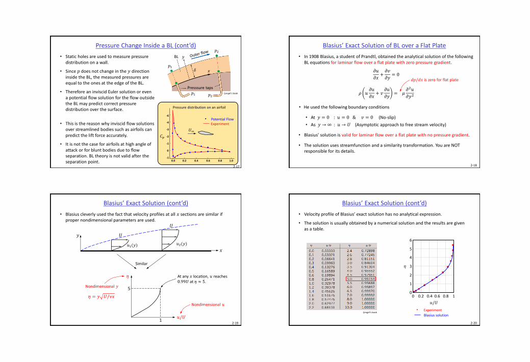
Blasius’ Exact Solution (cont’d)
• Blasius cleverly used the fact that velocity profiles at all 𝑥 sections are similar if proper nondimensional parameters are used.
𝑢/𝑈
𝜂
5
1
Nondimensional 𝑢
Nondimensional 𝑦
𝜂 = 𝑦 𝑈/𝜈𝑥
At any 𝑥 location, 𝑢 reaches 0.99𝑈 at 𝜂 ≈ 5.
Similar
𝑥
𝑈
𝑈
𝑢1(𝑦) 𝑢2(𝑦)
𝑦
2-20
Blasius’ Exact Solution (cont’d)
• Velocity profile of Blasius’ exact solution has no analytical expression.
• The solution is usually obtained by a numerical solution and the results are given as a table.
Experiment
Blasius solution
𝑢/𝑈
0 0.2 0.4 0.6 0.8 1
𝜂
6
5
4
3
2
1
0
Çengel’s book
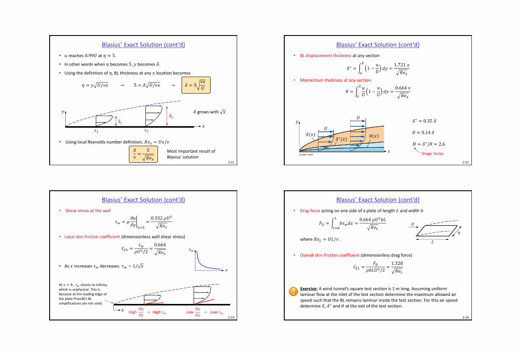
• 𝑢 reaches 0.99𝑈 at 𝜂 ≈ 5.
• In other words when 𝜂 becomes 5, 𝑦 becomes 𝛿.
• Using the definition of 𝜂, BL thickness at any 𝑥 location becomes
𝜂 = 𝑦 𝑈/𝜈𝑥 → 5 = 𝛿 𝑈/𝜈𝑥 → 𝛿 = 5𝜈𝑥
𝑈
• Using local Reynolds number definition, 𝑅𝑒𝑥 = 𝑈𝑥/𝜈
𝛿
𝑥=
5
𝑅𝑒𝑥2-21
Blasius’ Exact Solution (cont’d)
Most important result of Blasius’ solution
𝛿 grows with 𝑥
𝛿1
𝛿2
𝑥
𝑦
𝑥1 𝑥2
2-22
Blasius’ Exact Solution (cont’d)
• BL displacement thickness at any section
𝛿∗ = 0
𝛿
1 −𝑢
𝑈𝑑𝑦 =
1.721 𝑥
𝑅𝑒𝑥
• Momentum thickness at any section
𝜃 = 0
𝛿 𝑢
𝑈1 −
𝑢
𝑈𝑑𝑦 =
0.664 𝑥
𝑅𝑒𝑥
𝛿∗ ≈ 0.35 𝛿
𝜃 ≈ 0.14 𝛿
𝐻 = 𝛿∗/𝜃 ≈ 2.6
Shape factorÇengel’s book
𝛿∗(𝑥)𝜃(𝑥)𝛿(𝑥)
𝑥
𝑦
𝑈
𝑈
2-23
Blasius’ Exact Solution (cont’d)
• Shear stress at the wall
𝜏𝑤 = 𝜇 𝜕𝑢
𝜕𝑦𝑦=0
=0.332 𝜌𝑈2
𝑅𝑒𝑥
• Local skin friction coefficient (dimensionless wall shear stress)
𝐶𝑓𝑥 =𝜏𝑤
𝜌𝑈2/2=
0.664
𝑅𝑒𝑥
• As 𝑥 increases 𝜏𝑤 decreases. 𝜏𝑤 ~ 1/ 𝑥
𝑥 High𝜕𝑢
𝜕𝑦→ High 𝜏𝑤 Low
𝜕𝑢
𝜕𝑦→ Low 𝜏𝑤
At 𝑥 = 0, 𝜏𝑤 shoots to infinity, which is unphysical. This is because at the leading edge of the plate Prandtl’s BL simplifications are not valid.
𝑥
𝜏𝑤
2-24
Blasius’ Exact Solution (cont’d)
• Drag force acting on one side of a plate of length 𝐿 and width 𝑏
𝐹𝐷 = 𝑥=0
𝐿
𝑏𝜏𝑤𝑑𝑥 =0.664 𝜌𝑈2𝑏𝐿
𝑅𝑒𝐿
where 𝑅𝑒𝐿 = 𝑈𝐿/𝜈 .
• Overall skin friction coefficient (dimensionless drag force)
𝐶𝑓𝐿 =𝐹𝐷
𝜌𝑏𝐿𝑈2/2=
1.328
𝑅𝑒𝐿
Exercise: A wind tunnel’s square test section is 1 m long. Assuming uniform laminar flow at the inlet of the test section determine the maximum allowed air speed such that the BL remains laminar inside the test section. For this air speed determine 𝛿, 𝛿∗ and 𝜃 at the exit of the test section.
𝐿
𝑏
𝑈
2-25
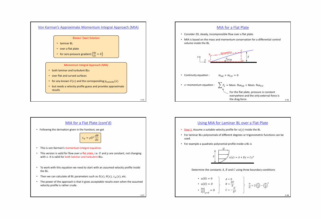
Von Karman’s Approximate Momentum Integral Approach (MIA)
Momentum Integral Approach (MIA)
• both laminar and turbulent BLs
• over flat and curved surfaces
• for any known 𝑈(𝑥) and the corresponding 𝑝outside(𝑥)
• but needs a velocity profile guess and provides approximate results
Blasius’ Exact Solution
• laminar BL
• over a flat plate
• for zero pressure gradient 𝑑𝑝
𝑑𝑥= 0
2-26
MIA for a Flat Plate
• Consider 2D, steady, incompressible flow over a flat plate.
• MIA is based on the mass and momentum conservation for a differential control volume inside the BL.
• Continuity equation :
• 𝑥–momentum equation : 𝐹𝑥 = Mom. flux𝐴𝐵 + Mom. flux𝐶𝐷
𝑚𝐴𝐵 + 𝑚𝐶𝐷 = 0
For the flat plate, pressure is constant everywhere and the only external force is the drag force.
𝑥𝑦
A D
C
B𝛿
𝐹𝑑𝑟𝑎𝑔
• Following the derivation given in the handout, we get
𝜏𝑤 = 𝜌𝑈2𝑑𝜃
𝑑𝑥
• This is von Karman’s momentum integral equation.
• This version is valid for flow over a flat plate, i.e. 𝑈 and 𝑝 are constant, not changing with 𝑥. It is valid for both laminar and turbulent BLs.
• To work with this equation we need to start with an assumed velocity profile inside the BL.
• Then we can calculate all BL parameters such as 𝛿(𝑥), 𝜃(𝑥), 𝜏𝑤(𝑥), etc.
• The power of the approach is that it gives acceptable results even when the assumed velocity profile is rather crude.
2-27
MIA for a Flat Plate (cont’d)
2-28
Using MIA for Laminar BL over a Flat Plate
• Step 1. Assume a suitable velocity profile for 𝑢(𝑦) inside the BL
• For laminar BLs polynomials of different degrees or trigonometric functions can be used.
• For example a quadratic polynomial profile inside a BL is
𝑢 𝑦 = 𝐴 + 𝐵𝑦 + 𝐶𝑦2𝛿
𝑈
Determine the constants 𝐴, 𝐵 and 𝐶 using three boundary conditions
• 𝑢 0 = 0
• 𝑢 𝛿 = 𝑈
• 𝜕𝑢
𝜕𝑦 𝑦=𝛿= 0
𝑢
𝑈= 2
𝑦
𝛿−
𝑦
𝛿
2
𝐴 = 0
𝐵 =2𝑈
𝛿
𝐶 = −𝑈
𝛿2
2-29
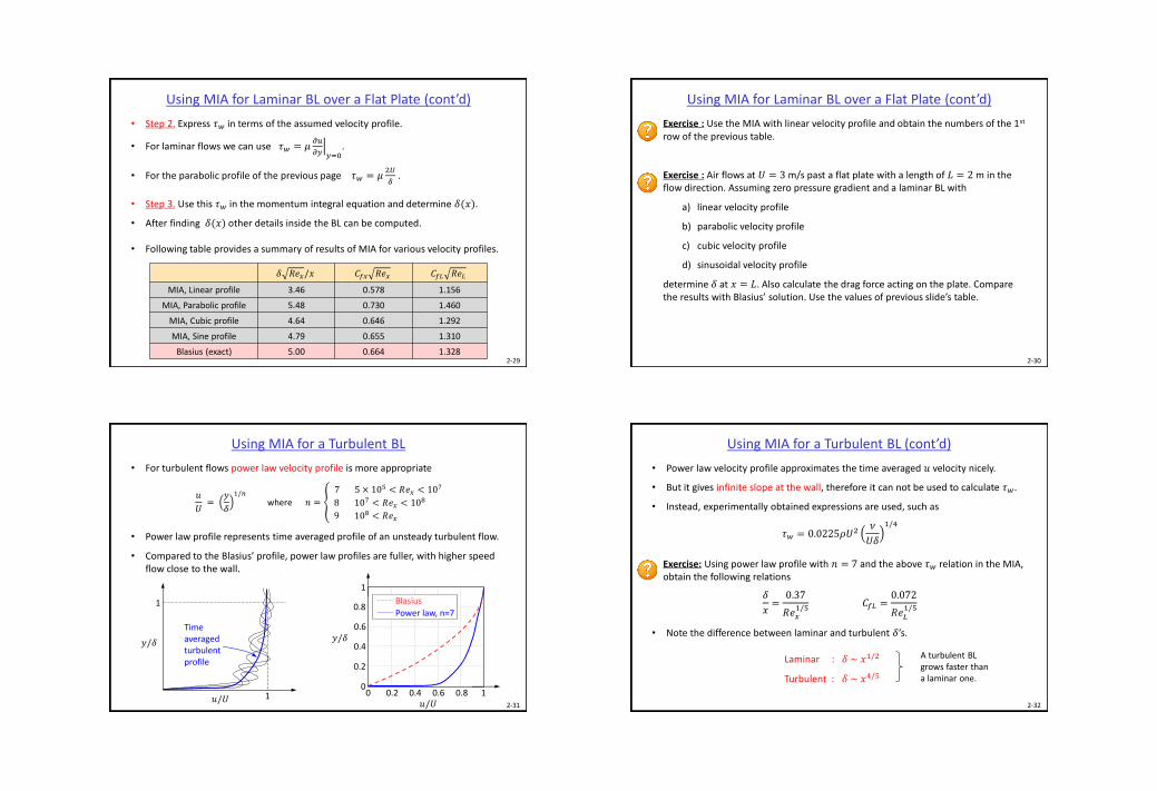
Using MIA for Laminar BL over a Flat Plate (cont’d)
• Step 2. Express 𝜏𝑤 in terms of the assumed velocity profile.
• For laminar flows we can use 𝜏𝑤 = 𝜇 𝜕𝑢
𝜕𝑦 𝑦=0.
• For the parabolic profile of the previous page 𝜏𝑤 = 𝜇2𝑈
𝛿.
• Step 3. Use this 𝜏𝑤 in the momentum integral equation and determine 𝛿(𝑥).
• After finding 𝛿(𝑥) other details inside the BL can be computed.
• Following table provides a summary of results of MIA for various velocity profiles.
𝛿 𝑅𝑒𝑥/𝑥 𝐶𝑓𝑥 𝑅𝑒𝑥 𝐶𝑓𝐿 𝑅𝑒𝐿
MIA, Linear profile 3.46 0.578 1.156
MIA, Parabolic profile 5.48 0.730 1.460
MIA, Cubic profile 4.64 0.646 1.292
MIA, Sine profile 4.79 0.655 1.310
Blasius (exact) 5.00 0.664 1.3282-30
Exercise : Use the MIA with linear velocity profile and obtain the numbers of the 1st
row of the previous table.
Exercise : Air flows at 𝑈 = 3 m/s past a flat plate with a length of 𝐿 = 2 m in the flow direction. Assuming zero pressure gradient and a laminar BL with
a) linear velocity profile
b) parabolic velocity profile
c) cubic velocity profile
d) sinusoidal velocity profile
determine 𝛿 at 𝑥 = 𝐿. Also calculate the drag force acting on the plate. Compare the results with Blasius’ solution. Use the values of previous slide’s table.
Using MIA for Laminar BL over a Flat Plate (cont’d)
2-31
Using MIA for a Turbulent BL
• For turbulent flows power law velocity profile is more appropriate
𝑢
𝑈=
𝑦
𝛿
1/𝑛
where 𝑛 =
7 5 × 10⁵ < 𝑅𝑒𝑥 < 107
8 107 < 𝑅𝑒𝑥 < 108
9 108 < 𝑅𝑒𝑥
• Power law profile represents time averaged profile of an unsteady turbulent flow.
• Compared to the Blasius’ profile, power law profiles are fuller, with higher speed flow close to the wall.
𝑦/𝛿
𝑢/𝑈
1
1
Time averaged turbulent profile
1
0 0.2 0.4 0.6 0.8 1
0.8
0.6
0.4
0.2
0
Blasius
Power law, n=7
𝑦/𝛿
𝑢/𝑈 2-32
Using MIA for a Turbulent BL (cont’d)
• Power law velocity profile approximates the time averaged 𝑢 velocity nicely.
• But it gives infinite slope at the wall, therefore it can not be used to calculate 𝜏𝑤.
• Instead, experimentally obtained expressions are used, such as
𝜏𝑤 = 0.0225𝜌𝑈2𝜈
𝑈𝛿
1/4
Exercise: Using power law profile with 𝑛 = 7 and the above 𝜏𝑤 relation in the MIA, obtain the following relations
𝛿
𝑥=
0.37
𝑅𝑒𝑥1/5
𝐶𝑓𝐿 =0.072
𝑅𝑒𝐿1/5
• Note the difference between laminar and turbulent 𝛿’s.
Laminar : 𝛿 ~ 𝑥1/2
Turbulent : 𝛿 ~ 𝑥4/5
A turbulent BL grows faster than a laminar one.

2-33
Drag Force Calculation using Integral Formulation (similar to MIA)
Exercise: (Fox’s book) A developing boundary layer of standard air on a flat plate is shown below. The free stream flow outside the boundary layer is undisturbed with 𝑈 = 50 m/s. The plate is 3 m wide perpendicular to the diagram. Measurements at section BC revealed that the velocity profile is close to power law profile with 𝑛 = 7 and boundary layer thickness is 𝛿 = 19 mm. Calculate
a) the mass flow rates across surfaces AD, AB and BC.
b) the x-momentum flow rates across surfaces AD, AB and BC.
c) the drag force exerted on the flat plate between D and C.
𝛿
𝑈
CV
𝑥
𝑦
A B
CD
2-34
Pressure Gradient Inside a Boundary Layer
𝑑𝑈
𝑑𝑥> 0 &
𝑑𝑝
𝑑𝑥< 0
Pressure drops in flow direction (Favorable pressure gradient)
𝑑𝑈
𝑑𝑥= 0 &
𝑑𝑝
𝑑𝑥= 0
Pressure does not change with 𝑥 (Zero pressure gradient)
𝑑𝑈
𝑑𝑥< 0 &
𝑑𝑝
𝑑𝑥> 0
Pressure increases in flow direction (Adverse pressure gradient)
Fox’s book
𝛿
Region 1
𝑥
𝑦
Region 2 Region 3
Backflow
Separation point: 𝜕𝑢
𝜕𝑦 𝑦=0= 0
2-35
Pressure Gradient Inside a Boundary Layer (cont’d)
•𝑑𝑝
𝑑𝑥= 0 : Fluid particles inside the BL slow down due to shear stress only.
Flow cannot separate from the surface.
•𝑑𝑝
𝑑𝑥< 0 : Pressure decreases in the flow direction (favorable pressure gradient).
Pressure force is in the flow direction. It helps the flow attach to the surface even stronger.
Flow cannot separate from the surface.
•𝑑𝑝
𝑑𝑥> 0 : Pressure increases in the flow direction (adverse pressure gradient).
Pressure force is in the opposite direction of the flow.
Fluid particles close to the wall with low momentum may come to a stop or even move in the opposite direction of the main flow, called backflow.
• Adverse pressure gradient is the necessary but not sufficient condition for separation.Separation will occur if the adverse pressure gradient is high enough.
• BL theory is no longer applicable after the separation point.2-36
• Flow separation is generally undesired. It reduces lift force on an airfoil or increases drag force on a blunt body such as a sphere.
• In a diffuser it increases losses and results in poor pressure recovery.
• Turbulent BLs are more resistive to separation because, compared to a laminar one, velocities (and momentum) close to the wall are higher in a turbulent BL.
• Dimples on golf balls and turbulators on wings are used to promote turbulence and delay separation (We’ll come to this later).
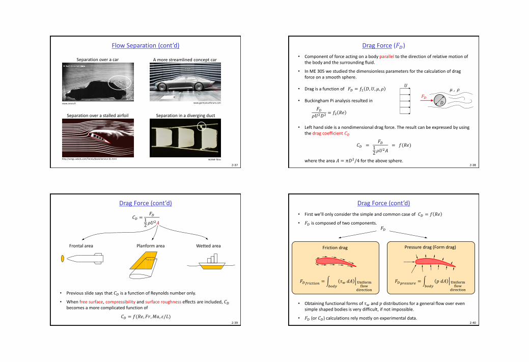
Flow Separation
𝑢/𝑈
𝑦
𝛿
1
010
2-37
Flow Separation (cont’d)
NCFMF filmshttp://wings.avkids.com/Tennis/Book/laminar-01.html
Separation over a stalled airfoil Separation in a diverging duct
www.onera.fr
Separation over a car A more streamlined concept car
www.germancarforum.com
2-38
• Component of force acting on a body parallel to the direction of relative motion of the body and the surrounding fluid.
• In ME 305 we studied the dimensionless parameters for the calculation of drag force on a smooth sphere.
• Drag is a function of 𝐹𝐷 = 𝑓1 𝐷, 𝑈, 𝜇, 𝜌
• Buckingham Pi analysis resulted in
𝐹𝐷
𝜌𝑈2𝐷2= 𝑓2 𝑅𝑒
• Left hand side is a nondimensional drag force. The result can be expressed by using the drag coefficient 𝐶𝐷
𝐶𝐷 =𝐹𝐷
12𝜌𝑈2𝐴
= 𝑓(𝑅𝑒)
where the area 𝐴 = 𝜋𝐷2/4 for the above sphere.
Drag Force (𝐹𝐷)
𝐷
𝑈𝜇 , 𝜌
𝐹𝐷
2-39
𝐶𝐷 =𝐹𝐷
12
𝜌𝑈2𝐴
Drag Force (cont’d)
Frontal area Planform area Wetted area
• Previous slide says that 𝐶𝐷 is a function of Reynolds number only.
• When free surface, compressibility and surface roughness effects are included, 𝐶𝐷
becomes a more complicated function of
𝐶𝐷 = 𝑓(𝑅𝑒, 𝐹𝑟,𝑀𝑎, 휀/𝐿)2-40
• First we’ll only consider the simple and common case of 𝐶𝐷 = 𝑓 𝑅𝑒
• 𝐹𝐷 is composed of two components.
Drag Force (cont’d)
𝐹𝐷
Friction drag
𝐹𝐷𝑓𝑟𝑖𝑐𝑡𝑖𝑜𝑛 = 𝑏𝑜𝑑𝑦
𝜏𝑤 𝑑𝐴 Uniformflow
direction
Pressure drag (Form drag)
𝐹𝐷𝑝𝑟𝑒𝑠𝑠𝑢𝑟𝑒 = 𝑏𝑜𝑑𝑦
𝑝 𝑑𝐴 Uniformflow
direction
• Obtaining functional forms of 𝜏𝑤 and 𝑝 distributions for a general flow over even simple shaped bodies is very difficult, if not impossible.
• 𝐹𝐷 (or 𝐶𝐷) calculations rely mostly on experimental data.

2-41
Drag Force (cont’d)
• Flat plate, when aligned parallel to the flow, is a perfectly streamlined body.
• 𝐹𝐷 on such a plate is purely do to shear forces. Pressure drag is zero.
• When the plate is perpendicular to the flow the extremely blunt case is obtained.
𝐹𝐷 = 𝐹𝐷𝑓𝑟𝑖𝑐𝑡𝑖𝑜𝑛
𝐹𝐷𝑝𝑟𝑒𝑠𝑠𝑢𝑟𝑒 = 0
𝐹𝐷 = 𝐹𝐷𝑝𝑟𝑒𝑠𝑠𝑢𝑟𝑒
𝐹𝐷𝑓𝑟𝑖𝑐𝑡𝑖𝑜𝑛 = 0
Streamlines are almost straight
2-42
Drag Force on a Flat Plate
• Consider flow over a flat plate, with length 𝐿 and width 𝑏.
Blasius’ solution for laminar flow ∶ 𝐶𝐷 =1.328
𝑅𝑒𝐿
(Slide 2−24)
von Karman’s MIA with 𝑛 = 7 profile : 𝐶𝐷 =0.072
𝑅𝑒𝐿1/5
(Slide 2−32)
Schlichting’s formula with transition at 5 × 10⁵ : 𝐶𝐷 =0.455
log 𝑅𝑒𝐿2.58 −
1700
𝑅𝑒𝐿
Completely turb. flow on rough plate : 𝐶𝐷 = 1.89 − 1.62 log휀
𝐿
−2.5
𝐶𝐷 =𝐹𝐷
12𝜌𝑈2𝑏𝐿
𝐿
𝑏
𝑈
Note: Previously we used 𝐶𝑓𝐿 for flat plate.
It′s the same as 𝐶𝐷 .
2-43
• Experimental data is plotted.
• Very similar to the Moody diagram used for pipe flow.
• Laminar flow curve represents Blasius’ exact solution.
• Relative surface roughness(휀/𝐿) becomes a factor in the turbulent regime.
• For high 𝑅𝑒𝐿 values(completely turbulent regime)𝐶𝐷 becomes independent of 𝑅𝑒𝐿, i.e. roughness becomes the only defining parameter.
𝐶𝐷
𝑅𝑒𝐿
𝐶𝐷 for Flow over a Flat Plate
Munson’s book
2-44
Drag Force on a Flat Plate (cont’d)
Exercise : A supertanker is 360 m long, has a beam width of 70 m and a draft of 25 m. Estimate the force and power required to overcome skin friction drag at a cruising speed of 13 knot in seawater at 10 oC.
𝐷 = 25 m
𝑈
Water line (Blue part is under the water)
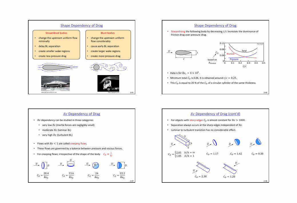
Shape Dependency of Drag
Streamlined bodies
• change the upstream uniform flow minimally
• delay BL separation
• create smaller wake regions
• create less pressure drag
Blunt bodies
• change the upstream uniform flow considerably
• cause early BL separation
• create larger wake regions
• create more pressure drag
2-45http://jalopnik.comwww.germancarforum.com
Shape Dependency of Drag
• Streamlining the following body by decreasing 𝑡/𝑐 increases the dominance of friction drag over pressure drag.
2-46
𝑡
𝑐
𝑈 Total
Pressure
Friction
0 0.1 0.2 0.3 0.4 0.5
𝑡/𝑐
𝐶𝐷
Fox’s book
0.04
0.08
0.12
0based on 𝐴frontal
• Data is for 𝑅𝑒𝑐 = 4 × 10⁵.
• Minimum total 𝐶𝐷 is 0.06. It is obtained around 𝑡/𝑐 = 0.25.
• This 𝐶𝐷 is equal to 20 % of the 𝐶𝐷 of a circular cylinder of the same thickness.
2-47
𝑅𝑒 Dependency of Drag
• 𝑅𝑒 dependency can be studied in three categories.
• very low 𝑅𝑒 (inertia forces are negligibly small)
• moderate 𝑅𝑒 (laminar BL)
• very high 𝑅𝑒 (turbulent BL)
• Flows with 𝑅𝑒 < 1 are called creeping flows.
• These flows are governed by a balance between pressure and viscous forces.
• For creeping flows, irrespective of the shape of the body 𝐶𝐷 ∝1
𝑅𝑒
𝑈𝐷
𝑈
𝐷𝑈 𝐷 𝑈
𝐷
𝐶𝐷 =20.4
𝑅𝑒𝐷𝐶𝐷 =
13.6
𝑅𝑒𝐷𝐶𝐷 =
24
𝑅𝑒𝐷𝐶𝐷 =
22.2
𝑅𝑒𝐷
2-48
𝑅𝑒 Dependency of Drag (cont’d)
• For objects with sharp edges 𝐶𝐷 is almost constant for 𝑅𝑒 > 1000.
• Separation always occurs at the sharp edges independent of 𝑅𝑒.
• Laminar to turbulent transition has no considerable effect.
𝑈
𝑏
𝐶𝐷 = 2.051.05
𝑏 ℎ = ∞ 𝑏 ℎ = 1
ℎ
ℎ 𝑈 𝑈 𝑈
𝐶𝐷 = 1.17 𝐶𝐷 = 1.42 𝐶𝐷 = 0.38
𝑈
𝐶𝐷 = 2.30
𝑈
𝐶𝐷 = 1.20
2-49
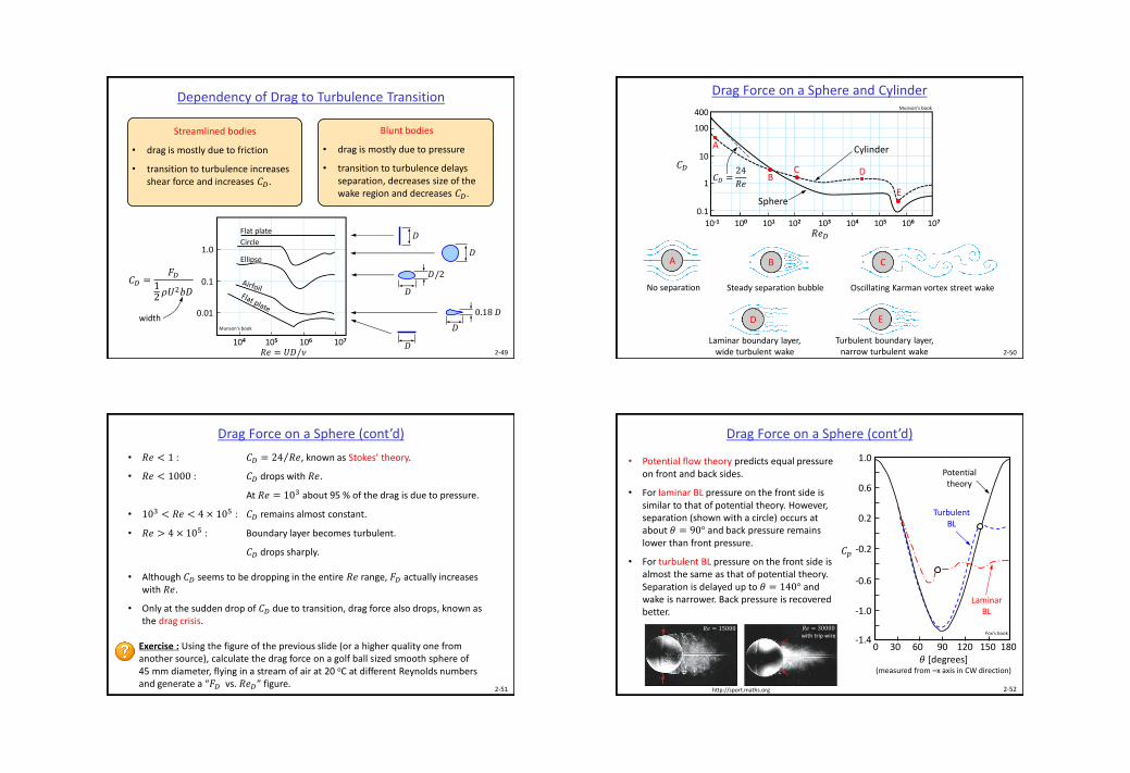
Dependency of Drag to Turbulence Transition
Streamlined bodies
• drag is mostly due to friction
• transition to turbulence increases shear force and increases 𝐶𝐷.
Blunt bodies
• drag is mostly due to pressure
• transition to turbulence delays separation, decreases size of the wake region and decreases 𝐶𝐷.
104 105 106 107
1.0
Flat plate
𝑅𝑒 = 𝑈𝐷/𝜈
𝐶𝐷 =𝐹𝐷
12𝜌𝑈2𝑏𝐷
0.1
0.01
Circle
Ellipse
𝐷
𝐷
𝐷
𝐷
𝐷/2
𝐷
0.18 𝐷
Munson’s book
width
2-50
Drag Force on a Sphere and Cylinder
A B C
D E
No separation Steady separation bubble Oscillating Karman vortex street wake
Laminar boundary layer, wide turbulent wake
Turbulent boundary layer, narrow turbulent wake
10-1 100 101 102 103 104 105 106 107
400
B
100
10
1
0.1
𝐶𝐷
Munson’s book
A
C D
ESphere
Cylinder
𝐶𝐷 =24
𝑅𝑒
𝑅𝑒𝐷
2-51
Drag Force on a Sphere (cont’d)
• 𝑅𝑒 < 1 : 𝐶𝐷 = 24 𝑅𝑒, known as Stokes’ theory.
• 𝑅𝑒 < 1000 : 𝐶𝐷 drops with 𝑅𝑒.
At 𝑅𝑒 = 103 about 95 % of the drag is due to pressure.
• 103 < 𝑅𝑒 < 4 × 10⁵ : 𝐶𝐷 remains almost constant.
• 𝑅𝑒 > 4 × 10⁵ : Boundary layer becomes turbulent.
𝐶𝐷 drops sharply.
• Although 𝐶𝐷 seems to be dropping in the entire 𝑅𝑒 range, 𝐹𝐷 actually increases with 𝑅𝑒.
• Only at the sudden drop of 𝐶𝐷 due to transition, drag force also drops, known as the drag crisis.
Exercise : Using the figure of the previous slide (or a higher quality one from another source), calculate the drag force on a golf ball sized smooth sphere of45 mm diameter, flying in a stream of air at 20 oC at different Reynolds numbers and generate a “𝐹𝐷 vs. 𝑅𝑒𝐷” figure.
2-52
Drag Force on a Sphere (cont’d)
• Potential flow theory predicts equal pressure on front and back sides.
• For laminar BL pressure on the front side is similar to that of potential theory. However, separation (shown with a circle) occurs at about 𝜃 = 90° and back pressure remains lower than front pressure.
• For turbulent BL pressure on the front side is almost the same as that of potential theory. Separation is delayed up to 𝜃 = 140° and wake is narrower. Back pressure is recovered better.
0 30 60 90 120 150 180
Fox’s book
𝜃 [degrees](measured from –x axis in CW direction)
𝐶𝑝
1.0
0.6
0.2
-0.2
-0.6
-1.0
-1.4
Potential theory
Laminar BL
Turbulent BL
http://sport.maths.org
𝑅𝑒 = 15000 𝑅𝑒 = 30000with trip wire

2-53
Drag Force on a Sphere (cont’d)
• For a smooth sphere transition of BL flow into turbulence occurs at about 4 × 10⁵.
• For a rough sphere transition occurs at lower 𝑅𝑒 values.
4x10⁴ 105 4x10⁵ 106 4x10⁶
0.1
𝐶𝐷 a
𝑅𝑒𝐷
0.2
0.3
0.4
0.5
0.6
b
cd
e Relative roughness 휀 𝐷 is equal to
a ∶b ∶c ∶d ∶e ∶
that of a golf ball0.01250.0050.0015smooth
Munson’s book
2-54
Drag Force on a Sphere – Effect of Surface Roughness (cont’d)
• Dimples on a golf ball are carefully designed such that they “trip” the BL flow into turbulence at 𝑅𝑒 = 4 × 10⁴ , which is precisely the 𝑅𝑒 value of a well-hit golf ball.
• A smooth golf ball can at most be hit to approximately 120 m. A dimpled one can fly up to 265 m.
• For a smooth sphere, transition to turbulence reduces 𝐶𝐷 by a factor of 5.
• For a golf ball, transition to turbulence reduces 𝐶𝐷 by a factor of 2. But the important point is that the reduction takes place at a lower 𝑅𝑒, matching the 𝑅𝑒of a flying golf ball.
Exercise : Watch the Mythbusters episode about “Fuel Efficiency of a Dimpled Car” and read about a “CFD Study on Golf Ball Aerodynamics”.
http://dsc.discovery.com/videos/mythbusters-dimpled-car-minimyth.html
http://www.newswise.com/articles/view/546607
2-55
Effect of Mach Number on 𝐶𝐷
• For subsonic with low Mach number, 𝐶𝐷 is not a function of 𝑀𝑎.
• But it increases sharply after a certain 𝑀𝑎 value.
• Following figure shows the variation of 𝐶𝐷 with 𝑀𝑎 for two objects of width 𝑏. First object has a square cross section.
𝐶𝐷 =𝐹𝐷
12 𝜌𝑈2𝑏𝐷
3.0
2.5
2.0
1.5
1.0
0.5
00.5 1.00
𝐷
4𝐷
𝐷
𝑀𝑎
Munson’s book
reference density
𝑈
𝑈
width
2-56
Effect of Mach Number on 𝐶𝐷 (cont’d)
• For supersonic flows formation of shock waves plays an important role.
• Detached, bow shocks form in front of blunt bodies.
• Attached shocks form on the leading edge of pointed bodies.
𝐶𝐷 =𝐹𝐷
12 𝜌𝑈2 𝜋𝐷2
4
1.2
0.8
0.4
030
𝐷
𝑀𝑎
Munson’s book
1.6
1 2 4
𝐷
circular cylinder
cylinderwith sharpnose
𝑈
𝑈

2-57
Effect of Mach Number on 𝐶𝐷 (cont’d)
• Schlieren images of shock waves in high speed flight of blunt and pointed bodies.
http://qdl.scs-inc.us web.mit.edu
www.nasa.gov 2-58
Effect of Froude Number on 𝐶𝐷
• For objects moving on a free surface wave drag becomes important.
• Hull shapes of ships are designed to reduce wave drag.
• Use of a bulbous bow creates extra waves that cancel out the waves generated by the hull and reduce wave drag considerably.
𝐶𝐷𝑤𝑎𝑣𝑒=
𝐹𝐷
12𝜌𝑈2𝐿2
0.0010
00.30.1
𝐹𝑟 = 𝑈/ 𝐿𝑔
Munson’s book0.0015
0.0005
0.2 0.4
𝐿
𝐿
bulbous bow
2-59
Effect of Froude Number on 𝐶𝐷 (cont’d)
• Bulbous bows used for wave drag reduction.
www.cruiseradio.net
www.globalsecurity.org
2-60
Composite Drag
• Approximate drag estimate of a complex body can be done by treating the body as an assembly of simpler parts. See the distributed handout.
• For example for an airplane, drag on the fuselage, wings and tail can be estimated separately and added.
• Interaction between various parts affect the accuracy of the analysis.
Exercise : A 95 km/h wind blows past a water tower. Estimate the wind force actingon it (Reference: Munson).
𝑈
𝑏
𝐷𝑠
𝐷𝑐
𝑈 = 95 km/h
𝐷𝑠 = 12 m
𝐷𝑐 = 4.5 m
L= 15 m

Lift Force
• Lift is the component of the force that is perpendicular to the flow direction.
𝐶𝐿 =𝐹𝐿
12
𝜌𝑈2𝐴
Planform area (𝐴 = 𝑏𝑐)
2-61
Lift coefficient
Planformarea = 𝑏𝑐
ThicknessSpan (𝑏)
Angle of attack (𝛼)
𝑈
2-62
Lift Force (cont’d)
• An airfoil can generate lift because of the low and high pressures on its top and bottom surfaces, respectively.
• Pressure distribution over an airfoil is usually given as a 𝐶𝑝 graph.
Compressible flow with a shock over RAE 2822 airfoil
𝑀𝑎 = 0.729
𝛼 = 2.31°
Shock is at the uppersurface at about
𝑥/𝑐 = 0.55
𝐶𝑝 =𝑝 − 𝑝∞
12
𝜌∞𝑈∞2
𝑥/𝑐
-1.5
0.0 0.2 0.4 0.6 0.8 1.0
-1.0
-0.5
0.0
0.5
1.0
Top surface
Bottom surface
www.grc.nasa.gov
2-63
Lift Force (cont’d)
• 𝐶𝐿 increases with angle of attack up to stall. 𝐶𝐷 also increases with angle of attack.
Fox’s book
As 𝛼 increases, separation point on the top surface moves towards the leading edge. At stall, separation occurs at a major portion of the top surface and lift drops sharply.
𝐶𝐿
1.8
𝑈
1.6
1.4
1.2
1.0
0.8
0.6
0.4
0.2
00 4 8 12 16 20
𝛼
NACA 23015airfoil
𝛼 (deg)
𝐶𝐷
0.020
0.016
0.012
0.008
0.004
00 4 8 12 16 20
NACA 23015airfoil
𝛼 (deg)2-64
Lift Force (cont’d)
• Flaps are movable portions of a wing trailing edge that may be extended during landing and takeoff to increase effective wing area.
• They increase 𝐶𝐿 considerably at a given 𝛼. But they also increase 𝐶𝐷 and are not used during normal cruising.
Fox’s book
𝐶𝐿
3.5
-5 0 5 10 15 20
𝛼 (deg)
3.0
2.5
2.0
1.5
1.0
0.5
3
2
1𝐶𝐿
3.5
0 0.1 0.2 0.3
𝐶𝐷
3.0
2.5
2.0
1.5
1.0
0.5
3
2
1
3. Doubleslotted flap
2. Slotted flap
1. No flap
2-65
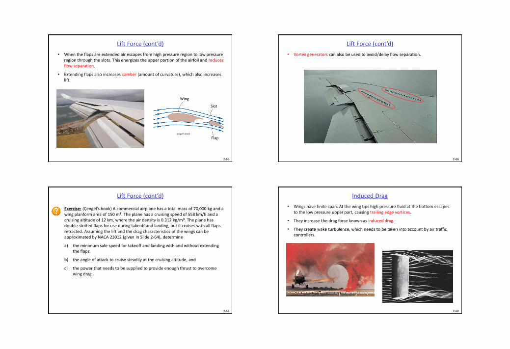
Lift Force (cont’d)
• When the flaps are extended air escapes from high pressure region to low pressure region through the slots. This energizes the upper portion of the airfoil and reduces flow separation.
• Extending flaps also increases camber (amount of curvature), which also increases lift.
Çengel’s book
Wing
Slot
Flap
2-66
• Vortex generators can also be used to avoid/delay flow separation.
Lift Force (cont’d)
2-67
Exercise: (Çengel’s book) A commercial airplane has a total mass of 70,000 kg and a wing planform area of 150 m2. The plane has a cruising speed of 558 km/h and a cruising altitude of 12 km, where the air density is 0.312 kg/m3. The plane has double-slotted flaps for use during takeoff and landing, but it cruises with all flaps retracted. Assuming the lift and the drag characteristics of the wings can be approximated by NACA 23012 (given in Slide 2-64), determine
a) the minimum safe speed for takeoff and landing with and without extending the flaps,
b) the angle of attack to cruise steadily at the cruising altitude, and
c) the power that needs to be supplied to provide enough thrust to overcome wing drag.
Lift Force (cont’d)
2-68
Induced Drag
• Wings have finite span. At the wing tips high pressure fluid at the bottom escapes to the low pressure upper part, causing trailing edge vortices.
• They increase the drag force known as induced drag.
• They create wake turbulence, which needs to be taken into account by air traffic controllers.
2-69
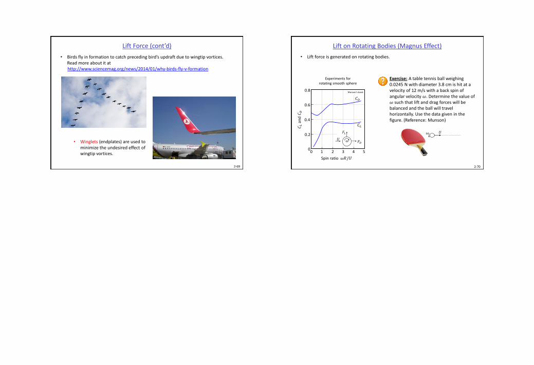
Lift Force (cont’d)
• Birds fly in formation to catch preceding bird’s updraft due to wingtip vortices. Read more about it athttp://www.sciencemag.org/news/2014/01/why-birds-fly-v-formation
• Winglets (endplates) are used to minimize the undesired effect of wingtip vortices.
2-70
Lift on Rotating Bodies (Magnus Effect)
• Lift force is generated on rotating bodies.
𝐹𝐿
𝜔𝑈
𝐶𝐿
and
𝐶𝐷
Spin ratio 𝜔𝑅/𝑈
0 1 2 3 4 5
0.8
𝐶𝐿
𝐶𝐷
Experiments for rotating smooth sphere
Munson’s book
𝐹𝐷
0.6
0.4
0.2
0
Exercise: A table tennis ball weighing 0.0245 N with diameter 3.8 cm is hit at a velocity of 12 m/s with a back spin of angular velocity 𝜔. Determine the value of 𝜔 such that lift and drag forces will be balanced and the ball will travel horizontally. Use the data given in the figure. (Reference: Munson)
𝜔 𝑈