1

BORN-INFELD GRAVITY THEORIES IN D-DIMENSIONS

A THESIS SUBMITTED TOTHE GRADUATE SCHOOL OF NATURAL AND APPLIED SCIENCES

OFMIDDLE EAST TECHNICAL UNIVERSITY

BY

TAHSIN CAGRI SISMAN

IN PARTIAL FULFILLMENT OF THE REQUIREMENTSFOR

THE DEGREE OF DOCTOR OF PHILOSOPHYIN

PHYSICS

SEPTEMBER 2012

Approval of the thesis:

BORN-INFELD GRAVITY THEORIES IN D-DIMENSIONS

submitted by TAHSIN CAGRI SISMAN in partial fulfillment of the requirementsfor the degree of Doctor of Philosophy in Physics Department, Middle EastTechnical University by,

Prof. Dr. Canan OzgenDean, Graduate School of Natural and Applied Sciences

Prof. Dr. Mehmet ZeyrekHead of Department, Physics

Prof. Dr. Bayram TekinSupervisor, Physics Dept., METU

Examining Committee Members:

Prof. Dr. Metin GursesMathematics Dept., Bilkent University

Prof. Dr. Bayram TekinPhysics Dept., METU

Prof. Dr. Bahtiyar Ozgur SarıogluPhysics Dept., METU

Assoc. Prof. Dr. Konstantin ZheltukhinMathematics Dept., METU

Prof. Dr. Atalay KarasuPhysics Dept., METU

Date:

I hereby declare that all information in this document has been obtainedand presented in accordance with academic rules and ethical conduct. Ialso declare that, as required by these rules and conduct, I have fully citedand referenced all material and results that are not original to this work.

Name, Last Name: TAHSIN CAGRI SISMAN

Signature :

iii

ABSTRACT

BORN-INFELD GRAVITY THEORIES IN D-DIMENSIONS

Sisman, Tahsin CagrıPh.D., Department of Physics

Supervisor : Prof. Dr. Bayram Tekin

September 2012, 100 pages

Born-Infeld gravity proposed by Deser and Gibbons takes its origin from two ideas:

Born-Infeld electrodynamics and Eddington’s gravitational action. The theory is de-

fined with a determinantal action involving the Ricci tensor as in the Eddington’s

theory; however, in contrast, the independent variable is the metric as in Einstein’s

gravity and the action is constructed in analogy with the action of the Born-Infeld

electrodynamics. Main challenge in defining a Born-Infeld type gravity is obtaining

a unitary theory around–at least–flat and maximally symmetric constant curvature

backgrounds. In this thesis, a framework for analyzing the tree-level unitarity of a

generic D-dimensional Born-Infeld type gravity is developed. Besides, in three dimen-

sions, a Born-Infeld gravity theory which is unitary to all orders in the curvature is

studied in detail. This theory was introduced as an extension of a specific quadratic

curvature gravity theory dubbed as “new massive gravity” which is unitary with a

massive spin-2 excitation in its spectrum. Besides having a unitary massive spin-2

excitation, the Born-Infeld gravity in three dimensions has a holographic c-function

which is the same as Einstein’s gravity. In addition, the theory has constant curvature

Type-N and Type-D solutions which are the same as the cosmological topologically

massive gravity.

iv

Keywords: Born-Infeld gravity, new massive gravity, topologically massive gravity,

Type-N solutions, Type-D solutions

v

OZ

D-BOYUTTA BORN-INFELD KUTLECEKIM TEORILERI

Sisman, Tahsin CagrıDoktora, Fizik Bolumu

Tez Yoneticisi : Prof. Dr. Bayram Tekin

Eylul 2012, 100 sayfa

Deser ve Gibbons tarafından ortaya atılmıs olan Born-Infeld kutlecekim, kaynagını

Born-Infeld elektrodinamigi ve Eddington’un kutlecekim eylemi fikirlerinden almak-

tadır. Teori, Eddington’un teorisinde oldugu gibi Ricci tensorunun determinantını

iceren bir eylemle tanımlanır, fakat bu teoriden farklı olarak Einstein teorisinde oldugu

gibi bagımsız degisken metriktir ve eylem Born-Infeld elektrodinamiginin eylemiyle

analoji uzerinden kurulur. Born-Infeld tipi kutlecekim tanımlanırken karsılasılan

temel zorluk (en azından) duz ve maksimal olarak simetrik sabit egrilikli arkaplanlar

etrafında uniter bir teori elde edilmesi geregidir. Bu tezde, D-boyutlu genel Born-

Infeld tipi kutlecekimin agac mertebesi uniterligini analiz etmek icin gerekli cerceve

gelistirilecektir. Buna ek olarak, uc boyutta egrilik terimlerinin butun mertebeleri icin

uniter olan Born-Infeld kutlecekim teorisi detaylı bir sekilde incelenecektir. Bu teori,

“yeni kutleli gravitasyon” olarak adlandırılan, uniter, spekturumunda kutleli spin-2

tedirgemeler olan ozel bir ikinci dereceden egrilikli kutlecekim teorisinin genisletilmesi

olarak ortaya atılmıstır. Uc boyuttaki Born-Infeld kutlecekim teorisi, uniter kutleli

spin-2 tedirgemeler icermesinin yanında Einstein kutlecekim ile aynı holografik c-

fonksiyonuna sahiptir. Ek olarak, bu teori kozmolojik sabitli topolojik kutleli gravi-

tasyon ile aynı Tip-N ve Tip-D cozumlerine sahiptir.

vi

Anahtar Kelimeler: Born-Infeld kutlecekim, yeni kutleli kutlecekim, topolojik kutleli

kutlecekim, Tip-N cozumler, Tip-D cozumler

vii

To Kiraz, my dear wife

viii

ACKNOWLEDGMENTS

First of all, I would like to gratefully and sincerely thank my supervisor Professor

Bayram Tekin. In the real sense of the phrase, words cannot express my appreciation

to him. If my dream to become a physicist come true, it will be mainly due to him.

He not only taught me physics, but also helped me to gain a scientific perspective. I

have learned from him to hard work day and night, to have a courage to attack the

hardest problems and how to get an insight into the core points of a physical concept

or phenomena. He has been always supportive and patient since the beginning of my

PhD study. My case is a real example of the fact that the important choice is not the

choice of the graduate school, but the choice of the supervisor.

I also would like to thank Professor Metin Gurses for the opportunity to collaborate

with him. His lifelong curiosity and unflagging manner in doing calculations will

always effect me. In addition, I am indebted to Professor Atalay Karasu, Professor B.

Ozgur Sarıoglu, Professor Ayse Kalkanlı Karasu and Professor Altug Ozpineci for the

courses that shaped my knowledge as a theoretical physicist and for their guidance

during my undergraduate and graduate study at METU.

I am thankful to Dr. Ibrahim Gullu for his collaboration lasting more than two years.

During this period, I have learned a lot on gravitational physics from and with him.

In addition, I have also learned from the discussions on gravitational physics with

Sinan Deger, Suat Dengiz, Deniz Olgu Devecioglu, Ulas Huyal, Burak Ilhan, Mehmet

Ali Olpak, Sener Ozonder, Emre Sakarya, and Cetin Senturk. I am thankful to them

all.

The summer schools that I have attended, especially the ones at the Feza Gursey

Institute, were very crucial in my PhD education. I am indebted to the organizers of

the summer schools at the Feza Gursey Institute, namely, Professor Haji Ahmedov,

Professor Levent Akant, Professor A. Nihat Berker, Professor Altug Ozpineci, Profes-

sor Teoman Turgut, and Professor Kayhan Ulker. Surely, the unfortunate termination

ix

of the Feza Gursey Institute will be a great loss in the education of future generations

of theoretical physicists in Turkey. In addition, I am thankful to The Abdus Salam

International Centre for Theoretical Physics and Ettore Majorana Foundation and

Centre for Scientific Culture for the support they provided to attend the scientific

activities in these centers.

I would like to thank to Professor Kasper Peeters for providing the computer algebra

system Cadabra as a free software to high energy physics community. I have done or

verified some of the calculations in this thesis with this powerful software.

I am grateful to my wife for her patience during this study and without her support,

this work cannot be done. Also, I would like to thank my father for his guidance

and together with him to my sister and uncle for their support during all of my

education. Last but not the least, I would like to thank my mother. Her courage and

her ambitious nature shaped my character and motivates me to go further.

During my PhD study, I have been supported by TUBITAK with a 2211 PhD schol-

arship in the first five years and with a PhD scholarship in the 1001 project 110T339

in the final two years.

x

TABLE OF CONTENTS

ABSTRACT . . . . . . . . . . . . . . . . . . . . . . . . . . . . . . . . . . . . . iv

OZ . . . . . . . . . . . . . . . . . . . . . . . . . . . . . . . . . . . . . . . . . . . vi

ACKNOWLEDGMENTS . . . . . . . . . . . . . . . . . . . . . . . . . . . . . . ix

TABLE OF CONTENTS . . . . . . . . . . . . . . . . . . . . . . . . . . . . . . xi

LIST OF FIGURES . . . . . . . . . . . . . . . . . . . . . . . . . . . . . . . . . xiii

CHAPTERS

1 INTRODUCTION . . . . . . . . . . . . . . . . . . . . . . . . . . . . . 1

1.1 Born-Infeld gravity . . . . . . . . . . . . . . . . . . . . . . . . 3

1.2 Tree-level unitarity . . . . . . . . . . . . . . . . . . . . . . . . 5

1.2.1 Propagator Structure of Quadratic Curvature Gravity 8

2 UNITARITY ANALYSIS OF BORN-INFELD GRAVITY THEORIES 14

2.1 BI-Type Actions at O(h2) . . . . . . . . . . . . . . . . . . . . 16

2.1.1 General analysis . . . . . . . . . . . . . . . . . . . . . 16

2.1.2 O (h) equivalence in two dimensions . . . . . . . . . . 29

2.1.3 Unitarity analysis of BI gravity Aµν = αRµν in D = 4 32

2.2 Equivalent Quadratic Curvature Actions . . . . . . . . . . . . 38

2.2.1 Analysis of cubic order of BI gravity Aµν = αRµν . . 41

2.2.2 Analysis of BI gravity Aµν = αRµν . . . . . . . . . . 43

2.3 Unitarity analysis of Born-Infeld Gravity Proposed by Deserand Gibbons . . . . . . . . . . . . . . . . . . . . . . . . . . . . 44

3 BORN-INFELD EXTENSION OF NEW MASSIVE GRAVITY . . . . 47

3.1 Constructing the Born-Infeld extension of New Massive Gravity 47

3.2 Unitarity around (A)dS and central charge . . . . . . . . . . . 51

3.3 Exact solutions . . . . . . . . . . . . . . . . . . . . . . . . . . 57

xi

3.3.1 Classification of three-dimensional spacetimes . . . . 58

3.3.2 Field equations of TMG and NMG for Type-N andType-D spacetimes . . . . . . . . . . . . . . . . . . . 60

3.3.3 Field Equations of BINMG . . . . . . . . . . . . . . . 64

3.3.4 Type-N solutions . . . . . . . . . . . . . . . . . . . . 66

3.3.5 Type-D solutions . . . . . . . . . . . . . . . . . . . . 68

3.4 Holographic c-theorem . . . . . . . . . . . . . . . . . . . . . . 71

3.4.1 c-functions . . . . . . . . . . . . . . . . . . . . . . . . 72

3.4.2 Weyl anomaly . . . . . . . . . . . . . . . . . . . . . . 76

4 CONCLUSIONS . . . . . . . . . . . . . . . . . . . . . . . . . . . . . . 78

REFERENCES . . . . . . . . . . . . . . . . . . . . . . . . . . . . . . . . . . . . 80

APPENDICES

A EXPANSIONS IN METRIC PERTURBATION . . . . . . . . . . . . . 84

A.1 Second Order Expansions of Curvature Tensors . . . . . . . . 84

A.2 Some linearization results in four dimensions . . . . . . . . . . 86

A.3 Variations of cubic curvature terms . . . . . . . . . . . . . . . 86

B ANALYZING EINSTEIN’S GRAVITY AND QUADRATIC CURVA-TURE GRAVITY WITH SECOND ORDER PERTURBATIONS . . 88

B.1 Analysis of Einstein’s gravity . . . . . . . . . . . . . . . . . . . 88

B.2 Analysis of quadratic curvature gravity . . . . . . . . . . . . . 90

CURRICULUM VITAE . . . . . . . . . . . . . . . . . . . . . . . . . . . . . . . 95

xii

LIST OF FIGURES

FIGURES

Figure 1.1 Tree-level scattering amplitude between two background covariantly

conserved sources via the exchange of a graviton . . . . . . . . . . . . . . . 9

Figure 3.1 The first graph gives a possible behavior for A′ (r) in the σ = +1

case, while the second one shows a possible behavior for A′ (r) in the σ = −1

case. . . . . . . . . . . . . . . . . . . . . . . . . . . . . . . . . . . . . . . . 74

xiii

CHAPTER 1

INTRODUCTION

General relativity represents our current understanding of gravitation and at solar sys-

tem scales, it is a well-tested theory. However, in larger scales, various observations

imply a possible modification of the theory. For example, the accelerated expansion of

the Universe can be explained by augmenting Einstein’s gravity with a cosmological

constant. Furthermore, the observations suggesting the existence of dark matter may

also be an indication of a modification in the gravitational laws. In addition to this

observational motivations, there are also theoretical considerations implying a modifi-

cation of Einstein’s gravity. Reconciling general relativity with quantum mechanics is

a major theoretical problem and the nonrenormalizability of Einstein’s gravity is an

important issue in this respect. In various quantum gravity scenarios, such as string

theory, asymptotic safety, Einstein’s gravity appears as a low energy effective field

theory which should be augmented by higher derivative terms to cure the nonrenor-

malizability behavior. Indeed, the extension of the theory with quadratic curvature

terms was shown to be renormalizable [1]; however, the corresponding quantum theory

is not unitary [1, 2]. With the effective field theory perspective, the generic form of

the gravitational action is

I =∫d4x

{1κ

(R− 2Λ0) +∞∑n=2

an (Riem, Ric, R, ∇Riem, . . . )n}, (1.1)

and the question is that which higher derivative and higher curvature terms appear

in this action with which couplings. One may try to deduce the possible higher order

terms and their couplings from a proposal of a UV-complete fundamental theory

describing the quantum gravity. On the other hand, instead of this top-down approach,

it is possible to consider various theoretical consistency requirements such as unitarity

1

and try to figure out constraints on the possible terms and their couplings. In this

regard, extending Einstein’s gravity with higher curvature terms and studying viability

of these theories can help to get general constraints on (1.1).

In this thesis, we focus on Born-Infeld gravity which is a specific infinite order higher

curvature modification of Einstein’s gravity. The bulk of the material presented here

is based on the original research work whose results were published in the papers:

• I. Gullu, T. C. Sisman, B. Tekin, “Born-Infeld extension of new massive gravity”

[3],

• I. Gullu, T. C. Sisman and B. Tekin, “c-functions in the Born-Infeld extended

New Massive Gravity” [4],

• I. Gullu, T. C. Sisman and B. Tekin, “Unitarity analysis of general Born-Infeld

gravity theories” [5],

• I. Gullu, T. C. Sisman, B. Tekin, “All Bulk and Boundary Unitary Cubic Cur-

vature Theories in Three Dimensions” [6],

• M. Gurses, T. C. Sisman and B. Tekin, “Some exact solutions of all f (Rµν)

theories in three dimensions” [7].

Our main aim is to study the theoretical consistency of D-dimensional Born-Infeld

gravity theories and to discuss a particularly successful three-dimensional Born-Infeld

gravity theory.

The layout of this thesis is as follows: In the remaining sections of this chapter, first, we

give a brief introduction on Born-Infeld gravity theories, and then, we discuss the tree-

level unitarity of higher curvature gravity theories. In the second chapter, we analyze

the unitarity of D-dimensional Born-Infeld gravity theories. Third chapter is devoted

to the three-dimensional Born-Infeld gravity theory and its properties. A conclusion

chapter is followed by two appendices on the metric perturbation expansions of various

tensorial structures and the perturbative analysis of the quadratic curvature gravity

action.

Now, let us give our conventions. The signature of the metric is taken to be mostly

positive. The Riemann tensor is defined as Rµνρσ ≡ ∂ρΓµσν + ΓµρλΓλσν − ρ ↔ σ, while

2

the Ricci tensor is Rνσ ≡ Rµνµσ. The determinant of the metric gµν is denoted as g.

To avoid a possible confusion, the determinants of rank-(0, 2) and rank-(1, 1) tensors

are shown explicitly; for example, as det (gµν +Aµν) and det (δµν +Aµν ).

1.1 Born-Infeld gravity

The idea of the Born-Infeld (BI) type modifications of Einstein’s gravity was proposed

by Deser and Gibbons [8]. As the name suggests, the theory has common features

with Born-Infeld electrodynamics [9]. In addition, Eddington’s gravitational action

[10] is the other source of inspiration for the proposal in [8].

BI electrodynamics is based on the principle of finiteness [9]. Born and Infeld consid-

ered the divergences in Maxwell electrodynamics as the failure of the theory and they

defined their theory with the action having a determinantal form as

I = −b2∫d4x

√−det

(gµν + 1

bFµν

), (1.2)

which originated from the relativistic point particle action I = −m∫dt√

1− v2. In

the BI electrodynamics, there is an upper bound for the field strength whose scale is

determined by the dimensionful parameter b. The finiteness of the field strength is

due to the nonlinear nature of the theory and for small field strengths, the BI action

generates the Maxwell action. Furthermore, the excitations of the theory, namely

photons, are not ghost.

Determinantal actions also appeared as a modification of Einstein’s gravity. The

early proposal of Eddington [10], which even predates the BI electrodynamics, was

motivated by the idea of writing a gravitational theory which has the connection as the

fundamental geometric quantity rather than the metric. Then, Eddington preferred to

write a generalized invariant volume element in the form∫d4x

√det

[R(µν) (Γ)

]and

proposed it as the action of the gravitational theory.

Following the ideas of Born and Infeld, and Eddington, the gravitational action

I =∫d4x

√−det (agµν + bRµν + cXµν), (1.3)

was proposed in [8]. Here, a, b, and c are the parameters of the theory. The action

is a generalized invariant volume element which is constructed in a similar form to

3

(1.2). As opposed to Eddington’s action, the fundamental geometric quantity in (1.3)

is the metric. In addition, the tensor Xµν is unknown and should be determined in

such a way that the theory has a consistent spectrum which is free from ghosts and

tachyons. There could of course be more constraints on the theory, such as being

supersymmetrizable, but here we shall be only interested in the unitarity about flat

and (anti)-de Sitter [(A)dS] backgrounds.

In three dimensions, there is a particularly successful example of BI-type gravity

theories whose action has a rather elegant form as [3]

IBINMG = −4m2

κ2

∫d3x

[√−det

(gµν −

1m2Gµν

)−(

1− λ02

)√−g], (1.4)

where Gµν is the Einstein tensor, Gµν ≡ Rµν − 12gµνR. When this action is expanded

in curvature, at the quadratic curvature order, it reproduces new massive gravity

(NMG) theory defined with the action [11, 12]

INMG = 1κ2

∫d3x√−g

[−R− 2λ0m

2 + 1m2

(RµνR

νµ −

38R

2)]

, (1.5)

which is the unique quadratic curvature theory that is unitary around both flat and

(A)dS backgrounds with a massive spin-2 excitation [12, 13, 14, 15, 16].1 This feature

of (1.4) was the original motivation for the construction of (1.4), so the theory was

named as the Born-Infeld extension of NMG (BINMG) [3]. Just like NMG, BINMG is

also unitary around both flat and (A)dS backgrounds with a massive spin-2 excitation

[6], and in fact, BINMG is the first example of a unitary BI-type gravity around the

(A)dS background. Both NMG and BINMG represent nonlinear generalizations of

the Fierz-Pauli massive spin-2 theory which are free from the Boulware-Deser ghost

[18] as shown in [19] for NMG and in [20] for BINMG. As in the case of BI electro-

dynamics for which there is a bound on the maximum attainable field strength, (1.4)

puts a constraint on the curvature as R ≥ −6m2 for (A)dS spacetimes [21]. In addi-

tion, at cubic and quartic orders, the curvature expansion of (1.4) matches the cubic

and the quartic curvature extensions of NMG which were constructed by AdS/CFT

considerations in [22]. Certain aspects of BINMG such as its central charge [23, 4],

c-functions [4], classical solutions [23, 24, 25, 7, 27], and Weyl invariant extension [28]1 Initially, NMG was thought to be renormalizable since the four-dimensional quadratic curvature

theory is renormalizable. However, a careful study reveals that this is not the case for NMG due tothe specific relation satisfied by the couplings of the quadratic curvature terms [17].

4

have been studied. Remarkably, BINMG has a holographic c-function which matches

the c-function of Einstein’s gravity. Furthermore, the gravitational charges for the

BTZ black hole of BINMG were studied in [23, 29]. In addition, as a curious side

remark let us note that BINMG appears as a cut-off independent counterterm to the

four dimensional anti-de Sitter space [30].

1.2 Tree-level unitarity

A gravity theory has a physically consistent spectrum at the tree level if the spectrum is

free from ghosts and tachyons. Ghosts are negative kinetic energy modes. A physically

consistent mode is described with an action I =∫dtL =

∫dt (K − U), where K and

U represent kinetic and potential energies, respectively. Then, the corresponding

Hamiltonian, which represents the energy of the mode, is given as H = K + U , and

it is positive definite for a positive-definite potential. However, for a ghost mode, one

has I =∫dt (−K − U) yielding H = −K + U , so the energy of the ghost mode is

not positive definite. For such a case, the vacuum is not stable and the proliferation

of negative energy modes is entropically favorable. An important feature of ghost

instability is that it is relevant at all energy scales. In addition, the ghost modes

correspond to the negative norm states in the Hilbert space of the corresponding

quantum theory as 〈ψ|H |ψ〉 = −E 〈ψ|ψ〉 ⇒ 〈ψ|ψ〉 = −1. Therefore, the unitarity

of the theory is spoiled by the ghost modes as probabilities are not positive definite

in the presence of negative norm states. On the other hand, tachyons have negative

squared masses.2 To understand the instability caused by tachyons, let us consider

the example of a scalar field φ with the action I [φ] =∫dt [K (∂µφ)− U (φ)]. If one

considers the field fluctuation ϕ ≡ φ − φ around the vacuum φ, that is[dUdφ

]φ

= 0,

then one gets the action

I [ϕ] =∫dt

K (∂µϕ)− U (ϕ)− 12

[d2U

dφ2

]φ

ϕ2 + . . .

,where, as usual,

[d2Udφ2

]φ

corresponds to m2. Thus, a tachyon, which is a negative

m2 mode, corresponds to a unstable vacuum as[d2Udφ2

]φ< 0. Note that the tachyon

2 Note that in AdS if certain bounds are satisfied for various spins, a negative squared mass modeis allowed.

5

instability becomes relevant at energy scales close to m. To sum up, to have a phys-

ically consistent spectrum, excitations of a field theory should have correct signs at

the action level. For example, for a scalar mode, the correct signs of the kinetic term

and the mass term are given with the action I = −12∫d4x

(∂µϕ∂

µϕ+m2ϕ2) for the

mostly plus convention of the metric. It is also possible to read these signs at the

propagator level where one should have 1p2+m2 for a physically consistent scalar mode.

In this thesis, we study the unitarity of BI gravity theories which are infinite order

higher curvature gravity theories with fixed couplings. To analyze the spectrum and

its consistency for a higher curvature gravity theory, one needs to determine the free

theory of metric fluctuations around a background spacetime (or, in other words, a

vacuum) which solves the field equations of the higher curvature gravity theory. The

free theory is described by the second order action in metric fluctuations around the

background and in this study, the background is taken to be either the flat or the

(A)dS spacetime.

In calculating the second order action in metric fluctuations, it is important to observe

that for the flat background higher curvature terms beyond the quadratic curvature

order do not yield any contribution, while for the (A)dS background all the terms in a

higher curvature gravity action contribute in principle. Due to this fact the unitarity

analysis of a higher curvature theory around the (A)dS background is a nontrivial

task. To understand this better, let us consider the example of the cubic curvature

term R3. If the scalar curvature has the expansion in metric fluctuations as

R = R+R(1) +R(2) + . . . , (1.6)

where R(1) and R(2) represent first and second orders of R in metric fluctuations and

R is the background value of R, then the second order contributions that come from

R3 have the forms RR2(1) and R2R(2). Thus, for the flat background these terms

become zero, while for the (A)dS background there are contributions to the second

order action coming from the term R3.

Another important observation in calculating the second order action in metric fluctu-

ations around the (A)dS background is that the contributions coming from the terms

beyond the quadratic curvature order have the same structure as the contributions

coming from the quadratic curvature terms. To understand this point, let us resort

6

to the R3 example again. As discussed above the second order contributions coming

from R3 have the forms RR2(1) and R2R(2), while the second order contributions com-

ing from R2 are R2(1) and RR(2). Thus, the term R3 yields the same forms except

the overall R multiplicity. In the same manner, the independent quadratic curvature

scalars R2, RµνRνµ, and RµνρσRρσµν determine the structure of the second order action and

a higher curvature term of order n yields second order contributions which are the

same as the ones that can come from these three quadratic curvature scalars except

an overall factor proportional to Rn−2. Instead of RµνρσRρσµν , the Gauss-Bonnet (GB)

combination can also be considered as one of the independent scalars. Note that the

GB combination is a boundary term in four dimensions and identically zero in three

dimensions, so the GB combination (or the term RµνρσRρσµν) is relevant in dimensions

greater than four.

Due to these two observations, the unitarity analysis of the most general quadratic

curvature theory defined with the action

I =∫dDx√−g[

1κ

(R− 2Λ0)

+ αR2 + βRµνRνµ + γ

(RµνρσR

ρσµν − 4RµνRνµ +R2

)], (1.7)

lay down the ground rules for the unitarity analysis of higher curvature theories. A

higher curvature theory is unitary if and only if its propagator reduces to the propaga-

tor of one of the known unitary theories at the linear or the quadratic curvature order;

therefore, it is essential to discuss unitary theories of quadratic curvature. For the flat

background, the unitarity of the most general quadratic curvature theory in four di-

mensions was discussed in [2] and it was shown that the quadratic curvature theory

is not unitary in the presence of the term RµνRνµ. This result can be generalized to

higher dimensions; however, in three dimensions, a subtlety occurs and one has NMG

[11] for specific values of the parameters. For the (A)dS background, the unitarity of

(1.7) is studied in [15] where the analysis is in D dimensions. Let us summarize the

results of [2, 11, 15]:

• For D = 4, Einstein’s gravity is unitary around both flat and (A)dS backgrounds

with a massless spin-2 mode. When R2 term is augmented to the Einstein’s grav-

ity, the theory is unitary with an additional massive spin-0 degree of freedom.

7

The original motivation for augmenting Einstein’s gravity with the quadratic

curvature terms is to endow it with renormalizability; however, its R2 extension

is not renormalizable, too. To have a renormalizable quadratic curvature the-

ory, the term RµνRνµ is required, but this term spoils unitarity by introducing a

massive spin-2 ghost mode to the spectrum.

• For D = 3, Einstein’s gravity does not have any propagating degrees of free-

dom. Extending Einstein’s gravity with R2 term yields a unitary theory with a

massive spin-0 excitation. However, for a generic quadratic curvature extension

with αR2 + βRµνRνµ, the spectrum consists of massive spin-0 and massive spin-2

excitations whose unitarity behaviors are in conflict. Remarkably, this conflict

is resolved when the couplings satisfy 8α+ 3β = 0, which is the NMG case [11].

With such couplings the massive spin-0 mode drops out the spectrum leaving the

massless spin-2 mode which is unitary around both flat and (A)dS backgrounds.

• For D > 4, the GB combination becomes relevant and both Einstein’s gravity

and its extension with the GB combination have a unitary massless spin-2 mode

around flat and (A)dS backgrounds. Augmenting R2 to either Einstein’s gravity

or its GB extension does not effect the unitarity nature and extends the spectrum

with a massive spin-0 mode. As in four dimensions, the presence of RµνRνµ in the

action implies the existence of a massive spin-2 mode which is a ghost.

One can figure out all these results by analyzing the tree-level scattering amplitude

for quadratic curvature gravity [15]. In the next section, we recapitulate this analysis

revealing the propagator structure of quadratic curvature gravity.

1.2.1 Propagator Structure of Quadratic Curvature Gravity

The unitarity of the generic quadratic curvature theory (1.7) can be analyzed through

the tree-level scattering amplitude between two background covariantly conserved

sources, that is ∇µTµν = 0 where ∇µ is the covariant derivative corresponding to the

background metric gµν . The amplitude is described by the Feynman diagram given

in Fig. 1.1 and to find the amplitude, one needs to calculate

A =∫dDx

√−gT ′µν (x)hµν (x) , (1.8)

8

Figure 1.1: Tree-level scattering amplitude between two background covariantly con-served sources via the exchange of a graviton

where hµν is the metric fluctuation which is defined as hµν ≡ gµν − gµν and created

by the source Tµν . Here, the normalization of the amplitude is fixed such that the

Newtonian potential can be reproduced for κ = 8πGN in four dimensions.

For quadratic curvature gravity, there are generically two (A)dS backgrounds. The

(A)dS spacetime is maximally symmetric, so the form of the Riemann tensor is

Rµρνσ = 2Λ(D − 1) (D − 2) (gµν gρσ − gµσ gρν) , (1.9)

and employing this form in the field equations of the quadratic curvature gravity

theory yields

Λ− Λ02κ + fΛ2 = 0, f ≡ (Dα+ β) (D − 4)

(D − 2)2 + γ(D − 3) (D − 4)(D − 1) (D − 2) . (1.10)

This result explicitly reveals that the GB combination does not have an effect on the

effective cosmological constant in three and four dimensions.

The metric fluctuation hµν is determined through the linearized field equations which

were found in [31, 32] as

Tµν (h) = 1κeGLµν + (2α+ β)

(gµν�− ∇µ∇ν + 2Λ

D − 2 gµν)RL

+ β

(�GLµν −

2ΛD − 1 gµνR

L), (1.11)

where the linearized Einstein and Ricci tensors and the linearized scalar curvature are

9

given as

GLµν = RLµν −12 gµνR

L − 2ΛD − 2hµν ,

RLµν = 12(∇ρ∇µhνρ + ∇ρ∇νhµρ − �hµν − ∇µ∇νh

), (1.12)

RL = −�h+ ∇µ∇νhµν −2Λ

D − 2h.

Here, � is the d’Alembertian defined as � ≡ ∇µ∇µ. Furthermore, κe is the effective

Newton’s constant of the form

1κe≡ 1κ

+ 4ΛDD − 2α+ 4Λ

D − 1β + 4Λ (D − 3) (D − 4)(D − 1) (D − 2) γ, (1.13)

and Tµν (h) involves all the higher order terms in hµν beyond the linear order in

addition to the matter source.

To discuss the unitarity of the quadratic curvature theory, we need to put the am-

plitude (1.8) in a form where the propagator structure is explicit. However, this

is not a trivial task since the differential operator O ρσµν which represents (1.11) as

O ρσµν hρσ = Tµν has a complicated form involving fourth and second order derivatives

in addition to a constant term. Although we search for a symbolic form for the tensor

Green’s function of O ρσµν , it is not possible to directly invert this operator. In [15],

the desired form for the amplitude was found by first decomposing hµν as

hµν ≡ hTTµν + ∇(µVν) + ∇µ∇νφ+ gµνψ, (1.14)

where hTTµν is transverse-traceless part of hµν and Vν is divergence free, and then by

choosing an appropriate gauge3 which makes possible to determine the physical parts

of hµν and their relation to the sources. Finally, the amplitude becomes

A

κe=2T ′µν

[(κeβ� + 1

)(4(2)L −

4ΛD − 2

)]−1Tµν

+ 2D − 2T

′[(κeβ� + 1

)(� + 4Λ

D − 2

)]−1T

− 2 (β + c)c (D − 1) (D − 2)T

′[(κeβ� + 1

) (�−m2

s

)]−1T (1.15)

+ 8ΛDβc (D − 1)2 (D − 2)2

× T ′[(κeβ� + 1

) (�−m2

s

)(� + 2ΛD

(D − 1) (D − 2)

)]−1T,

3 In the analysis of [15], the Fierz-Pauli mass term is augmented to the quadratic curvature actionand the presence of this term helps to fix the gauge.

10

which is the reorganized form [33] of the result found in [15]. Here, 4(2)L is the

Lichnerowicz operator which acts on a symmetric rank-2 tensor, c is defined as c ≡4(D−1)α+Dβ

D−2 , and ms is the mass of the scalar excitation which has the form

m2s = 1

cκe− 2ΛD

(D − 1) (D − 2)

(1− β

c

). (1.16)

Note that in (1.15), integral signs and measures are omitted and the Green’s functions

are represented as inverse operators to simplify the expression.

Although (1.15) looks complicated, the important point is that each pole is multiplied

with another pole. This feature of the amplitude (1.15) implies the presence of the

ghosts since separating the poles yields a wrong sign propagator. After setting α =

β = γ = 0, one gets the part of (1.15) which represents the amplitude of Einstein’s

gravity as

A = 2κ[T ′µν

(4(2)L −

4ΛD − 2

)−1Tµν + 1

D − 2T′(� + 4Λ

D − 2

)−1T

], (1.17)

and we know that this amplitude represents the unitary interaction of the covariantly

conserved sources with a massless spin-2 graviton for κ > 0 (except in three dimen-

sions). On the other hand, the pole(κeβ� + 1

)−1represents the massive spin-2 mode

as it couples to the tensorial sources, while the pole(�−m2

s

)−1represents the mas-

sive spin-0 mode as it only couples to the trace of the sources. The multiplicative

structure in (1.15) reveals that the unitarity of the massive spin-2 mode is in conflict

with the unitarity of the massless spin-2 mode and the massive spin-0 mode. On the

other hand, in the absence of the massive spin-2 mode, i.e. taking β = 0, the unitarity

of the massless spin-0 mode is in accord with the unitarity of the Einstein mode as

the amplitude takes the form

A = 2κe

[T ′µν

(4(2)L −

4ΛD − 2

)−1Tµν + 1

D − 2T′(� + 4Λ

D − 2

)−1T

− 1(D − 1) (D − 2)T

′(�−m2

s

)−1T

], (1.18)

where m2s reduces to

m2s = D − 2

4 (D − 1)ακe− 2ΛD

(D − 1) (D − 2) . (1.19)

In (1.18), all the poles are separated and comparing with the amplitude of Einstein’s

gravity (1.17), one can figure out that it represents a unitary interaction if κe > 0. In

11

addition, for the dS background, m2s > 0 should hold, while for the AdS background,

m2s should satisfy the Breitenlohner-Freedman (BF) bound [34]

m2s ≥

D − 12 (D − 2)Λ, (1.20)

allowing for negative mass squared values. These conditions reduce to κ > 0 and

m2s > 0 for the flat background. Since there are two constraints on three theory

parameters, namely, κ, α, γ, certainly there are parameter regions for which these

unitarity constraints are satisfied.4 Therefore, to have a unitary quadratic curvature

theory, one needs to set β = 0 for D > 3. On the other hand, in three dimensions, a

subtlety occurs since Einstein’s gravity does not have a propagating degree of freedom.

In the absence of the Einstein mode, the unitarity conflict between massive spin-2

and spin-0 modes can be resolved by choosing specific parameter values satisfying

8α+ 3β = 0. For these values of the parameters, the massive spin-0 mode is removed

from the spectrum [11] and the remaining massive spin-2 mode can be made unitary

both around flat and (A)dS backgrounds by having negative κ .

From (1.15), the amplitude for the Einstein-Gauss-Bonnet theory can be obtained by

setting α = 0 and the amplitude has the same form as the amplitude for Einstein’s

gravity (1.17) except the appearance of the effective Newton’s constant κe for the

(A)dS background. Therefore, the Einstein-Gauss-Bonnet theory is unitary if κe > 0

for the (A)dS background and this constraint reduces to κ > 0 for the flat background.

On the other hand, the amplitude for the R2 extension of Einstein’s gravity can be

obtained by setting γ = 0 in (1.15) and as γ is implicit in κe, the amplitude has the

same form as (1.15). Therefore, the unitarity constraints on the R2 extension of the

Einstein’s gravity are the same as the ones for (1.15).

After elaborating on the unitary quadratic curvature theories by using the tree-level

amplitude, let us discuss the relevance of the linearized field equations with the second

order action in metric fluctuations. The second order action for the quadratic curva-

ture theory simply has the from IO(h2) = −12∫dDx

√−g Tµνhµν where Tµν should be

replaced with the corresponding expression coming from the linearized field equations

(1.11). The structures involved in this action are important since they represent the

generic building blocks for the second order action of any higher curvature theory.4 Please see [33], for explicit parameter regions where the theory is unitary.

12

For example, if the quadratic curvature theory is augmented with higher curvature

terms of order n such as ηRn, η(RµνR

νµ

)n/2, etc., then the second order contributions

coming from these higher curvature terms of order n only introduce additional terms

to 1/κe in the form ηΛn−1 and to the coefficients (2α+ β) and β in the form ηΛn−2.

Therefore, higher curvature terms do not generate new degrees of freedom other than

the ones that are present in the quadratic curvature theory, but they may change their

unitarity behavior depending on the couplings and the magnitude of curvature.

13

CHAPTER 2

UNITARITY ANALYSIS OF BORN-INFELD

GRAVITY THEORIES

Born-Infeld (BI) gravity is an appealing modification of Einstein’s gravity. When

considering such a modification, the immediate questions are how the spectrum of

Einstein’s gravity is changed and whether the modes in the spectrum are theoretically

consistent. In a theoretically consistent modification, the theory should be free from

ghosts and tachyons that are negative kinetic energy and negative square mass modes,

respectively; and the ghosts of the classical level imply that the quantum theory

described by the theory is not unitary. This chapter is based on [5] and devoted to

analyze the spectrum and its consistency for a generic D-dimensional BI gravity theory

around its maximally symmetric vacuum that is (anti)-de Sitter [(A)dS] spacetime.

For a generic BI gravity theory, we developed a formulation from which the second

order action in the metric perturbation, hµν ≡ gµν−gµν , around (A)dS vacua, gµν , can

be obtained. The O(h2) action represents the free theory of the BI gravity theory and

naturally shares the same structure with the free theory of the quadratic curvature

gravity. Furthermore, we presented procedures to obtain equivalent actions whose free

theory and vacua are equal to specific BI gravity theories.

To analyze the spectrum of a generic BI gravity theory around its (A)dS vacua is a

nontrivial task compared to the flat background analysis. For a BI gravity theory, the

Maclaurin series expansion in curvature represents an infinite series in higher curvature

terms. Around the flat background, the free theory of BI gravity only depends on the

terms up to the second order in the curvature expansion. For example, it is rather

14

simple to show the gravity theory described by the BI-type Lagrangian

L =√−det (gµν + αRµν)−

√−g, (2.1)

is not unitary. To demonstrate this, one needs to expand (2.1) up to the second order

in curvature which yields

LO(R2) = α

2R−α2

4

(RµνR

µν − 12R

2), (2.2)

Based on the results of [2] where the O(h2) action of a generic quadratic curvature

gravity was analyzed, one can decide on the spectrum of the theory (2.1) around the

flat background. The spectrum consists of massive spin-0 and massive spin-2 modes

in addition to the massless spin-2 Einstein mode, and the massive spin-2 mode is a

ghost. To have a unitary theory around flat backgrounds with the same spectrum

as Einstein’s gravity, the quadratic curvature terms in (2.2) should be eliminated

and one way to achieve this is to introduce the quadratic curvature combinationα2

2

(RµρR

ρν − 1

2RRµν)

into the BI action [8] as

L =√−det

[gµν + αRµν + α2

2

(RµρR

ρν −

12RRµν

)]−√−g. (2.3)

On the other hand, around (A)dS backgrounds, all the higher curvature terms in the

Maclaurin series expansion of a generic BI gravity theory contribute to the free theory

in principle, and these contributions are in the same form as the contribution coming

from quadratic curvature terms. For example, the contribution coming from the cubic

curvature term R3 is the same as the contribution coming from the quadratic curvature

term R2 except for the overall factor R, which is the scalar curvature of the background

(A)dS spacetime. Therefore, to analyze the spectrum of a BI gravity theory around

(A)dS backgrounds, one should directly find the second order expansion in the metric

perturbation for the action of the theory and the unitarity of the free theory can be

analyzed by following [15]. To find the O(h2) action is a rather cumbersome task;

however, the determinantal form of the BI action and maximally symmetric nature of

the background yield compact expressions.

The techniques we developed in this chapter are crucial in the unitarity analysis of

BINMG around (A)dS backgrounds. Furthermore, to construct unitary theories in

higher dimensions, one should rely on the results that we obtained.

15

2.1 BI-Type Actions at O (h2)

2.1.1 General analysis

In this section, we obtain the O(h2) action for generic BI gravity with the assump-

tions that cosmological Einstein’s gravity is the leading order in the small curvature

expansion of BI gravity and the BI action does not involve covariant derivatives of the

curvature tensors. The action of BI gravity is taken as

I = 2κα

∫dDx

[√−det (gµν +Aµν)− (αΛ0 + 1)

√−g]. (2.4)

Here, to reproduce the Einstein-Hilbert action as the first order of the small curva-

ture expansion, Aµν should have the form Aµν = α (Rµν + βSµν) + O(R2), where

Sµν is the traceless-Ricci tensor, Sµν ≡ Rµν − 1DgµνR, and O

(R2) represents any

quadratic curvature rank (0, 2) tensor that can be constructed from the contractions

of the Riemann tensor. In addition, the zeroth order of the small curvature expan-

sion yields a fixed cosmological constant and to make it undetermined, one needs to

augment BI-type Lagrangian with the D-dimensional invariant volume term with the

factor (−αΛ0 − 1). Furthermore, we introduced the dimensionful parameter α with

the (mass)−2 dimension in addition to the (bare) cosmological constant Λ0 and the

gravitational coupling κ of Einstein’s gravity. One does not need to introduce an

additional dimensionful parameter and may prefer to use a combination of the param-

eters of cosmological Einstein’s gravity with the dimension (mass)−2. In contrast to

the gravitational setting, in the Born-Infeld electrodynamics, one has to introduce a

dimensionful parameter as the Maxwell electrodynamics is a scale invariant theory.

Instead of focusing on a specific BI gravity theory for a given Aµν , we perform a general

analysis and obtain the O(h2) action of the generic BI gravity (2.4) in terms of A(1)

µν

and A(2)µν which are the first and the second order terms in the metric perturbation

expansion of Aµν :

Aµν ≡ Aµν + τA(1)µν + τ2A(2)

µν +O(τ3). (2.5)

Here, Aµν represents the evaluation of Aµν for the background spacetime gµν and the

dimensionless parameter τ is introduced to keep track of orders in hµν as τhµν ≡ gµν−

gµν . Note that calculating Aµν for an (A)dS background yields a value proportional

16

to gµν as Aµν ≡ agµν , where a is a dimensionless parameter that is a function of

the effective cosmological constant Λ and the parameters of the theory such as α.

To obtain O(h2) expansion, we used the Maclaurin series expansion of

√det (I +M)

which can be obtained from the identity detN = exp (Tr (lnN)) as√det (I +M) =I + 1

2TrM + 18 (TrM)2 − 1

4Tr(M2

)+O

(M3

), (2.6)

where I is the identity matrix. To employ (2.6), first one needs to rewrite (2.4) as

I = 2κα

∫dDx√−g

[√−det (δρν +Aρν)− (αΛ0 + 1)

]. (2.7)

At this level, although expanding√−g by using (2.6) yields a perturbative expansion

in h as

√−g =

√−det (gµν + τhµν) (2.8)

=√−g

[1 + τ

2h+ 18τ

2(h2 − 2h2

µν

)+O

(τ3)],

for the term√−det (δρν +Aρν), to get an expansion in h, zeroth order of Aρν , that is

aδρν , should be separated from the first and second orders in the h expansion of Aρνwhich are the relevant orders in obtaining the O

(h2) action. Up to second order, Aρν

can be expanded in h as

Aρν ≡ aδρν + τBρν (2.9)

= aδρν + τ(gρµA(1)

µν − ahρν)

+ τ2(gρµA(2)

µν − hρµA(1)µν + ahρσhσν

),

where Bρν is defined as a bookkeeping device and the second line follows from (2.5)

and the O(h2) expansion of the inverse metric

gµν = gµν − τhµν + τ2hµρhνρ +O(τ3). (2.10)

Use of (2.9) in (2.7) yields

I = 2κα

∫dDx√−g

{√−det [(1 + a) δρν + τBρ

ν ]− (αΛ0 + 1)}

= 2κα

(1 + a)D−4

2

∫dDx√−g{

(1 + a)2√−det

[δρν + τ

(1 + a)Bρν

](2.11)

− (1 + a)4−D

2 (αΛ0 + 1)}.

With this result, we have achieved to put the generic BI action (2.4) in a form which

is convenient to obtain a perturbative expansion in h. As apparent in the first line of

17

(2.11), a = −1 value eliminates the leading order and one cannot have a well-defined

expansion in h. However, we assume a 6= −1 because for a BI gravity theory for which

a = −1, the couplings in Aµν are proportional to inverse powers of Λ, for example

Aµν = − (D−2)2Λ Rµν , so they diverge in the flat spacetime limit and higher curvature

terms dominate over the Einstein-Hilbert term for small curvature backgrounds. In

addition, we keep the factor (1 + a)2 in front of the determinantal form on purpose.

In this way, inverse powers of (1 + a) resulting from the expansion of the determinant

are canceled and the O(h2) action takes a form where one can trace the origin of the

contributions.

Now let us expand (2.11) by using (2.6). One of the determinantal forms appearing

in (2.11) is√−g and its O

(h2) expansion is already given in (2.8). Using this result

and expanding the other determinantal form via (2.6) yields

I = 2κα

(1 + a)D−4

2

∫dDx

√−g{[

(1 + a)2 − (1 + a)4−D

2 (αΛ0 + 1)]

+ τ

2[(1 + a)Bρ

ρ +[(1 + a)2 − (1 + a)

4−D2 (αΛ0 + 1)

]h]

+ τ2

8

[(Bρρ

)2− 2Bρ

νBνρ + 2 (1 + a)hBρ

ρ

+[(1 + a)2 − (1 + a)

4−D2 (αΛ0 + 1)

] (h2 − 2h2

µν

)]}. (2.12)

This action incorporates all the terms up to O(h2) in the metric perturbation expan-

sion of the generic BI gravity (2.4). However, since Bρν involves an O (τ) term [see

(2.9)], the O (h) and O(h2) terms are not explicit. In addition, there are some O

(h3)

terms in (2.12), but they do not represent all the terms appearing at the O(h3) of

(2.4). The O(h0) terms in (2.12) give the value of (2.4) for (A)dS backgrounds and

this value is irrelevant for our purposes. On the other hand, the O (h) terms determine

the vacuum of the generic BI theory around which we analyze the spectrum for and

check the consistency of the theory through the use of O(h2) action. Furthermore,

note that for odd dimensions to have a real-valued action, the parameter a should

satisfy a > −1 which puts a constraint on the effective cosmological constant Λ.

The O (h) action of the generic BI gravity (2.4) provides an easy way to find the (A)dS

vacua of a specific BI gravity once A(1)µν is calculated. The canonical way to find the

vacua of a gravity theory is to first derive the field equations by taking the variation

18

of the action

δI =∫dDx

δLδgµν

δgµν , (2.13)

which often becomes cumbersome for higher curvature theories, then put the maxi-

mally symmetric Riemann tensor

Rµανβ = 2Λ(D − 1) (D − 2) (gµν gαβ − gµβ gαν) , (2.14)

in the field equations. This yields the field equation for the effective cosmological

constant Λ asδLδgµν

∣∣∣∣∣gµν

= 0. (2.15)

On the other hand, by finding the O (h) action for (2.4) around the (A)dS background,

symbolically we have found

IO(h) =∫dDx

[δLδgµν

]gµν

δgµν , (2.16)

where δgµν = hµν and the explicit form of δL/δgµν depends on Aµν . Therefore, being

in line with the spirit of variational principle, if one requires (2.16) to be zero for an

arbitrary hµν , then one gets the field equation for Λ which is (2.15).1

Now, to obtain the O (h) action for the generic BI gravity (2.4) from (2.12), one just

needs the leading order of Bρρ which is simply

Bρρ = gρµA(1)

µρ − ah+O (τ) . (2.17)

Then, the O (h) action for (2.4) becomes

IO(h) = 1κα

∫dDx

√−g (2.18)[

(1 + a)D−2

2(gρµA(1)

µρ

)+((1 + a)

D−22 − 1− αΛ0

)h].

Therefore, for a specific BI gravity defined with Aµν , one needs to calculate the value

of Aµν for the (A)dS background, Aµν = agµν , and linearize Aµν in h, A(1)µν . After

finding a and A(1)µν , to find the vacuum of a specific BI gravity in a rather economical

way, one just needs to remove the (possible) boundary terms and solve IO(h) = 0 for

arbitrary hµν .

The O(h2) action of the generic BI gravity (2.4) can be extracted from (2.12) by

calculating the leading order contributions coming from the terms(Bρρ

)2− 2Bρ

νBνρ +

1 Note that√−g factors are treated as usual.

19

2 (1 + a)hBρρ and the next to leading order contribution coming from the term τ (1 + a)Bρ

ρ .

Using the definition of Bρν given in (2.9), these contributions can be found as(

Bρρ

)2− 2Bρ

νBνρ + 2 (1 + a)hBρ

ρ =(gµνA(1)

µν

)2− 2A(1)

µνAµν(1)

+ 2hµν(2aA(1)

µν + gµν gρσA(1)

ρσ

)− ahµν (2ahµν + (2 + a) gµνh) , (2.19)

and

Bρρ = O

(τ0)

+ τ[gµνA(2)

µν − hµν(A(1)µν − ahµν

)]. (2.20)

Once again we did not explicitly put the O(τ0) term which is not relevant for our

purposes. Employing these results in (2.12) yields the O(h2) action of (2.4) as

IO(h2) = −(1 + a)D−4

2

κα

∫dDx

√−g{

12 g

µαgνβA(1)µνA

(1)αβ −

14(gµνA(1)

µν

)2− (1 + a) gµνA(2)

µν

+ hµν(A(1)µν −

12 gµν g

ρσA(1)ρσ

)

− 14[1− (1 + a)

4−D2 (αΛ0 + 1)

] (h2 − 2h2

µν

)}. (2.21)

Note that (2.21) is valid for any value of the background curvature. In the course

of obtaining (2.21), we have not done a small curvature expansion. In fact, all the

perturbative expansions are in terms of the metric perturbation hµν . Since no as-

sumption on the magnitude of the background curvature is made, an infinite amount

of terms in the curvature expansion of the generic BI gravity (2.4) contribute to the

O(h2) action and all of these contributions are incorporated in (2.21).

The O(h2) action (2.21) is one of the most important results in this work. It provides

a compact formulation applicable to any BI gravity theory. To obtain the O(h2)

action of a specific BI gravity, one needs to expand the given Aµν tensor as in the

symbolic expansion (2.5) by using the metric perturbation expansion of the curvature

tensors given in Appendix A. The resulting action is going to be in a complicated form

which should be rearranged by following the examples in Appendix B which are about

calculating the O(h2) action for Einstein’s gravity and quadratic curvature gravity.

Upon contemplating at the O (h) and the O(h2) actions of the generic BI gravity given

in (2.18) and (2.21), respectively, one can make an intriguing observation: for even

20

dimensions, only finite number of higher curvature terms contribute to these actions.

As we discuss below, this observation relies on the fact that for even dimensions the

parameter a, which implies the prior existence of an Aµν tensor that subsequently

takes a nonvanishing background value, has finite powers in the O (h) and the O(h2)

actions given in (2.18) and (2.21), respectively. The most striking example of this

observation is in D = 4, which we discuss now. The O (h) and the O(h2) actions of

the generic four-dimensional BI gravity

I = 2κα

∫d4x

[√−det (gµν +Aµν)− (αΛ0 + 1)

√−g], (2.22)

are exactly the same as the O (h) and the O(h2) actions, respectively, of the higher

curvature theory

IO(A2) = 1κα

∫d4x√−g

(Aµµ − 2αΛ0 + 1

4AµµA

νν −

12A

νµA

µν

). (2.23)

So in other words, these actions represent gravity theories which remarkably have the

same spectrum and the same vacua. The action (2.23) is nothing but the up to O(A2)

expansion of (2.22) via (2.6). Let us elaborate on this point. The generic BI gravity

action (2.4) has a Maclaurin series expansion in A which symbolically has the form

I = 2κα

∫dDx

[√−det (gµν +Aµν)− (αΛ0 + 1)

√−g]

∼ 2κα

∫dDx√−g

[ ∞∑n=0

cnAn − (αΛ0 + 1)

]

∼∫dDx√−g

[1κ

(R− 2Λ0) + 2κα

∞∑n=2

cnAn

], (2.24)

where the last line follows from the assumption thatAµν has the formAµν = α (Rµν + βSµν)+

O(R2) such that the leading order in a curvature expansion of the generic BI gravity

should produce the cosmological Einstein’s gravity theory. Here, the term An repre-

sents all possible contractions that can be obtained with n number of Aµν tensors such

as(Aµµ

)n,(Aµµ

)n−2AµνA

νµ,(Aµµ

)n−3AµρA

ρνA

νµ, etc. Note that if there are O

(R2) terms

in Aµν , the expansion of the generic BI gravity (2.4) at a given order in A does not

match the expansion in curvature, that is in αR, at the corresponding order. If one

wants to compute the O (h) and O(h2) of the generic BI gravity (2.4), all orders in A

will contribute in principle. However, in D = 4 curiously all the contributions to the

O (h) and O(h2) of (2.22) coming from the terms beyond O

(A2) vanish identically.

These remarkable cancellations are due to the form of the BI action as a square root

21

of a determinant and due to the maximally symmetric nature of the background. For

generic higher curvature theories such a cancellation does not work.

Now let us discuss how to figure out which orders in the A expansion of the generic

BI gravity (2.4) contribute to O (h) and O(h2) of (2.4) by just counting the powers

of the parameter a. To obtain the O (h) and O(h2) contributions coming from the

terms in the A expansion, we need the expansion of Aµµ up to O(h2) in addition to

up-to-O(h2) expansion of Aρν given in (2.9). By using (2.9), this expansion simply

becomes

Aµµ = aD + τ(gµνA(1)

µν − ah)

+ τ2(gµνA(2)

µν − hµνA(1)µν + ahµνh

νµ

). (2.25)

First, we analyze the form of the O (h) contribution coming from each order in the A

expansion (2.24). The zeroth order action in (2.24) is proportional to the invariant

spacetime volume as I(0) = −2Λ0κ

∫dDx√−g whose O (h) expansion is

I(0)O(h) = −1

κ

∫dDx

√−gΛ0h, (2.26)

which follows from the h expansion of√−g in (2.8). Then, the first order in the A

expansion of (2.4) is 12A

µµ via (2.5). Using up to O (h) expansions of Aµµ and

√−g from

(2.25) and (2.8), respectively, the O (h) of the first order action in the A expansion of

(2.4), I(1) = 1κα

∫dDx√−gAµµ, takes the form

I(1)O(h) = 1

κα

∫dDx

√−g

[gµνA(1)

µν + (D − 2)2 ah

]. (2.27)

Then, let us consider the O (h) contribution coming from the second order in A ex-

pansion of (2.4) which is(

18A

µµA

νν − 1

4AνµA

µν

)via (2.5). The background values of the

terms AµµAνν and AνµAµν are proportional to a2. On the other hand, in calculating the

O (h) part of AµµAνν and AνµAµν , one of the A tensors takes the background value while

the other yields the O (h) contribution in the form(Aµµ

)(1)

. Up to O (h), the second

order terms in the A expansion of (2.4) have the h expansion

18A

µµA

νν −

14A

νµA

µν = a

[D (D − 2)

8 a+ τ(D − 2)

4(gµνA(1)

µν − ah)]

+O(τ2). (2.28)

This result has the same structure as the up to O (h) expansion of Aµµ, so the O (h)

of the second order action in the A expansion of (2.4) that is

I(2) = 1κα

∫dDx√−g

(14A

µµA

νν −

12A

νµA

µν

), (2.29)

22

has the same structure as I(1)O(h) given in (2.27). The explicit calculation of the O (h)

of (2.29) yields

I(2)O(h) = 1

κα

∫dDx

√−g a

[(D − 2)2 gµνA(1)

µν + (D − 2) (D − 4)8 ah

], (2.30)

where, as it is clear by the overall factor of a, the powers of a in the coefficients of

gµνA(1)µν and h increase by one when compared to (2.27). Here, note that choice of

dimension can cancel some of the terms in (2.27) and (2.30). To consider the O (h)

contribution coming from the terms at O (An), one can follow a similar logic. First,

one needs the h expansion of the O (An) terms up to O (h). The background value of

the O (An) terms is proportional to an and in calculating the O (h) part of the O (An)

terms, (n− 1) number of A tensors take the background value while the remaining

one yields the O (h) contribution in the form(Aµµ

)(1)

. Therefore, up to O (h), the

O (An) terms have the h expansion in the form

cnAn = an−1

[bn1a+ τbn2

(gµνA(1)

µν − ah)]

+O(τ2), (2.31)

where bn1 and bn2 are just numbers whose values depend on cn; however, their spe-

cific values are not important for our discussion unless they happen to be zero.

With (2.31), the O (h) of the nth order action in the A expansion of (2.4), I(n) =2κα

∫dDx√−g cnAn, has the form

I(n)O(h) = 2

κα

∫d4x

√−g an−1

[dn1

(gµνA(1)

µν

)+ dn2ah

], (2.32)

where dn1 and dn2 are again just numbers depending on cn. The important point

to notice in (2.32) is that the structure of the action is the same as the O (A) and

O(A2) cases given in (2.27) and (2.30), respectively, and there is the overall factor of

an−1 showing from which order in the A expansion the contribution is coming. Thus,

for n ≥ 1, unless dn1 and dn2 are zero, each order n in the A expansion (2.24) has

a similar contribution to the O (h) action of the generic BI gravity (2.4) differing by

just an overall factor of an−1.

Now, we can determine which order in the A expansion (2.24) of the generic BI gravity

(2.4) contributes to the O (h) action of (2.4) given in (2.18). We just need to consider

the coefficients of the terms gµνA(1)µν and h, and from (2.18) they are (1 + a)

D−22

and((1 + a)

D−22 − 1− αΛ0

), respectively. For odd dimensions, these coefficients are

infinite series in a, so all the order in the A expansion give a contribution to the O (h)

23

action. On the other hand, for even dimensions, from O (A) to O(AD2)

in the A

expansion of (2.4) give an O (h) contribution in the form gµνA(1)µν , while from O

(A0)

to O(AD2 −1

)give an O (h) contribution in the form h. Beyond O

(AD2), the dn1 and

dn2 coefficients are zero due to the specific values of cn coefficients in the A expansion

of (2.4).

For even D dimensions, remarkably the generic BI gravity (2.4) and its up to O(AD2)

expansion have the same vacua. For example, in D = 4, the four-dimensional BI

gravity (2.22) and its up to O(A2) expansion (2.23) have the same vacua as mentioned

above. To provide concrete verification of this result, let us find the O (h) of (2.23).

Collecting the O (h) of the zeroth, first, and second orders in the A expansion of the

generic BI gravity (2.4) given in (2.26), (2.27), and (2.30), respectively, yields the

O (h) of up to O(A2) expansion of (2.4) as

IO(A2)O(h) = 1

κα

∫dDx

√−g[(

1 + a (D − 2)2

)gµνA(1)

µν (2.33)

+ a (D − 2)2

(1 + a (D − 4)

4

)h− αΛ0h

].

For D = 4, both (2.18) and (2.33) reduce to the same action as

IO(h) = 1κα

∫d4x

√−g

[(1 + a) gρµA(1)

µρ + (a− αΛ0)h]. (2.34)

This equivalence in D = 4 occurs in a nontrivial way as the coefficients of the corre-

sponding terms in (2.18) and (2.33) have totally different structures.

Now let us analyze the form of the O(h2) contribution coming from each order in the

A expansion (2.24). For the O(h2) case, the contribution coming from each order in

the A expansion has the same form as the O(h2) contribution coming from the O

(A2)

terms. As in the O (h) case, the only difference is the introduction of an overall a factor

for each order beyond O(A2). Before moving to the O

(h2) of the O

(A2) terms, let us

obtain the O(h2) contributions of the zeroth order and the first order actions in the

A expansion of the generic BI gravity (2.4). By using the O(h2) expansion of

√−g

in (2.8), the O(h2) of the zeroth order action, I(0) = −2Λ0

κ

∫dDx√−g, becomes

I(0)O(h) = −1

κ

∫dDx

√−gΛ0

4(h2 − 2hµνhνµ

). (2.35)

On the other hand, to obtain O(h2) of the first order action, I(1) = 1

κα

∫dDx√−gAµµ,

one needs again (2.8) and the O(h2) expansion of Aµµ given in (2.25) and the resulting

24

action is

I(1)O(h2) = 1

κα

∫dDx

√−g

{gµνA(2)

µν − hµν(A(1)µν −

12 gµν g

ρσA(1)ρσ

)+a (D − 4)

8(h2 − 2hµνhνµ

)}. (2.36)

Now let us move on to the O(h2) contribution coming from the second order in the

A expansion of (2.22). To calculate this contribution, one needs the O(h2) expansion

of the O(A2) terms, and up to O (h) part of this expansion is given in (2.28). To

yield an O(h2) part, either both of the A tensors of the O

(A2) terms should be first

order in h as A(1)A(1) or one of them should be second order in h while the other

takes background value as aA(2). Therefore, in terms (Aµν )(1) and (Aµν )(2), which are

the first and second orders of Aµν in h , the O(h2) expansion of the O

(A2) terms has

the form

(18A

µµA

νν −

14A

νµA

µν

)=a2D (D − 2)

8 + τa (D − 2)

4(Aµµ

)(1)

+ τ2[1

8(Aµµ

)(1)

(Aνν)(1) −14(Aνµ

)(1)

(Aµν )(1)

+ a (D − 2)4

(Aµµ

)(2)

]+O

(τ3). (2.37)

We want to express this expansion in terms of A(1)µν and A

(2)µν and up to O (h) part in

the first line is already expressed in this way in (2.28), and the remaining O(h2) part

can be written in this way by using (2.9) and (2.25) as

(18A

µµA

νν −

14A

νµA

µν

)(2)

=18(gµνA(1)

µν

)2− 1

4 gµαgνβA(1)

µνA(1)αβ

− 2ahµν(1

8 gµν gρσA(1)

ρσ −14A

(1)µν

)+ a2

(18h

2 − 14h

µνh

νµ

)+ a (D − 2)

4(gµνA(2)

µν − hµνA(1)µν + ahµνh

νµ

). (2.38)

This result involves all the possible seven forms that can appear in the O(h2) of any

O (An) term which are(gµνA

(1)µν

)2, gµαgνβA(1)

µνA(1)αβ , gµνA(2)

µν , hgρσA(1)ρσ , hµνA(1)

µν , hµνhνµ,

and h2. Using (2.28), (2.38), and (2.8), one can calculate the O(h2) contribution

25

coming from the second order action in the A expansion of (2.4) given in (2.29) as

I(2)O(h2) = − 1

κα

∫dDx

√−g

×{1

2 gµαgνβA(1)

µνA(1)αβ −

14(gµνA(1)

µν

)2− a (D − 2)

2 gµνA(2)µν (2.39)

+a (D − 4)2 hµν

(A(1)µν −

12 gµν g

ρσA(1)ρσ

)−a

2 (D − 4) (D − 6)32

(h2 − 2hµνhνµ

)}, (2.40)

where all the possible seven forms that can appear in O(h2) are present. The structure

of (2.40) represents the generic structure of the O(h2) contributions coming from any

order O (An). To understand this, first one needs to consider the O(h2) expansion

of the O (An) terms and up to O (h) this expansion is given in (2.31). Obtaining the

O(h2) part of the O (An) terms is similar to the O

(A2) case: either two of the A

tensors are first order in h and the others take the background value as an−2A(1)A(1),

or one of them is second order in h while the others take background value as an−1A(2).

Therefore, the O(h2) expansion of the O (An) terms has the form

cnAn = an−2

{bn1 a

2 + τ bn2 a(Aµµ

)(1)

+ τ2[bn3

(Aµµ

)(1)

(Aνν)(1) + bn4(Aνµ

)(1)

(Aµν )(1)

+ bn2 a(Aµµ

)(2)

]}+O

(τ3), (2.41)

where bni coefficients are just numbers whose specific values depend on the cn coef-

ficients; however, again their specific values are not important unless they are zero.

Apart from the bni coefficients and the important overall an−2 factor, (2.41) has the

same structure as the O(h2) expansion of O

(A2) given in (2.37). Therefore, the

O(h2) contribution coming from the nth order action in the A expansion of (2.4),

I(n) = 2κα

∫dDx√−gcnAn, should have the same structure as the O

(h2) contribution

of the O(A2) action given (2.40) and the O

(h2) contribution of the O (An) action has

the form

I(n)O(h2) = 2

κα

∫dDx

√−g

× an−2{dn1g

µαgνβA(1)µνA

(1)αβ + dn2

(gµνA(1)

µν

)2+ dn3ag

µνA(2)µν

+ahµν(dn4A

(1)µν + dn5gµν g

ρσA(1)ρσ

)+a2

(dn6h

2 + dn7hµνh

νµ

)}, (2.42)

26

where the dni coefficients are again just numbers depending on cn. For n ≥ 1, unless

the dni coefficients are zero, each order n in the A expansion (2.24) has a similar

contribution to the O(h2) action of the generic BI gravity (2.4) differing by just an

overall factor of an−2.

Now, let us determine which order in the A expansion (2.24) of the generic BI gravity

(2.4) contributes to the O(h2) action of (2.4) given in (2.21). For odd dimensions and

for D = 2, the overall factor (1 + a)D2 −2 in (2.21) is an infinite series in a, while it is

a polynomial of degree D/2− 2 for even dimensions (higher than two). Therefore, for

odd dimensions and for D = 2, all the terms in the A expansion of (2.4) contributes to

the O(h2) action, while for even dimensions only finite number of terms contributes

to the O(h2) action and the number of contributing terms depends on the dimension

of the spacetime. Let us analyze which orders contribute to each of the seven terms

in the O(h2) action for even dimensions. For the first two terms gµαgνβA(1)

µνA(1)αβ

and(gµνA

(1)µν

)2, the overall factor (1 + a)

D2 −2 shows that from O

(A2) to O

(AD2)

in

the A expansion of (2.4) yield these terms. The coefficient of the term gµνA(2)µν is

(1 + a)D2 −1, so from O (A) to O

(AD2)

give an O(h2) contribution in this form. For

the terms hµνA(1)µν and hgρσA(1)

ρσ , again the overall factor (1 + a)D2 −2 is the coefficient,

so from O (A) to O(AD2 −1

)give an O

(h2) contribution in these forms. The terms

h2 and h2µν share the same factor of

[(1 + a)

D2 −2 − (αΛ0 + 1)

]which shows that from

O(A0) to O

(AD2 −2

)yield these terms. Just like the O (h) case, beyond O

(AD2)

the

dni coefficients are zero due to the specific values of cn coefficients in the A expansion

of (2.4).

For even D dimensions, both O (h) and O(h2) analyses yield the remarkable conclu-

sion that the generic BI gravity (2.4) and its up to O(AD2)

expansion has the same

spectrum around the same vacua. For example, in D = 4, the four-dimensional BI

gravity (2.22) and its up to O(A2) expansion (2.23) are equivalent with respect to

their spectra and vacua. As we explicitly verified the equivalence in the O (h) case

for D = 4, let us also show the O(h2) equivalence explicitly by finding the O

(h2)

of (2.23). Collecting the O(h2) contributions coming from of the zeroth, first, and

second orders in the A expansion of the generic BI gravity (2.4) given in (2.35), (2.36),

27

and (2.38), respectively, yields the O(h2) of up to O

(A2) expansion of (2.4) as

IO(A2)O(h2) = − 1

κα

∫dDx

√−g

×{1

2 gµαgνβA(1)

µνA(1)αβ −

14(gµνA(1)

µν

)2−(

1 + aD

2 − a)gµνA(2)

µν

+(

1 + aD

2 − 2a)hµν

(A(1)µν −

12 gµν g

ρσA(1)ρσ

)(2.43)

−(D − 4)8

[a+ (D − 6) a2

4

] (h2 − 2hµνhνµ

)+ αΛ0

4(h2 − 2hµνhνµ

)}.

Although the dependence of the coefficients on D in the O(h2) actions (2.21) and

(2.43) are totally different, for D = 4 both of them reduce to the same action as

IO(h2) =− 1κα

∫d4x

√−g

{12 g

µαgνβA(1)µνA

(1)αβ −

14(gµνA(1)

µν

)2− (1 + a) gµνA(2)

µν

+hµν(A(1)µν −

12 gµν g

ρσA(1)ρσ

)+ 1

4αΛ0(h2 − 2hµνhνµ

)}. (2.44)

With this last verification, we have established the totally nontrivial equivalence with

respect to the spectrum and vacua level between the four-dimensional BI gravity

(2.22), which is an infinite order in curvature theory, and the higher curvature gravity

(2.23) which is finite order in curvature and can be obtained by expanding (2.22) in

A up to second order. The D = 4 case is the most striking case of the equivalence

between the even D dimensional generic BI gravity theory and the higher curvature

theory which is obtained by the O(AD/2

)expansion of BI gravity. It is worth noting

that this equivalence is exact, that is, we have not assumed smallness of the scalar

curvature or smallness of the A tensor at any step in obtaining the equivalence.

Let us lay out the procedure for the canonical analysis of the spectrum and the con-

sistency of a given BI gravity. First, one needs to find Aµν , A(1)µν , and A(2)

µν . Then, the

vacua of the theory should be found by using (2.18). Finally, the free theory described

by the O(h2) action can be found by using (2.21). Once the vacua and the free the-

ory of the given BI gravity is determined, then one can use the standard techniques

discussed in [15] to find whether or not the theory is free from ghosts and tachyons.

Note that if the Aµν tensor defining the BI gravity has a complicated structure, then

using (2.21) to find the free theory will become a demanding job.

Another way to analyze the unitarity of the BI gravity is to obtain an equivalent

quadratic curvature gravity action. In [35], the procedure to obtain the equivalent

quadratic curvature gravity is given for a generic higher curvature gravity which is

28

constructed by the contractions of the Riemann tensor (but not its derivatives). The

equivalent quadratic curvature gravity for a generic higher curvature gravity represents

the vacua and the free theory of the generic higher curvature gravity theory, but differs

at the interaction level. Once the equivalent quadratic curvature gravity is obtained,

then the unitarity analysis is relatively straightforward by using the already known

results of the quadratic curvature gravity. One can apply the method of finding

equivalent quadratic curvature action either directly to the BI gravity action or for

even dimensional BI gravity theories, to the equivalent O(AD/2

)actions.

In the following two subsections, we provide two examples. The equivalences we

observe rely on two facts: the form of the BI gravity action as the square root of

the determinant and the maximal symmetry of the background. To make this point

more explicit, in the first example we give the explicit calculations in the simplest

setting, that is the linear order equivalence in two dimensions. In the second example,

we study the unitarity of the simplest BI gravity defined by Aµν ≡ αRµν in four

dimensions. Although we know that this theory is not unitary even around the flat

background, it provides the simplest setting in which we can analyze the unitarity

of the theory by both using the O (h) and O(h2) actions, and using the equivalence

between the four-dimensional BI gravity and its O(A2) expansion.

2.1.2 O (h) equivalence in two dimensions

We observe that in D = 2 the generic BI gravity and its O (A) expansion are equivalent

at the linear level in h. This case is the simplest one of the equivalences and studying

this example explicitly with matrix forms clarifies the key roles of the functional form

of the BI gravity and the maximal symmetry of the background. The functional form

of the two-dimensional “BI gravity” can be represented as

f (τ, γ) =

√√√√√√det

1 0

0 1

+ γ

a (τ) b (τ)

c (τ) d (τ)

, (2.45)

where the parameters τ and γ are introduced to represent the h and A dependence of

the BI gravity. Hence, expanding f (τ, γ) in τ mimics the h expansion of BI gravity,

while the τ expansion of f (τ, γ) corresponds to the h expansion. The background

spacetime is maximally symmetric; therefore, any (1, 1) rank tensor that can be con-

29

structed with the contractions of the curvature tensors should be proportional to the

identity matrix as for the case of Aρν = aδρν . In analogy, we assume that a (τ) b (τ)

c (τ) d (τ)

τ=0

=

a0 0

0 a0

. (2.46)

The O (h) level equivalence between the BI gravity and its O (A) expansion implies

that f (τ, γ) and its O (γ) expansion should have the same O (τ) expansion. We name

the O (γ) expansion of f (τ, γ) as g (τ, γ) and it can be found by using (2.6) as

g (τ, γ) ≡ 1 + 12γ [a (τ) + d (τ)] . (2.47)

Before showing that the O (τ) expansions of f (τ, γ) and g (τ, γ) are indeed the same,

let us discuss the case of a generic two parameter function φ (τ, γ). In the γ expansion

of φ (τ, γ), the coefficient of each order depends on τ and the expansion has the form

φ (τ, γ) =∑∞i=0 ψi (τ) γi, where

ψi (τ) = 1i!

(∂iφ

∂γi

)γ=0

. (2.48)

If one considers the O (τ) expansion of φ (τ, γ) having the form

φ (τ, γ) = φ (τ = 0, γ) +(∂φ

∂τ

)τ=0

τ +O(τ2), (2.49)

then each order in the γ expansion should yield a contribution to the orders O(τ0)

and O (τ). Expanding the ψi coefficients up to O (τ) yields these contributions as

φ (τ, γ) =∞∑i=0

ψi (τ = 0) γi +[ ∞∑i=0

(∂ψi∂τ

)τ=0

γi]τ +O

(τ2). (2.50)

Thus, unless ψi (τ = 0) and(∂ψi∂τ

)τ=0

are zero, each order in the γ expansion yields a

contribution to the O (τ) expansion of φ (τ, γ). However, for f (τ, γ), the proposal is

that ψi (τ = 0) and(∂ψi∂τ

)τ=0

are zero for i ≥ 2. For example, from (2.6), the O(γ2)

of f (τ, γ) can be obtained as

√√√√√√det

1 0

0 1

+ γ

a (τ) b (τ)

c (τ) d (τ)

(2)

= 18 (TrM)2 − 1

4Tr(M2

)

= 18γ

2 [a (τ) + d (τ)]2 − 14γ

2[a2 (τ) + 2b (τ) c (τ) + d2 (τ)

]. (2.51)

30

To calculate ψ2 (τ = 0) and(∂ψ2∂τ

)τ=0

, let us write

a (τ) b (τ)

c (τ) d (τ)

=

a0 0

0 a0

+

a1 b1

c1 d1

τ +O(τ2), (2.52)

where the zeroth order has the maximally symmetric structure (2.46). Then, ψ2 (τ = 0)

and(∂ψ2∂τ

)τ=0

become

ψ2 (τ = 0) = 18γ

2 (a0 + a0)2 − 14γ

2(a2

0 + a20

)= 0, (2.53)

and (∂ψ2∂τ

)τ=0

=14γ

2 (a0 + a0) (a1 + d1)

− 12γ

2 (a0a1 + b1c0 + b0c1 + a0d1) = 0, (2.54)

where we have given the details of the calculations to show the effect of the maximally

symmetric background for which the diagonal terms have the same value and the off-

diagonal ones are zero. In addition, the special form of O(γ2) term of f (τ, γ) is also

crucial to get these results. Note that for the flat background, these forms are also

zero [actually this is true for any functional form φ (τ, γ)], since the zeroth order in

(2.52) is a matrix whose entries are just zero. In addition, around the flat background

for any φ (τ, γ), all the ψi (τ = 0) and(∂ψi∂τ

)τ=0

are zero for i ≥ 2. Therefore, as

we show below, around the maximally symmetric background, the specific functional

form of the square root of the determinant yields the same behavior.

Now to verify the equivalence, let us obtain the O (τ) expansions of f (τ, γ) and g (τ, γ).

By using (2.52), the O (τ) expansion of g (τ, γ) can be found as

g (τ, γ) = (1 + γa0) + 12γτ (a1 + d1) . (2.55)

Then, employing (2.52) in f (τ, γ) yields

√√√√√√det

1 0

0 1

+ γ

a0 + τa1 τb1

τc1 a0 + τd1

+O (τ2)

= (1 + γa0)

√√√√√√det

1 0

0 1

+ γτ

(1 + γa0)

a1 b1

c1 d1

+O (τ2)

, (2.56)

31

where we assumed (1 + γa0) > 0 and by using (2.6), the O (τ) expansion of f (τ, γ)

becomes

f (τ, γ) = (1 + γa0)[1 + 1

2γτ

(1 + γa0) (a1 + d1) +O(τ2)]

= (1 + γa0) + 12γτ (a1 + d1) +O

(τ2), (2.57)

which is the same as the O (τ) expansion of g (τ, γ) in (2.55). Therefore, in the γ

expansion of f (τ, γ), the terms beyond O (γ) do not contribute to the terms in the

O (τ) expansion of f (τ, γ).

To understand why the τ expansion of f (τ, γ) is in accord with the γ expansion

of f (τ, γ), let us take a closer look at (2.56). For the maximally symmetric zeroth

order term in (2.52), due to the determinantal form, one can extract the overall factor

(1 + γa0) and, in D dimensions, this factor becomes (1 + γa0)D/2. Then, in the τ

expansion of the square root of the determinant, the nth order in τ has the factor

γn (1 + γa0)−n and this is the case in any dimensions. Therefore, together with the

overall factor, the O (τn) terms have the factor of γn (1 + γa0)D/2−n and once the

power (D/2− n) is zero or a positive integer, only the terms up to O(γD/2

)in the γ

expansion yield contributions to the terms in the τ expansion up to O (τn).

This analysis has implications on the interacting level of BI gravities. For D = 4

although the BI gravity and its O(A2) expansion have the same spectrum around the

same maximally symmetric vacua, they are different at the interacting level [O(h3)

and beyond]. On the other hand, for D = 6, the BI gravity and its O(A3) expansion

not only have the same spectrum around the same maximally symmetric vacua but

also the same cubic interactions, and the higher even dimensional interaction level

equivalences follow similarly.

2.1.3 Unitarity analysis of BI gravity Aµν = αRµν in D = 4

In this subsection, the techniques we developed for analyzing the unitarity of the

BI gravity theories are applied to a specific theory which is the four-dimensional BI

gravity with Aµν = αRµν , whose action reads

I = 2κα

∫d4x

[√−det (gµν + αRµν)− (αΛ0 + 1)

√−g], (2.58)

32

and the theory is nonunitary even around the flat background. This theory is the

simplest BI gravity, so it provides a suitable example to demonstrate the canonical

way to analyze the unitarity of a specific BI gravity around the (A)dS background

by first finding the vacuum through the O (h) action and then finding the O(h2)

action describing the free theory. In addition, the spacetime dimension is chosen as

four to employ the O (h) and O(h2) level equivalence between the BI gravity and its

O(A2) expansion. Since Aµν = αRµν , the A expansion is nothing but the curvature

expansion in αR. By using (2.23), the O[(αR)2

]expansion of (2.58) becomes

IO(R2) = 1κ

∫d4x√−g

[R− 2Λ0 −

α

2

(RµνR

νµ −

12R

2)]

, (2.59)

which has the same spectrum around the same (A)dS background as the four-dimensional

BI gravity (2.58). The field equation for the (A)dS background can be found as Λ = Λ0

by using the field equation for the (A)dS spacetime for the generic quadratic curvature

gravity theories given in [15].

One can decide on the unitarity of the four-dimensional BI gravity (2.58) around the

(A)dS background by analyzing the unitarity of (2.59) around the same background.

For generic quadratic curvature theories, the spectrum and its consistency are well-

studied for the flat background [2] and for the (A)dS background [15]. From the flat

spacetime limit [2] and from the pole structure in the tree level scattering amplitude

around the (A)dS background [15], one knows that the existence of the terms RµνRνµand R2 in the action (2.59) indicate the presence of the massive spin-2 and massive

spin-0 modes, respectively, in addition to the massless spin-2 Einstein mode.2 The

unitarity of the massless spin-2 and the massive spin-2 modes are always in conflict,

since the modes have kinetic energy terms with opposite signs. Thus, the quadratic

curvature gravity (2.59) is nonunitary due to massive spin-2 ghost mode. Since (2.58)

and (2.59) have the same spectrum around the same (A)dS background, the BI gravity

theory is also nonunitary around its (A)dS vacua as expected.

The unitarity analysis of the four-dimensional BI gravity (2.58) around its (A)dS vacua

is significantly simplified by use of the O (h) and O(h2) level equivalence between

(2.58) and (2.59). However, if the O(R2) terms exist in the A tensor, then the A

expansion differs from the curvature expansion and the O(A2) expansion of (2.58)

2 If the couplings of the terms βRµνRνµ and αR2 are related as 4 (D − 1)α + Dβ = 0, then themassive spin-0 mode can be eliminated from the spectrum [15].

33

does not yield a quadratic curvature gravity; instead, it also involves the cubic and

quartic curvature terms. Hence, to analyze the unitarity for the cases in which cubic

and quartic curvature terms appear in the O(A2) expansion, one needs to use other

techniques such as calculating the O (h) and O(h2) actions explicitly for the cubic

and quartic curvature terms or the method of Hindawi et al [35] discussed in the next

section.

Now, we analyze the unitarity of the four-dimensional BI gravity theory (2.58) by

finding the O (h) and O(h2) actions via (2.18) and (2.21), respectively. Following the

procedure, first we need to find Aµν , A(1)µν , and A

(2)µν which are simply Aµν = αΛgµν

implying a = αΛ, A(1)µν = αRLµν , and A

(2)µν = αR

(2)µν , and the explicit forms of RLµν

and R(2)µν are given in the Appendix A. Then, to find the (A)dS vacua, one needs to

calculate the O (h) action (2.18), and using a = αΛ and the explicit form of RLµν ,

(2.18) becomes

IO(h) = 1κα

∫d4x

√−g

[α (1 + αΛ) ∇µ

(∇νhµν − ∇µh

)+ α (Λ− Λ0)h

]. (2.60)

After dropping the boundary term, the O (h) action is zero for arbitrary h if and only

if Λ = Λ0 which is the field equation for the (A)dS background. Now, turning to

the O(h2) action (2.21), for the four-dimensional BI gravity theory (2.58), the O

(h2)

action takes the form

IO(h2) = − 1κα

∫d4x

√−g{α2

2 gµαgνβRLµνRLαβ −

α2

4 (RL + Λh)2

− (1 + αΛ) gµνR(2)µν + αhµν

[RLµν −

12 gµν (RL + Λh)

]

+ α

4 Λ0(h2 − 2hµνhνµ

)}, (2.61)

where the integrals of the terms gµαgνβRLµνRLαβ and gµνR(2)µν are calculated in the

Appendix B as∫d4x

√−g gµαgνβRLµνRLαβ = −1

2

∫d4x

√−ghµν

×[(gµν�− ∇µ∇ν + Λgµν

)RL

+(�GLµν −

2Λ3 gµνRL

)−14Λ

3 RLµν + Λ3 gµνRL + 8Λ2

3 hµν

], (2.62)

34

and ∫d4x

√−g gµνR(2)

µν = −12

∫d4x

√−ghµν

(12R

Lµν −

14 gµνRL −

Λ4 gµνh

). (2.63)

Here, GLµν and RL represent the linear orders in h for the cosmological Einstein tensor,

Gµν ≡ Rµν− 12gµνR+Λgµν , and the scalar curvature, respectively. With these results,

the O(h2) action becomes

IO(h2) = − 1ακ

∫d4x

√−g{hµν

[(α

2 + 2α2Λ3

)GLµν −

α2

4

(�GLµν −

2Λ3 gµνRL

)]

− α

4 (Λ− Λ0)(h2 − 2hµνhνµ

)}, (2.64)

where the first line is in a background gauge-invariant form (upon use of ∇µGµνL = 0),

while the second line is not. However, once the terms in the O(h2) action other than

the term(h2 − 2hµνhνµ

)are put in a background gauge invariant form, the coefficient of

the term(h2 − 2hµνhνµ

)takes the form of the field equations for the (A)dS background

which is Λ = Λ0 in our example. Then, upon use of Λ = Λ0, the O(h2) action takes

its final form which is background gauge invariant as

IO(h2) = − 1ακ

∫d4x

√−g

× hµν[(

α

2 + 2α2Λ03

)GLµν −

α2

4

(�GLµν −

2Λ03 gµνRL

)], (2.65)

from which one can find the linearized field equations by taking variation with respect

to hµν . Since the operators in GLµν and RL are self-adjoint operators, the linearized

field equations simply become(1 + 4αΛ0

3

)GLµν −

α

2

(�GLµν −

2Λ03 gµνRL

)= 0, (2.66)

and these equations are the same as the linearized field equations of the O[(αR)2

]action (2.59), which can be found by using the linearized field equations of the generic

quadratic curvature gravity given in [31, 32, 15]. By using the results of [15], one can

figure out that the linearized field equations represent the same spectrum with the

massive spin-2 ghost mode as depicted above. The linearized cosmological Einstein

tensor GLµν indicates3 the existence of the massless spin-2 mode, while the presence

of the form(�−m2

)GLµν = 0 in (2.66) implies the existence of the massive spin-2

3 Note that to actually work out the spectrum, one must find the wave type equations of themicroscopic fields (such as the physical parts of hµν) not on derived fields such as GLµν .

35

mode whose propagator comes with the opposite sign compared to the Einstein mode,

that is a ghost. In addition, the trace of (2.66) has the form(�−m2

)RL = 0 which

implies the existence of the massive spin-0 mode.

We used two techniques of analyzing unitarity in the example of the four-dimensional

BI gravity (2.58). First, the O (h) and O(h2) level equivalence between the four-

dimensional BI gravity and its O(A2) expansion is used and due to the absence of

the O(R2) terms in the A tensor, the O

(A2) expansion yields a quadratic curvature

gravity theory from which we can decide on the unitarity of the theory. Secondly,

the unitarity of the four-dimensional BI gravity is discussed by finding the O (h) and

O(h2) actions. Although the first technique is specific to the rather restricted class

of the four-dimensional BI gravity theories defined with an A tensor that is linear in

curvature, the second technique can be applied to any BI gravity in any dimensions

by following the same procedure.

Now, let us discuss the cancellation of the O(h2) contribution coming from the

O[(αR)3

]of the four-dimensional BI gravity (2.58), although the results we obtained

so far is sufficient to prove it. The main reason for this discussion is that the proce-

dure that we follow to explicitly verify this cancellation is applicable to cases when

the O(A2) expansion of a four-dimensional BI gravity involves cubic and quartic cur-

vature terms. In addition, when the higher even D-dimensional equivalences are used,

again higher curvature terms appear in the O(AD/2

)expansion, and these terms can

be analyzed in the same way.

To find the O[(αR)3

]expansion of the four-dimensional BI gravity (2.58), we need

the cubic order in the expansion of√

det (I +M) which is

(√det (I +M)

)(3)

= 16Tr

(M3

)− 1

8Tr(M2

)TrM + 1

48 (TrM)3 , (2.67)

and using this result one can find the O[(αR)3

]expansion of (2.58) as

IO(R3) = 1κ

∫d4x√−g

[(R− 2Λ0)− α

2K + α2

24S], (2.68)

where K and S are defined as

K ≡ RµνRνµ −12R

2, S ≡ 8RµνRαµRνα − 6RRµνRµν +R3. (2.69)

36

We obtain the O(h2) action for the O

[(αR)3

]action (2.68) to show the cancellation

of the O(h2) contribution coming from the O

[(αR)3

]terms. In calculating the O

(h2)

action for the generic BI gravity, we expanded the action in h; however, following this

path for (2.68) is rather cumbersome. Instead, we find the field equations for (2.68),

then linearize them in h. Once the linearized field equations are found, we use the

self-adjointness of the operators appearing in the linearized field equations to obtain

the O(h2) action for (2.68).

The field equations for the O[(αR)3

]action (2.68) can be found as

0 = −12

[(R− 2Λ0)− α

2K + α2

24S]gµν +Rµν

+ α

2

[RRµν − 2RλναµRλα −�

(Rµν −

12gµνR

)]+ α2

2(2RρµRραRαν +

[gµν∇α∇β

(RβρRαρ

)+ � (RρνRµρ)− 2∇α∇µ

(RρνR

αρ

)])+ α2

4([

2∇α∇µ (RRαν )− gµν∇α∇β(RRαβ

)−� (RRµν)

]− 2RRρνRµρ

)− α2

4 [(gµν�−∇ν∇µ) +Rµν ](R2αβ −

12R

2). (2.70)

If the Ricci tensor for the (A)dS background, that is, Rµν = Λgµν is put in (2.70), one

can rederive Λ = Λ0. By using the variations given in Appendix A.2, the linearized

field equations can be calculated as

0 =(

1 + 4αΛ03

)GLµν −

α

2

(�GLµν −

2Λ03 gµνRL

), (2.71)

which is the same as (2.66). Here, the linearization of the terms originated from the

cubic curvature terms in (2.68) remarkably cancel each other. Since GLµν and RL are

self-adjoint operators, one can obtain the Lagrangian density of the O(h2) action

by simply multiplying the linearized field equations with hµν . The overall factor for

the O(h2) action can be fixed by considering that the O

(h2) action of the Einstein-

Hilbert action∫d4x√−g (R− 2Λ0) is −1

2∫d4x√−ghµνGLµν , and one finally obtains

the O(h2) action for the O

[(αR)3

]action (2.68) which is the same as (2.65). By

following the same procedure, the higher curvature terms appearing in the O(AD/2

)expansion of any even D-dimensional BI gravity can be analyzed. However, with

increasing order of curvature the analysis becomes more involved.

37

2.2 Equivalent Quadratic Curvature Actions

In this section, we present another method to analyze the unitarity of the BI gravity

theories. This method is developed by Hindawi et al [35] and it is not restricted

to the BI gravity theories only. Any higher curvature gravity theory based on the

contractions of the Riemann tensor, but not its derivatives, can be analyzed by this

method.

The method is based on the construction of an equivalent quadratic curvature action

which has the same vacua and the same spectrum as the higher curvature gravity

theory whose spectrum and its viability are under investigation. Let us consider a

generic gravity theory having the Lagrangian density L ≡√−g f

(Rµνρσ

)and construct

the equivalent quadratic curvature action for this theory. We specifically choose the

Lagrangian density to depend on the Riemann tensor with two up and two down

indices because with this form of the Riemann tensor, any higher curvature scalar can

be constructed without the need for metric or its inverse. Furthermore, Rµνρσ has the

form Rµνρσ ∼ δµρ δνσ− δµσδνρ for the (A)dS background and the absence of the background

metric gµν and its inverse in this form simplifies the calculations of the equivalent

quadratic curvature action.

The spectrum of the f(Rµνρσ

)theory around the (A)dS background is analyzed by

expanding the action∫dDxL in the metric perturbation hµν . The O (h) term in

this expansion determines the (A)dS vacua, while the O(h2) term represents the free

theory of excitations in the spectrum. In calculating O (h) and O(h2) actions, only

the up-to-O(h2) expansion of f

(Rµνρσ

)is required. Therefore, two gravity theories

having Lagrangian densities L1 ≡√−g f1

(Rµνρσ

)and L1 ≡

√−g f2

(Rµνρσ

)can have

the same spectrum around the same background if the expansions of f1 and f2 in h

are the same up to O(h2).

Now, let us consider the Taylor series expansion of f(Rµνρσ

)in curvature around the

(A)dS background as

f(Rµνρσ

)=∞∑i=0

1i!

[∂if

∂ (Rµνρσ)i

]Rµνρσ

(Rµνρσ − Rµνρσ

)i. (2.72)

Note that as the expansion is around the (A)dS background, the tensorial structures of

Rµνρσ and the derivatives calculated at the background consist of only Kronecker deltas.

38

At this point, it is simple but important to observe that expanding(Rµνρσ − Rµνρσ

)in h

yields a linear term in h at the leading order as

Rµνρσ − Rµνρσ = τ(Rµνρσ

)(1)

+ τ2(Rµνρσ

)(2)

+O(τ3), (2.73)

so if one expands the ith order of (2.72), then the leading order in h is O(hi)

as(Rµνρσ − Rµνρσ

)i= τ i

[(Rµνρσ

)(1)

]i+O

(τ i+1

). (2.74)

This observation implies that the up-to-O(h2) expansion of f

(Rµνρσ

)involves contri-

butions coming from the first three terms of (2.72); therefore, by truncating (2.72)

at i = 2, one can define a new function which has the same O(h2) expansion as f .

This truncation yields a quadratic curvature theory for an (A)dS background with the

action∫dDx√−g fquad-equal

(Rµνρσ

)where

fquad-equal(Rµνρσ

)≡

2∑i=0

1i!

[∂if

∂ (Rµνρσ)i

]Rµνρσ

(Rµνρσ − Rµνρσ

)i, (2.75)

and by definition, this theory has the same (A)dS vacua and the same spectrum as

the original theory with the action∫dDx√−g f

(Rµνρσ

). Once (2.75) is calculated for

a given f , in the final form one obtains

fquad-equal(Rµνρσ

)= 1κ

(R− 2Λ0

)+ αR2 + βRµνR

νµ + γ

(RµνρσR

ρσµν − 4RµνRνµ +R2

), (2.76)

where the couplings depend on the parameters of the original theory defined by f and

the effective cosmological constant Λ. Furthermore, the function f may depend on

the Ricci tensor Rµν and in such a case, although it is still valid to use (2.75), it is

more convenient to use

fquad-equal (Rµν ) ≡2∑i=0

1i!

[∂if

∂ (Rµν )i

]Rµν

(Rµν − Rµν

)i, (2.77)

which follows from the same observations and is equivalent to (2.75). Note that for

this case, fquad-equal (Rµν ) does not involve the Gauss-Bonnet combination in the final

form.

After finding the equivalent quadratic curvature action∫dDx√−g fquad-equal

(Rµνρσ

)from (2.75), the (A)dS vacuum can be found and the spectrum around this background

can be analyzed by using the results of [15]. To have a unitary theory in D > 3, the

39

unique criterion is the absence of the term RµνRνµ in the equivalent quadratic curvature

action. To sum up, to analyze the unitarity of a higher curvature gravity theory, the

method of finding the equivalent quadratic curvature action is quite efficient because

one just needs to use (2.75) without any need to do an expansion in h and to find the

field equations.

To find the equivalent quadratic curvature action for a BI gravity theory, one may

follow different ways. The immediate option is to work with the BI action in the

original determinantal form as we do in this work. On the other hand, one may

rewrite the determinant in terms of traces by using the exact trace expansion of the

determinant which are specific to each dimension. For example, in [6] the unitarity of

BINMG and in [5] the equivalent quadratic curvature action for the four-dimensional

BI gravity defined with Aµν = αRµν are studied by use of the exact trace expansions.

In addition, if the spacetime is even D-dimensional, one can use the O (h) and O(h2)

level equivalences between BI gravity and its O(AD/2

)expansion. Then, the higher

curvature gravity theory resulting from the O(AD/2

)expansion can be used to find

the equivalent quadratic curvature action for the BI gravity theory. In [5], for example,

the unitarity of the four-dimensional BI gravity theory proposed by Deser and Gibbons

is analyzed via the O(A2) expansion of the theory. Note that, with the increase in the

number of dimensions, the number of terms in the exact trace expansion and in the

O(AD/2

)expansion increase, and if in addition the A tensor has a complex form, then

the use of the exact trace expansion and the O(AD/2

)expansion become elaborate

compared to the use of the original determinantal form.

For a generic BI gravity theory, let us provide general formulas that are useful in

calculating fquad-equal via (2.75) or (2.77). To find fquad-equal, one needs to calculate

the (A)dS background values for the matrix function√

det (δρν +Aρν) and its first and

second derivatives. First, the background value of√

det (δρν +Aρν) is

√det

(δρν + Aρν

)= (1 + a)

D2 , (2.78)

where a is defined by Aρν = aδρν as before. Then, by using detN = exp (Tr (lnN)), the

first and second order differentials of√

det (δρν +Aρν) have the form

∂

(√det (δρν +Aρν)

)= 1

2

√det (δρν +Aρν)Cλγ ∂A

γλ, (2.79)

40

and

∂2(√

det (δρν +Aρν))

=

12

√det (δρν +Aρν)

[Cλγ ∂

2Aγλ − CλθC

τγ

(∂Aθτ

)∂Aγλ + 1

2(Cλγ ∂A

γλ

)2], (2.80)

where Cλγ represents the inverse of(δλγ +Aλγ

)and for the differential of C we use

∂C = −C (∂A)C. Note that one may not find the explicit form of the C tensor

for a given A tensor, and in fact, even for Aµν = αRµν it is not possible to find an

explicit form. However, just the (A)dS background value of the C tensor is required to

calculate the background values for the first and second derivative of√

det (δρν +Aρν),

and one can calculate it as

Cλγ = (1 + a)−1 δλγ . (2.81)

Note that the matrix (I +A) becomes singular for a = 1, and we have already assumed

that a 6= −1. In the absence of the specific definition for the A tensor, there is no

need to further study the background values of (2.79) and (2.80) by employing (2.78)

and (2.81).

To find fquad-equal for a specific BI gravity theory, one needs to find a and needs to

calculate the first and second derivatives of the A tensor with respect to the Riemann

tensor, Rµνρσ , or the Ricci tensor, Rµν , depending on the form of A. Then, the formulas

(2.78)–(2.81) are enough to work out fquad-equal for the BI gravity theory.

In the following two subsections, we apply the method of equivalent quadratic curva-

ture action in the example of the four-dimensional BI gravity defined by Aµν = αRµν .

We first find the equivalent quadratic curvature action for the O[(αR)3

]expansion

of the theory, then we consider the theory to all orders in curvature.

2.2.1 Analysis of cubic order of BI gravity Aµν = αRµν

For even D dimensions, the O (h) and O(h2) level equivalence between BI gravity and

its O(AD/2

)expansion may yield higher curvature actions. To develop techniques

for analyzing these cases, in Sec. 2.1.3, we consider the example of the O[(αR)3

]expansion of the four-dimensional BI gravity with the A tensor Aµν = αRµν . In this

subsection, we analyze the same example by finding the equivalent quadratic curva-

ture action. As we demonstrate, analyzing the unitarity via the equivalent quadratic

41

curvature action is more efficient than the technique applied in Sec. 2.1.3 where we

find the vacua and calculate the O(h2) action by use of the field equations.

Now, let us calculate the equivalent quadratic curvature action for the O[(αR)3

]action (2.68). To calculate fquad-equal (Rµν ), it is better to use (2.77) whose expanded

form is

fquad-equal (Rµν ) =f(Rµν

)+[∂f

∂Rαβ

]Rµν

(Rαβ − Rαβ

)

+ 12

[∂2f

∂Rρσ∂Rαβ

]Rµν

(Rαβ − Rαβ

) (Rρσ − Rρσ

). (2.82)

The function f (Rµν ) for the O[(αR)3

]action (2.68) is

f (Rµν ) ≡R− 2Λ0 −α

2

(RµνR

νµ −

12R

2)

+ α2

24(8RµρRρνRνµ − 6RµνRνµR+R3

). (2.83)

One needs to calculate the background values for f and for its first and second order

derivatives which turns out to be

f(Rµν

)= 4Λ− 2Λ0 + 2αΛ2,[

∂f

∂Rαβ

]Rµν

= (1 + αΛ) δβα, (2.84)[

∂2f

∂Rρσ∂Rαβ

]Rµν

= α

2(δσρ δ

βα − 2δβρ δσα

).

Using these results in (2.82) yields fquad-equal as

fquad-equal (Rµν ) = R− 2Λ0 −α

2

(RµνR

νµ −

12R

2), (2.85)

which is the same as f (Rµν ) up to the quadratic curvature order. This is an expected

result, since we know that the O[(αR)3

]terms of the four-dimensional BI gravity

defined by Aµν = αRµν do not yield O (h) and O(h2) contributions.

The spectrum and the vacua of the O[(αR)3

]action (2.68) are determined by the

equivalent quadratic curvature action,∫dDx√−g fquad-equal (Rµν ). The equivalent

quadratic curvature action is the same as theO[(αR)2

]expansion of the four-dimensional

BI gravity defined by Aµν = αRµν given in (2.59) whose spectrum and vacuum were

analyzed in Sec. 2.1.3.

42

As revealed by this example, using the method of equivalent quadratic curvature action

for the higher curvature gravity theories originated from the O(AD/2

)expansion

of the even-dimensional BI gravity theories is straightforward and less demanding

compared to explicit computation of the O(h2) action of the O

(AD/2

)expansion.

2.2.2 Analysis of BI gravity Aµν = αRµν

Now, using the formulation given in (2.78)–(2.81), we analyze the unitarity of the

four-dimensional BI gravity theory defined by Aµν = αRµν . From the action of the

theory (2.22), f (Rµν ) can be defined as

f (Rµν ) ≡ 2α

[√det (δρν + αRρν)− (αΛ0 + 1)

]. (2.86)

To calculate fquad-equal (Rµν ), first one needs to find the (A)dS background values of the

A tensor, and its first and second derivatives. For Aµν = αRµν , the background values

of the A tensor and its first derivative are simply Aρν = αΛδρν and ∂Aνρ/∂Rαβ = δναδ

βρ ,

while the second derivative is zero. Employing these results in (2.78)–(2.81), one

can calculate the background values of f (Rµν ), (2.86), and its first and second order

derivatives, and they turn out to be the same as (2.84) which are calculated for the

O[(αR)3

]expansion of (2.86) given in (2.83). Thus, fquad-equal (Rµν ) of (2.86) is the

same as (2.85).

The equivalent quadratic curvature action,∫dDx√−g fquad-equal (Rµν ), for the four-

dimensional BI gravity defined by Aµν = αRµν is the same as the O(A2) expansion

of the BI gravity given in (2.59), since the A tensor is simply linear in curvature. As

discussed in Sec. 2.1.3, the appearance of the term RµνRνµ in the equivalent quadratic

curvature action (2.59) implies that the four-dimensional BI gravity defined by Aµν =

αRµν is nonunitary due to the massive spin-2 ghost in the spectrum.

So far, the unitarity of the four-dimensional BI gravity defined by Aµν = αRµν is

analyzed in three ways: using the equivalence between the BI gravity and its O(A2)

expansion, using the O (h) and O(h2) actions of generic BI gravity, and finding the

equivalent quadratic curvature action. The first way is the simplest way; however, the

simplicity of this way is due to the linearity of A in curvature and the fact that we

worked in four dimensions. In generic even D dimensions, for an A tensor involving

43

higher orders in curvature, one needs to analyze the O(AD/2

)expansion of a spe-

cific even-dimensional BI gravity by finding either the equivalent quadratic curvature

action or the O(h2) expansion for the O

(AD/2

)action. On the other hand, the

other two methods involve straightforward calculations; however, finding the equiva-

lent quadratic curvature action is less involved compared to the use of the O (h) and

O(h2) actions, where one needs to find the O

(h2) expansion of the A tensor and needs

to rewrite the O(h2) action in a manifestly background gauge invariant form.

2.3 Unitarity analysis of Born-Infeld Gravity Proposed by Deser and

Gibbons

So far, we have worked on the basic example of the four-dimensional BI gravity defined

by Aµν = αRµν , which is not unitary around flat and (A)dS backgrounds simply due to

the appearance of the RµνRνµ in the O[(αR)2

]expansion (2.59). To cure the unitarity

around the flat background, one needs to add specific O(R2) terms to the A tensor

such that the quadratic curvature expansion of the BI gravity takes the form 1κR +

αR2+γ(RµνρσR

ρσµν − 4RµνRνµ +R2

), where either α or γ or both can be zero. One of the

alternatives is taking the A tensor in the form Aµν = αRµν + α2

2

(RµρR

ρν − 1

2RRµν)

as

proposed by Deser and Gibbons [8]. With this choice of the A tensor, the BI gravity

theory

I = 2κα

∫d4x

{√−det

[gµν + αRµν + α2

2

(RµρR

ρν −

12RRµν

)]−√−g}, (2.87)

has the quadratic curvature expansion in the form 1κR; therefore, it is a unitary

theory around the flat background with a massless spin-2 mode. Note that to have a

flat background Λ0 is taken to be zero.

In this section, we analyze the unitarity of this theory around the (A)dS background

and it turns out to be nonunitary. Any one of the techniques we have developed can

be used to analyze the unitarity of the theory. In [5], the O(A2) expansion of (2.87)

is found which is known to have the same vacua and the same spectrum as (2.87).

Then, the O(A2) action of (2.87), which involves cubic and quartic curvature terms,

is analyzed by finding the equivalent quadratic curvature action. One can also use

the O (h) and O(h2) actions of generic BI gravity to determine the vacua and the

44

free-theory of (2.87). Here, we prefer to find the equivalent quadratic curvature action

directly from (2.87) by using the formulation given in (2.78)–(2.81), so from (2.87)

f (Rµν ) is

f (Rµν ) ≡ 2α

√det[δρν + αRρν + α2

2

(RρµR

µν −

12RR

ρν

)]− 1

. (2.88)

To find fquad-equal (Rµν ), first the background values of the A tensor and its first and

second order derivatives should be calculated, and they become

Aγλ =(αΛ− 1

2α2Λ2

)δγλ[

∂Aγλ∂Rαβ

]Rµν

= α

(δγαδ

βλ −

14αΛδβαδ

γλ

), (2.89)

[∂2Aγλ

∂Rρσ∂Rαβ

]Rµν

= α2

2

(δγαδ

βρ δ

σλ + δγρδ

σαδ

βλ −

12δ

βαδ

γρδσλ −

12δ

σρ δ

γαδ

βλ

),

and from Aγλ the value of a is a = αΛ − 12α

2Λ2. Then, employing these results in

(2.78)–(2.81), one can find the background values of f (Rµν ) and its first and second

derivatives as

f(Rµν

)= 4Λ− 2α2Λ3 + 1

2α3Λ4,[

∂f

∂Rαβ

]Rµν

=(

1− 32α

2Λ2 + 12α

3Λ3)δβα, (2.90)

[∂2f

∂Rρσ∂Rαβ

]Rµν

= α2Λ(

1− 12αΛ

)(δβρ δ

σα − δβαδσρ

).

With these results, one can find fquad-equal (Rµν ) via (2.82) and the equivalent quadratic

curvature action,∫dDx√−g fquad-equal (Rµν ), for (2.87) takes the form

Iquad-equal =∫d4x√−g

[1κ

(R− 2Λ0

)+ αR2 + βRµνR

νµ

], (2.91)

where

1κ

= 1κ

(1 + 3

2α2Λ2 − α3Λ3

), Λ0 = κ

κ

(α2Λ3 − 3

4α3Λ4

),

β = α2Λ2κ

(1− 1

2αΛ), α = −β. (2.92)

Now, let us determine the vacua and the spectrum of the BI gravity proposed by

Deser and Gibbons (2.87) via the equivalent quadratic curvature action (2.91). In

four dimensions, the vacua of (2.91) satisfies Λ = Λ0 [15], so one gets

Λ + α2Λ3

2 − α3Λ4

4 = 0, (2.93)

45

where clearly the flat background Λ = 0 is a solution. There is another real solution for

(2.93) whose explicit form is not particularly illuminating, but it has the approximate

value Λ ≈ 2.59/α. For Λ = 0, (2.91) reduces to 1κR by construction, while for the

(A)dS background it takes the form

Iquad-equal = 1κ

∫d4x√−g

[−(

3 + 12α

2Λ2)

(R− 2Λ)− 1Λ(RµνR

νµ −R2

)], (2.94)

by use of (2.93). Since the coefficient of R in (2.94) is negative, κ should also be

negative to have a unitary massless spin-2 mode. However, due to presence of the

term RµνRνµ for any value of Λ, we know that there is a massive spin-2 mode in the

spectrum whose unitarity is in conflict with the massless spin-2 mode. Therefore, the

BI gravity theory (2.87) is nonunitary around the (A)dS background, although it is

unitary around the flat background.

46

CHAPTER 3

BORN-INFELD EXTENSION OF NEW MASSIVE

GRAVITY

Born-Infeld extension of new massive gravity (BINMG) is the most remarkable ex-

ample of the Born-Infeld gravity theories alas in three dimensions. BINMG possesses

interesting properties such as it is unitary around flat and (A)dS backgrounds [6], it

has constant scalar curvature Type-O, Type-N, and Type-D solutions which are the

same as the solutions of cosmological topologically massive gravity (TMG) [7], and it

has two simple holographic c-functions one of which is the same as the holographic

c-function of Einstein’s gravity [4]. In this chapter, after discussing the construction

of the theory, we study these properties of BINMG in detail.

3.1 Constructing the Born-Infeld extension of New Massive Gravity

In this section, we discuss the idea underlying BINMG and construct its action.

As discussed in the previous section, the unitarity of a BI gravity theory around

the flat background is determined by only the quadratic curvature expansion of the

BI gravity theory. The appearance of the terms βRµνRνµ and αR2 in the quadratic

curvature expansion implies the existence of the massive spin-2 and massive spin-0

modes, respectively, except for the specific parameter values satisfying the relation

4 (D − 1)α+Dβ = 0 and once this relation is satisfied, the spin-0 mode is eliminated

from the spectrum [15]. The unitarity of the massive spin-2 mode is in conflict with

the Einstein mode, while the unitarity of the spin-0 mode is in accord with the Einstein

mode. Therefore, to have a unitary BI gravity theory, the quadratic curvature expan-

47

sion of BI gravity should be in the form 1κR+αR2+γ

(RµνρσR

ρσµν − 4RµνRνµ +R2

).1 How-

ever, in three dimensions an interesting opportunity appears. The three-dimensional

Einstein-Hilbert action does not have a propagating degree of freedom; therefore, it is

possible to resolve the unitarity conflict by eliminating the spin-0 mode via adjusting

the relative coefficients of the βRµνRνµ and αR2 terms as 8α+3β = 0, and by introduc-

ing an overall minus sign to the quadratic curvature gravity action to make massive

spin-2 mode nonghost. The resulting theory is new massive gravity (NMG) [11, 12]

with the action

INMG = 1κ2

∫d3x√−g

[−R+ 1

m2

(R2µν −

38R

2)]

, (3.1)

where the Einstein-Hilbert term has the wrong sign as compared to the four-dimensional

Einstein’s gravity and the overall sign of the quadratic curvature terms is fixed such

that the massive spin-2 mode is nontachyonic. Therefore, in three dimensions, there

is an additional option that to have a unitary BI gravity theory around the flat back-

ground, the quadratic curvature expansion of the BI gravity theory can have the NMG

form. Note that in higher dimensions the desired form of the quadratic curvature ex-

pansion, that is 1κR + αR2 + γ

(RµνρσR

ρσµν − 4RµνRνµ +R2

), can only be obtained by

having specific O(R2) terms in the A tensor (cf. Sec. 2.3) which are chosen such that

they cancel out the RµνRνµ term originating from the leading order terms in A, that

is Aµν = α (Rµν + βSµν) + O(R2) where Sµν is the traceless-Ricci tensor. However,

in three dimensions due to NMG form involving the RµνRνµ term, there is not any

need to have the O(R2) terms in the A tensor, and the A tensor can take the simple

linear-in-curvature form of BINMG.

Now, let us construct the action of BINMG. Using the O(A2) expansion2 given in

(2.23) for the three-dimensional generic BI gravity

I = 2κα

∫d3x

[√−det (gµν +Aµν)−

√−g], (3.2)

one can get the quadratic curvature expansion for Aµν = α (Rµν + βSµν) as

IO(R2) = 1κ

∫d3x√−g

{R− 1

2α (1 + β)2[RαβR

βα −

2β2 + 4β + 36 (1 + β)2 R2

]}. (3.3)

To obtain (3.1) from (3.3), first there is a need for an overall minus sign, then the

dimensionful α parameter should take the value α = 1/2m2, while the dimensionless1 The Gauss-Bonnet combination is identically zero in three dimensions.2 Note that the form of the A expansion for BI gravity does not change with dimension.

48

β parameter can either be −3 or 1. For β = −3, one gets the BINMG action

IBINMG = −4m2

κ2

∫d3x

[√−det

(gµν −

1m2Gµν

)−√−g], (3.4)

where Gµν is the Einstein tensor, that is Gµν ≡ Rµν − 12gµνR. For β = 1, the BI

action takes the form

I = −4m2

κ2

∫d3x

{√−det

[gµν + 1

m2

(Rµν −

16gµνR

)]−√−g}. (3.5)

Although both (3.4) and (3.5) reduce to NMG at the quadratic curvature order,

BINMG has a more appealing form with the appearance of the Einstein tensor in

the action. In addition, more important than the elegancy of (3.4), the curvature

expansion of BINMG reproduces the cubic and the quartic curvature extensions of

NMG [22] that are originated from ideas based on AdS/CFT while (3.5) does not

yield a relevant higher curvature expansion.

As the quadratic curvature expansions of both (3.4) and (3.5) yield NMG, the theories

are unitary around the flat background by construction. We study the unitarity of

the two actions around the (A)dS background in the next section, but to consider

unitarity around (A)dS, first one needs to introduce the bare cosmological constant

simply as

IBINMG = −4m2

κ2

∫d3x

[√−det

(gµν −

1m2Gµν

)−(

1− λ02

)√−g]. (3.6)

This action obviously reproduces the cosmological NMG at the quadratic curvature

order and one can introduce higher curvature extensions of NMG by studying the

curvature expansion of (3.6). For example, the quartic curvature expansion of this

action can be found by using

√det (I +M) =I + 1

2TrM + 18 (TrM)2 − 1

4Tr(M2

)+ 1

6Tr(M3

)− 1

8Tr(M2

)TrM + 1

48 (TrM)3

− 18Tr

(M4

)+ 1

32[Tr(M2

)]2+ 1

12Tr(M3

)TrM

− 132 (TrM)2 Tr

(M2

)+ 1

384 (TrM)4 +O(M5

). (3.7)

49

The following trace identities for the Einstein tensor are required for the calculation

Gαα = −R2 , GνµGµν = RνµR

µν −

14R

2,

GµνGναG

αµ = RµνR

ναR

αµ −

32R

νµR

µνR+ 3

8R3, (3.8)

GµνGναG

αβG

βµ = RµνR

ναR

αβR

βµ − 2RµνRναRαµR+ 3

2RνµR

µνR

2 − 516R

4.

Using these identities, the quartic curvature expansion of BINMG becomes

IO(R4)BINMG = 1

κ2

∫d3x√−g{−R− 2λ0m

2 + 1m2

(RνµR

µν −

38R

2)

+ 23m4

(RµνR

ναR

αµ −

98R

νµR

µνR+ 17

64R3)

− 18m8

[RµνR

ναR

αβR

βµ −

53R

µνR

ναR

αµR (3.9)

+ 1916R

νµR

µνR

2 − 14(RνµR

µν

)2− 169

768R4]},

which is the quartic curvature extension of NMG based on BINMG.

Now, let us compare (3.9) with the cubic and the quartic curvature extensions of NMG

[22] based on AdS/CFT considerations. In [22], it is shown that among the three-

dimensional quadratic curvature theories, NMG is singled out when one requires the

existence of a simple (in some sense simply integrable) (Zamolodchikov’s) c-function,

and following the same idea the cubic and the quartic curvature extensions of NMG

was introduced. Remarkably, the cubic curvature extension of [22] has the same

relative coefficients of (1,−9/8, 17/64) as the cubic curvature order of BINMG in (3.9).

At the quartic curvature order, the set of relative coefficients of BINMG satisfies the

one-parameter family of conditions defining the quartic curvature extension of [22].

This remarkable match between the curvature expansion of BINMG and the extensions

of NMG that are based on the existence of the holographic c-theorem motivates the

search for a simple c-function for BINMG and it turns out that BINMG indeed has

a simple c-function which matches the one for Einstein’s gravity [4]. We discuss this

issue in the last section of this chapter.

BINMG (3.4) and its cousin (3.5) are the only unitary theories around the flat back-

ground for which the A tensor is linear in curvature. However, if one allows for the

O(R2) terms in the A tensor, then it is possible to construct other three-dimensional

BI gravity theories which reduce to NMG at the quadratic curvature order and, in

50

turn, which are unitary around the flat background with a massive spin-2 excitation.

For example, insisting on a A tensor which is formed solely by the Ricci tensor but

not the metric and the scalar curvature, that is Aµν = αRµν + βRµρRρν , yields a

nonminimal BI gravity theory

I = −4m2

3κ2

∫d3x

{√−det

[gµν + 3

2m2

(Rµν −

14m2RµρR

ρν

)]

−(

1− 32λ0

)√−g}, (3.10)

which reduces to NMG when it is expanded up to quadratic curvature. Once the

metric and the scalar curvature are allowed to appear in the O(R2) terms of the A

tensor, in addition to RµρRρν , the terms gµνRαβRβα, RµνR, and gµνR

2 are the other

possible terms that can be considered as a O(R2) term. In the most general case, A

tensor consists of six terms, that are two linear and four quadratic in curvature terms,

and one may construct four-parameter family of BI gravity theories which reproduce

NMG at the quadratic curvature order.

3.2 Unitarity around (A)dS and central charge

In this section, we study the unitarity around the (A)dS background for BINMG

(3.4) and its cousin (3.5), and the BI gravity theory (3.10) which is a nonminimal

BI type extension of NMG in the sense that it involves quadratic curvature terms in

the A tensor. In [6], it was shown that BINMG and its cousin are unitary around

the (A)dS background both by calculating the O(h2) action directly and by finding

the equivalent quadratic curvature action by use of the explicit trace expansion of the

determinantal action. Here, we prefer to find the equivalent quadratic curvature action

from the determinantal form of the BI action directly via the formulation developed

in Sec. 2.2. Instead of finding the equivalent quadratic curvature action for BINMG

and its cousin separately, we find equivalent quadratic curvature action for the three-

dimensional BI gravity theory defined by the A tensor that is linear in curvature as

Aµν = α (Rµν + βSµν). In this way, it is shown that BINMG and its cousin are the

only unitary BI gravity theories of this form around the (A)dS background similar to

the case of the flat background. On the other hand, the nonminimal extension turns

out to be nonunitary around the (A)dS background. Therefore, the unitarity around

51

the flat background does not suggest the unitarity around the (A)dS background (see

also Sec. 2.3 for the four-dimensional case), and the unitarity of BINMG and its cousin

around both the flat and the (A)dS backgrounds are totally nontrivial.

Before proceeding to the analysis on the BI gravity theories, let us first recapitulate

the unitarity of NMG around the (A)dS background, because to have a unitary BI

gravity theory around the (A)dS background with the massive spin-2 excitation, the

equivalent quadratic curvature action for the BI gravity theory should have the NMG

form as in the flat background case. The cosmological NMG theory has the action

I = 1κ2

∫d3x√−g

[σR− 2λ0m

2 + ω

m2

(RµνR

νµ −

38R

2)]

, (3.11)

where in addition to the bare cosmological constant λ0, σ = ±1 and ω = ±1 param-

eters are introduced because around the (A)dS background there are unitary regions

in the parameter space for both signs of the Einstein-Hilbert term and the parameter

m2. The field equation for the (A)dS vacua, Rµν = 2λm2gµν , of NMG is

ωλ2 + 4σλ− 4λ0 = 0, (3.12)

and NMG is unitary around this (A)dS vacua when the two conditions

ωλ− 2σ > 0, (3.13)

and2σω

+ λ ≤ 0, (3.14)

are satisfied (see [12] for the detailed analysis of the unitary regions in the parameter

space). The former condition is required for the absence of ghosts, while the latter is

required to have a nontachyonic mode and it comes from the Breitenlohner-Freedman

(BF) bound [34] for AdS and the Higuchi bound [36] for dS. On the other hand, to

have a unitary CFT on the boundary, the central charge of the AdS cosmological

NMG, which is [12]

c = 3`2G3

(σ − ωλ

2

), (3.15)

should be positive. Here, ` is the AdS length defined by λm2 ≡ −1/`2, and G3 is

the three-dimensional Newton’s constant, κ2 ≡ 16πG3. When (3.13) and (3.15) are

compared, it is obvious that the bulk and the boundary unitarity for NMG is in conflict

for any choice of the parameters. In fact, this conflict is one of the motivations for

52

the extensions of NMG [22, 3]; however, this conflict is not resolved for the extensions

[22, 6]. We explicitly show this for the BINMG case below.

BINMG, its cousin, and the nonminimal extension of NMG are constructed with the

requirement that the quadratic curvature expansion of these theories match NMG.

In fact, the quadratic curvature expansion that is found by use of (3.7) (up to the

quadratic order) is nothing but the equivalent quadratic curvature action for the

background Rµν = 0. Both the quadratic curvature expansion and the equivalent

quadratic curvature action are the Taylor series expansion in curvature for the BI

action around the flat and the (A)dS backgrounds, respectively. Thus, vanishing

effective cosmological constant limit3 of the equivalent quadratic curvature action re-

duces to the quadratic curvature expansion. To have such a smooth limit for a small

(absolute) value of the effective cosmological constant |λ| for the (A)dS background,

the equivalent quadratic curvature action for BINMG, its cousin, and the nonmin-

imal extension should have the generic form 1m2

((1 + cλ)RνµRµν − 3

8 (1 + dλ)R2)

at

the quadratic curvature order. Here, c and d are numbers that depend on the BI

theory. A BI gravity theory which has the quadratic curvature expansion in the NMG

form is unitary around the (A)dS background if and only if c = d holds, which yields1m2 (1 + cλ)

(RνµR

µν − 3

8R2), so the equivalent quadratic curvature action has the de-

sired NMG form for the (A)dS unitarity. For arbitrary values of λ, the idea is the same

with the obvious adjustment that (1 + cλ) and (1 + dλ) are replaced with the func-

tional forms c (λ) and d (λ) having the λ→ 0 limits limλ→0

c (λ) = 1 and limλ→0

d (λ) = 1.

Now, let us move on to the calculation of the equivalent quadratic curvature ac-

tion for the three-dimensional BI gravity theory defined by the A tensor Aµν =

α (Rµν + βSµν), so f (Rµν ) has the form

f (Rµν ) = 2σα

[√det [δρν + α (Rρν + βSρν )]−

(σαλ0m

2 + 1)], (3.16)

where the σ factors are introduced such that the form(σR− 2λ0m

2) is obtained

as in the NMG action (3.11) when (3.16) is expanded in curvature around the flat

background. To calculate fquad-equal (Rµν ), one needs to find the (A)dS background

values of f (Rµν ) and its first and second order derivatives, and they can be calculated

3 This limit requires that the bare cosmological constant should also vanish.

53

through the use of the formulation in (2.78)–(2.81) as

f(Rµν

)= 2σ

α

[(1 + 2αλm2

)3/2−(σαλ0m

2 + 1)],[

∂f

∂Rαβ

]Rµν

= σ(1 + 2αλm2

)1/2δβα, (3.17)

[∂2f

∂Rρσ∂Rαβ

]Rµν

= −σα(1 + 2αλm2

)−1/2

×[(1 + β)2 δβρ δ

σα −

16(2β2 + 4β + 3

)δβαδ

σρ

].

Employing these results in (2.82) yields fquad-equal (Rµν ) for (3.16) as

fquad-equal (Rµν ) =− 2σα

[σαλ0m

2 + 1−(1 + 2αλm2

)−1/2

×(

1 + αλm2 − 12α

2λ2m4)]

+(1 + 2αλm2

)−1/2 (σ + σαλm2

)R (3.18)

− 12(1 + 2αλm2

)−1/2

× σα (1 + β)2[RµνR

νµ −

2β2 + 4β + 36 (1 + β)2 R2

],

whose λ → 0 limit (with σ = 1) matches the quadratic curvature expansion (3.3).

To have the quadratic curvature terms in the NMG form as RµνRνµ − 38R

2, the pa-

rameter β can only take the values −3 or 1, which are the values for BINMG and

its cousin, respectively. Therefore, BINMG and its cousin are the only (A)dS unitary

BI gravity theories in the form Aµν = α (Rµν + βSµν), if they satisfy the unitarity

constraints corresponding to (3.13) and (3.14). Then, after putting α = − σ2m2 value

and either one of the β values in (3.18), the equivalent quadratic curvature action,1κ2∫d3x√−g fquad-equal (Rµν ), for BINMG and its cousin can be found as

Iquad-equal = 1κ2

∫d3x√−g

[σR− 2m2λ0 + ω

m2

(R2µν −

38R

2)]

, (3.19)

where, for σλ < 1,

σ =

(σ − 1

2λ)

√1− σλ

, λ0 = λ0 − 2 + 1√1− σλ

(2− σλ− λ2

4

),

ω = 1√1− σλ

. (3.20)

Thus, the equivalent quadratic curvature action for BINMG and its cousin is in the

cosmological NMG form (3.11) with redefined parameters. As BINMG and its cousin

54

have the same equivalent quadratic curvature action, curiously they have the same

vacua and the same spectrum which can be determined via (3.19). The vacuum

equation, the unitarity constraints, and the central charge for (3.19) are the same as

the ones for the cosmological NMG, but in terms of the tilded variables.

To find the (A)dS vacua of BINMG, one needs to solve

ωλ2 + 4σλ− 4λ0 = 0, (3.21)

and using (3.20) it becomes√

1− σλ = 1− 12λ0, (3.22)

which requires λ0 < 2, then taking the square of the equation yields the effective

cosmological constant for BINMG and its cousin as

λ = σλ0

(1− 1

4λ0

), λ0 < 2. (3.23)

This result is found through the field equations in [4, 23] and from the equivalent linear

curvature action, which is the equivalent theory of BINMG with respect to vacua, in

[6]. Note that BINMG has a unique vacuum as opposed to double vacua of NMG,

and for σ = −1 (σ = 1) there is a minimum (maximum) of λ (λ0) at λ0 = 2 with the

value λmin = −1 (λmax = 1).

The equivalent quadratic curvature action (3.19) and in turn BINMG represent a

unitary theory around (A)dS background, if the conditions ωλ−2σ > 0 and 2σω +λ ≤ 0

are satisfied, and using (3.20) these conditions become λ > σ and σ ≤ 0, respectively.

Then, one needs to have σ = −1, and λ > σ is automatically satisfied as λmin = −1

for σ = −1. Thus, if σ = −1, BINMG and its cousin are unitary both around dS and

AdS for all values of λ allowed by (3.23).

Similar to NMG, the bulk and the boundary unitarity is in conflict for BINMG. The

central charge for BINMG has been found in [23, 4] and it can also be calculated from

(3.19) via (3.15) as

c = 3`2G3

(σ − ωλ

2

)= 3σ`

4G3(2− λ0) , (3.24)

which is always negative for σ = −1 which is required for bulk unitarity and for

λ0 < 2. In fact, for any theory which has an equivalent quadratic curvature action

in the form of NMG, the bulk and the boundary unitarity conflict cannot be resolved

55

because the conflict is inherited through the apparent contradiction between the no-

ghost condition and the positivity of the central charge. Furthermore, for NMG,

c = 0 value of the central charge represents a special point in the parameter space

of NMG and at this point NMG has logaritmic solutions; however, for BINMG, the

central charge cannot attain the value c = 0 due to the constraint λ0 < 2 and this is an

indication for the absence of logarithmic solutions of BINMG which was shown in [24].

In addition, let us discuss why the equivalent quadratic curvature action of BINMG

(3.19) has the same central charge as BINMG. As shown in [37, 38, 39], the central

charge of a higher curvature gravity theory in three dimensions can be calculated via

c = `

2G3gµν

∂L∂Rµν

, (3.25)

which was used to calculate the central charge of BINMG in [4]. As (3.25) implies,

by definition the equivalent quadratic curvature action has the same central charge as

BINMG.

Now, let us discuss the unitarity of the nonminimal BI extension of NMG. The function

f (Rµν ) can be defined from (3.10) as

f (Rµν ) = −4m2

3

{√det

[δρν + 3

2m2

(Rρν −

14m2R

ρµR

µν

)]

−(

1− 32λ0

)}. (3.26)

The (A)dS background values of f (Rµν ) and its first and second order derivatives need

to be calculated to find fquad-equal (Rµν ), and using (2.78)–(2.81) they can be found as

f(Rµν

)= 4m2

3

[1− 3

2λ0 −(

1 + 3λ− 32λ

2)3/2

],[

∂f

∂Rαβ

]Rµν

= −(

1 + 3λ− 32λ

2)1/2

(1− λ) δβα, (3.27)[

∂2f

∂Rρσ∂Rαβ

]Rµν

= 2m2

(1 + 3λ− 3

2λ2)−1/2

×[(

1− 34λ+ 3

8λ2)δσαδ

βρ −

38 (1− λ)2 δβαδ

σρ

].

56

With these results, fquad-equal (Rµν ) can be calculated from (2.82) as

fquad-equal (Rµν ) =− 2m2[λ0 −

23 +

(1 + 3λ− 3

2λ2)−1/2

(3.28)

×(2

3 + λ− 54λ

2 − 32λ

3 + 32λ

4)]

−(

1 + 3λ− 32λ

2)−1/2 (

1 + 32λ+ 3

2λ2 − 3

2λ3)R

+ 1m2

(1 + 3λ− 3

2λ2)−1/2

×(

1− 34λ+ 3

8λ2)RαβRβα − 3

8(1− λ)2(

1− 34λ+ 3

8λ2)R2

.Here, the quadratic curvature terms have a form that differs from the NMG form

RµνRνµ − 3

8R2; therefore, (A)dS unitarity fails for the nonminimal BI extension of

NMG (3.10).

To conclude, in this section we showed that BINMG (3.4) and its cousin (3.5) are

unitary around the (A)dS background in addition to the flat background, and they

are the only unitary BI theories whose A tensor is linear in curvature. However,

for these two theories, in the region where the bulk theory is unitary around AdS,

the boundary CFT becomes nonunitary.4 Furthermore, it is shown that for the AdS

spacetime solution of BINMG, the absolute value of curvature scalar has an upper

bound. It is intriguing that BINMG and its cousin only differ at the interaction

levels. Also, the nonminimal BI extension of NMG (3.10) is shown to be nonunitary

around (A)dS. Therefore, this example demonstrates that the flat space unitarity for

a BI gravity theory is necessary but not sufficient for the (A)dS unitarity.

3.3 Exact solutions

In this section, we study the solutions of BINMG which are constant scalar invariant

(CSI) spacetimes of Type N and Type D. These solutions were obtained in [7] where

the same type of solutions for all three-dimensional higher curvature theories were

studied. Type-N and Type-D spacetimes are classified according to the particular

4 One might be tempted to consider the vanishing central charge limit for λ0 = 2, but then AdSis not the vacuum of the theory.

57

form that the traceless-Ricci tensor takes.5 For the constant scalar invariant (CSI)

spacetimes of Type N and Type D, the field equations of BINMG are greatly simplified

and reduce to the field equations of TMG (in the quadratic form) and NMG. Then,

the Type-N and the Type-D solutions of TMG and NMG can be used to obtain the

solutions of BINMG. For TMG, these types of solutions are compiled in [40] and for

NMG, various solutions of these types are found in [41, 42, 43, 44].

To study the solutions of BINMG, we first describe the Type-N and Type-D space-

times, then we give the field equations of TMG and NMG for these spacetimes. After

laying out this background, we derive the field equations of BINMG, and finally discuss

the Type-N and Type-D solutions for the theory.

3.3.1 Classification of three-dimensional spacetimes

In this section, we summarize the algebraic classification of curvature in three dimen-

sions discussed in [40]. Three-dimensional spacetimes can be classified in analogy with

the Petrov and the Segre classifications of four-dimensional spacetimes. In four di-

mensions, the Petrov classification is based on the algebraic classification of the Weyl

tensor. In three dimensions the Weyl tensor is identically zero, so the Cotton tensor

can be used instead and one can classify the three-dimensional spacetimes according to

the eigenvalue equation of the Cotton tensor (Cµν ) [45]. On the other hand, the Segre

classification of four dimensions is based on the analysis of the eigenvalue equation for

the traceless-Ricci tensor (Sµν ) and the same idea follows in three dimensions.

For the solutions of a generic three-dimensional gravity theory, the Petrov and the

Segre classifications are distinct; however, for the case of TMG they coincide because

the field equations of TMG relate the Cotton and the traceless-Ricci tensors. Let us

first observe this point. The cosmological TMG has the action [46, 47]

I = −1κ

∫d3x√−g

[R− 2Λ + 1

2µηαβγΓµαν

(∂βΓνγµ + 2

3ΓνβρΓργµ)]

, (3.29)

where ηµσρ is the Levi-Civita tensor, ηµσρ =√−gεµσρ, with the convention ε012 = +1.

5 The terminology of the Petrov classification which is based on the analysis of the Cotton tensoris used here, although the form of the traceless-Ricci tensor is used to classify spacetimes which is infact the Segre classification. However, as we shall discuss below, the two classifications coincide forTMG and we stick to this choice of terminology for the cases of NMG and BINMG for which thiscoincidence fails in general.

58

The field equations for this action can be found as

Rµν −12gµνR+ Λgµν + 1

µCµν = 0, (3.30)

where Cµν is the Cotton tensor defined as

Cµν ≡ ηµαβ∇α(Rβν −

14δ

βνR

), (3.31)

and it is a symmetric, traceless and covariantly conserved tensor. Taking the trace

of (3.30) yields R = 6Λ; therefore, the scalar curvature is constant for cosmological

TMG and with this result (3.30) can be put in the form

µSµν = −Cµν , (3.32)

where the traceless-Ricci tensor defined as Sµν ≡ Rµν − 13gµνR. Hence, the Petrov

and the Segre classifications for the solutions of cosmological TMG are identical.

To classify the solutions of TMG, one needs to determine the eigenvalues and their

algebraic multiplicities for Sµν and they can be determined through the use of two

scalar invariants,

A ≡ Sµν Sνµ, B ≡ Sµν SνσSσµ . (3.33)

For the Petrov-Segre Types O, N, and III, A and B should be zero; while for the

Types D and II, they are related as A3 = 6B2 6= 0. Finally, for the Types IR and IC,

one has A3 > 6B2 and A3 < 6B2, respectively [40].

Here, we focus on the Type-N and the Type-D solutions of BINMG, since for Type-N

and Type-D spacetimes the field equations of BINMG simplify significantly. These

spacetimes are characterized by the canonical form of the traceless-Ricci tensor. For

the Type-N spacetimes, the canonical form of Sµν is

Sµν = ρ ξµξν , (3.34)

where ρ is a scalar function and ξµ is a null Killing vector [41]. For Type-D spacetimes,

Sµν has the canonical form

Sµν = p

(gµν −

3σξµξν

), (3.35)

where p is a scalar function and ξµ is a vector of unit norm as ξµξµ ≡ σ = ±1. In

addition, to achieve the desired simplification in the field equations of BINMG, we

59

consider the Type-N and the Type-D solutions of BINMG which are also constant

scalar invariant (CSI) spacetimes. To have a CSI spacetime of Type N, the scalar

curvature should be constant. On the other hand, to have a CSI spacetime of Type

D, both the scalar curvature and the scalar function p need to be a constant.6

3.3.2 Field equations of TMG and NMG for Type-N and Type-D space-

times

We find Type-N and Type-D solutions of BINMG by using the corresponding solutions

of cosmological TMG and NMG. The approach we used is based on the fact that the

field equations of cosmological TMG7, NMG, and BINMG reduce to the same form

for the CSI spacetimes of Type N and Type D.8 For these types of spacetimes, the

trace field equations of the theories determine the value of scalar curvature in terms

of the theory parameters, while the traceless field equations of the theories have the

form

(�− c)Sµν = 0, (3.36)

where c is a function of parameters of the theories. In this section, for Type-N

and Type-D spacetimes, we discuss the field equations of cosmological TMG in the

quadratic form and the field equations of NMG.

To discuss the field equations of TMG for Type-N and Type-D spacetimes, first we

need to put the field equations of TMG in a second order wavelike equation form for

the Ricci tensor. Using R = 6Λ, (3.30) can be written as

Rµν −13gµνR+ 1

µηµαβ∇αRβν = 0. (3.37)

Then, multiplying this equation with ηµσρ∇σ yields the quadratic field equations for

cosmological TMG as

�Rµν = µ2 (Rµν − 2Λgµν) + 3RµλRλν − gµνRρσRσρ −32RRµν + 1

2gµνR2, (3.38)

6 In three dimensions, all the scalar invariants that can be constructed from the Riemann tensorcan be written in terms of the scalar curvature and the two scalar invariants A and B [48]. For Type-Nspacetimes, A and B are zero, while for Type-D spacetimes they become A = 6p2 and B = −6p3.Therefore, p must also be constant in addition to the scalar curvature to have a CSI spacetime ofType D.

7 We mean the field equations of TMG in the quadratic form.8 In fact, the field equations of all the higher curvature theories in three dimensions has the same

form for the CSI spacetimes of Type N and Type D [7].

60

upon use of the usual identity of the Levi-Civita tensor;

ηµαβηµσρ = −(δασ δ

βρ − δαρ δβσ

). (3.39)

The Λ = 0 version of (3.38) was given in [46, 47], where an operator O λσµν (µ) was

defined by writing the Λ = 0 form of (3.30) as O λσµν (µ)Rλσ = 0 and the quadratic

field equations were obtained by calculating

µ2O µναβ (−µ)O λσ

µν (µ)Rλσ = 0. (3.40)

One may follow the same route and can define

O λσµν (µ) ≡ δλµδσν −

12gµνg

λσ(

1− 2ΛR

)+ 1µη αβµ

(δλβδ

σν −

14g

λσgνβ

)∇α, (3.41)

for (3.30), then (3.38) can be obtained by calculating µ2O µναβ (−µ)O λσ

µν (µ)Rλσ = 0.

Now, let us express the content of the quadratic field equations of TMG as the trace

and the traceless field equations which are

R = 6Λ, (3.42)

(�− µ2 − 3Λ

)Sµν = 3SµρSρν − gµνSσρSσρ, (3.43)

respectively, where we converted the Ricci tensor to the traceless-Ricci tensor. Note

that each solution of cosmological TMG, that is the spacetime solving (3.30), also

solves the quadratic field equations of TMG; however, the solutions of the quadratic

field equations need not to solve (3.30).

For Type-N spacetimes, the traceless field equations (3.43) take the form

�Sµν =(µ2 + 3Λ

)Sµν , (3.44)

after using the canonical form of Sµν given in (3.34). On the other hand, for Type-D

spacetimes (3.43) becomes

�Sµν =(µ2 + 3Λ− 3p

)Sµν , (3.45)

after using the canonical form of Sµν given in (3.35). To have a Type-D solution of

TMG, the vector ξµ appearing in (3.35) should be a Killing vector and satisfy [49, 50]

∇µξν = µ

3 ηµνρξρ, (3.46)

61

which implies that the function p needs to be constant and should satisfy

p = µ2

9 + Λ. (3.47)

One may use this relation to eliminate µ2 in (3.45) which then becomes

[� + 6 (Λ− p)]Sµν = 0. (3.48)

For cosmological TMG, the trace field equation implies the constancy of the scalar

curvature, so the Type-N solutions of TMG are CSI spacetimes. Since p should also

be a constant to have the Type-D solutions of TMG, then the Type-D solutions of

TMG are also CSI spacetimes.

Now, let us obtain the field equations of NMG for Type-N and Type-D spacetimes.

The action for NMG is

INMG = − 116πG

∫d3x√−g

[R− 2λ0 −

1m2

(RµνR

νµ −

38R

2)]

, (3.49)

from which the field equations can be found as [11]

Rµν −12gµνR+ λ0gµν −

1m2�Rµν + 1

4m2 (∇µ∇νR+ gµν�R) (3.50)

+ 4m2R

αµRνα −

94m2RRµν −

12m2 gµν

(3RαβRαβ −

138 R

2)

= 0.

These equations can be separated into the trace and the traceless parts and rewritten

in terms of the traceless-Ricci tensor as

SµνSµν +m2R− 1

24R2 = 6m2λ0, (3.51)

and(�−m2 − 5

12R)Sµν = 4

(SµρS

ρν −

13gµνSσρS

σρ)

+ 14

(∇µ∇ν −

13gµν�

)R. (3.52)

In [43, 44], the traceless field equations of NMG were given as

(D/ 2 −m2

)Sµν = SµρS

ρν −

13gµνSσρS

σρ − R

12Sµν , (3.53)

where the operator D/ is defined by its action on a symmetric rank-2 tensor Φµν as

D/Φµν ≡12(η αβµ ∇βΦνα + η αβ

ν ∇βΦµα

), (3.54)

and these two forms of the traceless field equations are totally equivalent.

62

For Type-N spacetimes characterized by the traceless-Ricci tensor having the canonical

form (3.34), the trace field equation (3.51) takes the form

m2R− 124R

2 = 6m2λ0, (3.55)

which implies the constancy of the scalar curvature. Hence, the Type-N solutions

of NMG are CSI spacetimes. On the other hand, the traceless field equations (3.52)

become

�Sµν =(m2 + 5

12R)Sµν , (3.56)

after using (3.34) and the constancy of the scalar curvature. Note that (3.44) and

(3.56) are the same equation with different parametrizations which are related by

µ2 = m2 − R

12 . (3.57)

In [42, 43], this fact was used to obtain the Type-N solutions of NMG inherited from

the Type-N solutions of TMG. In addition, there are other Type-N solutions of NMG

which solve (3.44) [or equivalently (3.56)] but not (3.32), and these solutions were also

found in [42, 43].

For Type-D spacetimes characterized by the traceless-Ricci tensor having the canonical

form (3.35), the trace and the traceless field equations of NMG given in (3.51) and

(3.52), respectively, reduce to the forms

6p2 +m2R− 124R

2 = 6m2λ0, (3.58)

and (�−m2 − 5

12R+ 4p)Sµν = 1

4

(∇µ∇ν −

13gµν�

)R. (3.59)

If one considers constant-scalar-curvature Type-D solutions, then the trace field equa-

tion will imply that the function p should also be constant, so the constant-scalar-

curvature Type-D solutions of NMG are necessarily be CSI spacetimes. With the

constant scalar curvature assumption, (3.59) becomes

�Sµν =(m2 + 5

12R− 4p)Sµν , (3.60)

which is the same equation as (3.45) with different parametrizations related by

µ2 = m2 − R

12 − p. (3.61)

63

Again, this fact was used to obtain the Type-D solutions of NMG that are inherited

from the Type-D solutions of TMG in [41, 42]. For these solutions, the parameters

m2, p, and R should satisfy the relation

p = m2

10 + 17120R, (3.62)

which can be obtained from (3.47) and (3.61). In addition to the TMG-based solutions,

there are other constant-scalar-curvature Type-D solutions of NMG which solve (3.45)

[or equivalently (3.60)] but not (3.32) [42, 44]. To have these solutions, the vector

ξµ appeared in (3.35) should be either a hyper-surface orthogonal Killing vector or

a covariantly divergence-free vector but not a Killing vector. Like the TMG-based

Type-D solutions, the parameters m2, p and R should satisfy specific relations to

have these solutions. In the case for which ξµ is a hyper-surface orthogonal Killing

vector, this relation is

p = R

6 = 23m

2, (3.63)

which implies λ0 = m2/5, while in the case for which ξµ is a divergence-free vector,

the relation is

p = −R3 = − 415m

2, (3.64)

which implies λ0 = m2. Note that in these relations, the two theory parameters

appearing in the action, that are m2 and λ0, are related and these Type-D solutions

of NMG found in [44] are parametrized by only m2.

3.3.3 Field Equations of BINMG

To investigate the Type-N and the Type-D solutions of a three-dimensional higher

curvature theory, it is better to write the field equations of the theory in terms of the

traceless-Ricci tensor, simply because the canonical forms of the traceless-Ricci tensor

given in (3.34) and (3.35) can easily be employed as an ansatz to the field equations

(see [7]). Thus, we derive the field equations of BINMG in such a form.

We take the action of BINMG as

IBINMG = −4m2

κ2

∫d3x

[√−det

(gµν −

1m2Gµν

)−(

1− λ02

)√−g], (3.65)

64

where Gµν is the Einstein tensor and we introduced tildes to the mass and the bare

cosmological constant parameters to avoid confusion with the corresponding parame-

ters of NMG. As shown in [7], the action for any three-dimensional higher curvature

gravity theory can be put in the form∫d3x√−gF (R,A,B), where A and B are de-

fined by A ≡ Sµν Sνµ and B ≡ SµρSνµSρν as before. To write BINMG action in this form,

one can use

detA = 16[(TrA)3 − 3TrATr

(A2)

+ 2Tr(A3)], (3.66)

which is an exact expression for 3× 3 matrices and (3.65) takes the form [21]

IBINMG = −4m2

κ2

∫d3x√−gF (R,A,B) , (3.67)

where F (R,A,B) is

F (R,A,B) ≡

√(1 + R

6m2

)3− A

2m4

(1 + R

6m2

)− B

3m6 −(

1− λ02

). (3.68)

To find the field equations, taking the variation of the action yields

δI =∫d3x√−g

(FRδR+ FAδA+ FBδB −

12gµνFδg

µν), (3.69)

where FR, FA, and FB for BINMG have the form

FR ≡∂F

∂R= 1

4m2

(F + 1− λ0

2

)−1 [(1 + R

6m2

)2− A

6m4

],

FA ≡∂F

∂A= − 1

4m4

(F + 1− λ0

2

)−1 (1 + R

6m2

), (3.70)

FB ≡∂F

∂B= − 1

6m6

(F + 1− λ0

2

)−1

.

Then, the field equations of BINMG can be found as

− 12gµνF + 2FASρµSρν + 3FBSρµSρσSσν +

(� + 2

3R)(

FASµν + 32FBS

ρµSρν

)+(gµν�−∇µ∇ν + Sµν + 1

3gµνR)(

FR − FBSρσSσρ)

− 2∇α∇(µ

(Sαν)FA + 3

2Sρν)S

αρ FB

)+ gµν∇α∇β

(FAS

αβ + 32FBS

αρSβρ

)= 0, (3.71)

by using the δR, δA and δB results given in Appendix A.3. After obtaining the field

equations, first one can easily verify the (A)dS solution of BINMG given in (3.23).

For (A)dS spacetime Sµν = 0 and then (3.71) reduces to

32F −RFR = 0, (3.72)

65

where R = 6m2λ,

F = (1 + λ)3/2 −(

1− λ02

), FR = 1

4m2 (1 + λ)1/2 , (3.73)

and after some algebra, one gets (3.23). Furthermore, note that for Type-N spacetimes

F , FR, FA, FB are functions of R only since A and B are zero for Type-N spacetimes.

On the other hand, for Type-D spacetimes they are functions of R and p since A ∼ p2

and B ∼ p3 for Type-D spacetimes.

Now, let us study the Type-N and the Type-D solutions of BINMG which are also

solutions of the cosmological TMG or NMG. In finding these solutions, we will as-

sume that the spacetime is CSI. This assumption implies that the scalar curvature is

constant in addition to the constancy of p for Type-D spacetimes.

3.3.4 Type-N solutions

In this section, we find the field equations of BINMG for Type-N spacetimes and

discuss their solutions. Note that the vector ξµ appearing in the canonical form of

Sµν for Type-N spacetimes given in (3.34) is a null vector; therefore, contractions of

two and more traceless-Ricci tensors vanish and the field equations of BINMG given

in (3.71) reduce to

− 12gµνF +

(� + 2

3R)

(FASµν) +(gµν�−∇µ∇ν + Sµν + 1

3gµνR)FR

− 2∇α∇(µ(Sαν)FA

)+ gµν∇α∇β

(FAS

αβ)

= 0. (3.74)

In addition, we are interested in CSI solutions, so the scalar curvature and, in turn, F ,

FR, FA, FB are all constant. Furthermore, for constant scalar curvature, the Bianchi

identity becomes ∇µSµν = 16∇νR = 0. Employing all of them in (3.74) yields(1

3RFR −12F)gµν +

(FA�−

13RFA + FR

)Sµν = 0, (3.75)

which can be separated into its trace and traceless parts as9

32F −RFR = 0, (3.76)

9 The trace and the traceless field equations, (3.76) and (3.77), are also the field equations of ageneric three-dimensional higher curvature gravity theory for the Type-N spacetimes with constantcurvature [7].

66

(FA�−

13RFA + FR

)Sµν = 0. (3.77)

Here, the functions F , FR, and FA of BINMG, which are given in (3.68) and (3.70),

become

F =(

1 + R

6m2

) 32−(

1− λ02

), FR = 1

4m2

(1 + R

6m2

) 12,

FA = − 14m4

(1 + R

6m2

)− 12, (3.78)

by using the fact that A and B are zero for Type-N spacetimes. Note that R > −6m2,

which sets a lower bound on the scalar curvature, should be satisfied to make (3.78)

consistent.

The trace field equation (3.76) determines the value of the scalar curvature in terms

of the theory parameters. Using (3.78) in (3.76) and solving the resulting equation

yield

R = −6m2λ0

(1− λ0

4

), λ0 < 2, (3.79)

which is the same as the (A)dS result given in (3.23). Note that R cannot attain the

value R = −6m2 which will be important in discussing the solutions of the traceless

field equations below.

On the other hand, after using (3.78) in (3.77) the traceless field equations of BINMG

for Type-N spacetimes become

(�− m2 − R

2

)Sµν = 0. (3.80)

After simply setting m2 = µ2 and R ≡ 6Λ, these equations are the same as the

traceless field equations of TMG in the quadratic form for Type-N spacetimes given

in (3.44). Therefore, the Type-N solutions of TMG which solve ηµαβ∇αSβν +mSµν = 0

are also solutions of BINMG for the constant curvature value given in (3.79). In [43],

for a negative constant curvature R ≡ −6n2, the metric solving (3.80) was found as

ds2 = dρ2 + 2n2 − β2dudv +

(Z (u, ρ)− v2

n2 − β2

)du2, (3.81)

where β is either β = n tanh (nρ) or β = n coth (nρ), and the function Z (u, ρ) has the

67

form

Z (u, ρ) = 1√n2 − β2

(cosh (mρ)F1 (u) + sinh (mρ)F2 (u)

+ cosh (nρ) f1 (u) + sinh (nρ) f2 (u)). (3.82)

Here, F1 (u), F2 (u), f1 (u), and f2 (u) are arbitrary functions of u. The Type-N

solutions of BINMG inherited from the Type-N solutions of TMG are also involved in

(3.81), and they can be obtained by setting F1 (u) = ±F2 (u). In addition, the AdS-

wave solution of BINMG found in [24] can also be obtained from (3.81) by having the

limit β2 → n2 for which ξµ = ∂v becomes a null-Killing vector (for the details, see

[43]), and then the metric for the AdS-wave solution has the form

ds2 = dρ2 + 2e2nρdudv + enρ(cosh (mρ)F1 (u) + sinh (mρ)F2 (u)

+ enρf1 (u) + e−nρf2 (u))du2. (3.83)

Furthermore, for m2 = 0 and n2 = m2, (3.80) has special solutions that require

different Z (u, ρ) functions; however, these parameter values are not possible for the

case of BINMG since for m2 = 0 BINMG cannot be defined and the value n2 =

m2 cannot be attained for BINMG. Since n2 = m2 is not possible, the logarithmic

solutions of BINMG are absent which was also demonstrated in [24].

3.3.5 Type-D solutions

To derive the field equations of BINMG for Type-D spacetimes, first note that the

rank (0, 2) tensors SρµSρν and SρµSρσSσν appearing in (3.71) can be written as

SρµSρν = p (2pgµν − Sµν) , SρµSρσSσν = p2 (3Sµν − 2pgµν) , (3.84)

by using the canonical form of Sµν given in (3.35). Therefore, the only rank (0, 2)

tensors that can appear in the field equations of BINMG for Type-D spacetimes are

the metric and the traceless-Ricci tensor. Using (3.84), the field equations of BINMG

68

given in (3.71) take the form(−1

2F + 4p2FA − 6p3FB

)gµν +

(−2pFA + 9p2FB

)Sµν

+(� + 2

3R)[

3p2FBgµν +(FA −

32pFB

)Sµν

]+(gµν�−∇µ∇ν + Sµν + 1

3gµνR)(

FR − 6p2FB)

(3.85)

−2∇α∇(µ

[δαν)3p

2FB + Sαν)

(FA −

32pFB

)]+gµν∇α∇β

[3p2FBg

αβ +(FA −

32pFB

)Sαβ

]= 0.

Furthermore, we consider the solutions of BINMG which are CSI spacetimes; therefore,

the scalar curvature and the functions p, F , FR , FA, and FB are all constant. Using

the constancy of these terms and the Bianchi identity, that is ∇µSµν = 16∇νR = 0,

(3.85) reduces to

0 =[−1

2F + 13RFR + 4p2

(FA −

32pFB

)]gµν

+[FR +

(FA −

32pFB

)(�− 1

3R+ 4p)]

Sµν , (3.86)

which can be separated into its trace and traceless parts as10

32F −RFR − 6p2 (2FA − 3pFB) = 0, (3.87)[

FR +(FA −

32pFB

)(�− 1

3R+ 4p)]

Sµν = 0. (3.88)

Here, the functions F , FR, FA, and FB of BINMG, which are given in (3.68) and

(3.70), become

F =

√(1 + R

6m2 + 2m2 p

)(1 + R

6m2 −p

m2

)2−(

1− λ02

),

FR = 14m2

(F + 1− λ0

2

)−1 [(1 + R

6m2

)2− p2

m4

], (3.89)

FA = − 14m4

(F + 1− λ0

2

)−1 (1 + R

6m2

), FB = − 1

6m6

(F + 1− λ0

2

)−1

,

by using A = 6p2 and B = −6p3, and the consistency of (3.89) requires R 6= 6(p− m2)

and R > −6(m2 + 2p

). Employing (3.89) in (3.87) and (3.88) yields the final forms

of the field equations of BINMG for CSI Type-D spacetimes as(F + 1− λ0

2

)−1 [(1 + R

6m2

)2− p2

m4

]−(

1− λ02

)= 0, (3.90)

10 The trace and the traceless field equations, (3.87) and (3.88), are also the field equations of ageneric three-dimensional higher curvature gravity theory for the Type-D spacetimes with constantR and p [7].

69

(�− m2 − R

2 + 3p)Sµν = 0. (3.91)

Here, the traceless field equations (3.91) are the same equations as the traceless field

equations of TMG in the quadratic form for Type-D spacetimes given in (3.45) after

setting m2 = µ2. Therefore, the Type-D solutions of TMG compiled in [40] are

also solutions of BINMG with the constant scalar curvature satisfying (3.90). For a

negative constant scalar curvature value R ≡ −6n2, the metrics solving (3.91) are

ds2 = −(dt+ 6m

m2 + 27n2 cosh θ dφ)2

+ 9m2 + 27n2

(dθ2 + sinh2 θ dφ2

), (3.92)

which has a timelike Killing vector, and

ds2 = 9m2 + 27n2

(− cosh2 ρ dτ2 + dρ2

)+(dy + 6m

m2 + 27n2 sinh ρ dτ)2, (3.93)

which has a spacelike Killing vector. For both of these metrics, m2, p, and R should

satisfy

p = m2

9 + R

6 , (3.94)

which can be obtained from (3.47) by setting µ2 = m2.

Now, let us find the scalar curvature for the TMG-based Type-D solutions of BINMG.

Putting (3.94) in the trace field equation (3.90) yields√119 + R

2m2 =(

1− λ02

)−1 (109 + R

3m2

), (3.95)

which requires R > −22m2

9 and λ0 < 2, and then solving this equation yields the scalar

curvature as

R = 916m

2[(λ2

0 − 4λ0 −5227

)±(λ0 − 2

)√(λ0 −

29

)(λ0 −

349

)], (3.96)

where λ0 ≤ 2/9. Thus, the metrics (3.92) and (3.93), where n2 = −R/6 has the value

(3.96), are the CSI Type-D solutions of BINMG which are inherited from the Type-D

solutions of TMG.

Now, let us consider the CSI Type-D solutions of BINMG which are also constant

curvature Type-D solutions of NMG but not TMG; i.e. these solutions solve (3.91)

but not ηµαβ∇αSβν + mSµν = 0. For these solutions, the parameters of NMG satisfy

specific relations which are (3.63) and (3.64). Let us start with the latter relation which

corresponds to the case in which ξµ appearing in (3.35) is a covariantly divergence-free

70

vector which is not a Killing vector. Employing (3.64) in the traceless field equations

of NMG (3.60) and BINMG (3.91) reduce these equations to �Sµν = 3RSµν and

�Sµν =(m2 + 3R/2

)Sµν , respectively. If one requires that the Type-D solution of

NMG also solves BINMG, then the value of scalar curvature for the BINMG solution

immediately follows from these two equations as R = 23m

2. In addition, the relation

between the mass parameters of NMG and BINMG can be found as m2 = 56m

2 via

(3.64). Furthermore, after putting p = −R3 = −2

9m2 in the trace field equation (3.90),

one can determine λ0 as λ0 = 2− 8√

69 . To write the metric that solves the BINMG field

equations, one just needs m2 = 56m

2 as the solutions given in [44] are parametrized

with m. Then, with the solutions in [44], the following two metrics are also solutions

of BINMG:

ds2 = −dτ2 + e2√3mτdx2 + e

− 2√3mτdy2, (3.97)

ds2 = cos( 2√

3mx

)(−dt2 + dy2

)+ dx2 + 2 sin

( 2√3mx

)dtdy. (3.98)

On the other hand, if one considers the parameter relation (3.63) for which ξµ is

a hyper-surface orthogonal Killing vector, then the traceless field equations of NMG

(3.60) and BINMG (3.91) reduce to �Sµν = 0 and �Sµν = m2Sµν , respectively. Then,

the Type-D solution of NMG also solves BINMG if and only if m2 = 0; however, for

this value of m2, BINMG is not defined. Hence, BINMG does not have a constant

scalar curvature Type-D solution with a hypersurface orthogonal Killing vector just

as TMG [51].

3.4 Holographic c-theorem

In this section, we show that with the use of holography and the null-energy condi-

tion, that is for an arbitrary null vector ζ the energy-momentum tensor Tµν satisfies

Tµνζµζν ≥ 0, one can define a c-function for BINMG which is equal to the c-function

of Einstein’s gravity. In addition, it is shown that at the fixed point of the renor-

malization group flow, the value of the c-function concurs with the central charge of

the Virasoro algebra and the coefficient of the Weyl anomaly up to a constant. To

allow for both signs of the Einstein-Hilbert term at the leading order of the curvature

71

expansion, we take the BINMG action in the form

IBINMG = −4m2

κ2

∫d3x

[√−det

(gµν + σ

m2Gµν

)−(

1− λ02

)√−g], (3.99)

where Gµν ≡ Rµν − 12gµνR and σ = ±1. The field equations of this action are the

same as (3.71) except for one adjustment, that each 1/m2 factor in (3.70) should be

multiplied with σ. Now, let us investigate the c-function of the BINMG theory, and

compute the Weyl anomaly coefficient.

3.4.1 c-functions

The approach of using holography to define a c-theorem for the boundary field theory

via the bulk gravity theory first used in [52, 53]. This approach was recently applied

to NMG in [22] where the c-function for NMG was constructed. In addition, cubic

and quartic curvature extensions of NMG were found by requiring the existence of

a c-theorem [22]. As these extensions match the cubic and the quartic curvature

expansions of BINMG, it is only natural to ask whether a c-theorem for BINMG

exists or not. The answer is affirmative as shown in [4] whose analysis is given below.

Before moving to the construction of c-function for BINMG, let us discuss why the

existence of a c-theorem is important. In [54], Zamolodchikov proved that for two-

dimensional quantum field theories, there exists a positive function c which depends

on coupling constants and decreases monotonically under the RG flow, and the c-

function becomes stationary at any fixed point of the RG flow where it takes a value

that coincides with the central charge of the conformal field theory that corresponds

to the fixed point. The significance of the c-theorem is due to the fact that it is a proof

of irreversibility for the RG flow. It is important to extend this result beyond two

dimensions, and AdS/CFT correspondence provides a framework for a D-dimensional

construction [52, 53].11 Since the radial coordinate of AdS spacetime can be considered

as a measure of energy in context of the AdS/CFT correspondence, the bulk solution

interpolating from r → ∞ to r → −∞ corresponds to a construction of RG flow for

the boundary field theory from UV fixed point to IR fixed point. To construct the

11 For a recent important achievement in extending c-theorem to higher dimensions, see [55] wherethe c-theorem in four dimensions was proved by using field theoretic considerations.

72

c-function, it is assumed that the bulk theory is well described by classical gravity and

the null-energy condition, Tµνζµζν ≥ 0, is satisfied.

Let us recapitulate the discussion of [52] where the bulk theory is Einstein’s gravity.

We work in three dimensions and to have the Poincare symmetry for the boundary

theory, we take the metric ansatz

ds2 = e2A(r)(−dt2 + dx2

)+ dr2, (3.100)

which is the most general metric satisfying this symmetry and becomes AdS spacetime

for A (r) = r/`, where ` is the AdS length ` ≡√|Λ|. We consider a geometry which is

AdS at both UV and IR, so A (r) should be linear in r as r → ±∞. Putting (3.100)

in the field equations of Einstein’s gravity, one can calculate that

2A′′

κ2 = T tt − T rr ≤ 0, (3.101)

where the inequality follows from the null-energy condition. As A′′ ≤ 0, the function

c (r) = c0/A′ (r) is a monotonic function which decreases from UV (r →∞) to IR

(r → −∞) for a positive constant c0 which can be chosen such that it matches the

central charge of the Virasoro algebra [56] at the boundary of AdS;

c (r) ≡ 24πκ2A′ (r) = 3

2G3A′ (r). (3.102)

Therefore, one has a holographic realization of two-dimensional c-theorem as the c-

function (3.102) is positive and monotonic, and as r → ∞, it attains a value which

matches the central charge of the boundary CFT.

Now, let us move to the BINMG case. Putting the metric ansatz (3.100) in the field

equations of BINMG (3.71) and using the null-energy condition yield

(2mκ2

) [A′′ + (A′)2 + σm2

]A′′√[

m2 + σ (A′)2] [A′′ + (A′)2 + σm2

]2 = T tt − T rr ≤ 0, (3.103)

where m is assumed to be positive.12 The left-hand side expression is finite and real,

if the constraints

[A′′ +

(A′)2 + σm2

]6= 0, m2 + σ

(A′)2> 0, (3.104)

12 Note that here we consider a matter source satisfying null-energy condition, so on the right-handside of (3.71), one should place the energy-momentum tensor which comes with the factor − κ2

8m2 .

73

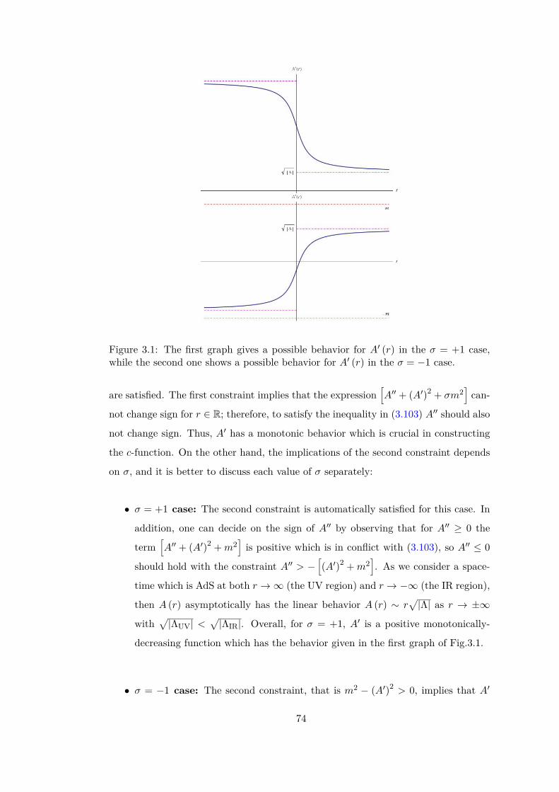
Figure 3.1: The first graph gives a possible behavior for A′ (r) in the σ = +1 case,while the second one shows a possible behavior for A′ (r) in the σ = −1 case.

are satisfied. The first constraint implies that the expression[A′′ + (A′)2 + σm2

]can-

not change sign for r ∈ R; therefore, to satisfy the inequality in (3.103) A′′ should also

not change sign. Thus, A′ has a monotonic behavior which is crucial in constructing

the c-function. On the other hand, the implications of the second constraint depends

on σ, and it is better to discuss each value of σ separately:

• σ = +1 case: The second constraint is automatically satisfied for this case. In

addition, one can decide on the sign of A′′ by observing that for A′′ ≥ 0 the

term[A′′ + (A′)2 +m2

]is positive which is in conflict with (3.103), so A′′ ≤ 0

should hold with the constraint A′′ > −[(A′)2 +m2

]. As we consider a space-

time which is AdS at both r →∞ (the UV region) and r → −∞ (the IR region),

then A (r) asymptotically has the linear behavior A (r) ∼ r√|Λ| as r → ±∞

with√|ΛUV| <

√|ΛIR|. Overall, for σ = +1, A′ is a positive monotonically-

decreasing function which has the behavior given in the first graph of Fig.3.1.

• σ = −1 case: The second constraint, that is m2 − (A′)2 > 0, implies that A′

74

is a bounded function as m > A′ > −m. Since A′ is monotonic and bounded,

A′′ should become zero as r → ±∞. In addition, to decide on the sign of A′′,

observe that for A′′ ≤ 0 the term[A′′ + (A′)2 −m2

]is negative due to the second

constraint and this result is in conflict with (3.103), so A′′ ≥ 0 should hold with

the bound A′′ < m2− (A′)2. We consider a spacetime which is AdS as r → ±∞

and due to the monotonically increasing nature of A′, an interesting possibility

appears: As r → +∞, A′ may attain a positive constant value and as r → −∞,

A′ may attain a negative constant value, so it is possible to have a spacetime

with two AdS “boundaries”. To sum up, for σ = −1, A′ is a monotonically

increasing function in the interval m > A′ > −m. A possible form for A′, which

yields a spacetime with two AdS boundaries, is given in the second graph of

Fig.3.1.

As a result, the null-energy condition implies that σA′′ ≤ 0; therefore, the c-function

for BINMG can be defined as

c (r) ≡ 3σ2G3A′ (r)

⇒ dc

dr≥ 0, (3.105)

which is the same as the c-function for Einstein’s gravity. As r → ∞, the value of

the c-function matches the central charge of the boundary CFT (3.24) and the Weyl

anomaly coefficient, which is discussed in the next section, up to a factor.

In addition to (3.105), one can define another c-function for BINMG, as the analysis

of (3.103) also implies the inequality

σA′′√m2 + σ (A′)2

≤ 0. (3.106)

The second c-function for BINMG can be defined as

c (r) ≡ −σ arctan

A′ (r)√m2 + σ (A′)2

, (3.107)

where the minus sign is introduced to make c (r) monotonically increasing function.

For σ = −1, the derivative of (3.107) directly gives the form in (3.106), while for

σ = +1, there is a positive factor of m2/[m2 + 2 (A′)2

]which does not effect the

inequality.13 To understand the relevance of this c-function, one needs to consider13 For σ = +1, one can define the c-function as c (r) = ln

[A′ +

√m2 + (A′)2

]by directly inte-

grating the form in (3.106). However, we prefer to give a single c-function for both values of σ.

75

the expansion of (3.106) in (A′/m)2. At the desired order, this expansion gives the

c-functions that were found in [22], but in the forms where the arbitrary coefficients

in [22] are fixed by the curvature expansion of BINMG.

3.4.2 Weyl anomaly

Now, by using holographic techniques let us calculate the Weyl anomaly14 for the

boundary CFT theory that is assumed to be dual of BINMG. As shown in [58], to

find the holographic Weyl anomaly, one needs to calculate the action of the bulk

gravity theory for the Einstein metric which induces a conformal structure on the

boundary and the logarithmic divergence that appears in this result yields the Weyl

anomaly for the boundary CFT. Furthermore, note that for a two-dimensional CFT

the Weyl anomaly coefficient a, which is defined by gµν 〈Tµν〉 = aR, and the central

charge of the Virasoro algebra are related as c = 24πa. Therefore, one can obtain the

c charge of the two-dimensional boundary CFT through a holographic calculation of

the Weyl anomaly from the three-dimensional bulk gravity theory.

To find the Weyl anomaly for BINMG, we follow [59] and calculate the BINMG action

for the Euclidean AdS3 metric

ds2 = dr2

1 + r2

`2

+ r2(dθ2 + sin2 θdφ2

), (3.108)

whose boundary is S2. This metric solves the field equations of BINMG, if `2 ≡ − 1λm2

satisfies (3.23). One can infer from (3.23) that AdS spacetime is possible if the bare

cosmological constant λ0 is in the interval 2 > λ0 > 0 for σ = −1 or λ0 < 0 for

σ = +1. Putting (3.108) in the BINMG action (3.99) yields

IBINMG = −16π`m2

κ2

[(1 + σ

`2m2

)3/2−(

1− λ02

)] ∫ r

0dr

r2√`2 + r2

, (3.109)

and after calculating the integral and using (3.22), one gets

IBINMG = 16π`m2λ0κ2

(1− λ0

4

)(1− λ0

2

)r2

2

×

√1 +(`

r

)2−(`

r

)2arcsinh

(r

`

) . (3.110)

14 For a nice review on Weyl anomaly, see [57].

76

Note that this result is valid for both values of σ as sign (λ0) = −σ. Here, we are

interested in the logarithmic term that appears in the asymptotic expansion of (3.110)

as r →∞ and it can be found as

4πσ`κ2 (2− λ0) ln

(2r`

), (3.111)

after using (3.23) and the expansion

√1 + x2 − x2arcsinh

(x−1

)= 1 + 1

2x2[1 + 2 ln

(x

2

)]+O

(x3). (3.112)

As discussed in [59], the coefficient of the logarithmic term is equal to c/3, so one

arrives at the same central charge result given in (3.24) which is obtained via the

method of equivalent quadratic curvature action.

77

CHAPTER 4

CONCLUSIONS

In this thesis, we developed the tools to analyze the unitarity of the D-dimensional

generic Born-Infeld (BI) gravity theory around the (A)dS background. In addition,

we studied a remarkable example of the Born-Infeld gravity theories which is the

Born-Infeld extension of new massive gravity (BINMG) in detail.

To analyze the unitarity of BI gravity theories around the (A)dS background, we

developed two general techniques. In constructing a modified gravity theory, the

absence of ghosts and tachyons in the spectrum is an important consistency criteria.

For BI gravity theories, checking this criteria around the flat background is rather

simple compared to the (A)dS background because only up to quadratic curvature

terms determine the flat space unitarity, while for the (A)dS space case all the terms

in the curvature expansion of the BI gravity effect the unitarity in principle. Thus,

constructing a unitary BI gravity theory around flat backgrounds is fairly easy and

there are examples starting with the original paper of Deser and Gibbons [8]. On the

other hand, without the techniques we developed such a construction is not possible for

the (A)dS background. In [6], using these techniques, the three-dimensional BINMG

theory is shown to be the first example of the unitary BI gravity theory around the

(A)dS background. Hopefully, these techniques enable one to construct further higher-

dimensional BI gravity theories around the (A)dS background.

The first of the techniques which can be applied to any BI gravity theory is based on

finding the O(h2) action which represents the free-theory of the excitations in the the-

ory. The O (h) and O(h2) actions for the generic BI gravity given in (2.18) and (2.21),

respectively, provide the required formulation to find the vacua and the spectrum for

78

a specific BI gravity once the O(h2) expansion of the A tensor is found. On the

other hand, the forms of O (h) and O(h2) actions for the generic BI gravity reveal the

remarkable fact that the even-dimensional BI gravity theory and its O(AD/2

)expan-

sion are equivalent with respect to vacua and spectrum. This equivalence may prove

to be useful in constructing an even dimensional unitary BI gravity theory around

the (A)dS background, since one needs to consider a finite order in curvature theory,

the O(AD/2

)expansion, instead of the original BI gravity which is infinite order in

curvature.

The second general technique is based on the construction of an equivalent quadratic

curvature action which have the same vacua and the same spectrum as the BI gravity.

The construction of the equivalent quadratic curvature action just involves calculat-

ing the Taylor series expansion in curvature for the Lagrangian around the, yet to

be found, (A)dS background. Differing form [5], the equivalent quadratic curvature

action is calculated from the original determinantal form of the BI action using the

formulation in (2.78–2.81) and in this way the technique becomes more streamlined.

When the two techniques are compared in application, the use of the O (h) and

O(h2) actions for the generic BI gravity is rather involved than finding the equiv-

alent quadratic curvature action because the metric perturbation, h, expansions of

the curvature tensors yield rather complicated expressions. In both of the techniques,

the final expressions are analyzed by using the existing unitarity discussions of the

generic quadratic curvature theories in [15].

To conclude, the techniques that we developed can be straightforwardly applied to

analyze unitarity of a specific BI gravity around the (A)dS background. Furthermore,

they are vital for a construction of a consistent BI gravity theory which is unitary

around the (A)dS background.

In considering BINMG, we discussed the construction of the theory in detail. Then,

using the techniques we developed, we demonstrated the unitarity of BINMG around

the (A)dS backgrounds. In addition, the Type-N and the Type-D solutions of BINMG

were found by using the Type-N and the Type-D solutions of TMG and NMG. Finally,

the two c-functions of BINMG were calculated.

79

REFERENCES

[1] K. S. Stelle, “Renormalization of Higher Derivative Quantum Gravity,” Phys.Rev. D 16, 953 (1977).

[2] K. S. Stelle, “Classical Gravity with Higher Derivatives,” Gen. Rel. Grav. 9, 353(1978).

[3] I. Gullu, T. C. Sisman, B. Tekin, “Born-Infeld extension of new massive gravity,”Class. Quant. Grav. 27, 162001 (2010).

[4] I. Gullu, T. C. Sisman and B. Tekin, “c-functions in the Born-Infeld extendedNew Massive Gravity,” Phys. Rev. D 82, 024032 (2010).

[5] I. Gullu, T. C. Sisman and B. Tekin, “Unitarity analysis of general Born-Infeldgravity theories,” Phys. Rev. D 82, 124023 (2010).

[6] I. Gullu, T. C. Sisman, B. Tekin, “All Bulk and Boundary Unitary Cubic Curva-ture Theories in Three Dimensions,” Phys. Rev. D 83, 024033 (2011).

[7] M. Gurses, T. C. Sisman and B. Tekin, “Some exact solutions of all f (Rµν)theories in three dimensions,” Phys. Rev. D 86, 024001 (2012).

[8] S. Deser and G. W. Gibbons, “Born-Infeld-Einstein actions?,” Class. Quant.Grav. 15, L35 (1998).

[9] M. Born and L. Infeld, “Foundations of the new field theory,” Proc. Roy. Soc.Lond. A 144, 425 (1934).

[10] A. Eddington, The Mathematical Theory of General Relativity (Cambridge Uni-versity Press, Cambridge, England, 1924).

[11] E. Bergshoeff, O. Hohm and P. K. Townsend, “Massive Gravity in Three Dimen-sions,” Phys. Rev. Lett., 102, 201301 (2009).

[12] E. Bergshoeff, O. Hohm and P. K. Townsend, “More on Massive 3D Gravity,”Phys. Rev. D 79, 124042 (2009).

[13] M. Nakasone and I. Oda, “On Unitarity of Massive Gravity in Three Dimen-sions,” Prog. Theor. Phys. 121, 1389 (2009).

[14] S. Deser, “Ghost-free, finite, fourth order D=3 (alas) gravity,” Phys. Rev. Lett.103, 101302 (2009).

[15] I. Gullu and B. Tekin, “Massive Higher Derivative Gravity in D-dimensionalAnti-de Sitter Spacetimes,” Phys. Rev. D 80, 064033 (2009).

[16] I. Gullu, T. C. Sisman and B. Tekin, “Canonical Structure of Higher DerivativeGravity in 3D,” Phys. Rev. D 81, 104017 (2010).

80

[17] K. Muneyuki and N. Ohta, “Unitarity versus Renormalizability of Higher Deriva-tive Gravity in 3D,” Phys. Rev. D 85, 101501 (2012).

[18] D. G. Boulware and S. Deser, “Can gravitation have a finite range?,” Phys. Rev.D 6, 3368 (1972).

[19] C. de Rham, G. Gabadadze, D. Pirtskhalava, A. J. Tolley and I. Yavin, “Nonlin-ear Dynamics of 3D Massive Gravity,” JHEP 1106, 028 (2011).

[20] M. F. Paulos and A. J. Tolley, “Massive Gravity Theories and limits of Ghost-freeBigravity models,” JHEP 1209, 002 (2012).

[21] I. Gullu, T. C. Sisman and B. Tekin, “Born-Infeld-Horava gravity,” Phys. Rev.D 81, 104018 (2010).

[22] A. Sinha, “On the new massive gravity and AdS/CFT,” JHEP 1006, 061 (2010).

[23] S. Nam, J. -D. Park, S. -H. Yi, “AdS Black Hole Solutions in the Extended NewMassive Gravity,” JHEP 1007, 058 (2010).

[24] M. Alishahiha, A. Naseh and H. Soltanpanahi, “On Born-Infeld Gravity in ThreeDimensions,” Phys. Rev. D 82, 024042 (2010).

[25] A. Ghodsi, D. M. Yekta, “Black Holes in Born-Infeld Extended New MassiveGravity,” Phys. Rev. D83, 104004 (2011).

[26] A. Ghodsi and D. M. Yekta, “On Asymptotically AdS-Like Solutions of ThreeDimensional Massive Gravity,” JHEP 1206, 131 (2012).

[27] H. Ahmedov and A. N. Aliev, “Type N Spacetimes as Solutions of Extended NewMassive Gravity,” Phys. Lett. B 711, 117 (2012).

[28] S. Dengiz and B. Tekin, “Higgs Mechanism for New Massive Gravity and WeylInvariant Extensions of Higher Derivative Theories,” Phys. Rev. D 84, 024033(2011).

[29] C. Senturk, T. C. Sisman and B. Tekin, “Energy and Angular Momentum inGeneric F(Riemann) Theories,” Phys. Rev. D 86, 124030 (2012).

[30] D. P. Jatkar and A. Sinha, “New Massive Gravity and AdS4 counterterms,” Phys.Rev. Lett. 106, 171601 (2011).

[31] S. Deser and B. Tekin, “Gravitational energy in quadratic curvature gravities,”Phys. Rev. Lett. 89, 101101 (2002).

[32] S. Deser and B. Tekin, “Energy in generic higher curvature gravity theories,”Phys. Rev. D 67, 084009 (2003).

[33] T. C. Sisman, I. Gullu and B. Tekin, “All unitary cubic curvature gravities in Ddimensions,” Class. Quant. Grav. 28, 195004 (2011) [arXiv:1103.2307 [hep-th]].

[34] P. Breitenlohner and D. Z. Freedman, “Positive Energy in anti-De Sitter Back-grounds and Gauged Extended Supergravity,” Phys. Lett. B 115, 197 (1982).

[35] A. Hindawi, B. A. Ovrut and D. Waldram, “Nontrivial vacua in higher derivativegravitation,” Phys. Rev. D 53, 5597 (1996).

81

[36] A. Higuchi, “Forbidden Mass Range For Spin-2 Field Theory In De Sitter Space-time,” Nucl. Phys. B 282, 397 (1987).

[37] P. Kraus and F. Larsen, “Microscopic black hole entropy in theories with higherderivatives,” JHEP 0509, 034 (2005).

[38] H. Saida and J. Soda, “Statistical entropy of BTZ black hole in higher curvaturegravity,” Phys. Lett. B 471, 358 (2000).

[39] C. Imbimbo, A. Schwimmer, S. Theisen and S. Yankielowicz, “Diffeomorphismsand holographic anomalies,” Class. Quant. Grav. 17, 1129 (2000).

[40] D. D. K. Chow, C. N. Pope and E. Sezgin, “Classification of solutions in topo-logically massive gravity,” Class. Quant. Grav. 27, 105001 (2010).

[41] M. Gurses, “Killing Vector Fields in Three Dimensions: A Method to Solve Mas-sive Gravity Field Equations,” Class. Quant. Grav. 27, 205018 (2010) [Erratum-ibid. 29, 059501 (2012)].

[42] H. Ahmedov and A. N. Aliev, “Exact Solutions in D-3 New Massive Gravity,”Phys. Rev. Lett. 106, 021301 (2011).

[43] H. Ahmedov and A. N. Aliev, “The General Type N Solution of New MassiveGravity,” Phys. Lett. B 694, 143 (2010).

[44] H. Ahmedov and A. N. Aliev, “Type D Solutions of 3D New Massive Gravity,”Phys. Rev. D 83, 084032 (2011).

[45] A. Garcia, F. W. Hehl, C. Heinicke, A. Macias, “The Cotton tensor in Rieman-nian space-times,” Class. Quant. Grav. 21, 1099-1118 (2004).

[46] S. Deser, R. Jackiw and S. Templeton, “Three-Dimensional Massive Gauge The-ories,” Phys. Rev. Lett. 48, 975 (1982).

[47] S. Deser, R. Jackiw and S. Templeton, “Topologically Massive Gauge Theories,”Annals Phys. 140, 372 (1982) [Erratum-ibid. 185, 406 (1988)] [Annals Phys. 281,409 (2000)].

[48] M. F. Paulos, “New massive gravity extended with an arbitrary number of curva-ture corrections,” Phys. Rev. D 82, 084042 (2010).

[49] Y. Nutku, “Exact solutions of topologically massive gravity with a cosmologicalconstant,” Class. Quant. Grav. 10, 2657 (1993).

[50] M. Gurses, “Perfect fluid sources in 2+1 dimensions,” Class. Quant. Grav. 11,2585 (1994).

[51] A. N. Aliev and Y. Nutku, “A theorem on topologically massive gravity,” Class.Quant. Grav. 13, L29 (1996).

[52] D. Z. Freedman, S. S. Gubser, K. Pilch and N. P. Warner, “Renormalization groupflows from holography supersymmetry and a c theorem,” Adv. Theor. Math. Phys.3, 363 (1999).

[53] L. Girardello, M. Petrini, M. Porrati and A. Zaffaroni, “The Supergravity dual ofN=1 superYang-Mills theory,” Nucl. Phys. B 569, 451 (2000).

82

[54] A. B. Zamolodchikov, “Irreversibility of the Flux of the Renormalization Groupin a 2D Field Theory,” JETP Lett. 43, 730, (1986).

[55] Z. Komargodski and A. Schwimmer, “On Renormalization Group Flows in FourDimensions,” JHEP 1112, 099 (2011).

[56] J. D. Brown and M. Henneaux, “Central Charges in the Canonical Realization ofAsymptotic Symmetries: An Example from Three-Dimensional Gravity,” Com-mun. Math. Phys. 104, 207 (1986).

[57] M. J. Duff, “Twenty years of the Weyl anomaly,” Class. Quant. Grav. 11, 1387(1994).

[58] M. Henningson and K. Skenderis, “The Holographic Weyl anomaly,” JHEP 9807,023 (1998).

[59] R. Emparan, C. V. Johnson and R. C. Myers, “Surface terms as counterterms inthe AdS / CFT correspondence,” Phys. Rev. D 60, 104001 (1999).

83

APPENDIX A

EXPANSIONS IN METRIC PERTURBATION

A.1 Second Order Expansions of Curvature Tensors

One of the approaches we use to analyze the spectrum of a BI gravity theory is to

calculate the second order action in metric perturbation. For such a calculation, the

second order expansions of curvature tensors are required and we derive them here.

The metric perturbation hµν is defined as

gµν ≡ gµν + τhµν , (A.1)

where gµν is the background metric and τ is introduced for bookkeeping purposes. In

considering expansions in hµν , one assumes that it is possible to find a coordinate frame

where components of hµν are small (in absolute value) compared to the components

of gµν . Surely, the (second order) expansions of curvature tensors in hµν have already

been considered in the literature, but here we derive the expansions relevant for us

and they are in the forms used in the subsequent calculations.

First, the second order expansion of the inverse metric can be found as

gµν = gµν − τhµν + τ2hµρhνρ +O(τ3). (A.2)

With this result, the Levi-Civita connection for gµν can be expanded up to second

order in hµν as

Γρµν = Γρµν + τ(Γρµν

)L− τ2hρβ

(Γβµν

)L

+O(τ3), (A.3)

where(Γρµν

)L

is the linearized Christoffel connection defined as

(Γρµν

)L≡ 1

2 gρλ(∇µhνλ + ∇νhµλ − ∇λhµν

), (A.4)

84

and Γρµν is the Levi-Civita connection for the background metric.

After finding the expansion for the Levi-Civita connection, we can derive our main

result, namely, the second order expansion of the Riemann tensor from which we find

the relevant expansions for the Ricci tensor and the scalar curvature. A variation in

the connection, that is δΓρµν = Γρµν − Γρµν , yields a variation in the Riemann tensor

Rµνρσ ≡ ∂ρΓµσν + ΓµρλΓλσν − ρ↔ σ as

Rµνρσ = Rµνρσ + ∇ρ (δΓµσν)− ∇σ(δΓµρν

)+ δΓµρλδΓ

λσν − δΓ

µσλδΓ

λρν , (A.5)

and for the second order expansion in hµν , the relevant δΓρµν is δΓρµν = τ(Γρµν

)L−

τ2hρβ

(Γβµν

)L

which yields

Rµνρσ =Rµνρσ + τ(Rµνρσ

)L− τ2hµβ

(Rβνρσ

)L

− τ2gµαgβγ[(

Γγρα)L

(Γβσν

)L− (Γγσα)L

(Γβρν

)L

]+O

(τ3). (A.6)

Here,(Rµνρσ

)L

is the linearized Riemann tensor with the definition

(Rµνρσ

)L≡ 1

2(∇ρ∇σhµν + ∇ρ∇νhµσ − ∇ρ∇µhσν

− ∇σ∇ρhµν − ∇σ∇νhµρ + ∇σ∇µhρν). (A.7)

Using (A.6), the second order expansions of the Ricci tensor and the scalar curvature

can be found as

Rνσ =Rνσ + τ (Rνσ)L − τ2hµβ

(Rβνµσ

)L

− τ2gµαgβγ[(

Γγµα)L

(Γβσν

)L− (Γγσα)L

(Γβµν

)L

]+O

(τ3), (A.8)

R =R+ τRL + τ2{Rρλhαρh

αλ − hνσ (Rνσ)L − g

νσhµβ

(Rβνµσ

)L

−gνσ gµαgβγ[(

Γγµα)L

(Γβσν

)L− (Γγσα)L

(Γβµν

)L

]}+O

(τ3),

(A.9)

where the linearized Ricci tensor RLνσ and the linearized curvature scalar RL are

defined as

RLνσ ≡12(∇µ∇σhµν + ∇µ∇νhµσ − �hσν − ∇σ∇νh

), (A.10)

RL = gαβRLαβ − Rαβhαβ. (A.11)

Here, h is the trace of hµν with the definition h ≡ gµνhµν . Note that the results

we obtained are valid for any background spacetime; however, in this thesis (A)dS

85

spacetimes are considered as the background spacetime when the second order action

for a BI gravity theory is studied.

A.2 Some linearization results in four dimensions

To linearize the field equations of the O[(αR)3

]expansion of BI gravity

I = 2κα

∫d4x

[√−det (gµν + αRµν)− (αΛ0 + 1)

√−g], (A.12)

one needs the following linearization results which are specific to four dimensions:

δ(RλναµR

λα)

= 2Λ3 RLµν + Λ

3 gµνRL + Λ2

3 hµν ,

δK = −2ΛRL, δS = 0,

δ (�Rµν) = �RLµν − Λ�hµν , δ (∇µ∇νR) = ∇µ∇νRL, δ (�R) = �RL,

δ(RρµRραR

αν

)= 3Λ2RLµν − 2Λ3hµν , δ

(RµνR

2αβ

)= 4Λ2RLµν + 2Λ2gµνRL, (A.13)

δ(RµνR

2)

= 16Λ2RLµν + 8Λ2gµνRL, δ (RRρνRµρ) = 8Λ2RLµν + Λ2gµνRL − 4Λ3hµν ,

δ (∇α∇µRαν ) = 12∇µ∇νRL + 4Λ

3 RLµν −Λ3 gµνRL −

4Λ2

3 hµν ,

δ (∇µ∇νRαβ) = ∇µ∇νRαβ − Λ∇µ∇νhαβ.

Some of these results were already given in [32], but they are reproduced here for

completeness. Note that the last two equations are related through the linearized

Bianchi identity:

∇µGLµν = 0, GLµν ≡ RLµν −12 gµνRL − Λhµν . (A.14)

A.3 Variations of cubic curvature terms

Variations of the cubic curvature terms RµνRρµRνρ , RRµνRνµ and R3 can be found as

δ(RµνR

ρµR

νρ

)= 3

[RρµRραR

αν + 1

2(gµνR

βρRαρ∇β∇α +RρνRµρ�− 2RρνRαρ∇µ∇α)]δgµν ,

(A.15)

δ(RRµνR

νµ

)=R

[(gµνR

αβ∇β∇α +Rµν�− 2Rαν∇µ∇α)

+ 2RρνRµρ]δgµν

+RαβRβα [(gµν�−∇µ∇ν) +Rµν ] δgµν , (A.16)

86

δ(R3)

= 3R2 [(gµν�−∇µ∇ν) +Rµν ] δgµν . (A.17)

The variation of Sαβ can be calculated by using

δRαβ = 12 (gµν∇α∇β + gµαgβν�− gβν∇µ∇α − gαν∇µ∇β) δgµν , (A.18)

δR = [Rµν + (gµν�−∇µ∇ν)] δgµν , (A.19)

as

δSαβ =12

[(gµν∇α∇β + gµαgβν�− gβν∇µ∇α − gαν∇µ∇β)− 2

3gαβ (gµν�−∇µ∇ν)]δgµν

+ 13

[(gµαgνβ −

13gαβgµν

)R− gαβSµν

]δgµν . (A.20)

Using this result, one can find δA ≡ δ(SαβS

βα

)and δB ≡ δ

(Sαρ S

βαS

ρβ

)as

δA =[2(SαµSαν + 1

3RSµν)

+(gµνS

αβ∇α∇β + Sµν�− 2Sαν∇µ∇α)]δgµν , (A.21)

δB =[3

2(gµνS

αρ S

βρ∇α∇β + SµρSρν�− 2Sαρ Sρν∇µ∇α

)− Sαρ Sρα (gµν�−∇µ∇ν)

]δgµν

+[3SρµSσρSνσ − Sαρ SραSµν +

(SµρS

ρν −

13gµνS

αρ S

ρα

)R

]δgµν . (A.22)

87

APPENDIX B

ANALYZING EINSTEIN’S GRAVITY AND

QUADRATIC CURVATURE GRAVITY WITH

SECOND ORDER PERTURBATIONS

In calculating the O(h2) action for a generic BI gravity theory, one encounters with

the O(h2) terms

∫d4x

√−g R(2),

∫d4x

√−g gµνR(2)

µν ,

∫d4x

√−g RµνL RLµν ,

∫d4x

√−g

(RµνρσR

ρσµν

)(2),

∫d4x

√−g gσν gλγ

(Rµρσλ

)(1) (Rρµγν

)(1), (B.1)

which should be written in terms of the building blocks that appear in Eqn. (25) of

[32]. To obtain the desired forms for these terms, we study them in the well-known

examples of Einstein’s gravity and quadratic curvature gravity.

B.1 Analysis of Einstein’s gravity

Expanding the cosmological Einstein-Hilbert action,

I = 1κ

∫d4x√−g (R− 2Λ0) , (B.2)

88

up to second order in metric perturbation hµν yields

I = 1κ

∫d4x

√−g

[1 + τ

2h+ 18τ

2(h2 − 2h2

µν

)+O

(τ3)]

×[(R− 2Λ0

)+ τRL + τ2R(2) +O

(τ3)]

= 1κ

∫d4x

√−g{(R− 2Λ0

)+ τ

[12h(R− 2Λ0

)+RL

]

+ τ2[1

8(R− 2Λ0

) (h2 − 2h2

µν

)+ 1

2hRL +R(2)

]+O

(τ3)}.

(B.3)

The first order term in this result can be used to find the field equations for the (A)dS

background. By using R = 4Λ and RL definition given in (A.11), the first order term

becomes

IO(h) = 1κ

∫d4x

√−g h (Λ− Λ0) , (B.4)

where a boundary term is dropped out. Then, after taking variation with respect to

hµν , the field equations for the (A)dS background follow as (Λ− Λ0) gµν = 0.

Now, let us consider the second order action which is

IO(h2) = 1κ

∫d4x

√−g

{hµν

[12

(Λ− 1

2Λ0

)(gµνh− 2hµν) + 1

2 gµνRL]

+R(2)

},

(B.5)

where R(2) is

R(2) =Rρλhαρhαλ − hµνRLµν − gνσhµβ

(Rβνµσ

)L

− gνσ gµαgβγ[(

Γγµα)L

(Γβσν

)L− (Γγσα)L

(Γβµν

)L

], (B.6)

from (A.9). To write∫d4x√−g R(2) in terms of the building blocks of [32], one should

work out the last three terms in R(2) by using the results in Appendix A.1 and the

maximally symmetric Riemann tensor form

Rµανβ = 2Λ(D − 1) (D − 2) (gµν gαβ − gµβ gαν) . (B.7)

The term gνσhµβ

(Rβνµσ

)L

can be written as

gνσhµβ

(Rβνµσ

)L

= hµν(RLµν −

4Λ3 hµν + Λ

3 gµνh), (B.8)

89

while the other two terms take the forms

∫d4x

√−g gνσ gµαgβγ

(Γγµα

)L

(Γβσν

)L

=∫d4x

√−g

[−1

2hµν(∇σ∇µhνσ + ∇σ∇νhµσ −

32∇µ∇νh

)+hµν

(4Λ3 hµν −

Λ12 gµνh

)+ 1

4hµν gµνRL

], (B.9)

∫d4x

√−g gνσ gµαgβγ (Γγσα)L

(Γβµν

)L

=∫d4x

√−g

[−1

4hµν(3�hµν − ∇σ∇µhσν − ∇σ∇νhµσ

)], (B.10)

after several integration by parts. Employing these results in∫d4x√−g R(2), finally,

one gets

∫d4x

√−g R(2) =

∫d4x

√−g hµν

(−1

2RLµν −

14 gµνRL + Λhµν −

Λ4 gµνh

). (B.11)

With this result, the O(h2) action for cosmological Einstein’s gravity (B.5) becomes

IO(h2) = − 12κ

∫d4x

√−g hµν

[GLµν + 1

2 (Λ0 − Λ) (gµνh− 2hµν)], (B.12)

and this result further reduces to the well-known form

IO(h2) = − 12κ

∫d4x

√−g hµνGLµν , (B.13)

after using the field equation for the (A)dS background, that is Λ = Λ0.

B.2 Analysis of quadratic curvature gravity

Now, let us study the most general quadratic curvature gravity in four dimensions;

I =∫d4x√−g

[1κ

(R− 2Λ0) + αR2 + βRµνRνµ

]. (B.14)

90

One can expand this action up to second order in hµν as

I =∫d4x

√−g

{[1κ

(R− 2Λ0

)+ αR2 + βRµν R

νµ

]+τ

[12h(1κ

(R− 2Λ0

)+ αR2 + βRµν R

νµ

)+(1κRL + 2αRRL + βRµνRLµν + β (Rµν)(1) Rµν

)](B.15)

+τ2[1

8(h2 − 2h2

µν

)(1κ

(R− 2Λ0

)+ αR2 + βRµν R

νµ

)+1

2h(1κRL + 2αRRL + βRµνRLµν + β (Rµν)(1) Rµν

)+(1κR(2) + 2αRR(2) + αR2

L + βRµνR(2)µν + β (Rµν)(1)R

Lµν + β (Rµν)(2) Rµν

)]},

where (Rµν)(1) and (Rµν)(2) represent the first and the second orders of Rµν in metric

perturbation, respectively. From the linear order of this expansion, one should first

find the field equation for the (A)dS background. By using the definitions of RLµν and

RL, the linear order terms take the form

IO(h) = 1κ

∫d4x

√−g h (Λ− Λ0) , (B.16)

after dropping out the boundary terms, and one can directly read the field equation

as Λ = Λ0.

Now, let us consider the O(h2) action which takes the form

IO(h2) = −12

∫d4x

√−g

{(1κ

+ 8αΛ + 4βΛ)hµνGLµν

−12h

2[1κ

(Λ− Λ0) + 2βΛ2]

(B.17)

+h2µν

[1κ

(Λ− Λ0) + 6βΛ2]

+2αhµν(gµν�− ∇µ∇ν + Λgµν

)RL

−2β(ΛgµνR(2)

µν +RµνL RLµν +Rµν(2)Λgµν)}

,

after using (B.11). We should rewrite the three terms in the last line in terms of the

building blocks of [32]. First, the term∫d4x√−g RµνL RLµν can be put in the desired

form as∫d4x

√−g RµνL RLµν = −1

2

∫d4x

√−g hµν

[(gµν�− ∇µ∇ν + Λgµν

)RL

+(�GLµν −

2Λ3 gµνRL

)−14Λ

3 RLµν + Λ3 gµνRL + 8Λ2

3 hµν

], (B.18)

91

after several integration by parts and using the linearized Bianchi identity;

∇µGLµν = 0, GLµν ≡ RLµν −12 gµνRL − Λhµν , (B.19)

and its variant;

∇µ∇νRLµν = 12�RL + Λ∇µ∇νhµν . (B.20)

Turning to the other two terms, note that the term gµν (Rµν)(2) is simply related to

gµνR(2)µν as

gµν (Rµν)(2) = gµν(gµαgνβRαβ

)(2)= gµνR(2)

µν − 2hµνRLµν + 3Λh2µν , (B.21)

and the term gµνR(2)µν can be written in terms of R(2) as

R(2) = (gµνRµν)(2) = gµνR(2)µν − hµνRLµν + Λh2

µν . (B.22)

By using this result and (B.11),∫d4x√−g gµνR(2)

µν takes the form

∫d4x

√−g gµνR(2)

µν =∫d4x

√−g hµν

(12R

Lµν −

14 gµνRL −

Λ4 gµνh

). (B.23)

By using (B.18), (B.21), (B.23), and the field equation for the (A)dS background, the

second order action for the most general quadratic curvature gravity in four dimensions

becomes

IO(h2) = −12

∫d4x

√−g hµν

[(1κ

+ 8αΛ + 43βΛ

)GLµν

+ (2α+ β)(gµν�− ∇µ∇ν + Λgµν

)RL

+β(�GLµν −

2Λ3 gµνRL

)], (B.24)

which matches the form given in [32].

Now, let us study the Einstein-Gauss-Bonnet theory,

I =∫d4x√−g

[1κ

(R− 2Λ0) + γ(RµνρσR

ρσµν − 4RµνRνµ +R2

)], (B.25)

to work out the terms in the second line of (B.1). Note that Gauss-Bonnet combination

is a boundary term in four dimensions, so the field equation for the (A)dS background

and the O(h2) action should the same as the corresponding results in the Einstein’s

gravity case.

92

The O(h2) action for the terms other than RµνρσR

ρσµν can be given as

IO(h2) = −12

∫d4x

√−g hµν

[(1κ

+ 83γΛ

)GLµν − 2γ

(gµν�− ∇µ∇ν + Λgµν

)RL

− 4γ(�GLµν −

2Λ3 gµνRL

)], (B.26)

by using (B.24). On the other hand, to find the O(h2) action for RµνρσRρσµν , let us

expand it up to O(h2) as

I = γ

∫d4x

√−g{RµνρσR

ρσµν + τ

[(RµνρσR

ρσµν

)(1)+ 1

2hRµνρσR

ρσµν

]

+ τ2[(RµνρσR

ρσµν

)(2)+ 1

2h(RµνρσR

ρσµν

)(1)+ 1

8RµνρσR

ρσµν

(h2 − 2h2

µν

)]}.

(B.27)

One expects that the linear order of this expansion should become a boundary term

in order not to effect the field equation for the (A)dS background. One can calculate

that

RµνρσRρσµν = 8Λ2

3 ,(RµνρσR

ρσµν

)(1)= 4Λ

3 RL, (B.28)

then the linear order of (B.27) becomes

IO(h) =∫d4x

√−g

[(∇µ∇νhµν − �h

)], (B.29)

which is a boundary term.

Now, let us study the O(h2) of (B.27) which becomes

IO(h2) = γ

∫d4x

√−g

[(RµνρσR

ρσµν

)(2)+ 2Λ

3 hRL + Λ2

3(h2 − 2h2

µν

)], (B.30)

after using (B.28). Here,(RµνρσR

ρσµν

)(2)can be written as(

RµνρσRρσµν

)(2)=(RµρσλR

ρµγνg

σνgλγ)(2)

=2Rρ λσµ

(Rµρσλ

)(2)+ 2RµρσλR

ρ λµ νg

σν(2) + gσν gλγ

(Rµρσλ

)(1) (Rρµγν

)(1)

+ 2[Rρ λ

µ ν

(Rµρσλ

)(1)+ Rµ γ

ρσ

(Rρµγν

)(1)]gσν(1) + RµρσλR

ρµγνg

σν(1)g

λγ(1),

(B.31)

and by employing (B.7), (B.8), and R(2) = gρσR(2)ρσ + gρσ(1)R

(1)ρσ + Rρσg

ρσ(2), it further

reduces to (RµνρσR

ρσµν

)(2)=4Λ

3 R(2) − gσν gλγ(Rµρλσ

)(1) (Rρµγν

)(1)

− 4Λ3 hµνRLµν + 14Λ2

9 h2µν −

2Λ2

9 h2. (B.32)

93

Let us consider the integral of this form where the second term can be calculated as

∫d4x

√−g gµν gρα

(Rλσρµ

)(1)(Rσλαν)(1)

=∫d4x

√−g{hµν

[2(�GLµν −

2Λ3 gµνRL

)+(gµν�− ∇µ∇ν + Λgµν

)RL

]

− Λ9 h

µν(30RLµν − 9gµνRL − 32Λhµν + 2Λgµνh

)}, (B.33)

after a rather lengthy but straightforward computation involving several integration

by parts. Putting this result and (B.11) in∫d4x√−g

(RµνρσR

ρσµν

)(2), one finally gets

∫d4x

√−g

(RµνρσR

ρσµν

)(2)=∫

d4x√−g hµν

{−[2(�GLµν −

2Λ3 gµνRL

)+(gµν�− ∇µ∇ν + Λgµν

)RL

]

+ Λ3(8GLµν − 4RLµν + 6Λhµν − Λgµνh

)}. (B.34)

Now, we are ready to write the O(h2) of I = γ

∫d4x√−g RµνρσRρσµν which becomes

IO(h2) = −12γ∫d4x

√−g hµν[

−8Λ3 G

Lµν + 2

(gµν�− ∇µ∇ν + Λgµν

)RL + 4

(�GLµν −

2Λ3 gµνRL

)].

(B.35)

One can obtain the O(h2) of the Einstein-Gauss-Bonnet theory by adding this result

and (B.26), and in the final form there is not any contribution coming from the Gauss-

Bonnet term as expected.

94

CURRICULUM VITAE

Personal Information

Surname, Name: Sisman, Tahsin Cagrı

Nationality: Turkish

Date and Place of Birth: 09 August 1980, Kayseri

Phone: +90 543 476 27 91

Email: tahsin.c.sisman@gmail.com

Education

• Ph. D. in Physics, (September 2005 – September 2012),

Middle East Technical University,

Advisor: Prof. Dr. Bayram Tekin,

Thesis: Born-Infeld gravity theories in D-dimensions.

• M. Sc. in Mechanical Engineering, (October 2002 – September 2005),

Middle East Technical University,

Advisor: Prof. Dr. M. Haluk Aksel,

Thesis: Parallel processing of three-dimensional Navier-Stokes equations for

compressible flows.

• B. Sc. in Physics, (September 2000 – January 2004),

Middle East Technical University.

• B. Sc. in Mechanical Engineering, (September 1998 – June 2002),

Middle East Technical University.

95

Employment and Experience

• Researcher in the project “Classical and Quantum Mechanical Structure of

Higher Derivative Gravity Theories in 2+1 Dimensions” supported by The Scien-

tific and Technological Research Council of Turkey under the grant No. 110T339,

November 2010 – November 2012.

• Teaching assistant in the Mechanical Engineering Department of Middle East

Technical University, November 2002 – September 2005.

Honors and Awards

• Bruno Ferretti Diploma at International School of Subnuclear Physics, Erice,

Italy, 2011.

• Scholarship for PhD study from The Scientific and Technological Research Coun-

cil of Turkey, March 2006 – August 2010.

• Second place in Physics National Project Competition between high school stu-

dents organized by The Scientific and Technological Research Council of Turkey,

1997.

Publications

1. C. Senturk, T. C. Sisman and B. Tekin, “Energy and Angular Momentum in

Generic F(Riemann) Theories,” Phys. Rev. D 86, 124030 (2012) [arXiv:1209.2056

[hep-th]].

2. T. C. Sisman, I. Gullu and B. Tekin, “Spectra, vacua, and the unitarity of

Lovelock gravity in D-dimensional AdS spacetimes,” ’ Phys. Rev. D 86, 044041

(2012) [arXiv:1204.3814 [hep-th]].

3. M. Gurses, T. C. Sisman and B. Tekin, “New Exact Solutions of Quadratic

Curvature Gravity,” Phys. Rev. D 86, 024009 (2012) [arXiv:1204.2215 [hep-th]].

96

4. M. Gurses, T. C. Sisman and B. Tekin, “Some exact solutions of all f(Ricci)

theories in three dimensions,” Phys. Rev. D 86, 024001 (2012) [arXiv:1112.6346

[hep-th]].

5. T. C. Sisman, I. Gullu and B. Tekin, “All unitary cubic curvature gravities in D

dimensions,” Class. Quant. Grav. 28, 195004 (2011) [arXiv:1103.2307 [hep-th]].

6. I. Gullu, M. Gurses, T. C. Sisman and B. Tekin, “AdS Waves as Exact Solutions

to Quadratic Gravity,” Phys. Rev. D 83, 084015 (2011) [arXiv:1102.1921 [hep-

th]].

7. S. Deser, H. Liu, H. Lu, C. N. Pope, T. C. Sisman and B. Tekin, “Critical

Points of D-Dimensional Extended Gravities,” Phys. Rev. D 83, 061502(R)

(2011) [arXiv:1101.4009 [hep-th]].

8. I. Gullu, T. C. Sisman and B. Tekin, “All Bulk and Boundary Unitary Cubic

Curvature Theories in Three Dimensions,” Phys. Rev. D 83, 024033 (2011)

[arXiv:1011.2419 [hep-th]].

9. I. Gullu, T. C. Sisman and B. Tekin, “Unitarity analysis of general Born-Infeld

gravity theories,” Phys. Rev. D 82, 124023 (2010) [arXiv:1010.2411 [hep-th]].

10. I. Gullu, T. C. Sisman and B. Tekin, “c-functions in the Born-Infeld extended

New Massive Gravity,” Phys. Rev. D 82, 024032 (2010) [arXiv:1005.3214 [hep-

th]].

11. I. Gullu, T. C. Sisman and B. Tekin, “Born-Infeld-Horava gravity,” Phys. Rev.

D 81, 104018 (2010) [arXiv:1004.0611 [hep-th]].

12. I. Gullu, T. C. Sisman and B. Tekin, “Born-Infeld extension of new massive

gravity,” Class. Quant. Grav. 27, 162001 (2010) [arXiv:1003.3935 [hep-th]].

13. I. Gullu, T. C. Sisman and B. Tekin, “Canonical Structure of Higher Derivative

Gravity in 3D,” Phys. Rev. D 81, 104017 (2010) [arXiv:1002.3778 [hep-th]].

14. T. C. Sisman and B. Tekin, “Green’s Matrix for a Second Order Self-Adjoint

Matrix Differential Operator,” J. Phys. A 43, 125205 (2010) [arXiv:0908.0223

[math-ph]].

97

Presentations

• Title of the talk: Critical gravity in D-dimensions,

– “Sixth Aegean Summer School - Quantum Gravity and Quantum Cosmol-

ogy,” Chora, Greece, September 16, 2011;

– “International School of Subnuclear Physics,” Erice, Italy, June 25, 2011;

– “SIGRAV Graduate School - IX Edition Analogue Gravity,” Como, Italy,

May 21, 2011;

– “Applied Mathematics Group: Thursday Seminars,” Department of Math-

ematics, Bilkent University, Ankara, Turkey, January 27, 2011.

• Title of the talk: Unitarity analysis of general Born-Infeld gravity theories,

– “10th Workshop on Quantization, Dualities and Integrable Systems,” Ma-

gusa, Turkish Republic of Northern Cyprus, April 22, 2011;

– “Applied Mathematics Group: Thursday Seminars,” Department of Math-

ematics, Bilkent University, Ankara, Turkey, October 21, 2010.

• Title of the talk: New Massive Gravity in de-Sitter Space and Chiral Gravity,

– “9th Workshop on Quantization, Dualities and Integrable Systems,” Istan-

bul, Turkey, April 24, 2010.

• Title of the talk: Quantum Corrections to the Instantons in the Two Dimen-

sional Abelian Higgs Model: Functional Determinants and Green’s Function

Techniques,

– “8th Workshop on Quantization, Dualities and Integrable Systems,” Ankara,

Turkey, April 23, 2009.

Conferences, Workshops, Schools

• Workshop on Infrared Modifications of Gravity, The Abdus Salam International

Centre for Theoretical Physics, Trieste, Italy, September 26–30, 2011.

• Sixth Aegean Summer School - Quantum Gravity and Quantum Cosmology,

Chora, Naxos, Greece, September 12–17, 2011.

98

• Istanbul 2011: Strings, Branes and Supergravity, Koc University, Istanbul, Turkey,

August 01–05, 2011.

• International School of Subnuclear Physics (49th Course) - Searching for the

Unexpected at LHC and Status of Our Knowledge, Ettore Majorana Foundation

and Centre for Scientific Culture, Erice, Italy, June 24 – July 03, 2011.

• ICTP Summer School on Particle Physics, The Abdus Salam International Cen-

tre for Theoretical Physics, Trieste, Italy, June 06–17, 2011.

• SIGRAV Graduate School in Contemporary Relativity and Gravitational Physics

- IX Edition Analogue Gravity, Centro di Cultura Scientifica ”Alessandro Volta”,

Villa Olmo, Como, Italy, May 16–21, 2011.

• 10th Workshop on Quantization, Dualities and Integrable Systems, Eastern Mediter-

ranean University, Magusa, Turkish Republic of Northern Cyprus, April 22–24,

2011.

• 9th Workshop on Quantization, Dualities and Integrable Systems, Yeditepe Uni-

versity, Istanbul, Turkey, April 23–25, 2010.

• Lectures on Neutrino Mass and Grand Unified Theories, Feza Gursey Institute

for Fundamental Sciences, Istanbul, Turkey, July 27 – August 01, 2009.

• 8th Workshop on Quantization, Dualities and Integrable Systems, Ankara Uni-

versity, Ankara, Turkey, April 23–25, 2009.

• A Short Course on Supergravity, Istanbul Center for Mathematical Sciences,

Turkey, February 05–06, 2009.

• Lie Groups and Representation Theory, Feza Gursey Institute for Fundamental

Sciences, Istanbul, Turkey, July 28 – August 08, 2008.

• Phase Transitions and Renormalization Group, Feza Gursey Institute for Fun-

damental Sciences, Istanbul, Turkey, July 13–24, 2008.

• Rigorous Results in Statistical Mechanics and Quantum Field Theory, Feza

Gursey Institute for Fundamental Sciences, Istanbul, Turkey, June 12–20, 2008.

99

• 7th Workshop on Quantization, Dualities and Integrable Systems, Anadolu Uni-

versity, Eskisehir, Turkey, April 23–25, 2008.

• High Energy Physics School, Feza Gursey Institute for Fundamental Sciences,

Istanbul, Turkey, June 25 – August 03, 2007.

• 6th Workshop on Quantization, Dualities and Integrable Systems, Middle East

Technical University, Ankara, Turkey, April 20–22, 2007.

100