“Bootstrapping” students’ understanding of statistical ... report.pdf · to develop students’ understanding of statistical inference concepts and ... some common pre-test

“Bootstrapping” students’ understanding of statistical inference

Maxine Pfannkuch, Sharleen Forbes, John Harraway, Stephanie Budgett and Chris Wild

April 2013

SuMMAry 2“BootStrAPPing” StudentS’ underStAnding oF StAtiStiCAl inFerenCe

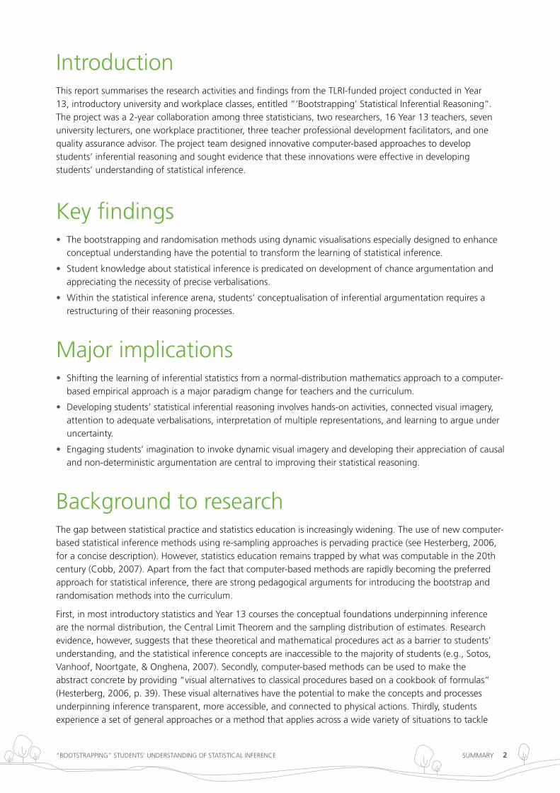
introductionthis report summarises the research activities and findings from the tlri-funded project conducted in year 13, introductory university and workplace classes, entitled “‘Bootstrapping’ Statistical inferential reasoning”. the project was a 2-year collaboration among three statisticians, two researchers, 16 year 13 teachers, seven university lecturers, one workplace practitioner, three teacher professional development facilitators, and one quality assurance advisor. the project team designed innovative computer-based approaches to develop students’ inferential reasoning and sought evidence that these innovations were effective in developing students’ understanding of statistical inference.

Key findingsthe bootstrapping and randomisation methods using dynamic visualisations especially designed to enhance •conceptual understanding have the potential to transform the learning of statistical inference.

Student knowledge about statistical inference is predicated on development of chance argumentation and •appreciating the necessity of precise verbalisations.

Within the statistical inference arena, students’ conceptualisation of inferential argumentation requires a •restructuring of their reasoning processes.

Major implicationsShifting the learning of inferential statistics from a normal-distribution mathematics approach to a computer-•based empirical approach is a major paradigm change for teachers and the curriculum.

developing students’ statistical inferential reasoning involves hands-on activities, connected visual imagery, •attention to adequate verbalisations, interpretation of multiple representations, and learning to argue under uncertainty.

engaging students’ imagination to invoke dynamic visual imagery and developing their appreciation of causal •and non-deterministic argumentation are central to improving their statistical reasoning.

Background to research the gap between statistical practice and statistics education is increasingly widening. the use of new computer-based statistical inference methods using re-sampling approaches is pervading practice (see Hesterberg, 2006, for a concise description). However, statistics education remains trapped by what was computable in the 20th century (Cobb, 2007). Apart from the fact that computer-based methods are rapidly becoming the preferred approach for statistical inference, there are strong pedagogical arguments for introducing the bootstrap and randomisation methods into the curriculum.

First, in most introductory statistics and year 13 courses the conceptual foundations underpinning inference are the normal distribution, the Central limit theorem and the sampling distribution of estimates. research evidence, however, suggests that these theoretical and mathematical procedures act as a barrier to students’ understanding, and the statistical inference concepts are inaccessible to the majority of students (e.g., Sotos, Vanhoof, noortgate, & onghena, 2007). Secondly, computer-based methods can be used to make the abstract concrete by providing “visual alternatives to classical procedures based on a cookbook of formulas” (Hesterberg, 2006, p. 39). these visual alternatives have the potential to make the concepts and processes underpinning inference transparent, more accessible, and connected to physical actions. thirdly, students experience a set of general approaches or a method that applies across a wide variety of situations to tackle


problems rather than learning multiple and separate formulas for each situation (Wood, 2005). Moreover, these methods, coupled with dynamic visualisation infrastructure, allow access to statistical concepts previously considered too advanced for students, as mastery of algebraic representations is not a prerequisite. As Wood (2005, p. 9) states, simulation approaches such as the bootstrap “offer the promise of liberating statistics from the shackles of the symbolic arguments that many people find so difficult”.

even though many statisticians have been calling for reform in statistics education, it is only recently that computer-intensive methods are being established in introductory courses using mainly a randomisation-based curriculum and commercial software (garfield, delMas, & Zieffler, 2012; gould, davis, Patel, & esfandiari, 2010; Holcomb, Chance, rossman, tietjen, & Cobb, 2010; tintle, topliff, Vanderstoep, Holmes, & Swanson, 2012; tintle, Vanderstoep, Holmes, Quisenberry, & Swanson, 2011). in new Zealand, we are taking a different approach, using bootstrapping for sample-to-population inference and the randomisation test for experiment-to-causal inference and developing purpose-built software to facilitate student access to inferential concepts. this current project also builds on the findings and learning progressions developed for years 10 to 12 (Pfannkuch, Arnold, & Wild, 2011; Pfannkuch & Wild, 2012). Since our proposals for teaching statistical inference are new for year 13, introductory university, and workplace students, questions arise about how to develop students’ understanding of statistical inference concepts and their reasoning processes. these questions were particularly important, as the new year 13 curriculum requires students to use and understand these new statistical practice methods of bootstrapping and randomisation for inference.

Methodologythe methodology employed in this study is design research. in cognisance of learning theories (e.g., Clark & Paivio, 1991), this research designs learning trajectories that engineer new types of statistical inferential reasoning and then revises them in the light of evidence about student learning and reasoning. design research aims to develop theories about learning and instructional design as well as to improve learning and provide practitioners with accessible results and learning materials (Bakker, 2004). using Hjalmarson and lesh’s (2008) design research principles, the development process in this project involved two research cycles with four phases: (1) the understanding and defining of the conceptual foundations of inference, (2) development of learning trajectories, new resource materials, and dynamic visualisation software, (3) implementation with students, and (4) retrospective analysis followed by modification of teaching materials.

the research was conducted over 2 years and went through two developmental cycles. in the first year, there was a pilot study involving five year 13 and five university students while in the second year, the main study involved 2765 students from throughout new Zealand (14 year 13 classes, seven introductory university classes, one workplace class). the main data collected were pre- and post-tests of all the students, pre- and post-interviews with 38 students, task-interviews with 12 students, videos of three classes implementing the learning trajectories, and teacher and lecturer reflections. note there were two versions of the post-test in the main study to which students were randomly allocated. time constraints meant that there was a bootstrapping post-test and a randomisation post-test with some common pre-test items.

AnalysisFor the pre- and post-tests, assessment frameworks were developed from the student data for 11 free-response questions. two independent people coded the free-response questions and then came to a consensus on the final codes. Statistical analyses using r and inZight software were conducted on the coded data as well as the multi-choice items. nVivo was used to qualitatively analyse the interview data (Braun & Clark, 2006).


resultsresearch Question 1: What learning trajectories will facilitate students’ conceptual access to the ideas behind statistical inference using bootstrapping and randomisation methods?

to answer this question we first explicitly extracted the conceptual foundations underpinning statistical inference argumentation. Secondly, we created the desired dynamic visual imagery software for revealing the processes behind the new inferential methods (see http://www.stat.auckland.ac.nz/~wild/Vit/). thirdly, we developed new verbalisations for describing the processes and representational infrastructure in the software that we had created. Since current statistical language was also insufficient to describe the conceptual and argumentation ideas that we had uncovered, we developed further verbalisations in order to facilitate students’ conceptual access to statistical inference (see Pfannkuch, regan, Wild, Budgett, Forbes, Harraway, & Parsonage, 2011, for discussion on some of the language issues). Fourthly, we designed and trialled learning trajectories. the main principles behind the instruction were that:

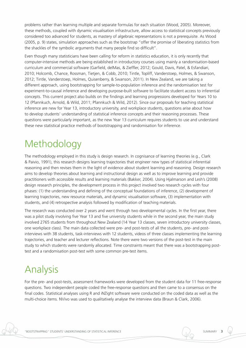
learning trajectories should have hands-on simulation activities before moving to computer environments •(see Figure 1)

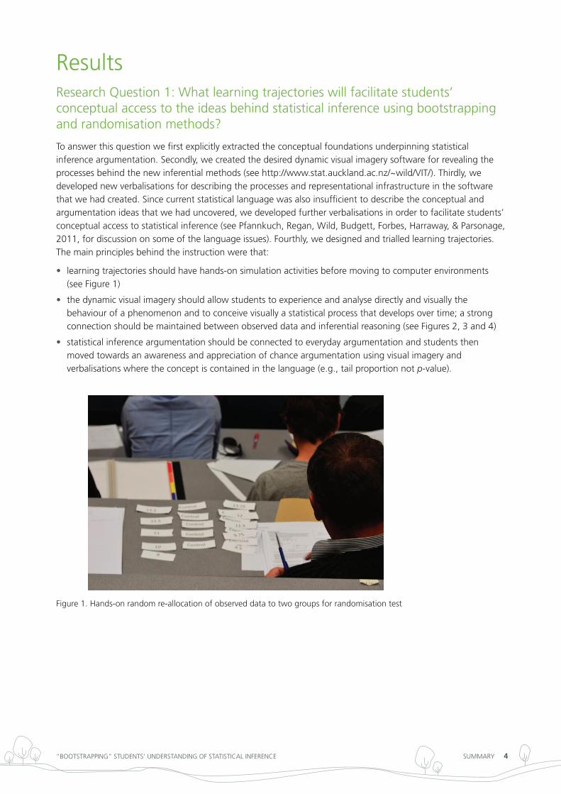
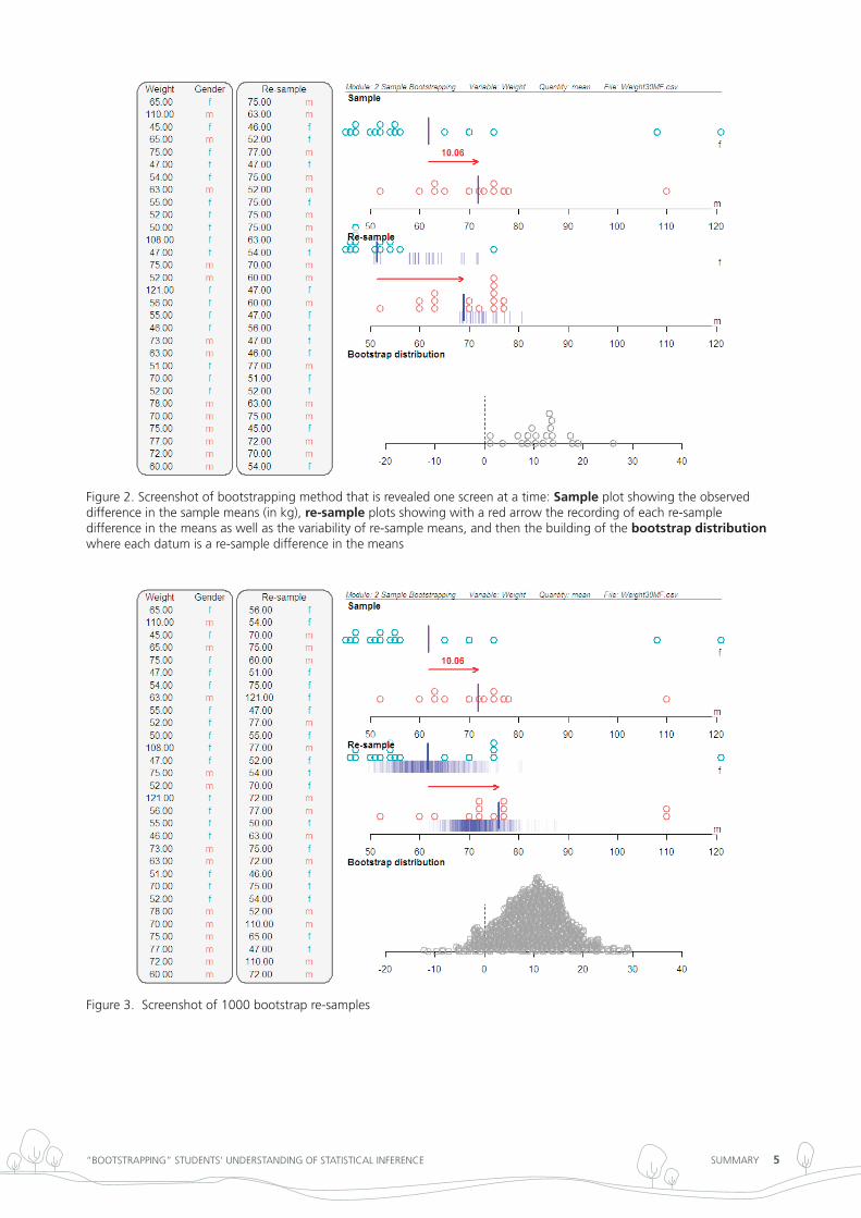
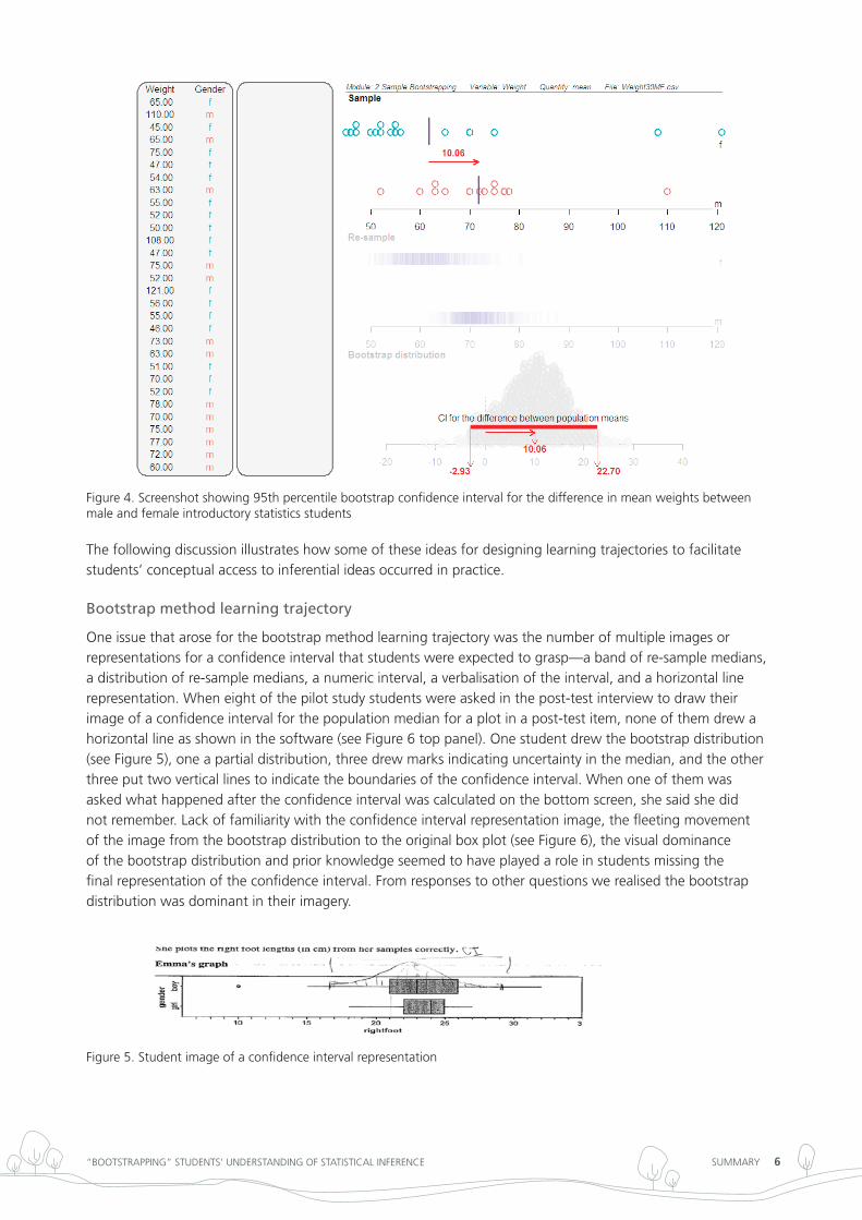
the dynamic visual imagery should allow students to experience and analyse directly and visually the •behaviour of a phenomenon and to conceive visually a statistical process that develops over time; a strong connection should be maintained between observed data and inferential reasoning (see Figures 2, 3 and 4)

statistical inference argumentation should be connected to everyday argumentation and students then •moved towards an awareness and appreciation of chance argumentation using visual imagery and verbalisations where the concept is contained in the language (e.g., tail proportion not p-value).

Figure 1. Hands-on random re-allocation of observed data to two groups for randomisation test


Figure 2. Screenshot of bootstrapping method that is revealed one screen at a time: Sample plot showing the observed difference in the sample means (in kg), re-sample plots showing with a red arrow the recording of each re-sample difference in the means as well as the variability of re-sample means, and then the building of the bootstrap distribution where each datum is a re-sample difference in the means

Figure 3. Screenshot of 1000 bootstrap re-samples


Figure 4. Screenshot showing 95th percentile bootstrap confidence interval for the difference in mean weights between male and female introductory statistics students

the following discussion illustrates how some of these ideas for designing learning trajectories to facilitate students’ conceptual access to inferential ideas occurred in practice.

Bootstrap method learning trajectory

one issue that arose for the bootstrap method learning trajectory was the number of multiple images or representations for a confidence interval that students were expected to grasp—a band of re-sample medians, a distribution of re-sample medians, a numeric interval, a verbalisation of the interval, and a horizontal line representation. When eight of the pilot study students were asked in the post-test interview to draw their image of a confidence interval for the population median for a plot in a post-test item, none of them drew a horizontal line as shown in the software (see Figure 6 top panel). one student drew the bootstrap distribution (see Figure 5), one a partial distribution, three drew marks indicating uncertainty in the median, and the other three put two vertical lines to indicate the boundaries of the confidence interval. When one of them was asked what happened after the confidence interval was calculated on the bottom screen, she said she did not remember. lack of familiarity with the confidence interval representation image, the fleeting movement of the image from the bootstrap distribution to the original box plot (see Figure 6), the visual dominance of the bootstrap distribution and prior knowledge seemed to have played a role in students missing the final representation of the confidence interval. From responses to other questions we realised the bootstrap distribution was dominant in their imagery.

Figure 5. Student image of a confidence interval representation


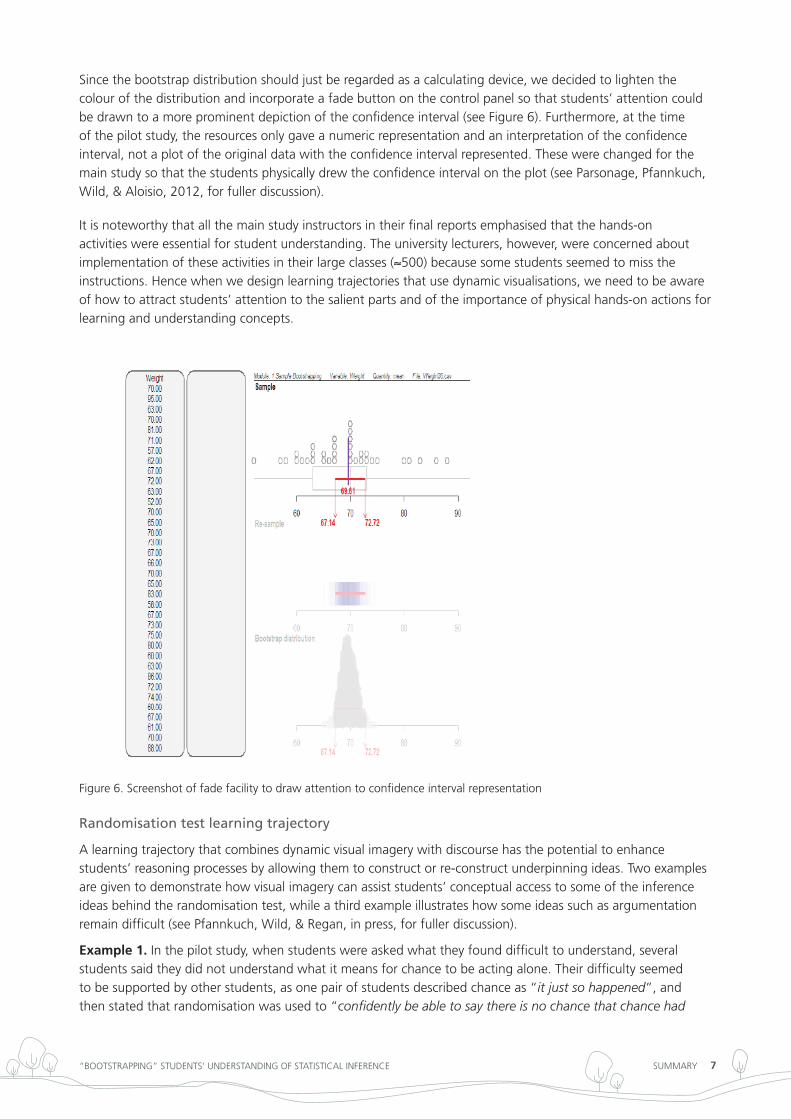
Since the bootstrap distribution should just be regarded as a calculating device, we decided to lighten the colour of the distribution and incorporate a fade button on the control panel so that students’ attention could be drawn to a more prominent depiction of the confidence interval (see Figure 6). Furthermore, at the time of the pilot study, the resources only gave a numeric representation and an interpretation of the confidence interval, not a plot of the original data with the confidence interval represented. these were changed for the main study so that the students physically drew the confidence interval on the plot (see Parsonage, Pfannkuch, Wild, & Aloisio, 2012, for fuller discussion).

it is noteworthy that all the main study instructors in their final reports emphasised that the hands-on activities were essential for student understanding. the university lecturers, however, were concerned about implementation of these activities in their large classes (≈500) because some students seemed to miss the instructions. Hence when we design learning trajectories that use dynamic visualisations, we need to be aware of how to attract students’ attention to the salient parts and of the importance of physical hands-on actions for learning and understanding concepts.

Figure 6. Screenshot of fade facility to draw attention to confidence interval representation

Randomisation test learning trajectory

A learning trajectory that combines dynamic visual imagery with discourse has the potential to enhance students’ reasoning processes by allowing them to construct or re-construct underpinning ideas. two examples are given to demonstrate how visual imagery can assist students’ conceptual access to some of the inference ideas behind the randomisation test, while a third example illustrates how some ideas such as argumentation remain difficult (see Pfannkuch, Wild, & regan, in press, for fuller discussion).

Example 1. in the pilot study, when students were asked what they found difficult to understand, several students said they did not understand what it means for chance to be acting alone. their difficulty seemed to be supported by other students, as one pair of students described chance as “it just so happened”, and then stated that randomisation was used to “confidently be able to say there is no chance that chance had


any effect on the results”. When questioned on the hands-on activities that formed part of the randomisation teaching sequence (see Figure 1), another pair of students understood the ticket-tearing procedure as “creating chance”. Since the idea that chance is acting alone is a central concept in the randomisation method, we were concerned about the students’ difficulties with this notion. Consequently new software, designed to visually illustrate chance is acting alone, unencumbered by experimental data, was developed.

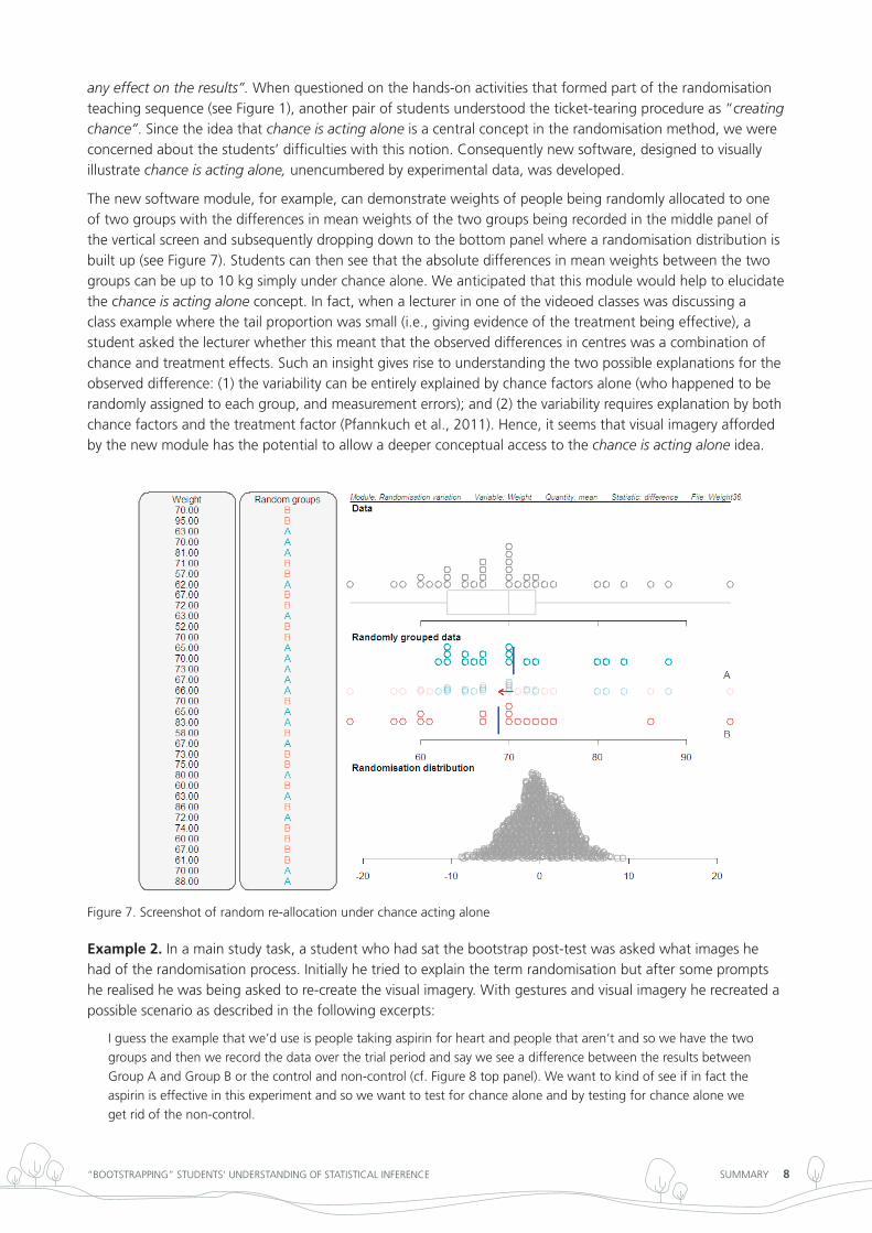
the new software module, for example, can demonstrate weights of people being randomly allocated to one of two groups with the differences in mean weights of the two groups being recorded in the middle panel of the vertical screen and subsequently dropping down to the bottom panel where a randomisation distribution is built up (see Figure 7). Students can then see that the absolute differences in mean weights between the two groups can be up to 10 kg simply under chance alone. We anticipated that this module would help to elucidate the chance is acting alone concept. in fact, when a lecturer in one of the videoed classes was discussing a class example where the tail proportion was small (i.e., giving evidence of the treatment being effective), a student asked the lecturer whether this meant that the observed differences in centres was a combination of chance and treatment effects. Such an insight gives rise to understanding the two possible explanations for the observed difference: (1) the variability can be entirely explained by chance factors alone (who happened to be randomly assigned to each group, and measurement errors); and (2) the variability requires explanation by both chance factors and the treatment factor (Pfannkuch et al., 2011). Hence, it seems that visual imagery afforded by the new module has the potential to allow a deeper conceptual access to the chance is acting alone idea.

Figure 7. Screenshot of random re-allocation under chance acting alone

Example 2. in a main study task, a student who had sat the bootstrap post-test was asked what images he had of the randomisation process. initially he tried to explain the term randomisation but after some prompts he realised he was being asked to re-create the visual imagery. With gestures and visual imagery he recreated a possible scenario as described in the following excerpts:

i guess the example that we’d use is people taking aspirin for heart and people that aren’t and so we have the two

groups and then we record the data over the trial period and say we see a difference between the results between

group A and group B or the control and non-control (cf. Figure 8 top panel). We want to kind of see if in fact the

aspirin is effective in this experiment and so we want to test for chance alone and by testing for chance alone we

get rid of the non-control.


the middle screen showed the re-allocation of the data and then making new groups essentially and yeah so like i

said we disregard what group they’re from, put them together and make a population [incorrect language] and then

we make two new groups and then allocate to those two groups (cf. Figure 8 middle panel).

With gestures he reconstructed an image of the re-randomisation distribution and said:

i know the end result is to establish a difference between like say two means or two medians and for the end of the

process i know we establish a tail proportion, that’s what we call it and if the tail proportion is less than 10% then

we know that chance is probably not acting alone and there’s another variable involved (cf. Figure 9 bottom panel).

if it’s greater than 10% then we still don’t know if chance is acting alone but it probably is i think, yeah. if it’s greater

than 10% we can’t, we’re not allowed to establish a causal relationship between aspirin and decrease in heart

attack.

in response to a question about whether recreating the visual imagery helped he said:

that definitely helps, especially with the tail proportion i just remember that arrow. i remember like key numbers

that just come out in red. red’s a great colour yeah [it means] listen, watch.

this example illustrates how a student was visually and verbally able to re-construct the behaviour of the process and the concepts behind the randomisation test. Hence the combination of dynamic visual imagery and verbalisations seems to have the potential to facilitate students’ conceptual access to processes behind experiment-to-causation inference. However, the interpretation of the tail proportion and the argumentation still eludes many students as will be illustrated in example 3.

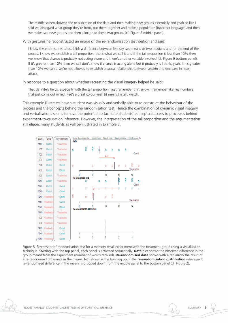
Figure 8. Screenshot of randomisation test for a memory recall experiment with the treatment group using a visualisation technique. Starting with the top panel, each panel is activated sequentially. Data plot shows the observed difference in the group means from the experiment (number of words recalled). Re-randomised data shows with a red arrow the result of a re-randomised difference in the means. not shown is the building up of the re-randomisation distribution where each re-randomised difference in the means is dropped down from the middle panel to the bottom panel (cf. Figure 2).


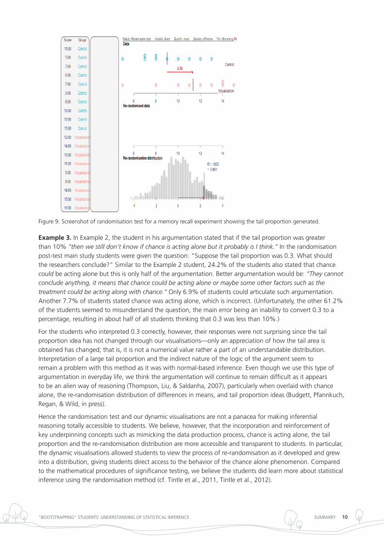
Figure 9. Screenshot of randomisation test for a memory recall experiment showing the tail proportion generated.

Example 3. in example 2, the student in his argumentation stated that if the tail proportion was greater than 10% “then we still don’t know if chance is acting alone but it probably is I think.” in the randomisation post-test main study students were given the question: “Suppose the tail proportion was 0.3. What should the researchers conclude?” Similar to the example 2 student, 24.2% of the students also stated that chance could be acting alone but this is only half of the argumentation. Better argumentation would be: “They cannot conclude anything, it means that chance could be acting alone or maybe some other factors such as the treatment could be acting along with chance.” only 6.9% of students could articulate such argumentation. Another 7.7% of students stated chance was acting alone, which is incorrect. (unfortunately, the other 61.2% of the students seemed to misunderstand the question, the main error being an inability to convert 0.3 to a percentage, resulting in about half of all students thinking that 0.3 was less than 10%.)

For the students who interpreted 0.3 correctly, however, their responses were not surprising since the tail proportion idea has not changed through our visualisations—only an appreciation of how the tail area is obtained has changed; that is, it is not a numerical value rather a part of an understandable distribution. interpretation of a large tail proportion and the indirect nature of the logic of the argument seem to remain a problem with this method as it was with normal-based inference. even though we use this type of argumentation in everyday life, we think the argumentation will continue to remain difficult as it appears to be an alien way of reasoning (thompson, liu, & Saldanha, 2007), particularly when overlaid with chance alone, the re-randomisation distribution of differences in means, and tail proportion ideas (Budgett, Pfannkuch, regan, & Wild, in press).

Hence the randomisation test and our dynamic visualisations are not a panacea for making inferential reasoning totally accessible to students. We believe, however, that the incorporation and reinforcement of key underpinning concepts such as mimicking the data production process, chance is acting alone, the tail proportion and the re-randomisation distribution are more accessible and transparent to students. in particular, the dynamic visualisations allowed students to view the process of re-randomisation as it developed and grew into a distribution, giving students direct access to the behavior of the chance alone phenomenon. Compared to the mathematical procedures of significance testing, we believe the students did learn more about statistical inference using the randomisation method (cf. tintle et al., 2011, tintle et al., 2012).


research Question 2: How can students be stimulated to develop inferential concepts and what type and level of inferential reasoning can they achieve?

to answer this question, two items from the tests will be discussed to illustrate the type and level of inferential reasoning students achieved.

Inference and the bootstrap method

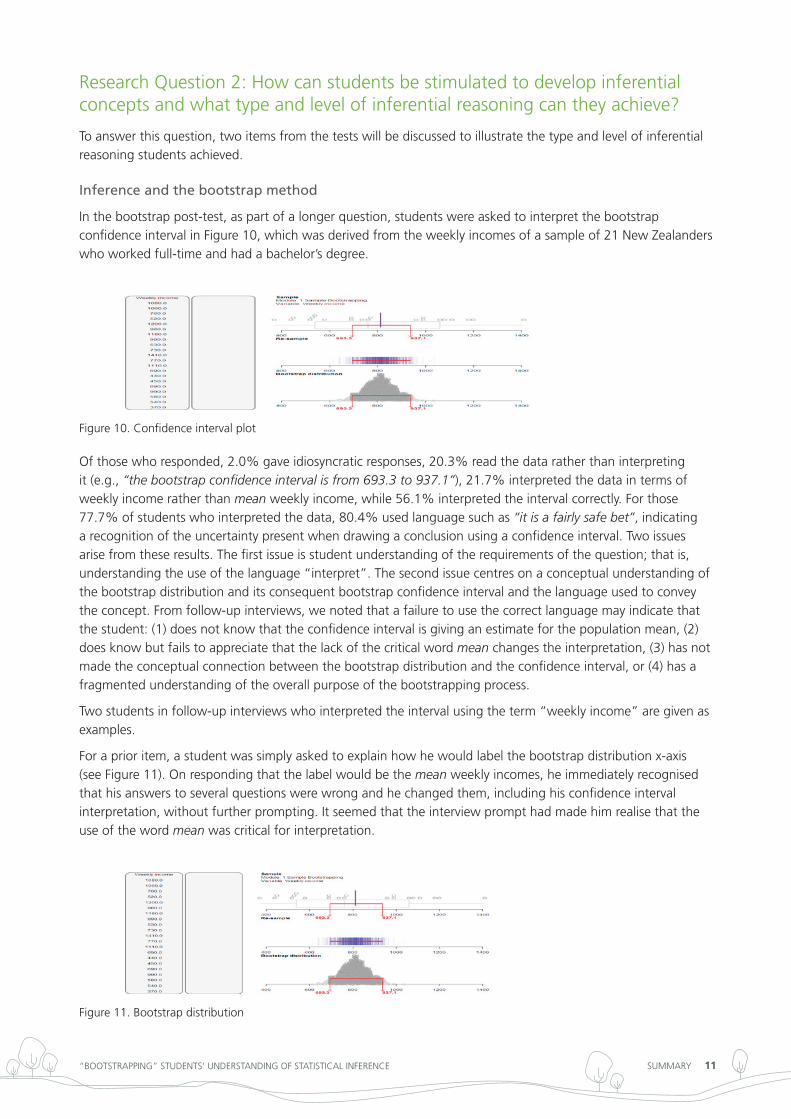
in the bootstrap post-test, as part of a longer question, students were asked to interpret the bootstrap confidence interval in Figure 10, which was derived from the weekly incomes of a sample of 21 new Zealanders who worked full-time and had a bachelor’s degree.

Figure 10. Confidence interval plot

of those who responded, 2.0% gave idiosyncratic responses, 20.3% read the data rather than interpreting it (e.g., “the bootstrap confidence interval is from 693.3 to 937.1”), 21.7% interpreted the data in terms of weekly income rather than mean weekly income, while 56.1% interpreted the interval correctly. For those 77.7% of students who interpreted the data, 80.4% used language such as “it is a fairly safe bet”, indicating a recognition of the uncertainty present when drawing a conclusion using a confidence interval. two issues arise from these results. the first issue is student understanding of the requirements of the question; that is, understanding the use of the language “interpret”. the second issue centres on a conceptual understanding of the bootstrap distribution and its consequent bootstrap confidence interval and the language used to convey the concept. From follow-up interviews, we noted that a failure to use the correct language may indicate that the student: (1) does not know that the confidence interval is giving an estimate for the population mean, (2) does know but fails to appreciate that the lack of the critical word mean changes the interpretation, (3) has not made the conceptual connection between the bootstrap distribution and the confidence interval, or (4) has a fragmented understanding of the overall purpose of the bootstrapping process.

two students in follow-up interviews who interpreted the interval using the term “weekly income” are given as examples.

For a prior item, a student was simply asked to explain how he would label the bootstrap distribution x-axis (see Figure 11). on responding that the label would be the mean weekly incomes, he immediately recognised that his answers to several questions were wrong and he changed them, including his confidence interval interpretation, without further prompting. it seemed that the interview prompt had made him realise that the use of the word mean was critical for interpretation.

Figure 11. Bootstrap distribution


Another student recalled from the hands-on activity that the bootstrap distribution was a plot of the re-sample means and when asked to clarify the difference between weekly income and mean weekly income she said:

For the weekly, just the weekly income they would be different pays, different incomes. they can’t say precisely

which one each person would get. So with the typical one [mean one] they would get the confidence interval and

they can just assume that they get paid between this and this, because not every person gets paid the exact same.

She knew that for the mean weekly income, one obtains a confidence interval, she knew that the interval was derived from re-sample means and the label on the bootstrap distribution would be the average, she verbalised the words “typical”, “mean”, “median”, and “average”, and yet she still believed her interpretation to be true. it seemed that this student had a fragmented understanding of the overall purpose of confidence intervals and a tenuous grasp on the correct use of statistical language.

in the student interviews, however, it seemed that prompting the use of visual imagery from the dynamic visualisations or the hands-on activities stimulated students to step closer towards a better understanding of how to reason from confidence intervals.

Inference and the randomisation test

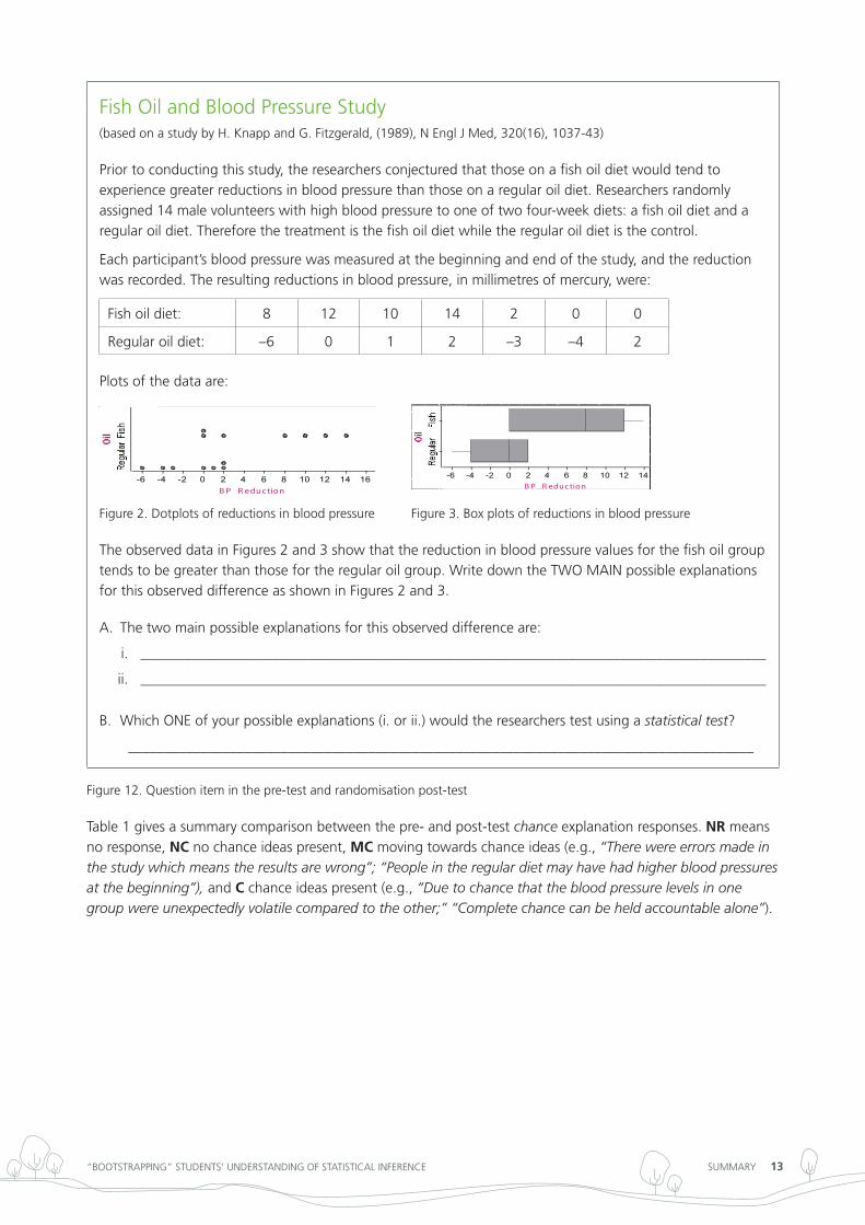
in the pre- and post-test students were asked to give two possible explanations for the observed difference for an experiment (see Figure 12). Many students were able to identify treatment explanations for the observed difference in the pre-test (79.2% of those who responded) but chance explanations were lacking. (note that half the students did the post-test question and 827 of these students sat both tests.)


Fish oil and Blood Pressure Study(based on a study by H. Knapp and g. Fitzgerald, (1989), n engl J Med, 320(16), 1037-43)

Prior to conducting this study, the researchers conjectured that those on a fish oil diet would tend to experience greater reductions in blood pressure than those on a regular oil diet. researchers randomly assigned 14 male volunteers with high blood pressure to one of two four-week diets: a fish oil diet and a regular oil diet. therefore the treatment is the fish oil diet while the regular oil diet is the control.

each participant’s blood pressure was measured at the beginning and end of the study, and the reduction was recorded. the resulting reductions in blood pressure, in millimetres of mercury, were:

Fish oil diet: 8 12 10 14 2 0 0

regular oil diet: –6 0 1 2 –3 –4 2

Plots of the data are:

-6 -4 -2 0 2 4 6 8 10 12 14 16B P _R educ tion

Collection 1 Box Plot

-6 -4 -2 0 2 4 6 8 10 12 14 16B P _R educ tion

Collection 1 Dot Plot

Figure 2. dotplots of reductions in blood pressure Figure 3. Box plots of reductions in blood pressure

the observed data in Figures 2 and 3 show that the reduction in blood pressure values for the fish oil group tends to be greater than those for the regular oil group. Write down the tWo MAin possible explanations for this observed difference as shown in Figures 2 and 3.

the two main possible explanations for this observed difference are:A.

______________________________________________________________________________________i.

______________________________________________________________________________________ii.

Which one of your possible explanations (i. or ii.) would the researchers test using a B. statistical test?

______________________________________________________________________________________

Figure 12. Question item in the pre-test and randomisation post-test

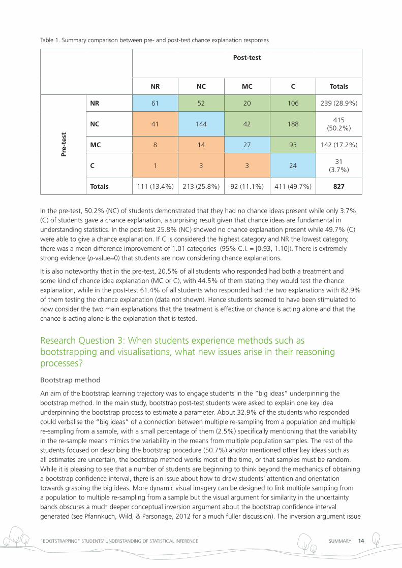
table 1 gives a summary comparison between the pre- and post-test chance explanation responses. NR means no response, NC no chance ideas present, MC moving towards chance ideas (e.g., “There were errors made in the study which means the results are wrong”; “People in the regular diet may have had higher blood pressures at the beginning”), and C chance ideas present (e.g., “Due to chance that the blood pressure levels in one group were unexpectedly volatile compared to the other;” “Complete chance can be held accountable alone”).


table 1. Summary comparison between pre- and post-test chance explanation responses

Post-test

NR NC MC C Totals

Pre-

test

NR 61 52 20 106 239 (28.9%)

NC 41 144 42 188415

(50.2%)

MC 8 14 27 93 142 (17.2%)

C 1 3 3 2431

(3.7%)

Totals 111 (13.4%) 213 (25.8%) 92 (11.1%) 411 (49.7%) 827

in the pre-test, 50.2% (nC) of students demonstrated that they had no chance ideas present while only 3.7% (C) of students gave a chance explanation, a surprising result given that chance ideas are fundamental in understanding statistics. in the post-test 25.8% (nC) showed no chance explanation present while 49.7% (C) were able to give a chance explanation. if C is considered the highest category and nr the lowest category, there was a mean difference improvement of 1.01 categories (95% C.i. = [0.93, 1.10]). there is extremely strong evidence (p-value≈0) that students are now considering chance explanations.

it is also noteworthy that in the pre-test, 20.5% of all students who responded had both a treatment and some kind of chance idea explanation (MC or C), with 44.5% of them stating they would test the chance explanation, while in the post-test 61.4% of all students who responded had the two explanations with 82.9% of them testing the chance explanation (data not shown). Hence students seemed to have been stimulated to now consider the two main explanations that the treatment is effective or chance is acting alone and that the chance is acting alone is the explanation that is tested.

research Question 3: When students experience methods such as bootstrapping and visualisations, what new issues arise in their reasoning processes?

Bootstrap method

An aim of the bootstrap learning trajectory was to engage students in the “big ideas” underpinning the bootstrap method. in the main study, bootstrap post-test students were asked to explain one key idea underpinning the bootstrap process to estimate a parameter. About 32.9% of the students who responded could verbalise the “big ideas” of a connection between multiple re-sampling from a population and multiple re-sampling from a sample, with a small percentage of them (2.5%) specifically mentioning that the variability in the re-sample means mimics the variability in the means from multiple population samples. the rest of the students focused on describing the bootstrap procedure (50.7%) and/or mentioned other key ideas such as all estimates are uncertain, the bootstrap method works most of the time, or that samples must be random. While it is pleasing to see that a number of students are beginning to think beyond the mechanics of obtaining a bootstrap confidence interval, there is an issue about how to draw students’ attention and orientation towards grasping the big ideas. More dynamic visual imagery can be designed to link multiple sampling from a population to multiple re-sampling from a sample but the visual argument for similarity in the uncertainty bands obscures a much deeper conceptual inversion argument about the bootstrap confidence interval generated (see Pfannkuch, Wild, & Parsonage, 2012 for a much fuller discussion). the inversion argument issue


is not currently part of students’ reasoning process and the question remains about whether, how and when it should be introduced to students.

Randomisation test

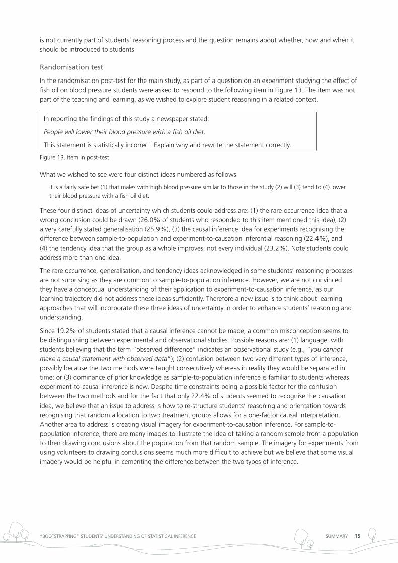
in the randomisation post-test for the main study, as part of a question on an experiment studying the effect of fish oil on blood pressure students were asked to respond to the following item in Figure 13. the item was not part of the teaching and learning, as we wished to explore student reasoning in a related context.

in reporting the findings of this study a newspaper stated:

People will lower their blood pressure with a fish oil diet.

this statement is statistically incorrect. explain why and rewrite the statement correctly.

Figure 13. item in post-test

What we wished to see were four distinct ideas numbered as follows:

it is a fairly safe bet (1) that males with high blood pressure similar to those in the study (2) will (3) tend to (4) lower

their blood pressure with a fish oil diet.

these four distinct ideas of uncertainty which students could address are: (1) the rare occurrence idea that a wrong conclusion could be drawn (26.0% of students who responded to this item mentioned this idea), (2) a very carefully stated generalisation (25.9%), (3) the causal inference idea for experiments recognising the difference between sample-to-population and experiment-to-causation inferential reasoning (22.4%), and (4) the tendency idea that the group as a whole improves, not every individual (23.2%). note students could address more than one idea.

the rare occurrence, generalisation, and tendency ideas acknowledged in some students’ reasoning processes are not surprising as they are common to sample-to-population inference. However, we are not convinced they have a conceptual understanding of their application to experiment-to-causation inference, as our learning trajectory did not address these ideas sufficiently. therefore a new issue is to think about learning approaches that will incorporate these three ideas of uncertainty in order to enhance students’ reasoning and understanding.

Since 19.2% of students stated that a causal inference cannot be made, a common misconception seems to be distinguishing between experimental and observational studies. Possible reasons are: (1) language, with students believing that the term “observed difference” indicates an observational study (e.g., “you cannot make a causal statement with observed data”); (2) confusion between two very different types of inference, possibly because the two methods were taught consecutively whereas in reality they would be separated in time; or (3) dominance of prior knowledge as sample-to-population inference is familiar to students whereas experiment-to-causal inference is new. despite time constraints being a possible factor for the confusion between the two methods and for the fact that only 22.4% of students seemed to recognise the causation idea, we believe that an issue to address is how to re-structure students’ reasoning and orientation towards recognising that random allocation to two treatment groups allows for a one-factor causal interpretation. Another area to address is creating visual imagery for experiment-to-causation inference. For sample-to-population inference, there are many images to illustrate the idea of taking a random sample from a population to then drawing conclusions about the population from that random sample. the imagery for experiments from using volunteers to drawing conclusions seems much more difficult to achieve but we believe that some visual imagery would be helpful in cementing the difference between the two types of inference.


limitations

the main limitation in this research study is ecological validity. Since bootstrapping and randomisation methods will be introduced into year 13 in 2013, many of the teachers implemented the learning trajectory outside normal school hours, teaching students before school, at lunch times or after school, which often resulted in fragmented delivery and attendance. Also, in a normal school programme, the two methods would not be taught consecutively. At the university level, introducing a new element into a very large course (2000 students) has many flow-on effects, including time constraints for assessing students for a research project. Hence a short learning trajectory was assessed when in fact students returned to these methods and ideas later on in the course. For the workplace students, a one-day course was set up, which is normal practice for such students. learning occurs over time and therefore any findings from this research are limited by time and delivery constraints imposed by working with students where qualifications are paramount.

Major implications

our research appears to show that the dynamic visualisations and learning trajectories that we created have the potential to make the concepts underpinning statistical inference more accessible and transparent to students. Shifting the learning of inferential statistics from a normal-distribution mathematics approach to a computer-based empirical approach is a major paradigm shift for teachers and the curriculum. Secondary teachers, examiners, moderators, teacher facilitators, resource writers, other stakeholders in the school system, and university and workplace lecturers will need professional development. Stakeholders will not only need to shift from a mathematical approach to a computer-based approach but also shift their pedagogy from a focus on sequential symbolic arguments towards more emphasis on a combined visual, verbal, and symbolic argumentation. these new computer-based methods require recognition at the government level that technology is an integral part of statistics teaching and learning and that professional development is essential.

developing students’ statistical inferential reasoning requires an understanding of the underpinning concepts and argumentation. these concepts and argumentation are intertwined with an understanding of the nature and precision of the language used. Students struggled to verbalise their understandings. We also struggled to define the underlying concepts and adequately and precisely communicate satisfactory verbalisations for the bootstrapping and randomisation method processes and the statistical inferential reasoning and argumentation used in the learning trajectories. Stimulating such thinking skills will require learning trajectories that involve hands-on activities, connected visual imagery, attention to adequate verbalisations, interpreting multiple representations, and learning to argue under uncertainty.

Within the statistical inference arena, students’ conceptualisation of inferential argumentation requires a re-structuring of their reasoning processes towards non-deterministic or chance argumentation coupled with an appreciation of causal argumentation for experimental studies. invoking mental images of the dynamic visualisations for the bootstrap and randomisation methods can help students to re-construct inference concepts. However, the tail proportion argumentation for the randomisation method, in common with any other form of significance testing, remains difficult for students to grasp. Similarly the inversion argument for the bootstrap confidence interval generated, in common with any other method, is difficult. An implication of these findings is that much more of statistical inference reasoning seems to be more accessible to students using these methods but some of the argumentation and ideas remain elusive and difficult to comprehend.

the new Zealand year 13 statistics curriculum and the related university introductory statistics course are leading the world, which has led to many international invitations. About 1200 teachers nationally have become aware of our innovative developments through our presentations and workshops. Also the project has led to increased leadership capacity and researcher capability in statistics education in new Zealand. therefore it is vital that more research is conducted into these new approaches to statistical inference and the consequent development of students’ reasoning processes and statistical argumentation.


references

Bakker, A. (2004). Design research in statistics education: On symbolizing and computer tools. utrecht, the netherlands: Cd-β Press, Center

for Science and Mathematics education.

Braun, V., & Clarke, V. (2006). using thematic analysis in psychology. Qualitative research in Psychology, 3(2), 77–101.

Budgett, S., Pfannkuch, M., regan, M., & Wild, C. J. (in press). dynamic visualisations and the randomization test. Technology Innovations

in Statistics Education.

Clark, J., & Paivio, A. (1991). dual coding theory and education. Educational Psychology Review, 3, 149–210.

Cobb, g. (2007). the introductory statistics course: A Ptolemaic curriculum? Technology Innovations in Statistics Education, 1(1), 1–15.

retrieved from http://escholarship.org/uc/item/6hb3k0nz

garfield, J., delMas, r., & Zieffler, A. (2012). developing statistical modelers and thinkers in an introductory, tertiary-level statistics course.

ZDM – The International Journal on Mathematics Education, 44(7), 883–898, doi: 10.1007/s11858-012-0447-5

gould, r., davis, g., Patel, r., & esfandiari, M. (2010). enhancing conceptual understanding with data driven labs. in C. reading (ed.), Data

and context in statistics education: Towards an evidence-based society. Proceedings of the Eighth International Conference on Teaching

Statistics, Ljubljana, Slovenia. Voorburg, the netherlands: international Statistical institute. retrieved from http://www.stat.auckland.

ac.nz/~iase/publications/icots8/iCotS8_C208_gould.pdf

Hesterberg, t. (2006). Bootstrapping students’ understanding of statistical concepts. in g. Burrill, & P. elliot, Thinking and reasoning with

data and chance: NCTM Yearbook (pp. 391–416). reston, VA: national Council of teachers of Mathematics.

Hjalmarson, M., & lesh, r. (2008). engineering and design research: intersections for education research and design. in A. Kelly, r. lesh, &

K. Baek (eds.), Handbook of design research methods in education: Innovations in science, technology, engineering, and mathematics

learning and teaching (pp. 96–110). new york, ny: routledge.

Holcomb, J., Chance, B., rossman, A., tietjen, e., & Cobb, g. (2010). introducing concepts of statistical inference via randomization tests.

in C. reading (ed.), Data and context in statistics education: Towards an evidence-based society. Proceedings of the Eighth International

Conference on Teaching Statistics, Ljubljana, Slovenia. Voorberg, the netherlands: international Statistical institute. retrieved from

http://www.stat.auckland.ac.nz/~iase/publications/icots8/iCotS8_8d1_HolCoMB.pdf

Parsonage, r., Pfannkuch, M., Wild, C.J., & Aloisio, K. (2012). Bootstrapping confidence intervals. Proceedings of the 12th International

Congress on Mathematics Education, Topic Study Group 12, 8–15 July, Seoul, Korea, (pp. 2613–2622). [uSB]. Seoul, Korea: iCMe-12.

retrieved from http://icme12.org/

Pfannkuch, M., Arnold, P., & Wild, C. (2011). Statistics: It’s reasoning, not calculating. Summary research report on building students’

inferential reasoning: Statistics curriculum levels 5 and 6. retrieved from http://www.tlri.org.nz/tlri-research/research-completed/school-

sector/building-students-inferential-reasoning-statistics

Pfannkuch, M., regan, M., Wild, C.J., Budgett, S., Forbes, S., Harraway, J., & Parsonage, r. (2011). inference and the introductory statistics

course. International Journal of Mathematical Education in Science and Technology, 42(7), 903-913.

Pfannkuch, M. & Wild, C.J. (2012). laying foundations for statistical inference. Proceedings of the12th International Congress on

Mathematics Education, Regular Lectures 1-9, 8-15 July, Seoul, Korea, (pp. 317–329). [uSB]. Seoul, Korea: iCMe-12. online: http://

icme12.org/

Pfannkuch, M., Wild, C. J., & Parsonage, r. (2012). A conceptual pathway to confidence intervals. ZDM – The International Journal on

Mathematics Education, 44(7), 899–911, doi: 10.1007/s11858-012-0446-6.

Pfannkuch, M., Wild, C. J., & regan, M. (in press). Students’ difficulties in practicing computer-supported statistical inference: Some

hypothetical generalizations from a study. in d. Frischemeier (ed.), Using tools for learning mathematics and statistics. Berlin: Springer

Spektrum.

Sotos, A., Vanhoof, S., noortgate, W., & onghena, P. (2007). Students’ misconceptions of statistical inference: A review of the empirical

evidence from research on statistics education. Educational Research Review, 2, 98–113.

thompson, P., liu, y., & Saldanha, l. (2007). intricacies of statistical inference and teachers’ understandings of them. in M. lovett & P. Shaw

(eds.), Thinking with data, (pp. 207–231). Mawah, nJ: erlbaum.

tintle, n., topliff, K., Vanderstoep, J., Holmes, V., & Swanson, t. (2012). retention of statistical concepts in a preliminary randomization-

based introductory statistics curriculum. Statistics Education Research Journal, 11 (1), 21–40. retrieved from http://www.stat.auckland.

ac.nz/~iase/serj/SerJ11%281%29_tintle.pdf

tintle, n., VanderStoep, J., Holmes, V., Quisenberry, B., & Swanson, t. (2011). development and assessment of a preliminary randomization-

based introductory statistics curriculum. Journal of Statistics Education, 19(1). retrieved from http://www.amstat.org/publications/jse/

v19n1/tintle.pdf

Wood, M. (2005). the role of simulation approaches in statistics. Journal of Statistics Education, 13(3), 1–11. retrieved from www.amstat.

org/publications/jse/v13n3/wood.html


Software

inZight data analysis free software, from www.stat.auckland.ac.nz/~wild/inZight/

nVivo qualitative data analysis software; QSr international Pty ltd. Version 9, 2010

r data analysis open-source software. http://cran.stat.auckland.ac.nz/

Website for resource materials, slides, and recorded talks http://new.censusatschool.org.nz/resources/?nzc_level=-1&keyword=-1&event=290&auth=-1&year_added=-1&search=1

Project team

Maxine Pfannkuch, Chris Wild, Stephanie Budgett, ross Parsonage, Matt regan, the university of Auckland.

Sharleen Forbes, School of government, Victoria university of Wellington

John Harraway, otago university

Sixteen year 13 teachers from various new Zealand schools (decile 3 to 10)

Six university lecturers

three teacher professional development facilitators

nick Horton, Smith College, Massachusetts, uSA .

Project contact

dr Maxine [email protected]+64 9 923 8794department of StatisticsAuckland universityPrivate Bag 92019Auckland 1142

Documents

“Bootstrapping” students’ understanding of statistical ... report.pdf · to develop students’ understanding of statistical inference concepts and ... some common pre-test