Bootstrapping for Significance of Compact Clusters inMulti-dimensional Datasets

Ranjan Maitra, Volodymyr Melnykov and Soumendra N. Lahiri ∗A bootstrap approach is proposed for assessing significance in the clustering of multi-dimensional datasets. Thedeveloped procedure compares two models and declares the more complicated model a better candidate if there issignificant evidence in its favor. The performance of the procedure is illustrated on two well-known classificationdatasets and comprehensively evaluated in terms of its ability to estimate the number of components via extensivesimulation studies, with excellent results. The methodology is also applied to the problem of k-means color quan-tization of several standard images in the literature, and demonstrated to be a viable approach for determining theminimal and optimal numbers of colors needed to display an image without significant loss in resolution.Keywords: bootstrap, overlap, hierarchical clustering, k-means algorithm, Prohorov metric, p-value quanti-tation map, q-value quantitation map

1. INTRODUCTION

Cluster analysis partitions datasets into groups such that observations within each class share common proper-ties, but are also considerably different from those in other groups. This is a difficult problem with many diverseapplications eg, taxonomical classification (Michener and Sokal, 1957), market segmentation (Hinneburg and Keim,1999) or software management (Maitra, 2001) with consequently, a large body of literature in statistics and machinelearning (see eg. Murtagh, 1985; Ramey, 1985; McLachlan and Basford, 1988; Kaufman and Rousseuw, 1990; Everittet al., 2001; Fraley and Raftery, 2002; Tibshirani and Walther, 2005; Kettenring, 2006; Xu and Wunsch, 2009).

One popular approach to clustering is model-based: here, a probability model specifies the distribution of anobservation in terms of a mixture of parametric distributions (Fraley and Raftery, 2002), with each mixture componentdescribing properties of a particular group in the dataset. We refer to Titterington et al. (1985) and McLachlan andPeel (2000) for details, but note that clustering in such contexts requires a final assignment step that allocates eachobservation to the group for which its posterior probability of classification is highest.

The other main approach to clustering is largely heuristic and model-free. Prominent among these are the distance-based methods, with a distance measure between every pair of observations (or groups of observations). These algo-rithms are further sub-divided into the hierarchical (Johnson, 1967; Everitt et al., 2001; Jain and Dubes, 1988) andthe partitional clustering algorithms which optimize some target function for a pre-specified number of clusters. Ex-amples of the latter range from the classical k-means (Forgy, 1965; MacQueen, 1967) and k-medoids (Kaufman andRousseuw, 1990) algorithms to the more modern approaches of competitive learning (Rumelhart and Zipser, 1985) orkernel-based clustering (Haykin, 1999; Xu and Wunsch, 2009).

An issue defying researchers in clustering is that of quantifying significance in the obtained groupings. Significanceassessment in the clustering context itself needs to be defined: we address this in terms of whether a more complicatedmodel (in terms of numbers of clusters, variables, estimable quantities, etc) is significantly better, in terms of its fit to adataset, than a simpler model or whether any improvement can be explained purely as a matter of chance. We developmethodology in this paper for the case of the model-free clustering methods using the bootstrap.

Closely related to our look at significance assessment is that of estimating the number of clusters (in this paper,K) in a dataset: this long-standing issue (Everitt, 1979) has many suggested approaches (Milligan and Cooper, 1985;McLachlan and Peel, 2000). Suggestions in the distance-based case include Marriott (1971)’s criterion and its variantsand the popular Gap statistic (Tibshirani et al., 2003). McLachlan (1987) suggests some approaches for model-basedclustering that successively test for K against K∗(> K) components, stopping when the null hypothesis can no

∗Ranjan Maitra is Professor in the Department of Statistics and Statistical Laboratory, Iowa State University, Ames, IA 50011-1210, VolodymyrMelnykov is Assistant Professor in the Department of Statistics, North Dakota State University, Fargo, ND 50373, and Soumendra N. Lahiri isProfessor in the Department of Statistics at Texas A& M University. This research was supported in part by the National Science FoundationCAREER Grant # DMS-0437555. The authors thank the Editor, an Associate Editor and three reviewers whose thoughtful comments greatlyimproved the content and presentation of this article.

1

longer be rejected, but development here has been muted by the need to account for possible regularity conditionviolations (Cramer, 1946). Challenges in implementation notwithstanding however, testing-based approaches provideat least one major advantage over the others, in that the results can be quantified in terms of the p-value, which is anuniversally understood measure between 0 and 1. Other approaches, while also quantitative, provide numerical valuesthat are data- and context-dependent. For instance, Marriott’s criterion which penalizes the logarithm of the deter-minant of the within-sums-of-squares-and-products matrix (W ) by twice the log of the number of clusters providesa numerical value: however, the magnitude changes from one dataset to the other. There is thus no context-free andreadily-interpretable quantification of the derived values, with no clear guidance on what differences in values are largeand what are not. It is this more-interpretable quantification of the p-value that encourages us to give testing-basedapproaches another look at quantifying significance.

There has been some recent work in assessing significance in the derived clusterings. McShane et al. (2002)and Liu et al. (2008) use parametric mixture model assumptions and the bootstrap to individually test whether eachof the derived groups can be further sub-divided into two, with allowances for high-dimensional low sample size(HDLSS) datasets, which forms the sole focus of their papers. (The use of the bootstrap in clustering is, however,of less recent vintage, having been employed (Kerr and Churchill, 2001; Dudoit and Fridlyand, 2003) to improve thereliability of clustering algorithms.) More recently, Maitra and Melnykov (2010a) derived an approximate approachfor significance assessment in mixture models and model-based clustering. They developed a quantitation map whichprovides a researcher with a detailed quantitative measure summarizing evidence against simpler models and in favorof more complicated alternatives. Their derivations are however inapplicable in the context of more heuristic andparametric-model-free clustering methods.

In this paper, we provide a bootstrap approach for quantifying such clustering methods. We assume that we havecompact groups which after some local transformation are spherical and similar to the other clusters. Under thisframework, we develop in Section 2 a distribution-free bootstrap strategy for testing a particular clustering setup vis-a-vis a more complicated one, i.e., we test between a null K- and an alternative K∗-clusters model. To fix ideas forthe development of our methodology here, we assume that K∗ > K and that data partitions with more clusters aresomehow always more complicated than those with fewer groups. We emphasize that this assumption is solely forexpediency and ease of presentation in this paper: our methodology also applies to other scenarios. The performanceof our approach is illustrated on two well-known classification datasets in Section 3 and evaluated in terms of itsability to estimate the number of significant groups through a series of simulation experiments in Section 4. Theconsistency of the bootstrap methodology for our problem is theoretically explored in Section 5. We next illustrateutility of our methodology in Section 6 to the novel application of determining the number of colors required toadequately represent a digital image. This paper concludes with some discussion in Section 7 along with an outlineof some possible directions for future work. We also have a supplement providing some additional illustrations andperformance evaluations. Sections, figures and tables in the supplement referred to in this paper are labeled with theprefix “S-”.

2. METHODOLOGY

2.1 Background and Preliminaries

LetX1,X2, . . . ,Xn be a random sample of n p-dimensional observations. We assume that eachXi ∼∑Kk=1 ζikfk(x),

where K is the number of groups, ζik = I(Xi∈Gk), and fk is the density of an observation in the kth cluster. Here I(·)is the indicator function and Gk is the set of observations in the sample belonging to the k-th cluster. The primary objec-tive is to estimateK and ζiks for i = 1, 2, . . . , n and k = 1, 2, . . . ,K in the presence of the nuisance parameters fk(·).We assume that for each k = 1, 2, . . . ,K, there exists a function Ψk : IRp → IRp such that g(x) = fk(Ψk(x))|JΨk

|where |JΨk

| is the Jacobian of Ψk and g(x) is a density centered at the origin with spherical level hyper-surfaces, i.e.for any orthogonal p × p-matrix Γ, g(x) = g(Γx). Further g(y) =

∏pj=1 h(yj) for y = (y1, y2, . . . , yp) where h(·)

is an univariate density symmetric about zero. This is the most general formulation, but in this paper, we consideronly those cases which result in center-based clusterings. For instance, when Ψk(x) ≡ x − µk, then each group hasthe same density but for location given by µk and we essentially assume that we have homogeneous spherical clus-ters. This is the putative framework underlying the k-means and other Euclidean distance-based clustering algorithms.When Ψk(x) ≡ Σ−

12 (x−µk), we assume having ellipsoidal clusters of different shapes and orientations centered at

the µks and Mahalanobis’ distance-based clustering methods would be most appropriate.

2

2.2 A Hypothesis-testing Framework

Suppose we want to investigate if there is significant evidence that the given dataset is better described by K∗

compact groups than by K clusters, where K∗ > K. The null and alternative hypotheses can then be prescribed inthe form H0 : F ∈ FK vs. Ha : F ∈ FK∗ ,where F represents the true distribution of the observations in the dataset,and FK and FK∗ represents the family of distributions under the null and alternative hypothesis respectively. The ithobservation has density of the form

∑Kk=1 ζ

(K)ik f

(K)k (x) under H0 and

∑K∗

k=1 ζ(K∗)ik f

(K∗)k (x) under Ha.

2.2.1 Test statistic

This paper uses as the test statistic the improvement in the within-cluster-sum-of-squares sK;K∗ = WK −WK∗ ,where WK =

∑ni=1

∑Kk=1 ζ

(K)ik (xi − µk)′(xi − µk), the optimized objective function for terminated k-means al-

gorithms that is obtained as its by-product when used to group a dataset into K clusters. Note, however, that whilewe develop methodology here using sK;K∗ as our test statistic, our development is general enough to also extend toother reasonable test statistics. Note also that sK;K∗ ≥ 0 always, since Wk decreases as K increases: our objective isto assess the significance in the improvement of WK upon fitting the dataset with a K∗-cluster model over that withonly K components. To do so, we have to calculate the p-value of the test statistic in terms of the probability that asK;K∗ from a true K-cluster model is greater than the sK;K∗ calculated from the dataset. We develop approaches toestimating this p-value next.

2.3 Obtaining a reference distribution

2.3.1 Homogeneous spherical clusters

We first develop methodology for homogeneous clusters. Under the null hypothesis ofK groups, we have a sampleΞ = {X1,X2, . . . ,Xn} from the joint distribution

n∏i=1

K∑k=1

ζ(K)ik

1

σg

(xi − µk

σ

), (1)

where g : IRp → IRp is invariant under orthogonal transformations. Our objective is to obtain the null distribution ofsK;K∗ under the assumption that the data are realizations from (1).

In obtaining the null distribution, we note that µks, ζ(K)ik s, σ and g(·) are all parameters of our null distribu-

tion. We use the K-clusters solution to the dataset to obtain estimates ζ(K)ik s, µk =

∑ni=1 ζ

(K)ik Xi/

∑ni=1 ζ

(K)ik and

σ = 1np

∑ni=1

∑Kk=1 ζ

(K)ik (Xi − µk)′(Xi − µk). Note that once the effects of the assigned centers µk and common

scale σ have been removed from each observation (using the K-clusters solution), then the residuals ε1, ε2, . . . , εn,where εi = (Xi −

∑Kk=1 ζ

(K)ik µk)/σ for i = 1, 2, . . . , n, form a sample from the common density g(·). A naıve

approach to estimating g(·) and using the bootstrap would resample from these εis. This naıve approach would,specifically, involve obtaining ε?1, ε

?2, . . . , ε

?n by sampling with replacement from ε1, ε2, . . . , εn, and then constructing

the resampled realizations X?i =

∑Kk=1 ζ

(K)ik µk + ε?i , i = 1, 2, . . . , n. Theorem 5.1 shows that such a resampling

strategy has low power, especially in the case when H0 specifies far fewer groups than the true. Additional illustra-tion of these claims is provided in the supplemental file: in particular, see Figure S-1. Thus, a carefully-designedresampling strategy is needed.

Note that g(·) is assumed to have spherical level hyper-surfaces and is defined through the univariate density h(·).Given this special structure for g(·), we note that the ordered set of normed residuals ‖ε(1)‖ ≤ ‖ε(2)‖ ≤ . . . ≤‖ε(n)‖ is sufficient for g(·). Thus, the conditional distribution of ε1, ε2, . . . , εn given the ordered set of normedresiduals ‖ε(1)‖, ‖ε(2)‖, . . . , ‖ε(n)‖ is free of g(·). We use this fact to obtain our resampled realizations. Note also thattransforming εi to Γiεi, i = 1, 2, . . . , n, where Γi is any p× p orthogonal matrix, maintains the ordered set of normedresiduals ‖ε(1)‖, ‖ε(2)‖, . . . , ‖ε(n)‖. Thus, a resampling strategy for the residuals would involve randomly samplingp-dimensional unit direction vectors, scaling them first with the magnitude of the residuals ‖ε(i)‖ and then with σ andshifting by the appropriate µk corresponding to ζ(K)

ik .Formally therefore, we propose the following: for each i = 1, 2, . . . , n, first generate a random unit direction

in p-dimensional space. We do so by simulating a p-variate standard normal random vector Zi, and let W i =Zi/‖Zi‖. Note that we use a standard p-variate Gaussian distribution random to obtain our normed realization, but

3

(a) K = 2,R = 0.5 (b) K = 3,R = 0.746 (c) K = 4,R = 1.0 (d) K = 5,R = 0.958

Figure 1. Ruspini dataset: k-means clustering solutions for different K. In each figure, colors represent true cluster-ings while characters represent the predicted groupings.

any distribution spherically symmetric around zero would also be appropriate, following Theorem 1 of Cambaniset al. (1981). We next obtain a random permutation (`1, `2, . . . , `n) of {1, 2, . . . , n}. Then, the ith resampled residualis given by ε∗i = ‖ε`i‖W i. Note that ‖ε∗i ‖ = ‖ε`i‖‖W i‖ = ‖ε`i‖‖Zi‖/‖Zi‖ = ‖ε`i‖, so that the resampledresiduals in the set {ε∗i ; i = 1, 2, . . . , n} maintain the norms in the set {εi; i = 1, 2, . . . , n}. (The directions of ε∗i sare however different from those in εis, following the effect of W i.) Adding these ε∗i s, after scaling with σ, to themeans of the corresponding cluster centers yields X∗i =

∑Kk=1 ζ

(K)ik µk + σε∗i for each i = 1, 2, . . . , n. Thus, we

get a resampled realization of the dataset under H0: Ξ∗ = {X∗1,X∗2, . . . ,X

∗n}. We replicate the procedure M times

to obtain resampled realizations of the dataset Ξ∗1,Ξ∗2, . . . ,Ξ

∗M . From each Ξ∗j , we obtain the test statistic given

by s∗j,(K;K∗), for j = 1, 2, . . . ,M . The p-value of sK;K∗ is then estimated by the proportion of cases in whichit is exceeded by the resampled s∗j,(K;K∗). Formally therefore, the p-value of the test statistic is calculated from1M

∑Mj=1 I

(s∗j,(K;K∗) > sK;K∗

), where I(·) is again the indicator function.

An Illustration We illustrate performance of our resampling mechanism on the synthetic Ruspini (1970) datasetwhich contains 75 bivariate observations from four well-separated groups that are each fairly spherical in their spread.This dataset, also available in the CLUSTER package in R, is popular for investigating clustering algorithms (Struyfet al., 1997). Figure 1 shows the optimal 2-, 3-, 4- and 5-cluster solutions obtained using the k-means algorithm,initialized here – as in all experiments reported in this paper – using the best (in terms of the smallest WK) of thedeterministic approach of Maitra (2009) and the partitioning obtained by using the hierarchical clustering algorithmwith Ward’s linkage. For each clustering, we also report the Adjusted Rand index (R) (Hubert and Arabie, 1985) whichmeasures similarity between two partitionings – in this case, the derived grouping and the true. (Note that R takes itsmaximum value of 1 when the two partitionings match perfectly. In general, values of R close to unity indicate goodclustering performance while those far below 1 are indicative of poorer performance.) In testing for the adequacy of a1-, 2-, 3-cluster solution vis-a-vis a solution with (say) 4 clusters, we need resampled datasets from the correspondingnull distribution. Figures S-2 (in the supplemental file) provide four resampled datasets each under null hypothesisassumptions of 1, 2, 3 and 4 clusters. The realizations for the first three sets appear quite different from the Ruspinidata so that any reasonable test statistic should have low probability of accepting H0 when challenged by a 4-groupmodel. On the other hand, when testing under a H0 of four true groups in the dataset, resampled datasets (refer againto Figures S-2) look quite similar to that of the observed data so that the test statistic will have a lower chance ofrejecting H0. We return to this dataset a little later in Section 3, moving instead to generalizing our methodology forcases beyond homogeneous spherical clusters.

2.3.2 Extension to the case of general ellipsoidal clusters

The entire process can be easily adapted for the case of general ellipsoidal clusters. Under H0, our sample Ξ ={X1,X2, . . . ,Xn} is from the joint distribution with K groups given by

n∏i=1

K∑k=1

ζ(K)ik

1

det (Σk)g(Σ− 1

2

k (xi − µk)), (2)

4

where g : IRp → IRp is as in (1). Once again, noting that µks, ζ(K)ik s, Σks and g are all parameters under H0,

we use the K-clusters solution to the dataset and obtain estimates ζ(K)ik s, µk =

∑ni=1 ζ

(K)ik Xi/

∑ni=1 ζ

(K)ik and

Σk =∑ni=1 ζ

(K)ik (Xi − µk)(Xi − µk)′/

∑ni=1 ζ

(K)ik . After the effects of the assigned center and individual scale

have been removed from each observation, and writing each residual εi =∑Kk=1 ζ

(K)ik Σ

− 12

k (Xi −∑Kk′=1 ζ

(K)ik′ µk′)

for i = 1, 2, . . . , n, we are left with the same scenario as in Section 2.3.1. That is, we have ε1, ε2, . . . , εn fromthe common density g with spherical level hyper-surfaces and defined through the univariate density h. We obtainresampled residuals ε∗1, ε

∗2, . . . , ε

∗n in the same manner as before. Combining, our resampled realization from the null

distribution is given by Ξ∗ = {X∗1,X∗2, . . . ,Xn∗}, where X∗i =

∑Kk=1 ζ

(K)ik (µk + Σ

12

k ε∗i ) for each i = 1, 2, . . . , n.

As before, the procedure is replicated M times to obtain resampled realizations Ξ∗1,Ξ∗2, . . . ,Ξ

∗M under H0, from

each of which we get s∗j,(K;K∗), for j = 1, 2, . . . ,M . The p-value of the observed test statistic is again estimated by1M

∑Mj=1 I

(s∗j,(K;K∗) > sK;K∗

).

We refer to the supplemental file for an illustrative example of the methodology developed here (see Section S-2 and, in particular, Figures S-3 and S-4). Note that while the development here has been for the case of generalellipsoidal clusters, it is also potentially valid for clusters that are more general-shaped, as long as an appropriatetransformation Ψ, e.g. the multivariate Box-Cox transform, can be found (see Section S-5 for an illustrative two-dimensional example). We also note that our methodology is applicable only to the case of multi-dimensional datasets(i.e., p ≥ 2). It is, by construction, unlikely to be able to generate a rich ensemble of realizations from the nulldistribution for one-dimensional observations, without additional assumptions.

2.3.3 Null distribution with no clusters

Sections 2.3.1 and 2.3.2 developed methodology for simulating realizations from the null distribution with Kclusters. This methodology is however inapplicable for the case where the null distribution specifies no clustering inthe data (a case which we refer to here as K = 0). This is a scenario where the null distribution is uniform overthe support of the data, so we propose adopting Tibshirani et al. (2003)’s proposal of sampling from the uniformdistribution on the p-dimensional hyper-rectangle (used by the authors to decide on the number of clusters for the Gapstatistic).

2.4 Summarizing Significance via Quantitation Maps

Maitra and Melnykov (2010a) also developed the p-value quantitation map to provide comprehensive visualizationof the p-values for different tests in the context of mixture models. The rows of these two-dimensional upper-triangularmaps index the model under H0 while the columns denote the model under Ha. The intersection of a particular row-column pair yields the p-value of the test statistic for testing the corresponding H0 against the corresponding Ha.To address the issue of multiple significance, the authors proposed controlling for the expected false discovery rates(FDR) using Benjamini and Hochberg (1995), giving rise to the q-value quantitation map. We note that, as cautionedby a reviewer, these derived q-values are somewhat ad hoc because the simultaneous hypothesis tests being testedhave to be approximately independent for the methodology of Benjamini and Hochberg (1995) to apply. Our detailedexperiments in Sections 3 and 4, however, show that these quantitation maps work quite well in practice.

2.4.1 Application to choosing K

The p- and q-value quantitation maps allow us to assess the significance of a host of clustering solutions. One im-portant application of these maps is to obtain an optimal estimate ofK, from among a pre-specified range [Kmin,Kmax].The quantitation map drawn represents p- and q-values with K corresponding to the simpler model in H0 and the one(K∗) corresponding to the more complicated model as Ha. In this application, we assume that K∗ > K, though thisis not a constraining requirement – see Section 2.4.2. Maitra and Melnykov (2010a) suggest choosing the optimal Kfrom within the range [Kmin,Kmax] by sequential testing using the following algorithm:

1. Let K = Kmin and K∗ = Kmin + 1.

2. If the q-value for testing H0 : K versus Ha : K∗ is less than the desired FDR (q0, say), reassign K ← K + 1and K∗ ← K∗ + 1. Otherwise, reassign K∗ ← K∗ + 1.

5

3. Reiterate Step 2 until K∗ > Kmax. Report the current (null) K as the number of clusters.

This scenario is less conservative than sequentially testing H0 : K versus Ha : K+ 1 clusters for K = Kmin,Kmin +2, . . . ,Kmax − 1 until the first instance for which q ≥ q0. We prefer the above approach because the failure to detectsignificance for some H0 : K versus Ha : K + 1 for some K does not necessarily rule out the possibility that anotherK∗-clustering solution for some K∗ > K + 1 would be significantly better than the K-solution.

2.4.2 Choosing between different clustering solutions

We conclude our discussion in this section by mentioning that the methodology in Section 2.4.1 can be readilygeneralized to make statements on the significance of many aspects of models. As a specific example, note that wecan use the above development to identify whether a more general K∗-clusters model is significantly better than a lesscomplicated model with K-groups, where complexity is determined based on a number of factors, eg. the numberof parameters being estimated under each hypothesis. We illustrate this generalization in Section 3.2.1 where weinvestigate groupings of the Iris dataset assuming spherical and general-shaped clusters.

3. ILLUSTRATIVE EXAMPLES

3.1 The Ruspini dataset

0

1

1

2

2

3

3

4

4

5

5

6

6

7

< 0.010.01 − 0.020.02 − 0.030.03 − 0.040.04 − 0.050.05 − 0.060.06 − 0.070.07 − 0.080.08 − 0.090.09 − 0.10> 0.10

Figure 2. The q-value quantitationmap for the Ruspini dataset.

Our first illustration is on the dataset of Section 2.3.1, clustered via k-means for different K. (For all cases in this paper, M = 1000.) The q-valuequantitation map (Figure 2) indicates that any clustering solution (K∗ > 0)is preferable over one with no clustering (K = 0), and that any of the K∗-group (K∗ > 1) partitions is significantly better (q < 0.05) than assuming ahomogeneous structure in the data (K = 1). Indeed, it appears that any of thepartitions obtained using K∗ > K groups for K∗ ≤ 7 is also significantlybetter than theK-groups partition, forK = 2, 3, but the same can not be saidfor when K = 4. Thus, we are led to prefer the model with K = 4 as it isthe first instance over which more complicated models are not significantlypreferred. Indeed, for this solution, we get a perfect match (R = 1.0), whileR = 0.5 and 0.746 for the 2- and 3-clusters solutions, respectively.

3.2 Iris dataset

Our next illustration is on the celebrated Iris dataset (Anderson, 1935;Fisher, 1936) having measurements on each of petal length and width andsepal length and width on 50 observations each drawn from three Iris species,namely I. setosa, I. versicolor and I. virginica. It is known that I. setosa is very clearly distinguished from the other twospecies while I. versicolor and I. virginica are more closely related and not as easily separated. We partition the datasetfor differentK using Gaussian model-based clustering with general dispersions – initialized using the emEM approachof Biernacki et al. (2003) – and then bootstrap for significance as per Section 2.3.2. Figures 3a–d present modifiedAndrews (1972) curves (formal description also provided in the supplemental file, vide Section S-3.1) for the 2-, 3-,4- and 5-groups partitionings, along with their R-values relative to the true group identifications. The distinctivenessof I. setosa from the other two species is very clear (supported by Figure S-3a of the supplement, which displaysthe true classification). The 3-group solution also shows some overlap between I. versicolor and I. virginica, whilethe 4- and 5- group solutions show these two species as being sub-divided further. Figure 3e displays the q-valuequantitation map: the no clustering assumption is clearly not tenable. We also notice significant improvements uponfitting larger K∗-groups-models (K∗ ≤ 6) over models with one or two groups. (In particular, q = 0.005 for testingH0 : K = 2 versusHa : K∗ = 3. The quantitation map also informs us that more complicated clustering solutions arenot significantly preferred over the 3-cluster model (q > 0.1 in all cases), thus three groups are adequate to describethe heterogeneity in the data. This solution also most closely matches the known classification (R = 0.904) for thedataset.

6

3.2.1 Choice of clustering algorithm

A reviewer wondered about the choice of mixtures-of-Gaussians-model-based clustering with general group-specific dispersions instead of, for instance, k-means clustering which inherently assumes a common spherical disper-sion structure for all groups. This interesting question can be answered by the development of Section 2.4.2. Figure 3fprovides the q-value quantitation map for comparing models fit using k-means (K ranging from 1 through 8) andmodel-based clustering (K varying from 1 through 4): here the models are ordered according to the number of param-eters reflecting model complexity. Thus, the model with fewer parameters (Kp for k-means,

(K+1

2

)p+Kp+K − 1

for model-based clustering) is in H0 (row) while that with the larger number of parameters is in Ha (column). Furthersupporting evidence in the form of Andrew’s curves andR-values of the k-means clustering solutions is in Figure S-5of the supplement. Figure 3f provides us with an understanding of several aspects: for instance, the solution with sevenhomogeneous spherical groups is significantly better (0.02 < q < 0.03) than the solution that places the I. setosa ob-servations in one cluster and the others in one other group. Also, if we restrict to only homogeneous spherical groups,no larger model fits the dataset significantly better (q > 0.10) than the 7-groups solution. (For clarity of presentation,Figure 3f does not display models with more than 8 homogeneous spherical groups.) But the 3-cluster model withgeneral group-specific dispersions is our optimal choice, and most appropriately so, since its R-value again indicatesthat it most closely fits the data.

(a) K = 2,R = 0.568 (b) K = 3,R = 0.904 (c) K = 4,R = 0.840

(d) K = 5,R = 0.732

0

1

1

2

2

3

3

4

4

5

5

6

< 0.010.01 − 0.020.02 − 0.030.03 − 0.040.04 − 0.050.05 − 0.060.06 − 0.070.07 − 0.080.08 − 0.090.09 − 0.10> 0.10

(e) q-value quantitation map for models withnon-spherical covariances

0

s1

s1

s2

s2

g1

g1

s3

s3

s4

s4

s5

s5

g2

g2

s6

s6

s7

s7

g3

g3

s8

s8

g4

< 0.010.01 − 0.020.02 − 0.030.03 − 0.040.04 − 0.050.05 − 0.060.06 − 0.070.07 − 0.080.08 − 0.090.09 − 0.10> 0.10

(f) q-value quantitation map for various models

Figure 3. (a-d) Andrews’ curves of Iris data colored according to the groupings obtained using Gaussian model-basedclustering with general group-specific dispersions for 2, 3, 4 and 5 groups, respectively. (e) The corresponding q-value quantitation map. (f) The q-value quantitation map for models fit using k-means and model-based clusteringwith different K. The letters “s” and “g” in the row and column labels are for k-means-obtained and model-based-clustering-obtained groupings respectively, while the numerals indicate the number of groups.

7

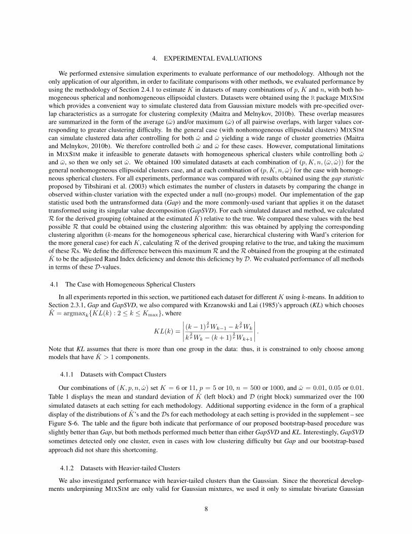
4. EXPERIMENTAL EVALUATIONS

We performed extensive simulation experiments to evaluate performance of our methodology. Although not theonly application of our algorithm, in order to facilitate comparisons with other methods, we evaluated performance byusing the methodology of Section 2.4.1 to estimate K in datasets of many combinations of p, K and n, with both ho-mogeneous spherical and nonhomogeneous ellipsoidal clusters. Datasets were obtained using the R package MIXSIMwhich provides a convenient way to simulate clustered data from Gaussian mixture models with pre-specified over-lap characteristics as a surrogate for clustering complexity (Maitra and Melnykov, 2010b). These overlap measuresare summarized in the form of the average (ω) and/or maximum (ω) of all pairwise overlaps, with larger values cor-responding to greater clustering difficulty. In the general case (with nonhomogeneous ellipsoidal clusters) MIXSIMcan simulate clustered data after controlling for both ω and ω yielding a wide range of cluster geometries (Maitraand Melnykov, 2010b). We therefore controlled both ω and ω for these cases. However, computational limitationsin MIXSIM make it infeasible to generate datasets with homogeneous spherical clusters while controlling both ωand ω, so then we only set ω. We obtained 100 simulated datasets at each combination of (p,K, n, (ω, ω)) for thegeneral nonhomogeneous ellipsoidal clusters case, and at each combination of (p,K, n, ω) for the case with homoge-neous spherical clusters. For all experiments, performance was compared with results obtained using the gap statisticproposed by Tibshirani et al. (2003) which estimates the number of clusters in datasets by comparing the change inobserved within-cluster variation with the expected under a null (no-groups) model. Our implementation of the gapstatistic used both the untransformed data (Gap) and the more commonly-used variant that applies it on the datasettransformed using its singular value decomposition (GapSVD). For each simulated dataset and method, we calculatedR for the derived grouping (obtained at the estimated K) relative to the true. We compared these values with the bestpossible R that could be obtained using the clustering algorithm: this was obtained by applying the correspondingclustering algorithm (k-means for the homogeneous spherical case, hierarchical clustering with Ward’s criterion forthe more general case) for each K, calculatingR of the derived grouping relative to the true, and taking the maximumof theseRs. We define the difference between this maximumR and theR obtained from the grouping at the estimatedK to be the adjusted Rand Index deficiency and denote this deficiency byD. We evaluated performance of all methodsin terms of these D-values.

4.1 The Case with Homogeneous Spherical Clusters

In all experiments reported in this section, we partitioned each dataset for differentK using k-means. In addition toSection 2.3.1, Gap and GapSVD, we also compared with Krzanowski and Lai (1985)’s approach (KL) which choosesK = argmaxk{KL(k) : 2 ≤ k ≤ Kmax}, where

KL(k) =

∣∣∣∣∣ (k − 1)2pWk−1 − k

2pWk

k2pWk − (k + 1)

2pWk+1

∣∣∣∣∣ .Note that KL assumes that there is more than one group in the data: thus, it is constrained to only choose amongmodels that have K > 1 components.

4.1.1 Datasets with Compact Clusters

Our combinations of (K, p, n, ω) set K = 6 or 11, p = 5 or 10, n = 500 or 1000, and ω = 0.01, 0.05 or 0.01.Table 1 displays the mean and standard deviation of K (left block) and D (right block) summarized over the 100simulated datasets at each setting for each methodology. Additional supporting evidence in the form of a graphicaldisplay of the distributions of K’s and theDs for each methodology at each setting is provided in the supplement – seeFigure S-6. The table and the figure both indicate that performance of our proposed bootstrap-based procedure wasslightly better than Gap, but both methods performed much better than either GapSVD and KL. Interestingly, GapSVDsometimes detected only one cluster, even in cases with low clustering difficulty but Gap and our bootstrap-basedapproach did not share this shortcoming.

4.1.2 Datasets with Heavier-tailed Clusters

We also investigated performance with heavier-tailed clusters than the Gaussian. Since the theoretical develop-ments underpinning MIXSIM are only valid for Gaussian mixtures, we used it only to simulate bivariate Gaussian

8

Table 1. Performance of the bootstrap-based methodology, gap statistic with and without svd, and KL method forestimating K homogeneous spherical clusters for different settings. The left half of the table provides the mean (K)and the corresponding standard deviation (σK) of the estimated number of clusters, while the right half shows themean (D) and standard deviation (σD) of the adjusted Rand index deficiencies.

ω

K(σK) D(σD)

K = 6, n = 500 K = 11, n = 1000 K = 6, n = 500 K = 11, n = 1000

p = 5 p = 10 p = 5 p = 10 p = 5 p = 10 p = 5 p = 10

Boo

tstr

ap 0.010 6.00 (0.00) 6.00 (0.00) 11.00 (0.00) 11.00 (0.00) 0.00 (0.00) 0.00 (0.00) 0.00 (0.00) 0.00 (0.00)0.050 5.94 (0.58) 6.00 (0.00) 10.80 (0.45) 11.00 (0.00) 0.00 (0.03) 0.00 (0.00) 0.01 (0.02) 0.00 (0.00)0.100 5.96 (0.28) 5.97 (0.22) 10.81 (0.49) 10.71 (0.57) 0.01 (0.03) 0.01 (0.03) 0.01 (0.02) 0.02 (0.03)

Gap

0.010 5.99 (0.10) 6.00 (0.00) 10.96 (0.40) 11.00 (0.00) 0.00 (0.00) 0.00 (0.00) 0.00 (0.02) 0.00 (0.00)0.050 5.91 (0.55) 6.00 (0.00) 10.77 (0.63) 11.00 (0.00) 0.00 (0.01) 0.00 (0.00) 0.01 (0.03) 0.00 (0.00)0.100 5.85 (0.52) 6.00 (0.00) 10.34 (1.67) 10.90 (1.00) 0.01 (0.04) 0.00 (0.00) 0.03 (0.12) 0.01 (0.09)

Gap

SVD 0.010 5.69 (1.20) 5.90 (0.70) 9.00 (4.02) 10.50 (2.19) 0.06 (0.23) 0.02 (0.14) 0.20 (0.40) 0.05 (0.22)

0.050 5.77 (0.93) 5.75 (1.10) 10.16 (2.56) 10.20 (2.73) 0.02 (0.14) 0.05 (0.20) 0.07 (0.24) 0.08 (0.26)0.100 5.14 (1.67) 5.46 (1.55) 9.11 (3.55) 9.50 (3.59) 0.12 (0.27) 0.09 (0.27) 0.15 (0.31) 0.13 (0.31)

KL

0.010 5.99 (0.30) 6.02 (0.20) 10.89 (0.65) 11.05 (0.30) 0.01 (0.02) 0.00 (0.01) 0.01 (0.04) 0.00 (0.01)0.050 5.94 (0.75) 6.17 (0.53) 10.51 (1.48) 11.13 (0.44) 0.02 (0.07) 0.01 (0.03) 0.03 (0.07) 0.00 (0.01)0.100 5.68 (1.02) 6.46 (0.81) 10.01 (2.38) 11.21 (0.70) 0.05 (0.09) 0.03 (0.04) 0.07 (0.17) 0.01 (0.02)

mixtures with homogeneous spherical dispersions for ω = 0.01, 0.05 and 0.10. To generate datasets however, wereplaced the Gaussian distribution in each coordinate with a tν distribution, where ν is the degrees of freedom. Tofacilitate illustration, we only considered K = 5, p = 2, n = 100. Our experimental suite consisted of the casesfor which ν = 3, 10 and ∞; the latter case is equivalent to realizations from a normal mixture. (Note that sinceMIXSIM is designed to simulate Gaussian mixtures, the actual overlap will be moderately to substantially higher, withdecreasing ν, than the pre-specified levels of Gaussian overlap as the tails of the tν distribution are heavier than thoseof the normal distribution.) Nevertheless, performance evaluations on these datasets provide us with an opportunity toinvestigate the performance of the bootstrap-based procedure in assessing significance in the presence of heavy-tailedclusters vis-a-vis ν. Figure 4 provides k-means-clustered datasets to illustrate the level of complexity associated withtν-distributed clusters, for ν = 3 and 10, and notional overlap ω = 0.005, 0.05, and 0.25. Figure 4 also providesthe q-value quantitation maps (first columns) and the partitioning (second columns) at the corresponding bootstrap-significance-estimated K for each dataset. Clearly, the cases with ν = 3 present substantially more complicateddatasets to partition than those for ν = 10. Note also that the quantitation maps in Figure 4 reflect clustering com-plexity very well. When ω is smaller, we are more confident about the choice of K. The increase in ν also makes thischoice easier. Thus, the two figures are also good illustrations of the use of quantitation maps in assessing significancein clustering.

The results of a more comprehensive simulation study over 100 datasets at each setting are summarized in Table 2and in the supplement (Figure S-7). Clearly, the overall results agree with our expectations and with the initial im-pressions from Figure 4: the performance of our procedure is substantially better than that of all three competitors –Gap, GapSVD or KL. The improvement in performance of our approach becomes more pronounced with increasedclustering complexity.

4.1.3 Performance with HDLSS datasets

Our next set of experiments in this setup of homogeneous spherical groups is a small-scale study for the case ofclustering in high-dimensional datasets, specifically for when we have low sample sizes. For this set of experiments, weobtained 100 80-dimensional datasets that were simulated from 4-component Gaussian mixtures with ω = 0.001 and0.01. Each dataset contained only 20 observations. The average number of detected clusters is 3.79 with σK = 0.40for ω = 0.001 and 3.52 with ω = 0.52 for ω = 0.01 correspondingly. Further, D was 0.08 with σD = 0.11 forω = 0.01 while D was 0.03 with σD = 0.05 for ω = 0.001. Thus, we have some indication that our procedure alsoworks well in clustering datasets that fall within the large p, small n framework.

4.2 Nonhomogeneous compact clusters

We used MIXSIM to generate 100 simulated datasets at each setting of (p,K, n, (ω, ω)), where p, K and n wereas before, while (ω, ω) = (0.001, 0.005), (0.001, 0.01), (0.01, 0.05), (0.01, 0.1) and (0.05, 0.25). For every simulated

9

0

1

1

2

2

3

3

4

4

5

5

6

6

7

7

8

< 0.010.01 − 0.020.02 − 0.030.03 − 0.040.04 − 0.050.05 − 0.060.06 − 0.070.07 − 0.080.08 − 0.090.09 − 0.10> 0.10

ω = 0.010 K = 4,R = 0.631

0

1

1

2

2

3

3

4

4

5

5

6

6

7

7

8

< 0.010.01 − 0.020.02 − 0.030.03 − 0.040.04 − 0.050.05 − 0.060.06 − 0.070.07 − 0.080.08 − 0.090.09 − 0.10> 0.10

ω = 0.010 K = 5,R = 0.787

0

1

1

2

2

3

3

4

4

5

5

6

6

7

7

8

< 0.010.01 − 0.020.02 − 0.030.03 − 0.040.04 − 0.050.05 − 0.060.06 − 0.070.07 − 0.080.08 − 0.090.09 − 0.10> 0.10

ω = 0.050 K = 3,R = 0.486

0

1

1

2

2

3

3

4

4

5

5

6

6

7

7

8

< 0.010.01 − 0.020.02 − 0.030.03 − 0.040.04 − 0.050.05 − 0.060.06 − 0.070.07 − 0.080.08 − 0.090.09 − 0.10> 0.10

ω = 0.050 K = 4,R = 0.784

0

1

1

2

2

3

3

4

4

5

5

6

6

7

7

8

< 0.010.01 − 0.020.02 − 0.030.03 − 0.040.04 − 0.050.05 − 0.060.06 − 0.070.07 − 0.080.08 − 0.090.09 − 0.10> 0.10

ω = 0.1 K = 3,R = 0.433

0

1

1

2

2

3

3

4

4

5

5

6

6

7

7

8

< 0.010.01 − 0.020.02 − 0.030.03 − 0.040.04 − 0.050.05 − 0.060.06 − 0.070.07 − 0.080.08 − 0.090.09 − 0.10> 0.10

ω = 0.1 K = 4,R = 0.587

Figure 4. Quantitation maps and estimated classifications (for the optimal K) for t-distributed datasets with 3 (leftpanel) and 10 (right panel) degrees of freedom with true K = 5, p = 2 and n = 100. In the figures representing theclassification of the datasets, symbols represent true classification while colors illustrate estimated classification.

dataset, we used hierarchical clustering with Ward’s criterion to partition the dataset into K groups for each K, fol-lowed by our bootstrap-based approach, Gap, and GapSVD to determine the suggested K by that method. For each ofthese datasets, we also used model-based clustering together with the Bayesian Information Criterion (BIC) to chooseK. We denote this method by BIC. Table 3 provides numerical summaries of the performance of our bootstrap-basedmethodology, Gap and GapSVD and BIC, with further supporting evidence provided in the supplement (specifically,Figure S-7). For datasets with low (ω, ω), or high separation between clusters, we observe low values of D and goodestimates for K. Expectedly, increased levels of overlap correspond to degraded performance all-around. Indeed, theproposed procedure underestimates K when overlap is substantial. That this is owing to clustering complexity andalgorithm becomes clear when we note that D-values remain remarkably low: this means that not all the clusters arealways clearly distinguishable. The comparison of our bootstrap-based approach with Gap, GapSVD and BIC suggeststhat the bootstrap procedure performed better in many cases, and even when clusters are poorly-separated. This pointsto a clear preference for our bootstrap-based method over the gap statistic and BIC in complicated clustering cases.Gap and GapSVD. We remark again that as per Figure S-8, the latter often chooses K = 1, especially when the overlap

10

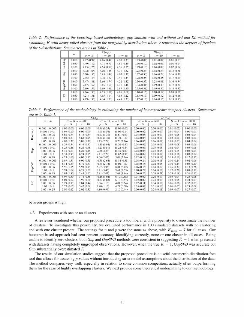
Table 2. Performance of the bootstrap-based methodology, gap statistic with and without svd and KL method forestimating K with heavy-tailed clusters from the marginal tν distribution where ν represents the degrees of freedomof the t-distributions. Summaries are as in Table 1.

ωK(σK) D(σD)

ν = 3 ν = 10 ν =∞ ν = 3 ν = 10 ν =∞

Boo

tstr

ap 0.010 4.77 (0.97) 4.86 (0.47) 4.90 (0.33) 0.03 (0.07) 0.01 (0.04) 0.01 (0.03)0.050 4.49 (1.17) 4.71 (0.70) 4.81 (0.49) 0.06 (0.10) 0.02 (0.06) 0.01 (0.04)0.100 4.15 (1.25) 4.54 (0.89) 4.76 (0.55) 0.09 (0.10) 0.04 (0.08) 0.02 (0.04)

Gap

0.010 3.72 (1.68) 4.08 (1.48) 4.31 (1.32) 0.23 (0.33) 0.18 (0.33) 0.13 (0.31)0.050 3.20 (1.56) 3.95 (1.44) 4.07 (1.37) 0.27 (0.30) 0.16 (0.28) 0.16 (0.30)0.100 2.95 (1.44) 3.78 (1.37) 3.91 (1.44) 0.28 (0.28) 0.16 (0.25) 0.17 (0.29)

Gap

SVD 0.010 3.47 (1.81) 3.66 (1.74) 4.22 (1.42) 0.30 (0.37) 0.28 (0.41) 0.16 (0.34)

0.050 2.87 (1.57) 3.85 (1.59) 4.11 (1.48) 0.34 (0.34) 0.19 (0.33) 0.17 (0.34)0.100 2.69 (1.56) 3.69 (1.49) 3.87 (1.50) 0.35 (0.31) 0.19 (0.30) 0.18 (0.32)

KL

0.010 4.76 (1.30) 4.75 (1.08) 4.86 (0.68) 0.10 (0.15) 0.08 (0.14) 0.03 (0.07)0.050 4.21 (1.31) 4.55 (1.14) 4.53 (1.22) 0.13 (0.17) 0.09 (0.12) 0.12 (0.16)0.050 4.19 (1.35) 4.14 (1.33) 4.48 (1.33) 0.12 (0.13) 0.14 (0.16) 0.13 (0.15)

Table 3. Performance of the methodology in estimating the number of heterogeneous compact clusters. Summariesare as in Table 1.

ω : ωK(σK) D(σD)

K = 6, n = 500 K = 11, n = 1000 K = 6, n = 500 K = 11, n = 1000p = 5 p = 10 p = 5 p = 10 p = 5 p = 10 p = 5 p = 10

Boo

tstr

ap

0.001 : 0.005 6.00 (0.00) 6.00 (0.00) 10.96 (0.35) 11.00 (0.00) 0.00 (0.00) 0.00 (0.00) 0.01 (0.03) 0.00 (0.00)0.001 : 0.01 5.99 (0.10) 6.00 (0.00) 11.01 (0.56) 11.00 (0.14) 0.00 (0.02) 0.00 (0.00) 0.01 (0.04) 0.00 (0.01)0.01 : 0.05 5.66 (0.74) 5.75 (0.54) 10.63 (1.36) 10.61 (0.99) 0.04 (0.05) 0.02 (0.03) 0.05 (0.05) 0.02 (0.04)0.01 : 0.1 5.69 (0.83) 5.68 (0.95) 10.24 (1.30) 10.70 (1.10) 0.04 (0.05) 0.04 (0.04) 0.03 (0.04) 0.03 (0.04)0.05 : 0.25 4.80 (1.31) 5.01 (1.71) 8.15 (2.29) 8.20 (2.16) 0.06 (0.06) 0.06 (0.07) 0.05 (0.03) 0.04 (0.04)

Gap

0.001 : 0.005 6.29 (0.54) 6.16 (0.37) 11.10 (0.98) 11.20 (0.40) 0.04 (0.07) 0.03 (0.06) 0.03 (0.08) 0.03 (0.06)0.001 : 0.01 6.25 (0.46) 6.26 (0.48) 11.23 (0.51) 11.22 (0.44) 0.03 (0.06) 0.03 (0.05) 0.02 (0.04) 0.03 (0.05)0.01 : 0.05 6.15 (0.61) 6.20 (0.45) 9.00 (2.33) 10.46 (0.99) 0.03 (0.06) 0.03 (0.05) 0.08 (0.15) 0.03 (0.04)0.01 : 0.1 6.38 (0.93) 6.74 (0.85) 9.11 (2.28) 10.62 (0.98) 0.04 (0.09) 0.03 (0.04) 0.08 (0.16) 0.03 (0.04)0.05 : 0.25 4.25 (1.60) 4.00 (1.92) 4.06 (2.03) 5.08 (2.14) 0.12 (0.18) 0.13 (0.18) 0.18 (0.16) 0.12 (0.12)

Gap

SVD

0.001 : 0.005 5.89 (1.31) 6.00 (0.55) 10.59 (2.64) 11.14 (0.35) 0.08 (0.24) 0.02 (0.11) 0.10 (0.24) 0.02 (0.06)0.001 : 0.01 6.14 (0.89) 6.10 (0.33) 10.61 (2.72) 11.00 (1.07) 0.05 (0.15) 0.02 (0.05) 0.10 (0.24) 0.03 (0.10)0.01 : 0.05 5.91 (1.15) 5.98 (0.79) 6.97 (3.96) 8.81 (3.42) 0.06 (0.16) 0.04 (0.12) 0.26 (0.32) 0.13 (0.26)0.01 : 0.1 5.99 (1.64) 6.25 (1.09) 8.11 (3.43) 9.61 (2.55) 0.10 (0.22) 0.04 (0.12) 0.17 (0.26) 0.08 (0.19)0.05 : 0.25 3.03 (1.80) 2.45 (1.62) 2.91 (2.07) 2.64 (1.94) 0.26 (0.25) 0.28 (0.21) 0.29 (0.18) 0.26 (0.15)

BIC

0.001 : 0.005 5.99 (0.30) 3.74 (0.56) 10.18 (1.02) 6.19 (0.68) 0.01 (0.07) 0.26 (0.10) 0.03 (0.04) 0.23 (0.06)0.001 : 0.01 6.09 (0.62) 3.96 (0.60) 10.37 (0.88) 6.10 (0.67) 0.02 (0.09) 0.24 (0.09) 0.03 (0.08) 0.24 (0.07)0.01 : 0.05 5.29 (0.83) 2.84 (0.44) 8.06 (1.13) 4.01 (0.64) 0.07 (0.11) 0.34 (0.10) 0.06 (0.06) 0.32 (0.09)0.01 : 0.1 5.27 (0.65) 3.47 (0.69) 7.90 (1.13) 4.27 (0.68) 0.05 (0.07) 0.21 (0.10) 0.06 (0.05) 0.29 (0.09)0.05 : 0.25 3.80 (0.62) 2.02 (0.35) 4.80 (0.99) 2.10 (0.44) 0.06 (0.07) 0.24 (0.11) 0.09 (0.07) 0.27 (0.07)

between groups is high.

4.3 Experiments with one or no clusters

A reviewer wondered whether our proposed procedure is too liberal with a propensity to overestimate the numberof clusters. To investigate this possibility, we evaluated performance in 100 simulated datasets with no clusteringand with one cluster present. The settings for n and p were the same as above, with Kmax = 7 for all cases. Ourbootstrap-based approach had cent percent accuracy, identifying correctly, none or one cluster in all cases. Beingunable to identify zero clusters, both Gap and GapSVD methods were consistent in suggesting K = 1 when presentedwith datasets having completely ungrouped observations. However, when the true K = 1, GapSVD was accurate butGap substantially overestimated K.

The results of our simulation studies suggest that the proposed procedure is a useful parametric-distribution-freetool that allows for assessing p-values without introducing strict model assumptions about the distribution of the data.The method compares very well, especially in relation to some common competitors, actually often outperformingthem for the case of highly overlapping clusters. We next provide some theoretical underpinning to our methodology.

11

5. CONSISTENCY RESULTS

5.1 On the inconsistency of the naıve bootstrap

Here we show that the naıve residuals-based bootstrap typically fails to reproduce the null distribution of the teststatistic. For concreteness, we work with p = 2 as in Figure S-1, and assume that there are K0-many true sphericalclusters, G1, . . . ,GK0 . For simplicity, we suppose that the points in the jth cluster are uniformly distributed over thedisc B(µj ; r), centered at unknown µj ∈ R2 and that the clusters are well-separated and also that they all have thesame scaling parameter.

Let G(K)j , i = 1, 2, . . . ,K denote the estimated partitions from a K-groups solution of the clustering algorithm.

Denote the jth cluster center by µj and as before, let εi = Xi −∑Kk=1 ζ

(K)ik µk, i = 1, 2, . . . , n be the residuals. In

order to approximate the null distribution of the test statistic sK,K∗ , the null distribution of the resampled bootstrapvariables must generate K spherical clusters. This, in particular, requires that the normalized residuals εi/‖εi‖,i = 1, . . . , n represent a random sample from the uniform distribution on the unit circle. Let G(K)(·) denote theempirical distribution of the normalized residuals εi/‖εi‖, i = 1, 2, . . . , n and let G denote the uniform distributionon the unit circle. The following theorem shows that for any K < K∗, and under some mild regularity conditions, thenaıve bootstrap method fails to approximate G consistently.

Theorem 5.1. Let Gj = {Xij : i = 1, 2, . . . , nj} denote the data in the jth cluster, so thatXij = µj +εij and {εij :i = 1, 2, . . . , nj , j = 1, . . . ,K0} are independently and uniformly distributed onB(0; r). Let n = n1+n2+. . .+nK0

and let |B| denote the size of a finite setB. Suppose, further, that the following conditions hold for some 1 ≤ K < K0:

(C.1) There exists ∆ > 0 such that B(µj , r + ∆) ∩H−j = ∅ where H−j is the convex hull of {µk : k 6= j, 1 ≤ k ≤K0}.

(C.2) Suppose that for all j = 1, 2, . . . ,K0, nj/n → π0j ∈ (0, 1) and that ∆ >

(π

2(π0min)2

− 1)r where π0

min =

min{π0j : 1 ≤ j ≤ K0}.

(C.3) Suppose that G(K)j ⊂ cone(θj(K), φj(K)) for some 0 ≤ θ

(K)1 < φ

(K)1 < θ

(K)2 < φ

(K)2 < . . . < θ

(K)K <

φ(K)K ≤ 2π} where cone(θ, φ) is the set of all points in R2 that lie in the cone emanating from the origin with

an angle ∈ [θ, φ] (with the x-axis).

Then, ∃ a constant δ0 > 0, depending only on {(µj , π0j ) : j = 1, . . . ,K0}, r, and K such that

P(

lim infn→∞

ρ(G(K), G) > δ0

)= 1,

where ρ(·) denotes the Prohorov metric (Billingsley, 1999) on the set of all probability measures on the unit circle andwhere π0

j ’s are as in Condition (C.2).

Proof. See Appendix A.

We discuss the implications of Theorem 5.1 and its conditions. Note that (C.1) above requires that the clustersbe well-separated while (C.2) says that in the limit there are K0 nontrivial clusters and that the parameter ∆ is largecompared to the radius r of each population cluster. Condition (C.3) stipulates that the clustering algorithm groupspoints from the adjacent clusters Gj’s and that the resulting clusters each contain one or more complete clusters Gjs.(We note that it is possible to prove a version of the theorem for clusters formed with split Gj-s, but only underadditional conditions on the structure of the clustering algorithm.) However, when the original clusters Gjs are well-separated, Condition (C.3) holds for many clustering algorithms. In particular, it always holds for any clusteringalgorithm when K = 1 and for any given K < K0 for the k-means algorithm, under suitable configurations ofµ1, . . . ,µK0

.It also follows from Theorem 5.1 that the empirical distribution of the normalized residuals from the naıve bootstrap

fails to approximate the uniform distribution on the unit circle even in the (weak) form of convergence in distribution,as the sample size becomes infinitely large. As a result, the naıve bootstrap method fails to give a valid approximationto the null distribution of the test statistic sK,K∗ when the conditions of the Theorem are satisfied, and therefore, anystep-up procedure based on the naıve bootstrap method for quantitation is inconsistent. In comparison, the uniformity

12

of the normalized residuals is directly built into the formulation of the modified bootstrap method proposed in thispaper and satisfies the key consistency condition:

ρ(G(K), G)→ 0 as n→∞, a.s. (3)

for all K < K0 where G(K) is the conditional distribution of the resampled error variable ε∗1 under the modifiedbootstrap method. Indeed, as the modified bootstrap error variables have the same distribution as Z/‖Z‖, where Zhas the standard multivariate normal distribution on Rd, it follows that ρ(G(K), G) = 0 for every K and every n, sothat (3) holds trivially.

5.2 Consistency of our suggested bootstrap procedure

Next we consider consistency of our suggested bootstrap procedure in somewhat more generality than in Section5.1. Specifically, we suppose that under the null hypothesis, there are K0 independent groups Gj = {Xij : i =

1, . . . , nj}, 1 ≤ j ≤ K0 and Xij has density g(x − µj) for all i, j, where g(·) is as in (1). Let Gj , j = 1, 2, . . . ,K0

denote the estimated groups from the K0-cluster solution, with respective cluster centers µj’s. To approximate thenull distribution of the test statistic SK0,K by our modified bootstrap, we follow the steps described in Section 2.3.Specifically, we generate the bootstrap error variables {ε∗1, ε∗2, . . . , ε∗n} as ε∗i = ‖ε`i‖Wi, i = 1, 2, . . . , n, wherethe residuals {εi : i = 1, 2, . . . , n} are obtained from the K0-cluster solution of the clustering algorithm and where{`1, `2, . . . , `n} is a (nonrandom) permutation of {1, 2, . . . , n}. We next show that under some regularity conditions,the (conditional) distribution of the bootstrap error variable ε∗1 under the modified bootstrap scheme provides a validapproximation to the null distribution of the error variable ε1. To that end, for j, k = 1, 2, . . . ,K0, let πj,k =

n−1∑nj

i=1 I(Xi ∈ Gk) denote the proportion of Xi’s from group Gj falling in the estimated cluster Gk. Also, let P∗denote the bootstrap probability and G denote the collection of all convex measurable subsets of Rp. Then we havethe following

Theorem 5.2. Suppose that under H0, Gj = {Xij : i = 1, 2, . . . , nj}, 1 ≤ j ≤ K0 are independent and Xij hasdensity g(x − µj) for all i, j, where g(·) is as in (1) and where nj/n → π0

j ∈ (0, 1) for all j. Further, assume thefollowing conditions:

(C.4) (i) For all j = 1, 2, . . . ,K0, µj → µj almost surely.

(ii) For all j, k = 1, 2, . . . ,K0, ∃ πj,k ∈ [0, 1] with πj,j = π0j 3 πj,k → πj,k almost surely.

Then,supC∈G

∣∣∣P∗(ε∗1 ∈ C)− P (ε1 ∈ C)∣∣∣→ 0 as n→∞, almost surely.

Proof. See Appendix B.

Condition (C.4) is a condition on the clustering algorithm: Specifically, Part (i) of (C.4) says that under H0, thecluster centers converge to the true cluster centers almost surely. (In particular, this condition holds for the k-meansalgorithm (cf. Pollard, 1981)). Additionally, Part (ii) of Condition (C.4) says that the clustering algorithm reproducesthe proportion of points in the true clusters, asymptotically. Since

∑K0

k=1 πj,k = nj/n→ π0j = πj,j∀j, it follows that∑

k 6=j πj,k = 0. As a result, under (C.4)(ii), the number of points in the jth cluster that are wrongly clustered is o(n)for every j = 1, 2, . . . ,K0. This is a weak requirement on the clustering algorithm which allows a large number ofpoints to be clustered incorrectly, for large n.

Theorem 5.2 shows that under the conditions stated above, the modified bootstrap algorithm can successfullycapture the distribution of the error variables, almost surely. Since the test statistic sK0,K is a smooth function of theerror variables {ε1, ε2, . . . , εn} (given, in the case of this paper, by a difference of sums of squares), it follows thatthe modified bootstrap method can be used to approximate the null distribution of sK0,K . In contrast, as shown byTheorem 5.1. the naıve bootstrap method typically fails to reproduce the null distribution of the errors and hence, failsto provide a valid reference distribution for the test statistic sK0,K .

6. APPLICATION TO COLOR QUANTIZATION

Color quantization is used in computer graphics to reduce the number of colors in an image without appreciablylosing its visual quality. The importance of this process comes from a need to display images on devices that are not

13

completely capable of dealing with multicolor images. It is also used for some image storing standards such as theGraphics Interchange Format (GIF).

Each pixel in an image is represented in terms of a mixture of red, green and blue colors with different intensities.This way of storing a color is known as RGB format. Hence, every picture can be presented as a three-dimensionaldataset with the number of observations depending on the size of the picture. For example, an image of size 256×256can be transformed into a dataset with 65,536 observations and a 512 × 512 image can be represented as a dataset ofsize 262,144. k-means color quantization applies the k-means algorithm, suitably initialized, to such a dataset to yielda palette of k colors for representing the image. Further, while k-means represents one of several approaches to colorquantization (Emre Celebi, 2011), note also that K needs to be specified in k-means color quantization.

We apply our bootstrapping-for-significance procedure of Section 2.3.1 to several images from the USC-SIPIImage Database. Using our quantitation map provides us with two approaches to representing images with a certainnumber of colors. For instance, the conservative approach (of choosing the K for which we fail to reject the nullhypothesis against the alternative of K + 1 for the first time) provides us with the largest number of colors whichrepresents the image significantly better than lesser number of colors. In some sense therefore, we may regard thisK as providing the “minimal palette” or the minimum number of colors needed to display the image. Our preferredapproach, applied with a Kmax = 100, on the other hand provides us with the fewest number of colors in the paletteabove which there is not much significant improvement in image quality. This may be regarded, in the same spirit asthe minimal palette, as providing the “optimal palette” for the image. Figure 5 provides results for six images in the

Figure 5. Color quantization results for Tree, Couple, House, Lena, Baboon and Peppers images. The firstrow represents original images, the second row provides images obtained using a minimal palette of K colors(K = 6, 7, 6, 8, 7, 9 respectively), while the last row displays images using our optimal palette, with K colors(K = 26, 39, 27, 21, 31, 17, respectively).

database: these are Tree, Couple, House (each on a grid of 256× 256 pixels) and Lena, Baboon and Peppers (each ona grid of 512× 512 pixels). The first row presents the original images, while the second row provides images obtainedwith pixel values replaced by the colors in our minimal palette, which consisted of K = 6 for Tree, K = 7 for Couple,K = 6 for House, K = 8 for Lena, K = 7 for Baboon and K = 9 for Peppers. The third row provides images usingour optimal palette which chose K = 26 colors for Tree, K = 39 for Couple, K = 27 for House, K = 21 for Lena,K = 31 for Baboon, and K = 17 for Peppers. As we can see, the images from the middle row are reasonable but notof excellent quality. The images in the third row represented using our optimal palette are each of much better quality,and mostly visually very close to the originals. Overall, the performance of our procedure produced pictures of very

14

reasonable quality given the number of colors involved.

7. CONCLUSION

In this paper, we develop methodology for assessing significance in compact clusters through a nonparametricbootstrap procedure. The basic strategy compares any two models in a testing framework and recommends the morecomplicated model only if we observe a significant p-value. The naıve bootstrap approach for this problem has thedrawback of having very low power, so we develop an approach that exploits the compactness of groups inherent in aclustering model. We first develop methodology for the case of spherical homogeneous clusters and then extend it tothe more general case of nonhomogeneous ellipsoidal groups. We also develop quantitation maps based on the p- andq-values which can provide researchers with a comprehensive display of the relative strengths of a complicated modelvis-a-vis a simpler one. It can also be used to estimate the total number of groups in a dataset. Our methodologywas illustrated on two classification datasets and evaluated very thoroughly in a series of simulation experiments. Forcomparative purposes, we evaluated performance of our methodology in terms of its ability to estimate the numberof clusters in the dataset. The proposed approach was seen to edge out its competitors quite often: the improvementwas very emphatic even when the clustering complexity of the dataset was high. Further, we developed theoreticalresults to show that our developed bootstrap methodology was consistent. Finally, we also applied our methodologyto determine the minimum and optimal number of colors in a palette to represent RGB images, with excellent results.

There are several additional areas in which we could use our methodology. For instance we could use the develop-ment to study the importance of each coordinate in clustering a dataset. We could also modify our approach to assesssignificance in the case of semi-supervised clustering where some of the class information has been observed in thelabeled part of the dataset, but it is not known if, for instance, there are classes that have not yet been observed atall. Another issue would be to investigate, as pointed out by a reviewer, how to extend the methodology to the casefor general non-Euclidean non-Mahalanobis distance clustering, eg, where the observations are discrete. Such gener-alization may be possible in certain cases. For instance, it may be possible to apply our methodology in the contextof certain versions of spectral clustering (von Luxburg, 2007), where the problem reduces to k-means clustering ofthe first k-eigenvectors of the similarity matrix. In other scenarios, our methodology may need to be substantiallydeveloped and extended further. In any case, this is another interesting area for further investigation.

There are some other areas that are in need of further study. For instance, another reviewer has asked about the fateof our methodology for the general (ellipsoidal) case with HDLSS data. In such cases, of course, the group-specificdispersion matrices can not be inverted. However, it is our view that clustering based on formal procedures in thissetting is meaningful only within the framework of additional assumptions (eg, a lower-dimensional representation forthe dispersions) and those assumptions can then make it possible to obtain an alternative representation of Σ−1. Ourmethodology should then be possible to apply using these modifications. Of course, it would be important to explorethis aspect further. Of interest also would be to explore the case when clusters are more general than ellipsoidal,as commented on by a third reviewer. In Section S-5, we presented an example where it was possible to find anappropriate Ψ (via the multivariate Box-Cox transform) and where our methodology provided very good results. Itwould be important to investigate and see if this performance is sustained in more cases. Thus, we see that while ourpaper has made a significant contribution to developing and using the bootstrap for assessing significance of compactclusterings, a few interesting issues worthy of further attention remain.

APPENDIX A: PROOF OF THEOREM 5.1

Since K < K0, by Condition (C.3), ∃ a cluster G (in {G1, G2, . . . , GK}) that contains at least two of the clustersG1,G2, . . . ,GK0

. Fix such a G and without loss of generality (w.l.g.), suppose that G = ∪sj=1Gj for some 2 ≤ s ≤ K0.Then the residuals from the cluster G are given by

εij = Xij − µ = εij + [µj − µ],

where i = 1, 2, . . . , nj , j = 1, 2, . . . , s. By the Laws of Large Numbers and Condition (C.2), we have

µ =

s∑j=1

nj∑i=1

Xij/

s∑j=1

nj =

s∑j=1

nj∑i=1

εij/

s∑j=1

nj +

s∑j=1

njµj/

s∑j=1

nj =

s∑j=1

pjµj + o(1) a.s.

15

where pj ≡ π0j /∑sk=1 π

0k ∈ (0, 1), j = 1, 2, . . . , s.

Next using (A.1) and Condition (C.2), it can be shown that there exists a sequence tn ↓ 0 as n→∞ such that forany Borel set A of the unit circle

G(A) ≥ n−1s∑j=1

nj∑i=1

I(εij/‖εij‖ ∈ A)

≥ n−1n1P (ε11/‖ε11‖ ∈ A) + o(1) a.s.≥ π0

1 · P ([ε11 + µ1 − µ]/‖ε11 + µ1 − µ‖ ∈ A) + o(1) a.s.,≥ π0

1 · P (U/‖U‖ ∈ A−tn) + o(1) a.s., (A.1)

where A−t = {x ∈ A : B(x; t) ⊂ A}, t > 0, and where U has the uniform distribution on B(a; r) with a =µ −

∑sj=1 pjµj . W.l.g, suppose that a = (a1, a2)′ ∈ (0,∞)2. Then, using Conditions (C.1) and (C.2), it can be

shown that B(a; r) ⊂ (0,∞)2 and that ‖a‖ > r. Further, it is not difficult to check that the distribution of U/‖U‖has a density, given by

f(θ) =2A(θ)B(θ)

πr2[1 +m(θ)2]I(|θ − θ0| ≤ θ1)

where θ0 = tan−1(a2/a1), θ1 = sin−1(r/‖a‖), m(θ) = tan θ, and A(θ) = a1 +m(θ)a2 and B(θ) = (A(θ0)2− [1 +

m(θ)2](‖a‖2 − r2))12 . Using Condition (C.2), choose a ρ ∈ (0, 1) such that

ρ(∆ + r) > πr/[2(π0min)2]. (A.2)

Since f(θ0) = 2‖a‖πr , there exists a η > 0 (depending only on a r and ρ) such that f(θ) > 2ρ‖a‖

πr for all |θ − θ0| ≤ η.Then, from (A.1), it follows that with A = (θ0 − η, θ0 + η),

G(A) ≥ π01 · P (U/‖U‖ ∈ A−tn) + o(1) a.s.,

≥ π01 ·

2ρ‖a‖πr

· (2η) + o(1) a.s.,

≥ G(A) + δ1 + +o(1) a.s., (A.3)

where δ1 = 2η(

2π01ρ‖a‖πr − 1

).

Next, note that by Condition (C.1),

‖s∑j=1

pjµj − µ1‖ = ‖(1− p1)µ1 −s∑j=2

pjµj‖

= (1− p1)‖µ1 +

s∑j=2

(1− p1)−1pjµj‖

≥ (1− p1) · inf{‖µ1 − x‖ : x ∈ H−1}≥ (1− p1)[r + ∆]. (A.4)

Hence, by (A.2) and Condition (C.2),

δ1 ·πr

2η= 2π0

1ρ‖a‖ − πr

≥ 2π01ρ(1− p1)[r + ∆]− πr

> 2π01(1− p1)

πr

[2(π0min)2]

− πr

= πr[π0

1(1− p1)

(π0min)2

− 1]≥ 0,

as π01(1 − p1) = π0

1

∑sj=2 π

0j /∑sj=1 π

0j ≥ π0

1π02/1 ≥ (π0

min)2. Hence, δ1 > 0 and Theorem 5.1 follows from (A.3)by taking δ0 ∈ (0, δ1).

16

APPENDIX B: PROOF OF THEOREM 5.2

Let τ denote the inverse permutation to {`1, `2, . . . , `n}, i.e., τ(`i) = i for i = 1, 2, . . . , n. Let I(·) denote theindicator function. Also, for any set C ⊂ Rp and t ∈ (0,∞), let Ct = {x ∈ Rp : ‖x − y‖ ≤ t for some y ∈ C}denote the t-enlargement of C, and similarly, define C−t = {x ∈ C : B(x; t) ⊂ C} where B(x; t) is the closed ballof radius t centered at x.

Note that by construction,

P∗(ε∗1 ∈ C) = n−1

n∑i=1

I(‖ε`i‖Wi ∈ C)

= n−1n∑i=1

I(‖εi‖Wτ(i) ∈ C)

= n−1K0∑j=1

K0∑k=1

n∑i=1

I(Xi ∈ Gj)I(Xi ∈ Gk)I(‖εi + µj − µk‖Wτ(i) ∈ C)

= n−1K0∑j=1

n∑i=1

I(Xi ∈ Gj)I(‖εi + µj − µj‖Wτ(i) ∈ C) +R1n(C), (say)

≡ Fn(C) +R1n(C), say, (A.5)

where R1n(C) is defined by subtraction and admits the bound

supC∈G|R1n(C)| ≤ n−1

∑1≤j 6=k≤K0

|Gj ∩ Gk|+ n−1K0∑j=1

|Gj∆Gj |

≤∑

1≤j 6=k≤K0

πj,k +

K0∑j=1

|πj,j − πj,j |

= o(1) as n→∞, almost surely,

by Condition (C.4)(ii).Next fix δ ∈ (0,∞) and define the event An = {‖µj − µj‖ ≤ δ}. Also, for notational consistency, for j =

1, 2, . . . ,K0, denote the set of Wτ(i)s corresponding to the indices i from the jth cluster (i.e., for all i withXi ∈ Gj)by {Wij : i = 1, 2, . . . , nj}. Then, by Condition (C.4)(i), it follows that

P (An infinite often ) = 0. (A.6)

Further, on An,

n−1K0∑j=1

nj∑i=1

I(‖εij‖Wij ∈ C−δ) ≤ Fn(C) ≤ n−1K0∑j=1

nj∑i=1

I(‖εij‖Wij ∈ Cδ). (A.7)

Since τ is a nonrandom permutation, it follows that ‖εij‖Wij are iid, with the same distribution as that of ε1. Hence,by the (generalized) Glivenko-Cantelli theorem (cf. Elker et al., 1979; van der Vaart and Wellner, 1996),

supC∈G

∣∣∣n−1K0∑j=1

nj∑i=1

I(‖εij‖Wij ∈ C)− P (ε1 ∈ C)∣∣∣ = o(1) as n→∞, a.s. (A.8)

Since {C±δ : C ∈ G, δ > 0} = G and sup{P (ε1 ∈ Cδ \ C−δ) : C ∈ G} = o(1) as δ ↓ 0 (cf. Bhattacharya and Rao,2010), the theorem now follows from (A.5), (A.6), (A.7) and (A.8).

. References

Anderson, E. (1935), “The Irises of the Gaspe Peninsula,” Bulletin of the American Iris Society, 59, 2–5.

17

Andrews, D. F. (1972), “Plots of High-dimensional Data,” Biometrics, 28, 125–136.

Benjamini, Y. and Hochberg, Y. (1995), “Controlling the false discovery rate: a practical and powerful approach tomultiple testing,” Journal of the Royal Statistical Society, 57, 289–300.

Bhattacharya, R. N. and Rao, R. R. (2010), Normal approximation and asymptotic expansions, Philadelphia, PA:SIAM.

Biernacki, C., Celeux, G., and Govaert, G. (2003), “Choosing starting values for the EM algorithm for getting thehighest likelihood in multivariate Gaussian mixture models,” Computational Statistics and Data Analysis, 413,561–575.

Billingsley, P. (1999), Convergence of Probability Measures, New York: John Wiley & Sons, Inc.

Cambanis, S., Huang, S., and Simons, G. (1981), “On the theory of elliptically contoured distributions,” Journal ofMultivariate Analysis, 11, 368–385.

Cramer, H. (1946), Mathematical methods of statistics, Princeton, New Jersey: Princeton University Press.

Dudoit, S. and Fridlyand, J. (2003), “Bagging to improve the accuracy of a clustering procedure,” Bioinformatics, 19,1090–9.

Elker, J., Pollard, D., and Stute, W. (1979), “Glivenko-Cantelli theorems for classes of convex sets,” Advances inApplied Probability, 11, 820–833.

Emre Celebi, M. (2011), “Improving the performance of k-means for color quantization,” Image and Vision Comput-ing, 29, 260–271.

Everitt, B. S. (1979), “Unresolved problems in cluster analysis,” Biometrics, 35, 169–181.

Everitt, B. S., Landau, S., and Leesem, M. (2001), Cluster Analysis (4th ed.), New York: Hodder Arnold.

Fisher, R. A. (1936), “The use of multiple measurements in taxonomic poblems,” Annals of Eugenics, 7, 179–188.

Forgy, E. (1965), “Cluster analysis of multivariate data: efficiency vs. interpretability of classifications,” Biometrics,21, 768–780.

Fraley, C. and Raftery, A. E. (2002), “Model-Based Clustering, Discriminant Analysis, and Density Estimation,”Journal of the American Statistical Association, 97, 611–631.

Haykin, S. (1999), Neural networks: A comprehensive foundation, Saddle River, NJ: Prentice Hall, 2nd ed.

Hinneburg, A. and Keim, D. (1999), “Cluster discovery methods for large databases: from the past to the future,” inProceedings of the ACM SIGMOD International Conference on the Management of Data.

Hubert, L. and Arabie, P. (1985), “Comparing partitions,” Journal of Classification, 2, 193–218.

Jain, A. and Dubes, R. (1988), Algorithms for clustering data, Englewood Cliffs, NJ: Prentice Hall.

Johnson, S. (1967), “Hierarchical clustering schemes,” Psychometrika, 32:3, 241–254.

Kaufman, L. and Rousseuw, P. J. (1990), Finding Groups in Data, New York: John Wiley and Sons, Inc.

Kerr, M. K. and Churchill, G. A. (2001), “Bootstrapping cluster analysis: Assessing reliability of conclusions frommicroarray experiments,” Proceedings of the National Academy of Sciences, 98, 8961–8965.

Kettenring, J. R. (2006), “The practice of cluster analysis,” Journal of classification, 23, 3–30.

Krzanowski, W. J. and Lai, Y. T. (1985), “A criterion for determining the number of groups in a data set using sum ofsquares clustering,” Biometrics, 44, 23–34.

Liu, Y., Hayes, D. N., Nobel, A., and Marron, J. S. (2008), “Statistical Significance of Clustering for High-Dimensional, Low Sample Size Data,” Journal of the American Statistical Association, 103, 1281–1293.

18

MacQueen, J. (1967), “Some methods for classification and analysis of multivariate observations,” Proceedings of theFifth Berkeley Symposium, 1, 281–297.

Maitra, R. (2001), “Clustering massive datasets with applications to software metrics and tomography,” Technometrics,43, 336–346.

— (2009), “Initializing Partition-Optimization Algorithms,” IEEE/ACM Transactions on Computational Biology andBioinformatics, 6, 144–157.

Maitra, R. and Melnykov, V. (2010a), “Assessing significance in finite mixture models,” Tech. rep., Department ofStatistics, Iowa State University.

— (2010b), “Simulating data to study performance of finite mixture modeling and clustering algorithms,” Journal ofComputational and Graphical Statistics, 19, 354–376.

Marriott, F. H. (1971), “Practical problems in a method of cluster analysis,” Biometrics, 27, 501–514.

McLachlan, G. (1987), “On bootstrapping the likelihood ratio test statistic for the number of components in a normalmixture,” Applied Statistics, 36, 318–324.

McLachlan, G. and Peel, D. (2000), Finite Mixture Models, New York: John Wiley and Sons, Inc.

McLachlan, G. J. and Basford, K. E. (1988), Mixture Models: Inference and Applications to Clustering, New York:Marcel Dekker.

McShane, L. M., Radmacher, M. D., Freidlin, B., Yu, R., Li, M.-C., and Simon, R. (2002), “Methods for assessingreproducibility of clustering patterns observed in analyses of microarray data,” Bioinformatics, 18, 1462–1469.

Michener, C. D. and Sokal, R. R. (1957), “A quantitative approach to a problem in classification,” Evolution, 11,130–162.

Milligan, G. W. and Cooper, M. C. (1985), “An examination of procedures for etermining the number of clusters in adataset.” Psychometrika, 50, 159–179.

Murtagh, F. (1985), Multi-dimensional clustering algorithms, Berlin; New York: Springer-Verlag.

Pollard, D. (1981), “Strong Consistency of K-Means Clustering,” Annals of Statistics, 9, 135–140.

Ramey, D. B. (1985), “Nonparametric clustering techniques,” in Encyclopedia of Statistical Science, New York: Wiley,vol. 6, pp. 318–319.

Rumelhart, D. and Zipser, D. (1985), “Feature discovery by competitive learning,” Cognitive Science, 9, 75–112.

Ruspini, E. (1970), “Numerical methods for fuzzy clustering,” Information Science, 2, 319–350.

Struyf, A., Hubert, M., and Rousseeuw, R. (1997), “Clustering in an Object-Oriented Environment,” Journal of Statis-tical Software, 1.

Tibshirani, R. J. and Walther, G. (2005), “Cluster validation by prediction strength,” Journal of Computational andGraphical Statistics, 14, 511–528.

Tibshirani, R. J., Walther, G., and Hastie, T. J. (2003), “Estimating the number of clusters in a dataset via the gapstatistic,” Journal of the Royal Statistical Society, 63, 411–423.

Titterington, D., Smith, A., and Makov, U. (1985), Statistical Analysis of Finite Mixture Distributions, Chichester,U.K.: John Wiley & Sons.

van der Vaart, A. and Wellner, J. A. (1996), Weak Convergence and Empirical Processes: With Applications to Statis-tics, New York, NY: Springer.

von Luxburg, U. (2007), “A Tutorial on Spectral Clustering,” Statistics and Computing, 17, 395–416.

Xu, R. and Wunsch, D. C. (2009), Clustering, NJ, Hoboken: John Wiley and Sons, Inc.

19

Supplement to “Bootstrapping for Significance of Compact Clustersin Multi-dimensional Datasets”

Ranjan Maitra, Volodymyr Melnykov and Soumendra N. Lahiri ∗S-1. HOMOGENEOUS SPHERICAL CLUSTERS

We provide several illustrations for the case of homogeneous spherical clusters obtained using the k-means algo-rithm. Figure S-1 represents sets of four replications, each set obtained under the null distribution with H0 : K =1, 2, 3, 4, respectively and by resampling with replacement Ruspini (Ruspini, 1970) dataset using the naıve approachdescribed in Section 2.3.1 of the manuscript. Figures S-1a-d display sample replications under the null distributionassuming only one cluster, but we note that there are clearly four distinct clusters in all cases. Therefore, the naıveapproach cannot be relied upon for simulating a meaningful null distribution. In particular, the test H0 : K = 1 versusHa : K = 4 will have low power and the null hypothesis is not likely to be rejected, even with a carefully chosentest statistic. A similar situation is observed for H0 : K = 2. From Figure S-1, we can see that reference samplesfor H0 : K = 1, H0 : K = 2, and H0 : K = 4 are similar. Things improve somewhat for H0 : K = 3, in thatthe reference samples are much less similar than the original dataset. On the contrary, Figure S-2 provides datasetsresampled from Ruspini dataset based on the proposed methodology for homogeneous spherical clusters employingk-means algorithm. The first row represents datasets simulated under the null hypothesis H0 : K = 1, the second,third and forth rows assume H0 : K = 2, H0 : K = 3, and H0 : K = 4 correspondingly. It can be clearly seen,that the null distribution for K = 1 (first row of Figure S-2) makes substantially more sense compared with the oneillustrated in Figure S-1. There is one large cluster in all four cases. The lack of observations in the middle of thecluster follows from the fact that the geometrical center of the four true clusters is located in the area with no neigh-boring observations. The second and third rows of Figure S-2 also provide reasonable null distributions for K = 2and K = 3 respectively. Meanwhile, they are very different in appearance from the original Ruspini dataset. At thesame time, the datasets from the last row of plots are very much alike the original dataset they were resampled from.It explains why any null hypothesis with H0 : K = 1, 2, 3 has to be rejected in favor of the alternative hypothesisHa : K = 4.

S-2. GENERAL ELLIPSOIDAL CLUSTERS

In this section, we illustrate the proposed methodology on a simulated dataset presented at Figure S-3. The datasetconsists of four clusters with 100 bivariate observations. Four plots provide true and estimated groupings obtained bymodel-based clustering for K = 2, 3, 4, and 5. True groupings are illustrated by color while estimated clustering isprovided by different characters. As we can see, the clusters are fairly distinct but are far from being homogeneousspherical clusters. Figure S-4 illustrates datasets resampled from the original dataset using our methodology forgeneral ellipsoidal clusters. Similarly to Figure S-2 illustrating an example with Ruspini dataset, we can see that thenull distributions under K = 1, 2, and 3 (see the first three rows of Figure S-4 correspondingly) are all meaningful.However, only the last row of plots provides datasets that are very similar to the original dataset. Indeed, this explainswhy any of the null hypothesis H0 : K = 1, 2, 3 has to be rejected in favor of the alternative Ha : K = 4.

S-3. ADDITIONAL DETAILS ON ILLUSTRATION USING IRIS DATA

S-3.1 A note on Andrews’ curves

There are many ways of representing multivariate data (Wegman and Carr, 1993; Wegman et al., 1993; Theus,2008). However they are all either heuristic or reduce the data into two or three dimensions and then display these

∗Ranjan Maitra is Professor in the Department of Statistics and Statistical Laboratory, Iowa State University, Ames, IA 50011-1210, VolodymyrMelnykov is Assistant Professor in the Department of Statistics, North Dakota State University, Fargo, ND 50373, and Soumendra N. Lahiri isProfessor in the Department of Statistics at Texas A& M University. This research was supported in part by the National Science FoundationCAREER Grant # DMS-0437555. and the National Institutes of Health Grant # DC-006740.

1

(a) (b) (c) (d)

(e) (f) (g) (h)

(i) (j) (k) (l)

(m) (n) (o) (p)

Figure S-1. Datasets simulated with the naıve approach for spherical clusters under the null hypotheses H0 : K = 1(first row), H0 : K = 2 (second row), H0 : K = 3 (third row), and H0 : K = 4 (last row).

2

Figure S-2. Ruspini dataset: datasets resampled with the proposed method for spherical clusters under the nullhypotheses H0 : K = 1 (first row), H0 : K = 2 (second row), H0 : K = 3 (third row), and H0 : K = 4 (last row).

observations in reduced space (Khattree and Naik, 2002). A different approach to representing multivariate data isprovided by Andrews (1972) who suggested representing each multivariate observation in terms of a curve, muchlike a Fourier transform. Khattree and Naik (2002) contend that Andrews’ curves are unique in that they alone havesome mathematical justification in their construction, besides being also known to possess some invariance properties.In doing so, they go a considerable distance in removing the ambiguities that arise from representing multivariateobservations using methodologies such as trellis plots, parallel coordinate plots, biplots, etc where ordering of theobservations may end up impacting visual interpretation. Note that Andrews (1972) postulated a set of propertiesgoverning such curves and provided two possible functional relationships that could be used. Other Andrews curverepresentations have been provided by Kulkarni and Paranjpe (1984), Tukey – as related in Gnanadesikan (1997) –

3

(a) (b) (c) (d)

Figure S-3. Simulated dataset: Model-based clustering solutions obtained for (a) K = 2, (b) K = 3, (c) K = 4, and(d) K = 5. Colors represent true clusterings while characters represent the predicted groupings.

and Wegman and Shen (1993). A particularly useful variant was provided by Khattree and Naik (2002) who definedtheir version of the Andrews’ curve for a multi-dimensional observation x = (x1, x2, . . .)

′ to be given by the function

gx(t) =1√2{x1 + x2 [sin(t) + cos(t)] + x3 [sin(t)− cos(t)] + x4 [sin(2t) + cos(2t)]

+x5 [sin(2t)− cos(2t)] + . . .} , −π ≤ t ≤ π.

The advantage of this particular functional representation over the others is that gx(t) is more faithfully descriptive inthe sense that data variation is less mixed with wave variation than that in the other Andrews’ functions (Khattree andNaik, 2002). We use this particular representation for our displays in Section 3.2.

S-3.2 Clustering the Iris dataset using the k-means algorithm

Figure S-5a provides a display of the Iris’ dataset with the true class (species) identities. Figures S-5b-h displaypartitionings of the Iris’ dataset obtained using the k-means algorithm using different numbers of clusters K, alongwith the quality of each grouping relative to the true in terms of R. The indifferent quality of the partitionings usingk-means is reflective of the well-known fact that each of the Iris’ species have very dissimilar dispersion structures,in both magnitude and orientation. The assumption of homogeneous spherical clusters, as required by the k-meansalgorithms often results in grossly incorrect partitionings, as seen by the Andrews curves in Figure S-5.

S-4. EXPERIMENTAL EVALUATIONS

Figures S-6, S-7, and S-8 illustrate the results summarized in Tables 1,2,3 respectively. The figures provide box-plots on the estimated K obtained using each of the methods being evaluated as well as of their R-deficiencies D.Overall, we note that the proposed bootstrap procedure outperforms both versions of the gap statistic as well as themethod of Krzanowski and Lai (1985) and the approach based on BIC for the k-means and model-based clusteringsolutions, respectively.

S-4.1 Time Taken

Table S-1 provides the average times needed to construct a quantitation map for one dataset for our experimentswith n = 500. We note that our entire methodology can be parallelized, however, we have not used parallel processingin our calculations or in reporting these computation times.

S-5. ILLUSTRATION ON A DATASET WITH NON-ELLIPSOIDAL CLUSTERS

We finally investigate the possibility of using our dataset in clustering within the framework of non-ellipsoidalclusters. We used the Clustering Algorithms Referee Package (CARP) of Melnykov and Maitra (2011) to simulate a

4

Figure S-4. Simulated dataset: datasets resampled with the proposed method for general clusters under the nullhypotheses H0 : K = 1 (first row), H0 : K = 2 (second row), H0 : K = 3 (third row), and H0 : K = 4 (last row).

two-dimensional dataset of 500 observations from three nonhomogeneous non-ellipsoidal clusters using the ClusteringAlgorithms Referee Package (CARP) of Melnykov and Maitra (2011). This dataset is displayed in Figure S-9a. Weused hierarchical clustering with single linkage to parition this dataset into one through six groups. For each case,we applied a multivariate Box-Cox transform (Hernandez and Johnson, 1980; Mardia, 1980; Gnanadesikan, 1997) tothe observations in each individual cluster: the result for three clusters is displayed in Figure S-9b. We then appliedour methodology of Section 2.3.2 and obtained bootstrapped realizations from the null distribution for the ellipsoidalcluster case. Each observation thus obtained was then transformed back using the inverse multivariate Box-Coxtransform to yield a sample from the null distribution in the original data space. Each resampled dataset was clusteredusing hierarchical clustering with single linkage and the q-value quantitation map of Figure S-9c was obtained. The

5

(a) true (b) K = 2,R = 0.540 (c) K = 3,R = 0.730 (d) K = 4,R = 0.650

(e) K = 5,R = 0.608 (f) K = 6,R = 0.448 (g) K = 7,R = 0.475 (h) K = 8,R = 0.436

Figure S-5. Andrews’ curves of Iris data colored according to (a) the true class identities and (b–h) groupings obtainedusing k-means clustering with 2 through 8 groups, along with their clustering performance relative to the true ascalculated by the adjusted Rand index (R). In (a), red curves denote the I. setosa observations, green curves are the I.versicolor observations while blue curves display the I. virginica observations.

quantitation map indicates that no groups more than three significantly better describe the data. Although small-scalein scope, this example illustrates the possibility of employing our methodology when we are able to find a suitablefunction Ψ as mentioned in Section 2.3.2. In this case, the function Ψ was provided by the multivariate Box-Coxtransform: we note however that this may not always be the case. Nevertheless it provides us with some pointers as topossible approaches that may be employed for datasets with groups that are more general in shape and structure thanellipsoidal clusters.

References

Andrews, D. F. (1972), “Plots of High-dimensional Data,” Biometrics, 28, 125–136.

Gnanadesikan, R. (1997), Methods for Statistical Analysis of Multivariate Observations, New York: Wiley, 2nd ed.

Hernandez, F. and Johnson, R. A. (1980), “The Large-sample behavior of transformations to normality,” Journal ofthe American Statistical Association, 75, 855–861.

Khattree, R. and Naik, D. N. (2002), “Andrews Plots for Multivariate Data: Some New Suggestions and Applications,”Journal of Statistical Planning and Inference, 100, 411–425.

Krzanowski, W. J. and Lai, Y. T. (1985), “A criterion for determining the number of groups in a data set using sum ofsquares clustering,” Biometrics, 44, 23–34.

Kulkarni, S. R. and Paranjpe, S. R. (1984), “Use of Andrews’ function plot technique to construct control curves formultivariate process,” Communications in Statistics: A - Theory and Methods, 13, 2511–2533.

Mardia, K. V. (1980), “Tests of Univariate and Multivariate Normality,” in Handbook of Statistics, ed. Krishnaiah,P. R., New York: North-Holland, vol. 1, pp. 279–320.

6

2

4

6

8

Boo

tstra

p

Gap

Gap

SV

D KL

0.010p = 5

Boo

tstra

p

Gap

Gap

SV

D KL

0.050p = 5

Boo

tstra

p

Gap

Gap

SV

D KL

0.100p = 5

0.010p = 10

0.050p = 10

2

4

6

8

0.100p = 10

(a) K

0.0

0.2

0.4

0.6

0.8

1.0

Boot

stra

p

Gap

Gap

SVD KL

0.010p = 5

Boot

stra

p

Gap

Gap

SVD KL

0.050p = 5

Boot

stra

p

Gap

Gap

SVD KL

0.100p = 5

0.010p = 10

0.050p = 10

0.0

0.2

0.4

0.6

0.8

1.00.100p = 10

(b) D

2

4

6

8

10

12

14

Boo

tstra

p

Gap

Gap

SV

D KL

0.010p = 5

Boo

tstra

p

Gap

Gap

SV

D KL

0.050p = 5

Boo

tstra

p

Gap

Gap

SV

D KL

0.100p = 5

0.010p = 10

0.050p = 10

2

4

6

8

10

12

140.100p = 10

(c) K

0.0

0.2

0.4

0.6

0.8

1.0

Boot

stra

p

Gap

Gap

SVD KL

0.010p = 5

Boot

stra

p

Gap

Gap

SVD KL

0.050p = 5

Boot

stra

p

Gap

Gap

SVD KL

0.100p = 5

0.010p = 10

0.050p = 10

0.0

0.2

0.4

0.6

0.8

1.00.100p = 10

(d) D

Figure S-6. Distribution of K and D for each of the methods corresponding to Table 1 for ω = 0.01, 0.05, 0.1 for true(a-b) K = 6 and (c-d) K = 11.

Melnykov, V. and Maitra, R. (2011), “CARP: Software for Fishing Out Good Clustering Algorithms,” Journal ofMachine Learning Research, 12, 69–73.

Ruspini, E. (1970), “Numerical methods for fuzzy clustering,” Information Science, 2, 319–350.

Theus, M. (2008), “High-dimensional data visualization,” in Handbook of Data Visualization, eds. Chen, C.-H.,

7

2

4

6

8

Boo

tstra

p

Gap

Gap

SV

D KL

0.010df = 3

Boo

tstra

p

Gap

Gap

SV

D KL

0.050df = 3

Boo

tstra

p

Gap

Gap

SV

D KL

0.100df = 3

0.010df = 10

0.050df = 10

2

4

6

80.100

df = 10

2

4

6

80.010

df = Inf0.050

df = Inf0.100

df = Inf

(a) K

0.0

0.2

0.4

0.6

0.8

1.0

Boo

tstra

p

Gap

Gap

SV

D KL

0.010df = 3

Boo

tstra

p

Gap

Gap

SV

D KL

0.050df = 3

Boo

tstra

p

Gap

Gap

SV

D KL

0.100df = 3

0.010df = 10

0.050df = 10

0.0

0.2

0.4

0.6

0.8

1.00.100

df = 100.0

0.2

0.4

0.6

0.8

1.00.010

df = Inf0.050

df = Inf0.100

df = Inf

(b) D

Figure S-7. Distribution of K and D for each of the methods corresponding to Table 2 for ω = 0.01, 0.05, 0.1.

Hardle, W., and Unwin, A., Santa Clara, CA, USA: Springer-Verlag TELOS, 1st ed., pp. 151–178.

Ward, J. H. (1963), “Hierarchical grouping to optimize an objective function,” Journal of American Statistical Associ-ation, 58, 236–244.

Wegman, E. J. and Carr, D. B. (1993), “Statistical Graphics and Visualization,” in Handbook of Statistics, ed. Rao,C. R., Amsterdam: North-Holland, vol. 9, pp. 857–958.

Wegman, E. J., Carr, D. B., and Luo, Q. (1993), “Visualizing multivariate data,” in Multivariate Analysis, FutureDirections, ed. Rao, C. R., Amsterdam: North-Holland, vol. 9, pp. 423–466.

Wegman, E. J. and Shen, J. (1993), “Three-dimensional Andrews Plots and the grand tour,” in Computing Science andStatistics: Proceedings of the 24th Symposium on the Interface San Diego, pp. 284–288.

8

2

4

6

8

10

12

14

Boo

tstra

p

Gap

Gap

SV

D

BIC

0.001 : 0.005p = 5

Boo

tstra

p

Gap

Gap

SV

D

BIC

0.001 : 0.010p = 5

Boo

tstra

p

Gap

Gap

SV

D

BIC

0.010 : 0.050p = 5

Boo

tstra

p

Gap

Gap

SV

D

BIC

0.010 : 0.100p = 5

Boo

tstra

p

Gap

Gap

SV

D

BIC

0.050 : 0.250p = 5

0.001 : 0.005p = 10

0.001 : 0.010p = 10

0.010 : 0.050p = 10

0.010 : 0.100p = 10

2

4

6

8

10

12

140.050 : 0.250

p = 10

(a) K

0.0

0.2

0.4

0.6

0.8

1.0

Boots

trap

Gap

GapS

VD

BIC

0.001 : 0.005p = 5

Boots

trap

Gap

GapS

VD

BIC

0.001 : 0.010p = 5

Boots

trap

Gap

GapS

VD

BIC

0.010 : 0.050p = 5

Boots

trap

Gap

GapS

VD

BIC

0.010 : 0.100p = 5

Boots

trap

Gap

GapS

VD

BIC

0.050 : 0.250p = 5

0.001 : 0.005p = 10

0.001 : 0.010p = 10

0.010 : 0.050p = 10

0.010 : 0.100p = 10

0.0

0.2

0.4

0.6

0.8

1.0

0.050 : 0.250p = 10

(b) D

2

4

6

8

10

12

14

Boo

tstra

p

Gap

Gap

SV

D

BIC

0.001 : 0.005p = 5

Boo

tstra

p

Gap

Gap

SV

D

BIC

0.001 : 0.010p = 5

Boo

tstra

p

Gap

Gap

SV

D

BIC

0.010 : 0.050p = 5

Boo

tstra

p

Gap

Gap

SV

D

BIC

0.010 : 0.100p = 5

Boo

tstra

p

Gap

Gap

SV

D

BIC

0.050 : 0.250p = 5

0.001 : 0.005p = 10

0.001 : 0.010p = 10

0.010 : 0.050p = 10

0.010 : 0.100p = 10

2

4

6

8

10

12

140.050 : 0.250

p = 10

(c) K

0.0

0.2

0.4

0.6

0.8

1.0

Boots

trap

Gap

GapS

VD

BIC

0.001 : 0.005p = 5

Boots

trap

Gap

GapS

VD

BIC

0.001 : 0.010p = 5

Boots

trap

Gap

GapS

VD

BIC

0.010 : 0.050p = 5

Boots

trap

Gap

GapS

VD

BIC

0.010 : 0.100p = 5

Boots

trap

Gap

GapS

VD

BIC

0.050 : 0.250p = 5

0.001 : 0.005p = 10

0.001 : 0.010p = 10

0.010 : 0.050p = 10

0.010 : 0.100p = 10

0.0

0.2

0.4

0.6

0.8

1.0

0.050 : 0.250p = 10

(d) D

Figure S-8. Distribution of K and D for each of the methods corresponding to Table 1 for ω:ω = 0.001:0.005,0.001:0.01, 0.010:0.05, 0.01:0.1, 0.05:0.25, for true (a-b) K = 6 and (c-d) K = 11.

9

Table S-1. Average time needed to construct a quantitation map for the case of (top block) spherical clusters, (middleblock) heavier-tailed spherical clusters and (lower block) general ellipsoidal clusters.

ω K = 6, p = 5 K = 6, p = 10 K = 11, p = 5 K = 11, p = 10

0.01 25.166s 30.805s 6m 17.594s 6m 42.154s0.05 26.136s 29.819s 6m 23.264s 6m 42.269s0.1 26.2s 30.912s 5m 57.463s 6m 24.834s

ω ν = 3 ν = 10 ν =∞0.01 7.866s 7.553s 7.447s0.05 7.912s 7.882s 7.463s0.1 7.988s 7.780s 7.488s

ω : ω K = 6, p = 5 K = 6, p = 10 K = 11, p = 5 K = 11, p = 10

0.001 : 0.005 2m 11.039s 2m 30.157s 32m 40.601s 37m 30.292s0.001 : 0.01 2m 7.475s 2m 29.791s 35m 39.282s 37m 34.564s0.01 : 0.05 2m 9.504s 2m 32.964s 35m 45.787s 38m 25.425s0.01 : 0.1 2m 8.422s 2m 31.096s 34m 17.423s 35m 18.247s0.05 : 0.25 2m 11.989s 2m 35.338s 36m 0.167s 35m 37.949s

(a) Simulated dataset (b) Box-Cox transformed dataset

1

2

2

3

3

4

4

5

5

6

< 0.010.01 − 0.020.02 − 0.030.03 − 0.040.04 − 0.050.05 − 0.060.06 − 0.070.07 − 0.080.08 − 0.090.09 − 0.10> 0.10

(c) q-value map

Figure S-9. Example 2. Performance of the proposed procedure for non-Gaussian data.

10