Bootstrap Confidence Intervals and Bootstrap Approximations

Bootstrap Confidence Intervals and Bootstrap ApproximationsAuthor(s): Thomas DiCiccio and Robert TibshiraniSource: Journal of the American Statistical Association, Vol. 82, No. 397 (Mar., 1987), pp. 163-170Published by: American Statistical AssociationStable URL: http://www.jstor.org/stable/2289143 .

Accessed: 15/06/2014 14:15

Your use of the JSTOR archive indicates your acceptance of the Terms & Conditions of Use, available at .http://www.jstor.org/page/info/about/policies/terms.jsp

.JSTOR is a not-for-profit service that helps scholars, researchers, and students discover, use, and build upon a wide range ofcontent in a trusted digital archive. We use information technology and tools to increase productivity and facilitate new formsof scholarship. For more information about JSTOR, please contact [email protected].

.

American Statistical Association is collaborating with JSTOR to digitize, preserve and extend access to Journalof the American Statistical Association.

http://www.jstor.org

This content downloaded from 91.229.229.203 on Sun, 15 Jun 2014 14:15:41 PMAll use subject to JSTOR Terms and Conditions

http://www.jstor.org/action/showPublisher?publisherCode=astata

http://www.jstor.org/stable/2289143?origin=JSTOR-pdf

http://www.jstor.org/page/info/about/policies/terms.jsp


Bootstrap Confidence Intervals and Bootstrap Approximations

THOMAS DiCICCIO and ROBERT TIBSHIRANI*

The BCa bootstrap procedure (Efron 1987) for constructing parametric and nonparametric confidence intervals is considered. Like the bootstrap, this procedure can be applied to complicated problems in a wide range of situations. For models indexed by a scalar parameter 0 with efficient estimator 0, the BCQ procedure relies on the existence of a transformation g( ) such that g(0) is approximately normally distributed with standard deviation 1 + ag(Q), although explicit knowledge of g( ) is not required. In this article, we show how to construct this transformation by generalizing the one given by Efron (1987, sec. 10) for translation families. This construction consists of the composition of a variance-stabilizing transformation and a skewness-reducing transformation. It produces a new interval, the BCO interval, that is asymptotically equivalent to the BCa interval and can be computed without bootstrap sampling. We also derive from this construction an accurate approximation to the bootstrap distribution of 0 that also does not require bootstrap sampling. Both the new interval and the approximation require only n + 2 evaluations of the statistic. Like the BCQ procedure, the BCO interval can be extended to multiparameter and nonparametric problems. As an example, we compute the BCO interval for Cox's partial likelihood estimator, a complicated statistic that is obtained by iterative solution of a score equation. KEY WORDS: Approximate confidence intervals; Bias correction; Non- parametric intervals; Parameter transformations; Skewness reduction; Variance stabilization.

1. INTRODUCTION

In a recent series of papers Bradley Efron (1981, 1984, 1987) has developed methods for constructing approximate confidence intervals for a real-valued parameter 0 using the bootstrap. In increasing order of generality, these are the percentile interval, the bias-corrected percentile (BC) interval, and the bias-corrected percentile acceleration (BCa) interval. Each of these intervals is constructed from the bootstrap distribution of a statistic 0.

The usual nonparametric bootstrap works by sampling from the empirical distribution function Fn based on a sample of size n; accordingly, confidence intervals derived from the bootstrap are designed for nonparametric problems. It is difficult, however, to define a "correct" confidence interval in a nonparametric setting, and this notion is required for comparative assessment of an approximate confidence interval procedure. Thus, to assess the quality of the bootstrap intervals, Efron moves to a different arena, that of parametric models indexed by a single parameter. In this setting, one can construct an interval with

* Thomas DiCiccio is Assistant Professor, Department of Statistics, University of Toronto, Toronto, Ontario, Canada M5S lAl. Robert Tibshirani is NSERC University Research Fellow and Assistant Profes- sor, Department of Preventive Medicine and Biostatistics and Depart- ment of Statistics, University of Toronto, Toronto, Ontario, Canada M5S 1A8. The authors would like to thank Larry Wasserman for valuable discussions on profile likelihood and the nonparametric problem, Tim- othy Hesterberg for his z0 formula, a referee for comments that improved the clarity of the presentation, and Bradley Efron, whose research and encouragement stimulated this work. They also thank the Natural Sci- ences and Engineering Research Council of Canada for its financial support.

the desired coverage by inverting at each parameter value the most powerful test based on 0. Efron takes this exact interval as the standard for comparison and considers the parametric versions of the bootstrap interval, that is, those obtained from the "parametric" bootstrap [sampling from the parametric maximum likelihood estimator (MLE) of the distribution function instead of F]. Efron showed that the most general of these intervals, the BCa interval, is second-order correct; specifically, its end points differ from those of the exact interval by O(n-').

The second-order correctness provides a strong justifi- cation for the BCa interval. A standard confidence interval of the form

+ Z(a), A

+ Z(l-a)7) (1)

differs from the exact interval by Op(n-'). In (1), a is an estimate of the standard deviation of 0 and Z(a) is the lOOa percentile of the standard normal distribution. The O(n-') term can cause the exact interval to be asym- metric, an effect picked up by the BCa interval but not by the standard intervals or by studentized intervals, both of which are symmetric by definition. Although Efron does not show that the nonparametric BCa interval is second- order correct, he hypothesizes that it will be so under a reasonable definition of this notion.

Underlying the BCa interval is a transformation 4) - g(0) of the problem to a normal scaled translation family (Efron 1982) of the form q - 4 + (1 + a4)(Z - zo), where Z is an N(O, 1) random variable and a and zo are constants. Although computation of the BCa interval does not require exact specification of this transformation, Ef- ron showed that if such a transformation exists the BCa interval equals the exact interval. Furthermore, the BCa interval is second-order correct in any one-parameter model so that, loosely speaking, to second order such a transformation always exists.

In this article we show how to construct this transformation in general. It turns out to be the composition of a variance-stabilizing transformation and a skewness-reducing transformation. This construction produces two ben- efits. It sheds light on how the BCa interval works, and it produces a new interval that we call the BC? interval, which can be computed without bootstrap sampling. More- over, the BCO interval is equal to the BCa interval to second order. We also derive from this construction an approximation to the bootstrap distribution of the statistic 0 that does not require bootstrap sampling. Both the new interval and the approximation require only n + 2 evaluations of

? 1987 American Statistical Association Journal of the American Statistical Association

March 1987, Vol. 82, No. 397, Theory and Methods

163



164 Journal of the American Statistical Association, March 1987

the statistic. This transformation generalizes the one constructed by Efron (1987, sec. 10) for translation families.

The organization of this article is as follows. In Section 2 we concentrate on one-parameter models. We review the BCa interval and its relation to the exact interval. The BCI interval is defined and shown to equal the BCa interval to second order. Some numerical examples are given. In Section 3 we discuss confidence intervals for multiparameter models, and Section 4 focuses on the nonparametric problem. We show how the BCI interval can be computed without bootstrap sampling and give examples. Section 5 shows how the bootstrap distribution of a statistic can be approximated using the tools developed in earlier sections, and Section 6 contains concluding remarks. Proofs of the results stated throughout appear in the Appendix.

2. CONFIDENCE INTERVALS FOR ONE-PARAMETER MODELS

2.1 Bootstrap Sampling and the BC, Interval

We begin with a statement of the bootstrap method. The notation here follows that of Efron (1987) as closely as possible. Let y = (x1, x2, . . . , xn) represent the available data with each xi assumed to be an independent realization from an unknown probability distribution F,. Here a is the parameter vector and the parameter of interest is some real-valued functional 0 = t(F,). We have a point estimate 0 = t(F,), where F, is some estimate of F,, and we want a confidence interval for 0. The bootstrap method works by resampling from F,. There are three distinct resampling strategies depending on the choice of F,1

1. In one-parameter models, assumed to be indexed by 0, we use Fo = F6 with 0 the maximum likelihood or some other efficient estimate of 0.

2. In multiparameter models we use F. = F with a the maximum likelihood estimate of .

3. In nonparametric problems we use F= Fn, where the empirical distribution function Fn is the nonparametric maximum likelihood estimate of F,. Sampling from Fn is equivalent to sampling with replacement from the data, and this procedure corresponds to the usual nonparametric bootstrap.

Efron's BCa interval uses bootstrap sampling to construct an approximate 100(1 - 2a)% confidence interval for 0. Depending on the choice of FA in steps (a) and (b) of the following algorithm, the intervals will apply to situations 1, 2, or 3. The BCa interval is computed as follows: (a) Bootstrap data sets y1*, y*, . . ., YB are created by resampling from Ft,; (b) for each data set yb* (b = 1, 2,

B), the bootstrap estimate 0b = t(A*) is calculated, where A* is the estimate of a based on yb; (c) the bootstrap distribution of the 0 * values is constructed,

cG(s) = #{o* < s}IB; (2)

(d) the bias correction

is computed, 4Q( ) being the standard normal cumulative distribution function; (e) the acceleration constant a is computed using a formula given in Equation (8); and (f) the BCa interval is then given by

[G-1('t>(z[a])) ,G_,(4)(z[l - a]))] (4) where z[a] = z0 + (z0 + Z(a))I(l - a(zo + Z(a))) and Z(a) = -'(a)

We note that when a = 0, (4) reduces to Efron's BC (bias-corrected) percentile interval, and if z0 = 0 also, then (4) is simply [G-'(a), G-1 - a)], on the percentile interval.

For the remainder of this section, we discuss the BCa interval in one-parameter models, that is, with F6 = F6, where 0 is the maximum likelihood or some other efficient estimator of 0. Sections 3 and 4 discuss multiparameter models and nonparametric problems, respectively.

Where does the complicated-looking formula (4) come from? Recall that standard confidence intervals (1) are based on the assumption

a0 - -)/ N(0,~ 1). (5) The BCa interval is based on a more general assumption:

g(O) - g(0) - N(-zo(1 + ag(0)), [1 + ag(0)]2), (6)

where g(0) = 0 is a monotone transformation. In (5) it is assumed that, on the given scale, the standardized statistic is normal with no bias and with constant variance. In (6), we only assume that on some transformed scale, the standardized statistic is normal, possibly with some bias and possibly with a standard deviation changing lin- early with the parameter. Efron proves two facts about the BCa interval:

1. If (6) holds for some g( ), then the BCa interval is correct.

2. For any one-parameter model, the BCa interval is second-order correct, which suggests that any one-parameter model can be put (approximately) into form (6).

To give more detail, one can show that if (6) holds then the problem can be further transformed into a translation problem. The transformation used in h(t) = (1/a)log(l + at), and if 4 = h(o) then the transformed problem is 4 + (1/a)log(1 + a(Z - z0)), where Z is an N(0, 1) random variable. On the 4 scale an exact interval can be constructed by inverting the pivotal 4 - 4. Transforming back to the 0 scale and finally back to the 0 scale gives an interval that agrees with the BCa interval (4). Fact 2 refers to the second-order correctness of the BCa interval. In a one-parameter model the statistic 0 has a distribution depending only on 0, say fo. Now suppose that the 100(1 - a)th percentile of 0 as a function of 0, say a(0), is a continuously increasing function of 0 for any fixed a. Then the usual exact confidence interval, constructed by inverting the size a most powerful test at each 0, is (OEX[a],

AEX[1 - a]), where AEx[1 - a] is the value of 0 satisfying a(0) = 0. Efron showed

(0Bca[aI OEx[aI) /o = Op(n '), (7)



DiCicoio and Tibshirani: Bootstrap Confidence Intervals 165

where OBCja] is the end point of the BCa interval. By comparison, the difference between the end points of the standard interval (1) and the exact interval, standardized as in (7), is Op(n-112).

The BCa interval is attractive because one does not need to know the transformation g(-) to construct the interval! In computing (4) only three quantities are needed: the bootstrap distribution 61, the bias constant zo, and the acceleration constant a. As mentioned earlier, the bias ,term zo is estimated by 1r1 (Pr(0* c 0)). Note that Pr(gQi*) c g(S)) - PrQS* - 0) for any monotone g(*), so bias is transformation invariant. It turns out that z0 is typically Op(n -1/2).

We have yet to discuss the acceleration constant a. It is apparent from (6) that a measures how fast the standard deviation of g(0) is changing with respect to g(0). Like zo, a is typically Op(n- 12). Efron shows that a can be computed by

SKEW ,9(io(0)) (8) 6 )

Here 0o(L) = (d/dO)(logf0(0)) and SKEW=O(Z) repre- sents the skewness of the random variable Z under the distribution governed by 0 = 0. As with the other two components, computation of (8) does not require knowledge of g(). It can be computed analytically for some simple cases and requires parametric bootstrap calculations in general. Note also that because the likelihood is invariant under monotone reparameterizations, so is the right side of (8).

2.2 Example i

Table 1 illustrates the exact, standard, and bootstrap confidence intervals for a familiar problem. The data x1, 2 .. , xn are iid N(O, 1). The parameter of interest is O = var(xi). Level 1 - 2a confidence intervals are based on the unbiased estimate 1 = t(x, - X)2/(n - 1). The sample size n was taken to be 20 and a = .05. The exact interval is based on inverting the pivotal 0/0 around its Xn-1 distribution. The standard interval (line 2) is of the form (1) with a

A 0(2/n)112 the estimated asymptotic

standard error of 0. The BCa interval (line 5) is based on formula (4). The BC interval (line 4) is based on (4) with a equal to 0 and the percentile interval (line 3) has both

Table 1. Confidence Intervals for the Variance

Average Average lower upper Level (%fo)

Parametric 1. Exact .630 1.878 10.0 2. Standard .466 1.531 11.0 3. Percentile .520 1.585 10.7 4. BC .578 1.670 10.7 5. BC8 .628 1.860 9.7 6. BC? .629 1.877 10.0

Nonparametric 7. Percentile .484 1.363 24.3 8. BC .592 1.467 19.3 9. BC0 .617 1.524 19.3

10. 8O? .633 1.540 18.7

a and z0 equal to 0. The bootstrapping was performed parametrically; that is, resampling was done from N(0, 0). The remaining lines of Table 1 are discussed in Section 4. The lower and upper values in Table 1 refer to average end points over 300 Monte Carlo simulations of the intervals. The Level column indicates the proportion of trials in which each interval did not contain the true value 0 = 1. In this simulation and that of Table 2 the number of bootstrap replications was 1,000.

Of the intervals (2) through (5), only the BCa interval captures the asymmetry of the exact interval. The standard interval (2) undercovers on the right but overcovers on the left, so the overall level is nearly correct. This illustrates why coverage alone is not a good criterion for assessing confidence intervals. Efron (1987) also considered this example and showed that to a high order of approximation one can transform the problem into form (6) with zo = .1082 and

a - - \/97t~ .1081. Hence it is not surprising that the percentile and BC intervals perform poorly because the bias and acceleration components are nonnegligible.

Remark A. Efron begins by assuming that only 0 has been observed, having density fo. Bootstrap values 0* are generated from fb. We have assumed that a data vector y has been observed but confidence intervals will be based only on 0. The two notions are equivalent and it is easy to see that the distribution of 0* for y* - F# is fo. By starting with the data vector y, the one-parameter, multiparameter, and nonparametric problems can all be pre- sented in a unified fashion.

Remark B. Let l0(y) be the log-likelihood for 0 based on y. Then as Efron (1987, remark F) noted, 16(y) could be used in place of lo(0) in the formula for a, since their skewnesses differ by only Op(n-1). The formula based on 4o(y) will sometimes be easier to compute in the one-parameter case and is used in the multiparameter and nonparametric problems in Sections 3 and 4.

Remark C. Efron (1987, Sec. 9) gave rough estimates of the number of bootstrap replications needed to compute the BCa interval. His calculations show that at least 1,000 replications may be necessary to achieve acceptable accuracy, especially if zo is estimated by Monte Carlo as in (3). We discuss a method in Section 4 (due to Efron and T. Hesterberg) of estimating zo with only n + 2 evaluations of the statistic. This in turn implies that the BCO interval [see formula (23)] can be computed with only n + 2 evaluations.

2.3 A Different View of the BC0, Interval: The BCO Interval

It seems that the computation of the bootstrap distribution G alleviates the need to know g( ), yet the second- order correctness of the BCa interval suggests that a g( ) always exists approximately satisfying (6). Indeed this is the case as we now show.




Let l(y) be the log-likelihood for 0 based on y, let 0 be the MLE for 0 and let K2(0) = E(d216(y)/d02) be the expected Fisher information for 0. Then the (asymptotic) variance-stabilizing transformation for 0 is gl(0), where

g(t) = K2(U)]1/2 du (9)

and c is an arbitrary constant. Let gA(s) = (eAs - 1)/A, a skewness-reducing transformation for strategically cho- sen A. Finally, let

exp(A i [K2(U)]1/2 du) - 1

g(t) = 9A(g1(t)) = A (10)

Then the following theorem asserts that this g( ) puts any one-parameter problem into approximately form (6).

Theorem 2.1. If 0 is the MLE and g(Q) is as previously defined, then with regularity conditions on the moments

A

of 0,

E(g(O) - g(0)) = -zo(l + Ag(0)) + O(n-1) and

var(g(t) - g(0)) = (1 + Ag(0))2 + O(n-1).

Furthermore, if A = a [given in (8)] then

SKEWO=O(g(O) - g(0)) = O (n-).

More details concerning these results appear in the Ap- pendix. Similar results hold for more general first-order efficient estimators satisfying the order conditions (5.1) in Efron (1987).

What use is Theorem 2.1? For one, it enables us to construct a confidence interval on the original 0 scale. For simplicity, choose c in (9) so that g1(0) = 0 and hence

0) = 0. If, (6) holds, then Efron shows that the end points of the correct interval on the g(0) scale are

( A ~~~ZO + Z(a

g ) + [1 + ag()] 1 - a(zo + Z(a)) (11)

which equals (zo + z(a))I(1 - a(zo + Z(a))), since g(O) = 0. The corresponding end points on the 0 scale are thus

Z l + Z(a) J (12)

We will call this interval the BCO interval and denote its end points by OBC[a]. Given Theorem 2.1, it is not surprising that the end points of BCO and BCa agree up to O(n -).

Theorem 2.2.

OBC?[a] - OBCa[a] = (13)

where a = [K2(0)]1/2.

Together with Efron's result (7), Theorem 2.2 also establishes the second-order correctness of the BC? interval. Note that the BCI interval, like the BCa interval, maps in the obvious way under reparameterization because the variance-stabilizing transformation also maps correctly.

Line 6 in Table 1 shows the results of the BCI interval applied to the variance problem. The overall results are very similar to the BCa numbers and on an individual basis the BCI and the BCa intervals were very close. We used the values zo = .1082 and

a 6= vT9.1 .1081

computed analytically by Efron. The transformation g1(s) works out to

(log s) \/(n - 1)/2

and hence g(t) = ga(g9(t)) = k1tc + k2, where

c = a (n - 1)/2 = 3.

Thus the procedure has reproduced the Wilson-Hilferty cube root transformation. Efron (1987, remark E) made a similar calculation.

Remark D. Efron (1982) showed that it is not possible in general to find a single transformation that both variance stabilizes and normalizes (i.e., eliminates skewness). The previous construction provides a compromise solution. First the transformation g&(a) stabilizes the variance, then ga(Q) eliminates the skewness. In the second step, the variance is destabilized, but the resulting variance (1 + ag(0))2 is simple enough so that an exact pivotal analysis can be performed.

Remark E. Figure 1 shows the transformations implicitly used by the BCa procedure. The BCa procedure avoids having to specify g(Q) by computing G on the original 0 scale. The BCO procedure, on the other hand, estimates g( ) and thus avoids calculation of G. Notice that ga(t) = (eat - 1)/a is just the inverse of the transformation (1/a)log(1 + at). Hence we can disregard the normal scale and give the following simpler description of the intervals: the transformation g1(t) is used to map the problem approximately into the translation form 4 = 4 + (1/a)log (1 + a(Z - zo)). The BC? procedure computes g1(t) ex-

o = g(0) = (1/a)log(1 + aO)

0 fo ?- - N(-zo(l + a/), (1 + a)2) 4 - + (1/a)log(1 + a(Z - Zo))

original scale normal scale variance-stable scale Figure 1. Transformations Implicitly Used by the BCa Interval.



DiCicclo and Tibshirani: Bootstrap Confidence Intervals 167

plicitly whereas the BCa procedure avoids computation of g1(t) through use of the bootstrap distribution G.

Remark F Efron (personal communication, 1986) pointed out the close relation of g(O) to the two-term Cornish-Fisher transformation CF(O). In particular g(O) = CF(O) + z0 + O(n-1). Thus g(O) achieves skewness reduction without having to explicitly compute the skewness of the estimator.

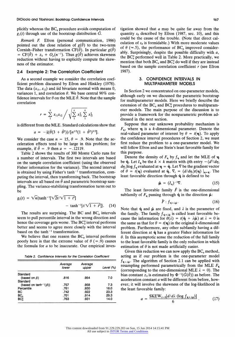
2.4 Example 2: The Correlation Coefficient

As a second example we consider the correlation coefficient problem discussed by Efron and Hinkley (1978). The data (xil, xi2) and iid bivariate normal with means 0, variances 1, and correlation 0. We base central 90% con-

A

fidence intervals for 0 on the MLE 0. Note that the sample correlation

n | n

r= 2 22>jxAx r=EXilXi2/i x2 Ei x22 1 1 1

is different from the MLE. Standard calculations show that

a = -X(0(3 + A2))/[n1/2(l + A2)3/2]

We consider the case n = 15, 0 = .9. Note that the acceleration effects tend to be large in this problem; for example, if 0 = .9 then a = -.12119.

Table 2 shows the results of 300 Monte Carlo runs for a number of intervals. The first two intervals are based on the sample correlation coefficient (using the observed Fisher information for the variance). The second interval is obtained by using Fisher's tanh-1 transformation, computing the interval, then transforming back. The bootstrap intervals are all based on 0 and parametric bootstrap sampling. The variance-stabilizing transformation turns out to be

gl(t) = \/ {tanh-1[V? t/VT72]

- tanh-[tI/'i77]}. (14)

The results are surprising. The BC and BCa intervals seem to pull percentile interval in the wrong direction and hence the coverage gets worse. The BCO interval performs better and seems to agree more closely with the interval based on the tanh-1 transformation.

We believe that one reason the BCa interval performs poorly here is that the extreme value of 0 (=.9) causes the formula for a to be inaccurate. Our empirical inves-

Table 2. Confidence Intervals for the Correlation Coefficient

Average Average lower upper Level (%/6)

Standard (based on p5) .816 .954 7.0

Standard (based on tanh-1(P)) .757 .958 7.3

Percentile .761 .930 18.0 BC .742 .922 23.3 BOa .701 .914 29.3 BC?a .763 .931 14.0

tigation showed that a may be quite far away from the quantity go described by Efron (1987, sec. 10), and this could be the cause of the trouble. (Note that direct calculation of eo is formidable.) With more moderate values of 0 ("-' .5), the performance of BCa improved consider- ably. Surprisingly, despite the possible difficulty with a, the BCO performed well in Table 2. More practically, we mention that both BCa and BCO do well if they are instead based on the sample correlation coefficient r (see Efron 1987).

3. CONFIDENCE INTERVALS IN MULTIPARAMETER MODELS

In Section 2 we concentrated on one-parameter models, although early on we discussed the parametric bootstrap for multiparameter models. Here we briefly describe the extension of the BCa and BCO procedures to multiparameter models. The main purpose of the discussion is to provide a framework for the nonparametric problem ad- dressed in the next section.

Suppose that our unknown probability mechanism is F., where q is a k-dimensional parameter. Denote the real-valued parameter of interest by 0 = t(11). To apply the confidence interval procedures of Section 2, we must first reduce the problem to a one-parameter model. We will follow Efron and use Stein's least favorable family for this purpose.

Denote the density of F. by f. and let the MLE of i be A. Let I, be the k x k matrix with ijth entry - (d2Id4li dij)log f, evaluated at a = . Let V be the gradient vector of 0 = t(q) evaluated at A, Vi = (dIdij)t(q) l The least favorable direction through A is defined to be

A= (I)1V. (15)

The least favorable family F is the one-dimensional subfamily of F., passing through a in the direction i:

Fi: f (16)

Note that A and Ai are fixed, and A is the parameter of the family. The family f,+Ar, is called least favorable because the information for 0(i) = t(i + AA) at A = O is the same as that for 0 = t(iq) in the original k-dimensional problem. Furthermore, any other subfamily having a different direction at A has a greater Fisher information for 0. In this asymptotic sense the reduction of the full family to the least favorable family is the only reduction in which estimation of 0 is not made artificially easier.

Given this reduction we can now apply the BCa method, acting as if our problem is the one-parameter model +f . The algorithm of Section 2.1 can be applied with resampling performed parametrically from the MLE F4 (corresponding to the one-dimensional MLE A = 0). The bias constant zo is estimated by G (0(O)) as before. The acceleration constant a will be different from before, however; it will involve the skewness of the log-likelihood in the least favorable family:

a = SKEWA=0[d/dA. (log f~+A')] . (17)




Except for some simple cases, estimation of a will require bootstrap computations. Fortunately, an explicit formula for a is available in the nonparametric case (next section).

Construction of the BC? interval follows that of Section 2. Here we use

g1(t) = [K2(S)p/2 ds

where Ki(s) is the expected Fisher information for A in the family f,4 A>, and ga(t) = (ea, - 1) la as before. Using (17) for a and zo = 4r-(GQ0)) we obtain an interval (AL, Av) for A. Finally, this gives an interval for 0 through the re- lationship 0() = t(i + AA ). Note that gl(t) will be difficult to calculate in general, but like a it is easily computed in the nonparametric case.

We have constructed the BCa and BCO intervals for multiparameter problems by extending the one-parameter definition to the least favorable family. To justify their use we need to show that in some sense they are second-order correct. It turns out that a correct interval is difficult to define; instead, we can require that each of the intervals err in their coverage only by Op(n-1). Formally,

Pr,(OBc [a] < 0 < BCa - a]) - 1 - 2a + OP(n-1) (18)

and similarly for OBco[a]. We conjecture this result and a also that

0BcoJ]-OB a aBt[a] - OBcaa] = Op(n1), (19)

but so far we have been unable to prove these conjectures.

4. NONPARAMETRIC PROBLEMS

If we were to approach the nonparametric problem in its most general form we would have to consider all possible distributions FX,; that is, let vj be infinite-dimensional. This would obviously be infeasible. Following Efron (1987), we simplify the problem substantially by assuming that F., has support only on the observed data xl, x2, . . ., x,. This makes the problem finite-dimensional, and the approach of Section 3 can be used.

Consider the data xl, x2, . . . , xn to be fixed and let ti = log(Pr(X = xi)), i = 1, 2, . . . , n. We can describe any realization from F,, by P*, where P =#Xk* = xi/ n. Then F. is a rescaled multinomial distribution; that is, P* - mult(n, e9)/n. The observed sample gives rise to ?q = log(P?), where P0 = (lln, 1/n, .. . , 1/n)' and hence FA = mult(n, P0)In. The least favorable family through a turns out to be P* mult(n, w')In, where wl = eluill eluW and

U, = lim s((1 -e)Fn + e&i) - t(Fn) (20)

(see Efron 1987, sec. 7). Here 5bi1S a point mass at xl, and the LJg are called the empirical influence components of 0 = s(Fn). In the notation of the previous section, ,hi = U-(U1, U2, ... ., Us)'. The Ui's are computed by sub-

stituting a small number like 1I(n + 1) for e in the right side of (20), except in the rare cases in which they can be calculated exactly.

We now have almost all we need to compute the BCa interval for the nonparametric case. Resampling is done from FX, = mult(n, PO)!n, and this is equivalent to sampling with replacement from x1, x2, . . . , x,. The bias constant is estimated by D-1(G (0)) as before. We require only an estimate of the acceleration a. Applying (17) to the multinomial family gives

a =(E u) )/6( u2) (21)

Table 1 (line 9) shows the results of the nonparametric BCa interval applied to the variance problem. The BCa interval outperforms the (nonparametric) percentile and bias-corrected percentile intervals but does not fully cap- ture the asymmetry of the exact interval. This is due to the short tails of the bootstrap distribution of 0.

To compute the BCO interval, we require an estimate of the expected Fisher information zcl(s) for A~ in the least favorable family. Straightforward calculations show that

n n 2

K2'(s) = n~ eU (ne j (22) E euis Eteuis

A simple numerical integration (like the trapezoid rule) is then used to compute g1(t). Note that (22) does not depend on the form of the statistic, just the Ui's, and hence the complexity of the statistic is not a problem. Note also that Kic(S) is a nonnegative function by Jensen's inequality, and hence g1(t) is monotone increasing and invertible.

Line 10 of Table 1 shows the results of the BCO procedure applied to the variance problem. As in the parametric case the results were very similar to the BCa results on an interval to interval basis.

Actually, computation of the BCO interval does not even require bootstrap sampling! The only component of the procedure that seems to require it is the estimation of zo. But Efron (1987, sec. 7) provided an alternative to (3) for zo based on first- and second-order empirical influences. Let V be the n x n matrix of second-order influences, define

n / n 3J2

Zoi= A 2 U [ i

(the approximation for a), and let

Z02 = [UtVU/11U112 - tr(V)]/(2nIIUI12).

Then a good approximation for zo is

zO:::- (T)-1(2(D(zo1)(D(Zo2))- (23)

Using the following method (due to Tim Hesterberg of Stanford), Z02 can be computed with only two additional evaluations of the statistic. Let U(i, e) equal the expression in the right side of (20) for some small positive e. Then it



DiCiccio and Tibshirani: Bootstrap Confidence Intervals 169

is easy to show that tr(V) (1/82) En U(i, e). Let D(i, e) = U(i, e) - U(c) = (1/n) En U(i, e). Using the notation ((P*) to denote 0 = s(F) evaluated for the distribution F putting mass Pi* onxi (see, e.g., Efron 1981), one can also show that

UWVU [L(PO + cU) + 0(P0 - gU) - 20(p0)]/g2

In summary, then, we compute U(1, e), U(2, e), . U(n, e), 0(P0 + cU), and 0(P0 - cU), and combine them to get estimates of z01, Z02, and hence z0. Therefore, a total of only n + 2 evaluations of the statistic are required to compute a and z0. We must remember, however, that (23) is only an approximation; Hesterberg is presently studying its accuracy.

Remark G. If the BCa and BC? intervals can be shown to be second-order correct, they will also be second-order correct in the nonparametric setting if it is assumed that the number of categories in the support of the multinomial stays fixed as n goes to infinity. Combined with the assumption that the support of the distribution is confined to x1, x2, . . . , x,, this is not an ideal definition of "nonparametric second-order correctness." We are currently considering ways of making it more realistic.

Remark H. The steps involved in computing the BC? interval are (a) calculation of z0 through formula (3) or (23), (b) calculation of a [formula (21)], (c) calculation of g1(t) through (22) and the trapezoid rule, to give g(t) from (10), and (d) inversion of g( ) to get an interval for A through (12). Finally, we get an interval for 0 through the relation 0(A) = t(i + )4Q). The BC? is therefore automatic in the same sense as the BCa interval; that is, it can be routinely applied to complicated statistics. But one poten- tial difficulty is present in this calculation: To compute (22) we must be able to compute our statistic for an arbitrary set of sample weights w1, w2, . . . , wn. A general but approximate way of doing this is to pick some large M such that Mwi is close to an integer for every i, then apply the statistic to a sample of size M with [Mwi] copies of xi (i = 1, 2, . . . , n). Often, however, we can avoid this by finding the equivalent weighted form of the problem (for an example see the next section). Note that this question does not arise with the BCa interval because it deals only with bootstrap samples.

Example 3: The Proportional Hazards Model

For illustration we apply these methods to the proportional hazards model of Cox (1972). The data we consider are the mouse leukemia data analyzed by Cox in that paper, which consist of the survival times (yi) in weeks of mice in two groups (xi), control (0) and treatment (1), as well as a censoring indicator (6i5). The proportional hazards model assumes that the hazard (or instantaneous probability of failing) in the treatment group is eA times the hazard in the control group. A standard analysis then pro- ceeds by maximizing the so-called partial likelihood over /3. In this case the partial likelihood estimator /3 is 1.51. We apply the confidence interval procedures by considering (y1, xi, 5si) as the sampling unit. We define the partial

Table 3. Confidence Intervals and Length for Proportional Hazards Example

Standard (.84, 2.18) [1.34] Percentile (.93, 2.34) [1.40] BC (.95, 2.36) [1.41] BC8 (.75, 2.15) [1.50] BCO (.87, 2.03) [1.16]

likelihood estimator for sample weights w, ,8(w), to max- imize

PL(w) = exp(> /xjxwj)

iED Ewi exp(xjf E WE ) (24) jER,

where D is the set of indexes of the failure times, Ri is the set of indexes of the items at risk before the ith failure, and each of the inner sums is over the items failing at the ith failure time (Tibshirani 1984). Formula (23) is used to compute zo. Table 3 shows the results of the various nonparametric confidence procedures, with a = .05. Inter- estingly, the percentile and BC intervals shift the standard interval to the right, but the negative acceleration (a = - .152) caused the BCa and BCO intervals to shift back to the left. The BCO is also somewhat shorter than the BCa interval.

5. APPROXIMATING THE BOOTSTRAP DISTRIBUTION OF A STATISTIC

The results of Sections 2 and 3 show (and conjecture), respectively, that

A ~~~~'Z0 + Z(a) G(ID(z[a])), za= z+1 - a(zo + Z(a)))

and -1 [ zo + Z(a) 1

gLi- az Z(a)) (25) differ by only Op(n-). We can use this to estimate G'(p) (for any p), without bootstrap sampling, as follows. First we find Z(a) such that p = D(z[a]); that is, Z(a) = (D-t1(p) - zo)/(l + aQ(t-1(p) - zo)) - zo. Then we substitute this into (25) and thus get an approximation to G -(p).

If instead we want a density that closely approximates the bootstrap histogram, we recall that

g(L) - g(O) - N(-zo(1 + g(O)), (1 + ag(0))2).

Hence a good approximating density is that of

9-1[g(O) - zo(1 + ag(O)) + Z(1 + ag(0))],

where Z is a N(O,1) random variable. Since g(O) = 0, this simplifies to g-'(Z - zo) and the resultant density works out to be

j(s) = 44(exp(g1(s)a) - 1)/a + zo]

x exp(g1(s)a)(K2(s))1"2, (26) where + is the density function of N(0,1). In the nonparametric case, (26) gives the density of A. and must be mul- tiplied by d)JdO = ni K2(s) to obtain the density for 0.




C\J

co

20.

6

C\1 ~ ~ r

0 1 2 3 4

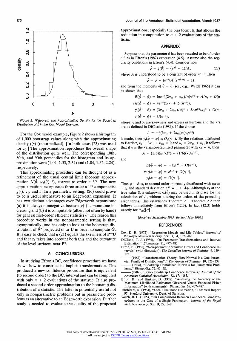
Figure 2. Histogram and Approximating Density for the Bootstrap Distribution of , in the Cox Model Example.

For the Cox model example, Figure 2 shows a histogram of 1,000 bootstrap values along with the approximating density j(s) (renormalized). [In both cases (23) was used for zo.] The approximation reproduces the overall shape of the distribution quite well. The corresponding 10th, 50th, and 90th percentiles for the histogram and its approximation were (1.04, 1.53, 2.34) and (1.04, 1.52, 2.24), respectively.

This approximating procedure can be thought of as a refinement of the usual central limit theorem approximation N(O, K2(O)1), correct to order n112. The new approximation incorporates three order n-1/2 components: g( ), zo, and a. In a parametric setting, (26) could prove to be a useful alternative to an Edgeworth expansion. It has two distinct advantages over Edgeworth expansions: (a) it is always nonnegative because g( ) is monotone increasing and (b) it is computable (albeit not often by hand) for general first-order efficient statistics 0. The reason this procedure works in the nonparametric setting is that, asymptotically, one has only to look at the bootstrap distribution of 0* projected onto U in order to compute G. It is easy to check that a (21) equals the skewness of P*'U and that zo takes into account both this and the curvature of the level surfaces near PO.

6. CONCLUSIONS

In studying Efron's BCa confidence procedure we have shown how to construct its implicit transformation. This produced a new confidence procedure that is equivalent (to second order) to the BCa interval and can be computed with only n + 2 evaluations of the statistic. It also produced a second-order approximation to the bootstrap distribution of a statistic. The latter is potentially useful not only in nonparametric problems but in parametric problems as an alternative to an Edgeworth expansion. Further study is needed to evaluate the quality of the proposed

approximations, especially the bias formula that allows the reduction in computation to n + 2 evaluations of the statistic.

APPENDIX

Suppose that the parameter 0 has been rescaled to be of order n1/2 as in Efron's (1987) expression (4.5). Assume also the regularity conditions in Efron's (4.4). Consider now

= g(0) = (eAO - 1)/A, (27) where A is understood to be a constant of order n-12. Then

q - = (eAO/A)(eA(66) - 1)

and from the moments of 0 - 0 (see, e.g., Welch 1965) it can be shown that

E(O - 4) = AneAO[(2K11 + K.,)/K 2n'2 + A/K2 + O(n var(q - 4) = ne2A0(lK2 + O(n 2)),

yi(o - 4) = (3K11 + 2K.1)/K32/2 + 3Anl/2 /K2 + O(n-1

Y2(0 - 4) = Q(n-1),

where y, and Y2 are skewness and excess in kurtosis and the K'S

are as defined in DiCiccio (1984). If the choice

A = -3(3K11 + 2KOo1)/(K2n 12)

is made, then yl( - 4) is O0(n-1). By the relations attributed to Bartlett, K3 + 3K11 + Kool = 0 and K3 = 2Ko01 + K', it follows that if 0 is the variance-stabilized parameter with K2 = n, then

A = (1/6)(K3/K3/2) = (1/6)(K3/n3/2),

and

E(O) - 4) = - zoeAO + O(n-1),

var(O - 4) = eA0 + 0(n-1),

Yi( - 4) = 0(n-1). Thus + - 4 is, to second order, normally distributed with mean - zo and standard deviation eAO = 1 + AO. Although K3 at the true value 00 is unknown, K3(0) may be used in its place for the calculation of A, without altering the orders of the preceding error terms. This establishes Theorem 2.1. Theorem 2.2 then follows immediately from Efron's (12.3). In fact (12.3) holds exactly for OBcja].

[Received September 1985. Revised May 1986.]

REFERENCES

Cox, D. R. (1972), "Regression Models and Life Tables," Journal of the Royal Statistical Society, Ser. B, 34, 187-202.

DiCiccio, T. J. (1984), "On Parameter Transformations and Interval Estimation," Biometrika, 71, 477-485.

Efron, B. (1981), "Non-parametric Standard Errors and Confidence In- tervals" (with discussion), The Canadian Journal of Statistics, 9, 139- 172.

(1982), "Transformation Theory: How Normal Is a One-Param- eter Family of Distributions?," The Annals of Statistics, 10, 323-339.

(1984), "Bootstrap Confidence Intervals for Parametric Prob- lems," Biometrika, 72, 45-58.

(1987), "Better Bootstrap Confidence Intervals," Journal of the American Statistical Association, 82, 171-185.

Efron, B., and Hinkley, D. (1978), "Assessing the Accuracy of the Maximum Likelihood Estimator: Observed Versus Expected Fisher Information" (with comments), Biometrika, 65, 457-487.

Tibshirani, R. (1984), "Local Likelihood Estimation," Technical Report 97, Stanford University, Dept. of Statistics.

Welch, B. L. (1965), "On Comparisons Between Confidence Point Pro- cedures in the Case of a Single Parameter," Journal of the Royal Statistical Society, Ser. B, 27, 1-8.



Documents

Bootstrap Confidence Intervals and Bootstrap Approximations