Embed Size (px)
Citation preview
Mach LearnDOI 10.1007/s10994-008-5065-7
Boosted Bayesian network classifiers
Yushi Jing · Vladimir Pavlovic · James M. Rehg
Received: 16 December 2005 / Revised: 21 November 2007 / Accepted: 5 May 2008Springer Science+Business Media, LLC 2008
Abstract The use of Bayesian networks for classification problems has received a signifi-cant amount of recent attention. Although computationally efficient, the standard maximumlikelihood learning method tends to be suboptimal due to the mismatch between its optimiza-tion criteria (data likelihood) and the actual goal of classification (label prediction accuracy).Recent approaches to optimizing classification performance during parameter or structurelearning show promise, but lack the favorable computational properties of maximum likeli-hood learning. In this paper we present boosted Bayesian network classifiers, a frameworkto combine discriminative data-weighting with generative training of intermediate models.We show that boosted Bayesian network classifiers encompass the basic generative modelsin isolation, but improve their classification performance when the model structure is subop-timal. We also demonstrate that structure learning is beneficial in the construction of boostedBayesian network classifiers. On a large suite of benchmark data-sets, this approach outper-forms generative graphical models such as naive Bayes and TAN in classification accuracy.Boosted Bayesian network classifiers have comparable or better performance in comparisonto other discriminatively trained graphical models including ELR and BNC. Furthermore,boosted Bayesian networks require significantly less training time than the ELR and BNCalgorithms.
Keywords Bayesian network classifiers · AdaBoost · Ensemble models · Structurelearning
Editor: Zoubin Ghahramani.
Y. Jing (�) · J.M. RehgCollege of Computing, Georgia Institute of Technology, Atlanta, GA 30332, USAe-mail: [email protected]
J.M. Rehge-mail: [email protected]
V. PavlovicDepartment of Computer Science, Rutgers University, Piscataway, NJ 08854, USAe-mail: [email protected]
Mach Learn
1 Introduction
A Bayesian network is an annotated directed graph that encodes the probabilistic relation-ships among variables of interest (Pearl 1988). The explicit representation of probabilisticrelations can exploit the structure of the problem domain, making it easier to incorporatedomain knowledge in the model design. In addition, a Bayesian network has a modular andintuitive graphical representation which is very beneficial in decomposing a large and com-plex problem representation into several smaller, self-contained models for tractability andefficiency. Furthermore, the probabilistic representation combines naturally with the EM al-gorithm to address problems with missing data. These advantages of Bayesian networks andgenerative models as a whole make them an attractive modeling choice.
In many problem domains where a Bayesian network is applicable and desirable, wemay want to infer the label(s) for a subset of the variables (class variables) given an instan-tiation of the rest (attributes). Bayesian network classifiers (Friedman et al. 1997) modelthe conditional distribution of the class variables given the attributes and predict the classwith the highest conditional probability. Bayesian network classifiers have been appliedsuccessfully in many application areas including computational molecular biology (Segalet al. 2003; Pavlovic et al. 2002; Jojic et al. 2004), computer vision (Torralba et al. 2004;Rehg et al. 2003; Schneiderman 2004), relational databases (Friedman et al. 1999), textprocessing (Cutting et al. 1992; McCallum et al. 2000; Lafferty et al. 2001), audio process-ing (Rabiner and Juang 1993) and sensor fusion (Pavlovic et al. 2000). Its simplest form, thenaive Bayes classifier, has received a significant amount of attention (Langley et al. 1992;Duda and Hart 1973; Ng and Jordan 2002).
However, standard Maximum Likelihood (ML) parameter learning in Bayesian net-work classifiers tends to be suboptimal (Friedman et al. 1997). It optimizes the jointlikelihood, rather than the conditional likelihood, a score more closely related to theclassification task. Unlike the joint likelihood, however, the conditional likelihood can-not be expressed in a log linear form, therefore no closed form solution is availableto compute the optimal parameters. Recently there has been substantial interest in dis-criminative training of generative models coupled with advances in discriminative opti-mization methods for complex probabilistic graphical models (Greiner and Zhou 2002;McCallum et al. 2000; Lafferty et al. 2001; Chelba and Acero 2004; Altun et al. 2003;Taskar et al. 2004).
If the selected model structure contains the structure from which the data is generated,the parameters that maximize the likelihood also maximize the conditional likelihood (seep. 5). For this reason, structure learning (Cooper and Herskovits 1992; Heckerman 1995;Friedman and Koller 2000; Chickering and Heckerman 1997; Heckerman et al. 1995; Lamand Bacchus 1992) can potentially be used to improve the classification accuracy. However,experiments show that learning an unrestricted Bayesian network fails to outperform naiveBayes in classification accuracy on a large sample of benchmark data (Friedman et al. 1997;Grossman and Domingos 2004). Friedman et al. (1997) attribute this to the mismatch be-tween the structure selection criteria (data likelihood) and the actual goal for classification(label prediction accuracy). They proposed Tree Augmented Naive Bayes (TAN), a struc-ture learning algorithm that learns a maximum spanning tree from the attributes, but incor-porates a naive Bayes model as part of its structure to bias the model towards the estima-tion of the conditional distribution. On the other hand, Keogh and Pazzani (1999) proposedAugmented Naive Bayes (ANC) algorithm that uses the 0-1 loss function as the optimiza-tion criteria in its heuristic search for the best k-tree Bayesian network classifiers. Recentlyproposed BNC-2P (Grossman and Domingos 2004) uses the conditional likelihood as opti-mization criteria in its structure search and is shown to outperform naive Bayes, TAN, and
Mach Learn
generatively trained unrestricted networks. Although the structures in TAN and BNC-2Pare selected discriminatively, the parameters are trained via ML training for computationalefficiency.
In this work, we propose a new approach to the discriminative training of Bayesian net-works. Similar to a standard boosting approach, we recursively form an ensemble of clas-sifiers. However in contrast to situations where the weak classifiers are trained discrim-inatively, the “weak classifiers” in our method are trained generatively to maximize thelikelihood of weighted data. Our approach has two benefits. First, ML training of genera-tive models is dramatically more efficient computationally than discriminative training. Bycombining maximum likelihood training with discriminative weighting of data, we obtain acomputationally efficient method for the discriminative training of a general Bayesian net-work. Second, our classifiers are constructed from generative models. This is important inmany practical problems where domain knowledge can be readily encoded in the structureof the generative model.
This paper makes five contributions:
1. We introduce Boosted Augmented Naive Bayes (bAN), an approach to improving theclassification accuracy of generative models. We demonstrate that bAN’s classificationaccuracy on a large suite of benchmark datasets is comparable or superior to competingmethods such as naive Bayes, TAN and ELR.
2. We investigate alternative training strategies for constructing boosted Bayesian networkclassifiers and introduce a novel algorithm bANmix as a more efficient alternative to bANdue to its heterogeneous assembly of structures.
3. We study the manner in which the complexity of the Bayesian network structure af-fects the classification accuracy of the final boosted ensemble by comparing bAN againstbBNC-2P, bTAN, and other alternative boosted Bayesian network classifiers. Our exper-iments highlight the importance of structure learning.
4. We demonstrate that bAN and bANmix are significantly faster to train than competingalgorithms including ELR and BNC-2P. To ensure fairness, we implemented bNB, bAN,TAN, BNC-2P, bTAN, bBNC-2P and ELR algorithms such that they share a commoncode base in C++. We optimized the common code base for efficiency. In addition, weoptimized the published BNC-2P method to improve its training speed.
5. We describe a multiclass extension of the bAN algorithm based on AdaBoost.MH andAdaBoost.M2. The results further demonstrate the advantages of structure selection.
A preliminary version of a portion of the results in this paper appeared in (Jing et al.2005). This paper differs from (Jing et al. 2005) in the following areas. We provide a de-tailed comparison against five alternative boosted Bayesian network learning algorithms todemonstrate that structure learning is crucial to the ensemble classification accuracy. We alsoinvestigate the effect of combining heterogeneous mixture of Bayesian network structuresinto one ensemble and propose bANmix as a more efficient alternative to bAN. We provideadditional experiments with simulated datasets (generated from more complex structures)to highlight the capability of bAN to explore the structure of the data distribution. We sup-plement the analysis of training cost in (Jing et al. 2005) with a thorough empirical eval-uations and comparisons (Sect. 7, Fig. 9 to Fig. 11). We include both AdaBoost.MH andAdaBoost.M2 variations in our analysis of multi-class bAN algorithm. Finally, we providea graphical interpretation of boosted Bayesian network classifier in Fig. 12 in the appendix.
This paper is divided into 8 sections. Sections 1 through 3 review the formal notations ofBayesian networks and parameter learning methodologies. Section 4 introduces AdaBoostas an effective way to improve the classification accuracy of naive Bayes. Section 5 ex-tends this work to structure learning and proposes the bAN and bANmix structure learning
Mach Learn
algorithm. Sections 6 and 7 contain the experiments and analysis for boosted naive Bayes,bAN and bANmix structure learning algorithm. The last three sections contain related works,conclusions and acknowledgments.
2 Bayesian Network Classifier
A Bayesian network B is a directed acyclic graph that encodes a joint probability distributionover a set of random variables X = {X1,X2, . . . ,XN } (Pearl 1988). It is defined by the pairB = {G,θ}. G is the structure of the Bayesian network. θ is the vector of parameters thatquantifies the probabilistic model. B represents a joint distribution PB(X), factored over thestructure of the network where
PB(X) =N∏
i=1
PB(Xi |Pa(Xi)) =N∏
i=1
θXi |Pa(Xi ).
We set θxi |Pa(xi ) equal to PB(xi |Pa(xi)) for each possible value of Xi and each possible in-stantiation of the parent of Xi , Pa(Xi).1 For notational simplicity, we define a one-to-onerelationship between the parameter θ and the entries in the local Conditional ProbabilityTable. Given a set of i.i.d. training data D = {x1, x2, x3, . . . , xM}, the goal of learning aBayesian network B is to find a {G,θ} that accurately models the distribution of the data.The selection of θ is known as parameter learning and the selection of G is known as struc-ture learning.
The goal of a Bayesian network classifier is to correctly predict the label for class Xc ∈ Xgiven a vector of attributes Xa = X\Xc. A Bayesian network classifier models the jointdistribution P (Xc,Xa) and converts it to conditional distribution P (Xc|Xa). Prediction forXc can be obtained by applying an estimator to the conditional distribution. For example,Maximum a Posteriori estimator (MAP) can be used to select the label associated with thehighest conditional probability.
3 Parameter learning
The Maximum Likelihood (ML) method is one of the most commonly used parameter learn-ing techniques. It chooses the parameter values that maximize the Log Likelihood (LL)score, a measure of how well the model represents the data. Given a set of training dataD with M samples and a Bayesian Network structure G with N nodes, the LL score isdecomposed as:
LLG(θ |D) =M∑
j=1
logPθ(Dj ) =
M∑
j=1
N∑
i=1
log θxji|pa(xi )
j
1We use capital letters to represent random variable(s) and lowercase letters to represent their correspondinginstantiations. Subscripts are used as variable indices and superscripts are used to index the training data.Pa(Xi) represents the parent node of Xi , pa(Xi) represents an instantiation of Pa(Xi) and pa(Xi)
j is theinstantiated value of Pa(Xi) in the j -th training data. In this paper, we assume all of the variables are discreteand fully observed in the training data.
Mach Learn
= M
N∑
i=1
∑
xi∈Xipa(xi )∈Pa(xi )
PD(xi,pa(xi)) log θxi |pa(xi ). (1)
LLG(θ |D) is maximized by simply setting each parameter θxi |Pa(xi ) to PD(xi |Pa(xi)),the empirical distribution of the data D. For this reason, ML parameter learning is compu-tationally efficient and very fast in practice.
However, the goal of a classifier is to accurately predict the label given the attributes,a function that is directly tied to the estimation of the conditional likelihood. Instead ofmaximizing the LL score, we would prefer to maximize the Conditional Log Likelihood(CLL) score. As pointed out in (Friedman et al. 1997), the LL score factors as
LLG(θ |D) = CLLG(θ |D) +M∑
j=1
logPθ(xja ),
where
CLLG(θ |D) =M∑
j=1
logPθ(xic |x j
a ) (2)
= M∑
xa∈Xaxc∈Xc
PD(xc, xa) logPθ(xc|xa). (3)
Given a network structure G that encapsulates the true structure of the data, parameters thatmaximize LLG also maximize CLLG.2 However, in practice the structure may be incorrectand ML learning will not optimize the CLL score, which can result in a suboptimal classifi-cation decision.3
An alternative approach is to directly optimize Eq. 3, which is maximized when
Pθ(xc|xa) = θxc
∏θxa |Pa(xa)∑
xcθxc
∏θxa |Pa(xa)
= PD(xc|xa). (4)
For a generative model such as a Bayesian network, Eq. 4 cannot be expressed in log-linearform and has no closed form solution. A direct optimization approach requires computation-ally expensive numerical techniques. For example, the ELR method of (Greiner and Zhou2002) uses gradient descent and line search to directly maximize the CLL score. However,this approach is unattractive in the presence of a large feature space, especially when usedin conjunction with structure learning.
2The asymptotic properties of likelihood and conditional likelihood learning is discussed in greater detailin (Nadas 1983).3If G is incorrect, maximizing CLLG may also lead to poor performance. However, LL score is more sensitivethan CLL since it requires correct knowledge of the features (Devroye et al. 1996).
Mach Learn
4 Boosted parameter learning
4.1 Ensemble model
Instead of maximizing the CLL score for a single Bayesian network model, we take theensemble approach and maximize the classification performance of the ensemble Bayesiannetwork classifier. For binary classification, given a class xc and the attributes xa , an ensem-ble model has the general form:
Fxc (xa) =K∑
k=1
βkfk,xc (xa). (4.1)
and fk,xc (xa) is the classifier confidence on selecting label xc given xa during boosting it-eration k, and βk is its corresponding weight. In the case where xc ∈ {−1,1}, fk,xc (xa) istypically defined as the following: fk,xc (xa) = xcfk(xa), where fk(xa) ∈ {−1,1} is the out-put of each classifier given xa , and F(xa) is the ensemble of f (xa). Equation 4.1 can beexpressed as a conditional probability distribution over Xc given the additive model F withlogistic transformation:
PF (xc|xa) = exp{Fxc (xa)}∑x′c∈Xc
exp{Fx′c(xa)} . (5)
For binary classification, Eq. 5 is then updated as:
PF (xc|xa) = 1
1 + exp{−2xcF (xa)} . (6)
Instead of directly optimizing CLL, we minimize the often used Exponential Loss Function(ELF) of the ensemble Bayesian network classifier. ELF is defined as:
ELFF =M∑
i=1
exp{−x ic F (x i
a )}. (7)
Solving for xcF (xa) in Eq. 6 and combining with Eq. 7, we have
ELFF =M∑
i=1
exp
{1
2log
1 − PF (x ic |x i
a )
PF (x ic |x i
a )
}(8)
= M∑
xa∈Xaxc∈Xc
PD(xc, xa)
√1
PF (xc, xa)− 1. (9)
Equation 9 is a differentiable upper bound on the classification error, and an approximationto the negative CLL score (Friedman et al. 2000).4
4The ELF criteria has been demonstrated to be an effective classification error minimization criteria, and toperform well on real data. A detailed comparison of ELR and CLL can be found in (Friedman et al. 2000).
Mach Learn
Table 1 Boosted parameter learning algorithm
1. Given a base structure G and the training data D, where M is the number of training cases.
D = {x 1c x 1
a , x 2c x 2
a , . . . , x Mc x M
a } and xc ∈ {−1,1}.2. Initialize training data weights with wi = 1/M, i = 1,2, . . . ,M
3. Repeat for k = 1,2, . . .
• Given G, θk is learned through ML parameter learning on the weighted data Dk .
• Compute the weighted error, Errk = Ew[1xc �=fθk(xa)], βk = 0.5 log 1−Errk
Errk.
• Update weights wi = wi exp{−βkx ic f (x i
a | θk,Gk)} and normalize.
4. Ensemble output: sign∑
k βkf (xa | θk,Gk)
4.2 Boosted parameter learning
An ensemble Bayesian network classifier takes the form Fθ,β where θ is a collection ofparameters in the Bayesian network model and β is the vector of hypothesis weights. Wewant to minimize ELFθ,β of the ensemble Bayesian network classifier as an alternative wayto maximize the CLL score. We used Discrete AdaBoost algorithm, which is proven togreedily and approximately minimize the exponential loss function in Eq. 9 (Friedman et al.2000).
At k-th iteration of boosting, the weighted data uniquely determines the parameters foreach Bayesian network classifier θk and the hypothesis weights βk via efficient ML parame-ter learning, where
βk = 0.5 log1 − Errk
Errk
, θk(xa|xc) = PDk(xa|xc) (10)
where Errk is the classification error on the weighted data. The full algorithm is shown inTable 1. There is no guarantee that AdaBoost will find the global minimum of the ELF.Also, AdaBoost has been shown to be susceptible to label noise (Dietterich 2000; Bauer andKohavi 1999). In spite of these issues, boosted classifiers tend to produce excellent results inpractice (Schapire and Singer 2000; Drucker and Cortes 1996). Boosted Naive Bayes (bNB)has been previously shown to improve the classification accuracy of naive Bayes (Elkan1997; Ridgeway et al. 1998).
5 Structure learning
Given training data D, structure learning is the task of finding a set of directed edges G thatbest model the true density of the data. In order to avoid overfitting, Bayesian Scoring Func-tion (Cooper and Herskovits 1992; Heckerman et al. 1995) and Minimal Description Length(MDL) (Lam and Bacchus 1992) are commonly used to evaluate candidate structures. TheMDL score is asymptotically equivalent to the Bayesian scoring function in the large samplecase and this paper will concentrate on the MDL score. MDL score is defined as
MDL(B|D) = log |D|2
|B| − LL(B|D) (11)
where |B| is the total number of parameters in model B , and |D| is the total number oftraining samples.
Mach Learn
Table 2 Boosted augmented naive Bayes (bAN)
1. Given training data D, construct a complete graph Gf ull with attributes Xa as vertices.
Calculate Ip(Xai;Xaj
|Xc) for each pair of attributes Xa , i �= j , where
Ip(Xai;Xaj
|Xc) =∑
xai∈Xai
xaj∈Xaj
,xc∈Xc
P (xai, xaj
, xc) logP(xai
, xaj|xc)
P (xai|xc)P (xaj
|xc)(12)
2. Construct GT AN from Gf ull with Ip as weights, set G1 = naive Bayes.
3. For s = 1 to N − 1
• Parameter boosting using Gs as base structure.
• Evaluate the classification accuracy for the current GbAN on training data D, and terminate if it
stops decreasing.
• Else, remove the edge {XaiXaj
} containing the largest conditional mutual information
Ip(Xai;Xaj
|Xc) from GT AN and add it to Gs .
• Gs+1 = Gs .
4. Ensemble output: sign∑K
k=1 βkf (xa | θk,Gs), where K is the number of classifiers in the ensemble
with Gs as base structure.
An exhaustive search over all structures against an evaluation function can in principlefind the best Bayesian network model, but in practice, since the structure space is super ex-ponential in the number of variables in the graph, it is not feasible in nontrivial networks.Several tractable heuristic approaches have been proposed to limit the search space. The al-gorithms K2 (Cooper and Herskovits 1992) and MCMC-K2 (Friedman and Koller 2000)define a node ordering such that a directed edge can only be added from a high rank-ing node to a low ranking node. Heckerman et al. (1995) proposed a hill-climbing localsearch algorithm to incrementally add, remove or reverse an edge until a local optimum isreached.
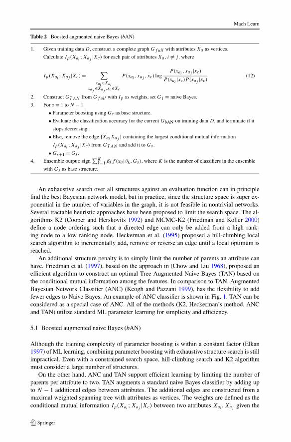
An additional structure penalty is to simply limit the number of parents an attribute canhave. Friedman et al. (1997), based on the approach in (Chow and Liu 1968), proposed anefficient algorithm to construct an optimal Tree Augmented Naive Bayes (TAN) based onthe conditional mutual information among the features. In comparison to TAN, AugmentedBayesian Network Classifier (ANC) (Keogh and Pazzani 1999), has the flexibility to addfewer edges to Naive Bayes. An example of ANC classifier is shown in Fig. 1. TAN can beconsidered as a special case of ANC. All of the methods (K2, Heckerman’s method, ANCand TAN) utilize standard ML parameter learning for simplicity and efficiency.
5.1 Boosted augmented naive Bayes (bAN)
Although the training complexity of parameter boosting is within a constant factor (Elkan1997) of ML learning, combining parameter boosting with exhaustive structure search is stillimpractical. Even with a constrained search space, hill-climbing search and K2 algorithmmust consider a large number of structures.
On the other hand, ANC and TAN support efficient learning by limiting the number ofparents per attribute to two. TAN augments a standard naive Bayes classifier by adding upto N − 1 additional edges between attributes. The additional edges are constructed from amaximal weighted spanning tree with attributes as vertices. The weights are defined as theconditional mutual information Ip(Xai
;Xaj|Xc) between two attributes Xai
,Xajgiven the
Mach Learn
Fig. 1 An example of ANC, thedotted edges are structuralextensions to naive Bayes
class node Xc where
Ip(Xai;Xaj
|Xc) =∑
xc∈Xcxai
∈Xaixaj
∈Xaj
P (xai, xaj
, xc) logP (xai
, xaj|xc)
P (xai|xc)P (xaj
|xc).
TAN learning algorithm constructs the optimal tree-augmented network BT that maxi-mizes LL(BT |D). However, the TAN model adds a fixed number of edges regardless of thedistribution of the training data. If we can find a simpler model to describe the underlyingconditional distribution, then there is usually less chance of over-fitting.
Our bAN learning algorithm extends the TAN approach using parameter boosting. Start-ing from a naive Bayes model, at iteration s, bAN greedily augments the current structurewith the s-th edge having the highest conditional mutual information. We call the result-ing structure bANs . We then minimize the ELF score of the bANs classifier with parameterboosting. bAN terminates when the added edge does not improve the classification accu-racy of the training data. Since TAN contains N − 1 augmenting edges, bAN in worst caseevaluates N − 1 structures. This complexity is linear in N , in comparison to the polyno-mial number of structures examined by K2 or Hill-Climbing algorithms. Moreover, we findthat in practice (as shown in Table 4) that bAN usually only adds a small number of edgesto naive Bayes, significantly fewer than the competing algorithms like TAN, BNC-2P andBNC-MDL. As a result, the base Bayesian network structure constructed from bAN usuallycontains fewer edges than other competing structure learning algorithms, making it compu-tationally very efficient. The algorithm is shown in Table 2.
5.2 Boosted augmented naive Bayes with heterogeneous mixture of structures (bANmix )
The bAN learning algorithm constrains all weak classifiers to share a homogeneous struc-ture. In our previous work (Jing et al. 2005), this constraint was chosen partially to facilitatecomparison with other Bayesian network classifiers. As a result, structure selection can beseen as a wrapper function to the parameter boosting.
This section explores techniques in learning an ensemble Bayesian network classifierwith heterogeneous structures. Choudhury et al. (2002) explored the idea of combining there-weighting of training data with structure selection during each iteration of boosting fordynamic Bayesian networks.
In our work, we employ the greedy strategy of incrementally adding edges to the basestructure during iterations of boosting. The greedy structure learning algorithm, named
Mach Learn
bANmix , starts by constructing a TAN structure similar to the one proposed in bAN. We sortthe edges in TAN based on their conditional mutual information in descending order. Start-ing with naive Bayes, we apply parameter boosting on the initial structure until the weightederror is higher than ε.5 This step is analogous to the first step of bAN (up to S = 1). Next,we augment the current structure with the next “best” edge from TAN. However, instead ofrestarting a new round of parameter boosting with a new structure, we retain the ensemblegenerated so far, but train the new and more complex structure on the re-weighted data. Theaddition of a more complex structure, by better capturing the underlying distribution of thedata, usually reduces the weighted error and allows boosting to continue. We iterate thisprocess until the new structure does not improve the classification accuracy. In effect, weare incrementally generating an ensemble of sparsely connected, heterogeneous mixture ofBayesian network classifiers. The psudocode for bANmix is shown in Table 3.
There are two basic strategies that underly the bANmix algorithm. First, in order to avoidoverfitting, we select edges parsimoniously to maintain the sparsity of our generativelytrained Bayesian network classifiers. An edge is added to the structure only when the ex-isting weak classifier can no longer effectively classify the weighted samples. Our secondstrategy is to add edges with the highest conditional mutual information from TAN, underthe assumption that those edges, by capturing the most important relationship informationin the data, have the most potential to contribute to the classification accuracy.
To assess the effectiveness of these two strategies, we formulated two alternative train-ing algorithms. The first algorithm, bANmix(1), tests the first strategy. Rather than waitingfor boosting to converge, bANmix(1) adds a new edge to the existing structure at each itera-tion of boosting. Therefore, each structure is used exactly once (hence the name bANmix(1)).bANmix(1) terminates when the classification accuracy does not improve, or when the max-imum number of edges have been added. The second algorithm, bANmix(r), tests a randomstructure selection strategy. Instead of selecting the edge with the best conditional mutual in-formation from TAN, it randomly selects an edge from TAN to add to the existing Bayesiannetwork. The next two sections provide a detailed analysis of these three algorithms anddemonstrate that bANmix outperforms bANmix(1), bANmix(r) and has comparable perfor-mance to bAN. However, bANmix is more efficient to train than bAN.
We also implemented the MCMC variation of K2 from Friedman and Koller (2000)to study the effect of combining structure optimization with parameter boosting. K2 is agreedy search algorithm which uses a known ordering of the nodes and a maximum limit onthe number of parents for any node to constrain the search, and the MCMC variant samplesfrom the space of node orderings. As we show in Sect. 6, in spite of its tremendous compu-tational cost, MCMC K2 did not yield superior classification accuracy than bANmix , furtherconfirming the observation by Grossman and Domingos (2004) that exhaustive structure op-timization offers little classification improvement when combined with discriminative para-meter learning.
6 Experiments
We evaluated the performance of bNB and variations of bAN on 23 datasets from the UCIrepository (Blake and Merz 1998) and two artificial data sets, Corral and Mofn, designedby Kohavi and John (1997). Friedman et al. (1997), Greiner and Zhou (2002), Grossman
5We use ε = 0.45 in our experiments as the stopping criterion to reduce the number of model boosting rounds.No significant change in accuracy was observed compared to ε = 0.50.
Mach Learn
Table 3 Boosted augmented naive Bayes with mixed structure
1. Given a base structure G and the training data D, where M is the number of training cases.
D = {x 1c x 1
a , x 2c x 2
a , . . . , x Mc x M
a } and xc ∈ {−1,1}.2. construct a complete graph Gf ull with attributes Xa as vertices. Calculate Ip(Xai
;Xaj|Xc) for each
pair of attributes Xa , i �= j , where
Ip(Xai;Xaj
|Xc) =∑
xai∈Xai
xaj∈Xaj
,xc∈Xc
P (xai, xaj
, xc) logP(xai
, xaj|xc)
P (xai|xc)P (xaj
|xc)(13)
3. Construct GT AN from Gf ull with Ip as weights.
4. Initialize the training data weights with wi = 1/M, i = 1,2, . . . ,M
5. Set the initial Bayesian network structure as G1 = naive Bayes, and GbANmix= {}.
6. Repeat for k = 1,2, . . .
• Given Gk , θk is learned through ML parameter learning on the weighted data D at iteration k.
• Compute the weighted error, Errw(Gk) = Ew[1xc �=fθk(xa)], βk = 0.5 log 1−Errw(Gk)
Errw(Gk).
• GbANmix= {GbANmix
, Gk}
• If Errw(Gk) ≤ ε, update weights wi = wi exp{−βkx ic fθk
(x ia )} and normalize.
• Else, if Err(GbANmix) calculated from the training data D remains the same, terminate the loop;
or remove the edge with the highest Ip(Xai;Xaj
|Xc) from GT AN and add to Gk .
• Set Gk+1 = Gk .
7. Ensemble output: sign∑
k βkf (xa |θk,Gk)
and Domingos (2004) and Pernkopf and Bilmes (2005) used this group of data sets asbenchmarks for Bayesian network classifiers. We used hold-out test for larger data setsand 5 fold cross validation for smaller sets.6 To ensure fairness, we used Dirichlet priorBayesian smoothing, with parameters identical to the ones from page 18 of Friedman etal. (1997) for all classifiers when appropriate. The data preparation, experimental set-up aswell as Bayesian smoothing are the same as those used by Friedman et al. for the evaluationof TAN (Friedman 1997). Since the Wilcoxon Signed-Ranks Test is demonstrated to pro-vide the most unbiased evaluations for comparing methods across multiple datasets (Dem-sar 2006), we also used it to generate confidence scores. All algorithms are implemented inC++.7
The abbreviations for competing algorithms are described below:
• bANMH , bANM2: Boosted Augmented Naive Bayes trained via AdaBoost.MH and Ad-aBoost.M2 algorithm respectively.
• NB: Naive Bayes.• TAN: Tree Augmented naive Bayes (Friedman et al. 1997).• BNC-2P: Discriminative structure selection via CLL score (Grossman and Domingos
2004).• ELRNB , ELRT AN : NB and TAN with parameters optimized for conditional log likeli-
hood as in Greiner and Zhou (2002).
6We used hold-out test for “chess”, “letter”, “mofn”, “satimage”, “segment”, “shuttle”, “waveform,” and5 folds cross validation for the rest. We removed the data points with missing values and used pre-discretization step in manner described by Dougherty et al. (1995).7The C++ code can be found at www.cc.gatech.edu/cpl/projects/boosted_bnc.html.
Mach Learn
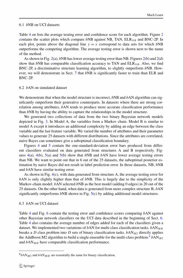
6.1 bNB on UCI datasets
Table 4 on lists the average testing error and confidence score for each algorithm. Figure 2contains the scatter plots which compare bNB against NB, TAN, ELRNB and BNC-2P. Ineach plot, points above the diagonal line y = x correspond to data sets for which bNBoutperforms the competing algorithm. The average testing error is shown next to the nameof the method.
As shown in Fig. 2(a), bNB has lower average testing error than NB. Figures 2(b) and 2(d)show that bNB has comparable classification accuracy to TAN and ELRNB . Also, we findBNC-2P, a discriminative structure learning algorithm, to slightly outperform bNB. How-ever, we will demonstrate in Sect. 7 that bNB is significantly faster to train than ELR andBNC-2P.
6.2 bAN on simulated dataset
We demonstrate that when the model structure is incorrect, bNB and bAN algorithm can sig-nificantly outperform their generative counterparts. In datasets where there are strong cor-relation among attributes, bAN tends to produce more accurate classification performancethan bNB by having the ability to capture the relationships in the model structure.
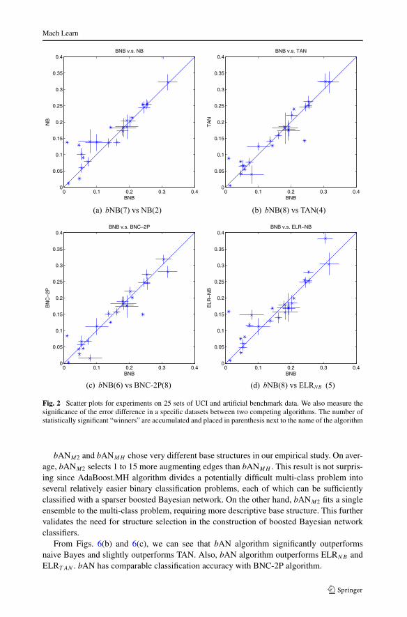
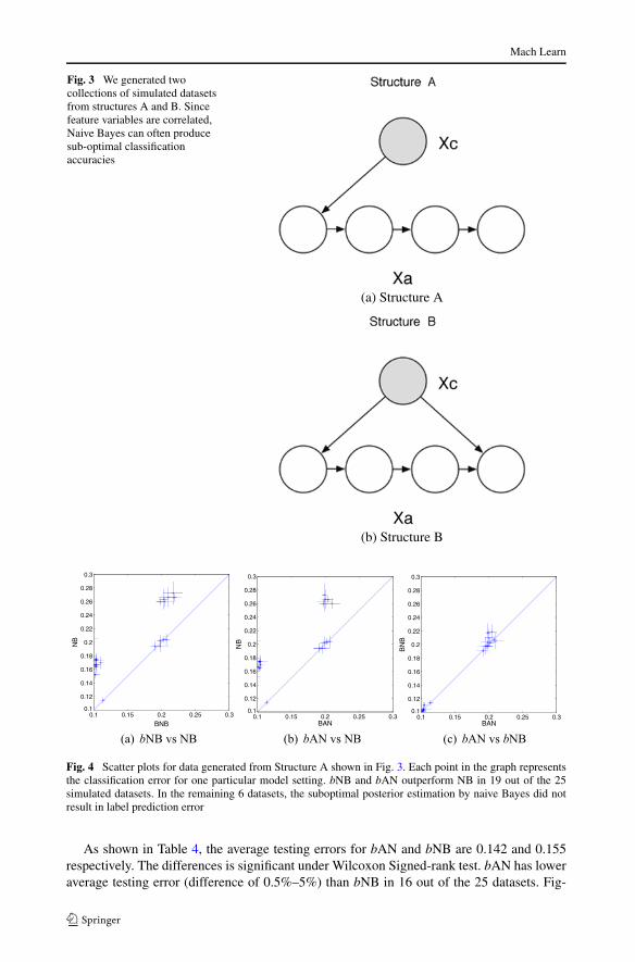
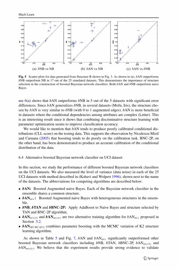
We generated two collections of data from the two binary Bayesian network modelsdepicted in Fig. 3. In Model A, the variables form a Markov chain. Model B is similar tomodel A except it introduces an additional complexity by adding an edge between the classvariable and the last feature variable. We varied the number of attributes and their parametervalues to generate 25 datasets with different distributions. Since the attributes are correlated,naive Bayes can sometimes give a suboptimal classification boundary.
Figures 4 and 5 contain the one-standard-deviation error bars produced from differ-ent classifiers evaluated on data generated from structures A and B respectively. Fig-ures 4(a), 4(b), 5(a) and 5(b) show that bNB and bAN have lower average testing errorsthan NB. We want to point out that in 6 out of the 25 datasets, the suboptimal posterior es-timation by naive Bayes did not result in label prediction error. In those datasets, NB, bNBand bAN have similar testing error.
As shown in Fig. 4(c), with data generated from structure A, the average testing error forbAN is only slightly higher than that of bNB. This is largely due to the simplicity of theMarkov-chain model: bAN selected bNB as the best model (adding 0 edges) in 20 out of the25 datasets. On the other hand, when data is generated from more complex structure B, bANsignificantly outperforms bNB shown in Fig. 5(c) by adding additional model structures.
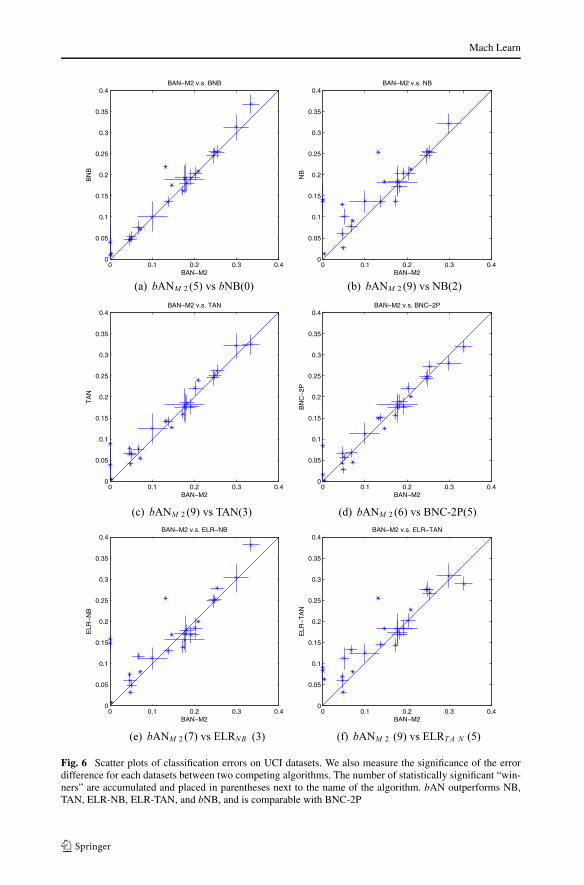
6.3 bAN on UCI dataset
Table 4 and Fig. 6 contain the testing error and confidence scores comparing bAN againstother Bayesian network classifiers on the UCI data described in the beginning of Sect. 6.Table 4 also contains the average number of edges added for each of the classifiers given adataset. We implemented two variations of bAN for multi-class classification tasks. bANMH
breaks a D class problem into D sets of binary classification tasks. bANM2 directly appliesthe AdaBoost.M2 algorithm to build a single ensemble for the multi-class problem.8 bANM2
and bANMH have comparable classification performance.
8bANM2 and bANMH are essentially the same for binary classification.

Mach Learn
Tabl
e4
Test
ing
erro
rsan
dits
asso
ciat
edco
nfide
nce
scor
esco
mpa
ring
two
clas
sifie
rson
mul
tiple
data
sets
.We
also
incl
uded
the
tota
lnum
bero
fedg
esad
ded
tofin
alA
Nst
ruct
ure,
aver
aged
over
diff
eren
tev
alua
tion
fold
s.W
ilcox
onSi
gned
-Ran
ksTe
stan
dFr
iedm
anTe
stw
ithpo
st-h
ocB
onfe
rron
ite
star
eus
edto
gene
rate
confi
denc
esc
ores
.“*
”in
dica
tes
data
sets
with
bina
rycl
ass
vari
able
s,w
here
bAN
MH
and
bAN
M2
prod
uce
the
sam
ecl
assi
ficat
ion
accu
racy
.“⇐
”in
dica
tes
the
case
sw
here
bAN
M2
stat
istic
ally
sign
ifica
ntly
outp
erfo
rms
the
com
petin
gm
odel
(acc
ordi
ngto
the
corr
espo
ndin
gte
st).
We
also
incl
uded
the
num
ber
ofau
gmen
ted
edge
sfo
rea
chB
ayes
ian
netw
ork
clas
sifie
r.(B
yde
finiti
on,
naiv
eB
ayes
and
EL
RN
Bco
ntai
ns0
augm
ente
ded
ges.
TAN
and
EL
RT
AN
cont
ains
N−
1nu
mbe
rof
augm
ente
ded
ges,
whe
reN
isth
enu
mbe
rof
feat
ures
inth
eda
tase
ts.W
hen
5-fo
ldcr
oss
valid
atio
nis
used
,we
aver
aged
the
num
ber
ofau
gmen
ted
edge
s)
Nam
ebA
NM
2/#
edge
sbA
NM
H/#
edge
sbN
BN
BTA
N/#
edge
sB
NC
-2P
/#ed
ges
EL
RN
BE
LR
TA
N
aust
ralia
n0.
1725
/0.4
*0.
1623
0.13
770.
1594
/13
0.15
65/1
1.5
0.13
910.
1435
brea
st0.
0483
/1.0
*0.
0469
0.02
640.
0412
/9.0
0.02
78/7
.00.
0322
0.03
22
ches
s0.
0460
/0.0
*0.
0460
0.12
950.
0788
/35
0.04
32/3
20.
0750
0.06
86
clev
e0.
1825
/0.8
*0.
1792
0.17
240.
1858
/12
0.18
93/9
.00.
1710
0.16
89
corr
al0.
0000
/1.0
*0.
1240
0.14
120.
0394
/5.0
0.01
57/3
.50.
1483
0.08
25
crx
0.13
78/0
.4*
0.13
620.
1362
0.14
24/1
40.
1516
/11
0.13
810.
1454
diab
etes
0.24
87/0
.8*
0.25
520.
2552
0.25
13/7
.00.
2448
/5.0
0.25
260.
2760
flare
0.19
14/2
.0*
0.19
320.
2035
0.17
73/9
.00.
1782
/9.0
0.16
790.
1838
germ
an0.
2540
/1.6
*0.
2540
0.25
400.
2620
/19
0.27
20/1
60.
2790
0.26
70
glas
s0.
2990
/1.2
0.29
89/0
.60.
3130
0.32
210.
3221
/8.0
0.28
04/4
.00.
3040
0.30
82
glas
s20.
2023
/0.0
*0.
2023
0.20
230.
2208
/8.0
0.22
08/7
.00.
1843
0.20
25
hear
t0.
1778
/1.0
*0.
1926
0.18
520.
1741
/12
0.17
41/1
00.
1764
0.17
41
hepa
titis
0.10
00/0
.0*
0.10
000.
1375
0.12
50/1
80.
1125
/16
0.11
250.
1250
iris
0.04
67/0
.20.
0533
/0.0
0.04
670.
0600
0.06
67/3
.00.
0667
/3.0
0.06
000.
0600
lette
r0.
1316
/13
0.18
58/3
.00.
2194
0.25
340.
1428
/15
0.14
96/1
10.
2550
0.25
50
lym
phog
raph
y0.
1765
/1.4
0.18
30/1
.00.
1897
0.18
270.
1810
/17
0.18
28/1
40.
1563
0.18
34
mof
n-3-
7-10
0.00
00/1
.0*
0.00
960.
1377
0.08
89/9
.00.
0840
/8.5
0.15
420.
0898
pim
a0.
2449
/1.0
*0.
2449
0.24
490.
2461
/7.0
0.24
74/6
.50.
2487
0.27
61
satim
age
0.14
65/1
50.
1425
/1.0
0.17
500.
1835
0.12
75/3
50.
1255
/32
0.16
850.
1830
segm
ent
0.07
14/1
.00.
0584
/0.0
0.07
140.
0909
0.05
45/1
80.
0455
/17
0.08
050.
0805
shut
tle-s
mal
l0.
0036
/2.0
0.00
62/2
.00.
0124
0.01
240.
0047
/8.0
0.00
20/8
.00.
0078
0.06
26

Mach Learn
Tabl
e4
(Con
tinu
ed)
Nam
ebA
NM
2/#
edge
sbA
NM
H/#
edge
sbN
BN
BTA
N/#
edge
sB
NC
-2P
/#ed
ges
EL
RN
BE
LR
TA
N
soyb
ean-
larg
e0.
0676
/1.6
0.08
00/1
.60.
0747
0.07
830.
0765
/34
0.06
75/3
00.
1174
0.13
28
vehi
cle
0.33
41/3
.80.
3120
/3.8
0.36
750.
4101
0.32
49/1
70.
3191
/15
0.38
170.
2894
vote
0.05
06/0
.6*
0.05
290.
1011
0.06
44/1
50.
0575
/14
0.04
830.
1126
wav
efor
m0.
2087
/1.0
0.21
21/1
.00.
2087
0.21
320.
2396
/20
0.20
11/1
80.
1996
0.22
74
Ave
rage
0.14
17/(
2.04
)0.
1436
/(1.
03)
0.15
510.
1709
0.15
19/(
14.6
8)0.
1446
/(12
.72)
0.16
230.
1652
bAN
MH
bNB
NB
TAN
BN
C-2
PE
LR
NB
EL
RT
AN
Wilc
oxon
SRte
stbA
NM
2⇐
−2.7
71⇐
−3.8
61⇐
−3.6
19⇐
−1.9
24⇐
−2.8
93⇐
−3.8
07
Frie
dman
/Bon
ferr
onit
est
bAN
M2
⇐−2
.13
⇐−2
.91
⇐−1
.96
−0.2
8⇐
−1.6
6⇐
−3.2
0
Mach Learn
Fig. 2 Scatter plots for experiments on 25 sets of UCI and artificial benchmark data. We also measure thesignificance of the error difference in a specific datasets between two competing algorithms. The number ofstatistically significant “winners” are accumulated and placed in parenthesis next to the name of the algorithm
bANM2 and bANMH chose very different base structures in our empirical study. On aver-age, bANM2 selects 1 to 15 more augmenting edges than bANMH . This result is not surpris-ing since AdaBoost.MH algorithm divides a potentially difficult multi-class problem intoseveral relatively easier binary classification problems, each of which can be sufficientlyclassified with a sparser boosted Bayesian network. On the other hand, bANM2 fits a singleensemble to the multi-class problem, requiring more descriptive base structure. This furthervalidates the need for structure selection in the construction of boosted Bayesian networkclassifiers.
From Figs. 6(b) and 6(c), we can see that bAN algorithm significantly outperformsnaive Bayes and slightly outperforms TAN. Also, bAN algorithm outperforms ELRNB andELRT AN . bAN has comparable classification accuracy with BNC-2P algorithm.
Mach Learn
Fig. 3 We generated twocollections of simulated datasetsfrom structures A and B. Sincefeature variables are correlated,Naive Bayes can often producesub-optimal classificationaccuracies
(a) Structure A
(b) Structure B
Fig. 4 Scatter plots for data generated from Structure A shown in Fig. 3. Each point in the graph representsthe classification error for one particular model setting. bNB and bAN outperform NB in 19 out of the 25simulated datasets. In the remaining 6 datasets, the suboptimal posterior estimation by naive Bayes did notresult in label prediction error
As shown in Table 4, the average testing errors for bAN and bNB are 0.142 and 0.155respectively. The differences is significant under Wilcoxon Signed-rank test. bAN has loweraverage testing error (difference of 0.5%–5%) than bNB in 16 out of the 25 datasets. Fig-
Mach Learn
Fig. 5 Scatter plots for data generated from Structure B shown in Fig. 3. As shown in (c), bAN outperformsbNB outperform NB in 17 out of the 25 simulated datasets. This demonstrates the importance of structureselection in the construction of boosted Bayesian network classifiers. Both bAN and bNB outperform naiveBayes
ure 6(a) shows that bAN outperforms bNB in 5 out of the 5 datasets with significant errordifferences. Since bAN generalizes bNB, in several datasets (Mofn, Iris), the structure cho-sen by bAN is very similar to bNB (with 0 to 1 augmented edges). bAN is more beneficialin datasets where the conditional dependencies among attributes are complex (Letter). Thisis an interesting result since it shows that combining discriminative structure learning withparameter optimization seems to improve classification accuracy.
We would like to mention that bAN tends to produce poorly calibrated conditional dis-tributions (CLL score) on the testing data. This supports the observation by Niculescu-Miziland Caruana (2005) that boosting tends to do poorly on the calibration task. BNC-2P, onthe other hand, has been demonstrated to produce an accurate calibration of the conditionaldistribution of the data.
6.4 Alternative boosted Bayesian network classifier on UCI dataset
In this section, we study the performance of different boosted Bayesian network classifierson the UCI datasets. We also measured the level of variance (data noise) in each of the 25UCI datasets with method described in (Kohavi and Wolpert 1996), shown next to the nameof the datasets. The abbreviations for competing algorithms are described below:
• bAN: Boosted Augmented naive Bayes. Each of the Bayesian network classifier in theensemble shares a common structure.
• bANmix : Boosted Augmented naive Bayes with heterogeneous structures in the ensem-ble.
• bNB, bTAN and bBNC-2P: Apply AdaBoost to Naive Bayes and structure selected byTAN and BNC-2P algorithm.
• bANmix(1) and bANmix(r) are two alternative training algorithm for bANmix proposed inSection 5.2.
• bANMCMC(K2) combines parameter boosting with the MCMC variation of K2 structurelearning algorithm.
As shown in Table 5 and Fig. 7, bAN and bANmix significantly outperformed otherboosted Bayesian network classifiers including bNB, bTAN, bBNC-2P, bANmix(1) andbANmix(r). We believe that the experiment results provide strong evidence to validate
Mach Learn
Fig. 6 Scatter plots of classification errors on UCI datasets. We also measure the significance of the errordifference for each datasets between two competing algorithms. The number of statistically significant “win-ners” are accumulated and placed in parentheses next to the name of the algorithm. bAN outperforms NB,TAN, ELR-NB, ELR-TAN, and bNB, and is comparable with BNC-2P
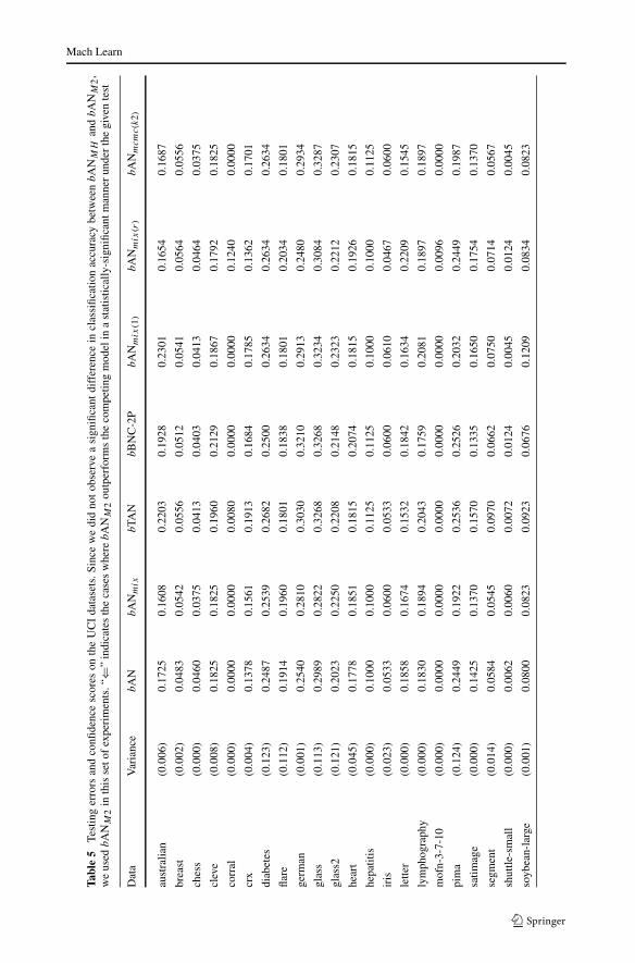
Mach Learn
Tabl
e5
Test
ing
erro
rsan
dco
nfide
nce
scor
eson
the
UC
Ida
tase
ts.S
ince
we
did
noto
bser
vea
sign
ifica
ntdi
ffer
ence
incl
assi
ficat
ion
accu
racy
betw
een
bAN
MH
and
bAN
M2,
we
used
bAN
M2
inth
isse
tof
expe
rim
ents
.“⇐
”in
dica
tes
the
case
sw
here
bAN
M2
outp
erfo
rms
the
com
petin
gm
odel
ina
stat
istic
ally
-sig
nific
antm
anne
run
der
the
give
nte
st
Dat
aV
aria
nce
bAN
bAN
mix
bTA
NbB
NC
-2P
bAN
mix
(1)
bAN
mix
(r)
bAN
mcm
c(k
2)
aust
ralia
n(0
.006
)0.
1725
0.16
080.
2203
0.19
280.
2301
0.16
540.
1687
brea
st(0
.002
)0.
0483
0.05
420.
0556
0.05
120.
0541
0.05
640.
0556
ches
s(0
.000
)0.
0460
0.03
750.
0413
0.04
030.
0413
0.04
640.
0375
clev
e(0
.008
)0.
1825
0.18
250.
1960
0.21
290.
1867
0.17
920.
1825
corr
al(0
.000
)0.
0000
0.00
000.
0080
0.00
000.
0000
0.12
400.
0000
crx
(0.0
04)
0.13
780.
1561
0.19
130.
1684
0.17
850.
1362
0.17
01
diab
etes
(0.1
23)
0.24
870.
2539
0.26
820.
2500
0.26
340.
2634
0.26
34
flare
(0.1
12)
0.19
140.
1960
0.18
010.
1838
0.18
010.
2034
0.18
01
germ
an(0
.001
)0.
2540
0.28
100.
3030
0.32
100.
2913
0.24
800.
2934
glas
s(0
.113
)0.
2989
0.28
220.
3268
0.32
680.
3234
0.30
840.
3287
glas
s2(0
.121
)0.
2023
0.22
500.
2208
0.21
480.
2323
0.22
120.
2307
hear
t(0
.045
)0.
1778
0.18
510.
1815
0.20
740.
1815
0.19
260.
1815
hepa
titis
(0.0
00)
0.10
000.
1000
0.11
250.
1125
0.10
000.
1000
0.11
25
iris
(0.0
23)
0.05
330.
0600
0.05
330.
0600
0.06
100.
0467
0.06
00
lette
r(0
.000
)0.
1858
0.16
740.
1532
0.18
420.
1634
0.22
090.
1545
lym
phog
raph
y(0
.000
)0.
1830
0.18
940.
2043
0.17
590.
2081
0.18
970.
1897
mof
n-3-
7-10
(0.0
00)
0.00
000.
0000
0.00
000.
0000
0.00
000.
0096
0.00
00
pim
a(0
.124
)0.
2449
0.19
220.
2536
0.25
260.
2032
0.24
490.
1987
satim
age
(0.0
00)
0.14
250.
1370
0.15
700.
1335
0.16
500.
1754
0.13
70
segm
ent
(0.0
14)
0.05
840.
0545
0.09
700.
0662
0.07
500.
0714
0.05
67
shut
tle-s
mal
l(0
.000
)0.
0062
0.00
600.
0072
0.01
240.
0045
0.01
240.
0045
soyb
ean-
larg
e(0
.001
)0.
0800
0.08
230.
0923
0.06
760.
1209
0.08
340.
0823
Mach Learn
Tabl
e5
(Con
tinu
ed)
Dat
aV
aria
nce
bAN
bAN
mix
bTA
NbB
NC
-2P
bAN
mix
(1)
bAN
mix
(r)
bAN
mcm
c(k
2)
vehi
cle
(0.0
43)
0.31
200.
3191
0.28
830.
3049
0.28
830.
3475
0.30
21
vote
(0.0
00)
0.05
060.
0529
0.09
200.
0713
0.07
800.
0529
0.05
29
wav
efor
m(0
.009
)0.
2121
0.20
890.
2532
0.20
430.
2323
0.20
870.
2187
Ave
rage
0.14
360.
1433
0.15
830.
1526
0.15
450.
1563
0.14
65
bTA
NbB
NC
-2P
bAN
mix
(1)
bAN
mix
(r)
bAN
mcm
c(k
2)
Wilc
oxon
SRte
stbA
N⇐
−3.7
13⇐
−2.7
18⇐
−3.4
84⇐
−3.6
06−0
.61
Frie
dman
/Bon
ferr
oni
bAN
⇐−3
.28
⇐−1
.66
⇐−2
.41
⇐−2
.34
−0.9
4
Mach Learn
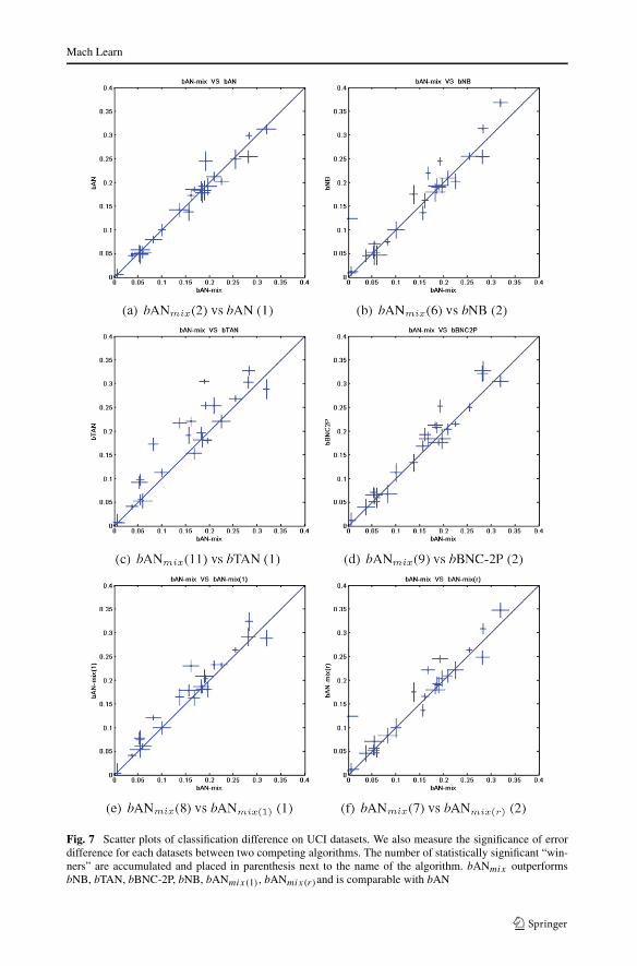
Fig. 7 Scatter plots of classification difference on UCI datasets. We also measure the significance of errordifference for each datasets between two competing algorithms. The number of statistically significant “win-ners” are accumulated and placed in parenthesis next to the name of the algorithm. bANmix outperformsbNB, bTAN, bBNC-2P, bNB, bANmix(1), bANmix(r)and is comparable with bAN

Mach Learn
Table 6 Classification error on the testing data. We divided the 25 datasets into three categories (each con-taining 7 to 9 sets) with respect to its classification variance (noise). For each category, the first row containsthe testing error, and the second row is the error difference between each competing algorithm and bAN (pos-itive differences correspond to lower error for bAN). bAN significantly outperforms bTAN and bBNC-2P indatasets with variance by having a sparser structure. Also, bAN is relatively resistant to noise, demonstratedby having comparable performance with bNB in datasets with mid or high variances
Datasets bAN bANmix bNB bTAN bBNC-2P bANmix(1) bANmix(r) bANmcmc(k2)
low 0.0767 0.0793 0.1032 0.0861 0.0811 0.0844 0.1034 0.0765
(σ 2 < 0.001) (+.0026) (+.0265) (+.0094) (+.0044) (+.0077) (+.0267) (−0.002)
mid 0.1586 0.1535 0.1582 0.1756 0.1688 0.1727 0.1578 0.1614
(0.001 ≤ σ 2 ≤ 0.1) (−.0051) (−.0004) (+.0170) (+.0102) (+.0141) (−.0008) (+.0028)
high 0.2299 0.2372 0.2417 0.2499 0.2456 0.2405 0.2483 0.2403
( σ 2 > 0.1) (+.0073) (+.0118) (+.0200) (+.0157) (+.0106) (+.0184) (+.0104)
the two basic strategies used in our formulation of boosted Bayesian network classi-fiers.
First, structures are beneficial in improving the performance of boosted Bayesian net-work classifiers. For example, bAN significantly outperformed bNB, especially in data-setswhere features are highly correlated with each other (such as Letter, etc). Also, bANmix sig-nificantly outperformed bANmix(r). We observed in the experiment that the edges randomlyselected by bANmix(r) often did not improve the classification accuracy on the training data.As a result, bANmix(r) usually terminated in the early stage of structure selection, with sim-ilar classification performance and model structures as bNB.
Second, since AdaBoost can overfit on noisy datasets, parsimonious structure selectionprovides the best compromise between modeling the structure of the data and controlling theclassifier capacity. For example, both bAN and bNB significantly outperform bBNC-2P andbTAN. This is also observed in the comparison between bANmix and bANmix(1). In noisydatasets like “Australian” and “crx”, bANmix(1), having a larger number of edges, performssignificantly worse than bANmix . Table 6 divides the datasets into three categories basedon the classification variance in the data. It is evident that bAN and bANmix significantlyoutperform bTAN and bBNC2P in the noisy datasets in Table 6.
Also, the combination of structure optimization with boosting bANmcmc(k2) does not out-performs bANmix . On the contrary, bANmix slightly outperforms bANmcmc(k2) on datasetswith larger variance, an indication that bANmix is more resistant to overfitting.
7 Comparison of computational cost
7.1 Computational complexity of bNB and bAN
Given a naive Bayes classifier with N attributes and training data with M samples, theML training complexity is O(NM), which is optimal when every attribute is observed andused for classification. Parameter boosting for a naive Bayes model is O(NMT ) where T
is the number of iterations of boosting. In our experiments, boosting seems to give goodperformance with a constant number (10–30) of iterations irrespective of the number ofattributes (ranging from 5 to 50). This is consistent with the finding of Elkan (1997).
bAN has a higher training complexity than bNB. Step 1 in the bAN algorithm has thecomputational complexity O(N2M), where N is the number of attributes and M is the
Mach Learn
amount of training data. Since we only add a maximum of N −1 edges to the network, steps2–4 have a worst case complexity O(NMT Smax), where Smax is the number of structuresanalyzed. Therefore bAN has O(N2M + NMT Smax) complexity. In our experiments, bANevaluates a very small number of additional structures as base structure.9 Therefore, bAN isvery efficient in practice.
bANmix on the other hand, has similar computational complexity as bAN. However, sincebANmix incrementally add new structures into the existing ensemble, bANmix does not eval-uate each new structure in all T steps as in bAN. Therefore, the computational complexityfor bANmix is O(N2M + NMT kSmax), where k < 1. We will show in the next section thatbANmix indeed requires less classifier evaluations than bAN.
7.2 Empirical analysis of computational cost
The variations in possible optimization schemes make a theoretical comparison of the train-ing cost for different Bayesian network classifiers challenging. Therefore we employ em-pirical training time in our analysis. All of the algorithms are implemented in C++ to sharecommon code bases. The experiments were conducted on a cluster of 3 GHz machines.
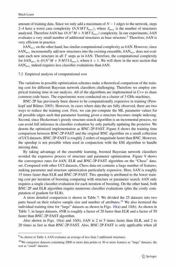
BNC-2P has previously been shown to be computationally expensive in training (Pern-kopf and Bilmes 2005). However, in cases where data the are fully observed, there are twoways to reduce the training cost. First, we can pre-compute the ML parameter values forall possible edges such that parameter learning given a structure becomes simple indexing.Second, since Heckerman’s greedy structure search algorithm is an incremental process, wecan avoid full inference in classifier evaluation by only partially updating the posterior. Wedenote the optimized implementation as BNC-2P-FAST. Figure 8 shows the training timecomparison between BNC-2P-FAST and the original BNC algorithm on a small collectionof UCI datasets. BNC-2P-FAST is roughly 2 orders of magnitude faster than BNC. However,the speedup is not possible when used in conjunction with the EM algorithm to handlemissing data.
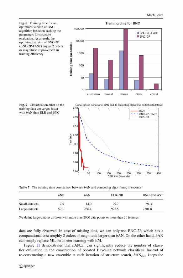
By taking advantage of the ensemble learning, boosted Bayesian network classifiersavoided the expensive process of structure and parameter optimization. Figure 9 showsthe convergence rates for bAN, ELR and BNC-2P-FAST algorithm on the “Chess” data-set. Compared with other UCI datasets, Chess data-set contains a large number of features,making parameter and structure optimization particularly expensive. Here, bAN is roughly15 times faster than ELR and BNC-2P-FAST. This speedup is attributed to the lower train-ing cost per iteration of boosting comparing with structure or parameter search. bAN onlyrequires a single classifier evaluation for each iteration of boosting. On the other hand, bothBNC-2P and ELR algorithm require numerous classifier evaluations (plus the costly com-putation of gradient for ELR).
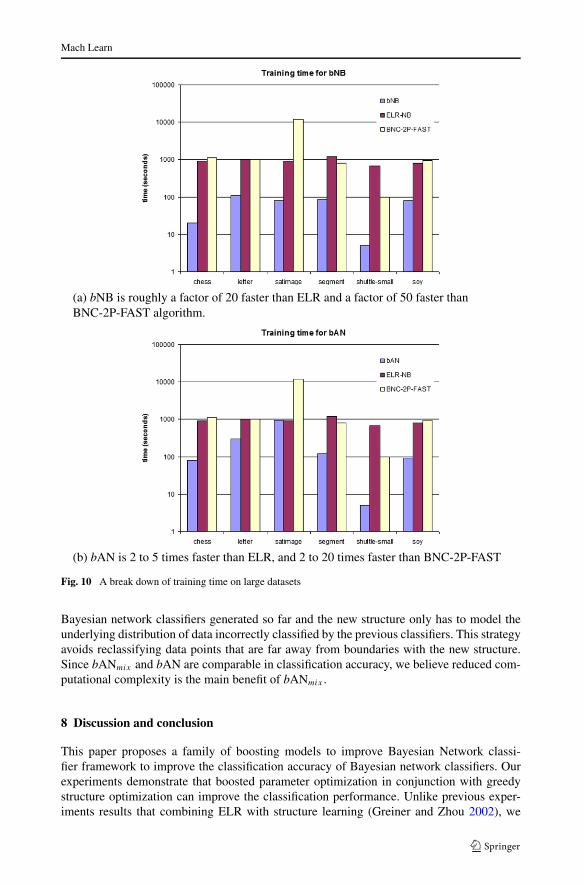
A more detailed comparison is shown in Table 7. We divided the 25 datasets into twoparts based on their relative sample size and number of attributes.10 We also itemized theindividual training time for “large” datasets as shown in Figs. 10(a) and 10(b). As shown inTable 7, in larger datasets, bNB is roughly a factor of 20 faster than ELR and a factor of 50faster than BNC-2P-FAST algorithm.
Also shown in Figs. 10(a) and 10(b), bAN is 2 to 5 times faster than ELR, and 2 to20 times as fast as than BNC-2P-FAST. Also, BNC-2P-FAST is only applicable when all
9As shown in Table 4, bAN evaluates an average of less than 2 additional structures.10We categorize datasets containing 2000 or more data points or 30 or more features as “large” datasets, therest as “small” datasets.
Mach Learn
Fig. 8 Training time for anoptimized version of BNCalgorithm based on caching theparameters for structureevaluation. As a result, theoptimized version of BNC-2P(BNC-2P-FAST) enjoys 2 ordersor magnitude improvement intraining efficiency
Fig. 9 Classification error on thetraining data converges fasterwith bAN than ELR and BNC
Table 7 The training time comparison between bAN and competing algorithms, in seconds
bNB bAN ELR-NB BNC-2P-FAST
Small-datasets 2.5 14.0 29.7 94.3
Large-datasets 59.1 266.4 925.5 2701.8
We define large-dataset as those with more than 2000 data points or more than 30 features
data are fully observed. In case of missing data, we can only use BNC-2P, which has acomputational cost roughly 2 orders of magnitude larger than bAN. On the other hand, bANcan simply replace ML parameter learning with EM.
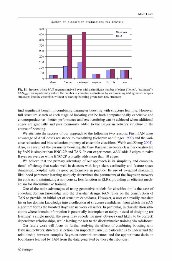
Figure 11 demonstrates that bANmix can significantly reduce the number of classi-fier evaluation in the construction of boosted Bayesian network classifiers. Instead ofre-constructing a new ensemble at each iteration of structure search, bANmix keeps the
Mach Learn
(a) bNB is roughly a factor of 20 faster than ELR and a factor of 50 faster thanBNC-2P-FAST algorithm.
(b) bAN is 2 to 5 times faster than ELR, and 2 to 20 times faster than BNC-2P-FAST
Fig. 10 A break down of training time on large datasets
Bayesian network classifiers generated so far and the new structure only has to model theunderlying distribution of data incorrectly classified by the previous classifiers. This strategyavoids reclassifying data points that are far away from boundaries with the new structure.Since bANmix and bAN are comparable in classification accuracy, we believe reduced com-putational complexity is the main benefit of bANmix .
8 Discussion and conclusion
This paper proposes a family of boosting models to improve Bayesian Network classi-fier framework to improve the classification accuracy of Bayesian network classifiers. Ourexperiments demonstrate that boosted parameter optimization in conjunction with greedystructure optimization can improve the classification performance. Unlike previous exper-iments results that combining ELR with structure learning (Greiner and Zhou 2002), we
Mach Learn
Fig. 11 In cases where bAN augments naive Bayes with a significant number of edges (“letter”, “satimage”),bANmix can significantly reduce the number of classifier evaluations by incrementing adding more complexstructures into the ensemble, without re-starting boosting given each new structure
find significant benefit in combining parameter boosting with structure learning. However,full structure search at each stage of boosting can be both computationally expensive andcounterproductive—better performance and less overfitting can be achieved when additionaledges are gradually and parsimoniously added to the Bayesian network structure in thecourse of boosting.
We attribute the success of our approach to the following two reasons. First, bAN takesadvantage of AdaBoost’s resistance to over-fitting (Schapire and Singer 1999) and the vari-ance reduction and bias reduction property of ensemble classifiers (Webb and Zheng 2004).Also, as a result of the parameter boosting, the base Bayesian network classifier constructedby bAN is simpler than BNC-2P and TAN. In our experiments, bAN adds 2 edges to naiveBayes on average while BNC-2P typically adds more than 10 edges.
We believe that the primary advantage of our approach is its simplicity and computa-tional efficiency that scales well in datasets with large class cardinality and feature spacedimension, coupled with its good performance in practice. Its use of weighted maximumlikelihood parameter learning uniquely determines the parameters of the Bayesian network(in contrast to minimizing a non-convex loss function in ELR), providing an efficient mech-anism for discriminative training.
One of the main advantages of using generative models for classification is the ease ofencoding domain knowledge into the classifier design. bAN relies on the construction ofTAN to provide an initial set of structure candidates. However, a user can readily translatehis or her domain knowledge into a collection of structure candidates, from which the bANalgorithm forms the boosted Bayesian network classifier. In particular, in classification situ-ations where domain information is potentially incomplete or noisy, instead of designing (orlearning) a single model, the users may encode the most obvious (and likely to be correct)dependence relationships, while leaving the rest to the discriminative training via AdaBoost.
Our future work will focus on further studying the effects of combining boosting withBayesian network structure selection. On important issue, in particular, is to understand therelationship between complex Bayesian network structures and the approximate decisionboundaries learned by bAN from the data generated by those distributions.
Mach Learn
Acknowledgements The authors would like to thank Matt Mullin for several fruitful discussions and forsuggesting the chain-structured model in Fig. 3. We would like to thank S. Charles Brubaker for his helpin constructing the factor graph in Fig. 12. We would also like to thank Pedro Domingos for his helpfulsuggestions on improving the speed and performance of the BNC-2P algorithm.
This material is based upon work which was supported in part by the National Science Foundation underNSF Grant IIS-0205507 and IIS-0413105.
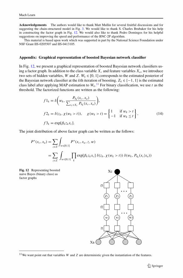
Appendix: Graphical representation of boosted Bayesian network classifier
In Fig. 12, we present a graphical representation of boosted Bayesian network classifiers us-ing a factor graph. In addition to the class variable Xc and feature variables Xa , we introducetwo sets of hidden variables, W and Z. Wk ∈ [0,1] corresponds to the estimated posterior ofthe Bayesian network classifier at the kth iteration of boosting. Zk ∈ {−1,1} is the estimatedclass label after applying MAP estimation to Wk .11 For binary classification, we use t as thethreshold. The factorized functions are written as the following:
f 1k = δ
(wk,
Pθk(xc, xa)∑
xc∈XcPθk
(xc, xa)
),
f 2k = δ(zk,χ(wk > t)), χ(wk > t) ={
1 if wk > t
−1 if wk ≤ t
}, (14)
f 3k = exp[βkzkxc].The joint distribution of above factor graph can be written as the follows:
P ∗(xc, xa) =∑
z∈Z
∫
w∈[0,1]P ∗(xc, xa, z,w)
=∑
z∈Z
∫
w∈[0,1]
∏
k
exp[βkzkxc] δ(zk,χ(wk > t)) δ(wk,Pθk(xc|xa))
Fig. 12 Representing boostednaive Bayes (binary class) asfactor graphs
11We want point out that variables W and Z are deterministic given the instantiation of the features.

Mach Learn
=∏
k
exp [βkψkxc], where ψk = χ(Pθk(xc|xa) > t)
where δ refers to Kronecker delta function.The ratio of the conditional distribution can then be expressed as:
P ∗(xc = 1|xa)
P ∗(xc = −1|xa)= P ∗(xc = 1, xa)
P ∗(xc = −1, xa)=
∏
k
exp[βkψk]exp[−βkψk] =
∏
k
exp[2βkψk]
=∏
k
exp
[ψk log
1 − errk
errk
]=
∏
k
(1 − errk
errk
)ψk
(15)
Equation 15 represents the posterior ratio of Discrete AdaBoost. We want to also point outthat given the values for ψ , Eq. 15 has similar functional form as naive Bayes under certainconstraints.12
References
Altun, Y., Tsochantaridis, I., & Hofmann, T. (2003). Hidden Markov support vector machines. In Proceedingsof the 20th international conference on machine learning (ICML) (pp. 3–10), Washington, DC.
Bauer, E., & Kohavi, R. (1999). An empirical comparison of voting classification algorithms: bagging, boost-ing, and variants. Machine Learning, 36(1–2), 105–139.
Blake, C. L., & Merz, C. J. (1998). UCI repository of machine learning databases. http://www.ics.uci.edu/~mlearn/MLRepository.html
Chelba, C., & Acero, A. (2004). Conditional maximum likelihood estimation of naive Bayes probability mod-els using rational function growth transform (Technical Report MSR-TR-2004-33). Microsoft.
Chickering, D. M., & Heckerman, D. (1997). Efficient approximations for the marginal likelihood of Bayesiannetworks with hidden variables. Machine Learning, 29(2–3), 181–212.
Choudhury, T., Rehg, J. M., Pavlovic, V., & Pentland, A. (2002). Boosting and structure learning in dynamicBayesian networks for audio-visual speaker detection. In Proceedings of the 16th international confer-ence on pattern recognition (vol. 3, pp. 789–794).
Chow, C. K., & Liu, C. N. (1968). Approximating discrete probability distributions with dependence trees.IEEE Transactions on Information Theory, 14(3), 462–467.
Cooper, G. F., & Herskovits, E. (1992). A Bayesian method for the induction of probabilistic networks fromdata. Machine Learning, 9, 309–347.
Cutting, D., Kupiec, J., Pedersen, J., & Sibun, P. (1992). A practical part-of-speech tagger. In Proceedings ofthe 3rd conference on applied natural language processing (pp. 133–140). Morristown: Association forComputational Linguistics.
Demsar, J. (2006). Statistical comparisons of classifiers over multiple data sets. Journal of Machine LearningResearch, 7, 1–30.
Devroye, L., Györfi, L., & Lugosi, G. (1996). A probabilistic theory of pattern recognition (p. 260).Dietterich, T. G. (2000). An experimental comparison of three methods for constructing ensembles of decision
trees: bagging, boosting, and randomization. Machine Learning, 40(2), 139–157.Dougherty, J., Kohavi, R., & Sahami, M. (1995). Supervised and unsupervised discretization of continuous
features. In Proceedings of the 12th international conference on machine learning (ICML) (pp. 194–202).
Drucker, H., & Cortes, C. (1996). Boosting decision trees. In Proceedings of the 8th advances in neuralinformation processing systems (NIPS) (pp. 470–485).
Duda, R. O., & Hart, P. E. (1973). Pattern classification and scene analysis. New York: Wiley-Interscience.
12When the positive error equals the negative error, and when xc is uniformly distributed,( 1−errk
errk
)ψk =( PDk
(ψk=xc)
PDk(ψk �=xc)
)ψk = PDk(ψk |xc=1)
PDk(ψk |xc=−1)
, which is analogous to the Maximum Likelihood parameters in sym-
metric naive Bayes. Instead of xa , ψ are the features for naive Bayes in this case.
Mach Learn
Elkan, C. (1997). Boosting and naive Bayesian learning (Technical Report CS97-557). Department of Com-puter Science and Engineering, University of California, San Diego.
Friedman, J. H. (1997). On bias, variance, 0/1-loss, and the curse-of-dimensionality. Data Mining and Knowl-edge Discovery, 1(1), 55–77.
Friedman, N., & Koller, D. (2000). Being Bayesian about network structure. In Proceedings of the 16thconference on uncertainty in artificial intelligence (UAI) (pp. 201–210), June 2000.
Friedman, N., Geiger, D., & Goldszmidt, M. (1997). Bayesian network classifiers. Machine Learning, 29,131–163.
Friedman, N., Getoor, L., Koller, D., & Pfeffer, A. (1999). Learning probabilistic relational models. In Pro-ceedings of the 16th international joint conference on artificial intelligence (IJCAI) (p. 1300–1309).
Friedman, J., Hastie, T., & Tibshirani, R. (2000). Additive logistic regression: a statistical view of boosting.The Annals of Statistics, 38(2), 337–374.
Greiner, R., & Zhou, W. (2002). Structural extension to logistic regression: discriminative parameter learningof belief net classifiers. In Proceedings of annual meeting of the American association for artificialintelligence (pp. 167–173).
Grossman, D., & Domingos, P. (2004). Learning Bayesian network classifiers by maximizing conditionallikelihood. In Proceedings of the 21st international conference on machine learning (ICML) (pp. 361–368). Banff: ACM Press.
Heckerman, D. (1995). A tutorial on learning with Bayesian networks (Technical Report MSR-TR-95-06).Microsoft Research.
Heckerman, D., Geiger, D., & Chickering, D. M. (1995). Learning Bayesian networks: the combination ofknowledge and statistical data. Machine Learning, 20(3), 197–243.
Jing, Y., Pavlovic, V., & Rehg, J. M. (2005). Efficient discriminative learning of Bayesian network classifiersvia boosted augmented naive Bayes. In Proceedings of the 22nd international conference on machinelearning (ICML) (pp. 369–376).
Jojic, V., Jojic, N., Meek, C., Geiger, D., Siepel, A., Haussler, D., & Heckerman, D. (2004). Efficient approx-imations for learning phylogenetic HMM models from data. Bioinformatics, 20(1), 161–168.
Keogh, E., & Pazzani, M. (1999). Learning augmented Bayesian classifiers: a comparison of distribution-based and classification-based approaches. In Proceedings of the 7th international workshop on artificialintelligence and statistics (pp. 225–230).
Kohavi, R., & John, G. H. (1997). Wrappers for feature subset selection. Artificial Intelligence, 97(1–2),273–324.
Kohavi, R., & Wolpert, D. H. (1996). Bias plus variance decomposition for zero-one loss functions. InL. Saitta (Ed.), Machine learning: proceedings of the thirteenth international conference (pp. 275–283).San Mateo: Morgan Kaufmann.
Lafferty, J., McCallum, A., & Pereira, F. (2001). Conditional random fields: probabilistic models for seg-menting and labeling sequence data. In Proceedings of the 18th international conference on machinelearning (ICML) (pp. 282–289).
Lam, W., & Bacchus, F. (1992). Learning Bayesian belief networks. an approach based on the mdl principle.Computational Intelligence, 10, 269–293.
Langley, P., Iba, W., & Thompson, K. (1992). An analysis of Bayesian classifiers. In Proceedings of the tenthnational conference on artificial intelligence (pp. 223–228). San Jose: AAAI Press.
McCallum, A., Freitag, D., & Pereira, F. (2000). Maximum entropy Markov models for information extractionand segmentation. In Proceedings of the 17th international conference on machine learning (ICML)(pp. 591–598), San Francisco, CA.
Nadas, A. (1983). A decision theoretic formulation of a training problem in speech recognition and a com-parison of training by unconditional versus conditional maximum likelihood. IEEE Transactions onAcoustics, Speech, & Signal Processing, 31(4), 814.
Ng, A. Y., & Jordan, M. I. (2002). On discriminative vs. generative classifiers: a comparison of logisticregression and naive Bayes. In Proceedings of the 14th conference on advances in neural informationprocessing systems (NIPS) (pp. 841–848).
Niculescu-Mizil, A., & Caruana, R. (2005). Obtaining calibrated probabilities from boosting. In Proceedingsof the 21st conference on uncertainty in artificial intelligence. Corvallis: AUAI Press.
Pavlovic, V., Garg, A., Rehg, J. M., & Huang, T. (2000). Multimodal speaker detection using error feedbackdynamic Bayesian networks. In 2000 IEEE computer society conference on computer vision and patternrecognition (CVPR) (Vol. 2, pp. 34–41).
Pavlovic, V., Garg, A., & Kasif, S. (2002). A Bayesian framework for combining gene predictions. Bioinfor-matics, 18(1), 19–27.
Pearl, J. (1988). Probabilistic reasoning in intelligent systems: networks of plausible inference. San Mateo:Morgan Kaufmann.
Mach Learn
Pernkopf, F., & Bilmes, J. (2005). Discriminative versus generative parameter and structure learning ofBayesian network classifiers. In Proceedings of the 22nd international conference on machine learn-ing (ICML) (pp. 657–664).
Rabiner, L., & Juang, B. H. (1993). Fundamentals of speech recognition. Englewood Cliffs: Prentice Hall.Rehg, J. M., Pavlovic, V., Huang, T. S., & Freeman, W. T. (2003). Special section on graphical models in
computer vision. IEEE Transactions on Pattern Analysis and Machine Intelligence, 25(7).Ridgeway, G., Madigan, D., Richardson, T., & O’Kane, J. (1998). Interpretable boosted naive Bayes classifi-
cation. In Proceedings of the 4th international conference on knowledge discovery and data mining.Schapire, R. E., & Singer, Y. (1999). Improved boosting using confidence-rated predictions. Machine Learn-
ing, 37(3), 297–336.Schapire, R. E., & Singer, Y. (2000). BoosTexter: a boosting-based system for text categorization. Machine
Learning, 39(2/3), 135–168.Schneiderman, H. (2004). Learning a restricted Bayesian network for object detection. In Proceedings of the
computer society conference on computer vision and pattern recognition (CVPR) (pp. 639–646), June2004.
Segal, E., Yelensky, R., & Koller, D. (2003). Genome-wide discovery of transcriptional modules from dnasequence and gene expression. Bioinformatics, 19(1), 273–282.
Taskar, B., Guestrin, C., & Koller, D. (2004). Max-margin Markov networks. In Proceedings of the 16thconference on advances in neural information processing systems (NIPS) (p. 102). Cambridge: MITPress.
Torralba, A., Murphy, K. P., & Freeman, W. T. (2004). Sharing features: efficient boosting procedures formulticlass object detection. In Proceedings of the IEEE conference on computer vision and patternrecognition (CVPR) (Vol. 2, pp. 762–769), Washington, DC, June 2004.
Webb, G., & Zheng, Z. (2004). Multistrategy ensemble learning: reducing error by combining ensemblelearning techniques. IEEE Transactions on Knowledge and Data Engineering, 16(8), 980–991.