Boom and Receptacle Autonomous Air Refueling Using …dnc.tamu.edu/projects/smartsensors/papers/archival/JGCDandAIAA... · Boom and Receptacle Autonomous Air Refueling Using a Visual

Boom and Receptacle Autonomous Air Refueling

Using a Visual Pressure Snake Optical Sensor

James Doebbler∗ and John Valasek†

Texas A&M University, College Station, TX 77843-3141

Mark J. Monda ‡ and Hanspeter Schaub §

Virginia Polytechnic Institute, Blacksburg, VA 24061-0203

Autonomous in-flight air refueling is an important capability for the future deploymentof unmanned air vehicles, since they will likely be ferried in flight to overseas theaters ofoperation instead of being shipped unassembled in containers. This paper introduces a visionsensor based on active deformable contour algorithms, and a relative navigation system thatenables precise and reliable boom and receptacle autonomous air refueling for non microsized unmanned air vehicles. The sensor is mounted on the tanker aircraft near the boom,and images a single passive target image painted near the refueling receptacle on the receiveraircraft. Controllers are developed for the automatic control of the refueling boom, and for thestation keeping controller of the receiver aircraft. The boom controller is integrated with theactive deformable contour sensor system, and feasibility of the total system is demonstrated bysimulated docking maneuvers in the presence of various levels of turbulence. Results indicatethat the integrated sensor and controller enables precise boom and receptacle air refueling,including consideration of realistic measurement errors and disturbances.

I. Introduction

There are currently two approaches used for air refueling. The probe-and-drogue refu-eling system is the standard for the United States Navy and the air forces of most othernations. In this method, the tanker trails a hose with a flexible “basket”, called a drogue,at the end. The drogue is aerodynamically stabilized. It is the responsibility of the pilotof the receiver aircraft to maneuver the receiver’s probe into the drogue. This methodis used for small, agile aircraft such as fighters because both the hose and drogue areflexible and essentially passive during re-fueling; a human operator is not required on thetanker.1–3 Autonomous in-flight refueling using a probe-and-drogue system is basicallya docking situation that probably requires 2 cm accuracy in the relative position of therefueling probe (from the receiving aircraft) with respect to the drogue (from the tanker)during the end-game. This specification is based on the geometry of the existing probe anddrogue hardware, and the need to ensure that the tip of the probe contacts only the innersleeve of the receptacle and not the more lightly constructed and easily damaged shroud.4

The United States Air Force uses the flying boom developed by Boeing. The boomapproach is supervised and controlled by a human operator from a station near the rearof the tanker aircraft, who is responsible for “flying” the boom into the refueling port onthe receiver aircraft. In this method, the job of the receiver aircraft is to maintain properrefueling position with respect to the tanker, and leave the precision control function tothe human operator in the tanker.2

∗Graduate Research Assistant, Flight Simulation Laboratory, Aerospace Engineering Department. Student Member [email protected]

†Associate Professor and Director, Flight Simulation Laboratory, Aerospace Engineering Department. Associate FellowAIAA. [email protected]

‡Graduate Research Assistant, Aerospace and Ocean Engineering Department. Student Member AIAA. [email protected]§Assistant Professor, Aerospace and Ocean Engineering Department. Member AIAA. [email protected]

1 of 23

American Institute of Aeronautics and Astronautics

AIAA Atmospheric Flight Mechanics Conference and Exhibit21 - 24 August 2006, Keystone, Colorado

AIAA 2006-6504

Copyright © 2006 by John Valasek, JamesDoebbler, Mark J. Monda, and Hanspeter Schaub. Published by the American Institute of Aeronautics and Astronautics, Inc., with permission.

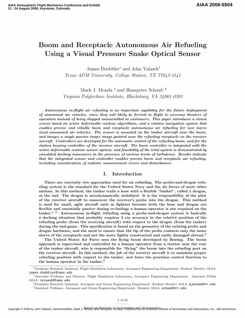
Figure 1. B-1B Lancer Refueling From a KC-10 Extender Using the Boom and Receptacle Method

Regardless of the type of autonomous refueling to be conducted, the maturation of thetechnology requires several issues to be addressed, the most fundamental being the lackof sufficiently accurate/reliable relative motion sensors.5 Some methods that have beenconsidered for determining relative position in a refueling scenario include measurementsderived from the Global Positioning System (GPS), measurements derived from both pas-sive and active machine vision, and visual servoing with pattern recognition software.6–10

GPS measurements have been made with 1 cm to 2 cm accuracy for formation flying, butproblems associated with lock-on, integer ambiguity, low bandwidth, and distortions dueto wake effects from the tanker present challenges for application to in-flight refueling.Pattern recognition codes are not sufficiently reliable in all lighting conditions, and withadequate fault tolerance, may require large amounts of computational power in order toconverge with sufficient confidence to a solution.6–8

Machine vision based techniques use optical markers to determine relative orientationand position of the tanker and the UAV. The drawback of the machine vision based tech-niques is the assumption that all the optical markers are always visible and functional.Reference11 proposes an alternative approach where the pose estimation does not dependon optical markers but on Feature Extraction methods, using specific corner detection al-gorithms. Special emphasis was placed on evaluating the accuracy, required computationaleffort, and robustness to different sources of noise. Closed loop simulations were performedusing a detailed Simulink-based simulation environment to reproduce boom and receptacledocking maneuvers.

Another approach is an active vision based navigation system called VisNav. VisNavprovides a high precision six degree-of-freedom information for real-time navigation appli-cations.12–14 VisNav is a cooperative vision technology in which a set of beacons mountedon a target body (e.g., the receiver aircraft) are supervised by a VisNav sensor mountedon a second body (e.g., the boom). VisNav structures the light in the frequency domain,analogous to radar, so that discrimination and target identification are near-trivial even in anoisy ambient environment. Controllers which use the VisNav sensor have been developedand evaluated specifically for probe and drogue autonomous air refueling.15–22In principle,the VisNav system could work with legacy boom and receptacle refueling systems since theonly major equipment changes are mounting the VisNav sensor to the boom and attachingfour or more Light Emitting Diode (LED) beacon lights to the forebody of the receiveraircraft, or vice versa.

Another class of sensing methods are the active deformable contour algorithms. Thesemethods segment the target area of the image by having a closed, non-intersecting contour

2 of 23


iterate across the image and track a target. In 1987 Kass et al. proposed the original activedeformable model to track targets within an images stream.23 They are also known as visualsnakes. For application to the end game docking problem of autonomous air refueling, avisual snake optical sensor mounted on the boom would acquire and track a geometricpattern painted on the receiver aircraft, and develop a relative navigation solution which isthen passed to a boom control system. This approach does not use pattern recognition, ispassive, and highly robust in various lighting conditions. Although it does not provide sixdegree-of-freedom data, this is not a penalty for boom and receptacle autonomous refuelingsince the boom requires only two rotations and one translation to successfully engage thereceptacle.

Figure 2. Conceptual Picture of a KC-135 Refueling a Predator UAV

Referring to Fig. 2, the system proposed in this paper is comprised of a receiver aircraft(in this case an Unmanned Air Vehicle (UAV)) equipped with a GPS sensor, and an onboardflight controller which permits it to station keep in a 3D box of specified dimensions,relative to the tanker aircraft. The receiver aircraft has a visual docking target paintedon its forebody, similar to the target painted on the forebody of the B-1B in Fig. 1. Thetanker aircraft is equipped with two sensors dedicated to autonomous air refueling. Thefirst sensor accurately measures the angular position of the boom at the pivot point, as wellas the length of the boom, thereby providing a measurement of the tip of the boom. Thesecond sensor is the visual pressure snake sensor, which is mounted on the rear of the tankerand oriented so that it possesses a clear, unobstructed field-of-view of the visual dockingtarget painted on the receiver aircraft’s forebody. For night refueling operations, the visualtarget painted on the receiver aircraft is illuminated by a light installed on the tanker.An automatic control system for the refueling boom receives estimates of the refuelingreceptacle position from the visual pressure snakes sensor, and steers the boom tip into it.There are no controller commands which would require a high speed, high bandwidth datalink being passed between the tanker and receiver aircraft. A communication link handlesinitiation and termination of the refueling sequence.

This paper develops a vision based relative navigation system that uses a visual pres-sure snakes optical sensor integrated with an automatic boom controller for autonomousboom and receptacle air refueling. The capability of this system to accurately estimate

3 of 23


the position of the receptacle, and then automatically steer the boom into it in light andmoderate atmospheric turbulence conditions, is demonstrated using non real-time simula-tion. Detailed software models of the optical sensor system are integrated with the boomand station keeping controllers, and evaluated with refueling maneuvers on a six degree-of-freedom simulation. Test cases consisting of initial positioning offsets in still air, andmaneuvers in turbulence, are used to evaluate the combined performance of the opticalsensor, boom controller, and station keeping controller system. For the refueling scenarioinvestigated here, only the end-game docking maneuver is considered. It is assumed thatthe tanker and receiver have already rendezvoused, and that the tanker is flying straightahead at constant speed. The receiver aircraft is positioned aft of the tanker in trimmedflight, and an onboard flight controller maintains position within a 3D box relative the tothe tanker.

The paper is organized as follows. First the basic working principles and componentsof the visual pressure snakes navigation sensor is presented in Section II, detailing thealgorithm and navigation solution, performance, forced perspective target setup, and errorsensitivities. This is followed by a description of the boom model in Section III, andderivation of the Proportional-Integral-Filter optimal Nonzero Setpoint controller(PIF-NZSP) boom control law in Section IV. The receiver aircraft station keeping controlleris developed in Section V, and the tanker and receiver aircraft linear state-space modelsare developed in Section VI. In Section VII, test cases using the Dryden gust modelwith light and moderate turbulence is used to assess system performance and disturbanceaccommodation characteristics in the presence of exogenous inputs. Finally, conclusionsand recommendations for further work are presented in Section VIII.

II. Visual Pressure Snakes Navigation Sensor

A. Visual Relative Motion Sensing

A critical technology for autonomous air refueling is a sensor for measuring the relativeposition and orientation between the receiver aircraft and the tanker aircraft. Becauserapid control corrections are required for docking, especially in turbulence, the navigationsensor must provide accurate, high-frequency updates. The proposed autonomous refuelingmethod uses color statistical pressure snakes24–26 to sense the relative position of the targetaircraft with respect to the tanker craft. Statistical pressure snakes methods, or visualsnakes, segment the target area of the image and track the target with a closed, non-intersecting contour. Hardware experiments verify that visual snakes can provide relativeposition measurements at rates of 30 Hz even using a standard, off-the-shelf 800 MHzprocessor.27 The visual snake provides not only information about the target size andcentroid location, but also provides some information about the target shape through theprincipal axes lengths. The proposed relative motion sensor employs a simple, rear-facingcamera mounted on the tanker aircraft, while the receiving vehicle has a visual targetpainted on its forebody near the refueling receptacle. Because the nominal relative positionbetween the aircraft during a refueling maneuver is fixed, the relative heading and rangeto the receiver aircraft is accurately determined from the target image center of mass andprincipal axes sizes.

B. Visual Snake Algorithm

In 1987 Kass et al. proposed the original active deformable model to track targets withinan images stream.28 Also referred to as a visual snake, the parametric curve is of the form

S(u) = I(x(u), y(u))′, u = [0, 1] (1)

where I is the stored image. This curve is placed into an image-gradient-derived potentialfield and allowed to change its shape and position in order to minimize the energy E alongthe length of the curve S(u). The energy function is expressed as:28

E =

∫ 1

0

[Eint(S(u)) +Eimg(S(u), I)

]du (2)

where Eint is the internal energy defined as

Eint =α

2

∣∣∣∣ ∂∂uS(u)

∣∣∣∣2 +β

2

∣∣∣∣ ∂2

∂u2S(u)

∣∣∣∣2 du (3)

4 of 23


Hue

Valu

e

Saturation

0

10

1

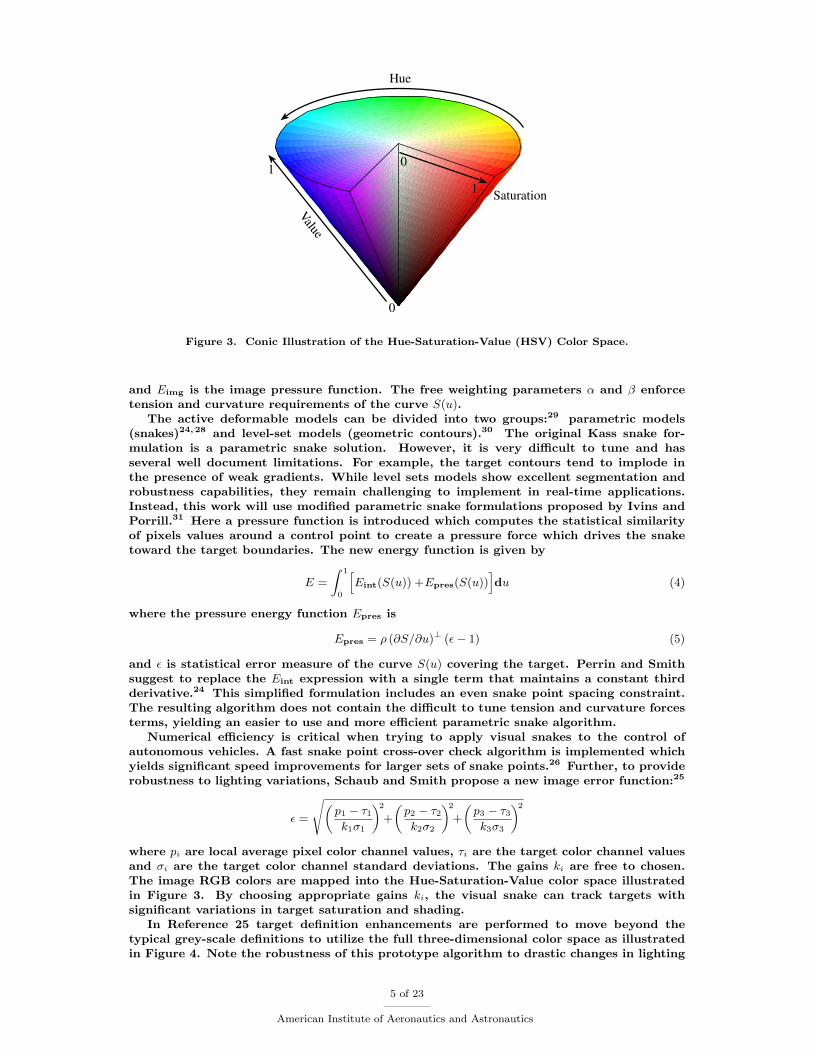
Figure 3. Conic Illustration of the Hue-Saturation-Value (HSV) Color Space.

and Eimg is the image pressure function. The free weighting parameters α and β enforcetension and curvature requirements of the curve S(u).

The active deformable models can be divided into two groups:29 parametric models(snakes)24,28 and level-set models (geometric contours).30 The original Kass snake for-mulation is a parametric snake solution. However, it is very difficult to tune and hasseveral well document limitations. For example, the target contours tend to implode inthe presence of weak gradients. While level sets models show excellent segmentation androbustness capabilities, they remain challenging to implement in real-time applications.Instead, this work will use modified parametric snake formulations proposed by Ivins andPorrill.31 Here a pressure function is introduced which computes the statistical similarityof pixels values around a control point to create a pressure force which drives the snaketoward the target boundaries. The new energy function is given by

E =

∫ 1

0

[Eint(S(u)) +Epres(S(u))

]du (4)

where the pressure energy function Epres is

Epres = ρ (∂S/∂u)⊥ (ε− 1) (5)

and ε is statistical error measure of the curve S(u) covering the target. Perrin and Smithsuggest to replace the Eint expression with a single term that maintains a constant thirdderivative.24 This simplified formulation includes an even snake point spacing constraint.The resulting algorithm does not contain the difficult to tune tension and curvature forcesterms, yielding an easier to use and more efficient parametric snake algorithm.

Numerical efficiency is critical when trying to apply visual snakes to the control ofautonomous vehicles. A fast snake point cross-over check algorithm is implemented whichyields significant speed improvements for larger sets of snake points.26 Further, to providerobustness to lighting variations, Schaub and Smith propose a new image error function:25

ε =

√(p1 − τ1k1σ1

)2

+

(p2 − τ2k2σ2

)2

+

(p3 − τ3k3σ3

)2

where pi are local average pixel color channel values, τi are the target color channel valuesand σi are the target color channel standard deviations. The gains ki are free to chosen.The image RGB colors are mapped into the Hue-Saturation-Value color space illustratedin Figure 3. By choosing appropriate gains ki, the visual snake can track targets withsignificant variations in target saturation and shading.

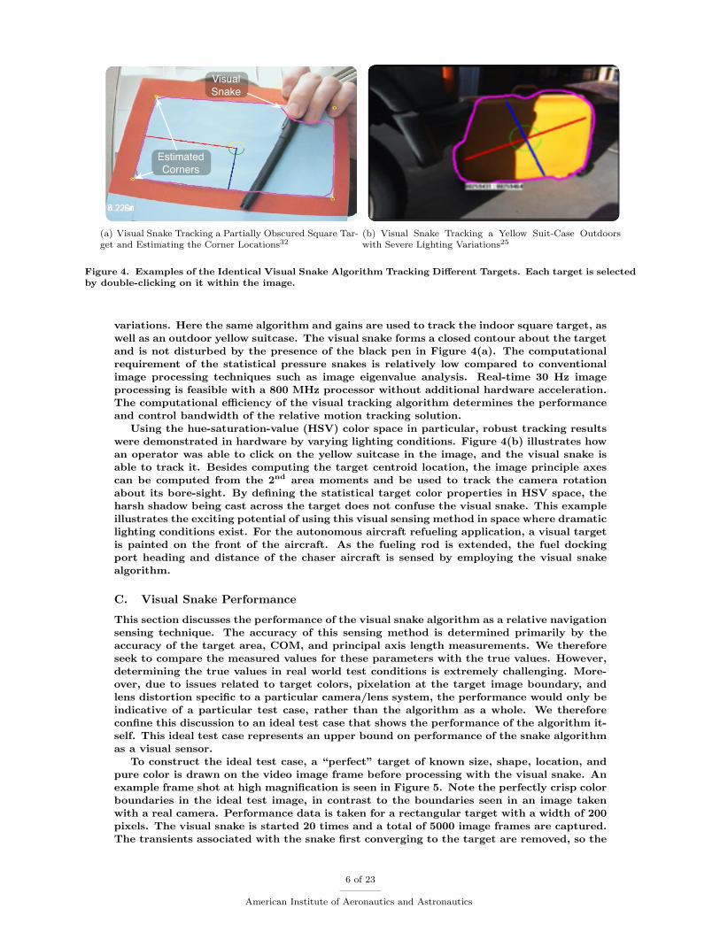
In Reference 25 target definition enhancements are performed to move beyond thetypical grey-scale definitions to utilize the full three-dimensional color space as illustratedin Figure 4. Note the robustness of this prototype algorithm to drastic changes in lighting

5 of 23


Visual Snake

EstimatedCorners

(a) Visual Snake Tracking a Partially Obscured Square Tar-get and Estimating the Corner Locations32

(b) Visual Snake Tracking a Yellow Suit-Case Outdoorswith Severe Lighting Variations25

Figure 4. Examples of the Identical Visual Snake Algorithm Tracking Different Targets. Each target is selectedby double-clicking on it within the image.

variations. Here the same algorithm and gains are used to track the indoor square target, aswell as an outdoor yellow suitcase. The visual snake forms a closed contour about the targetand is not disturbed by the presence of the black pen in Figure 4(a). The computationalrequirement of the statistical pressure snakes is relatively low compared to conventionalimage processing techniques such as image eigenvalue analysis. Real-time 30 Hz imageprocessing is feasible with a 800 MHz processor without additional hardware acceleration.The computational efficiency of the visual tracking algorithm determines the performanceand control bandwidth of the relative motion tracking solution.

Using the hue-saturation-value (HSV) color space in particular, robust tracking resultswere demonstrated in hardware by varying lighting conditions. Figure 4(b) illustrates howan operator was able to click on the yellow suitcase in the image, and the visual snake isable to track it. Besides computing the target centroid location, the image principle axescan be computed from the 2nd area moments and be used to track the camera rotationabout its bore-sight. By defining the statistical target color properties in HSV space, theharsh shadow being cast across the target does not confuse the visual snake. This exampleillustrates the exciting potential of using this visual sensing method in space where dramaticlighting conditions exist. For the autonomous aircraft refueling application, a visual targetis painted on the front of the aircraft. As the fueling rod is extended, the fuel dockingport heading and distance of the chaser aircraft is sensed by employing the visual snakealgorithm.

C. Visual Snake Performance

This section discusses the performance of the visual snake algorithm as a relative navigationsensing technique. The accuracy of this sensing method is determined primarily by theaccuracy of the target area, COM, and principal axis length measurements. We thereforeseek to compare the measured values for these parameters with the true values. However,determining the true values in real world test conditions is extremely challenging. More-over, due to issues related to target colors, pixelation at the target image boundary, andlens distortion specific to a particular camera/lens system, the performance would only beindicative of a particular test case, rather than the algorithm as a whole. We thereforeconfine this discussion to an ideal test case that shows the performance of the algorithm it-self. This ideal test case represents an upper bound on performance of the snake algorithmas a visual sensor.

To construct the ideal test case, a “perfect” target of known size, shape, location, andpure color is drawn on the video image frame before processing with the visual snake. Anexample frame shot at high magnification is seen in Figure 5. Note the perfectly crisp colorboundaries in the ideal test image, in contrast to the boundaries seen in an image takenwith a real camera. Performance data is taken for a rectangular target with a width of 200pixels. The visual snake is started 20 times and a total of 5000 image frames are captured.The transients associated with the snake first converging to the target are removed, so the

6 of 23


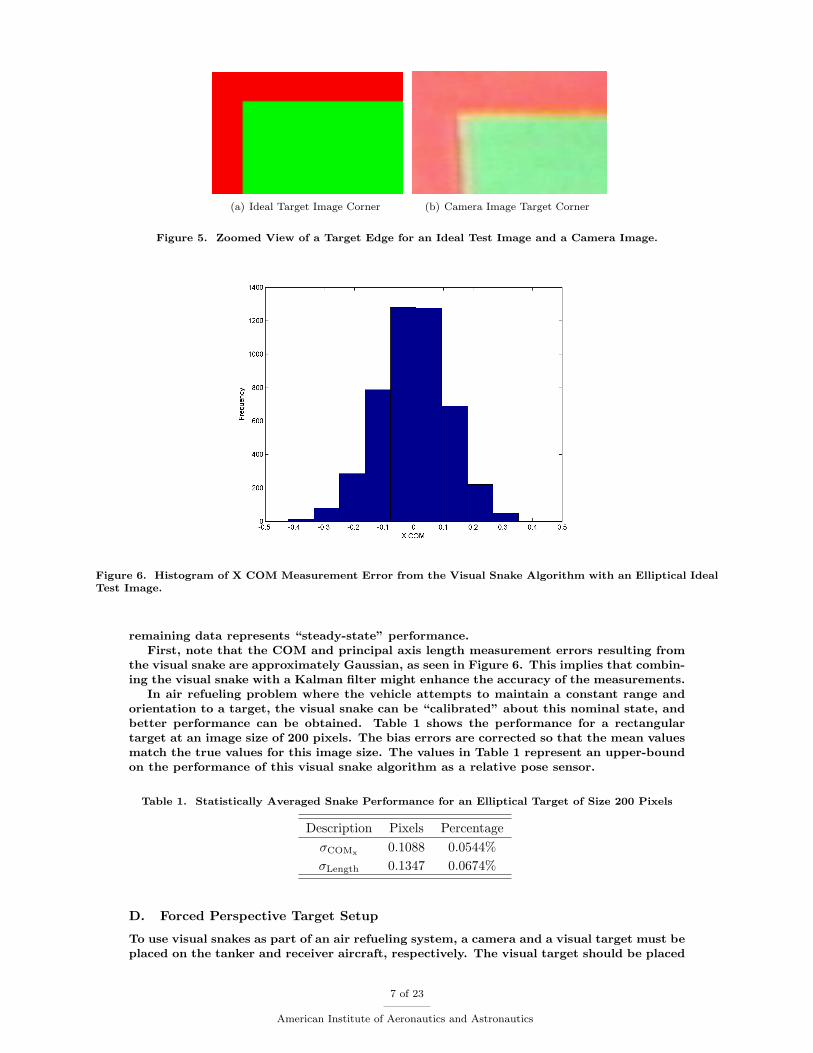
(a) Ideal Target Image Corner (b) Camera Image Target Corner

Figure 5. Zoomed View of a Target Edge for an Ideal Test Image and a Camera Image.

Figure 6. Histogram of X COM Measurement Error from the Visual Snake Algorithm with an Elliptical IdealTest Image.

remaining data represents “steady-state” performance.First, note that the COM and principal axis length measurement errors resulting from

the visual snake are approximately Gaussian, as seen in Figure 6. This implies that combin-ing the visual snake with a Kalman filter might enhance the accuracy of the measurements.

In air refueling problem where the vehicle attempts to maintain a constant range andorientation to a target, the visual snake can be “calibrated” about this nominal state, andbetter performance can be obtained. Table 1 shows the performance for a rectangulartarget at an image size of 200 pixels. The bias errors are corrected so that the mean valuesmatch the true values for this image size. The values in Table 1 represent an upper-boundon the performance of this visual snake algorithm as a relative pose sensor.

Table 1. Statistically Averaged Snake Performance for an Elliptical Target of Size 200 Pixels

Description Pixels PercentageσCOMx 0.1088 0.0544%σLength 0.1347 0.0674%

D. Forced Perspective Target Setup

To use visual snakes as part of an air refueling system, a camera and a visual target must beplaced on the tanker and receiver aircraft, respectively. The visual target should be placed

7 of 23


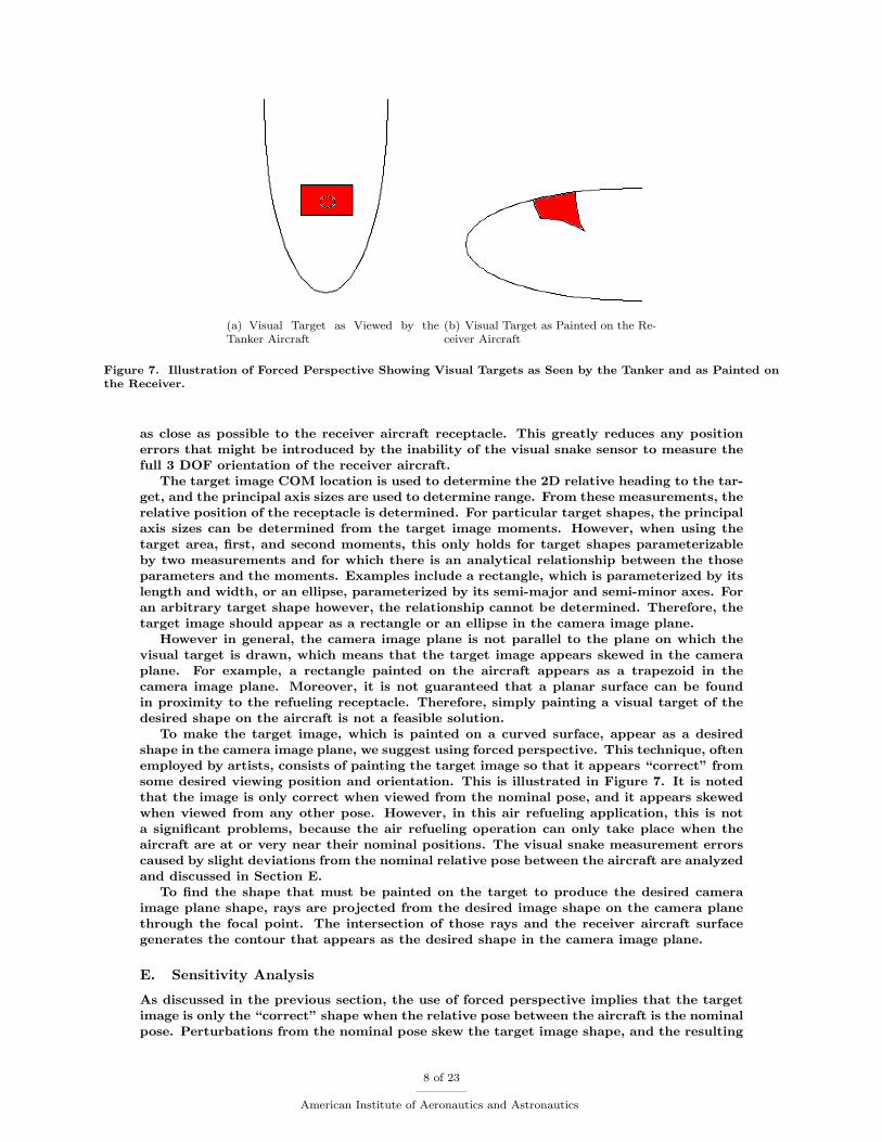
(a) Visual Target as Viewed by theTanker Aircraft

(b) Visual Target as Painted on the Re-ceiver Aircraft

Figure 7. Illustration of Forced Perspective Showing Visual Targets as Seen by the Tanker and as Painted onthe Receiver.

as close as possible to the receiver aircraft receptacle. This greatly reduces any positionerrors that might be introduced by the inability of the visual snake sensor to measure thefull 3 DOF orientation of the receiver aircraft.

The target image COM location is used to determine the 2D relative heading to the tar-get, and the principal axis sizes are used to determine range. From these measurements, therelative position of the receptacle is determined. For particular target shapes, the principalaxis sizes can be determined from the target image moments. However, when using thetarget area, first, and second moments, this only holds for target shapes parameterizableby two measurements and for which there is an analytical relationship between the thoseparameters and the moments. Examples include a rectangle, which is parameterized by itslength and width, or an ellipse, parameterized by its semi-major and semi-minor axes. Foran arbitrary target shape however, the relationship cannot be determined. Therefore, thetarget image should appear as a rectangle or an ellipse in the camera image plane.

However in general, the camera image plane is not parallel to the plane on which thevisual target is drawn, which means that the target image appears skewed in the cameraplane. For example, a rectangle painted on the aircraft appears as a trapezoid in thecamera image plane. Moreover, it is not guaranteed that a planar surface can be foundin proximity to the refueling receptacle. Therefore, simply painting a visual target of thedesired shape on the aircraft is not a feasible solution.

To make the target image, which is painted on a curved surface, appear as a desiredshape in the camera image plane, we suggest using forced perspective. This technique, oftenemployed by artists, consists of painting the target image so that it appears “correct” fromsome desired viewing position and orientation. This is illustrated in Figure 7. It is notedthat the image is only correct when viewed from the nominal pose, and it appears skewedwhen viewed from any other pose. However, in this air refueling application, this is nota significant problems, because the air refueling operation can only take place when theaircraft are at or very near their nominal positions. The visual snake measurement errorscaused by slight deviations from the nominal relative pose between the aircraft are analyzedand discussed in Section E.

To find the shape that must be painted on the target to produce the desired cameraimage plane shape, rays are projected from the desired image shape on the camera planethrough the focal point. The intersection of those rays and the receiver aircraft surfacegenerates the contour that appears as the desired shape in the camera image plane.

E. Sensitivity Analysis

As discussed in the previous section, the use of forced perspective implies that the targetimage is only the “correct” shape when the relative pose between the aircraft is the nominalpose. Perturbations from the nominal pose skew the target image shape, and the resulting

8 of 23


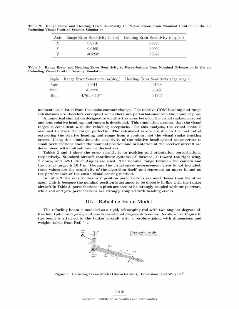
Table 2. Range Error and Heading Error Sensitivity to Perturbations from Nominal Position in the airRefueling Visual Position Sensing Simulation

Axis Range Error Sensitivity (m/m) Heading Error Sensitivity (deg./m)X 0.8756 0.0569Y 0.0169 0.0009Z -0.5232 0.0372

Table 3. Range Error and Heading Error Sensitivity to Perturbations from Nominal Orientation in the airRefueling Visual Position Sensing Simulation

Angle Range Error Sensitivity (m/deg.) Heading Error Sensitivity (deg./deg.)Yaw 0.0011 0.1606Pitch -0.1228 0.0460Roll 4.761× 10−4 0.1405

moments calculated from the snake contour change. The relative COM heading and rangecalculations are therefore corrupted when there are perturbations from the nominal pose.

A numerical simulation designed to identify the error between the visual snake-measuredand true relative headings and ranges is developed. This simulation assumes that the visualtarget is coincident with the refueling receptacle. For this analysis, the visual snake isassumed to track the target perfectly. The calculated errors are due to the method ofextracting the relative heading and range from a contour, not the visual snake trackingerrors. Using this simulation, the sensitivity of the relative heading and range errors tosmall perturbations about the nominal position and orientation of the receiver aircraft aredetermined with finite-difference derivatives.

Tables 2 and 3 show the error sensitivity to position and orientation perturbations,respectively. Standard aircraft coordinate systems (X forward, Y toward the right wing,Z down) and 3-2-1 Euler Angles are used. The nominal range between the camera andthe visual target is 10.7 m. Because the visual snake measurement error is not included,these values are the sensitivity of the algorithm itself, and represent an upper bound onthe performance of the entire visual sensing method.

In Table 2, the sensitivities to Y position perturbations are much lower than the otheraxes. This is because the nominal position is assumed to be directly in line with the tankeraircraft.In Table 3, perturbations in pitch are seen to be strongly coupled with range errors,while roll and yaw perturbations are strongly coupled with heading errors.

III. Refueling Boom Model

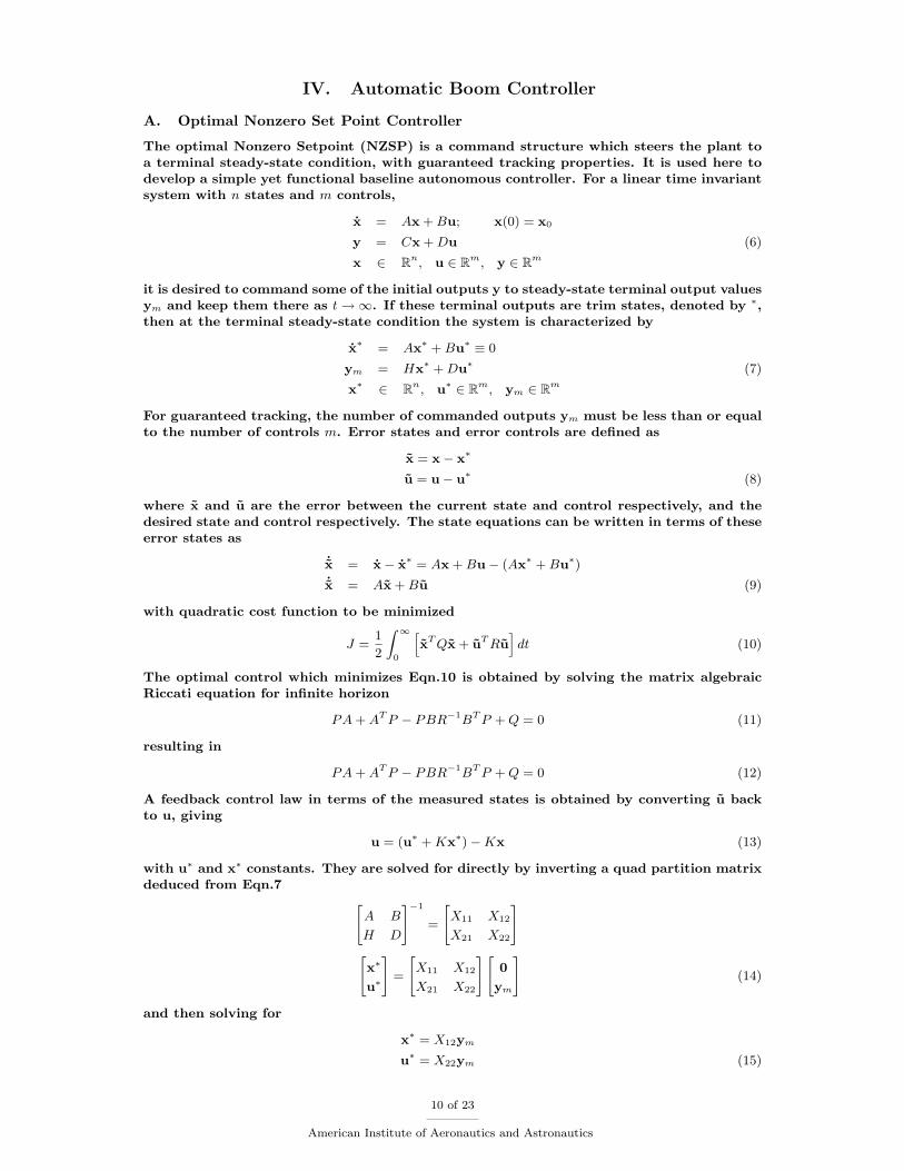
The refueling boom is modeled as a rigid, telescoping rod with two angular degrees-of-freedom (pitch and yaw), and one translational degree-of-freedom. As shown in Figure 8,the boom is attached to the tanker aircraft with a resolute joint, with dimensions andweights taken from Ref.11 c

Figure 8. Refueling Boom Model Characteristics, Dimensions, and Weights11

9 of 23


IV. Automatic Boom Controller

A. Optimal Nonzero Set Point Controller

The optimal Nonzero Setpoint (NZSP) is a command structure which steers the plant toa terminal steady-state condition, with guaranteed tracking properties. It is used here todevelop a simple yet functional baseline autonomous controller. For a linear time invariantsystem with n states and m controls,

x = Ax +Bu; x(0) = x0

y = Cx +Du (6)

x ∈ Rn, u ∈ Rm, y ∈ Rm

it is desired to command some of the initial outputs y to steady-state terminal output valuesym and keep them there as t→∞. If these terminal outputs are trim states, denoted by ∗,then at the terminal steady-state condition the system is characterized by

x∗ = Ax∗ +Bu∗ ≡ 0

ym = Hx∗ +Du∗ (7)

x∗ ∈ Rn, u∗ ∈ Rm, ym ∈ Rm

For guaranteed tracking, the number of commanded outputs ym must be less than or equalto the number of controls m. Error states and error controls are defined as

x = x− x∗

u = u− u∗ (8)

where x and u are the error between the current state and control respectively, and thedesired state and control respectively. The state equations can be written in terms of theseerror states as

˙x = x− x∗ = Ax +Bu− (Ax∗ +Bu∗)

˙x = Ax +Bu (9)

with quadratic cost function to be minimized

J =1

2

∫ ∞

0

[xTQx + uTRu

]dt (10)

The optimal control which minimizes Eqn.10 is obtained by solving the matrix algebraicRiccati equation for infinite horizon

PA+ATP − PBR−1BTP +Q = 0 (11)

resulting in


A feedback control law in terms of the measured states is obtained by converting u backto u, giving

u = (u∗ +Kx∗)−Kx (13)

with u∗ and x∗ constants. They are solved for directly by inverting a quad partition matrixdeduced from Eqn.7 [

A B

H D

]−1

=

[X11 X12

X21 X22

][x∗

u∗

]=

[X11 X12

X21 X22

] [0

ym

](14)

and then solving for

x∗ = X12ym

u∗ = X22ym (15)

10 of 23


Upon substitution in Eqn.13 the control law implementation equation becomes

u = (X22 +KX12)ym −Kx (16)

For the optimal control policy u to be admissible, the quad partition matrix must beinvertible. Therefore, the equations for x∗ and u∗ must be linearly independent, and thenumber of outputs or states that can be driven to a constant value must be less than orequal to the number of available controls. An advantage of this controller is the guaranteeof perfect tracking of a number of outputs equal to the number of controls, independentof the value of the gains, provided they are stabilizing. The gains can be designed usingany desired technique, and only affect the transient performance, and not the guarantee ofsteady-state performance.

B. Proportional-Integral-Filter Nonzero Setpoint Controller

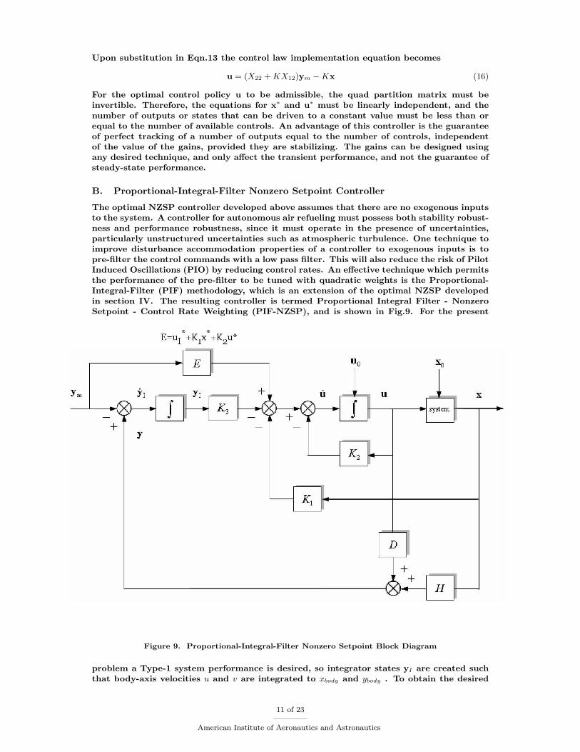
The optimal NZSP controller developed above assumes that there are no exogenous inputsto the system. A controller for autonomous air refueling must possess both stability robust-ness and performance robustness, since it must operate in the presence of uncertainties,particularly unstructured uncertainties such as atmospheric turbulence. One technique toimprove disturbance accommodation properties of a controller to exogenous inputs is topre-filter the control commands with a low pass filter. This will also reduce the risk of PilotInduced Oscillations (PIO) by reducing control rates. An effective technique which permitsthe performance of the pre-filter to be tuned with quadratic weights is the Proportional-Integral-Filter (PIF) methodology, which is an extension of the optimal NZSP developedin section IV. The resulting controller is termed Proportional Integral Filter - NonzeroSetpoint - Control Rate Weighting (PIF-NZSP), and is shown in Fig.9. For the present

Figure 9. Proportional-Integral-Filter Nonzero Setpoint Block Diagram

problem a Type-1 system performance is desired, so integrator states yI are created suchthat body-axis velocities u and v are integrated to xbody and ybody . To obtain the desired

11 of 23


filtering of the controls, the rates of the controls are also added as states u1. The optimalNZSP is extended into the optimal PIF-NZSP structure by first creating the integral ofthe commanded error

yI = y − ym; yI ∈ Rm (17)

which upon substituting Eqn.6 becomes

yI = (Hx +Du)− ym

= Hx +Du−Hx∗ −Du∗

= Hx +Du (18)

The augmented state-space system including the control rate states and integrated statesis then

˙xI =

˙x˙u

˙y + I

=

A B 0

0 0 0

H D 0

x

u

y + I

+

0

I

0

uI (19)

and the quadratic cost function to be minimized is

J =1

2

∫ ∞

0

[xTQ1x + uTRu + uT

I SrateuI + yTI Q2yI

]dt (20)

where the matrix Q1 ∈ Rn×n weights error states, the matrix R ∈ Rm×m weights errorcontrols, the matrix Srate ∈ Rm×m weights the control rates, and the matrix Q2 ∈ Rp×pweightsthe integrated states, with p the number of integrated states. Combining into the standardlinear quadratic cost function form results in

J =1

2

∫ ∞

0

xTI

Q1 0 0

0 R 0

0 0 Q2

xI + uTI SrateuI

dt (21)

The minimizing control uI is obtained from the solution to the matrix algebraic Riccatiequation in infinite horizon


which results in

uI = −K1x−K2u−K3yI (23)

Re-writing Eqn.23 in terms of the measured state variables produces

uI = (u∗I +K1x∗ +K2u

∗)−K1x−K2u−K3yI (24)

with all * quantities constant, except for u∗I which is equal to zero by the definition ofsteady-state. The constants x∗ and u∗ can be solved for by forming the quad partitionmatrix [

A B

H D

]−1

=

[X11 X12

X21 X22

][x∗

u∗

]=

[X11 X12

X21 X22

] [0

ym

](25)

and solving for

x∗ = X12ym

u∗ = X22ym (26)

Upon substituting in Eqn.24 the control policy is

uI = (K1X12 +K2X22)ym −K1x−K2u−K3yI (27)

Note that this PIF-NZSP control policy requires measurement and feedback of the controlpositions, in addition to full state feedback, in order to be admissible. As with the NZSP,the gains can be determined using any desired technique provided they are stabilizing.In this paper, the gains are designed using linear quadratic methods, thereby providingoptimal gains.

12 of 23


V. Receiver Aircraft Station Keeping Controller

The receiver aircraft is modeled as a linear, state-space, time-invariant system

x = Ax +Bu; x(0) = x0

y = Cx +Du (28)

x ∈ Rn, u ∈ Rm, y ∈ Rm

with state and control vectors defined as

xT =[δX δY δZ δu δv δw δp δq δr δφ δθ δψ

]uT =

[δele δ%pwr δail δrud

](29)

where δ() are the perturbations from the steady-state values, and the steady-state isassumed as steady, level, 1g flight. Here, δX, δY , δZ are perturbations in the inertialpositions; δu, δv, δw are perturbations in the body-axis velocities; δp, δq, δr are perturbationsin the body axis angular velocities; and δφ, δθ, δψ are perturbations in the Euler attitudeangles. The control variables δele-elevator, δ%pwr-percentage power, δail-aileron and δrud-rudder are perturbations in the control effectors from the trim values.

The station keeping controller for maintaining the receiver aircraft position within therefueling box is a full-state feedback controller, designed using the optimal sampled-dataregulator (SDR) technique.33

VI. Tanker Aircraft and Receiver Aircraft Models

The receiver aircraft used for design and simulation purposes is a UAV called UCAV6.The UCAV6 simulation is used here because it is representative of the size and dynami-cal characteristics of a UAV. It is a roughly 60% scale AV-8B Harrier aircraft, with thepilot and support devices removed and the mass properties and aerodynamics adjusted ac-cordingly. For the simulations presented here, all thrust vectoring capability was disabled.The simulation is a nonlinear, non real-time, six-degree-of-freedom computer code writ-ten in Microsoft Visual C++ 5.0. The UCAV6 longitudinal and lateral directional linearmodels used for both controller synthesis and simulation in this paper were obtained fromthe UCAV6 nonlinear simulation.15 Atmospheric turbulence using the Dryden turbulencemodel, and the wake vortex effect from the tanker flowfield is included in the simulations.

The tanker aircraft state-space linear model uses Boeing 747 dynamics,34 which are rep-resentative of a large multi-engine tankers of the KC-135 and KC-10 class. In the dockingmaneuvers investigated here, the rendezvous between tanker and receiver is assumed tohave been achieved, with the receiver positioned in steady-state behind the tanker. Thetanker aircraft is assumed to be flying in steady, level, 1-g straight line flight at constantvelocity.

The dimensions of the receiver aircraft 3D refueling box are inspired by Ref.,11 and aremodified slightly to the values x± 0.25m, y± 0.75m, z± 0.5m.

VII. Numerical Examples

The purpose of the examples is to demonstrate the performance of the integrated VisualPressure Snakes sensor system and PIF-NZSP boom controller. The control objective is todock the tip of the refueling boom into the receptacle located on the nose of the receiveraircraft, to an accuracy of ± 0.2m. The Visual Pressure Snake navigation solution providesthe receptacle position and attitude estimates directly to the PIF-NZSP boom controller.The nominal position of the receiver aircraft is selected to be 9m behind and 8m belowthe aft end of the tanker aircraft. An important requirement is to ensure that the boomengages the receptacle with a forward velocity less than 0.5m/sec, so as to minimize impactdamage. The visual snake optical sensor is mounted in the rear of the tanker aircraftabove the boom, looking down on the receiver aircraft. The receptacle is configured witha painted on target consisting of a quadrilateral shape that appears as a square in thecamera image plane when the receiver aircraft is at the nominal refueling position. Thesimulated flight condition is 250 knots true airspeed (KTAS) at 6,000m altitude, in bothstill and turbulent air. Four types of examples are presented. The first type invstigates

13 of 23


Visual Pressure Snake relative position estimates obtained from a simulation of the systemthat includes calibrations, range effects, corrections due to optical distortions, and sensornoise. Test Case I quantifies system performance in still air, while Cases II and III are inlight turbulence and moderate turbulence respectively.

A. Relative Position Determination Results

This example shows the accuracy with which the visual snake can determine the 3D positionof the receiver aircraft in favorable conditions, and is designed to show an upper limit onthe sensor performance. The visual snake tracking errors are introduced to the numericalaircraft relative motion simulation to emulate the true performance of the visual sensingsystem. These simulations assume the receiver aircraft is at the nominal position, and,therefore do not include the effects of wind gusts, controls, etc.

The snake COM and principal axes size measurements are corrupted with Gaussian noiseaccording to the characteristics determined in Section C. Because those values representan ideal case where the target has perfectly crisp edges and pure colors, they noise levelswere multiplied by a factor of two. This helps account for the non-crisp edges generatedwith real cameras, as seen in Figure 5(b). These simulation results all assume that theaircraft are at the nominal relative orientation and range of 10.7 m. If this were not thecase, these results would be further corrupted according to the sensitivities seen in Tables 2and 3.

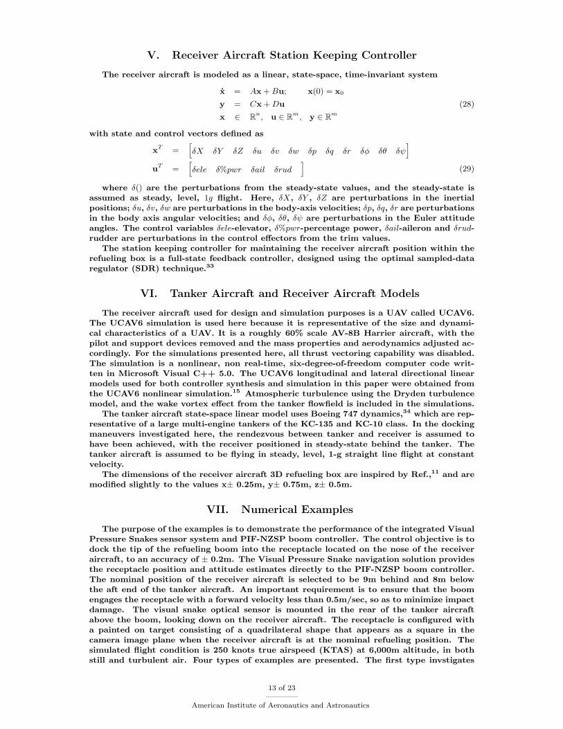
Figure 10 shows the errors resolved in the range and heading directions (with the an-gular heading uncertainty converted to a position uncertainty). Table 4 shows the meanand standard deviations. The error in range greatly dominates the error in heading. Inother words, this visual sensing method determines the target COM heading much moreaccurately than it determines the range to the target. The resulting “measurement errorenvelope” looks like long thin tube, as illustrated in Figure 11. The green lines representthe cone defined by the heading uncertainty, and the red region corresponds to the depthuncertainty. Both regions are extremely exaggerated for effect.

(a) Range Error (b) Position Error from Heading Uncertainty

Figure 10. Range Error, Heading Error, and Heading Position Error for air Refueling Visual Position SensingSimulation.

Table 4. Error Magnitude, Range Error, and Heading Error Data from air Refueling Visual Position SensingSimulation.

Quantity Mean Standard DeviationError Magnitude (m) 0.0124 0.0057

Range Error (m) 6.2919× 10−5 0.0103Heading Error (deg.) 0.0037 0.0020

Position Error from Heading Uncertainty (m) 6.89× 10−4 3.72× 10−4

14 of 23


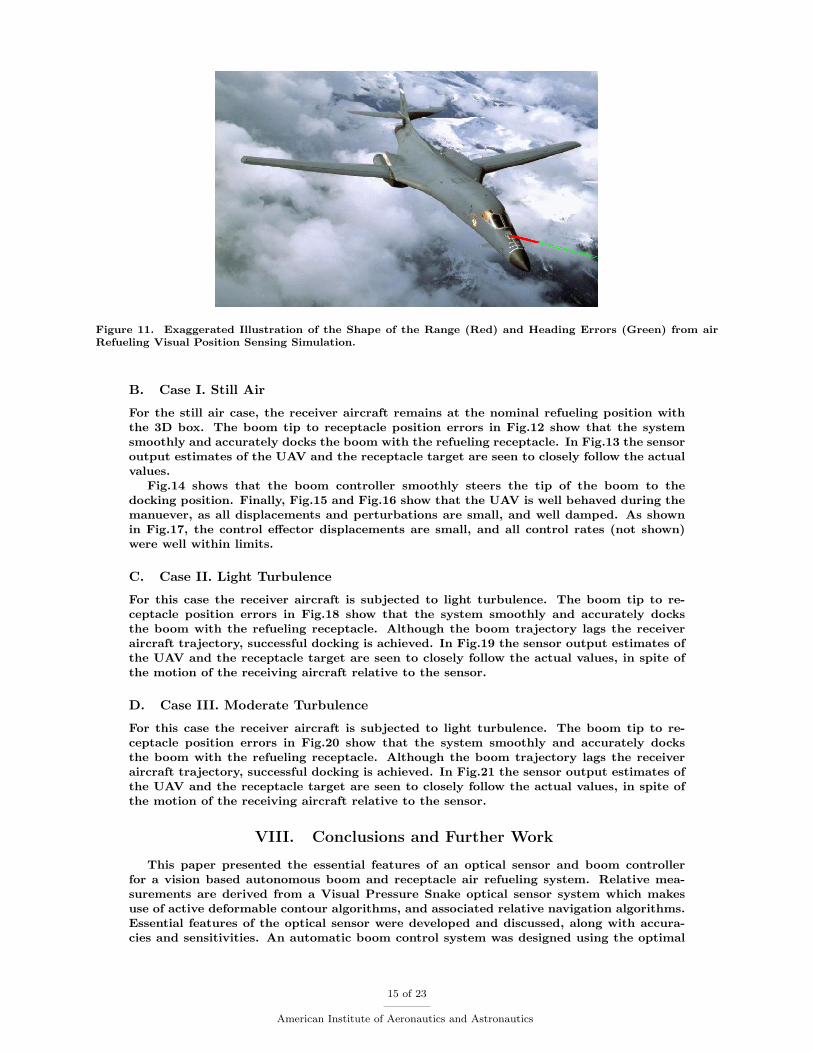
Figure 11. Exaggerated Illustration of the Shape of the Range (Red) and Heading Errors (Green) from airRefueling Visual Position Sensing Simulation.

B. Case I. Still Air

For the still air case, the receiver aircraft remains at the nominal refueling position withthe 3D box. The boom tip to receptacle position errors in Fig.12 show that the systemsmoothly and accurately docks the boom with the refueling receptacle. In Fig.13 the sensoroutput estimates of the UAV and the receptacle target are seen to closely follow the actualvalues.

Fig.14 shows that the boom controller smoothly steers the tip of the boom to thedocking position. Finally, Fig.15 and Fig.16 show that the UAV is well behaved during themanuever, as all displacements and perturbations are small, and well damped. As shownin Fig.17, the control effector displacements are small, and all control rates (not shown)were well within limits.

C. Case II. Light Turbulence

For this case the receiver aircraft is subjected to light turbulence. The boom tip to re-ceptacle position errors in Fig.18 show that the system smoothly and accurately docksthe boom with the refueling receptacle. Although the boom trajectory lags the receiveraircraft trajectory, successful docking is achieved. In Fig.19 the sensor output estimates ofthe UAV and the receptacle target are seen to closely follow the actual values, in spite ofthe motion of the receiving aircraft relative to the sensor.

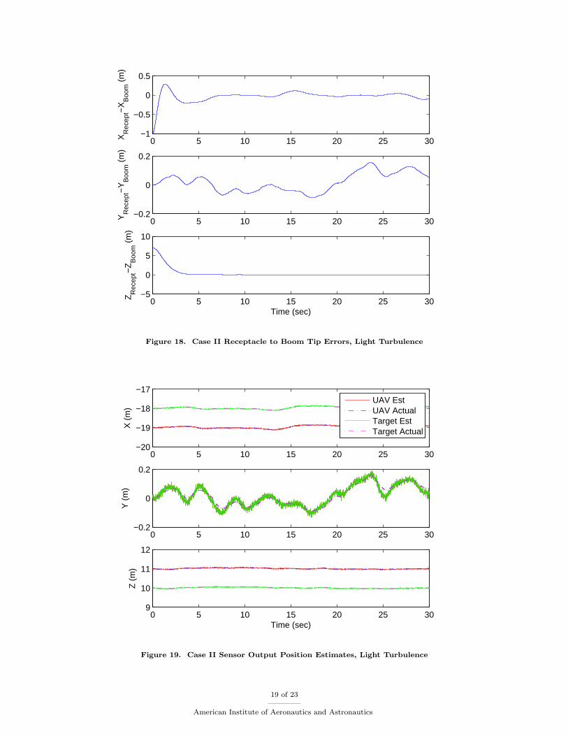
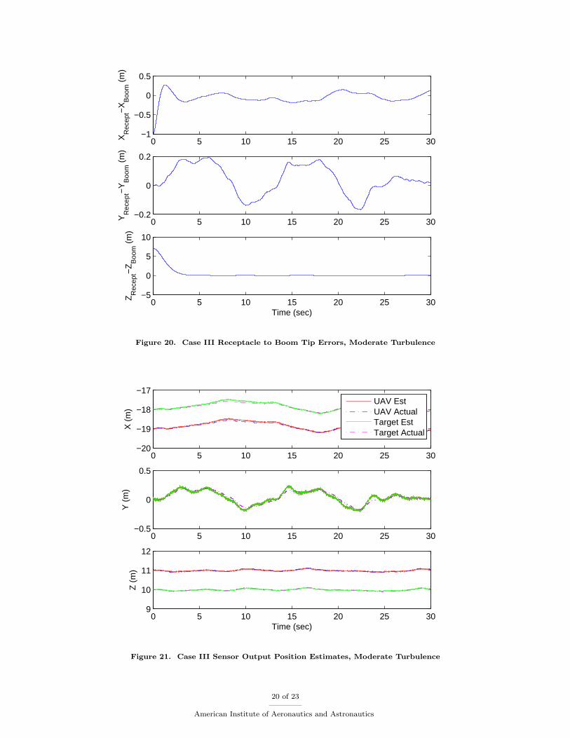
D. Case III. Moderate Turbulence

For this case the receiver aircraft is subjected to light turbulence. The boom tip to re-ceptacle position errors in Fig.20 show that the system smoothly and accurately docksthe boom with the refueling receptacle. Although the boom trajectory lags the receiveraircraft trajectory, successful docking is achieved. In Fig.21 the sensor output estimates ofthe UAV and the receptacle target are seen to closely follow the actual values, in spite ofthe motion of the receiving aircraft relative to the sensor.

VIII. Conclusions and Further Work

This paper presented the essential features of an optical sensor and boom controllerfor a vision based autonomous boom and receptacle air refueling system. Relative mea-surements are derived from a Visual Pressure Snake optical sensor system which makesuse of active deformable contour algorithms, and associated relative navigation algorithms.Essential features of the optical sensor were developed and discussed, along with accura-cies and sensitivities. An automatic boom control system was designed using the optimal

15 of 23


0 5 10 15 20 25 30−1

−0.5

0

0.5

XR

ecep

t−X

Boo

m (

m)

0 5 10 15 20 25 30−0.5

0

0.5

YR

ecep

t−Y

Boo

m (

m)

0 5 10 15 20 25 30−5

0

5

10

ZR

ecep

t−Z

Boo

m (

m)

Time (sec)

Figure 12. Case I Receptacle to Boom Tip Errors, Still Air

0 5 10 15 20 25 30−20

−19

−18

−17

X (

m)

UAV EstUAV ActualTarget EstTarget Actual

0 5 10 15 20 25 30−0.5

0

0.5

Y (

m)

0 5 10 15 20 25 309

10

11

12

Z (

m)

Time (sec)

Figure 13. Case I Sensor Output Position Estimates, Still Air

16 of 23


0 10 20 30−1

0

1

Time(sec)ψ

Boo

m (

deg)

0 10 20 300

50

Time(sec)

θ Boo

m (

deg)

0 10 20 305

10

15

Time(sec)

Leng

thB

oom

(m

)0 10 20 30

−1

0

1

Time(sec)

ψB

oom

dot

(de

g/s)

0 10 20 30−50

0

50

Time(sec)

θ Boo

m d

ot (

deg/

s)0 10 20 30

−2

0

2

Time(sec)

Leng

thB

oom

dot

(m

/s)

Figure 14. Case I Boom Displacement, Rotations, and Rates, Still Air

0 10 20 30127.8

127.9

128

Time(sec)

Vel

ocity

(m

/s)

0 10 20 30−0.05

0

0.05

Time(sec)

β (d

eg)

0 10 20 304

4.5

5

Time(sec)

α (d

eg)

0 10 20 30128.25

128.3

128.35

Time(sec)

u (m

/s)

0 10 20 30−0.1

0

0.1

Time(sec)

v (m

/s)

0 10 20 309.5

10

10.5

Time(sec)

w (

m/s

)

Figure 15. Case I Receiver Aircraft States, Still Air

17 of 23


0 10 20 30−5

0

5

Time(sec)p

(deg

/sec

)

0 10 20 30−1

0

1

Time(sec)

q (d

eg/s

ec)

0 10 20 30−0.5

0

0.5

Time(sec)

r (d

eg/s

ec)

0 10 20 30−2

0

2

Time(sec)

φ (d

eg)

0 10 20 30−0.2

0

0.2

Time(sec)

θ (d

eg)

0 10 20 30−0.2

0

0.2

Time(sec)

ψ (

deg)

Figure 16. Case I Receiver Aircraft Angular States, Still Air

0 10 20 307

7.5

8

8.5

Time(sec)

δ e (de

g)

0 10 20 3054

54.5

55

55.5

Time(sec)

δ T (

%)

0 10 20 30−1

−0.5

0

0.5

1

Time(sec)

δ a (de

g)

0 10 20 30−0.2

0

0.2

0.4

0.6

Time(sec)

δ r (de

g)

Figure 17. Case I Receiver Aircraft Control Effectors, Still Air

18 of 23


0 5 10 15 20 25 30−1

−0.5

0

0.5

XR

ecep

t−X

Boo

m (

m)

0 5 10 15 20 25 30−0.2

0

0.2

YR

ecep

t−Y

Boo

m (

m)

0 5 10 15 20 25 30−5

0

5

10

ZR

ecep

t−Z

Boo

m (

m)

Time (sec)

Figure 18. Case II Receptacle to Boom Tip Errors, Light Turbulence

0 5 10 15 20 25 30−20

−19

−18

−17

X (

m)


0 5 10 15 20 25 30−0.2

0

0.2

Y (

m)

0 5 10 15 20 25 309

10

11

12

Z (

m)

Time (sec)

Figure 19. Case II Sensor Output Position Estimates, Light Turbulence

19 of 23


0 5 10 15 20 25 30−1

−0.5

0

0.5

XR

ecep

t−X

Boo

m (

m)

0 5 10 15 20 25 30−0.2

0

0.2

YR

ecep

t−Y

Boo

m (

m)

0 5 10 15 20 25 30−5

0

5

10

ZR

ecep

t−Z

Boo

m (

m)

Time (sec)

Figure 20. Case III Receptacle to Boom Tip Errors, Moderate Turbulence

0 5 10 15 20 25 30−20

−19

−18

−17

X (

m)


0 5 10 15 20 25 30−0.5

0

0.5

Y (

m)

0 5 10 15 20 25 309

10

11

12

Z (

m)

Time (sec)

Figure 21. Case III Sensor Output Position Estimates, Moderate Turbulence

20 of 23


Proportional-Integral-Filter Nonzero Set Point methodology, which receives relative posi-tion measurements from the optical sensor. Performance and suitability of the system wasdemonstrated with simulated docking maneuvers between a tanker aircraft and a receiverUAV, in various levels of turbulence. Results indicate that the system is able to success-fully accomplish the autonomous refueling task within specifications of docking accuracyand maximum docking velocity. The disturbance accommodation properties of the con-troller in turbulence are judged to be good, and provide a basis for optimism as regards toproceeding toward actual implementation.

Further investigations will determine the optimal visual target pattern, and determinerobustness with respect to off-nominal lighting conditions, additional sensor dynamics, andmeasurement errors. An improved trajectory tracking controller which can more effectivelytrack time varying receptacle position is being developed in parallel, as a precursor to flighttests.

Acknowledgement

The authors wish to thank Theresa Spaeth for development of the air vehicle modelsand simulations.

Appendix

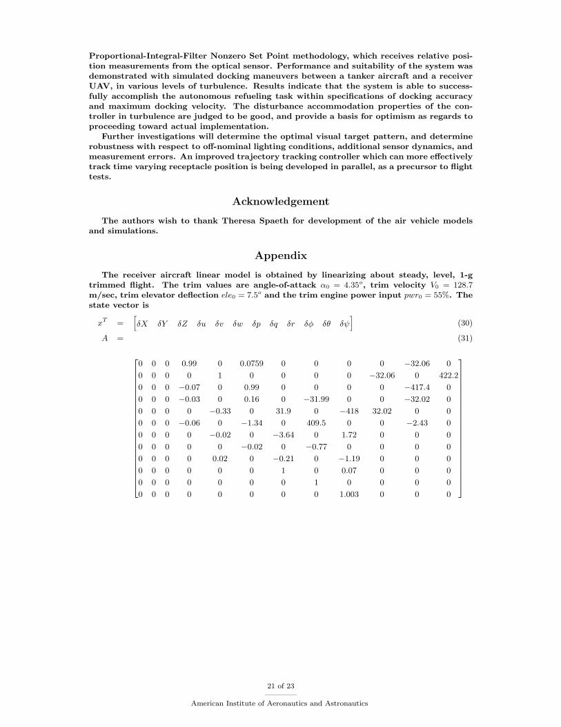
The receiver aircraft linear model is obtained by linearizing about steady, level, 1-gtrimmed flight. The trim values are angle-of-attack α0 = 4.35o, trim velocity V0 = 128.7m/sec, trim elevator deflection ele0 = 7.5o and the trim engine power input pwr0 = 55%. Thestate vector is

xT =[δX δY δZ δu δv δw δp δq δr δφ δθ δψ

](30)

A = (31)

0 0 0 0.99 0 0.0759 0 0 0 0 −32.06 0

0 0 0 0 1 0 0 0 0 −32.06 0 422.2

0 0 0 −0.07 0 0.99 0 0 0 0 −417.4 0

0 0 0 −0.03 0 0.16 0 −31.99 0 0 −32.02 0

0 0 0 0 −0.33 0 31.9 0 −418 32.02 0 0

0 0 0 −0.06 0 −1.34 0 409.5 0 0 −2.43 0

0 0 0 0 −0.02 0 −3.64 0 1.72 0 0 0

0 0 0 0 0 −0.02 0 −0.77 0 0 0 0

0 0 0 0 0.02 0 −0.21 0 −1.19 0 0 0

0 0 0 0 0 0 1 0 0.07 0 0 0

0 0 0 0 0 0 0 1 0 0 0 0

0 0 0 0 0 0 0 0 1.003 0 0 0

21 of 23


The control vector is

uT =[δele δ%pwr δail δrud

](32)

B =

0 0 0 0

0 0 0 0

0 0 0 0

0.0081 0.2559 0 0

0 0 −0.2945 0.4481

0.2772 0.2286 0 0

0 0 0.5171 0.0704

0.1164 0.0143 0 0

0 0 0.0239 −0.0895

0 0 0 0

0 0 0 0

0 0 0 0

(33)

References

1Smith, R. K., “Seventy-Five Years of Inflight Refueling,” Air Force and Museums Program,1998.

2Pennington, R. J., “Tankers,” Air and Space Smithsonian, Vol. 12, No. 4, November 1997,pp. 24–37.

3Maiersperger, W. P., “General Design Aspects of Flight Refueling,” Aeronautical EngineeringReview , Vol. 13, No. 3, March 1954, pp. 52–61.

4Personal Conversation with M. Bandak, Sargent Fletcher Inc., Jan 2002.5Stephenson, J. L., The Air Refueling Receiver That Does Not Complain, Ph.D. thesis, School of

Advanced Airpower Studies Air University, Maxwell Air Force Base, Alabama, June 1998.6Andersen, C. M., Three Degree of Freedom Compliant Motion Control For Robotic Aircraft Re-

fueling , Master’s thesis, Aeronautical Engineering, Air Force Institute of Technology, Wright-Patterson, Ohio, December 13 1990, AFIT/GAE/ENG/90D-01.

7Bennett, R. A., Brightness Invariant Port Recognition For Robotic Aircraft Refueling , Master’sthesis, Electrical Engineering, Air Force Institute of Technology, Wright-Patterson, Ohio, Decem-ber 13 1990, AFIT/GE/ENG/90D-04.

8Shipman, R. P., Visual Servoing For Autonomous Aircraft Refueling , Master’s thesis, Air ForceInstitute of Technology, Wright-Patterson, Ohio, December 1989, AFIT/GE/ENG/89D-48.

9Abidi, M. A. and Gonzalez, R. C., “The Use of Multisensor Data for Robotic Applications,”IEEE Transactions on Robotics and Automation, Vol. 6, No. 2, April 1990, pp. 159–177.

10Lachapelle, G., Sun, H., Cannon, M. E., and Lu, G., “Precise Aircraft-to-Aircraft PositioningUsing a Multiple Receiver Configuration,” Proceedings of the National Technical Meeting, Instituteof Navigation, Inst of Navigation, Alexandria, VA, 1994, pp. 793–799.

11Vendra, S., Addressing Corner Detection Issues for Machine Vision based UAV , Master’s the-sis, College of Engineering and Mineral Resources, West Virginia University, Morgantown, WestVirginia, March 2006, Aerospace Engineering Department.

12Junkins, J. L., Hughes, D., Wazni, K., and Pariyapong, V., “Vision-Based Navigation for Ren-dezvous, Docking, and Proximity Operations,” 22nd Annual ASS Guidance and Control Conference,No. ASS-99-021, Breckenridge, Colorado, February 1999.

13Alonso, R., Crassidis, J. L., and Junkins, J. L., “Vision-Based Relative Navigation for For-mation Flying of Spacecraft,” No. AIAA-2000-4439, American Institute of Aeronautics and Astro-nautics, 2000.

14Gunnam, K., Hughes, D., LJunkins, J., and Nasser, K.-N., “A DSP Embedded Optical Nav-igation System,” Proceedings of the Sixth International Conference on Signal Processing (IC SP ’02),Beijing, People’s Republic of China, August 2002.

15Valasek, J., Gunnam, K., Kimmett, J., Tandale, M. D., Junkins, J. L., and Hughes, D.,“Vision-Based Sensor and Navigation System for Autonomous Air Refueling,” Journal of Guidance,Control, and Dynamics, Vol. 28, No. 5, September-October 2005, pp. 832–844.

16Tandale, M. D., Bowers, R., and Valasek, J., “Vision-Based Sensor and Navigation Systemfor Autonomous Air Refueling,” Journal of Guidance, Control, and Dynamics, Vol. 29, No. 4, July-August 2006, pp. 846–857.

17Valasek, J., Kimmett, J., Hughes, D., Gunnam, K., and Junkins, J. L., “Vision Based Sensorand Navigation System for Autonomous Aerial Refueling,” Proceedings of the AIAA 1st TechnicalConference and Workshop on Unmanned Aerospace Vehicles, Technologies, and Operations, No. AIAA-2002-3441, Portsmouth, Virgina, May 2002.

18Kimmett, J., Valasek, J., and Junkins, J. L., “Autonomous Aerial Refueling Utilizing A VisionBased Navigation System,” Proceedings of the AIAA Guidance, Navigation, and Control Conference,No. AIAA-2002-4469, Monterey, CA, 5-8 August 2002.

19Kimmett, J., Valasek, J., and Junkins, J. L., “Vision Based Controller for Autonomous Aerial

22 of 23


Refueling,” Proceedings of the IEEE Control Systems Society Conference on Control Applications, No.CCA02-CCAREG-1126, Glasgow, Scotland, Sept. 2002.

20Valasek, J. and Junkins, J. L., “Intelligent Control Systems and Vison Based Navigation toEnable Autonomous Aerial Refueling of UAVs,” 27th Annual AAS Guidance and Control Conference,No. AAS 04-012, Breckenridge, CO, Feb. 2004.

21Tandale, M. D., Bowers, R., and Valasek, J., “Robust Trajectory Tracking Controller forVision Based Probe and Drogue Autonomous Aerial Refueling,” Proceedings of the AIAA Guidance,Navigation, and Control Conference, No. AIAA-2005-5868, San Francisco, CA, 15-18 August 2005.

22Tandale, M. D., Valasek, J., and Junkins, J. L., “Vision Based Autonomous Aerial Refuelingbetween Unmanned Aircraft using a Reference Observer Based Trajectory Tracking Controller,”Proceedings of the 2006 American Automatic Control Conference, No. AIAA-2005-5868, Minneapolis,MN, 14-16 June 2006.

23Kass, M., Witkin, A., and Terzopoulos, D., “Snakes: active contour models,” InternationalJournal of Computer Vision, Vol. 1, No. 4, 1987, pp. 321–331.

24Perrin, D. and Smith, C. E., “Rethinking Classical Internal Forces for Active Contour Mod-els,” Proceedings of the IEEE International Conference on Computer Vision and Pattern Recognition,Vol. 2, Dec. 8–14 2001, pp. 615–620.

25Schaub, H. and Smith, C. E., “Color Snakes for Dynamic Lighting Conditions on MobileManipulation Platforms,” IEEE/RJS International Conference on Intelligent Robots and Systems,Las Vegas, NV, Oct. 2003.

26Smith, C. E. and Schaub, H., “Efficient Polygonal Intersection Determination with Applica-tions to Robotics and Vision,” IEEE/RSJ International Conference on Intelligent Robots and Systems,Edmonton, Alberta, Canada, Aug. 2–6 2005.

27Monda, M. and Schaub, H., “Spacecraft Relative Motion Estimation using Visual SensingTechniques,” AIAA Infotech@Aerospace Conference, Arlington, VA, Sept. 26–29 2005, Paper No.05-7116.

28Kass, M., Witkin, A., and Terzopoulos, D., “Snakes: Active contour models,” InternationalJournal of Computer Vision, Vol. 1, No. 4, 1987, pp. 321–331.

29Perrin, D. P., Ladd, A. M., Kavraki, L. E., Howe, R. D., and Cannon, J. W., “Fast IntersectionChecking for Parametric Deformable Models,” SPIE Medical Imaging , San Diego, CA, February 12–17 2005.

30Malladi, R., Kimmel, R., Adalsteinsson, D., Sapiro, G., Caselles, V., and Sethian, J. A., “Ageometric approach to segmentation and analysis of 3D medical images,” Proceedings of Mathemat-ical Methods in Biomedical Image Analysis Workshop, San Francisco, June 21–22 1996.

31Ivins, J. and Porrill, J., “Active Region Models for Segmenting Medical Images,” Proceedingsof the IEEE International Conference on Image Processing , Austin, Texas, 1994, pp. 227–231.

32Schaub, H. and Wilson, C., “Matching a Statistical Pressure Snake to a Four-Sided Poly-gon and Estimating the Polygon Corners,” Technical Report SAND2004-1871, Sandia NationalLaboratories, Albuquerque, NM, 2003.

33Dorato, P., “Optimal Linear Regulators: The Discrete-Time Case,” IEEE Transactions onAutomatic Control , Vol. AC-16, No. 6, December 1971, pp. 613–620.

34Roskam, J., Airplane Flight Dynamics and Automatic Flight Controls, Part I , Vol. 1, Design,Analysis, and Research Corporation, Lawrence, KS, 1994, p. 236.

23 of 23


Documents

Boom and Receptacle Autonomous Air Refueling Using …dnc.tamu.edu/projects/smartsensors/papers/archival/JGCDandAIAA... · Boom and Receptacle Autonomous Air Refueling Using a Visual