Fast 3D Viscous Calculation Methods

Mark DrelaMIT Aero & Astro

Boeing/MIT Strategic Research Review6 May 14

Motivation

2D Inviscid+Integral-BL (IBL) methods have proven very effective

• Enormously faster than alternative Navier-Stokes for similar accuracy

• Can exploit any inviscid flow solver

• Compatible with inverse design methods

• Compatible with virtual displacements for linearized aeroelasticity

Navier Stokes

∼ 500 000 variables∼ 1 hr. runtime

Potential+BL (MSIS, TRANAIR-2D)

∼ 5 000 variables∼ 1 sec. runtime

⇒ Present goal is to extend inviscid+integral-BL methods to 3D

1/23

EIF/Defect Formulation

• Real flow decomposed into irrotational Equivalent Inviscid Flow qi

and rotational Viscous Defect ∆q, with . . .

– qi = q outside the rotational viscous layers

– qi · n 6= 0 on solid walls, accounts for presence of viscous layer

(qi is not the solution to the inviscid problem!)

RealViscous Flow i

( )r

( )r

( )rq

q

q∆ qi q−

EIF

Viscous Defect

iq n 0.EIF Wall BC:

qi q=

q = 0Wall BC:( EIF wall mass flux depends on integrated defect )

nn

• Originally employed by LeBalleur with boundary layer methods,but EIF/Defect formulation does not depend on BL approximations

2/23

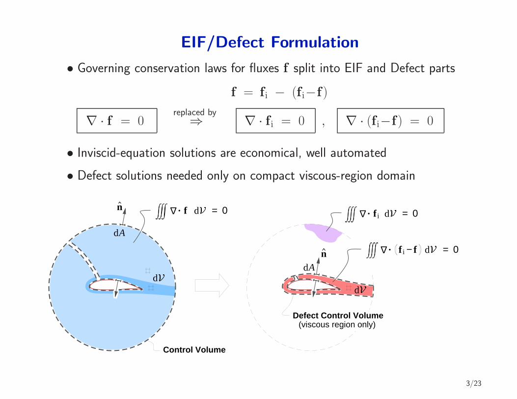
EIF/Defect Formulation

• Governing conservation laws for fluxes f split into EIF and Defect parts

f = fi − (fi−f)

∇ · f = 0replaced by

⇒ ∇ · fi = 0 , ∇ · (fi−f) = 0

• Inviscid-equation solutions are economical, well automated

• Defect solutions needed only on compact viscous-region domain

Control Volume

Defect Control Volume(viscous region only)

n

n

dd

Ad

Ad

. f d

∆ = 0

. −i ff d

∆ = 0

. f

∆ = 0i d

3/23

EIF/Defect Formulation

Defect conservation law on differential volume spanning viscous layer

∫∫∫∇· (fi−f) dV =

∫∫ ˜∇ ·[∫ yeyw

(

f i− f)

dy]

dx dz

+∫∫(fi−f)e · ne dAe

−∫∫(fi−f)w · nw dAw = 0

where f = fx x + fz z (in-plane flux)˜∇() = ∂()

∂x x + ∂()∂z z (in-plane gradient)

Defect Control Volume

Differential Defect Control Volume

...

... ...

......... ...

...

exit

n

n

y ( )x,ze

y ( )x,zw

ne

nw

w

e

A

x

Ad

d

d

dz

y,υ

x,z , u,w

4/23

Defect EquationsDefect equations on differential volumes spanning viscous layer

∫(mass i − mass) dy → ˜∇·M− ρiwqiw·nw = 0

∫(momi−mom) dy → ˜∇· ¯J − ˜∇·Mqiw − τw − (piw−pw)nw + ˜∇Π = 0

∫(qi · momi−q · mom) dy → ˜∇·E − ˜∇·M q2iw − ρiQ· ˜∇q2i − 2D = 0

∫(qi×momi−q×mom)·y dy → ˜∇·E◦− ˜∇·M q2iwψiw − ρiQ

◦· ˜∇q2i . . .− 2D◦ = 0

Conserved integral defects (fluxes), source terms

M ≡∫(ρiqi − ρq) dy Mass flux defect

¯J ≡∫(ρiqi q

Ti − ρqqT) dy Momentum flux defect

E ≡∫(ρiqi q

2i − ρq q2) dy K.E. flux defect

E◦ ≡∫(ρiqi q

2i ψi − ρq q2ψ) dy Curvature flux defect

Q ≡∫(qi − q) dy Volume flux defect

Π ≡∫(pi − p) dy Pressure defect

D ≡∫( ¯τ ·∇) · q dy Dissipation integral

...

iqρiqρ

iq n.ρwiw w

M J E, , E, ...=τττw

In-plane flow angle variable: ψ(y) ≡ arctan(w/u)5/23

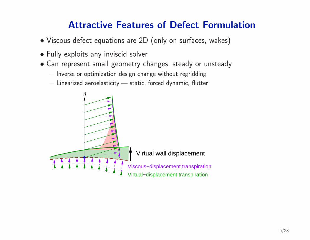
Attractive Features of Defect Formulation

• Viscous defect equations are 2D (only on surfaces, wakes)

• Fully exploits any inviscid solver• Can represent small geometry changes, steady or unsteady

– Inverse or optimization design change without regridding

– Linearized aeroelasticity — static, forced dynamic, flutter

n

Virtual wall displacement

Virtual−displacement transpiration

Viscous−displacement transpiration

6/23

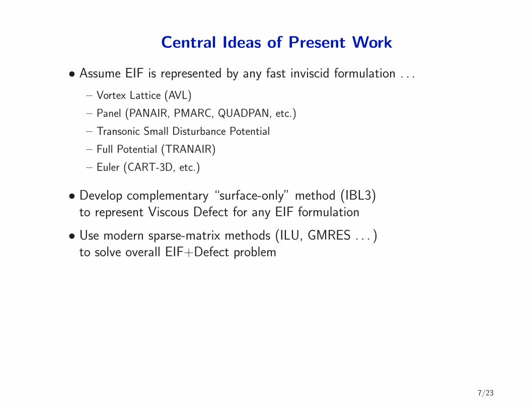
Central Ideas of Present Work

• Assume EIF is represented by any fast inviscid formulation . . .

– Vortex Lattice (AVL)

– Panel (PANAIR, PMARC, QUADPAN, etc.)

– Transonic Small Disturbance Potential

– Full Potential (TRANAIR)

– Euler (CART-3D, etc.)

• Develop complementary “surface-only” method (IBL3)to represent Viscous Defect for any EIF formulation

• Use modern sparse-matrix methods (ILU, GMRES . . . )to solve overall EIF+Defect problem

7/23

IBL3 Formulation

• Viscous defects represented by assumed profiles, parameterized by

δ A B Ψ (roughly equivalent to δ∗1 θ11 δ∗2 θ12)

• TS, CF-wave amplitudes and Reynolds stresses parameterized by

GC ψC

(

equivalent to ln[

u′12+u′2

2]

, arctan[

‖u′2‖/‖u′1‖

])

• Enormous reduction in number of unknowns from RANS

n

Viscous Defects(mass, mom., KE)

Navier Stokes

RealViscous Flow

i

Potential solvergrid resolutionrequired for( )rq q

i( )rq

EIF

δ Ψρ ρq ρe( ) j

j

Typical required Navier−Stokes grid resolution

6 DOFs per surface point

ν

200 to 600 DOFs per surface point

IBL3

ψGC C

8/23

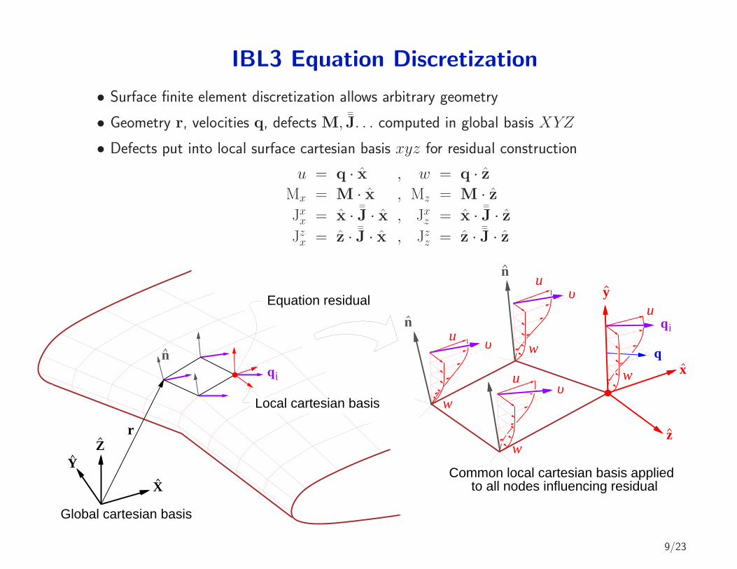
IBL3 Equation Discretization

• Surface finite element discretization allows arbitrary geometry

• Geometry r, velocities q, defects M, ¯J. . . computed in global basis XYZ

• Defects put into local surface cartesian basis xyz for residual construction

u = q · x , w = q · z

Mx = M · x , Mz = M · z

Jxx = x · ¯J · x , Jxz = x · ¯J · z

Jzx = z · ¯J · x , Jzz = z · ¯J · z

X

ZY

Global cartesian basis

Local cartesian basis

r

u

w x

z

q

q

i

y

n

n

u

w

w

u

u

w

qi

nυ

υ

υEquation residual

Common local cartesian basis applied to all nodes influencing residual

9/23

IBL3 Solution Approach

Finite-element discretization in local surface xyz basis

• Greatly simplified solution logic – no need to identify attachment lines, stag-nation points

• Simple Dirichlet, Neumann PCs – no edge stencils needed

• Compatible with simultaneous solution with inviscid flow

N

NN

N

−1+1 −1

+1

1

2

3

4

ζ ξ

ζ

ξ

x

z

ξ

ζ1 2

34

n

n

iW iW

iW

n

n

nS

S

S

S

S

10/23

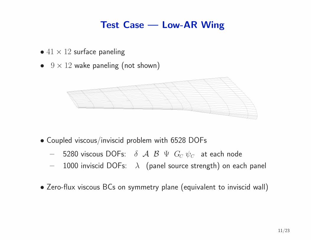
Test Case — Low-AR Wing

• 41× 12 surface paneling

• 9× 12 wake paneling (not shown)

• Coupled viscous/inviscid problem with 6528 DOFs

– 5280 viscous DOFs: δ A B Ψ GC ψC at each node

– 1000 inviscid DOFs: λ (panel source strength) on each panel

• Zero-flux viscous BCs on symmetry plane (equivalent to inviscid wall)

11/23

Test Case — Low-AR Wing

EIF and wall streamlines for laminar flow at Re = 40 000

α = 0.0° EIF streamlines

Skin friction lines

α = 4.0°

57% span

EIF streamlines

Skin friction lines

⇒ Separation lines are naturally captured within IBL3 surface grid

12/23

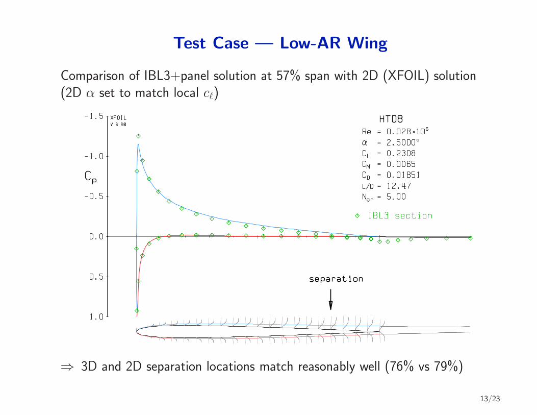
Test Case — Low-AR Wing

Comparison of IBL3+panel solution at 57% span with 2D (XFOIL) solution(2D α set to match local cℓ)

⇒ 3D and 2D separation locations match reasonably well (76% vs 79%)

13/23

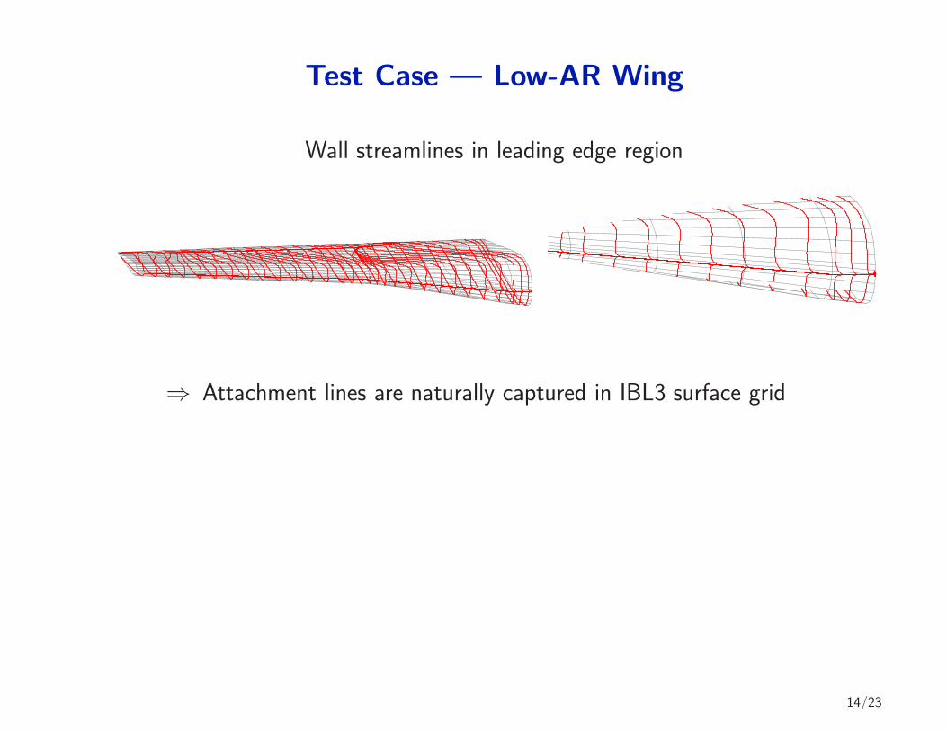
Test Case — Low-AR Wing

Wall streamlines in leading edge region

⇒ Attachment lines are naturally captured in IBL3 surface grid

14/23

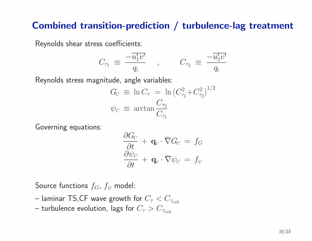
Combined transition-prediction / turbulence-lag treatment

Reynolds shear stress coefficients:

Cτ1 ≡−u′1v

′

qi, Cτ2 ≡

−u′2v′

qi

Reynolds stress magnitude, angle variables:

GC ≡ lnCτ = ln(C2τ1+C2

τ2

)1/2

ψC ≡ arctanCτ2Cτ1

Governing equations:∂GC

∂t+ qc ·

˜∇GC = fG

∂ψC

∂t+ qc ·

˜∇ψC = fψ

Source functions fG, fψ model:

– laminar TS,CF wave growth for Cτ < Cτcrit– turbulence evolution, lags for Cτ > Cτcrit

15/23

Torpedo Test Case

“Torpedo” over a wall boundary layer

qSourceLeading edge

"Torpedo"

"Torpedo"

Computational grid

Side View

Inflow edge

Inflow edge

Outflow edge

16/23

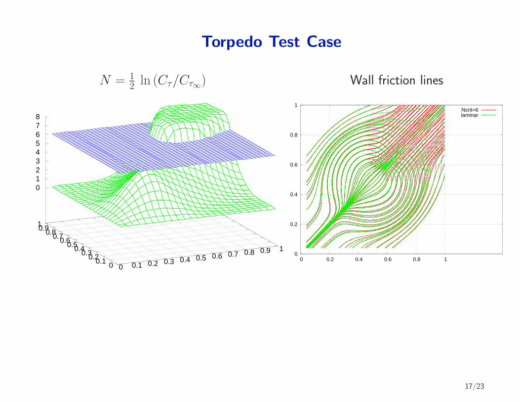
Torpedo Test Case

N = 12 ln (Cτ/Cτ∞) Wall friction lines

0 0.1 0.2 0.3 0.4 0.5 0.6 0.7 0.8 0.9 1

0 0.1 0.2 0.3 0.4 0.5 0.6 0.7 0.8 0.9 1

0 1 2 3 4 5 6 7 8

0

0.2

0.4

0.6

0.8

1

0 0.2 0.4 0.6 0.8 1

Ncrit=6laminar

17/23

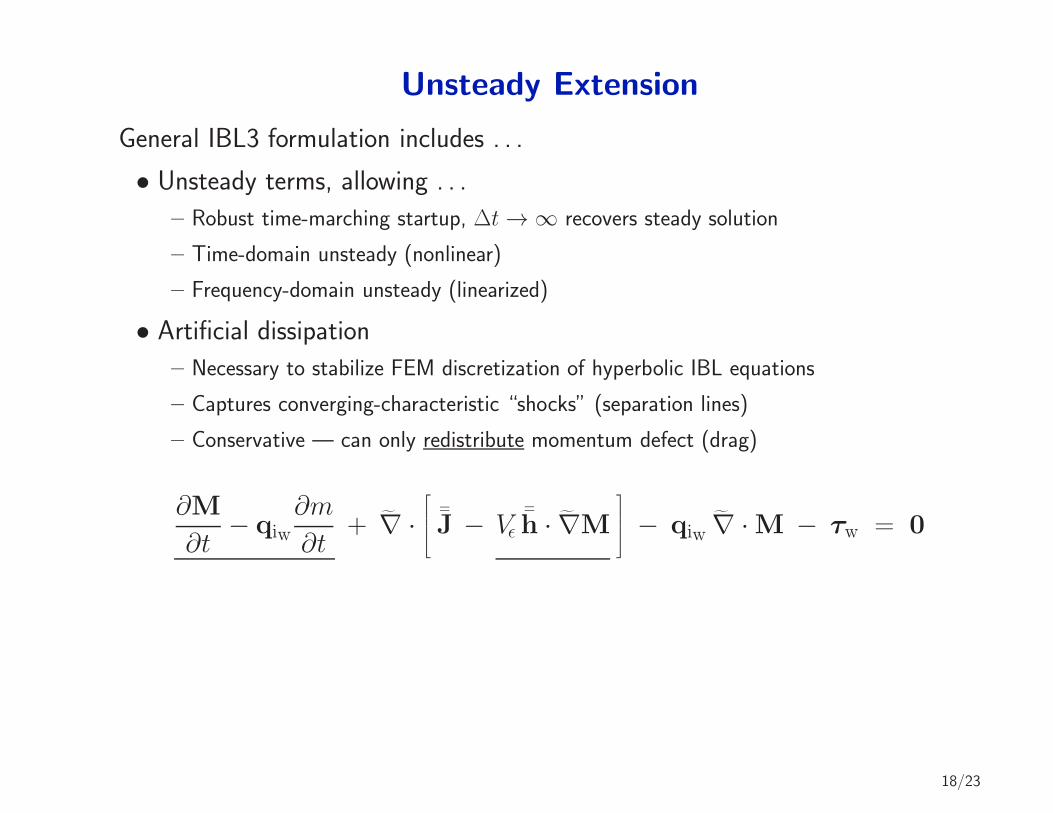
Unsteady Extension

General IBL3 formulation includes . . .

• Unsteady terms, allowing . . .

– Robust time-marching startup, ∆t→ ∞ recovers steady solution

– Time-domain unsteady (nonlinear)

– Frequency-domain unsteady (linearized)

• Artificial dissipation

– Necessary to stabilize FEM discretization of hyperbolic IBL equations

– Captures converging-characteristic “shocks” (separation lines)

– Conservative — can only redistribute momentum defect (drag)

∂M

∂t− qiw

∂m

∂t+ ˜∇ ·

¯J − Vǫ

¯h · ˜∇M

− qiw

˜∇ ·M − τw = 0

18/23

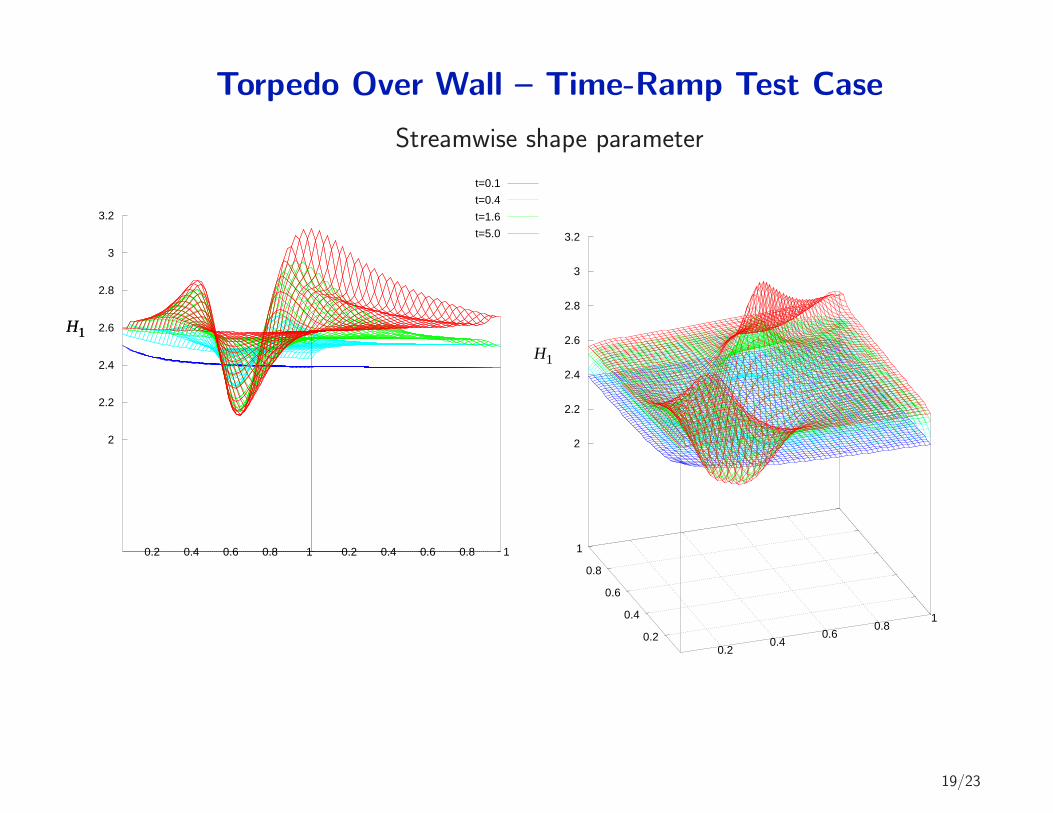
Torpedo Over Wall – Time-Ramp Test Case

Streamwise shape parameter

0.2 0.4 0.6 0.8 1 0.2 0.4 0.6 0.8 1

2

2.2

2.4

2.6

2.8

3

3.2

H1

t=0.1

t=0.4

t=1.6

t=5.0

H1

0.2 0.4

0.6 0.8

1

0.2

0.4

0.6

0.8

1

2

2.2

2.4

2.6

2.8

3

3.2

H1

19/23

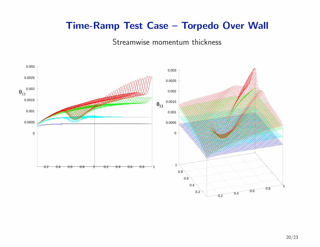
Time-Ramp Test Case – Torpedo Over Wall

Streamwise momentum thickness

0.2 0.4 0.6 0.8 1 0.2 0.4 0.6 0.8 1

0

0.0005

0.001

0.0015

0.002

0.0025

0.003

θ11

0.2 0.4

0.6 0.8

1

0.2

0.4

0.6

0.8

1

0

0.0005

0.001

0.0015

0.002

0.0025

0.003

θ11θ11

20/23

IBL3 Work Done to Date

• Development of FE discretization on general surface grids

• Full unsteady implementation

• Laminar closure method

• Envelope-eN 3D transition prediction method

• Development of turbulent closure method

• Combined laminar/transition/turbulent method

• IBL3 1.01 Routine Package, Documentation

• Strong coupling with simple inviscid solver (done)

• Paper: “Three-Dimensional Integral Boundary Layer Formulation for GeneralConfigurations”, 21st AIAA CFD Conference, San Diego, June 2013.

21/23

IBL3 Work Underway or Planned

• Continue testing, calibration

• Better wake treatment

• Implementation into TSD code (Drela, Sato)

• Implementation into TRANAIR (by Boeing)

22/23

People

• MIT:

– Mark Drela (IBL3, EIF coupling)

– PhD student David Moro (VGNS)

– Bob Haimes (geometry)

• Boeing:

– Dave Young & TRANAIR group

– Sho Sato (TSD code)

23/23