Bod Methods Best

DETERMINATION OF BOD KINETIC PARAMETERS AND

EVALUATION OF ALTERNATE METHODS

A Thesis submitted to

THAPAR INSTITUTE OF ENGINEERING & TECHNOLOGY, PATIALA

in partial fulfillment of the requirements for the award of degree of

MASTER OF ENGINEERING

in

ENVIRONMENTAL ENGINEERING

by

BALWINDER SINGH

Under the supervision of

Dr. ANITA RAJOR Dr. A. S. REDDY

DEPARTMENT OF BIOTECHNOLOGY & ENVIRONMENTAL SCIENCES THAPAR INSTITUTE OF ENGINEERING & TECHNOLOGY

(DEEMED UNIVERSITY) PATIALA – 147 004

June, 2004

CERTIFICATE This is to certify that the thesis entitled, “ Determination of BOD Kinetic Parameters

And Evaluation of Alternate Methods” submitted by Balwinder Singh in partial

fulfillment of the requirements for the award of Degree of MASTER OF

ENGINEERING in ENVIRONMENTAL ENGINEERING to Thapar Institute of

Engineering & Technology (Deemed University), Patiala, is a record of student’s own

work carried out by him under our supervision and guidance. The report has not been

submitted for the award of any other degree or certificate in this or any other

university or institute.

(Dr. Anita Rajor) (Dr. A. S. Reddy)

Department of Biotech. & Env. Sciences, Thapar Institute of Engg. & Tech., Patiala – 147004

Lecturer (Selection Grade) Department of Biotech. & Env. Sciences, Thapar Institute of Engg. & Tech., Patiala – 147004

(Dr. Sunil Khanna) (Dr. D. S. Bawa)

Professor & Head, Department of Biotech. & Env. Sciences, Thapar Institute of Engg. & Tech., Patiala – 147004

Dean (Academic Affairs), Thapar Institute of Engg. & Tech., Patiala – 147004

DECLARATION

I here by declare, that the thesis report entitled, “Determination of BOD Kinetic

Parameters And Evaluation of Alternate Methods” written and submitted by me to

Thapar Institute of Engineering & Technology (Deemed University), Patiala, in

partial fulfillment of the requirements for the degree of MASTER OF

ENGINEERING in ENVIRONMENTAL ENGINEERING. This is my original

work & conclusions drawn are based on the material collected by me.

I further declare that this work has not been submitted to this or any other university

for the award of any other degree, diploma or equivalent course.

BALWINDER SINGH

ACKNOWLEDGEMENT

I wish to express my deep gratitude to Dr. A. S. Reddy, Lecturer (Selection Grade),

Department of Biotech. & Environmental Sciences, Thapar Institute of Engg. &

Technology, Patiala for his invaluable guidance, inspiration, valuable suggestions,

encouragement during the entire period of present study. I will not hesitate to express

sincere thanks to Dr. Anita Rajor for providing the constant encouragement and

making the lab work possible under her able guidance.

I am highly thankful to Dr. Sunil Khanna, Head, Department of Biotech. &

Environmental Science for granting permission for the use of departmental labs.

Lastly, I am thankful to my colleagues, friends and family members for bearing with

me and providing me all moral help during the entire period of my work.

BALWINDER SINGH

CONTENTS

CONTENTS PAGE. NO.

Certificate i

Acknowledgement ii

Declaration iii

List of tables iv

List of Figures v

Chapter: 1 Introduction

1.1 Background information and objectives of the study

1.2 Overview of the contents of the report

1.3 Importance of the study

1 – 5

Chapter: 2 Literature Review 6 – 11

Chapter: 3 Materials and Methods 12 – 33

3.1 Introduction

3.2 Sampling

3.3 Serial BOD testing

3.4 Estimation of BOD kinetic parameters

3.4.1 Method of Moments

3.4.2 Least Squares Methods

3.4.3 Thomas Graphical Method

3.4.5 Iteration Method

3.4.6 Fujimoto Method

3.5 comparison of different methods of estimation

CONTENTS PAGE. NO.

Chapter: 4 Results & Discussion

4.1 Introduction

4.2 Results

4.3 Evaluation of methods

4.4 Discussion

4.5 Conclusion

34 - 61

Chapter: 5 Conclusion 62 - 63

References 64 - 66

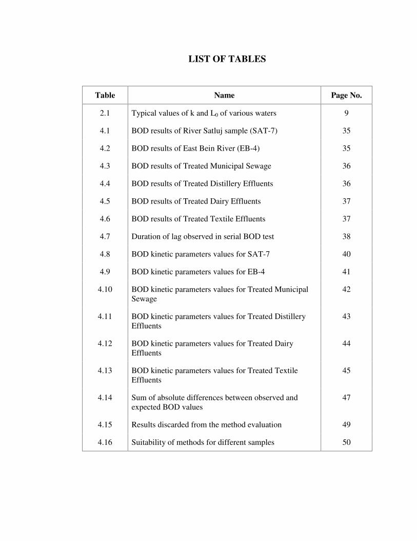
LIST OF TABLES

Table Name Page No.

2.1 Typical values of k and L0 of various waters 9

4.1 BOD results of River Satluj sample (SAT-7) 35

4.2 BOD results of East Bein River (EB-4) 35

4.3 BOD results of Treated Municipal Sewage 36

4.4 BOD results of Treated Distillery Effluents 36

4.5 BOD results of Treated Dairy Effluents 37

4.6 BOD results of Treated Textile Effluents 37

4.7 Duration of lag observed in serial BOD test 38

4.8 BOD kinetic parameters values for SAT-7 40

4.9 BOD kinetic parameters values for EB-4 41

4.10 BOD kinetic parameters values for Treated Municipal Sewage

42

4.11 BOD kinetic parameters values for Treated Distillery Effluents

43

4.12 BOD kinetic parameters values for Treated Dairy Effluents

44

4.13 BOD kinetic parameters values for Treated Textile Effluents

45

4.14 Sum of absolute differences between observed and expected BOD values

47

4.15 Results discarded from the method evaluation 49

4.16 Suitability of methods for different samples 50

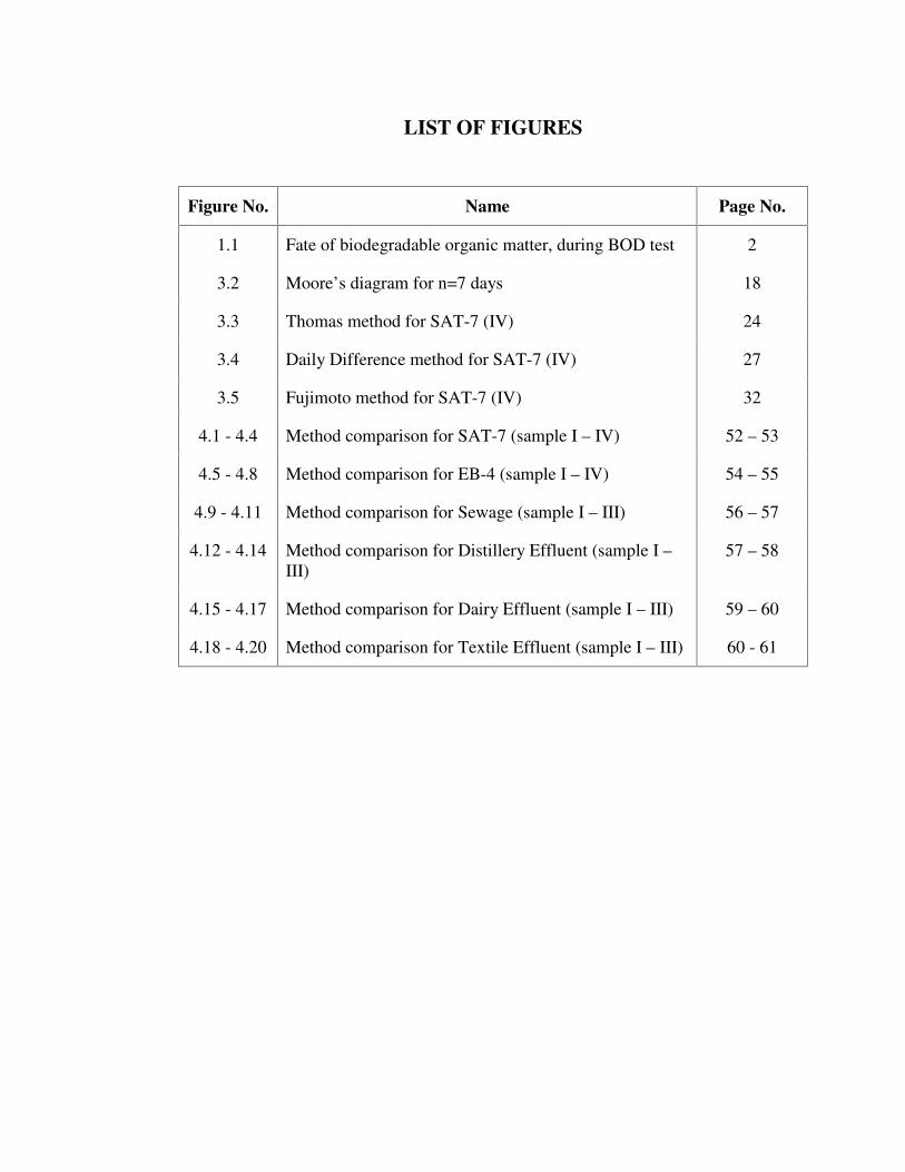
LIST OF FIGURES

Figure No. Name Page No.

1.1 Fate of biodegradable organic matter, during BOD test 2

3.2 Moore’s diagram for n=7 days 18

3.3 Thomas method for SAT-7 (IV) 24

3.4 Daily Difference method for SAT-7 (IV) 27

3.5 Fujimoto method for SAT-7 (IV) 32

4.1 - 4.4 Method comparison for SAT-7 (sample I – IV) 52 – 53

4.5 - 4.8 Method comparison for EB-4 (sample I – IV) 54 – 55

4.9 - 4.11 Method comparison for Sewage (sample I – III) 56 – 57

4.12 - 4.14 Method comparison for Distillery Effluent (sample I – III)

57 – 58

4.15 - 4.17 Method comparison for Dairy Effluent (sample I – III) 59 – 60

4.18 - 4.20 Method comparison for Textile Effluent (sample I – III) 60 - 61

CHAPTER: 1

Introduction

1.1 Background information and objectives of the study:

Biodegradable organic matter is one of the important pollution parameter for water

and wastewater. Being heterogeneous (suspended colloidal and dissolved forms) and

being composed of a wide variety of compounds, it is very difficult to have a single

direct method for estimating its organic matter concentration in any water or

wastewater sample. Because of this reason, indirect methods, like BOD, COD, etc.

are dependent upon for the measurement of organic matter concentration. These

methods measure the organic matter concentration through estimating the amount of

oxygen required for its complete oxidation.

Methods like COD are quite accurate and take very less time for estimating the

organic matter concentration. But they cannot differentiate biodegradable organic

matter from non-biodegradable organic matter. Further, COD is not capable of

accurately estimating volatile organic matter and organic matter with nitrogen bases.

Because of these reasons, BOD is preferred over COD.

In the BOD test microorganisms are used for bio-oxidation of the organic matter in

the presence of oxygen. The amount of oxygen utilized in the bio-oxidation process is

measured and expressed as organic matter concentration in terms of oxygen. This

method actually estimates the amount of biodegradable organic matter rather than the

total organic matter present in water or wastewater sample. In this method, the sample

is diluted to appropriate level, seeded with sufficiently acclimatized microbial

populations, aerated and then filled in the air proof BOD bottles and incubated under

favaourable conditions. Through measuring the initial and final dissolved oxygen

present in the incubated sample, the amount of oxygen consumed in the bio-oxidation

process is estimated. Fig.1.1 shows the fate of biodegradable organic matter during

the incubation in the BOD test.

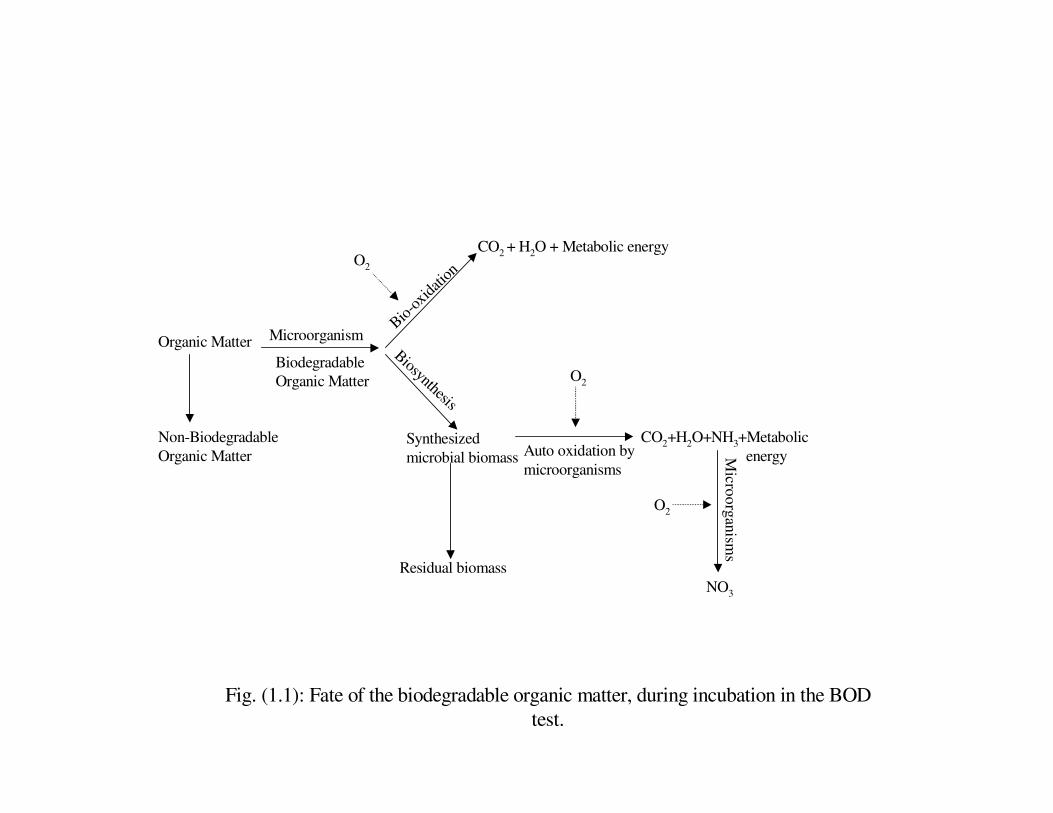
Fig. (1.1): Fate of the biodegradable organic matter, during incubation in the BOD test.

Organic Matter

Non-Biodegradable Organic Matter

Microorganism

Biodegradable Organic Matter

Synthesized microbial biomass

Residual biomass

CO2+H2O+NH3+Metabolic energy

NO3

O2

Microorganism

s

O2

Auto oxidation bymicroorganisms

CO2 + H2O + Metabolic energyO2

Bio-ox

idatio

n

Biosynthesis

The bio-oxidation process is rather slow and complete bio-oxidation takes a quite

long time (over 25 days). This necessitates incubation of the sample for quite long

time for getting the total biodegradable organic matter concentration. In practice,

incubating the sample, for such a long time, is not feasible and even if feasible, since

the results cannot be real time measurements; their utility is very limited. To avoid

this long incubation period a compromising approach is followed. In this approach

the sample is incubated for relatively short period of 5 days for getting major portion

of the organic matter bio-oxidized. The obtained results are extrapolated through

using a mathematical model [BOD kinetics model, y = L0 (1-e-kt)]. Use of this BOD

kinetics model requires prior knowledge of the BOD kinetic parameters (k & L0). The

required kinetic parameters for the water or wastewater in question are obtained

through laboratory experimentation (through conducting serial BOD test, wherein the

BOD exerted of the incubated sample is measured at regular intervals). Results of the

serial BOD test are used in estimating kinetics parameters with the help of one of the

multitude methods available.

Accuracy and reproducibility of BOD testing is not very satisfactory. Hence

estimation of the kinetic parameters which uses serial BOD test results is prone to

become much more inaccurate. For getting satisfactory results selection of

appropriate method of calculation of kinetic parameters is very important. Present

study is actually concerned with evaluation of the commonly used alternative

methods of kinetic parameters estimation. In the present study the following six

methods have actually been evaluated:

1. Method of Moments

2. Method of Least Squares

3. Thomas Graphical Method

4. Daily Difference Method

5. Iteration Method

6. Fujimoto Method

For evaluating these methods, results are obtained from serial BOD testing for 7 days,

of the following samples have been used:

1. Satluj river water sample

2. East Bein river water sample

3. Treated Municipal sewage sample

4. Treated Distillery effluent

5. Treated Dairy effluent

6. Treated Textile effluent

1.2 Overview of the contents of the report:

This M.E. dissertation includes five chapters. Chapter 1 is introduction. In this

chapter after giving brief background information on BOD and BOD kinetics,

objective of the study is introduced. This chapter also includes overview of the

contents of the thesis and importance of the present study.

In Chapter 2, review of published literature on BOD, BOD kinetics and methods for

BOD kinetic parameters estimation is presented.

In the Chapter 3, the approach followed for achieving the objective of the study is

presented. In addition to this, this chapter also includes a brief overview on the

commonly used methods of BOD kinetic parameters estimation.

Chapter 4 includes the results of the study and discussion. The results mainly include

three components, the serial BOD test results, the estimated BOD kinetic parameters,

and results of evaluation of the alternate methods of kinetic parameters estimation. In

the discussion, it has been shown, which of the method is most appropriate and why.

The report concludes with Chapter 5, wherein the study is summarized, limitations of

the study are highlighted and scope for further study is brought forward.

1.3 Importance of the study:

Design, operation and control of biological treatment units require knowledge of

ultimate BOD whereas the BOD test gives 5 days BOD value or 3 days BOD value.

BOD tests are usually conducted at 20ºC, whereas temperature in the biological

treatment units can be different. These situations make BOD kinetics and BOD

kinetic parameters estimation very important. Very few laboratories actually perform

BOD kinetic parameters studies and ultimate BOD is found through thumb rules,

which is undesirable. In the light of these, the present study proves very important.

The study brings about the fact that all methods of kinetic parameters estimation

cannot be appropriate for all conditions. One has to sensibly select appropriate

methods for estimating the kinetic parameters.

CHAPTER: 2

Literature Review

An attempt has been made to review the available literature on BOD, BOD kinetics

and available methods for kinetic parameters estimation. In the nineteenth century the

performance of sewage treatment plants was measured mainly by the chemical

analysis related to the determination of various forms of nitrogen; as an index of the

state and progress of the oxidation of organic matter. Frankland, 1868 as referred by

William (1971) first observed that depletion of dissolved oxygen in the wastewater

containing organic matter was due to chemical reactions. He observed that depletion

of oxygen was dependent on the time of storage. Dupret 1884 as referred by William

(1971) recognized that oxygen depletions were due to the activity of microorganisms.

The classical equation for expressing the BOD process is:

Substrate + bacteria + O2 + growth factors �&22 . H2O + increased

bacteria + energy -------------------------------------------------------------(2.1)

The royal commission on Sewage Disposal, 1912, chose an incubation period of five

days for the BOD test because that is the longest flow time of any British river to the

open sea. An incubation temperature of 20oC was chosen because the long-term

average summer temperature in Britain was 18.3oC (Nesarathnam,1998).

Adeney 1928 as referred by Jenkins (1960) defined the absolute strength of sewage as

the amount of dissolved oxygen required for its complete biochemical oxidation.

Winkler’s method was mostly used to determine the dissolved oxygen content in

water (Standard Method 1995). Bruce et.al, (1993) suggested headspace biochemical

oxygen demand (HBOD) test having three main advantages: the test does not require

sample dilution, oxygen demand determined with in a shorter period of time (24-

36hrs) that can be used predict 5-day BOD value and the experimental conditions

used in the HBOD test, more accurately reproduce the hydrodynamic and culture

conditions. Booki et.al, (2004) suggested the use of fibre optic probe to obtain oxygen

demands in 2 or 3 days in respirometric tests, and then 5-day BOD can be predicted

from the results.

While a standard BOD test procedure developed for certain effluents has been widely

accepted, disagreements regarding the basic mechanisms and kinetics of the test

continue to persist. In fact, a review of the history of the BOD test and the related

mathematical procedures leads to the conclusion that the only universally accepted

concept is that the basic reactions involved are biochemical in nature. The

controversies about BOD kinetics arises largely due to the fact that the distinction

between BOD as a test and BOD as a microbial metabolic process is frequently

overlooked. (The term process is used to refer to the series of cellular enzymatic

reactions, which bring about the conversion of given reactants to final products under

the constraints of the prevalent environmental constraints and factors)(William

E.1971).

Phelps (1953) has presented the developmental history of BOD test and its kinetics.

He after studying the simplified reaction system associated with eq. 2.1 suggested that

the velocity of the reaction varied directly as the concentration of the bacterial food

supply (substrate). The concentration of the substrate was rated in terms of oxygen

equivalents as indicated by the test. Nonetheless, Phelps realized the limitations of his

empirical monomolecular law and delineated them quite clearly. In essence, he

concluded that though there was no actual reason why BOD reaction should be

monomolecular, the approximation was sufficient for practical applications. He also

noted that there were instances where the approach was not applicable. Despite its

stochastic nature, the first order approach has been applicable under some

circumstances, and it is apparently an acceptable approximation of a more general

deterministic expression or expressions.

The BOD test is designed to determine the quantity of oxygen required by the biota of

the system to completely oxidize the biologically available organic material William,

(1971). The quantity of oxygen required is the sum of oxygen consumed by:

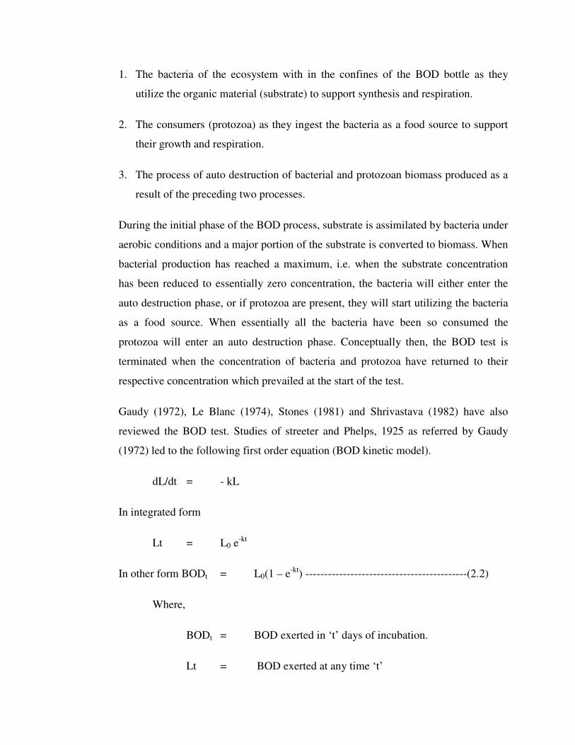
1. The bacteria of the ecosystem with in the confines of the BOD bottle as they

utilize the organic material (substrate) to support synthesis and respiration.

2. The consumers (protozoa) as they ingest the bacteria as a food source to support

their growth and respiration.

3. The process of auto destruction of bacterial and protozoan biomass produced as a

result of the preceding two processes.

During the initial phase of the BOD process, substrate is assimilated by bacteria under

aerobic conditions and a major portion of the substrate is converted to biomass. When

bacterial production has reached a maximum, i.e. when the substrate concentration

has been reduced to essentially zero concentration, the bacteria will either enter the

auto destruction phase, or if protozoa are present, they will start utilizing the bacteria

as a food source. When essentially all the bacteria have been so consumed the

protozoa will enter an auto destruction phase. Conceptually then, the BOD test is

terminated when the concentration of bacteria and protozoa have returned to their

respective concentration which prevailed at the start of the test.

Gaudy (1972), Le Blanc (1974), Stones (1981) and Shrivastava (1982) have also

reviewed the BOD test. Studies of streeter and Phelps, 1925 as referred by Gaudy

(1972) led to the following first order equation (BOD kinetic model).

dL/dt = - kL

In integrated form

Lt = L0 e-kt

In other form BODt = L0(1 – e-kt) -------------------------------------------(2.2)

Where,

BODt = BOD exerted in ‘t’ days of incubation.

Lt = BOD exerted at any time ‘t’

L0 = Oxygen demand yet to be exerted at t=0 i.e. ultimate

BOD.

k = BOD reaction rate constant and its units are time-1.

t = Time of incubation.

Analysis of the above first order equation indicates two variables, rate constant k and

ultimate BOD, L0 are dependent on each other. If the rate of biochemical oxidation is

very high, the value BOD5 is essentially equal to the ultimate BOD. (Ramallho,

1983). Maity and Ganguly (2002) observed that experimental ‘k’ value is always

greater than the theoretical ‘k’ value by 18% and 24%, when the sample is tested at

20oC and at 27oC respectively. Shrivastava (2000) studied the effect of sewage and

indigenous seed on BOD exertion and found that with indigenous seed the BOD

values are observed more and kinetic study revealed that with indigenous seed the

ultimate BOD is more and value of rate constant is higher in both first order and

second order equations with sewage seed. Typical values of k and L0 are listed in

table 2.1 (Peavy, 1985)

Table: 2.1 Typical values of k & L0 for various waters.

Water Type K (Day-1) L0 (mg/l)

Tap water <0.1 0 – 1

Surface water 0.1 – 0.23 1 – 30

Weak municipal waste water 0.35 150

Strong municipal waste water 0.40 250

Treated effluent 0.12 – 0.23 10 – 30

Reddy reported that kinetics of BOD exertion pattern involves the following:

(i) Mathematical modeling of the oxygen demand pattern of the sample being

incubated

(ii) Using such a mathematical model for extrapolating the results obtain and

finding out the rate constant and ultimate BOD.

There are different methods of estimation of kinetic parameters k & L0. Before an

estimate of k & L0 can be made a set of progressive long-term (10 to 15 days) BOD

data must be obtained (Merske et.al, 1972). The work of Berthouex et.al, (1971)

showed that the estimation of BOD constants is most accurate when longer BOD test

data, with the addition of nitrification inhibitors, are considered. To calculate k & L0

from given series of BOD measurements is fundamentally a curve-fitting problem.

Reed et.al, (1931) published a paper on the statistical treatment of velocity data, that

is recognized as the most comprehensive and accurate approach to the estimation of

the velocity constants of the first order model for the BOD kinetics. However as this

method requires laborious calculations and therefore one is discouraged from

estimating k & L0 (Merske et.al, 1972).

Fair (1936) proposed the log-difference method for the solution of the BOD equation,

but was difficult to be solved. The method involved the plotting of daily difference

between the BOD values versus time. Thomas (1937) developed the slope method

(graphical) and for many years this was the most used method for computing the

kinetics parameters. Thomas (1950) proposed a simple graphical approximation for

evaluation of the constants of BOD curve, which is based on similarity function.

Moor et.al, (1950) developed the method of moments, which became the most used

technique of solving BOD kinetics parameters. The method involves constructing of

Moore’ s diagram of ∑BOD/L0 versus k and ∑BOD/∑BOD.t versus k for the

particular number of days for which the BOD data is available. Remo Navone (1960)

published a new method for calculating BOD constant for sewage. This method

simplified the calculation of these parameters. The least squares method involves

fitting a curve through a set of data points, so that sum of the squares of the difference

between the observed value and the value of the fitted curve must be minimum

(Metcalf & Eddy, 2003). Fujimoto (1961), suggested an arithmetic plot between

BODt+1 versus BODt, and the intersection of this plot with line of slope 1 corresponds

to the ultimate BOD(L0).

Gurjar (1994) suggested a new simple method to determine first stage BOD constants

(k & L0). Guillermo Cutrera et.al, (1999), compared the three methods (non linear

fitting, linear fitting & Thomas method) for estimation of k & L0 and found that non-

linear method of least squares results in smallest error.

Rai (2000) suggested a simplified method for determination of BOD constants. He

suggested the iteration method for estimation of k & L0. Riefler and Smets. (2003)

compared the type curve method with least square error method to estimate biofilm

kinetic parameters & observed that more accurate and precise estimates were

obtained with least square error method.

CHAPTER: 3

Materials And Methods

3.1 Introduction

In the study, serial BOD testing for BOD kinetics was conducted on six different

types of samples (treated municipal sewage, treated distillery effluent, treated textile

effluent, treated dairy effluent, water sample collected from river Satluj near village

Sangowal and water sample collected from river East Bein, a tributary to river satluj,

at Malsian village). The experiments were conducted in triplicate. Samples of the

river Satluj and the river East Bein were analyzed for BOD kinetics, during June to

Sept. 2003, and the samples from other four sources were studied during Oct. to Dec.

2003. Results of the serial BOD tests were used in evaluating different methods used

for estimating the BOD kinetics parameters (k and L0). Evaluation of the methods

was done through calculating and comparing the sum of the absolute differences

between the observed BOD and exerted BOD.

3.2 Sampling

Grab samples were collected from each of the six sources, once a month for three

months. In case of river water samples the sampling was done for four months. The

collected samples were brought to the laboratory in an insulated box. For avoiding

deterioration of the samples during transportation, the box containing the sample was

filled with ice cubes. In the laboratory the samples were retained in a refrigerator and

used in the BOD kinetics experimentation within 2 days time from the day of

collection.

3.2 serial BOD testing

For estimating the BOD kinetics parameters, k and Lo, serial BOD measurements for

the first 7 days were made for the prepared samples incubated at 20C. That is, BOD1,

BOD2, ---and BOD7 were measured for the sample in question. BOD bottle method

described in Standard Method, 1995 Method No. 5210B, was used for these

measurements.

24 BOD bottles were used in the experiment for facilitating daily DO measurement in

triplicate, as a part of the BOD test. Dilution factor approximating to COD/6 was used

for diluting the sample. Aerated distilled water containing 1 ml per liter each of ferric

chloride solution, magnesium sulphate solution, phosphate buffer solution and

calcium chloride solution was used as dilution water. These solutions and the

solutions used in COD measurements and DO measurements were prepared as per the

procedure and strengths indicated in the Standard Method, 1995 under the

corresponding methods. In case of industrial effluents 1 ml per liter of acclimatized

seed was also added to this dilution water. Supernatant of settled secondary sludge

from the ETP of the same industry was used as acclimatized seed.

The sample in question was first tested for COD using the method given in Standard

Method, 1995 Method No. 5220-C. On the basis of the COD dilution factor was

found out and used in the preparation of the diluted sample for serial BOD test. 12

liter of diluted sample was prepared and after sufficient aeration the sample was

transfered into the 24 BOD bottles. While analyzing 3 of the bottles for initial DO,

rest of the bottles were incubated in a BOD incubator at 20oC for 7 days. Every day 3

of the incubated bottles were taken out and tested for DO while using the technique

given in Standard Method, 1995 Method No. 4500-O.C. BOD of the sample was

estimated by using the following expressions:

BODt at 20oC = DF [(DOis-DOfs)-(DOib-Dofb)(1-1/DF)]-----------------(3.1)

Where,

BODt = BOD exerted in ‘t’ days of incubation.

DOis = DO of the diluted sample immediately after preparation,

mg/l.

DOfs = DO of the diluted sample at particular day of

incubation, mg/l.

DOib = DO of seed control before incubation, mg/l.

DOfb = DO of seed control after incubation, mg/l.

DF = Dilution factor.

3.4 Estimation of BOD kinetic Parameters: Using the results obtained from serial

BOD test, BOD and time were plotted and through extending the smooth curve

passing through the data points to the x-axis time lag involved in the test was

estimated (fig. 3.1). On the basis of the lag obtained the first order BOD kinetic

equation was corrected as below:

BODt = L0 (1-e-k . (t-lag time))

The corrected kinetics equation was used in all the calculations, except in case of

method of moments, the original BOD kinetic equation and nomograph for n = 7days

was used. Using the results obtained from the serial BOD tests, BOD kinetics

parameters (k and L0) were estimated by the following six different methods, which

are commonly used:

(i) Method of Moments (Ramallho, 1983)

(ii) Least Squares Method (Metcalf Eddy, 2003)

(iii) Thomas Graphical Method (McGhee, 1991)

(iv) Daily Difference Method (Ramallho, 1983)

(v) Iteration Method (Rai, R.K., 2000)

(vi) Fujimoto Method (Metcalf Eddy, 2003)

Fig. 3.1: Lag of 0.9 day in Textile sample-III

0

500

1000

1500

2000

2500

3000

3500

4000

0 1 2 3 4 5 6 7 8

Time(days)

BO

D(m

g/l)

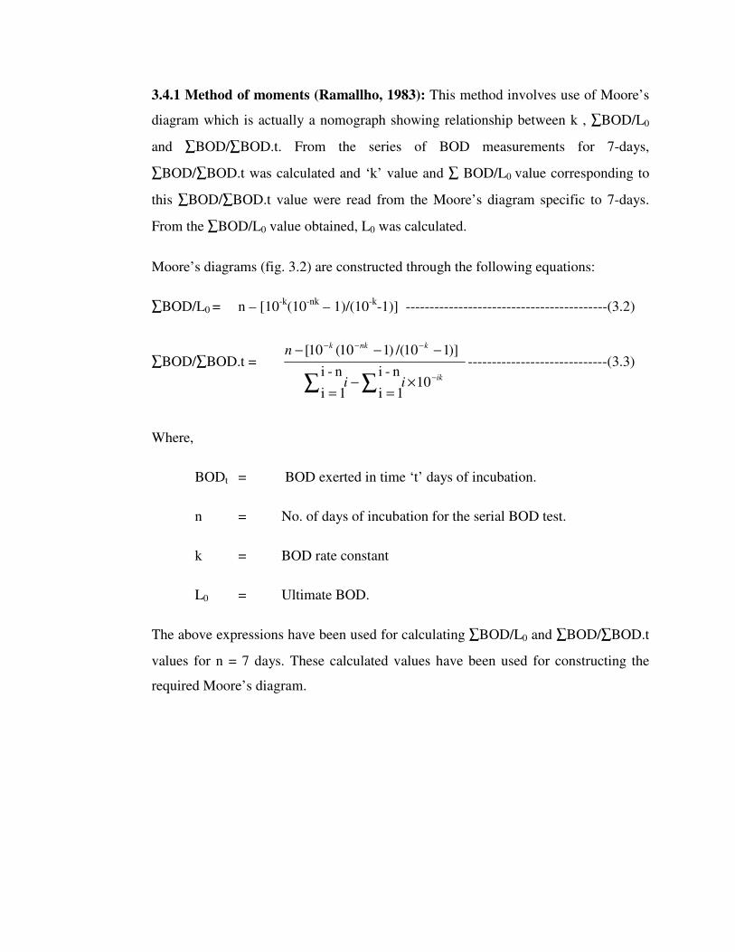
3.4.1 Method of moments (Ramallho, 1983): This method involves use of Moore’ s

diagram which is actually a nomograph showing relationship between k , ∑BOD/L0

and ∑BOD/∑BOD.t. From the series of BOD measurements for 7-days,

∑BOD/∑BOD.t was calculated and ‘k’ value and ∑ BOD/L0 value corresponding to

this ∑BOD/∑BOD.t value were read from the Moore’ s diagram specific to 7-days.

From the ∑BOD/L0 value obtained, L0 was calculated.

Moore’ s diagrams (fig. 3.2) are constructed through the following equations:

∑BOD/L0 = n – [10-k(10-nk – 1)/(10-k-1)] ------------------------------------------(3.2)

∑BOD/∑BOD.t = ik

knkk

ii

n

−

−−−

×=

−=

−−−

∑∑ 101i

n-i1i

n-i)]110/()110(10[

-----------------------------(3.3)

Where,

BODt = BOD exerted in time ‘t’ days of incubation.

n = No. of days of incubation for the serial BOD test.

k = BOD rate constant

L0 = Ultimate BOD.

The above expressions have been used for calculating ∑BOD/L0 and ∑BOD/∑BOD.t

values for n = 7 days. These calculated values have been used for constructing the

required Moore’ s diagram.

Fig. 3.2 : Moore’s diagram for n=7 days

0

1

2

3

4

5

6

7

8

0 0.4 0.8 1.2 1.6 2

k(day-1)

BO

D/L

0

0.198

0.218

0.238

0.258

BO

D/B

OD

.t

BOD/LoBOD/BOD.t

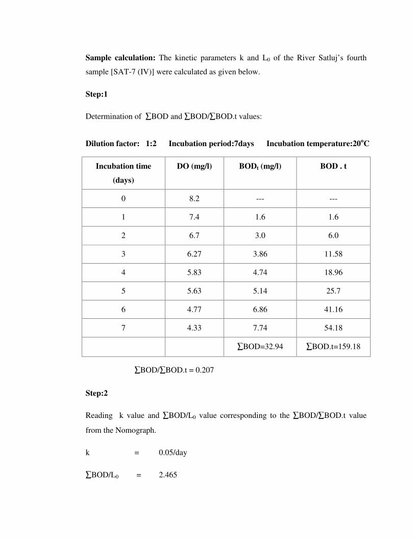
Sample calculation: The kinetic parameters k and L0 of the River Satluj’ s fourth

sample [SAT-7 (IV)] were calculated as given below.

Step:1

Determination of ∑BOD and ∑BOD/∑BOD.t values:

Dilution factor: 1:2 Incubation period:7days Incubation temperature:20oC

Incubation time

(days)

DO (mg/l) BODt (mg/l) BOD . t

0 8.2 --- ---

1 7.4 1.6 1.6

2 6.7 3.0 6.0

3 6.27 3.86 11.58

4 5.83 4.74 18.96

5 5.63 5.14 25.7

6 4.77 6.86 41.16

7 4.33 7.74 54.18

∑BOD=32.94 ∑BOD.t=159.18

∑BOD/∑BOD.t = 0.207

Step:2

Reading k value and ∑BOD/L0 value corresponding to the ∑BOD/∑BOD.t value

from the Nomograph.

k = 0.05/day

∑BOD/L0 = 2.465

Step 3:

Estimation of L0 value

L0 = ∑BOD/(∑BOD/L0) = 2.465/32.94 = 13.36 mg/l

3.4.2 Least Squares Method (Metcalf Eddy 2003): According to first order kinetics

dL/dt = - kLt

where,

Lt = L0 - yt

yt = BODt

dy/dt = k (L0 – yt)

dy/dt = kL0 – kyt

This is a linear equation. Through use of least squares method k & L0 values in the

above linear equation can be found out. In the calculations the following equation are

used:-

Sxx = n ∑yt2 – (∑ y)2 -----------------------------------------------(3.4)

Sxy = n∑yt(dy/dt) – (∑yt) (∑dy/dt) ---------------------------------(3.5)

Slope (-k) = Sxy / Sxx ---------------------------------------------------------(3.6)

Intercept (kL0) =∑ (dy/dt)/n + k∑(yt)/n -----------------------------------------------(3.7)

L0 = Intercept/(-slope) ----------------------------------------------(3.8)

Sample calculation:

The kinetic parameters k & L0 of the river Satluj’ s fourth sample [SAT-7(IV)] were

estimated as follows:

Step 1:

Constructing the following table:

Time yt dy/dt = (yt+1 – yt-1)/2¨W yt2 yt.dy/dt

1 1.60 1.50 2.56 2.40

2 3.00 1.13 9.00 27.0

3 3.86 0.87 14.90 3.34

4 4.74 0.63 22.47 4.88

5 5.14 1.07 26.42 5.50

6 6.86 1.30 47.06 8.92

7 7.74*

Sums 25.20 6.50 122.42 26.55

* Value not included in total and n = 6 is used.

Step 2:

Substituted the value computed in Step 1 in eq. (3.4) and (3.5).

Sxx = 99.48

Sxy = - 4.5

Step 3:

Calculated k and L0 by using eq. (3.6), (3.7) and (3.8).

k = 0.045/day

L0 = 28.17 mg/l

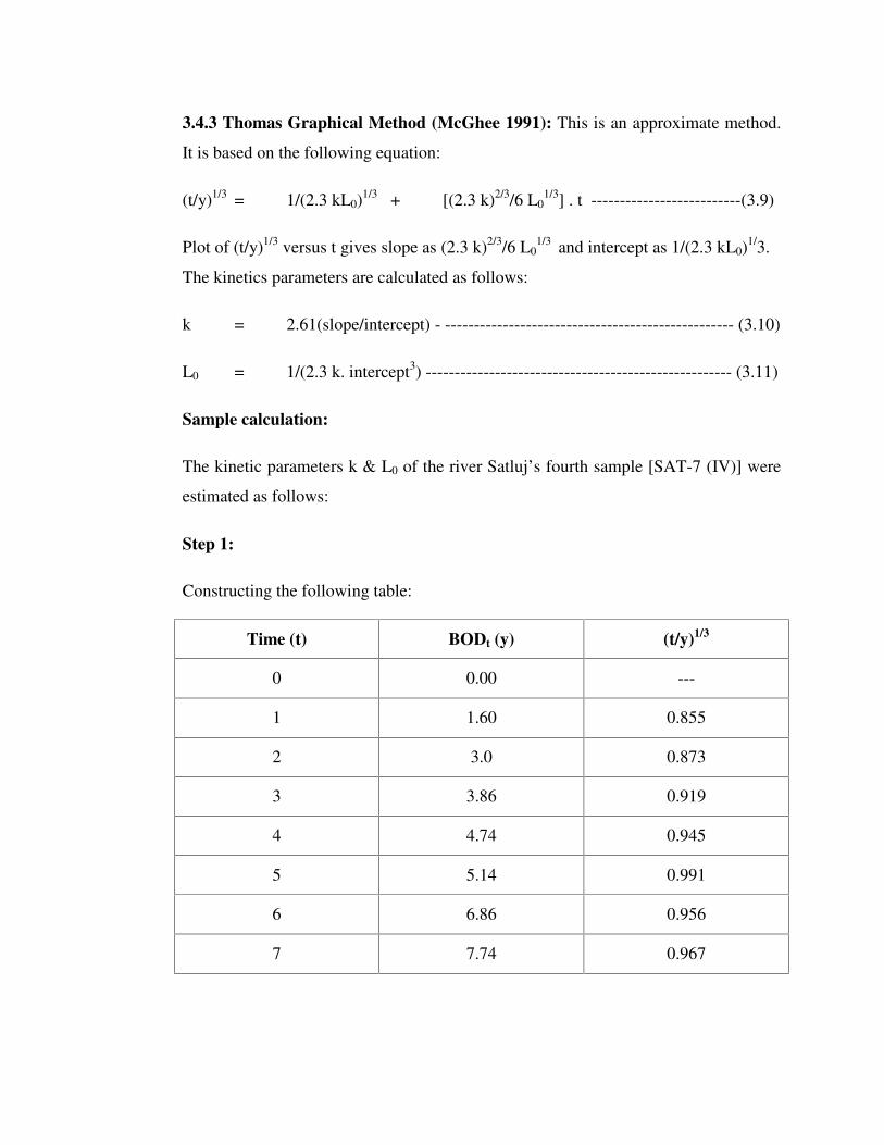
3.4.3 Thomas Graphical Method (McGhee 1991): This is an approximate method.

It is based on the following equation:

(t/y)1/3 = 1/(2.3 kL0)1/3 + [(2.3 k)2/3/6 L01/3] . t --------------------------(3.9)

Plot of (t/y)1/3 versus t gives slope as (2.3 k)2/3/6 L01/3 and intercept as 1/(2.3 kL0)1/3.

The kinetics parameters are calculated as follows:

k = 2.61(slope/intercept) - -------------------------------------------------- (3.10)

L0 = 1/(2.3 k. intercept3) ----------------------------------------------------- (3.11)

Sample calculation:

The kinetic parameters k & L0 of the river Satluj’ s fourth sample [SAT-7 (IV)] were


Step 1:


Time (t) BODt (y) (t/y)1/3

0 0.00 ---

1 1.60 0.855

2 3.0 0.873

3 3.86 0.919

4 4.74 0.945

5 5.14 0.991

6 6.86 0.956

7 7.74 0.967

Step 2:

Plotted (t/y)1/3 versus ‘t’ (fig. 3.3) and found slope and intercept as given below:

Slope = 0.0205

Intercept = 0.8474

Step 3: From equation (3.10) and (3.11), obtained k and L0:

k = 0.063/day

L0 = 11.34 mg/l

Fig. 3.3: Thomas’ Method for SAT-7(IV)

y = 0.0205x + 0.8474

0.8

0.82

0.84

0.86

0.88

0.9

0.92

0.94

0.96

0.98

1

0 1 2 3 4 5 6 7 8

Days

(t/y

)1/3

3.4.4 Daily Difference Method (Ramallho,1983):

According to first order equation:

y = L0 (1- 10-kt)

dy/dt = L0 (-10-kt )(ln10)(-k)

log(dy/dt) = log(2.303 kL0) – kt -----------------------------(3.12)

Plotting log (dy/dt) versus time (midinterval value of ‘t’ ) gives slope as –k and

intercept as log(2.303 kL0). Ultimate BOD (L0) can then be obtained by the following

equation:

L0 = 10(intercept) / 2.303 (k). -----------------------------(3.13)

Sample calculation:



Step 1:


Time (t) y (mg/l) dy/dt log dy/dt Midinterval value

of t

0 0 --- --- ---

1 1.60 1.60 0.204 0.50

2 3.00 1.40 0.146 1.50

3 3.86 0.86 - 0.066 2.50

4 4.74 0.88 - 1.056 3.50

5 5.14 0.40 - 0.398 4.50

6 6.86 1.72 0.236 5.50

7 7.74 0.88 - 1.056 6.50

Step 2:

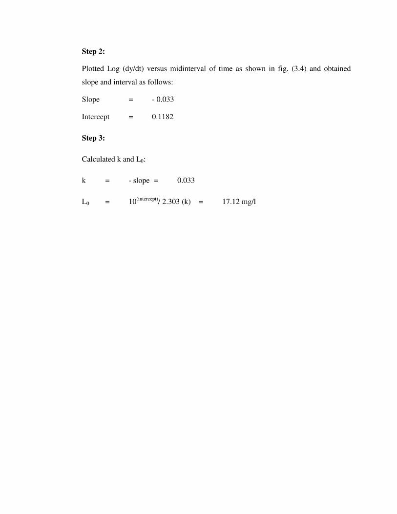
Plotted Log (dy/dt) versus midinterval of time as shown in fig. (3.4) and obtained

slope and interval as follows:

Slope = - 0.033

Intercept = 0.1182

Step 3:

Calculated k and L0:

k = - slope = 0.033

L0 = 10(intercept)/ 2.303 (k) = 17.12 mg/l

Fig. 3.4: Daily difference method for Sat-7(IV)

y = -0.0333x + 0.1182

-0.5

-0.4

-0.3

-0.2

-0.1

0

0.1

0.2

0.3

0 1 2 3 4 5 6 7

Time (Days)

log

(dy/

dt)

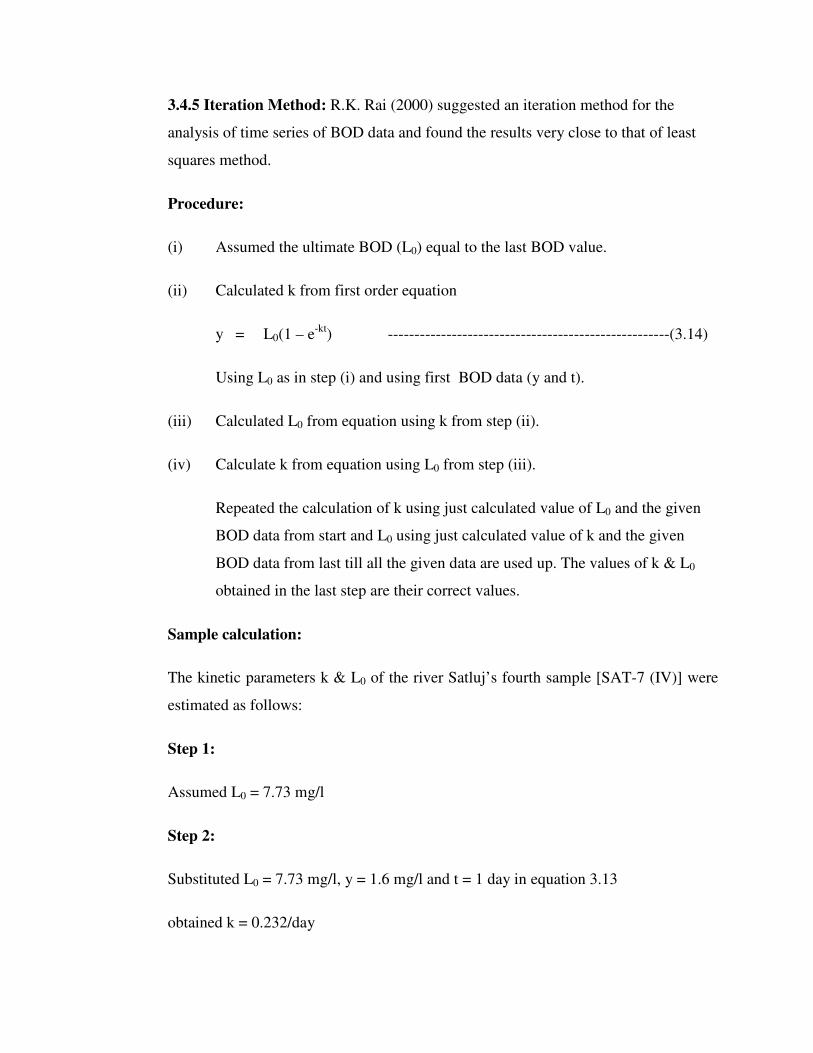
3.4.5 Iteration Method: R.K. Rai (2000) suggested an iteration method for the

analysis of time series of BOD data and found the results very close to that of least

squares method.

Procedure:

(i) Assumed the ultimate BOD (L0) equal to the last BOD value.

(ii) Calculated k from first order equation

y = L0(1 – e-kt) -----------------------------------------------------(3.14)

Using L0 as in step (i) and using first BOD data (y and t).

(iii) Calculated L0 from equation using k from step (ii).

(iv) Calculate k from equation using L0 from step (iii).

Repeated the calculation of k using just calculated value of L0 and the given

BOD data from start and L0 using just calculated value of k and the given

BOD data from last till all the given data are used up. The values of k & L0

obtained in the last step are their correct values.

Sample calculation:



Step 1:

Assumed L0 = 7.73 mg/l

Step 2:

Substituted L0 = 7.73 mg/l, y = 1.6 mg/l and t = 1 day in equation 3.13

obtained k = 0.232/day

Step 3:

Substituted k = 0. 232/day, y = 7.73 mg/l and t = 7 in equation 3.13

obtained L0 = 9.628 mg/l

Step 4:

Substituted L0 = 9.628 mg/l, y = 3.0 mg/l and t = 2 days in equation 3.13


Step 5:

Substituted k =0.187/day, y = 6.87 mg/l and t = 6 days in equation 3.13

obtained L0 = 10.19 mg/l

Step 6:

Substituted L0 = 10.19 mg/l, y = 3.87 mg/l and t = 3 days in equation 3.13

obtained k = 0.159/day.

Step 7:

Substituted k = 0.159/day, y = 5.13 and t = days in equation 3.13

obtained L0 = 9.35mg/l

Step 8:

Substituted L0 = 9.35mg/l, y = 4.73mg/l and t = 4 days in equation 3.13


Step 9:

The values of BOD constants are, therefore

L0 = 9.35mg/l and k = 0.176/day

3.4.6 Fujimoto method (Metcalf Eddy 2003): Using this method an arithmetic plot

was prepared of BODt+1 versus BODt. The value at the intersection of the plot with a

line of slope 1 corresponds to the ultimate BOD. The rate constant k was determined

from the following equation:

BODt = L0 (1-e-kt)--------------------------------------------- (3.15)

Where,

BODt = BOD exerted in time ‘t’ days of incubation.

L0 = Ultimate BOD

t = time (days)

Sample calculation:



Step 1:

Prepared and arithmetic plot of BODt+1 versus BODt (fig. 3.5) using the following

table:

Sr.No. 1 2 3 4 5 6

BODt

(mg/l)

1.60 3.00 3.86 4.74 5.14 6.86

BODt+1

(mg/l)

3.00 3.86 4.74 5.14 6.86 7.74

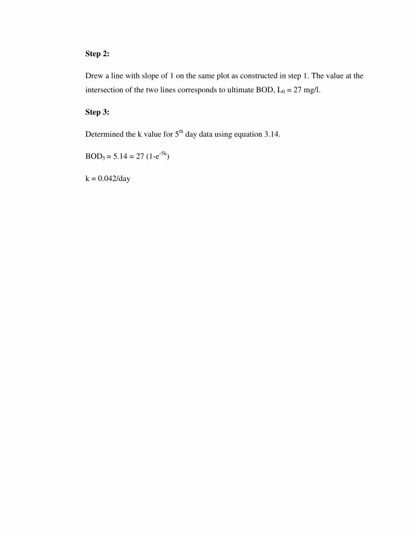
Step 2:

Drew a line with slope of 1 on the same plot as constructed in step 1. The value at the

intersection of the two lines corresponds to ultimate BOD, L0 = 27 mg/l.

Step 3:

Determined the k value for 5th day data using equation 3.14.

BOD5 = 5.14 = 27 (1-e-5k)

k = 0.042/day

Fig. 5: Fujimoto Method For SAT7-IV

0

5

10

15

20

25

30

35

40

45

50

0 5 10 15 20 25 30 35 40 45 50

BODt

BO

Dt+

1

3.5 Comparison of different methods of estimation: The methods are compared by

plotting observed BOD values and expected BOD values during 7 days for six

different methods against time. Evaluation of different methods was done by

calculating the sum of absolute differences between the observed and expected BOD

values as follows:

D = �� (oi – ei) /ei

Where, oi and ei are the observed BOD and expected BOD values calculated by using

estimated kinetic parameters by each method.

CHAPTER: 4

Results and Discussion

4.1 Introduction

This chapter includes, the results obtained from the serial BOD tests, the BOD kinetic

parameters estimation by different methods and the evaluation of different methods of

BOD kinetic parameters estimation through sum of the absolute differences between

the observed and expected BOD values during 7 days. Further, the results obtained

are discussed to indicate how far the BOD kinetic parameters estimation methods are

reliable and which of the methods has proved most appropriate in the present study.

4.2 Results

Results obtained from the serial BOD tests for 7 days of incubation and from the

COD tests on the following six different types of samples are presented in the tables

4.1 to 4.6.

1) Satluj river water sample

2) East Bein river water sample

3) Treated Municipal sewage sample

4) Treated Distillery effluent

5) Treated Dairy effluent

6) Treated Textile effluent

Table: 4.1 BOD results of River Satluj (SAT-7).

BODt(mg/l) Days

Sample I Sample II Sample III Sample IV

1 1.02 0.20 0.77 1.60

2 2.70 0.74 1.80 3.00

3 3.80 2.54 2.43 3.86

4 4.00 2.94 2.83 4.74

5 4.42 3.54 3.48 5.14

6 4.80 4.20 3.70 6.86

7 6.56 4.60 4.17 7.74

COD

(mg/l)

16.00 21.00 9.00 25.00

Table: 4.2 BOD results of East Bein river (EB-4).

BODt(mg/l) Days


1 6.60 2.60 5.50 10.00

2 15.20 13.30 23.25 21.50

3 28.20 23.60 31.75 51.50

4 35.00 28.60 38.25 61.50

5 44.60 33.30 49.25 71.50

6 49.33 37.00 57.50 88.50

7 62.00 39.30 62.50 95.00

COD

(mg/l)

176.00 115.00 350.00 727.00

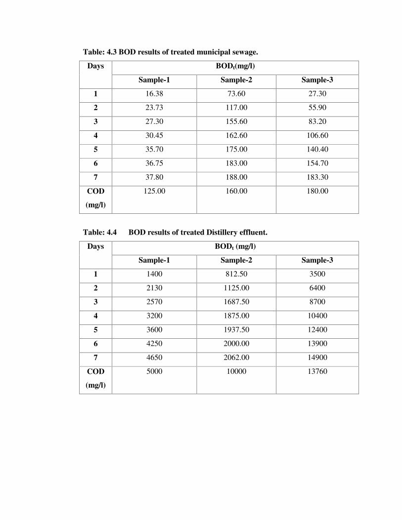
Table: 4.3 BOD results of treated municipal sewage.

BODt(mg/l) Days

Sample-1 Sample-2 Sample-3

1 16.38 73.60 27.30

2 23.73 117.00 55.90

3 27.30 155.60 83.20

4 30.45 162.60 106.60

5 35.70 175.00 140.40

6 36.75 183.00 154.70

7 37.80 188.00 183.30

COD

(mg/l)

125.00 160.00 180.00

Table: 4.4 BOD results of treated Distillery effluent.

BODt (mg/l) Days


1 1400 812.50 3500

2 2130 1125.00 6400

3 2570 1687.50 8700

4 3200 1875.00 10400

5 3600 1937.50 12400

6 4250 2000.00 13900

7 4650 2062.00 14900

COD

(mg/l)

5000 10000 13760

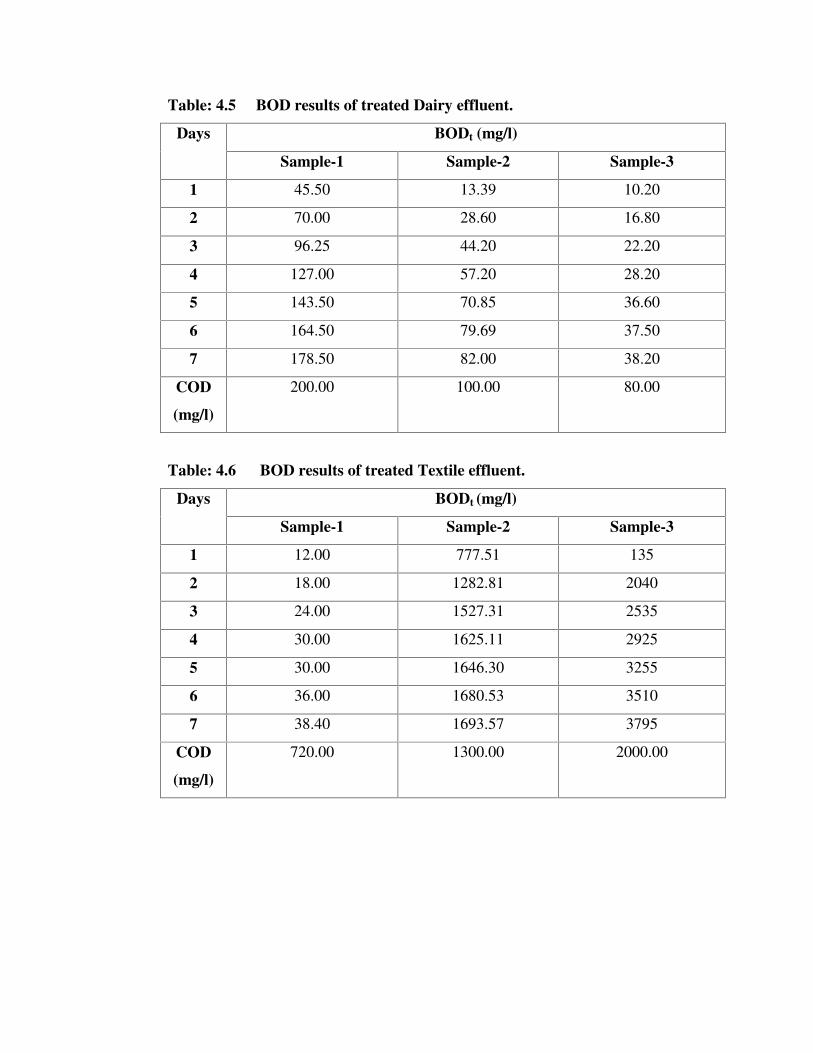
Table: 4.5 BOD results of treated Dairy effluent.

BODt (mg/l) Days


1 45.50 13.39 10.20

2 70.00 28.60 16.80

3 96.25 44.20 22.20

4 127.00 57.20 28.20

5 143.50 70.85 36.60

6 164.50 79.69 37.50

7 178.50 82.00 38.20

COD

(mg/l)

200.00 100.00 80.00

Table: 4.6 BOD results of treated Textile effluent.

BODt (mg/l) Days


1 12.00 777.51 135

2 18.00 1282.81 2040

3 24.00 1527.31 2535

4 30.00 1625.11 2925

5 30.00 1646.30 3255

6 36.00 1680.53 3510

7 38.40 1693.57 3795

COD

(mg/l)

720.00 1300.00 2000.00

The results obtained, from serial BOD tests were checked for involvement of any lag

phase and wherever there is a lag phase its duration was measured. Duration of lag,

obtained in serial BOD tests is given in table 4.7.

Table: 4.7 Duration of lag observed in serial BOD test.

Lag Values (day)

Samples Sample I Sample II Sample III Sample IV

River Satluj

(SAT-7)

0.5 0.85 0.35 Nil

East Bein

River (EB-4)

Nil 0.80 0.75 Nil

Treated

Municipal

Sewage

Nil Nil Nil ----

Treated

Distillery

Effluent

Nil Nil Nil ----

Treated Dairy

Effluent

Nil 0.20 Nil ----

Treated Textile

Effluent

Nil Nil 0.9 ----

BOD kinetics parameters (k and L0) calculated from the serial BOD test results using

the following six different methods of BOD kinetic parameters estimation, for each of

the samples on which serial BOD tests were conducted, are presented in the tables 4.8

to 4.13:

1) Method of moments

2) Least squares method

3) Thomas method

4) Daily difference method

5) Iteration method

6) Fujimoto method

COD values and BOD5 /COD values at 20oC are included in these tables.

Table: 4.8 BOD Kinetic Parameters Values for the Satluj River water (SAT-7)

* ‘k’ values are to base 10.

Kinetic Parameters Values


Methods

K L0 K L0 K L0 K L0

Moments* 0.067 9.27 0.00002 14430 0.067 6.51 0.05 13.36

Least squares 0.221 7.36 0.037 21.83 0.195 5.54 0.045 28.17

Thomas* 0.146 6.39 0.049 9.44 0.421 2.45 0.063 11.34

Daily Difference* 0.051 9.4 0.027 18.46 0.082 5.38 0.033 17.12

Iteration 0.414 5.25 0.160 7.42 0.248 4.75 0.176 9.35

Fujimoto 0.172 8.2 0.170 7.00 0.256 5.00 0.042 27.0

COD (mg/l) 16.0 21.0 9.0 25.0

BOD5/COD 0.276 0.169 0.395 0.206

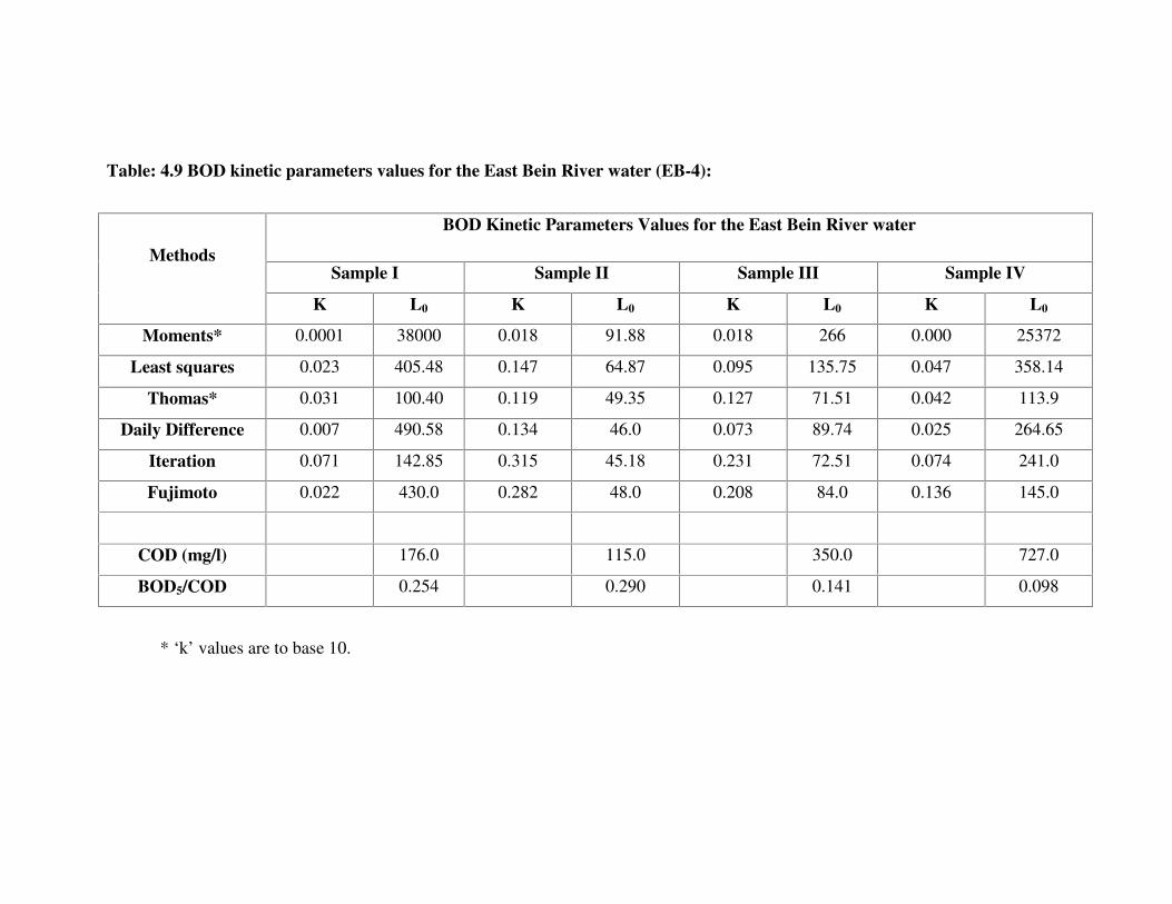
Table: 4.9 BOD kinetic parameters values for the East Bein River water (EB-4):


BOD Kinetic Parameters Values for the East Bein River water


Methods

K L0 K L0 K L0 K L0

Moments* 0.0001 38000 0.018 91.88 0.018 266 0.000 25372

Least squares 0.023 405.48 0.147 64.87 0.095 135.75 0.047 358.14

Thomas* 0.031 100.40 0.119 49.35 0.127 71.51 0.042 113.9

Daily Difference 0.007 490.58 0.134 46.0 0.073 89.74 0.025 264.65

Iteration 0.071 142.85 0.315 45.18 0.231 72.51 0.074 241.0

Fujimoto 0.022 430.0 0.282 48.0 0.208 84.0 0.136 145.0

COD (mg/l) 176.0 115.0 350.0 727.0

BOD5/COD 0.254 0.290 0.141 0.098

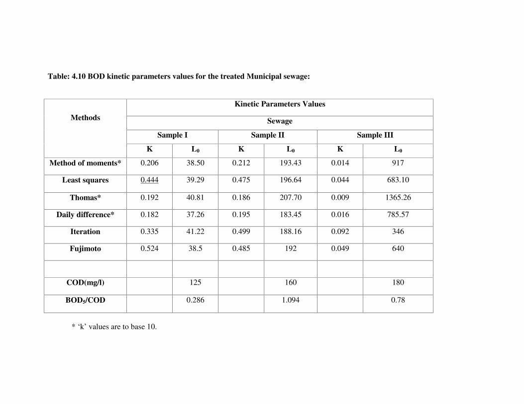
Table: 4.10 BOD kinetic parameters values for the treated Municipal sewage:


Sewage

Sample I Sample II Sample III

Methods

K L0 K L0 K L0

Method of moments* 0.206 38.50 0.212 193.43 0.014 917

Least squares 0.444 39.29 0.475 196.64 0.044 683.10

Thomas* 0.192 40.81 0.186 207.70 0.009 1365.26

Daily difference* 0.182 37.26 0.195 183.45 0.016 785.57

Iteration 0.335 41.22 0.499 188.16 0.092 346

Fujimoto 0.524 38.5 0.485 192 0.049 640

COD(mg/l) 125 160 180

BOD5/COD 0.286 1.094 0.78


Table: 4.11 BOD kinetic parameters values for the treated Distillery Effluent:


Distellery


Methods

K L0 K L0 K L0

Method of moments* 0.1 5578.30 0.192 2183.13 0.078 21384.83

Least squares 0.157 6839.22 0.412 2230.28 0.175 21264.28

Thomas* 0.117 5200.84 0.173 2327 0.077 21239.71


Iteration 0.227 5356.47 0.521 2141.98 0.196 19166.45

Fujimoto 0.082 10700 0.447 2170 0.172 21500.00

COD(mg/l) 5000 10000 13760

BOD5/COD 0.72 0.194 0.901


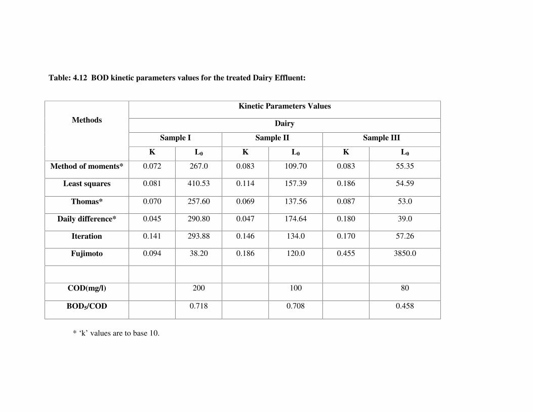
Table: 4.12 BOD kinetic parameters values for the treated Dairy Effluent:


Dairy


Methods

K L0 K L0 K L0


Least squares 0.081 410.53 0.114 157.39 0.186 54.59

Thomas* 0.070 257.60 0.069 137.56 0.087 53.0


Iteration 0.141 293.88 0.146 134.0 0.170 57.26

Fujimoto 0.094 38.20 0.186 120.0 0.455 3850.0

COD(mg/l) 200 100 80

BOD5/COD 0.718 0.708 0.458


Table: 4.13 BOD kinetic parameters values for the treated Textile Effluent:


Textile


Methods

K L0 K L0 K L0


Least squares 0.228 47.81 0.703 1731.0 0.259 4706.95

Thomas* 0.125 43.41 0.231 1916.46 0.179 4232


Iteration 0.329 41.00 0.83 1686.36 0.528 3631.11

Fujimoto 0.151 56.50 0.096 4300.0 0.455 3850.0

COD(mg/l) 720 1300 2000

BOD5/COD 0.042 1.266 1.628


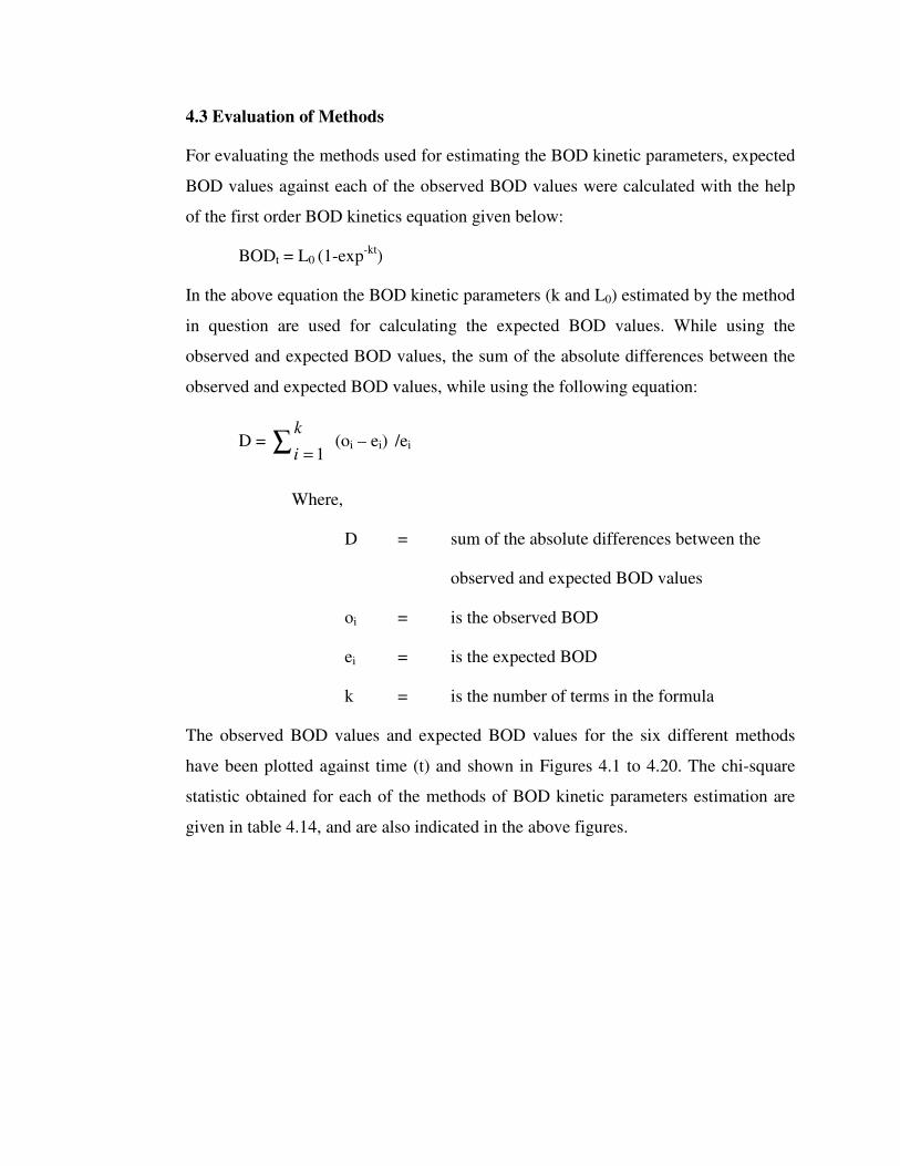
4.3 Evaluation of Methods

For evaluating the methods used for estimating the BOD kinetic parameters, expected

BOD values against each of the observed BOD values were calculated with the help

of the first order BOD kinetics equation given below:

BODt = L0 (1-exp-kt)

In the above equation the BOD kinetic parameters (k and L0) estimated by the method

in question are used for calculating the expected BOD values. While using the

observed and expected BOD values, the sum of the absolute differences between the

observed and expected BOD values, while using the following equation:

D = ∑ = 1i

k (oi – ei) /ei

Where,

D = sum of the absolute differences between the

observed and expected BOD values

oi = is the observed BOD

ei = is the expected BOD

k = is the number of terms in the formula

The observed BOD values and expected BOD values for the six different methods

have been plotted against time (t) and shown in Figures 4.1 to 4.20. The chi-square

statistic obtained for each of the methods of BOD kinetic parameters estimation are

given in table 4.14, and are also indicated in the above figures.

Table: 4.14 Sum of absolute differences of observed and expected BOD values:

Methods

Sample

Moments Least Squares

Thomas Daily difference

Iteration Fujimoto

SAT-7 (I) 0.83 1.13 0.62 2.98 0.64 1.59

SAT-7 (II) 0.15 0.18 0.37 0.17 0.30 2.59

SAT-7 (III) 0.37 0.52 2.33 0.93 0.47 0.19

SAT-7 (IV) 0.44 0.78 0.41 0.93 0.50 1.43

EB-4 (I) 0.55 0.63 2.50 0.99 0.72 0.62

EB-4 (II) 6.07 1.34 0.17 0.19 0.21 0.12

EB-4 (III) 0.75 1.72 0.45 1.27 1.05 0.66

EB-4 (IV) 0.99 0.92 3.70 1.24 0.94 1.07

Sewage-I 0.32 0.34 0.40 0.67 0.73 0.31

Sewage-II 0.16 0.19 0.26 0.60 0.15 0.11

Sewage-III 0.22 0.22 0.14 0.16 0.41 0.36

Distillery-I 0.49 0.64 0.47 0.96 0.57 1.18

Distillery-II 0.28 0.33 0.38 0.59 0.32 0.27

Distillery-III 0.15 0.09 0.08 0.07 0.20 0.10

Dairy - I 0.38 0.86 0.32 2.03 0.35 0.52

Dairy – II 0.71 0.25 0.70 0.35 0.31 0.56

Dairy – III 0.38 0.36 0.36 0.93 0.37 0.95

Textile-I 0.41 0.54 0.42 0.82 0.42 1.09

Textile-II 0.15 0.18 0.37 0.17 0.30 2.59

Textile-III 1.47 1.37 0.74 1.74 0.73 0.69

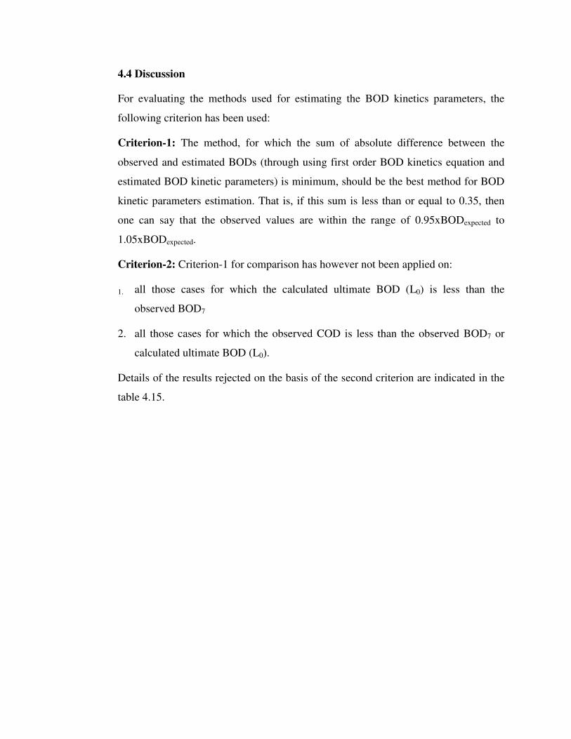
4.4 Discussion

For evaluating the methods used for estimating the BOD kinetics parameters, the

following criterion has been used:

Criterion-1: The method, for which the sum of absolute difference between the

observed and estimated BODs (through using first order BOD kinetics equation and

estimated BOD kinetic parameters) is minimum, should be the best method for BOD

kinetic parameters estimation. That is, if this sum is less than or equal to 0.35, then

one can say that the observed values are within the range of 0.95xBODexpected to

1.05xBODexpected.

Criterion-2: Criterion-1 for comparison has however not been applied on:

1. all those cases for which the calculated ultimate BOD (L0) is less than the

observed BOD7

2. all those cases for which the observed COD is less than the observed BOD7 or

calculated ultimate BOD (L0).

Details of the results rejected on the basis of the second criterion are indicated in the

table 4.15.

Table-4.15: Results discarded from the methods evaluation

Sample Methods

Satluj river water sample-1 Thomas method and Iteration method

Satluj river water sample-2 Moments method and Least Squares method

Satluj river water sample-3 Thomas method

Satluj river water sample-4 Least Squares method and Fujimoto method

East Bein river water sample-1 Moments method, Least Squares methods, Daily difference method and Fujimoto method

East Bein river water Sample-4 Moments method

Treated municipal sewage sample-1 Daily difference method

Treated municipal sewage sample-2 All the six method

Treated municipal sewage sample-3 All the six method

Treated distillery effluent sample-1 All the six methods

Treated distillery effluent sample-2 Daily difference method

Treated distillery effluent sample-3 All the six methods

Treated dairy effluents sample-1 All the six methods

Treated dairy effluents sample-2 All the six methods

Treated dairy effluent sample-3 Fujimoto method

Treated textile effluent sample-2 All the six methods

Treated textile effluent sample-3 All the six methods

Method of Moments, Thomas method and Daily Difference method have used log to

base 10 in the estimations of BOD kinetics parameters. Hence the BOD reaction rate

constant (k) obtained by these methods need correction by multiplying with 2.303 in

order to make them comparable with the k values calculated by other methods.

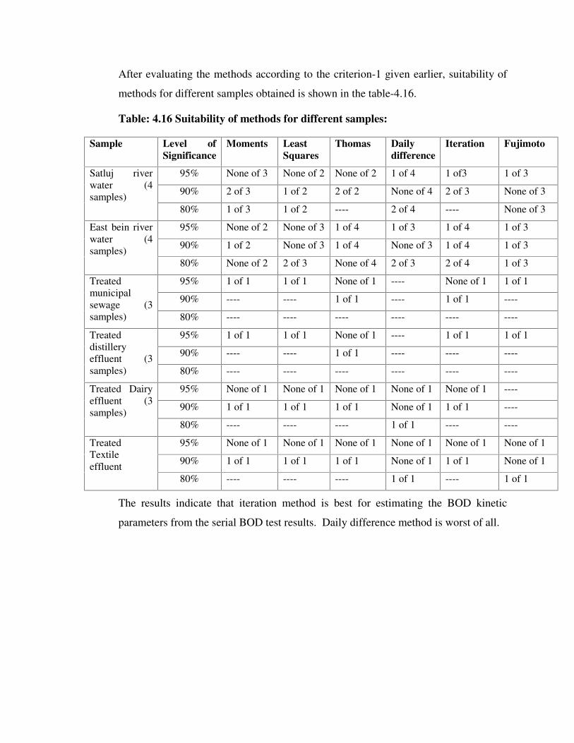
After evaluating the methods according to the criterion-1 given earlier, suitability of

methods for different samples obtained is shown in the table-4.16.

Table: 4.16 Suitability of methods for different samples:

Sample Level of Significance

Moments Least Squares

Thomas Daily difference

Iteration Fujimoto

95% None of 3 None of 2 None of 2 1 of 4 1 of3 1 of 3

90% 2 of 3 1 of 2 2 of 2 None of 4 2 of 3 None of 3

Satluj river water (4 samples)

80% 1 of 3 1 of 2 ---- 2 of 4 ---- None of 3

95% None of 2 None of 3 1 of 4 1 of 3 1 of 4 1 of 3

90% 1 of 2 None of 3 1 of 4 None of 3 1 of 4 1 of 3

East bein river water (4 samples)

80% None of 2 2 of 3 None of 4 2 of 3 2 of 4 1 of 3

95% 1 of 1 1 of 1 None of 1 ---- None of 1 1 of 1

90% ---- ---- 1 of 1 ---- 1 of 1 ----

Treated municipal sewage (3 samples) 80% ---- ---- ---- ---- ---- ----

95% 1 of 1 1 of 1 None of 1 ---- 1 of 1 1 of 1

90% ---- ---- 1 of 1 ---- ---- ----

Treated distillery effluent (3 samples) 80% ---- ---- ---- ---- ---- ----

95% None of 1 None of 1 None of 1 None of 1 None of 1 ----

90% 1 of 1 1 of 1 1 of 1 None of 1 1 of 1 ----

Treated Dairy effluent (3 samples)

80% ---- ---- ---- 1 of 1 ---- ----

95% None of 1 None of 1 None of 1 None of 1 None of 1 None of 1

90% 1 of 1 1 of 1 1 of 1 None of 1 1 of 1 None of 1

Treated Textile effluent

80% ---- ---- ---- 1 of 1 ---- 1 of 1

The results indicate that iteration method is best for estimating the BOD kinetic

parameters from the serial BOD test results. Daily difference method is worst of all.

4.5 Conclusions

Method of moments has been found erroneous under the following two different

conditions:

� When there is a lag phase in the serial BOD test (lag phase reduces the t value

(from 7 to 7-lag period) where as the nomogram used is specific for t=7 days)

� When the sample is a river water sample or when it is thoroughly treated

effluent sample k value obtained by Method of Moments has been very low

and the L0 value very high (consistently higher than the sample’ s COD)

Results of the serial BOD tests have been observed to be not of that high accuracy

and dependable. Accurate results might have made the study much more useful.

The evaluation approach followed in this study has indicated that Iteration method is

the best and daily difference method the worst among the methods evaluated for

estimating BOD kinetics parameters from the serial BOD test results.

Fig: 4.1 Method comparison for SAT-7(I)

0

1

2

3

4

5

6

7

0 1 2 3 4 5 6 7 8

Days

BO

D(m

g/l)

Observed BOD

Moments(0.83)

Least squares(1.13)

Thomas(0.62)

Daily diff.(2.98)

Iteration(0.64)

Fujimoto(1.59)

BOD = 6.56 mg/lCOD = 16 mg/l

Fig: 4.2 Method comparison for SAT-7 (II)

0

1

2

3

4

5

6

7

0 1 2 3 4 5 6 7 8Days

BO

D (m

g/l)

Observed BOD

Moments(0.15)

Least squares(0.18)

Thomas(0.37)

Daily diff.(0.17)

Iteration(0.30)

Fujimoto(2.59)

BOD = 4.60 mg/lCOD = 21.0 mg/l

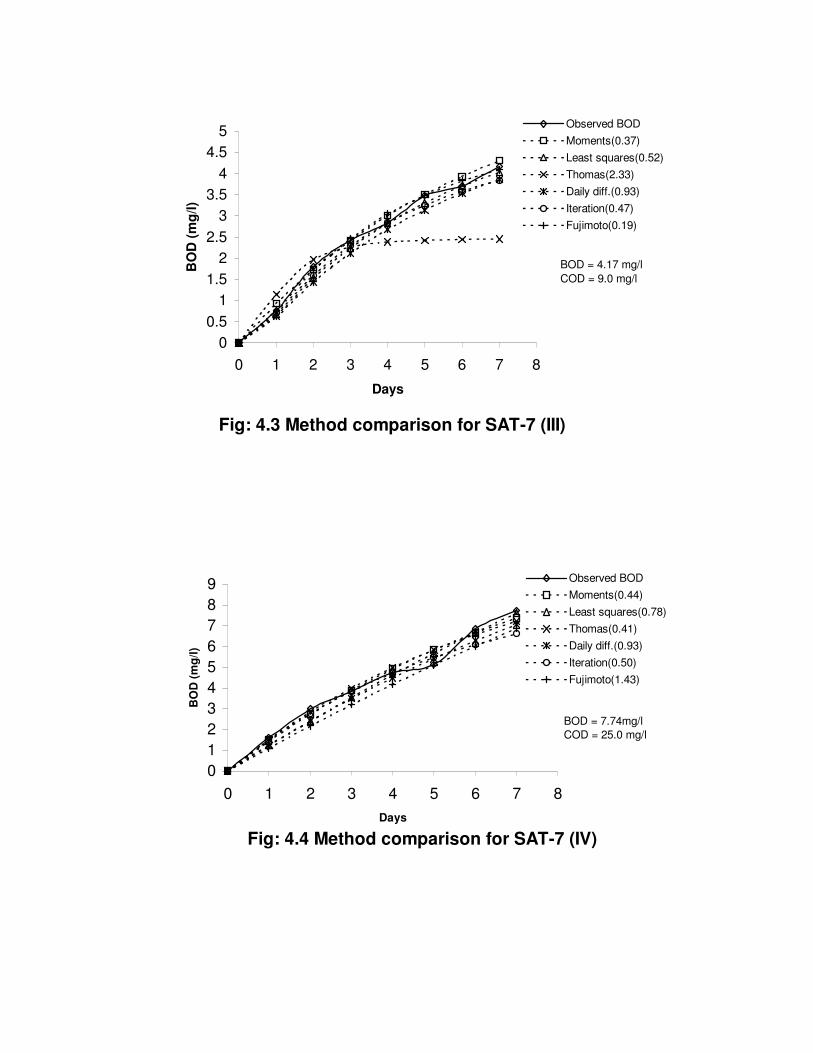
Fig: 4.3 Method comparison for SAT-7 (III)

00.5

11.5

22.5

33.5

44.5

5

0 1 2 3 4 5 6 7 8

Days

BO

D (m

g/l)

Observed BODMoments(0.37)Least squares(0.52)Thomas(2.33)Daily diff.(0.93)Iteration(0.47)Fujimoto(0.19)


Fig: 4.4 Method comparison for SAT-7 (IV)

0123456789

0 1 2 3 4 5 6 7 8Days

BO

D (m

g/l)


BOD = 7.74mg/lCOD = 25.0 mg/l

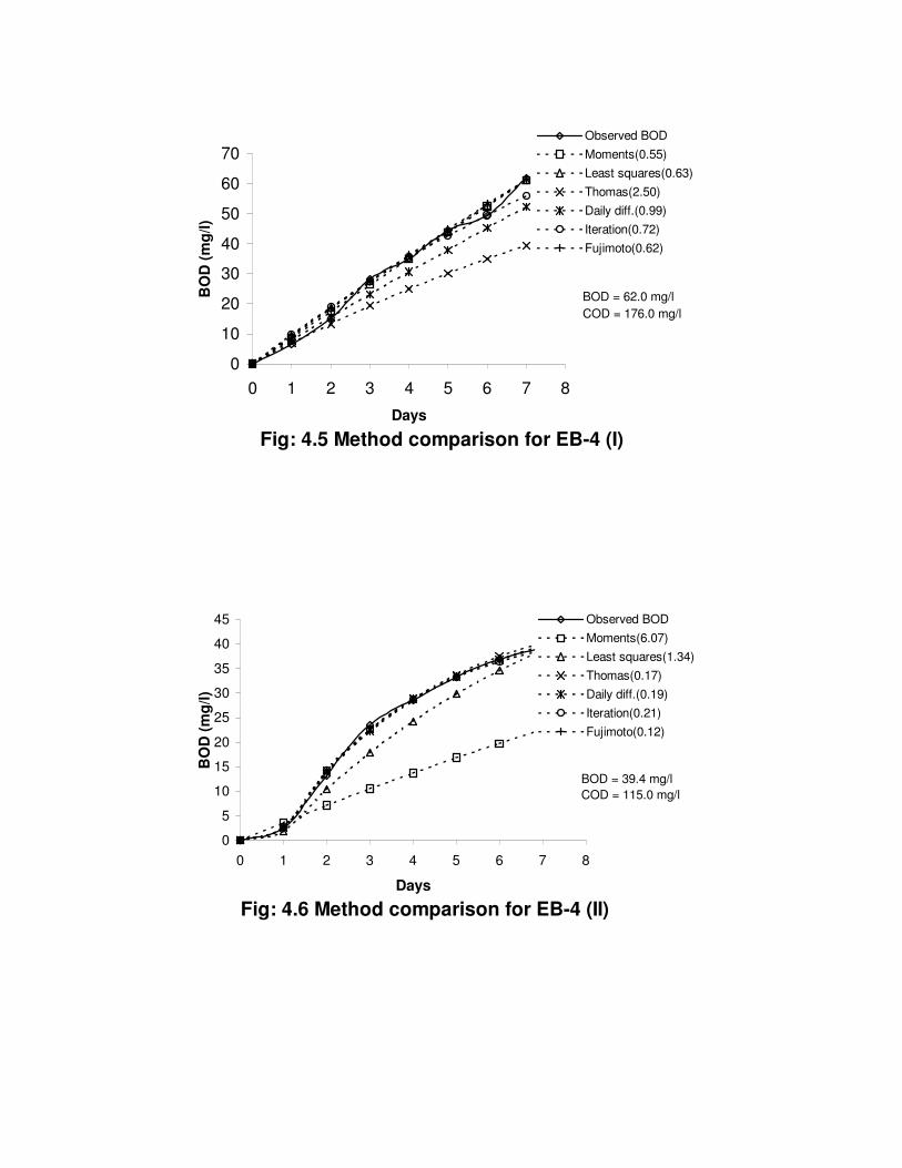
Fig: 4.5 Method comparison for EB-4 (I)

0

10

20

30

40

50

60

70

0 1 2 3 4 5 6 7 8

Days

BO

D (m

g/l)


BOD = 62.0 mg/lCOD = 176.0 mg/l

Fig: 4.6 Method comparison for EB-4 (II)

0

5

10

15

20

25

30

35

40

45

0 1 2 3 4 5 6 7 8

Days

BO

D (m

g/l)


BOD = 39.4 mg/lCOD = 115.0 mg/l

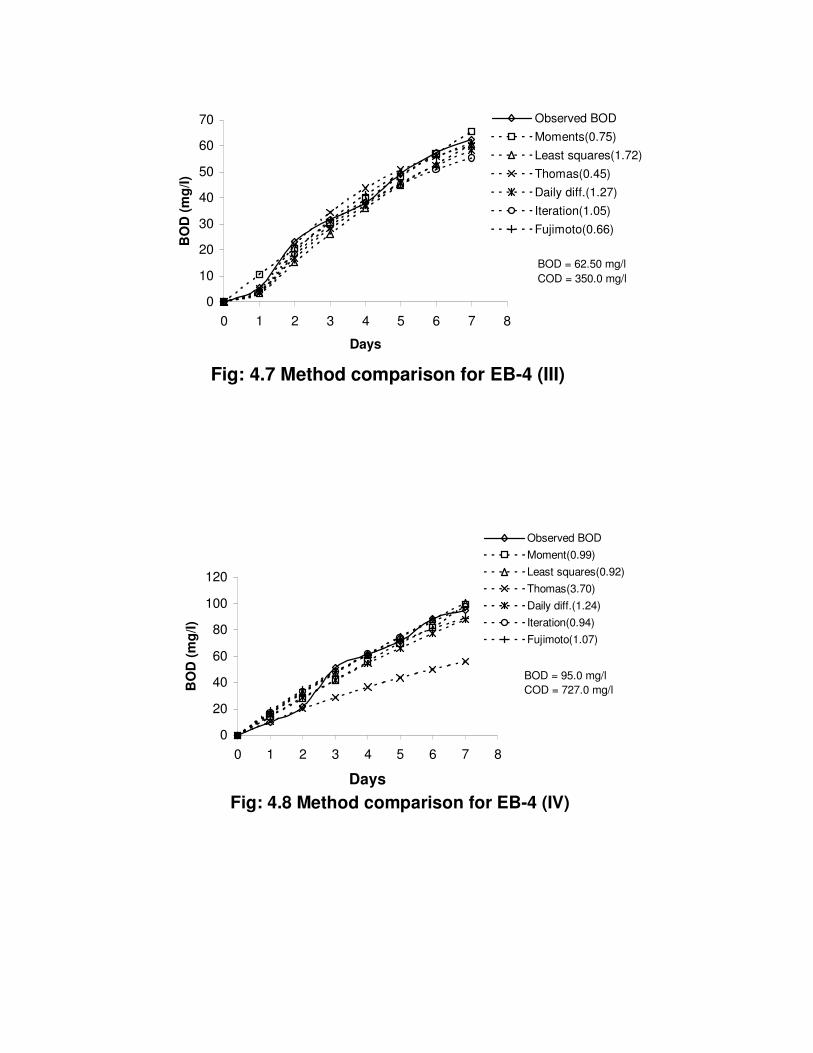
Fig: 4.7 Method comparison for EB-4 (III)

0

10

20

30

40

50

60

70

0 1 2 3 4 5 6 7 8

Days

BO

D (m

g/l)


BOD = 62.50 mg/lCOD = 350.0 mg/l

Fig: 4.8 Method comparison for EB-4 (IV)

0

20

40

60

80

100

120

0 1 2 3 4 5 6 7 8

Days

BO

D (m

g/l)

Observed BODMoment(0.99)Least squares(0.92)Thomas(3.70)Daily diff.(1.24)Iteration(0.94)Fujimoto(1.07)

BOD = 95.0 mg/lCOD = 727.0 mg/l

Fig. 4.9 Method comparison for sewage-I

0

10

20

30

40

50

0 1 2 3 4 5 6 7 8Days

BO

D(m

g/l)

Observed BOD

Moments(0.32)

Least squares(0.34)

Thomas(0.40)

Daily diff.(0.67)

Iteration(0.73)

Fujimoto(0.31)BOD = 37.8 mg/lCOD = 125.0 mg/l

Fig: 4.10 Method comparison for Sewage - II

0

50

100

150

200

250

0 1 2 3 4 5 6 7 8Days

BO

D(m

g/l)


BOD = 188.0 mg/lCOD = 160.0 mg/l

Fig: 4.11 Method comparison for Sewage-III

020406080

100120140160180200

0 1 2 3 4 5 6 7 8

Days

BO

D(m

g/l)

Observed BOD

Moments(0.22)

Least squares(0.22)

Thomas(0.14)

Daily diff.(0.16)

Iteration(0.41)

Fujimoto(0.36)

BOD = 183.0 mg/lCOD = 180.0 mg/l

Fig. 4.12 Method comparison for Distillery-I

0500

100015002000250030003500400045005000

0 1 2 3 4 5 6 7 8Days

BO

D(m

g/l)

Observed BOD

Moments(0.49)

Least squares(0.64)

Thomas(0.47)

Daily diff.(0.96)

Iteration(0.57)

Fujimoto(1.18)

BOD = 4650.0 mg/lCOD = 5000.0 mg/l

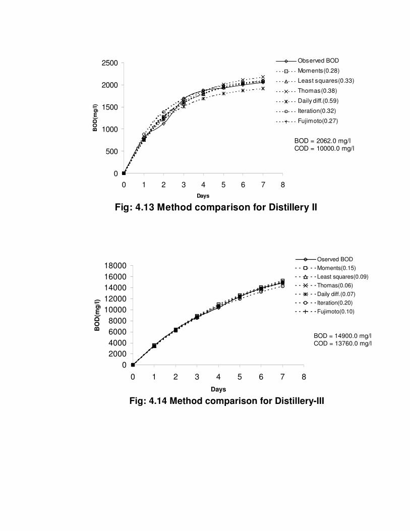
Fig: 4.13 Method comparison for Distillery II

0

500

1000

1500

2000

2500

0 1 2 3 4 5 6 7 8Days

BO

D(m

g/l)

Observed BOD

Moments(0.28)

Least squares(0.33)

Thomas(0.38)

Daily diff.(0.59)

Iteration(0.32)

Fujimoto(0.27)

BOD = 2062.0 mg/lCOD = 10000.0 mg/l

Fig: 4.14 Method comparison for Distillery-III

02000400060008000

1000012000140001600018000

0 1 2 3 4 5 6 7 8Days

BO

D(m

g/l)

Oserved BODMoments(0.15)Least squares(0.09)Thomas(0.06)Daily diff.(0.07)Iteration(0.20)Fujimoto(0.10)

BOD = 14900.0 mg/lCOD = 13760.0 mg/l

Fig: 4.15 Method comparison for Dairy-I

020406080

100120140160180200

0 1 2 3 4 5 6 7 8

Days

BO

D(m

g/l)

Observed BOD

Moments(0.38)

Least squares(0.86)

Thomas(0.32)

Daily diff.(2.03)

Iteration(0.35)

Fujimoto(0.52)

BOD = 178.5 mg/lCOD = 200.0 mg/l

Fig: 4.16 Method comparison for Dairy-II

0102030405060708090

100

0 1 2 3 4 5 6 7 8Days

BO

D(m

g/l)

Observed BOD

Moments(0.71)

Least squares(0.25)

Thomas(0.70)

Daily diff.(0.35)

Iteration(0.31)

Fujimoto(0.56)

BOD = 82.0 mg/lCOD = 100.0 mg/l

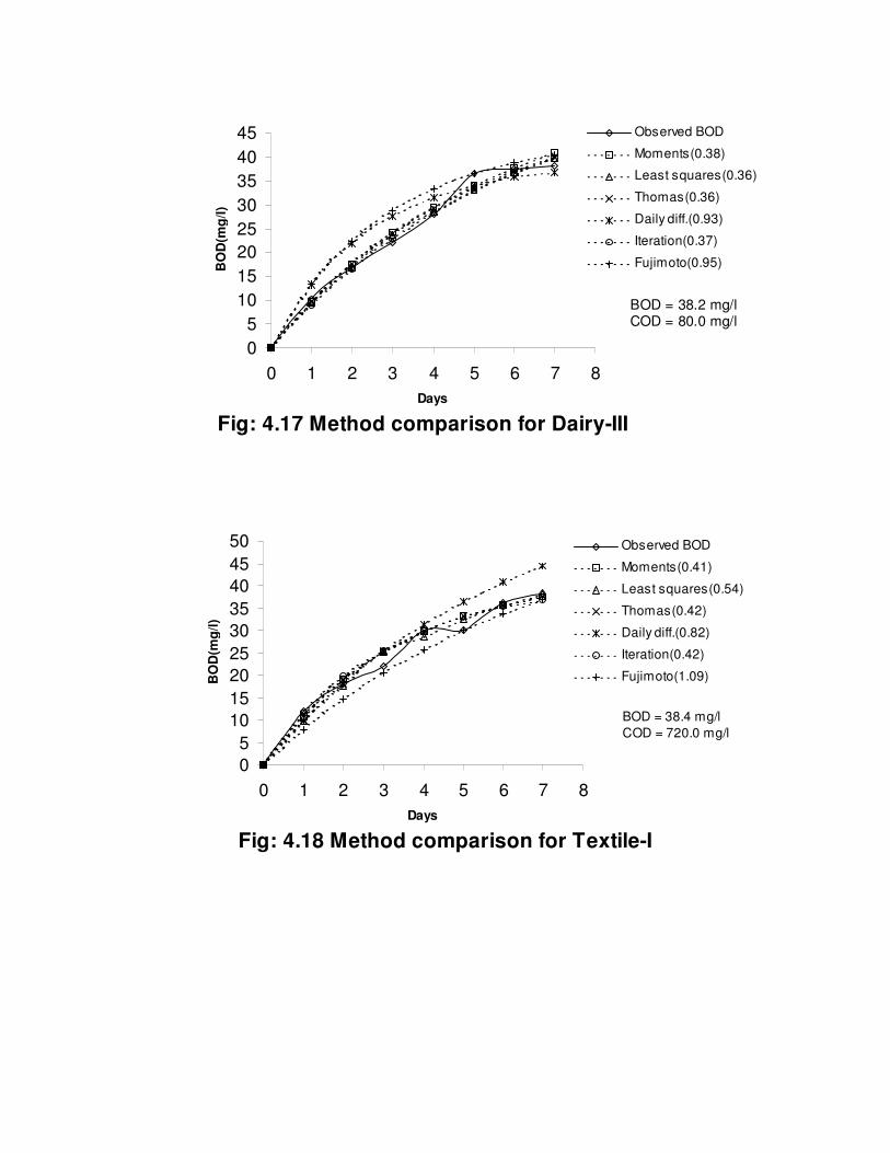
Fig: 4.17 Method comparison for Dairy-III

05

1015202530354045

0 1 2 3 4 5 6 7 8Days

BO

D(m

g/l)

Observed BOD

Moments(0.38)

Least squares(0.36)

Thomas(0.36)

Daily diff.(0.93)

Iteration(0.37)

Fujimoto(0.95)


Fig: 4.18 Method comparison for Textile-I

05

101520253035404550

0 1 2 3 4 5 6 7 8Days

BO

D(m

g/l)

Observed BOD

Moments(0.41)

Least squares(0.54)

Thomas(0.42)

Daily diff.(0.82)

Iteration(0.42)

Fujimoto(1.09)

BOD = 38.4 mg/lCOD = 720.0 mg/l

Fig: 4.19 Method comparison for Textile-II

0

500

1000

1500

2000

2500

0 1 2 3 4 5 6 7 8Days

BO

D(m

g/l)

Observed BOD

Moments(0.15)

Least squares(0.18)

Thomas(0.37)

Daily diff.(0.17)

Iteration(0.30)

Fujimoto(2.59)

BOD = 1693.6 mg/lCOD = 1300.0 mg/l

Fig: 4.20 Method comparison for Textile-III

-500

0

500

1000

1500

2000

2500

3000

3500

4000

4500

0 1 2 3 4 5 6 7 8

Days

BO

D(m

g/l)

Observed BOD

Moments(1.47)

Least squares(1.37)

Thomas(0.74)

Daily diff.(1.74)

Iteration(0.73)

Fujimoto(0.69)

BOD = 3795.0 mg/lCOD = 2000.0 mg/l

CHAPTER: 5

Conclusions

The present study on the evaluation of six different methods for BOD kinetic

parameters estimation, while using the serial BOD test results for treated industrial

effluents and river waters, has indicated that Iteration method is the best and Daily

difference method is the worst. This conclusion should be seen in the light of the

following limitations of the present study:

1. BOD and COD results indicate that some of the samples used in the study are not

in real sense treated effluents (at the time sampling the treatment plant might not

been working satisfactorily) (sewage samples 2 and 3, distillery effluent sample 3

and textile effluent sample 2 and 3).

2. In quite a few cases the testing has indicated that their BOD7 is greater than COD

– this indicates that the testing of the samples has not been that accurate. For

making the evaluation process acceptable the results of all such samples whose

BOD7 was obtained greater than the COD have not been considered.

3. In some of the cases in the serial BOD test, an initial lag phase was observed

(indicating that the seed used was not sufficiently acclimatized). For taking care

of this problem the BOD kinetic equation used has been appropriately modified.

But this modification has brought in certain errors affecting the evaluation

process.

4. Treated effluent samples have been used and for properly treated effluents k

values, as expected, have been found to be very low and wherever very low k

values are encountered the L0 was found to be higher than COD. Samples with

such cases have also been not considered in the evaluation process.

For the selection of appropriate method for BOD kinetic parameters, study has

indicated that the following aspects may be given due consideration:

� Serial BOD test may be conducted accurately while using properly acclimatized

seed and the results may be crosschecked with COD test.

� For each type of wastewater or water samples the methods may be separately

evaluated and selected on the basis of statistically significant number of serial

BOD tests (at least 7 samples may be tested).

� Incubation period for serial BOD test was chosen as 7 days and this may be

followed because it can allow bio-oxidation of significant fraction of the organic

matter and nitrogenous BOD exertion may still not be significant. However in

case of treated effluent samples for avoiding nitrogenous BOD exertion

appropriate inhibitors may be used.

The present study has clearly indicated that Moments Method of kinetic parameters

estimation is not good for samples from surface water bodies and for thoroughly

treated secondary effluents. Keeping this in mind further work may be planned for

answering the question ‘which method is most appropriate under what conditions?

REFERENCES

1. APHA, AWWA and WPCF (1995), “Standard Methods for Estimation of

Water & Waste Water”, 19th addition, 1995, Jointly edited by Eaton, Andrew

D.; Clesceri, Lenore S. and Greenberg, Arnold E..

2. Berthouex, P. M. and Hunter, W.G. (1971), “Problems associated with planning

BOD experiments”. J. San. Eng. Div. Amer. Soc. Civil Engr., 97 (SA4), p. 393-

407.

3. Booki Min; David Kohlar; Bruce E. Logan (2004), “A Simplified HBOD Test

Protocol Based on Oxygen Measurement using a fiber optic Probe”, Water

Environmental Research, Vol. 76(1), p. 29-36.

4. Bruce E. Logan; Gretchen A. Wagenseller (1993),”The HBOD Test: A New

Method for Determining Biochemical Oxygen Demand”, Water Environmental

Research, Vol. 65(7), p. 862.

5. Fair, G.M. (1936) “The Log Difference Method of Estimating the Constants of

the First Stage BOD Curve” Sewage Works Journ., Vol. 8, p. 430 – 434.

6. Fujimoto, Y (1961), “Graphical use of first stage BOD equation”, J. Water

Pollution Control, Vol. 36(1), p. 69.

7. Gaudy, A.F. Jr. (1972) “ Biochemical Oxygen Demand” in water Pollution

Microbiology Ed. Ralph Mitchell, Wiley Interscience N. Y. London, p. 305.

8. Guillermo Cutrera; Liliana Manfredi; Carlos E del Valle and Froilan Gonzalez, J.

(1999), “On the determination of the kinetic parameters for the BOD Test”,

Water SA, Vol. 25 No. 3, p. 377-379.

9. Gurjar, B. R. (1994), “Formulation of a Simple New Method to Determine

First – Stage BOD Constants, (K & L)” , Indian J. Environmental Protection,

Vol. 14, No. 6, p. 440-442.

10. Jenkins, D. (1960) “ The use of Manometric Methods in the Study of Sewage

and Trade Wastes” , in Waste Treatment Ed. P.C.G. Issac., p.319.

11. Le Blanc, P.J. (1974) “ Review of Rapid BOD Test Methods” , J. Water

Pollution Control Federation. Vol. 46, p. 2202.

12. Maiti, S.K. and Ganguly Sangeeta (2002) “ Errors in the Performance of

BOD327 and BOD5

20 test and its Effect on Determination of Rate Constant”

Indian J. Environmental Protection, Vol. 22 (10), p. 1113 – 1119.

13. Marske, D.M. and L.B. Polkowski (1972), “ Evaluation of methods for

estimating biochemical oxygen demand parameters”. J. Water Poll. Cont.

Fed., 44 (10), p. 1987-2000.

14. McGhee, T.J. (1991) “ Water Supply and Sewrage” 6th edition McGraw Hill,

Tokyo.

15. Metcalf Eddy (2003), “ Wastewater Engineering”, Tata McGraw Hill

Publication, New Delhi.

16. Moore, E. W.; Thomas; H. A., and Snow, W.B. (1950), “ Simplified Method for

analysis of BOD data”, Sew. Ind. Wastes. 22 (10).

17. Nesarattnam Suresh (1998), “ Effluent Treatment”, Pira Environmental Guide

Series, published by Pira International UK.

18. Phelps, E.B. (1953) “ Stream Sanitation” , Wiley, New York.

19. Peavy H.S., Donal R. Rowe, George Tchobanoglous (1985) “ Environmental

Engineering” McGraw Hill, New York p. 43

20. Rai, R. K. (2000), “ Simplified method for Determination of BOD Constants” ,

Indian J. Environmental Protection, Vol. 20, No. 4, p. 263-267.

21. Rai, R. K. (2000), “ Iteration Method For The Analysis Of BOD Data” , Indian

J. Environmental Health. Vol. 42. No. 1 p. 25-27.

22. Ramallho, R. S. (1983), “ Introduction to Wastewater Treatment Process” ,

Academic Publication, (Second Edition), New York.

23. Reddy, A. S., “ BOD and BOD kinetics” , Under Publication.

24. Reed, L.J. and Theriault, E.J. (1931), “ The statistical treatment of reaction” .

Velocity data – II. J. Phys. Chem., p. 35 – 950.

25. Remo Navone (1960), “ A new method for calculating k and L for sewage” ,

Water and Sewage Works, p. 285-286.

26. Shrivastava, A.K. (1982) “ Analytical and Experimental Investigations of BOD

Kinetics in an Aquatic Eco-systems” Ph. D. Thesis submitted to University of

Roorkee, Roorkee.

27. Shrivastva, A.K.: Swaroop Jyoti and Jain Neeraj (2000), “ Effect of Indigenous

Seed on Kinetic Equations” , Indian J. Environmental health, Vol.22(2), p. 75-

78.

28. Stone, T. (1981), “ A resume of the Kinetics of BOD Test”, Water Pollution

Control 80(4), p. 513-520.

29. Thomas, Jr. H.A. (1937) “ The Slope Method of Evaluating the Constants of

the First Stage BOD Curve” Sewage Works J., Vol. 9, p. 425.

30. Thomas, H.A. (1950), “ Graphical determination of BOD curve constants” ,

Water & Sewage works, Vol. 97, p. 123.

31. William, E. Gates and Sambhunath Ghosh (1971) “ Biokinetic Evaluation of

BOD Concepts and Data” J. Sanitary Engineering Division, SA-3, p. 287 – 307.

Documents

Bod Methods Best