BOAST98-MC Final Report & Users Manual - Advanced Resources

Advanced Resources InternationalAdvanced Resources International

BOAST 98-MC: A Probabilistic Simulation Module for BOAST 98 Final Report and Users Manual Aiysha Sultana, Anne Oudinot, Reynaldo Gonzalez and Scott Reeves Advanced Resources International 9801 Westheimer Rd, Suite 805 Houston, TX 77042 U.S. Department of Energy DE-FC26-04NT15528 June, 2006

Advanced Resources International, Inc. AO062006

i

Disclaimers

U.S. Department of Energy This report was prepared as an account of work sponsored by an agency of the United States Government. Neither the United States Government nor any agency thereof, nor any of their employees, makes any warranty, express or implied, or assumes any legal liability or responsibility for the accuracy, completeness, or usefulness of any information, apparatus, product or process disclosed, or represents that its use would not infringe privately owned rights. Reference herein to any specific commercial product, process, or service by trade name, trademark, manufacturer, or otherwise does not necessarily constitute or imply its endorsement, recommendation, or favoring by the United States Government or any agency thereof. The views and opinions of authors expressed herein do not necessarily state or reflect those of the United States Government or any agency thereof.

Advanced Resources International The material in this Report is intended for general information only. Any use of this material in relation to any specific application should be based on independent examination and verification of its unrestricted applicability for such use and on a determination of suitability for the application by professionally qualified personnel. No license under any Advanced Resources International, Inc., patents or other proprietary interest is implied by the publication of this Report. Those making use of or relying upon the material assume all risks and liability arising from such use or reliance.


ii

Abstract This work was performed by Advanced Resources International (ARI) on behalf of the United States Department of Energy (DOE) in order to develop a user-friendly, PC-based interface that couples DOE’s BOAST 98 software with the Monte Carlo simulation technique. The objectives of the work were to improve reservoir management and maximize oil recoveries by understanding and quantifying reservoir uncertainty as well as improving the capabilities of DOE’s BOAST 98 software by incorporating a probabilistic module in the simulator. In this model, probability distributions can be assigned to unknown input parameters such as permeability, porosity, etc. Options have also been added to the input file to be able to vary relative permeability curves as well as well spacing. Hundreds of simulations can then automatically be run to explore the many combinations of uncertain reservoir parameters across their spectrum of uncertainty. Output data such as oil rate and water rate can then be plotted. When historical data are available, they can be uploaded and a least-square error-function run between the simulation data and the history data. The set of input parameters leading to the best match is thus determined. Sensitivity charts (Tornado plots) that rank the uncertain parameters according to the impact they have on the outputs can also be generated.


iii

Table of Contents Disclaimers.................................................................................................................................................... i Abstract ........................................................................................................................................................ ii Table of Contents ........................................................................................................................................ iii List of Tables............................................................................................................................................... iv List of Figures ...............................................................................................................................................v 1.0 Introduction ......................................................................................................................................1 2.0 Model Description............................................................................................................................2

2.1 Installation....................................................................................................................................2 2.2 Running the Model.......................................................................................................................2 2.2.1 Welcome Screen ..........................................................................................................................2 2.2.2 Input Panel ...................................................................................................................................2 2.2.3 Generating the Boast98 Input File ...............................................................................................4 2.2.4 Defining Uncertainties and Outputs.............................................................................................9 2.2.5 Actual Data ................................................................................................................................12 2.3 Results........................................................................................................................................13 2.3.1 Creating Plots.............................................................................................................................13 2.3.2 Error Function ............................................................................................................................15 2.3.3 Sensitivity Charts .......................................................................................................................17 2.4 Project Management ..................................................................................................................18

3.0 Example..........................................................................................................................................19

3.1 Model Description......................................................................................................................19 3.2 Input Variables...........................................................................................................................19 3.3 Results........................................................................................................................................20

4.0 Conclusions ....................................................................................................................................24

5.0 References ......................................................................................................................................24

Appendix A: Source Code........................................................................................................................ A-1

Appendix B: Executable File.....................................................................................................................B-1

Appendix C: Example Files.......................................................................................................................C-1


iv

List of Tables

Table 1: Input Data Distribution Parameters...............................................................................................20


v

List of Figures Figure 1: Boast98-MC Welcome Screen.......................................................................................................2 Figure 2: Open File Screen Shot ...................................................................................................................3 Figure 3: Warning Screen Shot .....................................................................................................................3 Figure 4: Screen Shot: Instructions Worksheet .............................................................................................4 Figure 5: Screen Shot: Input File Worksheet ...............................................................................................5 Figure 6: Screen Shot: Automatic Gridding ..................................................................................................6 Figure 7: Screen Shot: Probability Distribution Options.............................................................................10 Figure 8: Screen Shot: Project Informations ...............................................................................................11 Figure 9: Screen Shot: History Tab .............................................................................................................12 Figure 10: Screen Shot: Data Upload and Transfer.....................................................................................13 Figure 11: Screen Shot: Plot Data Selection Tab ........................................................................................14 Figure 12: Screen Shot: Plot Tab.................................................................................................................15 Figure 13: Screen Shot: Error Function.......................................................................................................16 Figure 14: Screen Shot: Sensitivity Chart ...................................................................................................17 Figure 15: Example of Tornado Plot ...........................................................................................................18

Figure 16: Screen Shot: Exit Tab ................................................................................................................18 Figure 17: Example Model..........................................................................................................................19 Figure 18: Gas Production Rate Chart.........................................................................................................20 Figure 19: Cumulative Gas Production Chart .............................................................................................21 Figure 20: Oil Production Rate Chart..........................................................................................................21 Figure 21: Cumulative Oil Production Chart ..............................................................................................22 Figure 22: Error Function Results ...............................................................................................................22 Figure 23: Cumulative Gas Production Tornado Chart...............................................................................23

Figure 24: Sensitivity Chart Output: Cumulative Gas Production ..............................................................23

Figure 25: Cumulative Oil Production Tornado Chart ................................................................................24


1

1.0 Introduction This work was performed by Advanced Resources International (ARI) on behalf of the United States Department of Energy (DOE) in order to develop a user-friendly, PC-based interface that couples DOE’s BOAST98 software with the Monte Carlo simulation technique. The objectives of the work were to improve reservoir management and maximize oil recoveries by understanding and quantifying reservoir uncertainty as well as improving the capabilities of DOE’s BOAST98 software by incorporating a probabilistic module in the simulator. In this model, probability distributions can be assigned to unknown input parameters such as permeability, porosity, etc. Options have also been added to the input file to be able to vary relative permeability curves as well as well spacing. Hundreds of simulations can then automatically be run to explore the many combinations of uncertain reservoir parameters across their spectrum of uncertainty. Output data such as oil rate and water rate can then be plotted. When historical data are available, they can be uploaded and a least-square error-function run between the simulation data and the history data. The set of input parameters leading to the best match is thus determined. Sensitivity charts (Tornado plots) that rank the uncertain parameters according to the impact they have on the outputs can also be generated. This report gives detailed instructions on how to use the model and serves as the Users Manual for it. The BOAST98 users manual is accessible from the model for specific questions about the simulator.


2

2.0 Model Description 2.1 Installation The installation only requires a few steps. • Double-click the Setup.exe file. • Follow the instructions provided by the Setup wizard. • All the files will be located under C:\Program Files\Boast98 • Double click the BOAST98-MC.exe to start the model. 2.2 Running the Model This section describes step by step how to use this model, specifically how to create the BOAST98 input file, specify probability distributions, define outputs, create the historical data file and run the simulations as well as looking at output data, generating sensitivity charts and running the error function when actual data are available. 2.2.1 Welcome Screen When the BOAST98-MC.exe is launched, the welcome screen shown on Figure 1 is displayed. Press the ‘Continue’ button.

Figure 1: BOAST98-MC Welcome Screen 2.2.2 Input Panel The screen shown on Figure 2 appears when the ‘Continue’ button is pressed. The first step in the process is to open the BOAST98 input file. To do so, the version of Microsoft Office installed on the computer first has to be determined. Then select from the


3

dropdown menu a previously created project or create a new one by typing in the name in the provided space. When a new project is created from that panel, all the necessary files are copied from the ‘Sample’ folder that contains all necessary template files. In order to prevent some files from being overwritten, if an existing project is selected, the screen shown on Figure 3 will be displayed, after the ‘Launch Input File’ button is pressed.

Figure 2: Open File Screen Shot

Figure 3: Warning Screen Shot


4

A new project can be created at this point (with all the necessary files copied from the existing project) or the selected project can simply be opened. 2.2.3 Generating the BOAST98 input file An exact copy of a BOAST98 input file has been created in Excel and serves as a template to make modifications pertinent to the actual project. This Excel file is composed of six worksheets:

Instructions The ‘Instructions’ worksheet gives essential explanations to the user to be able to run the model. If more explanations are required, the user will then have to refer to this manual or to the BOAST98 manual. Two buttons located on the worksheet directly link to both manuals as shown on Figure 4. Please read these instructions carefully before doing any changes to the input file as special features have been added to the regular BOAST98 input file.

Figure 4: Screen Shot: Instructions Worksheet

InputFile The ‘InputFile’ worksheet is an exact copy of a BOAST98 input file. The user only has to read through the file and change the input parameters according to the particular case being studied. In order to make this process easier, comments have been added to each input data. Cells with comments can be recognized by the red triangle located at the upper right corner of the cell as shown on Figure 5. By just bringing the mouse above the triangle, the comments will show up.


5

Figure 5: Screen Shot: Input File Worksheet Recurrent Data Section In the recurrent data section, two rows regarding the well characteristics and rates demand particular attention. In order to be able to run with BOAST98, those two lines need to have a special Fortran formatting. These instructions have to be followed rigorously. The first line (well characteristics) is as follows. WELLID IDWELL I J PERF1 NLAYER The first parameter, WELLID, is in format A5, meaning 5 ASCII characters. The well name can only be five-character and subsequent parameters should begin after column five. The next 5 parameters are in format I3 so each parameter can only be 3 characters long. As a consequence, the last digit of the IDWELL should be in column 8, the last digit of I in column 11, the last digit of J in column 14, the last digit of PERF1 in column 17 and the last digit of NLAYER in column 20. The second line (rate control and rate information) is as follows: WELLID IDWELL KIP QO QW QG QT As for the well characteristics, WELLID is in formal A5. IDWELL and KIP are in format I3. So IDWELL should end in column 8 and KIP in column 11. The last 4 parameters are in format F10.0, meaning 10 digits with no digit after the decimal point. The last character of QO should be in column 20 (including the decimal point), the last character of QW in column 30, the last character of QG in column 40 and the last character of QT in column 50.


6

Because of the constraints on the way these numbers have to be displayed, these two lines will be included in one cell instead of one parameter per cell. As a consequence, no probability distribution can be assigned to any of those parameters.

AutomaticGrid A special worksheet has been created regarding the reservoir model grid. Four codes are used to input the grid dimensions (KDX, KDY, KDZ and KDZNET). This section of the input data for BOAST98 has been slightly modified to add an automatic gridding option. If KDX=-1 (or KDY=-1), the grid dimensions are the same for all the blocks in the considered direction, and only one value has to be input. Those values can be directly entered on the InputFile worksheet or they can also be input on the Automatic Grid worksheet. Clicking on the ‘Okay’ button will copy these values to the input sheet and make sure that eventual previous values are cleared and KDX and KDY set to –1. An option has been added to the BOAST98 input file, which will automatically create a grid, for a ‘one well case’ only. The well will be located in the center of the grid, which will be square. On the ‘AutomaticGrid’ worksheet, click on the ‘Automatic Grid’ button. A window will pop-up (Figure 6), asking the user for the well spacing, the length of the grid block in which the well will be located as well as an increment factor to compute the length of consecutive gridblocks.

Figure 6: Screen Shot: Automatic Gridding

Click on the ‘Generate Grid’ and the values will appear in a table below. If the computed values are to be used for the simulation, click on the ‘Okay’ button and those values will be automatically entered on the InputFile worksheet after the previous values have been


7

cleared, KDX and KDY will be set to 0 and the number of blocks in the X and Y direction will also be input. If KDX=0 (or KDY=0) and no automatic gridding is to be used, the dimensions are reread for each grid block in the first row (in the first column). The same dimensions are assigned to all other rows (columns) and all other layers. Please fill in the provided table and click on the ‘Okay’ button. This will automatically clear the previous values, copy the values and set KDX and KDY to 0. Those values can also directly be input on the ‘InputFile’ worksheet itself. If KDX=1 (or KDY=1), the grid dimensions have to be read for each grid block in the first layer. The same dimensions will be assigned to all other layers. For this case, please input directly the data to the InputFile worksheet.

RelativePermeability A special worksheet has been created regarding relative permeability curves. In this model, analytical equations are used to approximate relative permeability curves. Those equations are detailed below. The main objective of this worksheet is to allow the user to vary those parameters and be able to see how the curves respond to those variations.

Oil phase relative permeability:

where Krow is the relative permeability of oil Sw is the water saturation Sorw is the residual oil to waterflood Swir is the irreducible water saturation Krocw is the endpoint (maximum) relative permeability of oil at the irreducible water saturation. Expow is the oil equation exponent.

Water phase relative permeability:

where

Expw

SorwSwirSwirSwKwroKrw ⎟

⎠⎞

⎜⎝⎛

−−−=

1

Expow

SorwSwirSorwSwKrocwKrow ⎟

⎠⎞

⎜⎝⎛

−−−−=

11


8

Krw is the relative permeability of water Sw is the water saturation Swir is the irreducible water saturation Sorw is the residual oil to waterflood Kwro is the endpoint (maximum) relative permeability of water at the residual oil saturation. Expw is the water equation exponent.

Gas phase relative permeability:

where Krg is the relative permeability of gas Sg is the gas saturation Sgr is the residual gas saturation to an oilflood Swir is the irreducible water saturation Krgcw is the endpoint (maximum) relative permeability of gas at the irreducible water saturation. Expg is the gas equation exponent.

Oil phase relative permeability in the presence of gas:

where Krog is the relative permeability of oil Swir is the irreducible water saturation Sorg is the residual oil to a gas flood Sg is the gas saturation Krocw is the endpoint (maximum) relative permeability of oil at irreducible water saturation. Expog is the oil equation exponent. The advantage of using those equations is to be able to define assumptions on those parameters so that relative permeability curves can change at each simulation. Of course, if a set of relative permeability curves is to be used for all the simulations, it is simply done by not defining any assumption on those parameters.

Expg

SgrSwirSgrSgKrgcwKrg ⎟⎟

⎠

⎞⎜⎜⎝

⎛−−

−=1

Expog

SorgSwirSgSorgSwirKrocwKrog ⎟⎟

⎠

⎞⎜⎜⎝

⎛−−

−−−=1

1


9

Note: in the table, SAT refers to the saturation of each particular phase. In a line where SAT=0.35, KROW refers to the oil relative permeability in presence of 35% oil saturation, KRW to the water relative permeability in presence of 35% water saturation, KRG to the gas saturation in presence of 35% gas saturation and KROG to the oil relative permeability in presence of 35% fluid (oil plus irreducible water) saturation. On the ‘RelativePermeability’ worksheet, the only values that can be changed are in red. When all the necessary values have been input, click the ‘Results’ button, the table as well as the plots will be updated. If those specific curves are to be used for the simulation, please click the ‘Export Results’ button and the calculated values will be automatically exported to the ‘InputFile’ worksheet. Of course, values can directly be entered on the ‘InputFile’ worksheet, knowing that the formulas in the table will then be lost for this specific project.

History_Data The ‘History_Data’ worksheet allows transferring actual production data to the database to be used later to compute the error function. Explanations on that process are provided in section 2.2.5 of the manual.

InputVariables The ‘InputVariables’ worksheet keeps track of the parameters related to the probability distributions defined on uncertain input parameters. 2.2.4 Defining uncertainties and outputs Once the input file has been generated, the next step is to define output parameters and distributions to the unknown input parameters by using the ‘Define Assumptions’ button on the ‘InputFile’ worksheet (Figure 7). If tornado plots are to be generated, the output parameters have to be defined first. Six parameters can be chosen as outputs: cumulative oil production, cumulative gas production, cumulative water production, average reservoir pressure (value at the end of the simulation), cumulative water injected and cumulative gas injected. By clicking the ‘Set Output Distributions’ button (Figure 7), the output parameters can be checked. The model will automatically keep track of the chosen outputs’ value at the end of each simulation in order to generate tornado plots. For uncertain input parameters, five probability distributions are available, Beta, Lognormal, Normal, Uniform and Triangular. Constraints for each distribution are also provided. With the cell to be varied selected, define the probability distribution as desired. The selected cell will turn bright pink in order to keep track of the varied parameters. Repeat the process for all the parameters to be varied and click ‘Finish’ when done.


10

An Excel file named ‘DataInput’ is being opened during the process. It keeps track of the name and cell references of the output and input parameters. For the input parameters, the types of distribution as well as the corresponding parameters (minimum and maximum or mean and standard deviation, etc.) are saved. The outputs are displayed in yellow and the inputs in green. The file will have to be saved and closed before starting the simulations. When the ‘Finish’ button is pressed, those data will be transferred to the DataInput worksheet on InputFile.xls for further reference.

Figure 7: Screen Shot: Probability Distribution Options


11

Before starting several simulations, it is advised to test the input file to ensure no errors have been generated while making modifications to the file. Click the ‘Test InputFile’ button. If the file has errors, a message from BOAST98 will pop-up. Please make the necessary changes until the file runs properly. Once the file is ready and running fine, it has to be saved using the ‘Save InputFile’ button. The screen shown on Figure 8 will then appear.

Figure 8: Screen Shot: Project Informations

The name of the project and the number of wells will already be entered. Please input the number of simulations to be run, choose the time increment for the simulations’ output data (daily, monthly or yearly) and select if the analysis is to be run on a field-basis only or on a field and wells basis. Click the ‘Save’ button. The process is now ready to be started. A message will open, asking the user to save and close the DataInput.xls file that got opened while defining output and input parameters. Once done, click the ‘Run Simulations’ button. If the model is used to try to history match real production data, the actual data can be entered before running the simulations or after as explained in section 2.2.5. A small window will stay open while the simulations are running to show the progress.


12

Note: Output data from a BOAST98 simulation are saved with time steps the same as the way the simulation has been running. In order to get daily, monthly or yearly data, interpolations are necessary to convert the data, which explains the time between simulations. 2.2.5 Actual Data If the model is used to try to history match real production data, those data have to be imported into the database. This is done under the ‘Actual_Data’ worksheet as shown on Figure 9. Using the dropdown menus provided, choose the start date and end date of the historical data. Choose the time increment (which has to be the same as the output data). By clicking the ‘Upload and Transfer Data’ button, the window shown on Figure 10 will appear. Click the ‘Retrieve Project’ button and all current existing projects will appear in the dropdown menu as well as the list of wells. Select the desired project and the well (or field) and click the ‘Upload’ button that will open the corresponding Excel file. The 2 first columns (date and days) will have been automatically filled in according to the data input earlier. Fill in each column with the actual data; input zeros when no data are available. When finished, save and close the file.

Figure 9: Screen Shot: History Data Click on the ‘Transfer’ button to export the data to the Access database. Repeat this process for each individual well if necessary and click ‘Finish’ when done.


13

Figure 10: Screen Shot: Data Upload and Transfer

2.3 Results: Plots and Error Function 2.3.1 Creating Plots On the interface, go to the ‘Plot Data Selection’ tab as shown on Figure 11. From the dropdown menu, select the project to be retrieved. This will have a list of all the projects contained in C:\Program Files\Boast98. Click on the ‘Retrieve’ button, the number of simulations that have been run will appear in the designed box. Then choose if plots are to be created for the field or for an individual well (option working only if this option was selected before running the simulations). From the dropdown menu, choose the parameter to be plotted. Are available for the field:

- Oil production rate - Gas production rate - Water production rate - Gas Oil ratio - Water Oil ratio - Gas injection rate - Water injection rate - Average reservoir pressure - Cumulative oil production - Cumulative gas production - Cumulative water production - Cumulative gas injection - Cumulative water injection

Are available for an individual well:

- Oil production rate - Gas production rate - Water production rate


14

- Gas injection rate - Water injection rate - Cumulative oil production - Cumulative gas production - Cumulative water production - Cumulative gas injection - Cumulative water injection - Oil saturation - Gas saturation - Water saturation - PWFC - PWFS

Figure 11: Screen Shot: Plot Data Selection Tab Click the ‘Set Scale’ button. This will find the minimum and maximum values for the X and Y axes of the plot. Select if you want to plot all the trials or just input the range of the desired trials. Go to the ‘Plot’ tab and click on the ‘Plot’ button as shown on Figure 12. All the curves from the simulations will be in blue; the curve for the actual data (if input earlier) will be in red. Each time a parameter is changed regarding the plot, click the ‘Clear Chart’ button, then the ‘Plot’ button, as it will not update by itself.


15

P10, P50 and P90 curves can also be added to the plot when selected from the list on the left hand side of the Plot tab. The Print button works like a ‘Print Screen’ option and will print the full panel with the chart.

Figure 12: Screen Shot: Plot Tab 2.3.2 Error Function This section explains how the error function is calculated between the actual data and the simulation data. The error function is as follows

∑∑

−−

−= 2

22

)()(

1MeanSimDataSimDataActualData

R

With

taNumberofDaActualData

Mean ∑=


16

In order to start a calculation, go to the ‘Error Function’ tab as shown on Figure 13. If the error function is to be computed for the field, under the field frame, choose the data under the dropdown menu and click the ‘Go’ button. If the error function is to be computed for a well, under the Well frame, first choose the well under the first dropdown menu, then the data under the second dropdown menu, then click the ‘Go’ button. Several error functions can be computed, but only the one after the other. The results will appear in the table. The header of each column will have the name of the well or field and the data. An ‘Export results to .csv’ button opens an Excel file (FinalOutput.xls). This file will have a summary table with the values randomly generated for each input parameter at each trial as well as the value(s) of the computed error function. Make sure before this process is started that actual production data have been uploaded to the database. Closer the error function is to 1.0, better is the match.

Figure 13: Screen Shot: Error Function


17

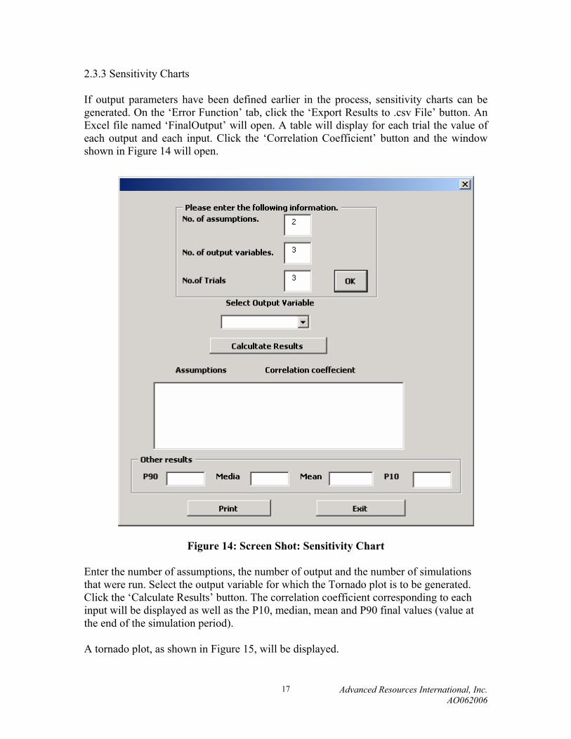
2.3.3 Sensitivity Charts If output parameters have been defined earlier in the process, sensitivity charts can be generated. On the ‘Error Function’ tab, click the ‘Export Results to .csv File’ button. An Excel file named ‘FinalOutput’ will open. A table will display for each trial the value of each output and each input. Click the ‘Correlation Coefficient’ button and the window shown in Figure 14 will open.

Figure 14: Screen Shot: Sensitivity Chart

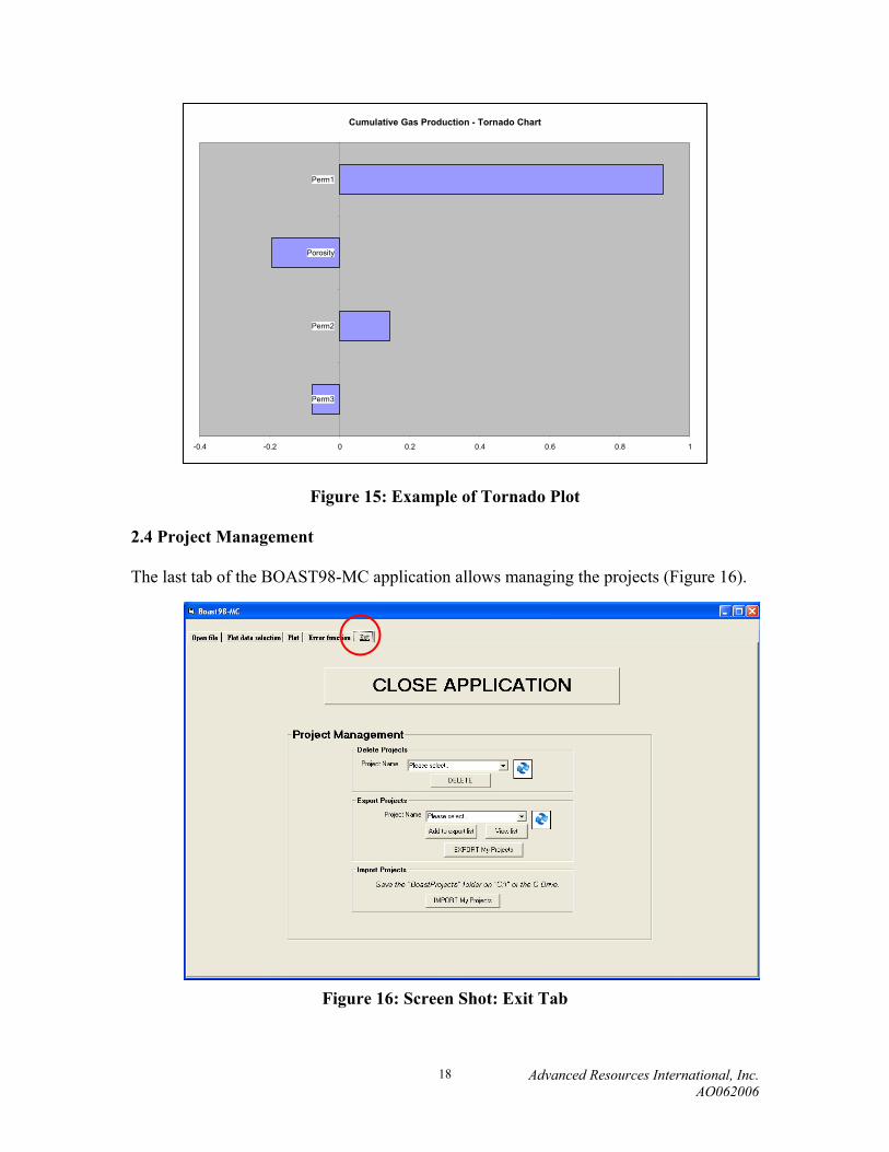
Enter the number of assumptions, the number of output and the number of simulations that were run. Select the output variable for which the Tornado plot is to be generated. Click the ‘Calculate Results’ button. The correlation coefficient corresponding to each input will be displayed as well as the P10, median, mean and P90 final values (value at the end of the simulation period). A tornado plot, as shown in Figure 15, will be displayed.


18

Figure 15: Example of Tornado Plot 2.4 Project Management The last tab of the BOAST98-MC application allows managing the projects (Figure 16).

Figure 16: Screen Shot: Exit Tab

Cumulative Gas Production - Tornado Chart

-0.4 -0.2 0 0.2 0.4 0.6 0.8 1

Perm3

Perm2

Porosity

Perm1


19

Projects can be deleted if necessary. The Export/Import option allows moving the projects from one computer to another. The Export option will transfer the selected projects to C:\BoastProjects. This folder just has to be copied to the C drive of the other computer. Then, clicking the IMPORT button will copy those projects to the appropriate folder on the new computer. The BOAST98-MC application can also be closed on this tab. 3.0 Example 3.1 Model Description The model studied is comprised of 2 wells (one producer and one injector) in a 10*10*3 grid, one well located in one corner, the other in the opposite corner (Figure 17). The injector is injecting gas in layer 1 only at 100,000 Mscfd while the producer produces from layer 3 with an oil rate constraint of 20,000 stbd for the first three years, which is then removed for the next seven years.

Figure 17: Example Model 3.2 Input Variables For this example, four input parameters were varied as shown in Table 1 below: permeability in layer 1, layer 2 and layer 3 as well as porosity. No anisotropy was considered so the permeability in the Y direction was set equal to the permeability in the X direction, which is easily done with the input file built in Excel.

INJ

PROD


20

Table 1: Input Data Distribution Parameters

Parameter Distribution Minimum Maximum Permeability Layer 1 Uniform 100 1000 Permeability Layer 2 Uniform 10 100 Permeability Layer 3 Uniform 100 500 Porosity Uniform 0.2 0.4 3.3 Results Twenty-five simulations were run for a period of ten years. Output data from a previous simulation were randomly chosen and used as actual data. The error function was then computed for both the oil rate and the gas rate. Figures 18 to 21 show the gas rate, oil rate, cumulative gas production and cumulative oil production from those 25 runs as well as the actual data and the P10, P 50and P90 curves.

Figure 18: Gas Production Rate Chart


21

Figure 19: Cumulative Gas Production Chart

Figure 20: Oil Production Rate Chart


22

Figure 21: Cumulative Oil Production Chart

Figure 22: Error Function Results


23

Figure 23: Cumulative Gas Production Tornado Chart

Figure 24: Sensitivity Chart Output: Cumulative Gas Production

Cumulative Gas Production - Tornado Chart

-0.4 -0.2 0 0.2 0.4 0.6 0.8 1

Perm3

Perm2

Porosity

Perm1


24

Figure 25: Cumulative Oil Production Tornado Chart Figures 19 and 21 show that, within the range defined for each uncertain parameter, cumulative gas production will fall between 350,000 MMscf and 450,000 MMscf whereas oil production will be between 35,000 Mstb and 95,000 MStb. The Tornado charts produced show that the permeability in layer 2 doesn’t have any impact on the production, allowing thus to remove that parameter from the list of the variables. 4.0 Conclusions A means of probabilistic forecasting and automatic history matching has been created through the use of a coupled stochastic module and reservoir simulator for characterization of black oil reservoirs. These techniques provide the flexibility to run nearly unlimited simulation cases in order to explore combinations of unknown parameters across their range of uncertainty for probabilistic forecasting and, if available, for comparison to historical data. Upon complexion, cases of interest are automatically high-graded. 5.0 References 1. Handbook for personal computer version of BOAST II: A three-dimensional, three-phase black oil applied simulation tool, Lori G. Stapp and Edith C. Allison, December 1989.

Cumulative Oil Production - Tornado Chart

-0.6 -0.4 -0.2 0 0.2 0.4 0.6 0.8

Perm2

Porosity

Perm1

Perm3


1

Appendix A: Digital Files

- Source Code

A -


1

Appendix B: Digital Files - Executable File

B -


1

Appendix C: Digital Files - Example Files

C -

Documents

BOAST98-MC Final Report & Users Manual - Advanced Resources