Board of Governors of the Federal Reserve System

International Finance Discussion Papers

Number 1065

November 2012

Interest Rates and the Volatility and Correlation of Commodity Prices

Joseph W. Gruber

Robert J. Vigfusson

NOTE: International Finance Discussion Papers are preliminary materials circulated to stimulate discussion and critical comment. References to International Finance Discussion Papers (other than an acknowledgment that the writer has had access to unpublished material) should be cleared with the author or authors. Recent IFDPs are available on the Web at www.federalreserve.gov/pubs/ifdp/. This paper can be downloaded without charge from Social Science Research Network electronic library at www.ssrn.com.

Interest Rates and the Volatility and Correlation of Commodity Prices

Joseph W. Gruber and Robert J. Vigfusson*

Abstract: We purpose a novel explanation for the observed increase in the correlation of commodity prices over the past decade. In contrast to theories that rely on the increased influence of financial speculators, we show that price correlation can increase as a result of a decline in the interest rate. More generally, we examine the effect of interest rates on the volatility and correlation of commodity prices, theoretically through the framework of Deaton and Laroque (1992) and empirically via a panel GARCH model. In theory, we show that lower interest rates decrease the volatility of prices, as lower inventory costs promote the smoothing of transient shocks, and can increase price correlation if common shocks are more persistent than idiosyncratic shocks. Empirically, as predicted by theory, we find that price volatility attributable to transitory shocks declines with interest rates, while, for many commodity pairs, price correlation increases as interest rates decline. Keywords: Commodity Storage, Panel GARCH, Dynamic Factor Model JEL classifications: Q00, G12 * The authors are Assistant Director and Senior Economist, Division of the International Finance Division, Board of Governors of the Federal Reserve System, Washington DC 20551 U.S.A. They can be reached at joseph.w.gruber@frb.gov and Robert.vigfusson@frb.gov. The views in this paper are solely the responsibility of the authors and should not be interpreted as reflecting the views of the Board of Governors of the Federal Reserve System or of any other person associated with the Federal Reserve System. Nathan Dau-Schmidt and Keith Munz provided superb research assistance.

1

Introduction

The past decade has been marked by rising commodity prices, with the Dow Jones-UBS index of

spot commodity prices increasing almost 400 percent from the beginning of 2002 to mid-2012.

At the same time there has been noticeable increase in both the volatility of commodity prices

and correlation of price changes across commodities1.

In assessing the increase in commodity prices, low interest rates are frequently listed as a

potential explanatory variable along with a slew of other possibilities, including changing global

demand patterns, particularly strong growth in emerging market economies, supply disruptions,

movements in the value of the dollar, and the increasing size and changing investor composition

of commodity futures markets. The theory linking low interest rates to higher commodity prices

is well developed. As outlined in Frankel (2008), all else equal, a decline in interest rates is a

decline in the opportunity cost of holding commodity inventories and as such should boost prices

by increasing demand for inventories. Frankel also theorizes that lower interest rates discourage

commodity extraction by reducing the value of monetizing undeveloped commodity resources on

the part of producers, providing a further upward impetus to prices.2

Less examined has been the role that low interest rates may play in explaining increased

commodity price volatility, although in the standard storable commodity pricing model outlined

in Deaton and Laroque (1992 and 1996) the interest rate has clear implications for price

volatility.3 The model suggests that lower interest rates decrease the volatility of prices in

response to transient shocks. By decreasing inventory holding costs, lower interest rates

encourage the use of inventories to smooth prices over transient shocks to commodity supply and

demand. In contrast, the level of the interest rate has no effect on the volatility of prices

1 Tang and Xiong (2011) is one reference documenting the apparent increase in price volatility and correlation. 2 The link between the level of commodity prices and interest rates has been subject to a number of empirical tests, often with 

mixed results.  Frankel found evidence of a negative relationship based on data from the 1970s.  However, extending his analysis to more recent data can lead to an estimated positive relationship.  The endogenity of both interest rates and commodity prices to the business cycle complicates empirical analysis.  Akram (2009) estimates a VAR to control for the effect of output and finds strong evidence of a negative relationship between interest rates and commodity prices.       3 Most of the previous literature on storable commodities has held the interest rate constant.  One exception is a recent paper by Arseneau and Leduc (2012) that embeds the storable commodity price model within a general equilibrium framework such that the interest rate is endogenous to the model. 

2

originating from persistent shocks, as such shocks are too long lasting to allow inventory

smoothing to be profitably undertaken.4

The theory therefore suggests that low interest rates are unlikely to be behind the increase in

commodity price volatility, but rather any increase is likely attributable to changes in the

underlying shock processes. That said the theory is still testable. By decomposing commodity

price shocks into transitory and permanent components, we can examine whether the variance of

price shocks originating from transitory components indeed declines when interest rates are low.

We also use a two commodity extension of the Deaton and Laroque model to provide a novel

explanation for the increase in commodity price correlation witnessed over the past decade.

Conditional on the structure of the underlying shocks, the model predicts that low interest rates

will increase the correlation of prices. In particular, if idiosyncratic shocks are more transitory

(such as a mine strike or crop failure) than shocks common to all commodity prices (such as

growing emerging market demand), then lower interest rates increase commodity price

correlation in the model. Low interest rates promote inventory smoothing in response to

transitory shocks, lessening idiosyncratic volatility, while leaving the price response to persistent

shocks unaffected. Therefore for each particular commodity, lower interest rates would decrease

the proportion of variance stemming from idiosyncratic transient shocks and increase the

proportion of variance due to common persistent shocks, thereby increasing the measured

correlation of prices across commodities.

That low interest rates might promote commodity correlation via lower inventory costs contrasts

with other popular explanations for the increase in correlation. In particular, Tang and Xiong

(2009) point to the increase in correlation as being evidence of the increased financialization of

commodities, a factor to which in turn they attribute the increase in price volatility.

Alternatively, Fattouh, Kilian, and Mahadeva (2012) attribute the increase in price correlation to

an increase in the preponderance of common shock. While it is certainly the case that in our

4 Another implication is that as interest rates fall and transitory shocks are smoothed, movements in the price will increasingly be driven by permanent shocks, such that the level of any particular commodity price should approach approximation as a random walk. This argument is similar to that presented by Engel and West (2005) in the context of financial assets and currencies in particular.

3

model an increase in the number and size of common shocks would increase price correlation,

such an increase is unnecessary. In the model, lower interest rates increase correlation

independent of any change in the time series of the shocks.

In the empirical component of the paper we first examine the theoretical model’s predictions

regarding the effect of interest rates on the volatility of prices. Following Schwartz and Smith

(2000), we identify permanent shocks as movements in the year-ahead futures price and

temporary shocks as movements in the time spread of the futures curve. Using a GARCH

model, we then show that the volatility of transitory shocks (as identified by movements in the

time spread) decreases significantly with the interest rate, particularly for highly storable

commodities such as metals and energy products. In contrast, the volatility of permanent shocks

appears to be unaffected by changes in interest rates.

Looking at the correlation of prices, we first use a dynamic factor model to show that common

price shocks are indeed more persistent than idiosyncratic shocks, a necessary condition for our

theoretical model to predict an increase in price correlation as the interest rate declines.

However, idiosyncratic shocks, as identified by the dynamic factor model, are also highly

persistent. Estimating a panel GARCH model, we find only weak evidence that the interest rate

has a significant positive effect on price correlation. We attribute the weak empirical results in

regard to price correlation to the high persistence of the idiosyncratic shocks, which lessens the

effect of interest rates on commodity-specific volatility.

The remainder of the paper is organized as follows. First, referencing the model of Deaton and

Laroque, we show that the variance of the price of a storable commodity declines as the interest

rate falls, and that the correlation of commodity prices increases under the assumption that

common shocks are relatively more persistent than idiosyncratic shocks. We conduct a simple

numerical simulation to quantify the importance of interest rates for price volatility and

covariance. In the subsequent section, we present our empirical results, first looking at the effect

of interest rates on volatility and then examining the impact on price correlation.

4

Model

In this section we use a simple commodity storage model to investigate the effect of interest rates

on price volatility and price correlation across commodities. The model is in the style of

Routledge, Seppi, and Spatt (2000), which in turn builds off the work of Deaton and Laroque

(1992, 1996). Since the literature on commodity storage models is well developed, we keep our

exposition of the model to minimum. We start with a single commodity and single shock and

then expand the model to consider two commodities and two shocks.

Single Commodity

We start with a single storable commodity traded in discrete time. Demand for and supply of the

commodity are both subject to stochastic shocks; however, we will combine demand and supply

and consider shocks to net demand (a). In each period, supply of the commodity can be

consumed or entered into inventory for future consumption. Likewise, consumption can either

come from current supply or out of inventory. Inventories (Q) are costly, both physically,

through depreciation (δ), and financially, with an opportunity cost determined by the interest rate

(r). Additionally, inventories are constrained to be non-negative.

Inventories evolve such that ∆ 1 . The price of the commodity can be

represented by an inverse demand function: , ∆ , where is increasing in both net

demand a, and inventory demand ΔQ.

Given storability, equilibrium in the model requires that:

11

0

11

0

That is to say that, in the presence of positive inventories, prices are expected to remain constant

subject to a discount factor determined by the cost of inventory holding. Abstracting from

5

negative inventory holding costs, perhaps due to a convenience yield or a negative real interest

rate, prices are never expected to increase. Higher expected prices in the future would provoke

additional inventory accumulation, driving up the current price until arbitrage was no longer

profitable. The possibility of stock outs ( 0) allows for expected price declines.

We construct a simple numerical example (again very similar to that in Routledge, Seppi, and

Spatt (2000)) to illustrate this point. We assume a linear demand curve, with an inverse demand

function of,

∆

such that prices respond directly to net demand and changes in inventory. The physical cost of

inventories (δ) was set at 0.05. We model a as a two state Markov process with values a =

{0.001,1}. We consider a variety of transition matrices in order to investigate the impact of

shock persistence on the model solution, but in all cases impose 0∀ and , such that the

Markov process is irreducible.

The solution method involves guessing a policy function, , , and solving for the

current price and the expected price:

, 1 ,

From the initial guess of the policy function, we iterate on the equilibrium pricing conditions of

the model until convergence. The model was solved on a grid of 3000 inventory states, bounded

from below by zero and with the upper limit set at a level that was non-binding during the

subsequent simulations.

Once the policy function has been approximated, a path of inventories and prices was

constructed from a simulated series of Markov shocks on a. The simulations were constructed

from an initial inventory state of zero, and then the first 1000 of a total of 10000 periods were

thrown out.

6

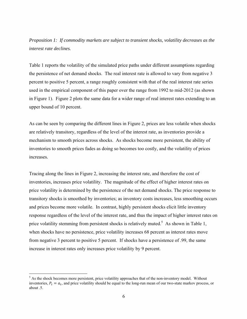
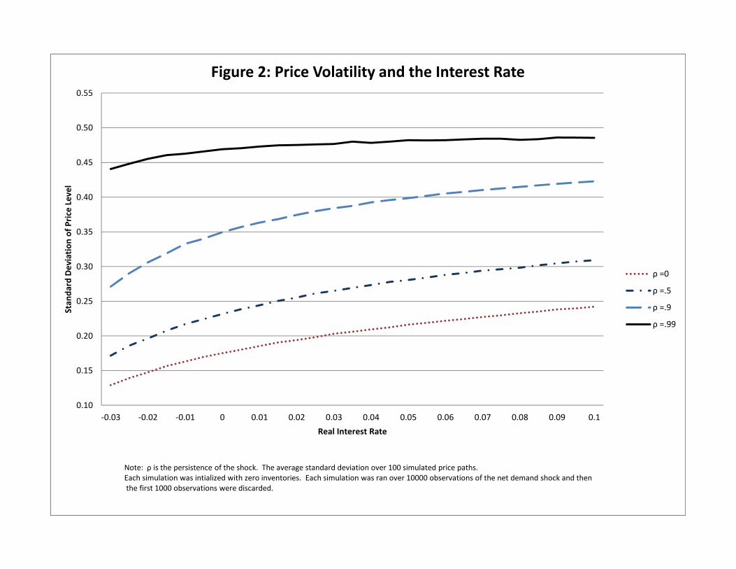
Proposition 1: If commodity markets are subject to transient shocks, volatility decreases as the

interest rate declines.

Table 1 reports the volatility of the simulated price paths under different assumptions regarding

the persistence of net demand shocks. The real interest rate is allowed to vary from negative 3

percent to positive 5 percent, a range roughly consistent with that of the real interest rate series

used in the empirical component of this paper over the range from 1992 to mid-2012 (as shown

in Figure 1). Figure 2 plots the same data for a wider range of real interest rates extending to an

upper bound of 10 percent.

As can be seen by comparing the different lines in Figure 2, prices are less volatile when shocks

are relatively transitory, regardless of the level of the interest rate, as inventories provide a

mechanism to smooth prices across shocks. As shocks become more persistent, the ability of

inventories to smooth prices fades as doing so becomes too costly, and the volatility of prices

increases.

Tracing along the lines in Figure 2, increasing the interest rate, and therefore the cost of

inventories, increases price volatility. The magnitude of the effect of higher interest rates on

price volatility is determined by the persistence of the net demand shocks. The price response to

transitory shocks is smoothed by inventories; as inventory costs increases, less smoothing occurs

and prices become more volatile. In contrast, highly persistent shocks elicit little inventory

response regardless of the level of the interest rate, and thus the impact of higher interest rates on

price volatility stemming from persistent shocks is relatively muted.5 As shown in Table 1,

when shocks have no persistence, price volatility increases 68 percent as interest rates move

from negative 3 percent to positive 5 percent. If shocks have a persistence of .99, the same

increase in interest rates only increases price volatility by 9 percent.

5 As the shock becomes more persistent, price volatility approaches that of the non-inventory model. Without inventories, , and price volatility should be equal to the long-run mean of our two-state markov process, or about .5.

7

Two Commodities

In this section we expand the model to include a second commodity. Each commodity is subject

to two shocks, an idiosyncratic shock (a) unique to an individual commodity and a common

shock (b) the affects all commodities equally. The shocks are assumed to be independent. Both

shocks are modeled as two state Markov processes a = b = {0.001,1}. The transition matrices

are identical for each of the idiosyncratic shocks, but are allowed to vary over the idiosyncratic

and the common shocks.

The model is solved in the same manner as with the single commodity model except the price

function is now defined as:

∆

The two Markov processes are combined into an irreducible four-state process and the policy

function becomes: , , . The solution to the policy function is identical across

both commodities.

To simulate price and inventory paths for both commodities, three independent Markov

processes are simulated. One process was deemed the common shock and entered into the policy

function for both commodities, while each of the remaining two shocks were construed as an

idiosyncratic shock particular to one of the two commodities.

Proposition 2: If idiosyncratic shocks are more transient than common shocks, then commodity

correlation increases as the interest rate declines.

Table 2 and Exhibit 3 examine price correlation as a function of the interest rate under different

assumptions regarding the relative persistence of common and idiosyncratic shocks. When the

common shock is relatively more persistent, price correlation is decreasing as the interest rate

increases. Conversely, if idiosyncratic shocks are more persistent than the common shock, the

correlation is increasing with the interest rate.

8

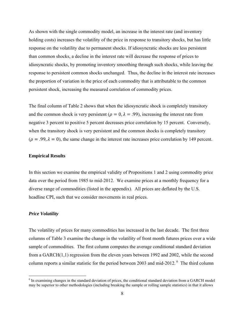
As shown with the single commodity model, an increase in the interest rate (and inventory

holding costs) increases the volatility of the price in response to transitory shocks, but has little

response on the volatility due to permanent shocks. If idiosyncratic shocks are less persistent

than common shocks, a decline in the interest rate will decrease the response of prices to

idiosyncratic shocks, by promoting inventory smoothing through such shocks, while leaving the

response to persistent common shocks unchanged. Thus, the decline in the interest rate increases

the proportion of variation in the price of each commodity that is attributable to the common

persistent shock, increasing the measured correlation of commodity prices.

The final column of Table 2 shows that when the idiosyncratic shock is completely transitory

and the common shock is very persistent ( 0, .99), increasing the interest rate from

negative 3 percent to positive 5 percent decreases price correlation by 15 percent. Conversely,

when the transitory shock is very persistent and the common shocks is completely transitory

( .99, 0), the same change in the interest rate increases price correlation by 149 percent.

Empirical Results

In this section we examine the empirical validity of Propositions 1 and 2 using commodity price

data over the period from 1985 to mid-2012. We examine prices at a monthly frequency for a

diverse range of commodities (listed in the appendix). All prices are deflated by the U.S.

headline CPI, such that we consider movements in real prices.

Price Volatility

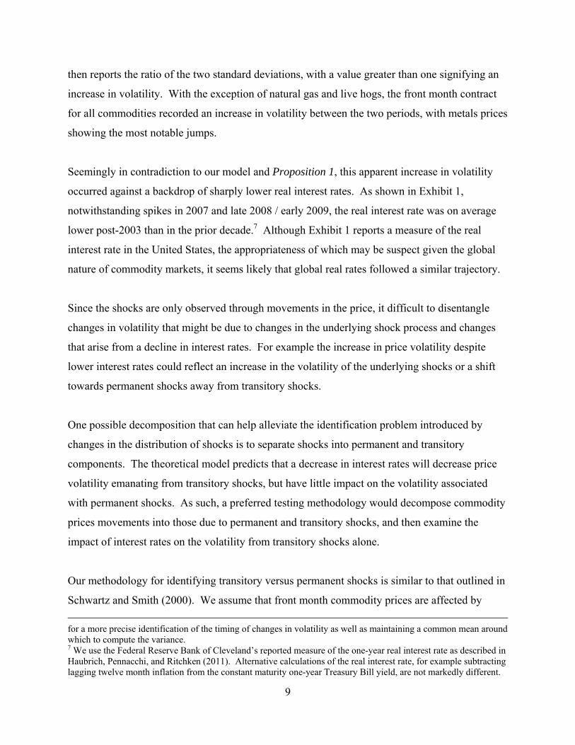
The volatility of prices for many commodities has increased in the last decade. The first three

columns of Table 3 examine the change in the volatility of front month futures prices over a wide

sample of commodities. The first column computes the average conditional standard deviation

from a GARCH(1,1) regression from the eleven years between 1992 and 2002, while the second

column reports a similar statistic for the period between 2003 and mid-2012. 6 The third column

6 In examining changes in the standard deviation of prices, the conditional standard deviation from a GARCH model may be superior to other methodologies (including breaking the sample or rolling sample statistics) in that it allows

9

then reports the ratio of the two standard deviations, with a value greater than one signifying an

increase in volatility. With the exception of natural gas and live hogs, the front month contract

for all commodities recorded an increase in volatility between the two periods, with metals prices

showing the most notable jumps.

Seemingly in contradiction to our model and Proposition 1, this apparent increase in volatility

occurred against a backdrop of sharply lower real interest rates. As shown in Exhibit 1,

notwithstanding spikes in 2007 and late 2008 / early 2009, the real interest rate was on average

lower post-2003 than in the prior decade.7 Although Exhibit 1 reports a measure of the real

interest rate in the United States, the appropriateness of which may be suspect given the global

nature of commodity markets, it seems likely that global real rates followed a similar trajectory.

Since the shocks are only observed through movements in the price, it difficult to disentangle

changes in volatility that might be due to changes in the underlying shock process and changes

that arise from a decline in interest rates. For example the increase in price volatility despite

lower interest rates could reflect an increase in the volatility of the underlying shocks or a shift

towards permanent shocks away from transitory shocks.

One possible decomposition that can help alleviate the identification problem introduced by

changes in the distribution of shocks is to separate shocks into permanent and transitory

components. The theoretical model predicts that a decrease in interest rates will decrease price

volatility emanating from transitory shocks, but have little impact on the volatility associated

with permanent shocks. As such, a preferred testing methodology would decompose commodity

prices movements into those due to permanent and transitory shocks, and then examine the

impact of interest rates on the volatility from transitory shocks alone.

Our methodology for identifying transitory versus permanent shocks is similar to that outlined in

Schwartz and Smith (2000). We assume that front month commodity prices are affected by

for a more precise identification of the timing of changes in volatility as well as maintaining a common mean around which to compute the variance. 7 We use the Federal Reserve Bank of Cleveland’s reported measure of the one-year real interest rate as described in Haubrich, Pennacchi, and Ritchken (2011). Alternative calculations of the real interest rate, for example subtracting lagging twelve month inflation from the constant maturity one-year Treasury Bill yield, are not markedly different.

10

transitory and permanent shocks, while year-ahead prices only reflect permanent shocks. Under

these assumptions movements in the time spread of the futures curve can be attributed to

transitory shocks. Testing our model then relates to examining the volatility of commodity time

spreads relative to the level of the interest rate.

Before formally examining the relationship between interest rates and price volatility, we first

compare the volatility of permanent and transitory shocks across the 1992 - 2002 and 2003 -

mid-2012 subsamples discussed earlier. As shown in columns 4 and 5 in Exhibit 3, year-ahead

futures prices are generally less volatile than the front month futures, columns 1 and 2.

However, as shown in column 6, there was a large increase in the volatility of year-ahead futures

prices post-2003, with the volatility of year-ahead crude oil contracts increasing over 80 percent

in the 2003 to 2012 period relative to the 1992 to 2002 period. In contrast, as shown in column

9, the volatility of the time spread declined in the latter period. Thus it appears as through for

most commodities the increase in the volatility of front-month contracts (shown in column 3) is

more than fully explained by an increase in the volatility of permanent shocks, while the

volatility of transitory shocks actually declined.

Next we estimate the following GARCH (1,1) model for each individual commodity,

∆ log

∗ ∗ ∗

where is a constant and is the real interest rate. Testing our model is equivalent to testing

whether d > 0, such that an increase in the interest rate increases the volatility of prices.

Our estimation results are reported in Table 4, with column 1 showing results for the front-month

contract, column 3, for the year-ahead contract (permanent shock), and column 5 for the time

spread (transitory shock). For the year-ahead contracts, the coefficient on the real interest rate is

largely insignificant, such that the interest rate appears to have no effect on the volatility of

prices in response to permanent shocks. The coefficients for the front-month contracts are also

11

insignificant, perhaps reflecting the relative importance of permanent shocks in explaining

movements in front-month prices. However, for many commodities the coefficient are

significant and positive in regard to the volatility of the time spread (column 5). This pattern of

significance and insignificance aligns with the predictions of the model, in that interest rates

should impact the response to transitory and not permanent shocks.

The model tends to work better for energy commodities and the metals and not as well for

agricultural commodities, where the coefficients in column 5 are insignificant and often of the

wrong sign. A potential explanation for this lack of significance is that physical inventory costs

tend to be higher for these commodities compared with energy and metals, as such a given

decline in the financial cost of inventories is less meaningful and less likely to have any effect on

price dynamics.

Price Correlation

The higher level and increased volatility of commodity prices over the last decade has also been

associated with an increase in commodity price correlation. Table 5 reports the difference in

pairwise correlations over the 2003 to 2012 period compared to correlation over the 1992 to

2002. A positive number reports an increase in correlation. Similar to what was reported for

volatility, the correlation was calculated as the average conditional correlation as estimated by a

panel GARCH (1,1) model over the entire sample period. As can be seen in the table, the

majority (80 percent) of pairwise correlations increased in the latter period.

As discussed in the model component of the paper, the theoretical effect of interest rates on the

correlation of commodity prices is dependent on the structure of shocks hitting commodity

markets, in particular on the relative persistence of common versus idiosyncratic shocks. It is

only when idiosyncratic shocks are relatively less persistent that lower interest rates should

increase price correlation.

Are idiosyncratic shocks less persistent than common shocks? We start by addressing a slightly

different question: Are permanent shocks more correlated than transitory shocks? Table 6

12

reports the pairwise correlation of year-ahead futures prices (permanent) less the correlation of

time-spreads (transitory) computed over the entire 1992 to mid-2012 sample. A positive number

indicates that permanent shocks are more correlated than transitory shocks. As shown in the

table, for about 75 percent of commodity pairs, year-ahead futures prices were more correlated

than time spreads.

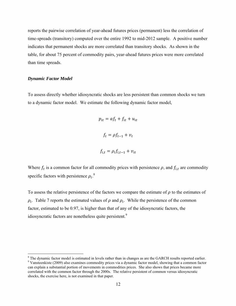
Dynamic Factor Model

To assess directly whether idiosyncratic shocks are less persistent than common shocks we turn

to a dynamic factor model. We estimate the following dynamic factor model,

, ,

Where is a common factor for all commodity prices with persistence , and , are commodity

specific factors with persistence .8

To assess the relative persistence of the factors we compare the estimate of to the estimates of

. Table 7 reports the estimated values of and . While the persistence of the common

factor, estimated to be 0.97, is higher than that of any of the idiosyncratic factors, the

idiosyncratic factors are nonetheless quite persistent.9

8 The dynamic factor model is estimated in levels rather than in changes as are the GARCH results reported earlier. 9 Vansteenkiste (2009) also examines commodity prices via a dynamic factor model, showing that a common factor can explain a substantial portion of movements in commodities prices. She also shows that prices became more correlated with the common factor through the 2000s. The relative persistent of common versus idiosyncratic shocks, the exercise here, is not examined in that paper.

13

Panel GARCH

Similar to our earlier test for the effect of the interest rate on volatility, we now estimate a panel

GARCH model to examine the impact of the interest rate on price correlation. The model is set

up as follows:

∆ log

∗ ∗ ∗

∗ ∗ ∗ ∗

In particular we our interested in examining the coefficient on the interest rate in the covariance

equations and testing whether < 0. A negative and significant coefficient indicates that

commodity correlation increases as the interest rate declines.

Rather the running the regression with the entire panel of 16 commodities in our sample, we

chose to estimate a separate two commodity panel for each of the 120 possible commodity

pairings. Using the entire panel of commodities requires estimating 560 parameters with 3920

observations, whereas with two commodities the number of coefficients is cut to 14, which in

turn are estimated over 490 observations.

Table 8 reports the coefficient estimates for as well as the associated standard errors. The

majority of the coefficients are negative, but insignificant. A potential explanation for this

insignificance could be the high persistence of idiosyncratic shocks as identified by the dynamic

factor model. Although idiosyncratic shocks appear to be less persistent than common shocks,

the difference may not be such as to result in a notable decline in price correlation as inventory

costs decline.

14

Conclusion

We examine the effect of interest rates on the volatility and correlation of commodity prices. An

established literature posits that lower interest rates raise the level of commodity prices by

lowering inventory carrying costs and increasing inventory demand. Using the framework of

Deaton and Laroque (1992) we show that lower interest rates should also decrease the volatility

of commodity prices, as lower inventory carrying costs increase incentives to smooth prices over

time in response to transient shocks. Also, we show that lower interest rates could lead to an

increase in commodity price correlation under the additional assumption that shocks common to

all commodities are more persistent than idiosyncratic shocks. With relatively more transient

idiosyncratic shocks, lower interest rates decrease the volatility of prices due to idiosyncratic

shocks but have little effect on the volatility resulting from common shocks, thereby increasing

the measured correlation of prices across commodities.

Empirically, we identify transient shocks via variation in the time spread of the futures curve,

under the assumption that persistent shocks affect both front-month and year-ahead futures

prices, while transient shocks affect only the front-month price. Using a GARCH model we

show that for a number of commodities, the volatility of the time spread falls as the real interest

rate declines, in line with the theoretical model. Examining a panel of commodity prices, we

then disentangle common versus idiosyncratic shocks via a dynamic factor model. We find that

common shocks are in fact more persistent than idiosyncratic shocks for a large number of

commodities. Using a GARCH model, we show that as the interest rate increases, the average

conditional covariance across commodity prices is decreasing; however, the coefficients are

largely insignificant. One possible explanation for the insignificance of the interest rate in

explaining changes in price correlation is the strong persistence of idiosyncratic shocks. With

both common and idiosyncratic shocks exhibiting persistence, inventory costs are relatively

unimportant for explaining

15

Bibliography

Akram, Q. Farooq, 2009, Commodity Prices, Interest Rates and the Dollar, Energy Economics

31, 838-851.

Arseneau, David M. and Sylvain Leduc, 2012, Commodity Price Movements in a General

Equilibrium Model of Storage, International Finance Discussion Paper 1054, Board of

Governors of the Federal Reserve.

Deaton, Angus, and Guy Laroque, 1992, On the Behavior of Commodity Prices, The Review of

Economic Studies 59, 1-23.

Deaton, Angus, and Guy Laroque, 1996, Competitive Storage and Commodity Price Dynamics,

Journal of Political Economy 104, 896-923.

Engel, Charles, and Kenneth D. West, 2005, Exchange Rates and Fundamentals, Journal of

Political Economy 113, 485-517.

Fattouh, Bassam, Lutz Kilian, and Lavan Mahadeva, 2012, The Role of Speculation in Oil

Markets: What Have We Learned So Far? Working Paper, University of Michigan.

Frankel, Jeffrey, 2008, The Effect of Monetary Policy on Real Commodity Prices, in John

Campbell, ed. Asset Prices and Monetary Policy (University of Chicago Press), 291-327.

Haubrich, Joseph G., George Pennacchi, and Peter Ritchken, 2011, Inflation Expectations, Real

Rates, and Risk Premia: Evidence from Inflation Swaps, Working paper 11-07, Federal Reserve

Bank of Cleveland.

Routledge, Bryan R., Duane J. Seppi, and Chester S. Spatt, 2000, Equilibrium Forward Curves

for Commodities, The Journal of Finance 55, 1297-1338.

16

Schwartz, Eduardo, and James E. Smith, 2000, Short-Term Variations and Long-Term Dynamics

in Commodity Prices, Management Science 46, 893-911.

Tang, Ke, and Wei Xiong, 2011, Index Investment and Financialization of Commodities,

Working paper, Princeton University.

Vansteenkiste, Isabel, 2009, How Important are Common Factors in Driving Non-Fuel

Commodity Prices? A Dynamic Factor Analysis, Working Paper 1072, European Central Bank.

‐3

‐2

‐1

0

1

2

3

4

51992 ‐ Jan

1992 ‐ Nov

1993 ‐ Sep

1994 ‐ Jul

1995 ‐ M

ay

1996 ‐ M

ar

1997 ‐ Jan

1997 ‐ Nov

1998 ‐ Sep

1999 ‐ Jul

2000 ‐ M

ay

2001 ‐ M

ar

2002 ‐ Jan

2002 ‐ Nov

2003 ‐ Sep

2004 ‐ Jul

2005 ‐ M

ay

2006 ‐ M

ar

2007 ‐ Jan

2007 ‐ Nov

2008 ‐ Sep

2009 ‐ Jul

2010 ‐ M

ay

2011 ‐ M

ar

2012 ‐ Jan

Percen

tFigure 1: One‐Year Real Interest Rate

Source:  Federal Reserve Bank of Cleveland as described in Haubrich, Pennacchi, and Ritchken (2011).

0.10

0.15

0.20

0.25

0.30

0.35

0.40

0.45

0.50

0.55

‐0.03 ‐0.02 ‐0.01 0 0.01 0.02 0.03 0.04 0.05 0.06 0.07 0.08 0.09 0.1

Stan

dard Deviatio

n of Pric

e Level

Real Interest Rate

Figure 2: Price Volatility and the Interest Rate

ρ =0

ρ =.5

ρ =.9

ρ =.99

Note:  ρ is the persistence of the shock.  The average standard deviation over 100 simulated price paths.  Each simulation was intialized with zero inventories.  Each simulation was ran over 10000 observations of the net demand shock and thenthe first 1000 observations were discarded. 

0.0

0.1

0.2

0.3

0.4

0.5

0.6

0.7

0.8

0.9

1.0

‐0.03 ‐0.02 ‐0.01 0 0.01 0.02 0.03 0.04 0.05 0.06 0.07 0.08 0.09 0.1

Price Co

rrelation

Real Interest Rate

Figure 3: Price Correlation and Interest Rates

ρ =0, λ =0

ρ =0, λ =.5

ρ =0, λ =.9

ρ =0, λ =.99

ρ =.5, λ =0

ρ =.9, λ =0

ρ =.99, λ =0

Note:  ρ is the persistence of the idiosyncatic shock.  λ is the persistence of the common shock.  The average correlation over 100 simulated price paths. Each simulation was intialized with zero inventories.  Each simulation was ran over 10000 observations of the net demand shock and then the first 1000observations were discarded. 

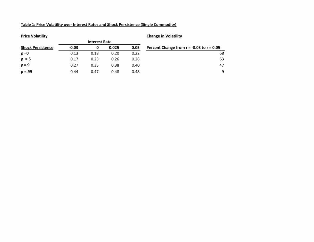
Table 1: Price Volatility over Interest Rates and Shock Persistence (Single Commodity)

Price Volatility Change in Volatility

Shock Persistence ‐0.03 0 0.025 0.05 Percent Change from r = ‐0.03 to r = 0.05ρ =0 0.13 0.18 0.20 0.22 68

ρ  =.5 0.17 0.23 0.26 0.28 63

ρ =.9 0.27 0.35 0.38 0.40 47

ρ =.99 0.44 0.47 0.48 0.48 9

Interest Rate

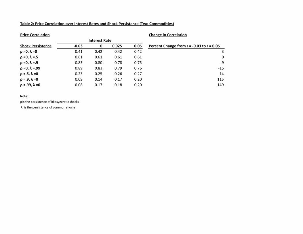
Table 2: Price Correlation over Interest Rates and Shock Persistence (Two Commodities)

Price Correlation Change in Correlation

Shock Persistence ‐0.03 0 0.025 0.05 Percent Change from r = ‐0.03 to r = 0.05ρ =0, λ =0 0.41 0.42 0.42 0.42 3

ρ =0, λ =.5 0.61 0.61 0.61 0.61 0

ρ =0, λ =.9 0.83 0.80 0.78 0.75 ‐9

ρ =0, λ =.99 0.89 0.83 0.79 0.76 ‐15

ρ =.5, λ =0 0.23 0.25 0.26 0.27 14

ρ =.9, λ =0 0.09 0.14 0.17 0.20 115

ρ =.99, λ =0 0.08 0.17 0.18 0.20 149

Note:

ρ is the persistence of idiosyncratic shocks

 λ  is the persistence of common shocks.

Interest Rate

Table 3: Commodity Price VolatilityStandard Deviation of Log Changes

1 2 3 4 5 6 7 8 9

1992:1 to 2002:12

2003:1 to 2012:7 Ratio

1992:1 to 2002:12

2003:1 to 2012:7 Ratio

1992:1 to 2002:12

2003:1 to 2012:7 Ratio

EnergyCrude Oil 0.073 0.082 1.123 0.037 0.068 1.843 0.047 0.041 0.886

Heating Oil 0.070 0.080 1.147 0.036 0.063 1.761 0.045 0.039 0.851

Natural Gas 0.089 0.125 1.402 0.057 0.061 1.077 0.089 0.089 1.000

Raw MaterialsCotton 0.066 0.083 1.245 0.039 0.055 1.409 0.040 0.047 1.181

Foods & BeveragesCocoa 0.064 0.065 1.015 0.054 0.058 1.075 0.019 0.018 0.911Corn 0.063 0.070 1.124 0.039 0.053 1.361 0.032 0.031 0.958

Live Hogs 0.077 0.071 0.931 0.046 0.044 0.951 0.082 0.074 0.905

Orange Juice 0.067 0.072 1.072 0.052 0.051 0.975 0.029 0.029 0.985

Soybeans 0.053 0.064 1.208 0.045 0.051 1.118 0.028 0.037 1.308

Soybean Meal 0.058 0.073 1.244 0.048 0.055 1.142 0.039 0.045 1.151

Soybean Oil 0.054 0.060 1.110 0.048 0.054 1.126 0.016 0.016 1.002

Wheat 0.062 0.074 1.191 0.042 0.053 1.254 0.037 0.041 1.116

MetalsAluminum 0.043 0.054 1.264 0.030 0.048 1.617 0.022 0.018 0.835

Copper 0.062 0.073 1.168 0.047 0.081 1.728 0.030 0.022 0.744

Nickel  0.070 0.099 1.414 0.061 0.083 1.355 0.021 0.039 1.864

Zinc 0.054 0.079 1.463 0.030 0.070 2.359 0.036 0.021 0.599

Note:  For the Aluminum, Copper, Nickel, and Zinc, year‐ahead futures price is the 15‐month contract.

Computed as the average conditional standard deviation from a GARCH(1,1) model.

Front Month Price Year Ahead Futures Price Time Spread (Ft/St)

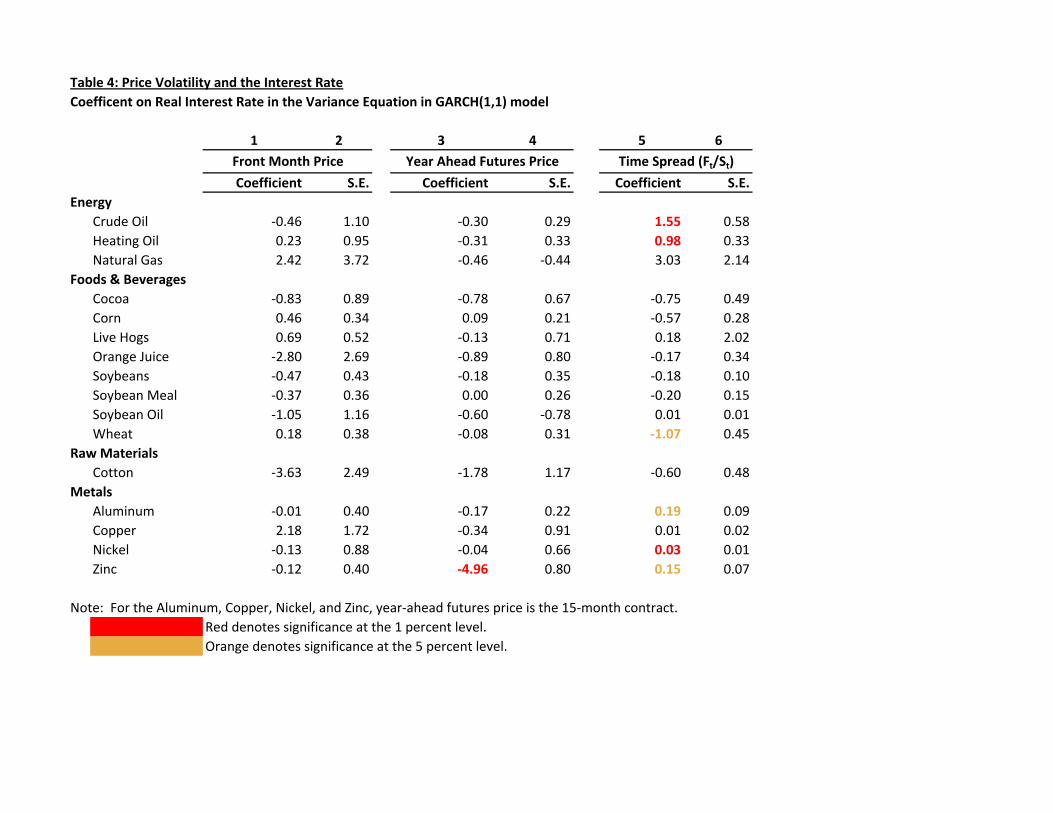
Table 4: Price Volatility and the Interest RateCoefficent on Real Interest Rate in the Variance Equation in GARCH(1,1) model

1 2 3 4 5 6

Coefficient S.E. Coefficient S.E. Coefficient S.E.Energy

Crude Oil ‐0.46 1.10 ‐0.30 0.29 1.55 0.58

Heating Oil 0.23 0.95 ‐0.31 0.33 0.98 0.33

Natural Gas 2.42 3.72 ‐0.46 ‐0.44 3.03 2.14

Foods & BeveragesCocoa ‐0.83 0.89 ‐0.78 0.67 ‐0.75 0.49

Corn 0.46 0.34 0.09 0.21 ‐0.57 0.28

Live Hogs 0.69 0.52 ‐0.13 0.71 0.18 2.02

Orange Juice ‐2.80 2.69 ‐0.89 0.80 ‐0.17 0.34

Soybeans ‐0.47 0.43 ‐0.18 0.35 ‐0.18 0.10

Soybean Meal ‐0.37 0.36 0.00 0.26 ‐0.20 0.15

Soybean Oil ‐1.05 1.16 ‐0.60 ‐0.78 0.01 0.01

Wheat 0.18 0.38 ‐0.08 0.31 ‐1.07 0.45

Raw MaterialsCotton ‐3.63 2.49 ‐1.78 1.17 ‐0.60 0.48

MetalsAluminum ‐0.01 0.40 ‐0.17 0.22 0.19 0.09

Copper 2.18 1.72 ‐0.34 0.91 0.01 0.02

Nickel  ‐0.13 0.88 ‐0.04 0.66 0.03 0.01

Zinc ‐0.12 0.40 ‐4.96 0.80 0.15 0.07

Note:  For the Aluminum, Copper, Nickel, and Zinc, year‐ahead futures price is the 15‐month contract.

Red denotes significance at the 1 percent level.

Orange denotes significance at the 5 percent level.

Front Month Price Year Ahead Futures Price Time Spread (Ft/St)

Table 5:  Commodity Price CorrelationCorrelation of Log Changes 2003:1 to 2012:7 Minus Correlation of Log Changes 1992:1 to 2002:12

Crude Heating Natural Orange Soybean SoybeanOil Oil Gas Cotton Cocoa Corn Hogs Juice Soybeans Meal Oil  Wheat Alum. Copper Nickel 

Heating Oil 0.15

Natural Gas ‐0.02 ‐0.06

Cotton 0.14 0.18 ‐0.01

Cocoa 0.17 0.40 0.11 0.13

Corn 0.09 0.19 0.23 0.02 0.15

Hogs ‐0.09 ‐0.13 0.06 ‐0.04 0.18 0.08

Orange Juice 0.12 0.13 ‐0.07 0.15 ‐0.05 0.06 0.17

Soybeans 0.17 0.30 0.07 0.20 0.16 0.23 ‐0.04 ‐0.02

Soybean Meal 0.02 0.03 ‐0.07 0.11 0.22 0.24 ‐0.04 0.01 0.25

Soybean Oil 0.43 0.36 0.09 0.33 0.18 0.24 0.09 0.03 0.37 0.62

Wheat 0.22 0.06 0.01 0.24 0.08 0.07 ‐0.04 0.07 0.19 0.27 0.11

Alum. 0.34 0.37 0.16 0.12 0.24 0.36 0.02 0.23 0.19 0.17 0.35 0.20

Copper 0.41 0.24 ‐0.14 ‐0.01 0.14 0.32 ‐0.01 0.28 0.02 0.04 0.22 0.13 ‐0.13

Nickel 0.19 0.22 0.13 0.02 0.27 0.07 ‐0.09 0.20 0.12 0.03 0.28 0.05 ‐0.09 0.21

Zinc 0.23 0.16 ‐0.02 0.05 0.11 0.29 ‐0.04 0.25 0.12 ‐0.04 0.32 0.36 0.16 0.00 ‐0.13

Note:  Front month contracts.  Average conditional correlation from panel GARCH(1,1) model.

Table 6:  Commodity Price CorrelationCorrelation of Year‐ahead Futures Prices Minus Correlation of Time Spread (Ft/St)

Crude Heating Natural Orange Soybean SoybeanOil Oil Gas Cotton Cocoa Corn Hogs Juice Soybeans Meal Oil  Wheat Alum. Copper Nickel 

Heating Oil 0.23

Natural Gas ‐0.04 ‐0.17

Cotton 0.04 0.16 ‐0.13

Cocoa 0.27 0.25 0.14 0.12

Corn 0.03 ‐0.05 ‐0.06 0.12 ‐0.08

Hogs 0.03 0.04 ‐0.08 ‐0.01 ‐0.03 0.17

Orange Juice 0.01 0.06 0.15 0.10 ‐0.09 ‐0.03 0.05

Soybeans 0.21 0.17 ‐0.01 0.20 ‐0.07 0.40 ‐0.02 0.08

Soybean Meal 0.16 0.13 0.02 0.13 ‐0.10 0.46 0.00 0.07 0.08

Soybean Oil 0.13 0.10 ‐0.04 0.24 0.04 0.25 0.03 0.07 0.41 0.29

Wheat 0.02 ‐0.06 ‐0.05 0.22 0.05 0.16 0.17 0.06 0.41 0.46 0.30

Alum. 0.09 0.08 ‐0.09 0.25 0.05 0.02 ‐0.01 0.10 0.04 0.02 0.25 0.06

Copper 0.21 0.19 ‐0.01 0.29 0.08 ‐0.03 ‐0.04 0.14 0.00 0.00 0.12 0.05 0.26

Nickel 0.18 ‐0.01 ‐0.23 0.23 ‐0.04 ‐0.02 ‐0.06 ‐0.01 0.05 0.09 0.16 0.09 0.22 0.35

Zinc 0.22 0.13 ‐0.01 0.22 0.10 0.04 0.00 ‐0.01 0.04 0.03 0.15 0.08 0.19 0.35 0.28

Note:  Average conditional correlation from panel GARCH(1,1) model for 1992:1 to 2012:7 period.

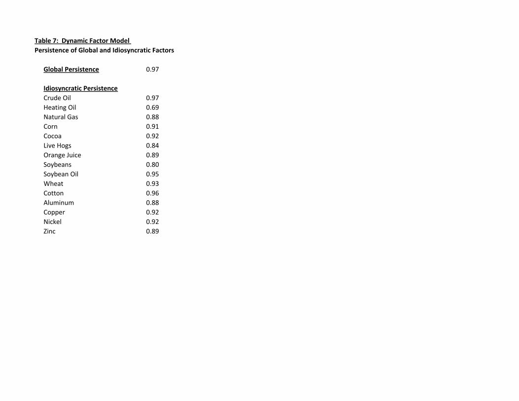
Table 7:  Dynamic Factor Model Persistence of Global and Idiosyncratic Factors

Global Persistence 0.97

Crude Oil 0.97

Heating Oil 0.69

Natural Gas    0.88

Corn 0.91

Cocoa  0.92

Live Hogs 0.84

Orange Juice 0.89

Soybeans 0.80

Soybean Oil 0.95

Wheat 0.93

Cotton 0.96

Aluminum 0.88

Copper 0.92

Nickel 0.92

Zinc 0.89

Idiosyncratic Persistence

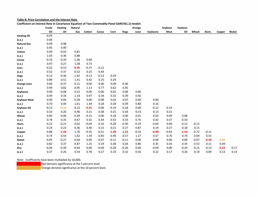
Table 8: Price Correlation and the Interest Rate  Coefficient on Interest Rate in Covariance Equation of Two‐Commodity Panel GARCH(1,1) models

Crude Heating Natural Orange Soybean SoybeanOil Oil Gas Cotton Cocoa Corn Hogs Juice Soybeans Meal Oil Wheat Alum. Copper Nickel 

Heating Oil ‐0.03

(s.e.) 0.06

Natural Gas ‐0.09 0.98

(s.e.) 0.95 0.99

Cotton 0.00 ‐0.03 0.81

(s.e.) 1.03 0.36 0.88

Cocoa ‐0.33 ‐0.34 ‐1.36 0.00

(s.e.) 0.97 0.27 1.28 0.73

Corn ‐0.32 ‐0.53 0.95 ‐0.37 ‐0.12

(s.e.) 0.52 0.37 0.52 0.25 0.44

Hogs ‐0.13 ‐0.46 ‐1.62 ‐0.13 ‐0.13 0.29

(s.e.) 0.89 0.51 1.41 0.42 0.25 0.29

Orange Juice 0.00 ‐0.37 0.11 0.00 0.00 0.09 ‐0.46

(s.e.) 0.99 0.82 0.95 1.13 0.77 0.62 0.45

Soybeans 0.00 ‐0.08 0.22 0.00 0.00 0.02 0.08 0.00

(s.e.) 0.49 0.34 1.14 0.97 0.34 0.32 0.39 0.56

Soybean Meal 0.00 0.04 0.28 0.00 ‐0.08 0.03 0.07 0.00 0.00

(s.e.) 0.70 0.44 1.61 1.34 0.18 0.28 0.39 0.80 0.16

Soybean Oil ‐0.13 ‐0.44 0.22 ‐0.41 0.00 ‐0.19 0.18 0.00 ‐0.12 ‐0.19

(s.e.) 0.33 0.26 0.96 0.21 0.38 0.25 0.44 0.53 0.13 0.21

Wheat 0.00 ‐0.06 0.49 ‐0.15 0.00 0.18 0.00 0.01 0.03 0.09 0.08

(s.e.) 0.78 0.35 0.67 0.32 0.44 0.53 0.33 0.75 0.42 0.37 0.50

Alum. ‐0.22 ‐0.21 0.02 ‐0.04 ‐0.16 ‐0.28 ‐0.30 ‐0.19 ‐0.04 0.00 ‐0.12 ‐0.12

(s.e.) 0.24 0.23 0.36 0.40 0.15 0.21 0.27 0.87 0.19 0.27 0.18 0.15

Copper ‐0.88 ‐1.44 1.70 ‐0.35 ‐0.51 ‐1.38 1.23 ‐0.54 ‐0.90 ‐0.63 ‐1.54 ‐0.72 ‐0.11

(s.e.) 0.74 0.54 1.62 1.34 0.83 0.49 0.57 1.17 0.57 0.70 0.70 0.69 0.55

Nickel ‐0.05 ‐0.27 0.04 0.00 ‐0.07 ‐0.12 ‐0.11 0.00 0.00 0.00 0.00 ‐0.07 ‐0.50 ‐0.84(s.e.) 0.82 0.37 0.87 1.25 0.19 0.38 0.34 0.86 0.35 0.34 0.35 0.53 0.11 0.49

Zinc ‐0.44 ‐0.39 ‐0.64 0.00 ‐0.09 ‐0.28 ‐0.26 0.00 ‐0.09 0.00 ‐0.29 ‐0.15 ‐0.13 ‐0.52 ‐0.17

(s.e.) 0.37 0.26 0.54 0.78 0.17 0.19 0.32 0.56 0.22 0.17 0.26 0.19 0.09 0.13 0.14

Note:  Coefficients have been multiplied by 10,000.  

Red denotes significance at the 5 percent level.

Orange denotes significance at the 10 percent level.