Embed Size (px)
Citation preview
[email protected] • MTH55_Lec-64_Fa08_sec_9-5b_Logarithmic_Eqns.ppt1
Bruce Mayer, PE Chabot College Mathematics
Bruce Mayer, PELicensed Electrical & Mechanical Engineer
Chabot Mathematics
§9.6 Exponential§9.6 ExponentialGrowth & DecayGrowth & Decay
[email protected] • MTH55_Lec-64_Fa08_sec_9-5b_Logarithmic_Eqns.ppt2
Bruce Mayer, PE Chabot College Mathematics
Review §Review §
Any QUESTIONS About• §9.5 → Exponential Equations
Any QUESTIONS About HomeWork• §9.5 → HW-47
9.5 MTH 55
[email protected] • MTH55_Lec-64_Fa08_sec_9-5b_Logarithmic_Eqns.ppt3
Bruce Mayer, PE Chabot College Mathematics
Exponential Growth or DecayExponential Growth or Decay
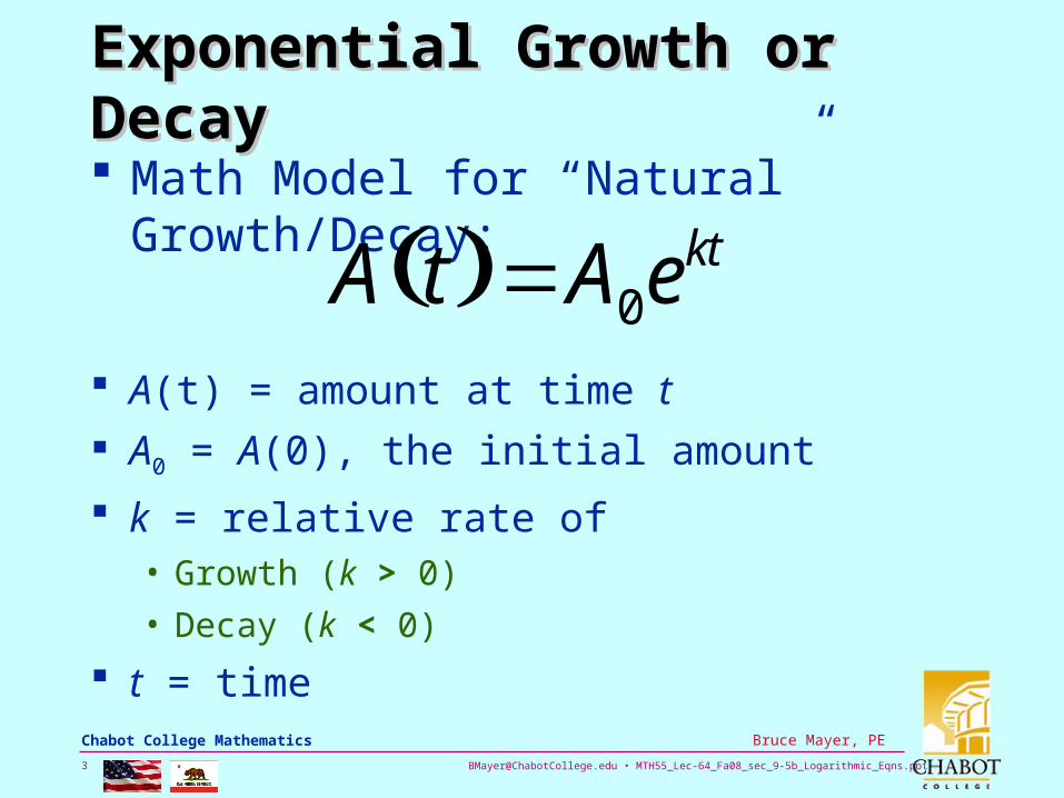
Math Model for “Natural” Growth/Decay:
A t A0ekt
A(t) = amount at time t
A0 = A(0), the initial amount
k = relative rate of • Growth (k > 0)
• Decay (k < 0)
t = time
[email protected] • MTH55_Lec-64_Fa08_sec_9-5b_Logarithmic_Eqns.ppt4
Bruce Mayer, PE Chabot College Mathematics
Exponential GrowthExponential Growth
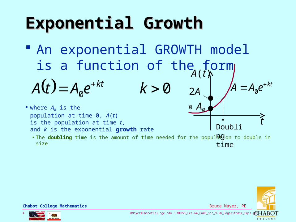
An exponential GROWTH model is a function of the form
00 keAtA kt
where A0 is the population at time 0, A(t) is the population at time t, and k is the exponential growth rate • The doubling time is the amount of time needed for the population to double in size
A0
A(t)
t
2A0
Doubling time
kteAA 0
[email protected] • MTH55_Lec-64_Fa08_sec_9-5b_Logarithmic_Eqns.ppt5
Bruce Mayer, PE Chabot College Mathematics
Exponential DecayExponential Decay
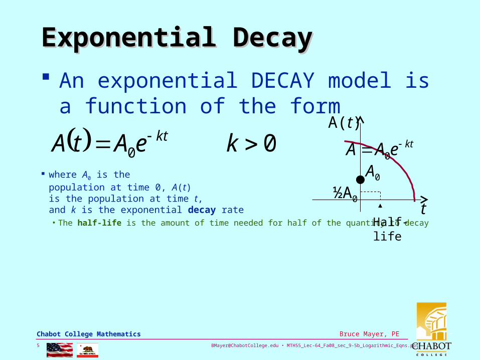
An exponential DECAY model is a function of the form
00 keAtA kt
where A0 is the population at time 0, A(t) is the population at time t, and k is the exponential decay rate • The half-life is the amount of time needed for half of the quantity to decay
A0
A(t)
t½A0
Half-life
kteAA 0
[email protected] • MTH55_Lec-64_Fa08_sec_9-5b_Logarithmic_Eqns.ppt6
Bruce Mayer, PE Chabot College Mathematics
Example Example Carbon Emissions Carbon Emissions In 1995, the United States emitted
about 1400 million tons of carbon into the atmosphere. In the same year, China emitted about 850 million tons.
Suppose the annual rate of growth of the carbon emissions in the United States and China are 1.5% and 4.5%, respectively.
After how many years will China be emitting more carbon into Earth’s atmosphere than the United States?
[email protected] • MTH55_Lec-64_Fa08_sec_9-5b_Logarithmic_Eqns.ppt7
Bruce Mayer, PE Chabot College Mathematics
Example Example Carbon Emissions Carbon Emissions
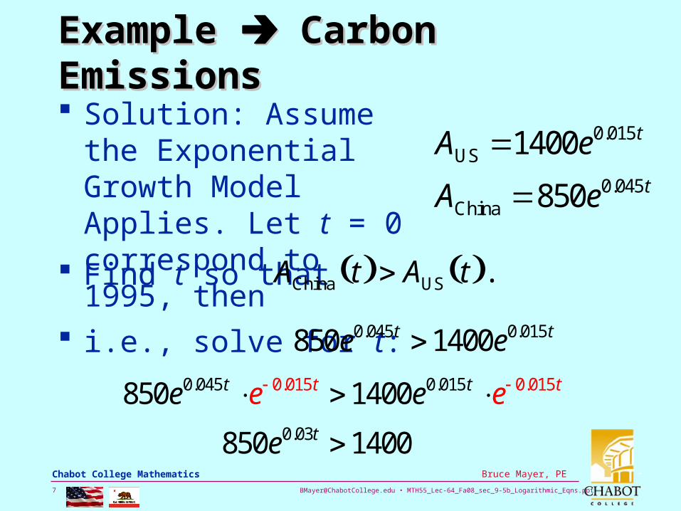
Solution: Assume the Exponential Growth Model Applies. Let t = 0 correspond to 1995, then
AUS 1400e0.015t
AChina 850e0.045t
Find t so that AChina t AUS t .
i.e., solve for t: 850e0.045t 1400e0.015t
850e0.045t e 0.015t 1400e0.015t e 0.015t
850e0.03t 1400
[email protected] • MTH55_Lec-64_Fa08_sec_9-5b_Logarithmic_Eqns.ppt8
Bruce Mayer, PE Chabot College Mathematics
Example Example Carbon Emissions Carbon Emissions
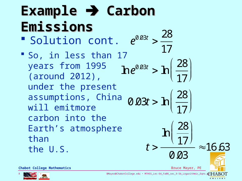
Solution cont. e0.03t 28
17
lne0.03t ln28
17
0.03t ln28
17
t ln
2817
0.0316.63
So, in less than 17 years from 1995 (around 2012), under the present assumptions, China will emitmore carbon into the Earth’s atmosphere than the U.S.
[email protected] • MTH55_Lec-64_Fa08_sec_9-5b_Logarithmic_Eqns.ppt9
Bruce Mayer, PE Chabot College Mathematics
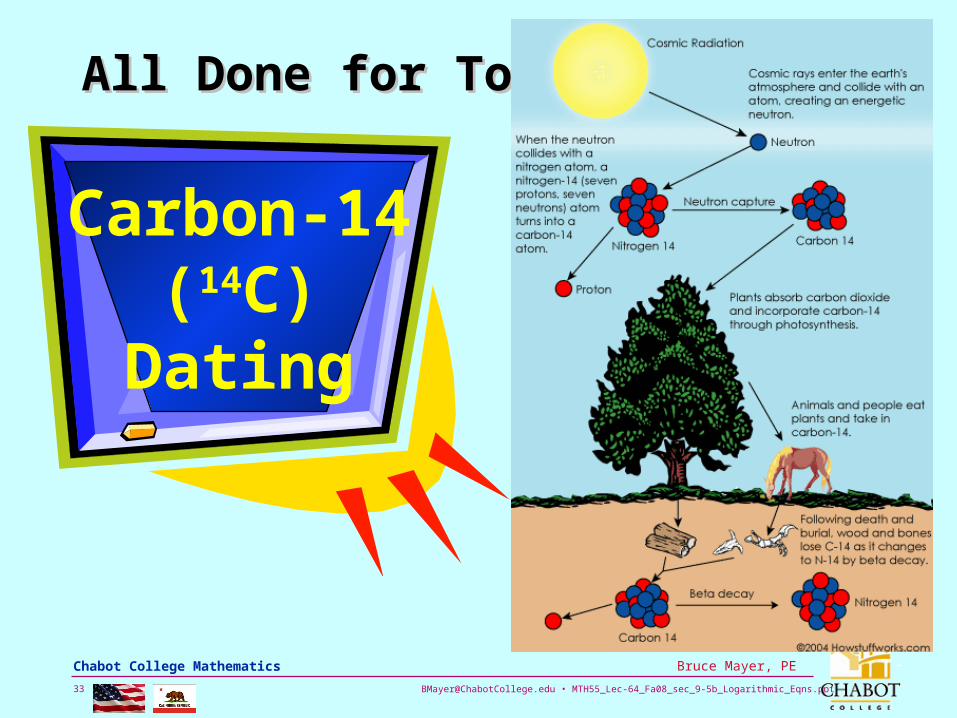
Example Example Carbon Dating Carbon Dating
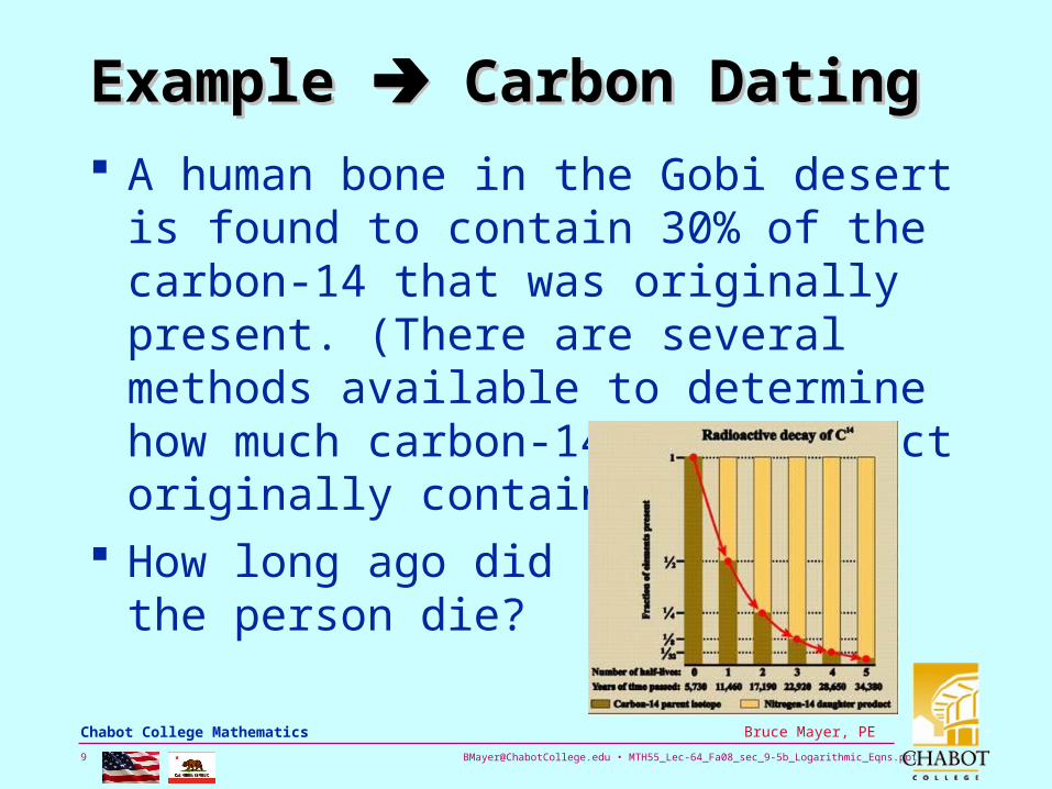
A human bone in the Gobi desert is found to contain 30% of the carbon-14 that was originally present. (There are several methods available to determine how much carbon-14 the artifact originally contained.)
How long ago didthe person die?
[email protected] • MTH55_Lec-64_Fa08_sec_9-5b_Logarithmic_Eqns.ppt10
Bruce Mayer, PE Chabot College Mathematics
Example Example Carbon Dating Carbon Dating
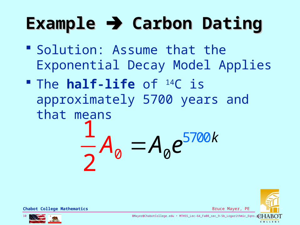
Solution: Assume that the Exponential Decay Model Applies
The half-life of 14C is approximately 5700 years and that means
1
2A0 A0e
5700k
[email protected] • MTH55_Lec-64_Fa08_sec_9-5b_Logarithmic_Eqns.ppt11
Bruce Mayer, PE Chabot College Mathematics
Example Example Carbon Dating Carbon Dating
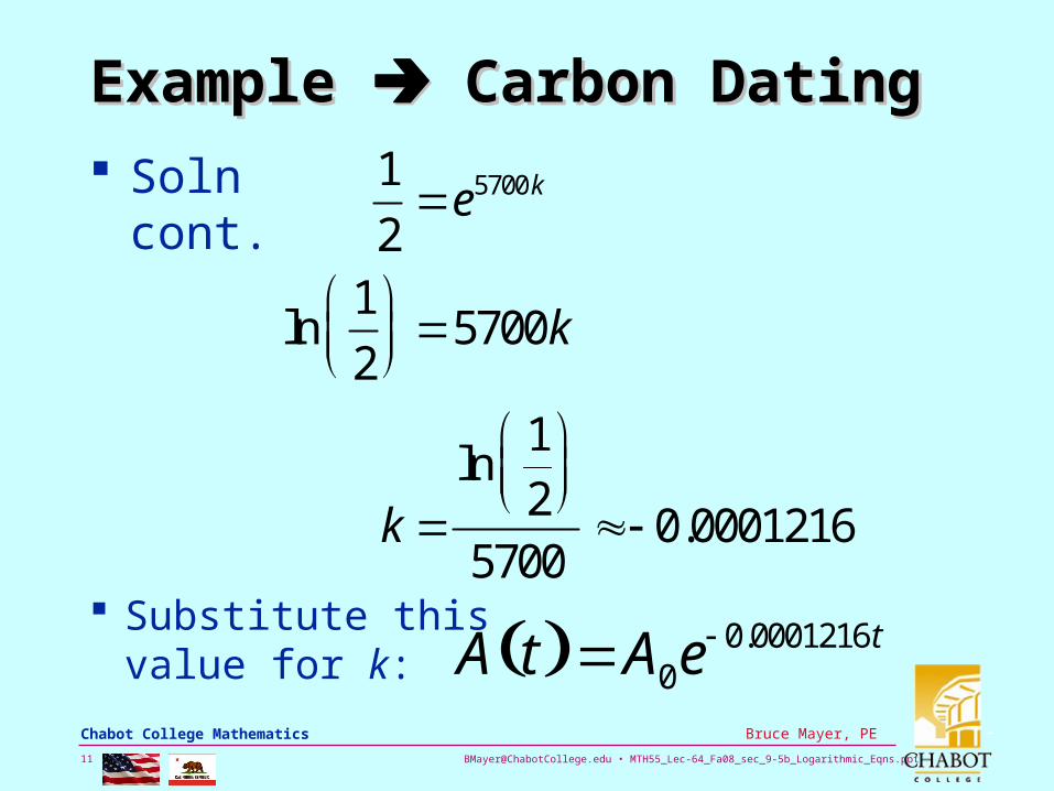
Solncont.
1
2e5700k
ln1
2
5700k
k ln
12
5700 0.0001216
Substitute this value for k: A t A0e
0.0001216t
[email protected] • MTH55_Lec-64_Fa08_sec_9-5b_Logarithmic_Eqns.ppt12
Bruce Mayer, PE Chabot College Mathematics
Example Example Carbon Dating Carbon Dating
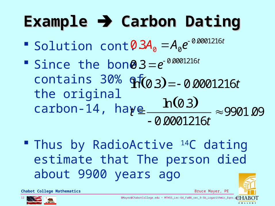
Solution cont. Since the bone
contains 30% of the original carbon-14, have
0.3A0 A0e 0.0001216t
0.3 e 0.0001216t
ln 0.3 0.0001216t
t ln 0.3
0.0001216t9901.09
Thus by RadioActive 14C dating estimate that The person died about 9900 years ago
[email protected] • MTH55_Lec-64_Fa08_sec_9-5b_Logarithmic_Eqns.ppt13
Bruce Mayer, PE Chabot College Mathematics
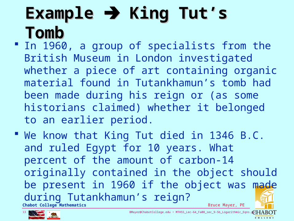
Example Example King Tut’s Tomb King Tut’s Tomb In 1960, a group of specialists from the British
Museum in London investigated whether a piece of art containing organic material found in Tutankhamun’s tomb had been made during his reign or (as some historians claimed) whether it belonged to an earlier period.
We know that King Tut died in 1346 B.C. and ruled Egypt for 10 years. What percent of the amount of carbon-14 originally contained in the object should be present in 1960 if the object was made during Tutankhamun’s reign?
[email protected] • MTH55_Lec-64_Fa08_sec_9-5b_Logarithmic_Eqns.ppt14
Bruce Mayer, PE Chabot College Mathematics
Example Example King Tut’s Tomb King Tut’s Tomb
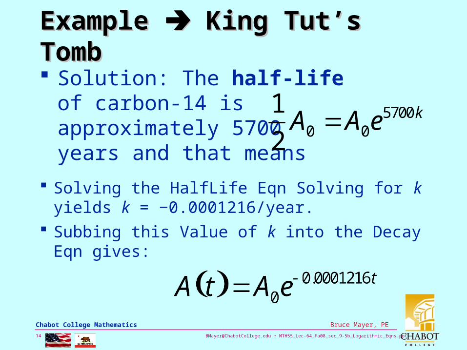
Solution: The half-life of carbon-14 is approximately 5700 years and that means
1
2A0 A0e
5700k
Solving the HalfLife Eqn Solving for k yields k = −0.0001216/year.
Subbing this Value of k into the Decay Eqn gives:
[email protected] • MTH55_Lec-64_Fa08_sec_9-5b_Logarithmic_Eqns.ppt15
Bruce Mayer, PE Chabot College Mathematics
Example Example King Tut’s Tomb King Tut’s Tomb
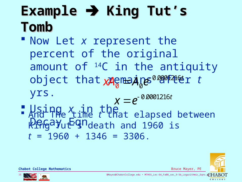
Now Let x represent the percent of the original amount of 14C in the antiquity object that remains after t yrs.
Using x in theDecay Eqn
xA0 A0e 0.0001216t
x e 0.0001216t
And The time t that elapsed between King Tut’s death and 1960 is t = 1960 + 1346 = 3306.
[email protected] • MTH55_Lec-64_Fa08_sec_9-5b_Logarithmic_Eqns.ppt16
Bruce Mayer, PE Chabot College Mathematics
Example Example King Tut’s Tomb King Tut’s Tomb
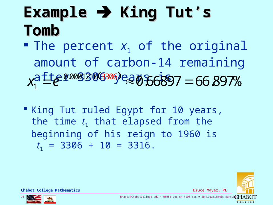
The percent x1 of the original amount of carbon-14 remaining after 3306 years is
x1 e 0.0001216 3306 0.66897 66.897%
King Tut ruled Egypt for 10 years, the time t1 that elapsed from the beginning of his reign to 1960 is t1 = 3306 + 10 = 3316.
[email protected] • MTH55_Lec-64_Fa08_sec_9-5b_Logarithmic_Eqns.ppt17
Bruce Mayer, PE Chabot College Mathematics
Example Example King Tut’s Tomb King Tut’s Tomb
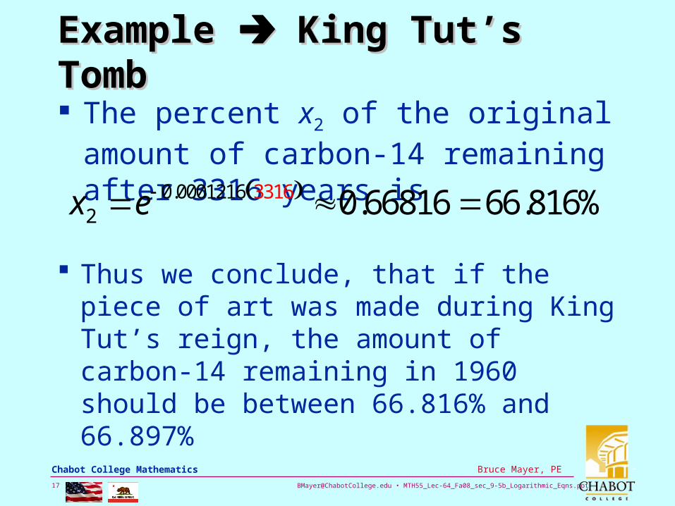
The percent x2 of the original amount of carbon-14 remaining after 3316 years is
x2 e 0.0001216 3316 0.66816 66.816%
Thus we conclude, that if the piece of art was made during King Tut’s reign, the amount of carbon-14 remaining in 1960 should be between 66.816% and 66.897%
[email protected] • MTH55_Lec-64_Fa08_sec_9-5b_Logarithmic_Eqns.ppt18
Bruce Mayer, PE Chabot College Mathematics
Newton’s Law of CoolingNewton’s Law of Cooling
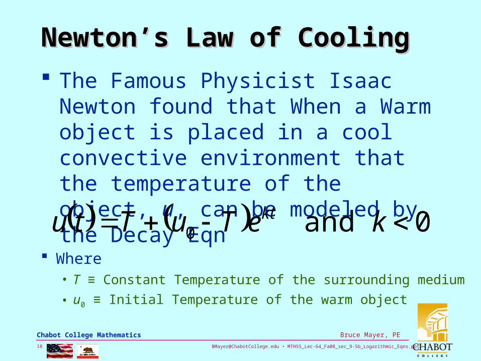
The Famous Physicist Isaac Newton found that When a Warm object is placed in a cool convective environment that the temperature of the object, u, can be modeled by the Decay Eqn
0and0 keTuTtu kt
Where• T ≡ Constant Temperature of the surrounding medium
• u0 ≡ Initial Temperature of the warm object
[email protected] • MTH55_Lec-64_Fa08_sec_9-5b_Logarithmic_Eqns.ppt19
Bruce Mayer, PE Chabot College Mathematics
Newton’s Law of CoolingNewton’s Law of Cooling
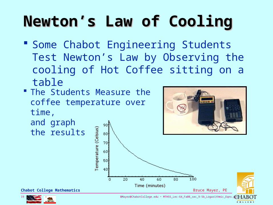
Some Chabot Engineering Students Test Newton’s Law by Observing the cooling of Hot Coffee sitting on a table
The Students Measure the coffee temperature over time, and graph the results
[email protected] • MTH55_Lec-64_Fa08_sec_9-5b_Logarithmic_Eqns.ppt20
Bruce Mayer, PE Chabot College Mathematics
Newton’s Law of CoolingNewton’s Law of Cooling
During the course of the experiment the students find• The Room Temperature, T = 21 °C
• The Initial Temperature, u0 = 93 °C
• The Water Temperature is 55 °C after 32 minutes → in Fcn notation: u0(32min)= 55 °C
Find Newton’s Cooling Law Model Equation for this situation
[email protected] • MTH55_Lec-64_Fa08_sec_9-5b_Logarithmic_Eqns.ppt21
Bruce Mayer, PE Chabot College Mathematics
Newton’s Law of CoolingNewton’s Law of Cooling
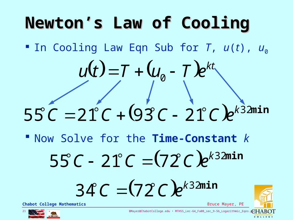
In Cooling Law Eqn Sub for T, u(t), u0
kteTuTtu 0
min3221932155 keCCCC Now Solve for the Time-Constant k
min32722155 keCCC
min327234 keCC
[email protected] • MTH55_Lec-64_Fa08_sec_9-5b_Logarithmic_Eqns.ppt22
Bruce Mayer, PE Chabot College Mathematics
Newton’s Law of CoolingNewton’s Law of Cooling
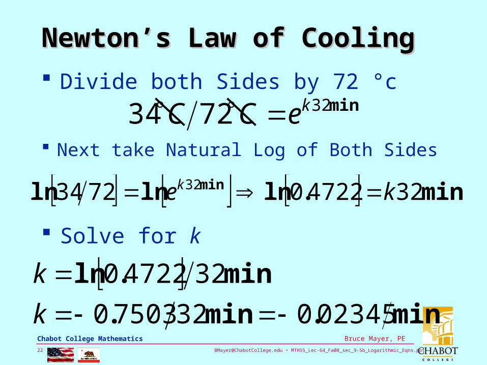
Divide both Sides by 72 °c
min.lnlnln min 32472207234 32 kek
min327234 keCC Next take Natural Log of Both Sides
Solve for k
min.min.
min.ln
0234503275030
3247220
k
k
[email protected] • MTH55_Lec-64_Fa08_sec_9-5b_Logarithmic_Eqns.ppt23
Bruce Mayer, PE Chabot College Mathematics
Newton’s Law of CoolingNewton’s Law of Cooling
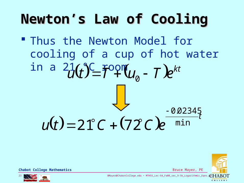
Thus the Newton Model for cooling of a cup of hot water in a 21 °C room
kteTuTtu 0
teCCtu min
02345.0
7221
[email protected] • MTH55_Lec-64_Fa08_sec_9-5b_Logarithmic_Eqns.ppt24
Bruce Mayer, PE Chabot College Mathematics
Newton’s Law of CoolingNewton’s Law of Cooling
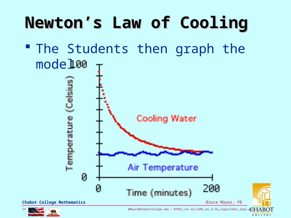
The Students then graph the model
[email protected] • MTH55_Lec-64_Fa08_sec_9-5b_Logarithmic_Eqns.ppt25
Bruce Mayer, PE Chabot College Mathematics
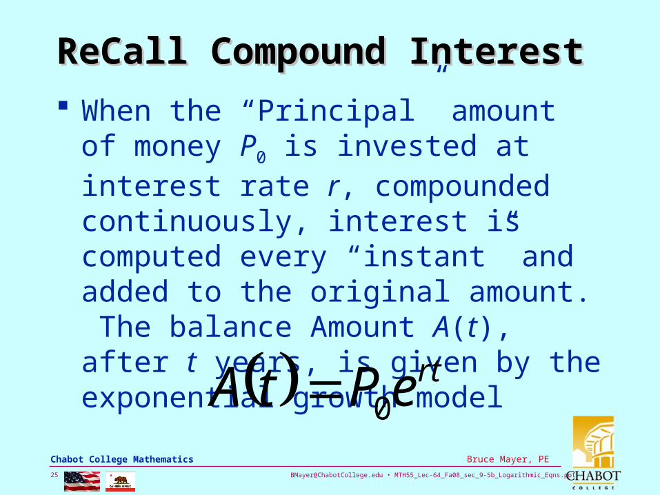
ReCall Compound InterestReCall Compound Interest
When the “Principal” amount of money P0 is invested at interest rate r, compounded continuously, interest is computed every “instant” and added to the original amount. The balance Amount A(t), after t years, is given by the exponential growth model
rtePtA 0
[email protected] • MTH55_Lec-64_Fa08_sec_9-5b_Logarithmic_Eqns.ppt26
Bruce Mayer, PE Chabot College Mathematics
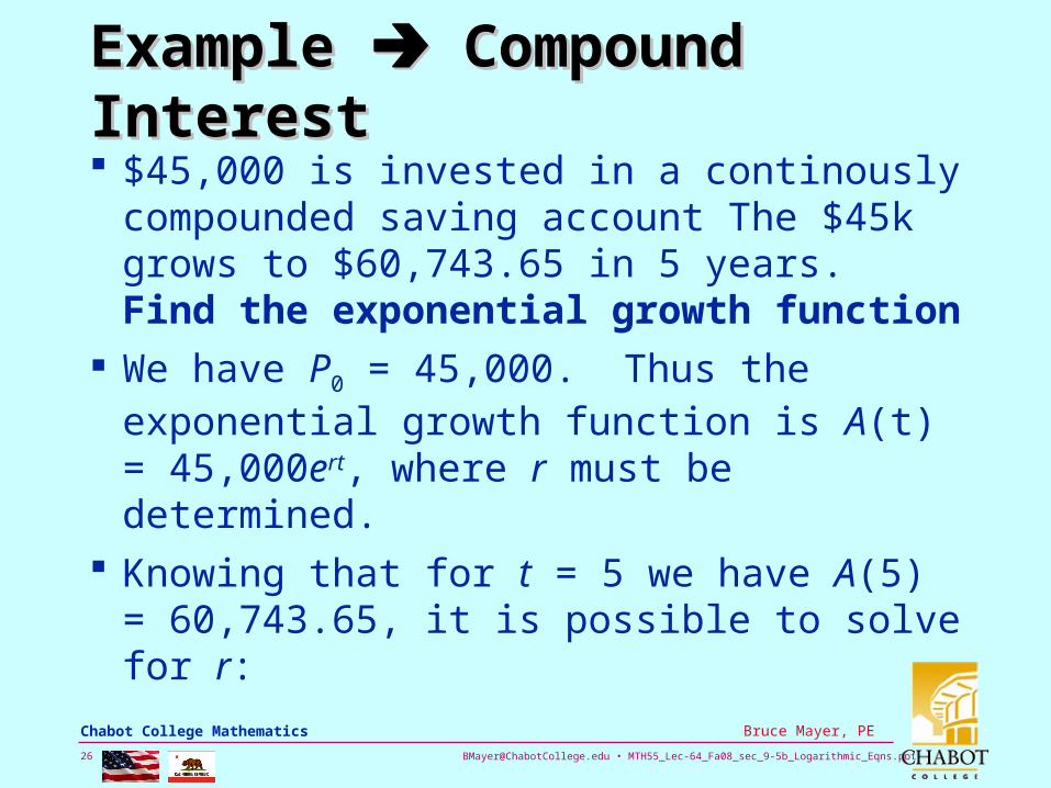
Example Example Compound Interest Compound Interest
$45,000 is invested in a continously compounded saving account The $45k grows to $60,743.65 in 5 years. Find the exponential growth function
We have P0 = 45,000. Thus the exponential growth function is A(t) = 45,000ert, where r must be determined.
Knowing that for t = 5 we have A(5) = 60,743.65, it is possible to solve for r:
[email protected] • MTH55_Lec-64_Fa08_sec_9-5b_Logarithmic_Eqns.ppt27
Bruce Mayer, PE Chabot College Mathematics
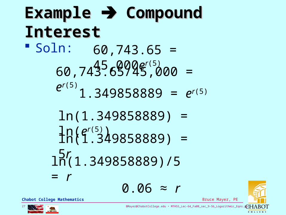
Example Example Compound Interest Compound Interest
Soln: 60,743.65 = 45,000er(5)
60,743.65/45,000 = er(5)
ln(1.349858889) = ln(er(5))
1.349858889 = er(5)
ln(1.349858889) = 5r
ln(1.349858889)/5 = r
0.06 ≈ r
[email protected] • MTH55_Lec-64_Fa08_sec_9-5b_Logarithmic_Eqns.ppt28
Bruce Mayer, PE Chabot College Mathematics
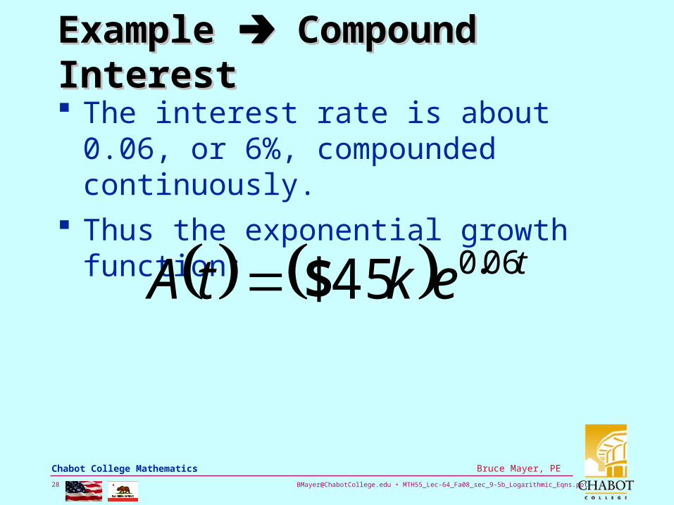
Example Example Compound Interest Compound Interest
The interest rate is about 0.06, or 6%, compounded continuously.
Thus the exponential growth function:
tektA 06045 .$
[email protected] • MTH55_Lec-64_Fa08_sec_9-5b_Logarithmic_Eqns.ppt29
Bruce Mayer, PE Chabot College Mathematics
The Logistic Growth ModelThe Logistic Growth Model
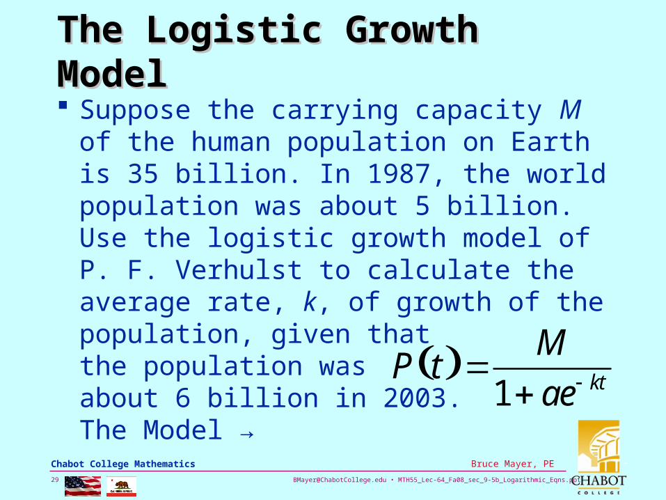
Suppose the carrying capacity M of the human population on Earth is 35 billion. In 1987, the world population was about 5 billion. Use the logistic growth model of P. F. Verhulst to calculate the average rate, k, of growth of the population, given that the population was about 6 billion in 2003. The Model →
P t M
1 ae kt
[email protected] • MTH55_Lec-64_Fa08_sec_9-5b_Logarithmic_Eqns.ppt30
Bruce Mayer, PE Chabot College Mathematics
The Logistic Growth ModelThe Logistic Growth Model
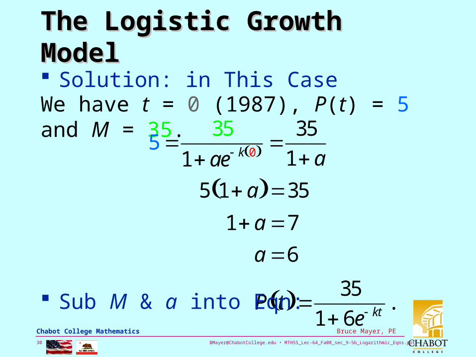
Solution: in This CaseWe have t = 0 (1987), P(t) = 5 and M = 35.
5 35
1 ae k 0 35
1 a5 1 a 35
1 a 7
a 6
P t 35
1 6e kt . Sub M & a into Eqn:
[email protected] • MTH55_Lec-64_Fa08_sec_9-5b_Logarithmic_Eqns.ppt31
Bruce Mayer, PE Chabot College Mathematics
The Logistic Growth ModelThe Logistic Growth Model
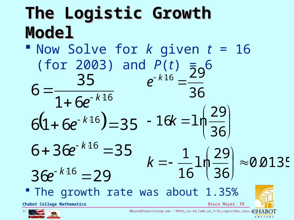
Now Solve for k given t = 16 (for 2003) and P(t) = 6
The growth rate was about 1.35%
2936
35366
35616
61
356
16
16
16
16
k
k
k
k
e
e
e
e
0135.036
29ln
16
1
36
29ln16
36
2916
k
k
e k
[email protected] • MTH55_Lec-64_Fa08_sec_9-5b_Logarithmic_Eqns.ppt32
Bruce Mayer, PE Chabot College Mathematics
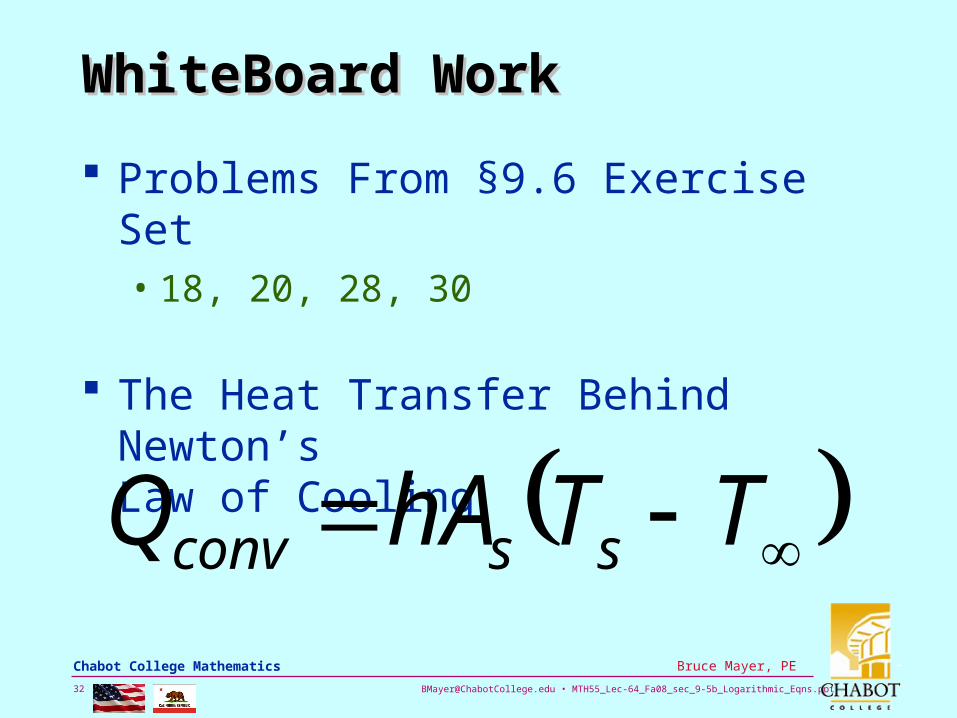
WhiteBoard WorkWhiteBoard Work
Problems From §9.6 Exercise Set• 18, 20, 28, 30
The Heat Transfer Behind Newton’sLaw of Cooling
TThAQ ssconv
[email protected] • MTH55_Lec-64_Fa08_sec_9-5b_Logarithmic_Eqns.ppt33
Bruce Mayer, PE Chabot College Mathematics
All Done for TodayAll Done for Today
Carbon-14(14C)
Dating
[email protected] • MTH55_Lec-64_Fa08_sec_9-5b_Logarithmic_Eqns.ppt34
Bruce Mayer, PE Chabot College Mathematics
Bruce Mayer, PELicensed Electrical & Mechanical Engineer
Chabot Mathematics
AppendiAppendixx
–
srsrsr 22
[email protected] • MTH55_Lec-64_Fa08_sec_9-5b_Logarithmic_Eqns.ppt35
Bruce Mayer, PE Chabot College Mathematics
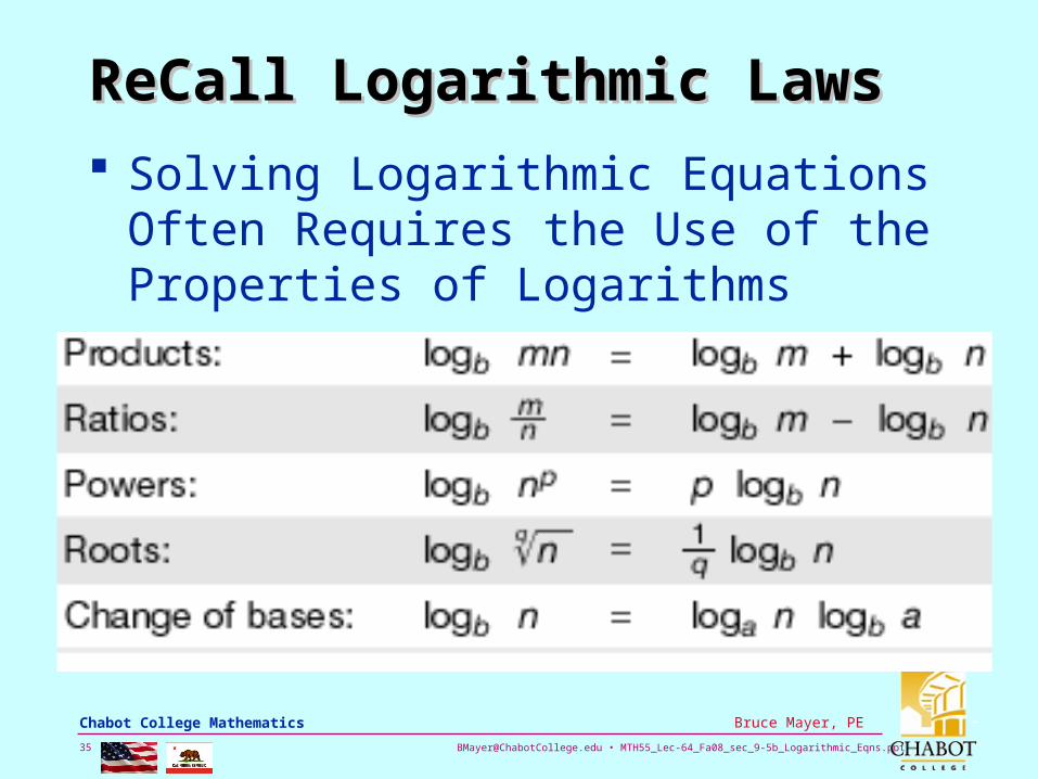
ReCall Logarithmic LawsReCall Logarithmic Laws
Solving Logarithmic Equations Often Requires the Use of the Properties of Logarithms