Bman03 Data Description

© The McGraw-Hill Companies, Inc., 2000

3-13-1

Chapter 3Chapter 3

Data DescriptionData Description


3-23-2 OutlineOutline

3-1 Introduction 3-2 Measures of Central

Tendency 3-3 Measures of Variation 3-4 Measures of Position 3-5 Exploratory Data Analysis


3-33-3 ObjectivesObjectives

Summarize data using the measures of central tendency, such as the mean, median, mode, and midrange.

Describe data using the measures of variation, such as the range, variance, and standard deviation.


3-43-4 Objectives Objectives

Identify the position of a data value in a data set using various measures of position, such as percentiles, deciles and quartiles.


3-53-5 Objectives Objectives

Use the techniques of exploratory data analysis, including stem and leaf plots, box plots, and five-number summaries to discover various aspects of data.


3-63-6 3-2 Measures of Central Tendency3-2 Measures of Central Tendency

A statisticstatistic is a characteristic or measure obtained by using the data values from a sample.

A parameterparameter is a characteristic or measure obtained by using the data values from a specific population.


3-73-7 3-2 The Mean (arithmetic average)3-2 The Mean (arithmetic average)

The meanmean is defined to be the sum of the data values divided by the total number of values.

We will compute two means: one for the sample and one for a finite population of values.


3-83-8 3-2 The Mean (arithmetic average)3-2 The Mean (arithmetic average)

The mean, in most cases, is not an actual data value.


3-93-9 3-2 The Sample Mean3-2 The Sample Mean

The symbol X represents the sample mean

X is read as X bar The Greek symbol

is read as sigma and it means to sum

XX X X

nX

n

n

.

" - ".

"

= +

" " ".

...

.

1 2


3-103-10 3-2 The Sample Mean - 3-2 The Sample Mean - Example

. 96

54 =

6

12+14+12+5+8+3 ==

.

.12 ,14 ,12 ,5 ,8 ,3

weeks

n

XX

ismeansampleThe

samplethisofageaverage

theFindand

areshelteranimalanatkittenssixof

samplerandomaofweeksinagesThe


3-113-11 3-2 The Population Mean3-2 The Population Mean

The Greek symbol represents the population

mean The symbol is read as mu

N is the size of the finite population

X X X

NX

N

N

. "

= +

".

.

...

.

1 2


3-123-12 3-2 The Population Mean3-2 The Population Mean -- Example

A small company consists of the owner the manager

the salesperson and two technicians The salaries are

listed as and

respectively Assume this is the population

Then the population mean will be

X

N

, ,

, .

$50, , , , , , , ,

. ( .)

=

= 50,000 + 20,000 + 12,000 + 9,000 + 9,000

5 =

000 20 000 12 000 9 000 9 000

$20,000.


3-133-133-2 The Sample Mean for an 3-2 The Sample Mean for an Ungrouped Frequency DistributionUngrouped Frequency Distribution

The mean for an ungrouped frequency

distributuion is given by

Xf X

nHere f is the frequency for the

corresponding value of X and n f

=( )

, = .

.


3-143-143-2 The Sample Mean for an Ungrouped 3-2 The Sample Mean for an Ungrouped Frequency Distribution - Frequency Distribution - Example

T h e s c o r e s fo r s tu d e n t s o n a p o in t

q u i z a r e g i v e n in th e ta b l e F in d th e m e a n s c o r e

.

2 5 4 .

Score, X Frequency, f

0 2

1 4

2 12

3 4

4 35

Score, X

0 2

1 4

2 12

3 4

4 35

Frequency, f


3-153-15

Score, X Frequency, f f X0 2 0

1 4 4

2 12 24

3 4 12

4 3 125

Score, X X

0 2 0

1 4 4

2 12 24

3 4 12

4 3 125

= = 5 2

2 5X

f X

n

2 0 8. .

3-2 The Sample Mean for an Ungrouped 3-2 The Sample Mean for an Ungrouped Frequency Distribution - Frequency Distribution - Example

Frequency, f f


3-163-163-2 The Sample Mean for a 3-2 The Sample Mean for a Grouped Frequency DistributionGrouped Frequency Distribution

The mean for a grouped frequency

distributu ion is given by

Xf Xn

Here X is the correspond ing

class midpoint.

m

m

=( )

.


3-173-173-2 The Sample Mean for a Grouped 3-2 The Sample Mean for a Grouped Frequency Distribution - Frequency Distribution - Example

G i v e n t h e t a b l e b e l o w f i n d t h e m e a n , .

Class Frequency, f

15.5 - 20.5 3

20.5 - 25.5 5

25.5 - 30.5 4

30.5 - 35.5 3

35.5 - 40.5 25

Class

15.5 - 20.5 3

20.5 - 25.5 5

25.5 - 30.5 4

30.5 - 35.5 3

35.5 - 40.5 25

Frequency, f


3-183-183-2 The Sample Mean for a Grouped 3-2 The Sample Mean for a Grouped Frequency Distribution - Frequency Distribution - Example

T a b l e w i t h c l a s s m i d p o i n t s Xm

, .

Class Frequency, f Xm f Xm

15.5 - 20.5 3 18 54

20.5 - 25.5 5 23 115

25.5 - 30.5 4 28 112

30.5 - 35.5 3 33 99

35.5 - 40.5 2 38 765

Class X X

15.5 - 20.5 3 18 54

20.5 - 25.5 5 23 115

25.5 - 30.5 4 28 112

30.5 - 35.5 3 33 99

35.5 - 40.5 2 38 765

Frequency, f m f m


3-193-19

=

= .

=

=

f X

and n So

Xf X

n

m

m

54 115 112 99 76

456

17

456

1726 82. .

3-2 The Sample Mean for a Grouped 3-2 The Sample Mean for a Grouped Frequency Distribution - Frequency Distribution - Example


3-203-20 3-2 The Median3-2 The Median

When a data set is ordered, it is called a data arraydata array.

The medianmedian is defined to be the midpoint of the data array.

The symbol used to denote the median is MDMD.


3-213-21 3-2 The Median - 3-2 The Median - Example

The weights (in pounds) of seven army recruits are 180, 201, 220, 191, 219, 209, and 186. Find the median.

Arrange the data in order and select the middle point.


3-223-22 3-2 The Median - 3-2 The Median - Example

Data array:Data array: 180, 186, 191, 201, 209, 219, 220.

The median, MD = 201.



In the previous example, there was an odd numberodd number of values in the data set. In this case it is easy to select the middle number in the data array.



When there is an even numbereven number of values in the data set, the median is obtained by taking the average of the two middle average of the two middle numbersnumbers.


3-253-25 3-2 The Median -3-2 The Median - Example

Six customers purchased the following number of magazines: 1, 7, 3, 2, 3, 4. Find the median.

Arrange the data in order and compute the middle point.

Data array: 1, 2, 3, 3, 4, 7. The median, MD = (3 + 3)/2 = 3.



The ages of 10 college students are: 18, 24, 20, 35, 19, 23, 26, 23, 19, 20. Find the median.

Arrange the data in order and compute the middle point.



Data array:Data array: 18, 19, 19, 20, 2020, 2323, 23, 24, 26, 35.

The median, MD = (20 + 23)/2 = MD = (20 + 23)/2 = 21.5.21.5.


3-283-283-2 The Median-Ungrouped 3-2 The Median-Ungrouped

Frequency DistributionFrequency Distribution

For an ungrouped frequency distribution, find the median by examining the cumulative frequencies to locate the middle value.


3-293-293-2 The Median-Ungrouped 3-2 The Median-Ungrouped

Frequency DistributionFrequency Distribution

If n is the sample size, compute n/2. Locate the data point where n/2 values fall below and n/2 values fall above.


3-303-303-2 The Median-Ungrouped 3-2 The Median-Ungrouped Frequency Distribution -Frequency Distribution - Example

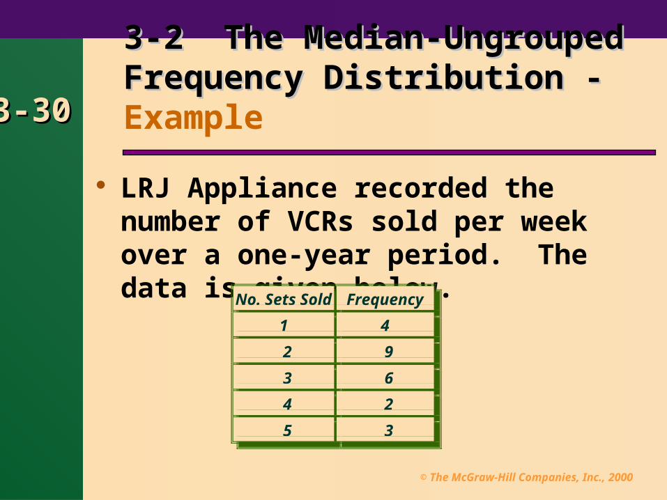
LRJ Appliance recorded the number of VCRs sold per week over a one-year period. The data is given below.

No. Sets Sold Frequency

1 4

2 9

3 6

4 2

5 3

No. Sets Sold

1 4

2 9

3 6

4 2

5 3

Frequency


3-313-313-2 The Median-Ungrouped 3-2 The Median-Ungrouped Frequency Distribution -Frequency Distribution - Example

To locate the middle point, divide n by 2; 24/2 = 12.

Locate the point where 12 values would fall below and 12 values will fall above.

Consider the cumulative distribution. The 12th and 13th values fall in class 2.

Hence MD = 2MD = 2.


3-323-32

No. Sets Sold Frequency CumulativeFrequency

1 4 4

2 9 13

3 6 19

4 2 21

5 3 24

No. Sets Sold Frequency CumulativeFrequency

1 4 4

2 9 13

3 6 19

4 2 21

5 3 24

This class contains the 5th through the 13th values.This class contains the 5th through the 13th values.

3-2 The Median-Ungrouped 3-2 The Median-Ungrouped Frequency Distribution -Frequency Distribution - Example


3-333-333-2 The Median for a Grouped 3-2 The Median for a Grouped Frequency Distribution Frequency Distribution

classmediantheofboundarylowerL

classmediantheofwidthw

classmediantheoffrequencyf

classmediantheprecedingimmediately

classtheoffrequencycumulativecf

frequenciestheofsumn

Where

Lwf

cfnMD

can be computed from:medianThe

m

m

)()2(


3-343-343-2 The Median for a Grouped 3-2 The Median for a Grouped Frequency Distribution - Frequency Distribution - Example

G i v e n t h e t a b l e b e l o w f i n d t h e m e d i a n , .

Class Frequency, f

15.5 - 20.5 3

20.5 - 25.5 5

25.5 - 30.5 4

30.5 - 35.5 3

35.5 - 40.5 25

Class

15.5 - 20.5 3

20.5 - 25.5 5

25.5 - 30.5 4

30.5 - 35.5 3

35.5 - 40.5 25

Frequency, f


3-353-35

T a b l e w i t h c u m u l a t i v e f r e q u e n c i e s .

Class Frequency, f CumulativeFrequency

15.5 - 20.5 3 3

20.5 - 25.5 5 8

25.5 - 30.5 4 12

30.5 - 35.5 3 15

35.5 - 40.5 2 175

Class Cumulative

15.5 - 20.5 3 3

20.5 - 25.5 5 8

25.5 - 30.5 4 12

30.5 - 35.5 3 15

35.5 - 40.5 2 175

3-2 The Median for a Grouped 3-2 The Median for a Grouped Frequency Distribution - Frequency Distribution - Example

Frequency, fFrequency


3-363-36

To locate the halfway point, divide n by 2; 17/2 = 8.5 9.

Find the class that contains the 9th value. This will be the median classmedian class.

Consider the cumulative distribution. The median class will then be

25.5 – 30.525.5 – 30.5.

3-2 The Median for a Grouped 3-2 The Median for a Grouped Frequency Distribution - Frequency Distribution - Example


3-373-373-2 The Median for a Grouped 3-2 The Median for a Grouped Frequency Distribution Frequency Distribution

=17

=

=

= –20.5=5

( )

( ) = (17/ 2) – 8

4

= 26.125.

n

cf

f

w

L

MDn cf

fw L

m

m

8

4

25.5

255

25 255

.

( ) .


3-383-38 3-2 The Mode3-2 The Mode

The modemode is defined to be the value that occurs most often in a data set.

A data set can have more than one mode.

A data set is said to have no modeno mode if all values occur with equal frequency.


3-393-39 3-2 The Mode -3-2 The Mode - Examples

The following data represent the duration (in days) of U.S. space shuttle voyages for the years 1992-94. Find the mode.

Data set: 8, 9, 9, 14, 8, 8, 10, 7, 6, 9, 7, 8, 10, 14, 11, 8, 14, 11.

Ordered set: 6, 7, 7, 8, 8, 8, 8, 8, 9, 9, 9, 10, 10, 11, 11, 14, 14, 14. Mode = 8Mode = 8.



Six strains of bacteria were tested to see how long they could remain alive outside their normal environment. The time, in minutes, is given below. Find the mode.

Data set: 2, 3, 5, 7, 8, 10. There is no modeno mode since each data value

occurs equally with a frequency of one.



Eleven different automobiles were tested at a speed of 15 mph for stopping distances. The distance, in feet, is given below. Find the mode.

Data set: 15, 18, 18, 18, 20, 22, 24, 24, 24, 26, 26.

There are two modes (bimodal)two modes (bimodal). The values are 1818 and 2424. Why?Why?


3-423-423-2 The Mode for an Ungrouped 3-2 The Mode for an Ungrouped Frequency Distribution - Frequency Distribution - Example

G i v e n t h e t a b l e b e l o w f i n d t h e , .m o d e

Values Frequency, f

15 3

20 5

25 8

30 3

35 25

Values

15 3

20 5

25 8

30 3

35 25

Mode

Frequency, f


3-433-43

3-2 The Mode - Grouped Frequency 3-2 The Mode - Grouped Frequency

Distribution Distribution

The mode mode for grouped data is the modal classmodal class.

The modal classmodal class is the class with the largest frequency.

Sometimes the midpoint of the class is used rather than the boundaries.


3-443-443-2 The Mode for a Grouped 3-2 The Mode for a Grouped Frequency Distribution - Frequency Distribution - Example

G i v e n t h e t a b l e b e l o w f i n d t h e , .m o d e

Class Frequency, f

15.5 - 20.5 3

20.5 - 25.5 5

25.5 - 30.5 7

30.5 - 35.5 3

35.5 - 40.5 25

Class Frequency, f

15.5 - 20.5 3

20.5 - 25.5 5

25.5 - 30.5 7

30.5 - 35.5 3

35.5 - 40.5 25

ModalClass


3-453-45 3-2 The Midrange3-2 The Midrange

The midrangemidrange is found by adding the lowest and highest values in the data set and dividing by 2.

The midrange is a rough estimate of the middle value of the data.

The symbol that is used to represent the midrange is MRMR.


3-463-46 3-2 The Midrange -3-2 The Midrange - Example

Last winter, the city of Brownsville, Minnesota, reported the following number of water-line breaks per month. The data is as follows: 2, 3, 6, 8, 4, 1. Find the midrange. MR = (1 + 8)/2 = 4.5MR = (1 + 8)/2 = 4.5.

Note:Note: Extreme values influence the midrange and thus may not be a typical description of the middle.


3-473-47 3-2 The Weighted Mean3-2 The Weighted Mean

The weighted meanweighted mean is used when the values in a data set are not all equally represented.

The weighted meanweighted mean of a variable of a variable XX is found by multiplying each value by its corresponding weight and dividing the sum of the products by the sum of the weights.


3-483-48 3-2 The Weighted Mean3-2 The Weighted Mean

=

The weighted mean

Xw X w X w X

w w w

wX

w

where w w w are the weights

for the values X X X

n n

n

n

n

1 1 2 2

1 2

1 2

1 2

...

...

, , ...,

, , ..., .


3-493-49 Distribution ShapesDistribution Shapes

Frequency distributions can assume many shapes.

The three most important shapes are positively skewedpositively skewed, symmetricalsymmetrical, and negatively negatively skewedskewed.


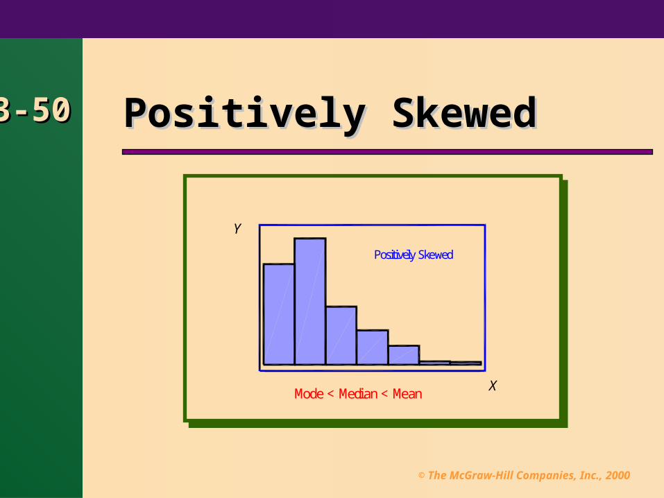
3-503-50 Positively SkewedPositively Skewed

X

Y

Mode < Median < Mean

Positively Skewed


n

3-513-51 SymmetricalSymmetrical

Y

X

Symmetrical

Mean = Media = Mode


Y

X

Negatively Skewed

Mean

3-523-52 Negatively SkewedNegatively Skewed

< Median < Mode


3-533-53 3-3 Measures of Variation - Range3-3 Measures of Variation - Range

The range range is defined to be the highest value minus the lowest value. The symbol RR is used for the range.

RR = highest value – lowest value. = highest value – lowest value. Extremely large or extremely small

data values can drastically affect the range.


3-543-543-3 Measures of Variation - 3-3 Measures of Variation -

Population VariancePopulation Variance

The variance is the average of the squares of the

distance each value is from the mean.

The symbol for the population variance is

( is the Greek lowercase letter sigma)2

=

=

=

2 ( )

,X

Nwhere

X individual value

population mean

N population size

2


3-553-553-3 Measures of Variation - 3-3 Measures of Variation -

Population Standard DeviationPopulation Standard Deviation

The standard deviation is the square

root of the variance.

= 2

( ).

X

N

2


3-563-56

Consider the following data to constitute the population: 10, 60, 50, 30, 40, 20. Find the mean and variance.

The mean mean = (10 + 60 + 50 + 30 + 40 + 20)/6 = 210/6 = 35.

The variance variance 22 = 1750/6 = 291.67. See next slide for computations.

3-3 Measures of Variation -3-3 Measures of Variation - Example


3-573-573-3 Measures of Variation -3-3 Measures of Variation -

Example

X X - (X - )2

10 -25 625

60 +25 625

50 +15 225

30 -5 25

40 +5 25

20 -15 225

210 1750

X X - (X - )2

10 -25 625

60 +25 625

50 +15 225

30 -5 25

40 +5 25

20 -15 225

210 1750


3-583-58

3-3 Measures of Variation - Sample 3-3 Measures of Variation - Sample

Variance Variance

The unbiased estimat or of the population

variance or the sample varianc e is a

statistic whose value approximates the

expected value of a population variance.

It is denoted by s 2 ,

( ),

where

sX X

nand

X sample mean

n sample size

=

=

2

2

1


3-593-593-3 Measures of Variation - Sample 3-3 Measures of Variation - Sample Standard Deviation Standard Deviation

The sample standard deviation is the square

root of the sample variance.

= 2s sX X

n

( ).

2

1


3-603-603-33-3 Shortcut Formula for the Sample for the Sample Variance and the Standard DeviationVariance and the Standard Deviation

=

=

X X nn

sX X n

n

s2

2 2

2 2

1

1

( ) /

( ) /


3-613-61

Find the variance and standard deviation for the following sample: 16, 19, 15, 15, 14.

X = 16 + 19 + 15 + 15 + 14 = 79. X2 = 162 + 192 + 152 + 152 + 142

= 1263.

3-3 Sample Variance -3-3 Sample Variance - Example


=

1263 (79)

= 3.7

= 3.7

2

sX X n

n

s

2

2 2

15

4

19

( ) /

/

. .

3-623-62 3-3 Sample Variance -3-3 Sample Variance - Example


3-633-63

For groupedgrouped data, use the class midpoints for the observed value in the different classes.

For ungroupedungrouped data, use the same formula (see next slide) with the class midpoints, Xm, replaced with the actual observed X value.

3-3 Sample Variance for Grouped 3-3 Sample Variance for Grouped and Ungrouped Dataand Ungrouped Data


3-643-64

The sample variance for grouped data:

=sf X f X n

nm m2

2 2

1

[( ) / ].

3-3 Sample Variance for Grouped 3-3 Sample Variance for Grouped and Ungrouped Dataand Ungrouped Data

For ungrouped data, replace Xm with the observe X value.

For ungrouped data, replace Xm with the observe X value.


3-653-65

X f fX fX2

5 2 10 50

6 3 18 108

7 8 56 392

8 1 8 64

9 6 54 486

10 4 40 400

n = 24 fX = 186 fX2 = 1500

X f fX fX2

5 2 10 50

6 3 18 108

7 8 56 392

8 1 8 64

9 6 54 486

10 4 40 400

n = 24 fX = 186 fX2 = 1500

3-3 Sample Variance for Grouped 3-3 Sample Variance for Grouped DataData -- Example


3-663-66

The sample variance and standard deviation:

=

= 1500 [(186)

2

sf X f X n

n

s

2

2 2

124

232 54

2 54 16

[( ) / ]

/ ]. .

. . .

3-3 Sample Variance for Ungrouped 3-3 Sample Variance for Ungrouped DataData -- Example


3-673-67

The coefficient of variationcoefficient of variation is defined to be the standard deviation divided by the mean. The result is expressed as a percentage.

3-3 Coefficient of Variation3-3 Coefficient of Variation

CVarsX

or CVar 100% 100%. =


3-683-68 Chebyshev’s TheoremChebyshev’s Theorem

The proportion of values from a data set that will fall within k standard deviations of the mean will be at least 1 – 1/k2, where k is any number greater than 1.

For k = 2, 75% of the values will lie within 2 standard deviations of the mean. For k = 3, approximately 89% will lie within 3 standard deviations.


3-693-69 The Empirical (Normal) RuleThe Empirical (Normal) Rule

For any bell shaped distribution: Approximately 68% of the data values will

fall within one standard deviation of the mean.

Approximately 95% will fall within two standard deviations of the mean.

Approximately 99.7% will fall within three standard deviations of the mean.


3-703-70 The Empirical (Normal) RuleThe Empirical (Normal) Rule

-- 95%


3-713-71 3-4 Measures of Position — 3-4 Measures of Position — z z scorescore

The standard scorestandard score or zz score score for a value is obtained by subtracting the mean from the value and dividing the result by the standard deviation.

The symbol zz is used for the zz score score.


3-723-72

The z score represents the number of standard deviations a data value falls above or below the mean.

3-4 Measures of Position — z-score3-4 Measures of Position — z-score

For samples

zX X

sFor populations

zX

:

.

:

.


3-733-73

A student scored 65 on a statistics exam that had a mean of 50 and a standard deviation of 10. Compute the z-score.

z = (65 – 50)/10 = 1.5. That is, the score of 65 is 1.5 standard

deviations aboveabove the mean. Above -Above - since the z-score is positive.

3-4 z-score -3-4 z-score - Example


3-743-743-4 Measures of Position - 3-4 Measures of Position - PercentilesPercentiles

Percentiles divide the distribution into 100 groups.

The PPkk percentile is defined to be that numerical value such that at most k% of the values are smaller than Pk and at most (100 – k)% are larger than Pk in an ordered data set.


3-753-75 3-4 Percentile Formula3-4 Percentile Formula

The percentile corresponding to a given value (X) is computed by using the formula:

Percentilenumber of values below X + 0.5

total number of values

100%


3-763-76 3-4 Percentiles - Example3-4 Percentiles - Example

A teacher gives a 20-point test to 10 students. Find the percentile rank of a score of 12. Scores: 18, 15, 12, 6, 8, 2, 3, 5, 20, 10.

Ordered set: 2, 3, 5, 6, 8, 10, 12, 15, 18, 20. Percentile = [(6 + 0.5)/10](100%) = 65th

percentile. Student did better than 65% of the class.


3-773-773-4 Percentiles - Finding the value 3-4 Percentiles - Finding the value Corresponding to a Given PercentileCorresponding to a Given Percentile

Procedure:Procedure: Let p be the percentile and n the sample size.

Step 1:Step 1: Arrange the data in order. Step 2:Step 2: Compute c c = (= (nnpp)/100)/100. Step 3:Step 3: If cc is not a whole number, round

up to the next whole number. If cc is a whole number, use the value halfway

between cc and cc+1+1.



Step 4:Step 4: The value of c is the position value of the required percentile.

Example: Find the value of the 25th percentile for the following data set: 2, 3, 5, 6, 8, 10, 12, 15, 18, 20.

Note:Note: the data set is already ordered. n = 10, p = 25, so c = (1025)/100 = 2.5.

Hence round up to c = 3.



Thus, the value of the 25th percentile is the value X = 5.

Find the 80th percentile. c = (1080)/100 = 8. Thus the value of the

80th percentile is the average of the 8th and 9th values. Thus, the 80th percentile for the data set is (15 + 18)/2 = 16.5.


3-803-80 3-4 Special Percentiles - Deciles and 3-4 Special Percentiles - Deciles and

QuartilesQuartiles

DecilesDeciles divide the data set into 10 groups.

Deciles are denoted by D1, D2, …, D9 with the corresponding percentiles being P10, P20, …, P90

QuartilesQuartiles divide the data set into 4 groups.


3-813-81 3-4 Special Percentiles - Deciles and 3-4 Special Percentiles - Deciles and

QuartilesQuartiles

Quartiles are denoted by Q1, Q2, and Q3 with the corresponding percentiles being P25, P50, and P75.

The median is the same as P50 or Q2.


3-823-823-4 Outliers and the 3-4 Outliers and the

Interquartile Range (IQR)Interquartile Range (IQR)

An outlieroutlier is an extremely high or an extremely low data value when compared with the rest of the data values.

The Interquartile RangeInterquartile Range, IQR = IQR = QQ33 – – QQ11.


3-833-83 3-4 Outliers and the 3-4 Outliers and the

Interquartile Range (IQR) Interquartile Range (IQR)

To determine whether a data value can be considered as an outlier:

Step 1:Step 1: Compute Q1 and Q3.

Step 2:Step 2: Find the IQR = Q3 – Q1. Step 3:Step 3: Compute (1.5)(IQR). Step 4:Step 4: Compute Q1 – (1.5)(IQR) and

Q3 + (1.5)(IQR).


3-843-843-4 Outliers and the 3-4 Outliers and the

Interquartile Range (IQR)Interquartile Range (IQR)

To determine whether a data value can be considered as an outlier:

Step 5:Step 5: Compare the data value (say X) with Q1 – (1.5)(IQR) and Q3 + (1.5)(IQR).

If X < Q1 – (1.5)(IQR) or if X > Q3 + (1.5)(IQR), then X is considered

an outlier.


3-853-853-4 Outliers and the Interquartile 3-4 Outliers and the Interquartile

Range (IQR) - Range (IQR) - Example

Given the data set 5, 6, 12, 13, 15, 18, 22, 50, can the value of 50 be considered as an outlier?

Q1 = 9, Q3 = 20, IQR = 11. VerifyVerify. (1.5)(IQR) = (1.5)(11) = 16.5. 9 – 16.5 = – 7.5 and 20 + 16.5 = 36.5. The value of 50 is outside the range – 7.5

to 36.5, hence 50 is an outlier.


3-863-863-5 Exploratory Data Analysis - 3-5 Exploratory Data Analysis -

Stem and Leaf PlotStem and Leaf Plot

A stem and leaf plotstem and leaf plot is a data plot that uses part of a data value as the stem and part of the data value as the leaf to form groups or classes.


3-873-87

At an outpatient testing center, a sample of 20 days showed the following number of cardiograms done each day: 25, 31, 20, 32, 13, 14, 43, 02, 57, 23, 36, 32, 33, 32, 44, 32, 52, 44, 51, 45. Construct a stem and leaf plot for the data.

3-5 Exploratory Data Analysis - 3-5 Exploratory Data Analysis - Stem and Leaf Plot - Stem and Leaf Plot - Example


3-883-883-5 Exploratory Data Analysis - 3-5 Exploratory Data Analysis - Stem and Leaf Plot - Stem and Leaf Plot - Example

Leading Digit (Stem) Trailing Digit (Leaf)

0 21 3 42 0 3 53 1 2 2 2 2 3 64 3 4 4 55 1 2 7


3-893-893-5 Exploratory Data Analysis - Box 3-5 Exploratory Data Analysis - Box

PlotPlot

When the data set contains a small number of values, a box plotbox plot is used to graphically represent the data set. These plots involve five values: the minimum valueminimum value, the lower hingelower hinge, the medianmedian, the upper hingeupper hinge, and the maximum valuemaximum value.



PlotPlot

The lower hingelower hinge is the median of all values less than or equal to the median when the data set has an odd number of values, or as the median of all values less than the median when the data set has an even number of values. The symbol for the lower hinge is LHLH.



PlotPlot

The upper hingeupper hinge is the median of all values greater than or equal to the median when the data set has an odd number of values, or as the median of all values greater than the median when the data set has an even number of values. The symbol for the upper hinge is UHUH.


3-923-923-5 Exploratory Data Analysis - Box 3-5 Exploratory Data Analysis - Box Plot - Plot - Example (Cardiograms data) (Cardiograms data)

6050403020100

LH UH

MEDIAN

MINIMUM MAXIMUM


3-933-93 Information Obtained from a Box Information Obtained from a Box Plot Plot

If the median is near the center of the box, the distribution is approximately symmetric.

If the median falls to the left of the center of the box, the distribution is positively skewed.

If the median falls to the right of the center of the box, the distribution is negatively skewed.


3-943-94 Information Obtained from a Box Information Obtained from a Box Plot Plot

If the lines are about the same length, the distribution is approximately symmetric.

If the right line is larger than the left line, the distribution is positively skewed.

If the left line is larger than the right line, the distribution is negatively skewed.

Documents

Bman03 Data Description