Embed Size (px)
Citation preview
Budapest University of Technology and EconomicsFaculty of Electrical Engineering and Informatics
Department of Telecommunications and Telematics
Development and Evaluation of aDynamic Bluetooth Scatternet Formation Procedure
Mark Felegyhazi
Master’s Thesis
Supervisors: Gyorgy Miklos, M.Sc., Ericsson ResearchAndras Racz, M.Sc., Ericsson ResearchEdit Halasz, PhD., Budapest University of Technology and Economics
Budapest, 2001.


Nyilatkozat
Alulırott Felegyhazi Mark, a Budapesti Muszaki es Gazdasagtudomanyi Egyetem hallgatoja
kijelentem, hogy ezt a diplomatervet meg nem engedett segıtseg nelkul, sajat magam keszıtettem,
es a diplomatervben csak a megadott forrasokat hasznaltam fel. Minden olyan reszt, melyet szo
szerint, vagy azonos ertelemben de atfogalmazva mas forrasbol atvettem, egyertelmuen, a forras
megadasaval megjeloltem.
Budapest, 2001. majus ..............................Felegyhazi Mark


Acknowledgment
I want to thank to Gyorgy Miklos and Andras Racz who helped me with advices when “in
the middle of the journey of our life I came to myself within a dark wood where the straight
way was lost” [Dante21]. With their hints I was able to find the way out.
I also want to thank to Edit Halasz, Ph.D. for supervising my work.
Thanks to all the employees of Ericsson Traffic Lab who have helped me to do my work
with pleasure and joy. Thank to the Department of Telematics and Telecommunications, High
Speed Networks Lab and Ericsson Traffic Lab for providing me a good environment for my work.
Especially thanks to all the members of the LIMES project for the advices and for egging me
to get on with my work in the difficult moments.
I would like to thank all of my family for the love and especially for my brother, Csaba for
the additional review of the thesis.
Finally I want send my love to Bogi who stood by me all the time.


Abstract
Personal mobile communication is going to be more and more important. There are many
devices which provide users with connection to each other or to the global communication infras-
tructures like the Internet. The Bluetooth technology provides a short range radio connection
between devices. It can be used instead of different cables.
Bluetooth also enables ad hoc networking with the devices. In this case the devices are able
to form a network without an existing infrastructure. They forward the data for each other
over multiple hops. Such a Bluetooth network is called scatternet. The Bluetooth specification
enables to form scatternets from many devices but it does not specify a protocol for it.
In my thesis I present protocols which can be used for scatternet formation. The Bluetooth
scatternet formation problems can be split up into three parts: connection setup, scatternet
building and scatternet optimization. In my thesis I address the problems of scatternet building
and optimization. I suggest two methods to solve the scatternet building problem. One of the
methods uses limited broadcasting of alive messages. The other method is based on the routing
algorithm. I present an extension with messaging limitation to both methods.
The network building methods keep the network connected but they may not form an efficient
network topology. I developed a scatternet optimization protocol which reconfigures the existing
network topology to reach a more efficient one. Three simple rules are executed based on local
measured traffic information. The aim of every rule is to increase the local capacity of the
network and thereby increase the whole capacity.
To evaluate the protocols I extended the ad hoc Bluetooth simulator in the PLASMA en-
vironment. I present the implementation details of the protocols and a random walk mobility
model. Finally I show simulation results about the scatternet formation protocols. I present how
they form and optimize the scatternet and I point out which parameters affect these procedures.


Kivonat
A szemelyi kommunikacios eszkozok egyre fontosabb szerepet toltenek be a mindennapi
eletben. Ezek az eszkozok osszekottetest biztosıtanak az egyes felhasznalok illetve a felhasznalo
es a globalis halozat kozott is. A Bluetooth technologia egy kis hatosugaru radios technologia,
amely a kulonbozo vezetekes megoldasokkal ellentetben egy egyseges csatlakozasi pontot biztosıt
az eszkozok kozott. A Bluetooth segıtsegevel azonban ad hoc halozatok is felepulhetnek. Az ad
hoc halozatban az eszkozok elore telepıtett infrastruktura segıtsege nelkul alkotnak halozatot.
Ez esetben az eszkozok egyben az utvonalvalaszto szerepet is betoltik. A Bluetooth technologia
eseteben ezt a halozatot scatternetnek nevezik. A Bluetooth szabvany lehetoseget ad a scatternet
felepıtesere, de nem definial ra konkret mechanizmust.
Diplomamunkamban bemutatom az altalam tervezett halozatepıto modszereket. A Blue-
tooth halozatepıtes harom reszre tagolhato: a fizikai kapcsolatfelepıtes, a scatternet epıtes es
a scatternet optimalizalas. Munkam soran a scatternet epıtes es optimalizalas problemajara
fokuszaltam. A halozatepıtes problemajanak megoldasara ket modszert javasolok. Az elso pro-
tokoll eseteben minden eszkoz uzenetekkel jelzi a halozaton az elerhetoseget. A masik modszer
az utvonalvalaszto algoritmusra tamaszkodva donti el, hogy egy adott eszkoz elerheto-e. Amen-
nyiben egy eszkoz radios hatosugaran belul talalhato egy masik, de azt nem eri el, akkor a
ket eszkoz kozvetlen kapcsolatot epıt fel. Mindket modszerhez bemutatok egy kiegeszıtest
korlatozott uzenetkuldessel.
Bar a scatternet epıto modszerek biztosıtjak az osszekotott halozatot, de nem biztos, hogy
az adott halozat elegge hatekony. Ennek megoldasara egy halozat optimalizalo protokollt ter-
veztem, amely egy meglevo topologiat hasznal kiindulopontkent. A protokoll lokalis forga-
lommeres alapjan hajt vegre harom egyszeru szabalyt. A szabalyok vegrehajtasanak celja a
halozat lokalis kapacitasanak novelese ıgy az osszkapacitas novelese.
A tervezett protokollokat szimulacios kornyezetben vizsgaltam. Ehhez kiegeszıtettem a
PLASMA szimulator Bluetooth ad hoc moduljat a halozatepıto protokollokkal es egy veletlen-
szeru mozgasmodellel. Dolgozatom utolso reszeben a protokollok mukodeset mutatom be es azt,
hogy a mukodest milyen valtozokkal lehet befolyasolni.

Contents
1 Introduction 1
1.1 Bluetooth technology . . . . . . . . . . . . . . . . . . . . . . . . . . . . . . . . . . 2
1.2 Ad hoc Bluetooth networks . . . . . . . . . . . . . . . . . . . . . . . . . . . . . . 3
1.3 Structure of the thesis . . . . . . . . . . . . . . . . . . . . . . . . . . . . . . . . . 3
2 Bluetooth wireless technology 4
2.1 Overview of the Bluetooth technology . . . . . . . . . . . . . . . . . . . . . . . . 4
2.2 Ad hoc networking with Bluetooth . . . . . . . . . . . . . . . . . . . . . . . . . . 6
2.3 Open problems regarding Bluetooth networking . . . . . . . . . . . . . . . . . . . 6
2.3.1 Network topology building, maintenance and optimization . . . . . . . . . 7
2.3.2 Routing algorithm optimized for Bluetooth . . . . . . . . . . . . . . . . . 7
2.3.3 Scheduling the communication between nodes . . . . . . . . . . . . . . . . 8
2.4 Proposed architecture for ad hoc networking . . . . . . . . . . . . . . . . . . . . . 9
3 Literature study 11
3.1 Ad hoc network formation using IEEE 802.11 technology . . . . . . . . . . . . . 11
3.2 Published methods for Bluetooth scatternet formation . . . . . . . . . . . . . . . 12
4 Problem formulation 15
4.1 Definition of the scatternet formation problems . . . . . . . . . . . . . . . . . . . 15
4.2 Approach to the scatternet formation problems . . . . . . . . . . . . . . . . . . . 16
4.2.1 Establishing a connection . . . . . . . . . . . . . . . . . . . . . . . . . . . 16
4.2.2 Check reachable neighbours . . . . . . . . . . . . . . . . . . . . . . . . . . 16
4.2.3 Optimization of the scatternet . . . . . . . . . . . . . . . . . . . . . . . . 17
i

5 The network building procedure 19
5.1 Overview of the ABSB method . . . . . . . . . . . . . . . . . . . . . . . . . . . . 19
5.1.1 Periodic broadcast of alive messages . . . . . . . . . . . . . . . . . . . . . 19
5.1.2 Limited alive broadcasting . . . . . . . . . . . . . . . . . . . . . . . . . . . 20
5.2 Detailed description of the ABSB protocol . . . . . . . . . . . . . . . . . . . . . . 21
5.3 Overview of the RBSB method . . . . . . . . . . . . . . . . . . . . . . . . . . . . 24
5.3.1 Routing based scatternet building . . . . . . . . . . . . . . . . . . . . . . 25
5.3.2 Limited routing information based method . . . . . . . . . . . . . . . . . 26
5.4 Detailed description of the RBSB method . . . . . . . . . . . . . . . . . . . . . . 28
6 The network optimization procedure 30
6.1 Overview of the TDSO method . . . . . . . . . . . . . . . . . . . . . . . . . . . . 30
6.2 Two examples of network optimization . . . . . . . . . . . . . . . . . . . . . . . . 31
6.2.1 Example 1: A simple piconet . . . . . . . . . . . . . . . . . . . . . . . . . 31
6.2.2 Example 2: Optimization of a scatternet . . . . . . . . . . . . . . . . . . . 33
6.3 Detailed description of the TDSO protocol . . . . . . . . . . . . . . . . . . . . . . 36
6.3.1 Link setup rule . . . . . . . . . . . . . . . . . . . . . . . . . . . . . . . . . 36
6.3.2 Link master-slave switch rule . . . . . . . . . . . . . . . . . . . . . . . . . 39
6.3.3 Link teardown rule . . . . . . . . . . . . . . . . . . . . . . . . . . . . . . . 40
7 Simulation environment 43
7.1 The Bluetooth ad hoc module . . . . . . . . . . . . . . . . . . . . . . . . . . . . . 43
7.2 Implementation of the random mobility model . . . . . . . . . . . . . . . . . . . 46
7.3 Implementation of the network building method . . . . . . . . . . . . . . . . . . . 46
7.4 Implementation of the network optimization procedure . . . . . . . . . . . . . . . 47
7.5 Scheduling implementation . . . . . . . . . . . . . . . . . . . . . . . . . . . . . . 48
8 Results of the simulation 50
8.1 Investigations of the ABSB protocol . . . . . . . . . . . . . . . . . . . . . . . . . 50
8.1.1 Piconet building with ABSB . . . . . . . . . . . . . . . . . . . . . . . . . 50
8.1.2 Scatternet building with ABSB . . . . . . . . . . . . . . . . . . . . . . . . 53
8.1.3 Increasing the limit of the messaging . . . . . . . . . . . . . . . . . . . . . 53

8.2 Simulation results of the TDSO protocol . . . . . . . . . . . . . . . . . . . . . . . 55
8.2.1 Effect of the Tcheck value . . . . . . . . . . . . . . . . . . . . . . . . . . . . 55
8.2.2 Effect of the Texecution value . . . . . . . . . . . . . . . . . . . . . . . . . . 56
9 Summary 58
Appendices 60
A Dynamic scatternet building with 5 nodes 60

List of Figures
1.1 Cable replacement with Bluetooth . . . . . . . . . . . . . . . . . . . . . . . . . . 2
2.1 Connection establishment in Bluetooth . . . . . . . . . . . . . . . . . . . . . . . . 5
2.2 FHSS/TDD communication between master and slave . . . . . . . . . . . . . . . 5
2.3 Architecture of an example scatternet . . . . . . . . . . . . . . . . . . . . . . . . 6
2.4 Different topologies from the A-B traffic point of view . . . . . . . . . . . . . . . 7
2.5 Example scatternet . . . . . . . . . . . . . . . . . . . . . . . . . . . . . . . . . . . 8
2.6 An example for scheduling mechanism . . . . . . . . . . . . . . . . . . . . . . . . 9
2.7 Architecture of Bluetooth networking protocol . . . . . . . . . . . . . . . . . . . 10
4.1 Open questions regarding scatternet formation . . . . . . . . . . . . . . . . . . . 15
5.1 Steps of the link setup rule . . . . . . . . . . . . . . . . . . . . . . . . . . . . . . 20
5.2 Limited broadcasting in ABSB . . . . . . . . . . . . . . . . . . . . . . . . . . . . 21
5.3 Multiple connected scatternet . . . . . . . . . . . . . . . . . . . . . . . . . . . . . 21
5.4 Example scatternet to present the limited alive broadcasting method . . . . . . . 22
5.5 Alive message . . . . . . . . . . . . . . . . . . . . . . . . . . . . . . . . . . . . . . 22
5.6 Alive message of B reached hop-limit . . . . . . . . . . . . . . . . . . . . . . . . . 23
5.7 Direct connection between B and E . . . . . . . . . . . . . . . . . . . . . . . . . . 24
5.8 Topology stored at every node . . . . . . . . . . . . . . . . . . . . . . . . . . . . 25
5.9 The link failure is spread by the nodes at the end of the broken link . . . . . . . 25
5.10 Node E restores the fully-connected topology . . . . . . . . . . . . . . . . . . . . 26
5.11 Limited link state routing in RBSB . . . . . . . . . . . . . . . . . . . . . . . . . . 27
5.12 The scatternet becomes multiple connected . . . . . . . . . . . . . . . . . . . . . 27
5.13 Limited topology stored at every node . . . . . . . . . . . . . . . . . . . . . . . . 28
iv

5.14 Table update message . . . . . . . . . . . . . . . . . . . . . . . . . . . . . . . . . 28
5.15 Node B and E build up a direct link . . . . . . . . . . . . . . . . . . . . . . . . . 29
6.1 A simple piconet . . . . . . . . . . . . . . . . . . . . . . . . . . . . . . . . . . . . 31
6.2 Connection setup . . . . . . . . . . . . . . . . . . . . . . . . . . . . . . . . . . . . 32
6.3 Master-slave switch . . . . . . . . . . . . . . . . . . . . . . . . . . . . . . . . . . . 32
6.4 Connection teardown . . . . . . . . . . . . . . . . . . . . . . . . . . . . . . . . . . 32
6.5 A more efficient topology . . . . . . . . . . . . . . . . . . . . . . . . . . . . . . . 33
6.6 A scatternet of two piconets . . . . . . . . . . . . . . . . . . . . . . . . . . . . . . 33
6.7 The first modifications in the scatternet . . . . . . . . . . . . . . . . . . . . . . . 34
6.8 Further link modifications . . . . . . . . . . . . . . . . . . . . . . . . . . . . . . . 34
6.9 The last modifications in the scatternet . . . . . . . . . . . . . . . . . . . . . . . 35
6.10 The final topology is formed . . . . . . . . . . . . . . . . . . . . . . . . . . . . . . 35
6.11 A simple piconet . . . . . . . . . . . . . . . . . . . . . . . . . . . . . . . . . . . . 36
6.12 Steps of the link setup rule . . . . . . . . . . . . . . . . . . . . . . . . . . . . . . 37
6.13 Steps of the link master-slave switch rule . . . . . . . . . . . . . . . . . . . . . . . 40
6.14 Steps of the teardown switch rule . . . . . . . . . . . . . . . . . . . . . . . . . . . 41
7.1 Architecture of the PLASMA ad hoc module . . . . . . . . . . . . . . . . . . . . 44
7.2 Timing of the page procedure . . . . . . . . . . . . . . . . . . . . . . . . . . . . . 47
7.3 Random paging mechanism at power up . . . . . . . . . . . . . . . . . . . . . . . 47
8.1 Throughput of a 3-node scatternet . . . . . . . . . . . . . . . . . . . . . . . . . . 51
8.2 Topology reconfigurations in the 3-node scatternet . . . . . . . . . . . . . . . . . 52
8.3 Throughput of a scatternet with 5 nodes . . . . . . . . . . . . . . . . . . . . . . . 53
8.4 The throughput and alive message overhead increasing the scope . . . . . . . . . 54
8.5 A simple piconet topology . . . . . . . . . . . . . . . . . . . . . . . . . . . . . . . 55
8.6 Influence of Tcheck on the throughput . . . . . . . . . . . . . . . . . . . . . . . . . 56
8.7 Influence of Texecution on the throughput . . . . . . . . . . . . . . . . . . . . . . . 57

List of Tables
5.1 Alive message of node B received by node C . . . . . . . . . . . . . . . . . . . . . 23
5.2 Maximum timeout counter reached at node E . . . . . . . . . . . . . . . . . . . . 23
5.3 Topology table of node B . . . . . . . . . . . . . . . . . . . . . . . . . . . . . . . 28
6.1 Forwarded traffic table of node C . . . . . . . . . . . . . . . . . . . . . . . . . . . 36
6.2 Messages of the link setup . . . . . . . . . . . . . . . . . . . . . . . . . . . . . . . 38
6.3 Neighbour traffic table of A . . . . . . . . . . . . . . . . . . . . . . . . . . . . . . 39
6.4 Messages of the master-slave switch . . . . . . . . . . . . . . . . . . . . . . . . . 40
6.5 Neighbour traffic table of A . . . . . . . . . . . . . . . . . . . . . . . . . . . . . . 41
6.6 Messages by link teardown . . . . . . . . . . . . . . . . . . . . . . . . . . . . . . . 41
vi

Chapter 1
Introduction
There is an important trend toward personal mobile communications. People use more and
more handheld devices to keep in touch with friends or business partners. These devices make it
possible to reach the global communication network and the services independent of the physical
location.
A typical device for personal data management is the Personal Digital Assistant (PDA) or
the mobile phone. Often there is a need for connecting the different devices. For example to
synchronize the stored data between our mobile phone and our laptop. There can be other
applications, for example, our mobile phone should be able to call the person whose number we
searched from the phone book of our PDA.
There are different methods to connect portable devices. We can connect devices with cables.
This method has the advantage that the cables enable a relatively high data rate transmission
between the devices but they have the disadvantage that we need different types of cables to
different connections. When one has a mobile phone, a PDA and a laptop then several cables
are needed to connect them.
Another method is to connect the devices via a wireless connection. The first solution was
the infrared technology [IrDA01]. This technology provides connection between different devices
by the using only one infrared interface. However the infrared technology has some drawbacks.
First of all the transmission range is quite small (typically 1-2 m). Furthermore the devices need
to be in line of sight to communicate, which means that there can not be any objects between
the devices. Last but not least the infrared technology can connect only two devices so there is
2 CHAPTER 1. INTRODUCTION
no opportunity for networking.
1.1 Bluetooth technology
We can use wireless radio technology to connect different devices. The emerging Bluetooth
technology [BTspec99, Haartsen98, Miklos00] is a possible solution to connect devices and it
enables networking, too. Firstly it ensures reliable short range radio connection between the
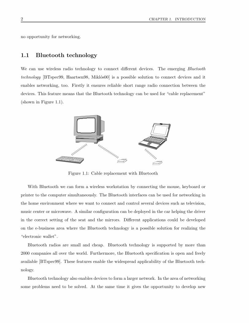
devices. This feature means that the Bluetooth technology can be used for “cable replacement”
(shown in Figure 1.1).
Figure 1.1: Cable replacement with Bluetooth
With Bluetooth we can form a wireless workstation by connecting the mouse, keyboard or
printer to the computer simultaneously. The Bluetooth interfaces can be used for networking in
the home environment where we want to connect and control several devices such as television,
music center or microwave. A similar configuration can be deployed in the car helping the driver
in the correct setting of the seat and the mirrors. Different applications could be developed
on the e-business area where the Bluetooth technology is a possible solution for realizing the
“electronic wallet”.
Bluetooth radios are small and cheap. Bluetooth technology is supported by more than
2000 companies all over the world. Furthermore, the Bluetooth specification is open and freely
available [BTspec99]. These features enable the widespread applicability of the Bluetooth tech-
nology.
Bluetooth technology also enables devices to form a larger network. In the area of networking
some problems need to be solved. At the same time it gives the opportunity to develop new

1.2. AD HOC BLUETOOTH NETWORKS 3
applications. Bluetooth technology enables both connection to a core network (access to the
core network) and direct connection between devices (ad hoc connection).
1.2 Ad hoc Bluetooth networks
Ad hoc networks are networks where the devices do not need any infrastructure to communicate
with each other (as is the case with mobile telephony for example).
The problems concerning ad hoc networks are the issues of the IETF MANET [MANET01]
working group. The working group currently focuses on the standardization of routing algo-
rithms for ad hoc networks. The two candidates for standardization are the Dynamic Source
Routing (DSR) [DSR01] and the ad hoc On-demand Distance Vector (AODV) [AODV01] algo-
rithms.
An important feature of the Bluetooth technology is that it enables ad hoc networking which
means that with Bluetooth capable devices we are able to build up a network without existing
infrastructure. Bluetooth technology provides a possible physical and link layer for ad hoc
networks.
1.3 Structure of the thesis
The structure of my thesis is the following. First, I give an overview of Bluetooth wireless
technology [BTspec99] in Chapter 2. The overview includes the description of the technology
itself and discussion about the open problems regarding ad hoc networking. In the next chap-
ter I present different publications about network formation in ad hoc networks especially in
Bluetooth scatternets (Chapter 3). I split up the scatternet formation problem into two parts:
scatternet building and scatternet optimization. The topics of the next two chapters are my
suggested methods to solve both of these problems (Chapter 5,6). I also performed simula-
tions to evaluate the performance of my methods. I present the simulation environment and
my implementation in Chapter 7. Chapter 8 shows simulation results regarding the developed
methods. In the last chapter I summarize my work (Chapter 9).
Chapter 2
Bluetooth wireless technology
2.1 Overview of the Bluetooth technology
The Bluetooth wireless technology operates in the 2.4-2.5 GHz Industrial, Scientific, Medicine
(ISM) frequency band which is license free. This means that users do not need to pay for the
licence of the usage of the frequency band. But it also means that other radio technologies
and other types of devices (for example the microwave oven) can also use the same frequencies
as Bluetooth. To reduce the interference caused by other devices Bluetooth technology uses
the Frequency Hopping Spread Spectrum (FHSS) [Imre00, WLAN99] method. The transmission
frequency is periodically changed. This feature of the FHSS method gives a robustness against
interference and fading.
Bluetooth standard defines 79 frequencies for communication. The devices use a pseudo-
random sequence to determine the series of the frequency hopping between the channels. The
length of the time slots is 0.625 ms, which means 1600 hops/s hopping speed.
The devices can communicate using a master-slave method. The master role is signed to the
node which determines the frequency hopping scheme in the connection. Up to 7 active slaves
can connect to a master node. This formation is called piconet. Communication in the piconet
is lead by the master which means that the master determines the hopping sequence and the
slaves synchronize their clock to the master’s clock. These roles are only logical states. Any
device can become a master or a slave.
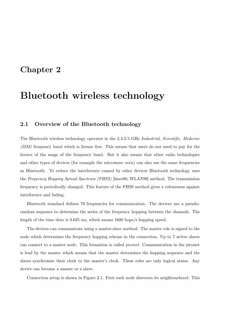
Connection setup is shown in Figure 2.1. First each node discovers its neighbourhood. This
2.1. OVERVIEW OF THE BLUETOOTH TECHNOLOGY 5
process is called inquiry. The execution of the inquiry procedure is not mandatory. It can be
done when a node wants to refresh the information about its neighbourhood. During the inquiry
phase one of the two nodes is in INQUIRY state, the other is in INQUIRY SCAN. The node in
INQUIRY SCAN responds to the INQUIRY of the other node. This way the node in INQUIRY
state notices the presence of the node in INQUIRY SCAN. When the devices want to build up
a connection they begin the page procedure. Similar to the inquiry there are two states: PAGE
and PAGE SCAN. When one of the nodes wants to build up a connection to the other node it
enters in the PAGE state. When the other node is in PAGE SCAN state then the connection
setup is done.
PAGE CONNECTEDINQUIRY
Figure 2.1: Connection establishment in Bluetooth
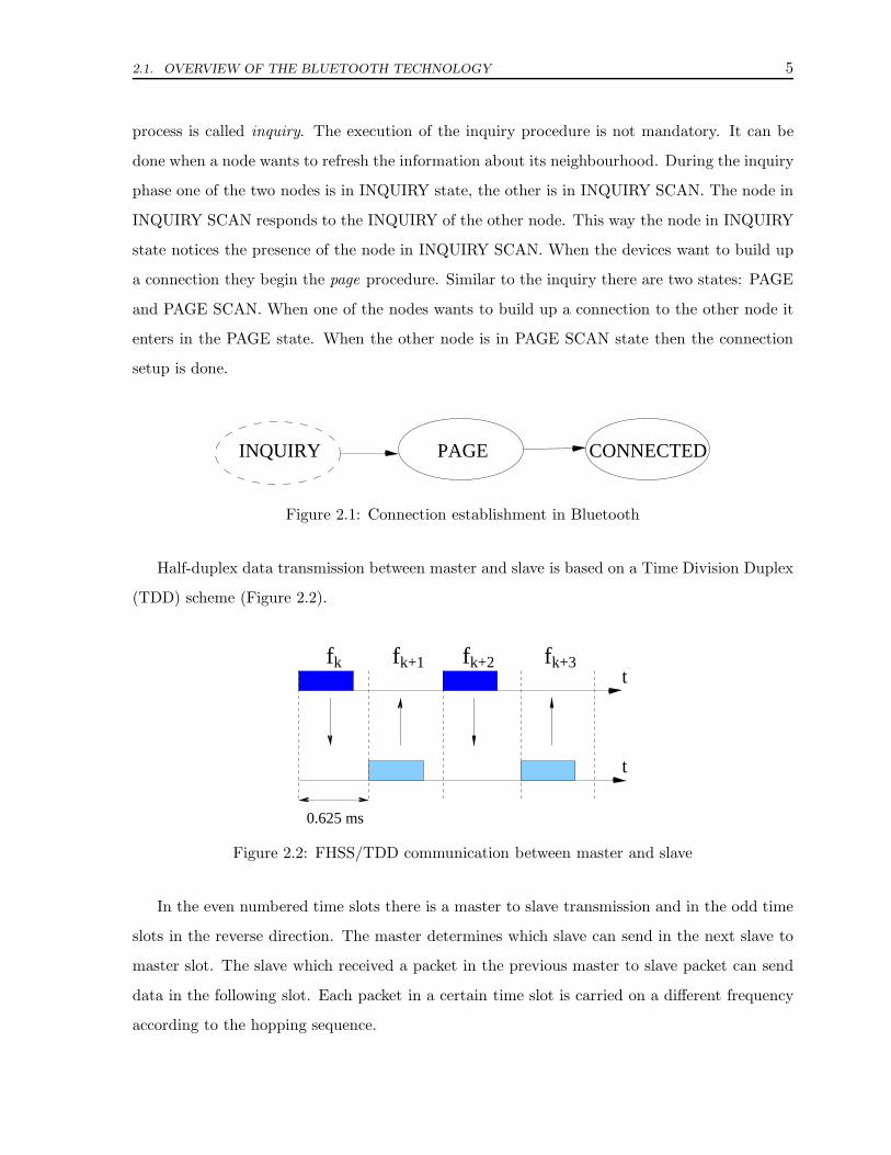
Half-duplex data transmission between master and slave is based on a Time Division Duplex
(TDD) scheme (Figure 2.2).
fk fk+1 fk+2 fk+3t
t
0.625 ms
Figure 2.2: FHSS/TDD communication between master and slave
In the even numbered time slots there is a master to slave transmission and in the odd time
slots in the reverse direction. The master determines which slave can send in the next slave to
master slot. The slave which received a packet in the previous master to slave packet can send
data in the following slot. Each packet in a certain time slot is carried on a different frequency
according to the hopping sequence.
6 CHAPTER 2. BLUETOOTH WIRELESS TECHNOLOGY
2.2 Ad hoc networking with Bluetooth
Besides the point-to-point and point-to-multipoint communication Bluetooth provides the pos-
sibility to build up an ad hoc network of devices.
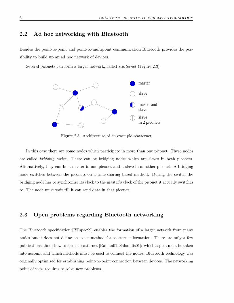
Several piconets can form a larger network, called scatternet (Figure 2.3).
master
slave
slave
slave
master and
in 2 piconets
Figure 2.3: Architecture of an example scatternet
In this case there are some nodes which participate in more than one piconet. These nodes
are called bridging nodes. There can be bridging nodes which are slaves in both piconets.
Alternatively, they can be a master in one piconet and a slave in an other piconet. A bridging
node switches between the piconets on a time-sharing based method. During the switch the
bridging node has to synchronize its clock to the master’s clock of the piconet it actually switches
to. The node must wait till it can send data in that piconet.
2.3 Open problems regarding Bluetooth networking
The Bluetooth specification [BTspec99] enables the formation of a larger network from many
nodes but it does not define an exact method for scatternet formation. There are only a few
publications about how to form a scatternet [Raman01, Salonidis01]: which aspect must be taken
into account and which methods must be used to connect the nodes. Bluetooth technology was
originally optimized for establishing point-to-point connection between devices. The networking
point of view requires to solve new problems.
2.3. OPEN PROBLEMS REGARDING BLUETOOTH NETWORKING 7
2.3.1 Network topology building, maintenance and optimization
The first question is how to build up links between nodes. This means that the piconets must
be determined: the master and slave roles have to be chosen and the bridging nodes have to
be selected. [Racz00] examines the aspects of scatternet formation from an abstract point of
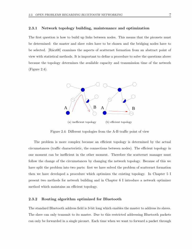
view with statistical methods. It is important to define a procedure to solve the questions above
because the topology determines the available capacity and transmission time of the network
(Figure 2.4).
A B
(a) inefficient topology
A B
(b) efficient topology
Figure 2.4: Different topologies from the A-B traffic point of view
The problem is more complex because an efficient topology is determined by the actual
circumstances (traffic characteristic, the connections between nodes). The efficient topology in
one moment can be inefficient in the other moment. Therefore the scatternet manager must
follow the change of the circumstances by changing the network topology. Because of this we
have split the problem into two parts: first we have solved the problem of scatternet formation
then we have developed a procedure which optimizes the existing topology. In Chapter 5 I
present two methods for network building and in Chapter 6 I introduce a network optimizer
method which maintains an efficient topology.
2.3.2 Routing algorithm optimized for Bluetooth
The standard Bluetooth address field is 3-bit long which enables the master to address its slaves.
The slave can only transmit to its master. Due to this restricted addressing Bluetooth packets
can only be forwarded in a single piconet. Each time when we want to forward a packet through

8 CHAPTER 2. BLUETOOTH WIRELESS TECHNOLOGY
many nodes we have to send the packet to the higher layers which decide where to send the
packet.
Different methods can be used to route the packets. The existing IP routing algorithms
can be applied for the Bluetooth environment, however they were not designed for the ad hoc
environment. The general ad hoc routing methods can also be used like DSDV [DSDV94], DSR
[DSR01] or AODV [AODV01]. The best solution would be to design a Bluetooth specific routing
algorithm but this task is out of scope of my thesis.
2.3.3 Scheduling the communication between nodes
In one single piconet the master decides which slave is allowed to send data in the next slave to
master time slot. To determine which slave can transmit we must use a scheduling algorithm
(intra-piconet scheduling) [NJohan99]. With the scheduling procedure the master of a piconet
determines when the slaves can transmit. This initiation is called polling. During the poll
procedure the master sends poll packets to the slaves.
The problem is more complex when we want to form a scatternet. Figure 2.5 presents an
example scatternet with the scheduling of the slave B during the piconet switch (Figure 2.6).
B
C
A
Figure 2.5: Example scatternet
In this case the master of a piconet has to take the piconet switch of the bridging nodes also
into account (inter-piconet scheduling). The switching time is presented with a gap between the
activity intervals. The node can enter in power save mode (inactive mode). This inactivity is
marked with a longer gap in Figure 2.6. It means that the node must wait till it can send data
in a piconet. The slave assigns an amount of time to spend in a piconet of a master. During
this period the slave waits till the master enables it to send data. The time of the piconet

2.4. PROPOSED ARCHITECTURE FOR AD HOC NETWORKING 9
switch and the waiting time depending on the scheduling determines the whole time which falls
out for communication. This interval means an overhead for the communication. There are
some approaches which realize both functionalities (intra- and inter-piconet scheduling) in one
method [Racz01].
������������
������������
���������������������
���������������������
���������
���������
������
������
���������������������
���������������������
������������������
������������������
���������������
���������������
������
������
������
������
A
B
C
t
t
t
activity intervals for Bin the piconet of A
in the piconet of C
polling ofmaster A
polling ofmaster Cwith Candwith Acommunication intervals for B
Figure 2.6: An example for scheduling mechanism
2.4 Proposed architecture for ad hoc networking
A proposed networking protocol architecture using the Bluetooth as link layer technology is
shown in Figure 2.7.
The user plane shows that the general networking protocols (User Datagram Protocol, UDP
and Transmission Control Protocol, TCP [Tannen96, Stevens94]) operate over Bluetooth. Figure
2.7b shows my suggestion for the control plane.
I suggest the Bluetooth management to be realized by the scatternet manager layer in the
control plane. The main task of the scatternet manager is to build up a network and modify it
if necessary. The scatternet manager solves the problem how to connect a device to the network
and how to release the connection. Since we handle mobile wireless links, the scatternet manager
has to update the topology during the movements of the nodes. The scatternet manager may

10 CHAPTER 2. BLUETOOTH WIRELESS TECHNOLOGY
TCP UDP
BLUETOOTH
LINK LAYER
BLUETOOTHPHYSICAL LAYER
NETWORK LAYER
(a) user plane
BLUETOOTH
PHYSICAL LAYER
SCATTERNET MANAGER
BLUETOOTH
LINK LAYER
NETWORK LAYER
(b) control plane
Figure 2.7: Architecture of Bluetooth networking protocol
realize a routing algorithm specific for Bluetooth network which can be more efficient than a
general ad hoc routing mechanism. It must also control the communication between the nodes
(scheduling). In the following chapters I am going to present these problems in details.
In my thesis I focus on the first problem, that is, how to build up a scatternet and how to
maintain the connection in an existing network. I do not address efficient routing specific for
Bluetooth or scheduling algorithms.

Chapter 3
Literature study
The importance of the problem of Bluetooth scatternet formation has increased in the recent
months. Because this is a new problem there are only few publications about ad hoc network
formation and especially about Bluetooth scatternet formation. In the next section I present a
published method for ad hoc network formation using IEEE 802.11 which is broadcast media
oriented. I give arguments why this method is unable to solve the Bluetooth scatternet formation
problem. In Section 3.2 I focus on some methods which solve the scatternet formation problem.
The problem of network formation includes several parts. First question is how to build up
a connection according to the link layer technology used. When a network is built up we have
to provide the possibility of communication in the network. This means we must handle new
members and link disconnections.
3.1 Ad hoc network formation using IEEE 802.11 technology
The ad hoc network formation problem is strongly dependent on which radio technology is used.
In the case of the IEEE 802.11 standard [Imre00] the communication uses the broadcast radio
medium which means that the devices use the same radio frequency for the communication. In
one moment only one device can use the radio frequency. The devices use the Carrier Sense
Multiple Access with Collision Avoidance (CSMA/CA) protocol [Imre00] to allocate time on the
transmission channel.
The communication is connectionless which results that there is no need for connection
setup. In spite of the lack of connectivity information every node may need to know which other

12 CHAPTER 3. LITERATURE STUDY
nodes are reachable through the network. This problem can be solved with a group membership
mechanism.
The authors of [Roman01] suppose that there is a broadcast medium for the communica-
tion. [Roman01] presents an approach for maintaining group membership information in ad hoc
networks using broadcast media for communication (for example 802.11). The method uses the
coordination information to determine a logical connectivity graph. This graph is a subgraph
of the physical connectivity graph. In every connected network part there is a leader which is
elected through a three-phase leader election mechanism. The leader determines the members
of a group (the members of the logical connectivity graph). The leader knows the speed and
location of every node in the group. The algorithm uses the value of a secure transmission area.
Whenever a node is out of this area it is assigned by the leader as detached from the group.
This way the leader logically disconnects the member from the group before the physical link
teardown. The approach gives a solution for merger and partitioning of the groups. Furthermore
there is a solution for leader election, too.
However this solution made such assumptions which were hard to realize. First of all the
solution uses the location information to determine the secure transmission range for the nodes.
This assumes that the device is able to determine its location. The Global Positioning System
(GPS) [Parkinson95] can be used but this needs a very exact positioning of the device. A local
positioning system can also be used in the indoor environment. Otherwise the procedure has
another disadvantage because of its coordinated nature. When a leader of a group disappears
then the procedure does not work well.
3.2 Published methods for Bluetooth scatternet formation
The Bluetooth technology defines a connection-oriented communication between the nodes which
means that the link must be set up before the communication can begin (paging). This means
that the nodes must begin the configuration of the network only based on the visibility infor-
mation (inquiry) without communicating with each other before.
The differences between Bluetooth networks and other networks are emphasized in [Raman01]
as follows:

3.2. PUBLISHED METHODS FOR BLUETOOTH SCATTERNET FORMATION 13
• Spontaneous network: This means the Bluetooth networks are ad hoc networks. The nodes
do not need an infrastructure to form a network. They forward the packets of each other.
The nodes must also maintain the membership information.
• Isolation: The Bluetooth nodes can not rely on infrastructure based services such as
Domain Name Service (DNS) [Tannen96]. They must operate with distributed methods.
• Simple devices: The devices are planned to be cheap. They have low computational and
battery resources. This means that every approach must take the power save as a strong
requirement into account.
• Small multi-hop networks: The Bluetooth networks should be small networks. There
should not be more members than about some hundred nodes. The packet forwarding is
done by the nodes themselves.
• Connection-oriented technology: Each link which is used for communication must be built
up before. This means that a cost of the active link is relatively high from the power
resources point of view. A solution should make an effort on reducing the number of
active links needed.
[Raman01] suggests an application-based method. The algorithm is an on-demand approach
which means that it builds up links only when they are needed for a specific application. The
authors do not require the connectivity of the network each and every moment. They define a
service caching method instead. During the operation every node stores the information when
its links are needed and makes them active only at these timepoints. The nodes execute a
proposed service discovery procedure to get information about the services of other nodes.
This proposal focuses on the scatternet formation from the services point of view. It has the
advantage that it suggests a method which saves the energy resources of the nodes. However
this approach needs to define the services in each of the nodes before the communication. It is
efficient only in the case of services which need a periodic messaging in predictable timepoints.
The method could be inefficient in the case of unpredictable on-demand communication between
different nodes.

14 CHAPTER 3. LITERATURE STUDY
Another method is published in [Salonidis01] which is a solution focusing on scatternet
formation. The authors propose a protocol which realizes a coordinated approach. In the
coordinator election phase the nodes make a competition to determine the coordinator in the
scatternet. After the coordinator is chosen it determines the configuration of the scatternet. It
forms a temporary piconet for the masters of the later scatternet. It sends the list of the slaves
of that master to each of the nodes. Next the coordinator terminates this temporary piconet
and the master nodes page its slaves. This way the scatternet is formed.
This method addresses the problem of scatternet formation however it has some disadvan-
tages. Firstly it is a centralized approach and shares the drawbacks described in the previous
section. The method needs to be repeated whenever a new node enters or a link tears down.
There is no efficient method how to recalculate the network topology. It means that the proposal
does not address the problem of scatternet maintenance, only the scatternet building. Another
shortcoming of the protocol is that it assumes a network conference scenario where every node
is in the radio range of all others. This limits the usage of the method in general cases.
Chapter 4
Problem formulation
4.1 Definition of the scatternet formation problems
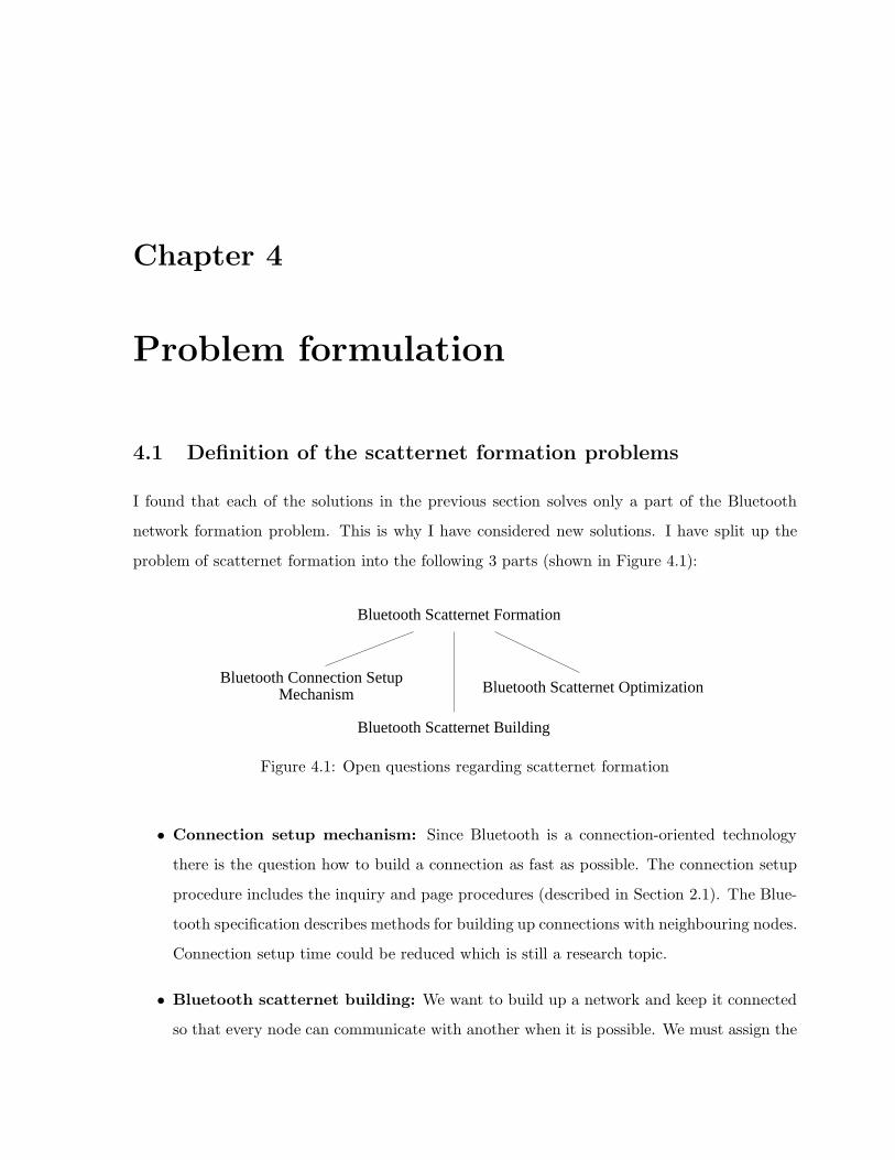
I found that each of the solutions in the previous section solves only a part of the Bluetooth
network formation problem. This is why I have considered new solutions. I have split up the
problem of scatternet formation into the following 3 parts (shown in Figure 4.1):
Bluetooth Scatternet Formation
Bluetooth Scatternet Optimization
Bluetooth Scatternet Building
Bluetooth Connection SetupMechanism
Figure 4.1: Open questions regarding scatternet formation
• Connection setup mechanism: Since Bluetooth is a connection-oriented technology
there is the question how to build a connection as fast as possible. The connection setup
procedure includes the inquiry and page procedures (described in Section 2.1). The Blue-
tooth specification describes methods for building up connections with neighbouring nodes.
Connection setup time could be reduced which is still a research topic.
• Bluetooth scatternet building: We want to build up a network and keep it connected
so that every node can communicate with another when it is possible. We must assign the

16 CHAPTER 4. PROBLEM FORMULATION
master and slave roles and we must determine which nodes bridge between piconets.
Due to the movement of the nodes the existing links can be broken. In this case we must
maintain the network topology to prevent the network from being split into two parts. So
we must replace the broken link with an alternative path. To ensure the reachability of
each node in the network it is sufficient to provide the reachability of every visible node.
This means when a node can reach its visible neighbours then it can reach the visible
neighbours of these nodes, too, and so on.
• Bluetooth scatternet optimization: The network building procedure ensures a fully-
connected scatternet. However this topology can be inefficient in some cases (see Figure
2.4). The scatternet builder modifies the topology only when a link failure occurs. To reach
a more efficient topology I have given an additional feature to the scatternet formation: this
is the scatternet optimization. The scatternet optimization procedure makes the existing
topology more efficient. The traffic carried by the network is forwarded on a shorter path
which increases the capacity of the whole network.
4.2 Approach to the scatternet formation problems
4.2.1 Establishing a connection
The node can explore which other nodes are in visibility range. This procedure is called inquiry
(see Section 2.1). When the node knows its visible neighbours then it is able to choose which
nodes to connect with. This decision is made by the scatternet building procedure which is
described in Chapter 5. In my thesis I use these general methods to build up a connection. I do
not focus on how to improve the connection establishment procedure.
4.2.2 Check reachable neighbours
When the node has built up connection to its neighbour nodes in radio range then it has to
maintain the information whether these nodes are reachable through the network links or not.
If the node can reach its visible neighbours and its neighbours can reach other nodes then the
node can reach other nodes out of its radio range through its neighbours. This way the node is
able to reach all nodes in the network.

4.2. APPROACH TO THE SCATTERNET FORMATION PROBLEMS 17
The power up case is a special case for the scatternet builder methods. It means the node
can not reach any visible neighbours at all. In this case the node schedules a page for all the
visible nodes for a random time. After that time is elapsed the node checks the reachability of
the visible neighbour once more. When the node has become reachable then the node stops the
paging. Otherwise it pages the visible neighbour.
I have developed two methods for scatternet building. In case of Alive Broadcasting Scat-
ternet Builder (ABSB) method the node uses alive messages to inform other nodes about its
presence. The node broadcasts these messages with a scope which is defined in the protocol im-
plementation. The other method is called Routing Based Scatternet Builder (RBSB). Here the
nodes maintain the reachability information based on the information of the routing algorithm.
My solution uses a link state routing algorithm to store the topology in a pre-defined radius.
These methods are described in Chapter 5.
4.2.3 Optimization of the scatternet
To make the scatternet more efficient I suggest a scatternet optimization method called Traffic
Dependent Scatternet Optimizer (TDSO). The TDSO method is based on the idea that the topol-
ogy optimization should take place in a distributed way. Each of the nodes initiates topology
modification according to local measured traffic information. The TDSO procedure is presented
in Chapter 6.
In contrast to the methods [Roman01, Salonidis01] I have developed distributed solutions
for both methods where there is no global coordination between the nodes. A local decision
is made by some nodes together. Each node executes the maintenance and optimization pro-
cedures based on local information without knowing the whole network topology. This feature
makes the solutions robust against the sudden disappearance of a node. The reconfiguration
messages are sent periodically which results in methods that are robust against packet loss.
Whenever a control packet is lost then the maintenance or optimization step will be repeated in
a certain period. In contrast to the idea in [Raman01] my solution provides a connected network
continually. This way there is no need for service discovery and programming of services in each
node.

18 CHAPTER 4. PROBLEM FORMULATION
In my thesis I will use various terms to describe the neighbourhood of a node. I use visible
nodes or visibility neighbours for the nodes which are in radio range. The nodes which are
not connected with a direct link but are still reachable through the existing network are called
reachable nodes. The nodes that have a direct link with the node are the neighbour nodes or
simple neighbours.

Chapter 5
The network building procedure
In this chapter I present a procedure that builds up the Bluetooth network. This is achieved by
the reachability check algorithms. I suggest two methods which are able to coordinate the link
setups between the nodes. In the first section I give an overview (see Section 5.1) of the Alive
Broadcasting Scatternet Builder (ABSB) method with examples. Section 5.2 provides a detailed
description of the method. In Section 5.3 I present an overview of the Routing Based Scatternet
Builder (RBSB) protocol. This is followed by the detailed description of the method in Section
5.4.
5.1 Overview of the ABSB method
In the following I describe the alive broadcasting scatternet builder method (Section 5.1.1). I
also present its variants with signaling limitation in Section 5.1.2.
5.1.1 Periodic broadcast of alive messages
We can check the reachability of the visible nodes by sending periodically refresh messages which
we call alive messages. When the node has periodically refreshed information about all the nodes
in its neighbourhood then it can react to link failures.
The basic rule is that when a node does not receive alive messages from a visible neighbour
then it builds up a link with it (that is, it pages the visible node).
Figure 5.1a shows an example scatternet where the nodes B and E are visible neighbours to
each other. They do not build up a link because they can reach each other through the nodes

20 CHAPTER 5. THE NETWORK BUILDING PROCEDURE
C and D.
A
C
B
D
E
G
F
(a) Example scatternet to il-lustrate the network building
G
F
D
E
A
C
B
(b) Representing the alivemessages of B and E
A
C
B
D
E
G
F
(c) The link between C and Dbreaks down
A
C
B
D
E
G
F
(d) Restoration of the connec-tivity of the scatternet
Figure 5.1: Steps of the link setup rule
In Figure 5.1b the alive messages of the nodes B and E are emphasized. Assume now that
C-D link breaks (Figure 5.1)c. This causes that the nodes B and E do not receive the alive
messages from each other anymore. After a certain time (which depends on the implementation
of the timeout interval) one of the nodes notices that the other node is visible but not reachable
and initiates a connection establishment with the other node. In our case E builds up a link to
B as shown in Figure 5.1d and the network is fully-connected again.
5.1.2 Limited alive broadcasting
We can limit the broadcasting of alive messages (the limit called scope).With the scope value
we can tune the hop distance of the reachability advertisements of the node.

5.2. DETAILED DESCRIPTION OF THE ABSB PROTOCOL 21
In the scatternet in Figure 5.2 the scope is limited to 2. I show only the alive messages of
the nodes B and F in the figure. The nodes are in the visibility range of each other.
C D
A F
E
G
B
Figure 5.2: Limited broadcasting in ABSB
Still, they build up a direct link to each other (Figure 5.3) because the alive messages of B
can not reach F and vice versa.
C D
A F
E
G
B
Figure 5.3: Multiple connected scatternet
The scope of the messaging can be set arbitrarily. The algorithm builds up a new link even
to nodes which are already reachable, but not in the limited scope. Thus a low scope value leads
to a certain redundancy in the network. I examine this effect in Section 8.1.3.
5.2 Detailed description of the ABSB protocol
In this section I describe the alive broadcasting algorithm presented in Section 5.1 including
messages and tables. I focus on the method how to build up a network when the nodes know
which other nodes are in visibility range. I suppose that the nodes get the address and clock

22 CHAPTER 5. THE NETWORK BUILDING PROCEDURE
offset information of every visible node during the inquiry phase. Based on this information the
node is able to build up a new connection to any visible neighbour (paging).
I present the limited version of the method. It is obvious that the broadcasting of messages
in the whole network is a special case of the limited method (limitation is infinity).
I use the example scatternet in Figure 5.1a once more to give a detailed description of the
ABSB protocol (Figure 5.4).
A
C
B
D
E
G
F
Figure 5.4: Example scatternet to present the limited alive broadcasting method
Every node sends alive messages to its neighbours (Figure 5.5). In this case the messaging
limitation is 2 which is determined by the HL (hop-limit) value. The HL value is written in
the TTL field of the alive message. This TTL field is decreased at every node till 0 is reached.
When TTL becomes 0 the node does not forward the message anymore.
SourceBT Address
Time to Live
Figure 5.5: Alive message
The interval between two sending is fixed in the Ts (sending period) parameter. Whenever a
node does not receive alive message from a visible node for a Tto timeout period then it tries to
build up a direct link to that visible neighbour. This fact is checked every Tc (checking period)
seconds. The node pages every visible neighbour that is out of the scope (as shown in Figures
5.2 and 5.3). The implementation of the procedure is presented in Section 7.3.
Let us consider the alive messages of B. C receives the message and processes the reception

5.2. DETAILED DESCRIPTION OF THE ABSB PROTOCOL 23
by setting the Crec bit to one in the reachability table (shown in Table 5.1).
Visible neighbours Crec Cto
A 0 0B 1 0D 0 0
Table 5.1: Alive message of node B received by node C
Next, C checks if the hop-limit of the message is reached (in our case not yet) and decreases
the TTL value by one and forwards the message on every link except the one from which the
message was received.
When D receives the alive message of B it executes the same mechanism as C above, but
without sending the message further (see Figure 5.6).
FA
C
B
D
E
G
Figure 5.6: Alive message of B reached hop-limit
Due to the scope value E does not receive the alive message of B. It increases the Cto counter
at every reachability table check. After the Tto value is reached as shown in Table 5.2 node E
builds up a connection to B (Figure 5.7). In this case the maximum value for Cto is 4.
Visible neighbours Crec Cto
B 0 4D 1 0G 1 0F 0 0
Table 5.2: Maximum timeout counter reached at node E
Figure 5.7 shows that the nodes B and E have built up a redundant link in the network

24 CHAPTER 5. THE NETWORK BUILDING PROCEDURE
G
E
F
B
C D
A
Figure 5.7: Direct connection between B and E
because they can not reach each other. This was caused by the low scope value. Additional links
provide shorter communication routes in the network which enables faster traffic forwarding.
5.3 Overview of the RBSB method
In this section I explain the routing based method for scatternet building. I introduce a link
state method (RBSB) and its variant with message sending limitation.
We can use a proactive distance vector (for example DSDV [DSDV94]) or link state (for
example OLSR [OLSR00]) routing algorithm to explore the topology. With the help of this
knowledge we can react fast to topology changes because the nodes are able to decide whether
a new link is needed or not.
The link state routing algorithm maintains the whole network topology and can calculate the
route to every destination. Every node periodically sends hello messages on its links with the
list of its neighbours. The neighbour nodes store this information and send the message further.
This way every node explores the whole network topology. The Dijkstra-algorithm [Dijkstra59]
can be used to find the shortest path and route the data packets to a destination. The link
failure is detected by one of the end nodes and the information is spread in the network with the
broadcasting of topology refresh messages. When a node refreshes the topology information and
does not find an alternative route instead of the previous route, it builds up a new connection
to one of the unreachable nodes.
5.3. OVERVIEW OF THE RBSB METHOD 25
5.3.1 Routing based scatternet building
I suggest RBSB as a routing based solution. This algorithm uses a link state routing algorithm
to maintain the reachability information.
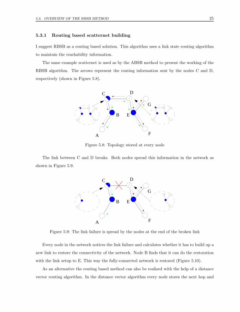
The same example scatternet is used as by the ABSB method to present the working of the
RBSB algorithm. The arrows represent the routing information sent by the nodes C and D,
respectively (shown in Figure 5.8).
B
F
E
G
C D
A
Figure 5.8: Topology stored at every node
The link between C and D breaks. Both nodes spread this information in the network as
shown in Figure 5.9.
EB
F
G
A
C D
Figure 5.9: The link failure is spread by the nodes at the end of the broken link
Every node in the network notices the link failure and calculates whether it has to build up a
new link to restore the connectivity of the network. Node B finds that it can do the restoration
with the link setup to E. This way the fully-connected network is restored (Figure 5.10).
As an alternative the routing based method can also be realized with the help of a distance
vector routing algorithm. In the distance vector algorithm every node stores the next hop and

26 CHAPTER 5. THE NETWORK BUILDING PROCEDURE
B
E
F
G
DC
A
Figure 5.10: Node E restores the fully-connected topology
the distance to each node in the network. When a link failure occurs then a route error is sent to
all of the nodes which are using the link to reach another nodes. This method has the advantage
that the algorithm does not send messages to all of the nodes only to the subset of nodes which
has used the broken link. When these nodes receive the route error message then begin to search
an alternative route to the lost destination. An existing distance vector routing algorithm can
be used, for example Ad-Hoc On-Demand Distance Vector Routing (AODV) [AODV01].
5.3.2 Limited routing information based method
We can make a restriction for the routing based algorithm to reduce the control message over-
head. In this suggestion the node does not explore the whole topology, only its neighbourhood
with a certain exploring radius (here the exploring radius means a hop number). This means
the topology knowledge by the exploring radius in the case of the link state algorithm and the
storage of the nodes which are in the exploring radius in the case of the distance vector algo-
rithm. Figure 5.11 shows a scatternet with limited link state routing information. The exploring
radius is 2.
The limited spreading of topology information implies a direct link setup between B and F
(Figure 5.12).
The exploring radius is tunable and this way we can make a tradeoff between the control
message overhead and the redundancy of the network. When a node does not reach another
visible node through a route whose length is within the exploring radius it builds up a connection
to that particular node. In the example other connections can be also built up. For example
when B and E or C and E are in radio range of each other.

5.3. OVERVIEW OF THE RBSB METHOD 27
C D
A F
E
G
B
Figure 5.11: Limited link state routing in RBSB
C D
A F
E
G
B
Figure 5.12: The scatternet becomes multiple connected
This method is similar to the principle of the Intra-zone Routing Protocol (IARP) [Haas01]
idea which is an extension of the Zone Routing Protocol (ZRP) [Pearlman99]. [Pearlman99]
describes a protocol which is proactive in a certain exploring radius (called zone). As a possible
solution for this protocol [Haas01] is suggested. Outside the zone the ZRP protocol is extended
with an on demand part which realizes reactive search for the destination. The IARP has the
same mechanism as the RBSB protocol with limitation.
Another limited discovery solution is the Fisheye State Routing algorithm (FSR) [Pei00]
where we can set different radius values. In case of the FSR method every node spreads the
neighbour information as usual. The difference between a general link state algorithm and FSR
is that FSR send the the topology information less frequently for the nodes which are more hops
away. For example the node sends the list of every neighbours with the limitation of one in
every second (it means to the neighbours). In every third second it sets the limitation to three.
This way the node sends the topology information to the more distant nodes, too, however with
a lower frequency.

28 CHAPTER 5. THE NETWORK BUILDING PROCEDURE
5.4 Detailed description of the RBSB method
Let us consider the example scatternet from Figure 5.8 with a limited messaging. Every node
has a limited knowledge of the topology with the exploring radius 2 (Figure 5.13). The nodes
periodically send the topology information in table update messages (Figure 5.14) with the period
Ts. The table update messages of the nodes B and E are shown in Figure 5.13. The table update
message contain the address of all neighbouring nodes.
EB
F
G
DC
A
Figure 5.13: Limited topology stored at every node
SourceBT Address Neighbour 1 ... Neighbour N Time to Live
Figure 5.14: Table update message
When a node (for example B) receives a topology update message from a neighbour node (C)
then it updates its topology table (shown in Table 5.3) according to the neighbour information
received from the source node. Afterwards it forwards the message to its neighbours except for
the node from which it has received the message.
Node Neighbour 1 Neighbour 2 ... Neighbour NA B - ... -C B D ... -D C E ... -
Table 5.3: Topology table of node B
Due to the limited topology knowledge the nodes B and E do not reach each other. If they
are visible neighbours, they build up a direct connection as shown in Figure 5.15.

5.4. DETAILED DESCRIPTION OF THE RBSB METHOD 29
B
E
F
G
DC
A
Figure 5.15: Node B and E build up a direct link
The same network configuration is reached as in the example of the ABSB protocol. This
network contains redundant links.

Chapter 6
The network optimization procedure
In this chapter I describe the Traffic Dependent Scatternet Optimizer (TDSO) procedure. First
I present an overview of the network optimization procedure in Section 6.1. In the next section
I present two examples for the optimization procedure: an optimization of the piconet and an
optimization of a scatternet (Section 6.2). This is followed by the detailed description of the
TDSO protocol in Section 6.3.
6.1 Overview of the TDSO method
The network topology optimization algorithm is a distributed method. In the case of the dis-
tributed method there is no need for global coordination. It means that the nodes periodically
execute the rules independently from each other. This operation of the nodes is based on local
traffic information measured at the node. The aim with the execution of the rules is to increase
the network capacity in a local environment and so increase the whole capacity of the network .
I developed a method which optimizes the existing network topology with the execution of
3 basic rules. These rules are executed by every node periodically.
• The first rule builds up new links to reduce the path length of the communication.
• The second rule tears down an unnecessary link when the nodes on both end agree.
• The third rule allows a slave to initiate a master-slave switch. When it is accepted by the
master then the roles are changed.

6.2. TWO EXAMPLES OF NETWORK OPTIMIZATION 31
Every node attempts to change topology according to one of the above rules. In case of
failure, the node re-tries it after a certain period of time. Whenever a link modification step
is accepted the node executes the next step. When a step is not accepted then the node does
not do anything. This means that the steps do not need any acknowledgment, which makes the
procedure robust against packet loss.
6.2 Two examples of network optimization
This section presents two example network optimization series. The aim of showing the examples
is to show how the nodes can cooperate with the execution of the optimization rules. The first
example is a simple piconet of three nodes where the master node forwards traffic between its
two slaves. The second network is more complex involving two piconets. In both cases I suppose
that all of the nodes are within radio range to each other so there is the possibility to build up
a direct link between the nodes which communicate.
6.2.1 Example 1: A simple piconet
A : 100 kb/sC B
B
C
A
Traffic :
Figure 6.1: A simple piconet
In the example piconet shown in Figure 6.1 there is a master node which forwards traffic
between its slaves. When the slaves are in visibility range to each other it would be more efficient
to connect these slaves with a direct link. The master measures the traffic between the nodes
A and B and decides to initiate a link setup between them. When both nodes accept the link
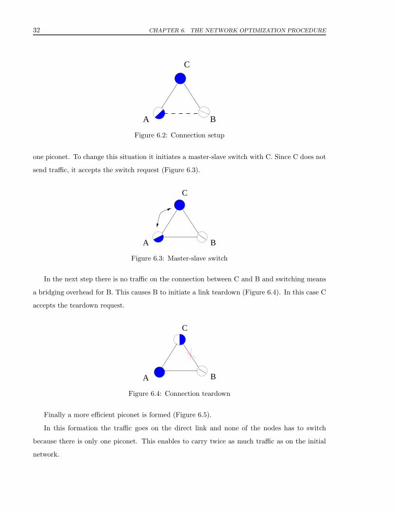
setup (and they are visible to each other) the direct link will be set up (Figure 6.2).
I suppose that the packets are redirected from the route through C to the new link. After
the link setup node A must switch between two piconets even though it forwards traffic only in
32 CHAPTER 6. THE NETWORK OPTIMIZATION PROCEDURE
C
A B
Figure 6.2: Connection setup
one piconet. To change this situation it initiates a master-slave switch with C. Since C does not
send traffic, it accepts the switch request (Figure 6.3).
A
C
B
Figure 6.3: Master-slave switch
In the next step there is no traffic on the connection between C and B and switching means
a bridging overhead for B. This causes B to initiate a link teardown (Figure 6.4). In this case C
accepts the teardown request.
A
C
B
Figure 6.4: Connection teardown
Finally a more efficient piconet is formed (Figure 6.5).
In this formation the traffic goes on the direct link and none of the nodes has to switch
because there is only one piconet. This enables to carry twice as much traffic as on the initial
network.

6.2. TWO EXAMPLES OF NETWORK OPTIMIZATION 33
A B
C
Figure 6.5: A more efficient topology
We saw that the network optimization is done by executing simple rules. The rules reformed
the piconet to reach a more efficient traffic forwarding. Every topology reconfiguration rule
modifies the network topology locally in a distributed manner.
6.2.2 Example 2: Optimization of a scatternet
In the following I present the optimization procedure of a scatternet shown in Figure 6.6.
A
B
CD
E
F
G
Figure 6.6: A scatternet of two piconets
In this network there are two node pairs which communicate. Node A communicates with
node F and node B with G. Both traffic flows are forwarded by node D. Node D presents a
bottleneck for the communication because both traffic flows go through this node. Furthermore
the node has a capacity reduction because of the switching between the two piconets.
Node C notices that it forwards two traffic flows and it initiates a link setup between A and
D. When it is accepted by both nodes they build up a direct link to each other. The same link
setup procedure occurs between C and E initiated by D (Figure 6.7.a). The routing algorithm
relays the traffic to the new links.
The links between A and C and between C and D can be torn down (Figure 6.7.b) because
34 CHAPTER 6. THE NETWORK OPTIMIZATION PROCEDURE
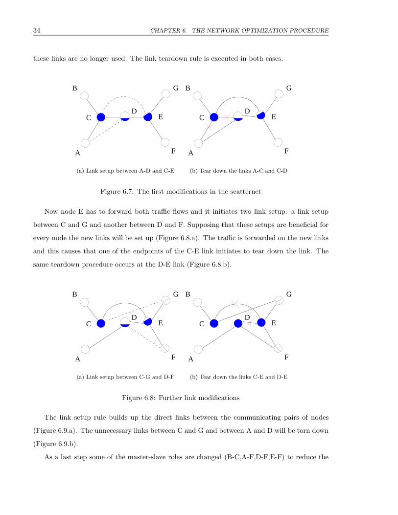
these links are no longer used. The link teardown rule is executed in both cases.
A
B
CD
E
F
G
(a) Link setup between A-D and C-E
A
B
CD
E
F
G
(b) Tear down the links A-C and C-D
Figure 6.7: The first modifications in the scatternet
Now node E has to forward both traffic flows and it initiates two link setup: a link setup
between C and G and another between D and F. Supposing that these setups are beneficial for
every node the new links will be set up (Figure 6.8.a). The traffic is forwarded on the new links
and this causes that one of the endpoints of the C-E link initiates to tear down the link. The
same teardown procedure occurs at the D-E link (Figure 6.8.b).
A
B
CD
E
F
G
(a) Link setup between C-G and D-F
A
B
CD
E
F
G
(b) Tear down the links C-E and D-E
Figure 6.8: Further link modifications
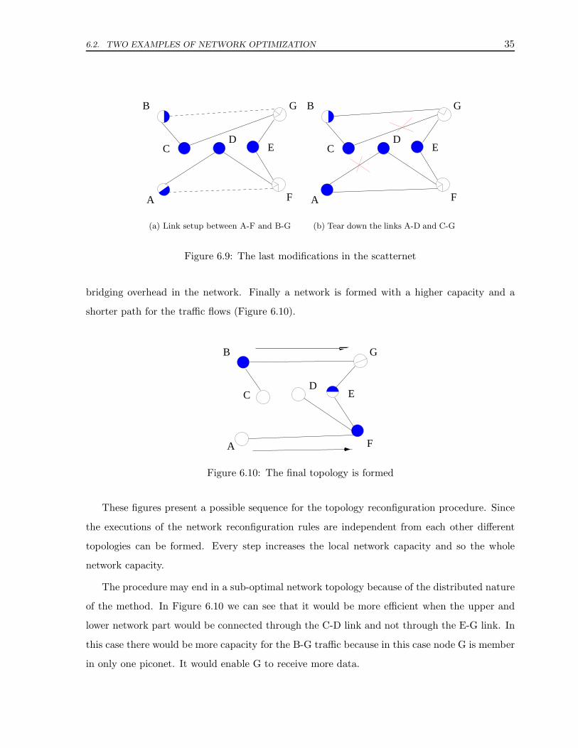
The link setup rule builds up the direct links between the communicating pairs of nodes
(Figure 6.9.a). The unnecessary links between C and G and between A and D will be torn down
(Figure 6.9.b).
As a last step some of the master-slave roles are changed (B-C,A-F,D-F,E-F) to reduce the
6.2. TWO EXAMPLES OF NETWORK OPTIMIZATION 35
A
B
CD
E
F
G
(a) Link setup between A-F and B-G
A
B
CD
E
F
G
(b) Tear down the links A-D and C-G
Figure 6.9: The last modifications in the scatternet
bridging overhead in the network. Finally a network is formed with a higher capacity and a
shorter path for the traffic flows (Figure 6.10).
A
B
CD
E
F
G
Figure 6.10: The final topology is formed
These figures present a possible sequence for the topology reconfiguration procedure. Since
the executions of the network reconfiguration rules are independent from each other different
topologies can be formed. Every step increases the local network capacity and so the whole
network capacity.
The procedure may end in a sub-optimal network topology because of the distributed nature
of the method. In Figure 6.10 we can see that it would be more efficient when the upper and
lower network part would be connected through the C-D link and not through the E-G link. In
this case there would be more capacity for the B-G traffic because in this case node G is member
in only one piconet. It would enable G to receive more data.

36 CHAPTER 6. THE NETWORK OPTIMIZATION PROCEDURE
6.3 Detailed description of the TDSO protocol
There are several parameters which determine the speed of the link setup or teardown. The
Trminsetup value determines the amount of traffic forwarded to initiate a link setup.
Let us check the example presented in the previous section once more (Figure 6.11).
B
C
A
Traffic :A C B : 190 kbit/s
Figure 6.11: A simple piconet
6.3.1 Link setup rule
The nodes have the same motivation as before. Node C wants the other nodes to communicate
through a direct connection. C periodically checks its forwarded traffic table (see Table 6.1)
where the forwarded traffic values are stored. The execution period is Texec.
Between Travg Tract Tsetup Bsetup
A-B 190 32.65 39.862 2
Table 6.1: Forwarded traffic table of node C
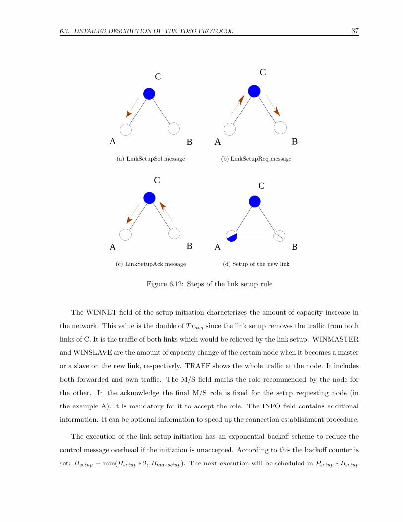
When the forwarded traffic crosses the Trminsetup value it solicits the link setup between A
and B with a LinkSetupSol message as shown in Figure 6.12a.
The link setup messages are presented in Table 6.2.
To initiate the direct connection setup node C sends a LinkSetupSol message to one of
the communicating nodes (in our case to A). When A accepts the the link setup it send a
LinkSetupReq message to B. If the link setup is beneficial for B, too, then it answers with a
LinkSetupAck.
The traffic is measured with moving average calculation. The actual value of (Tact) the traffic
is periodically added to the average value (Tavg). The exact mechanism is described in Section
7.4.
6.3. DETAILED DESCRIPTION OF THE TDSO PROTOCOL 37
A B
C
(a) LinkSetupSol message
A B
C
(b) LinkSetupReq message
BA
C
(c) LinkSetupAck message
BA
C
(d) Setup of the new link
Figure 6.12: Steps of the link setup rule
The WINNET field of the setup initiation characterizes the amount of capacity increase in
the network. This value is the double of Travg since the link setup removes the traffic from both
links of C. It is the traffic of both links which would be relieved by the link setup. WINMASTER
and WINSLAVE are the amount of capacity change of the certain node when it becomes a master
or a slave on the new link, respectively. TRAFF shows the whole traffic at the node. It includes
both forwarded and own traffic. The M/S field marks the role recommended by the node for
the other. In the acknowledge the final M/S role is fixed for the setup requesting node (in
the example A). It is mandatory for it to accept the role. The INFO field contains additional
information. It can be optional information to speed up the connection establishment procedure.
The execution of the link setup initiation has an exponential backoff scheme to reduce the
control message overhead if the initiation is unaccepted. According to this the backoff counter is
set: Bsetup = min(Bsetup ∗ 2, Bmaxsetup). The next execution will be scheduled in Psetup ∗Bsetup

38 CHAPTER 6. THE NETWORK OPTIMIZATION PROCEDURE
Order Source Destination Type of message Parameter name Parametervalue
1 C A LinkSetupSol BETWEEN A-BWINNET 380
2 A B LinkSetupReq TRAFF 190M/S SWINNET 380WINMASTER -50WINSLAVE -50
3 B A LinkSetupAck M/S SINFO
Table 6.2: Messages of the link setup
seconds where Psetup is a minimum interval between two initiations. The Tsetup value will be set
to the actual time T .
When node A receives the LinkSetupSol message it checks whether T − Tteardown < Tdown.
Tdown is the time which must elapse between two link setups. It avoids the oscillation of the
link which means the fast setup and teardown of a link periodically. Here A checks if this time
is elapsed since the last link teardown.
A calculates the GAINMASTER = WINMASTER + WINNET and
GAINSLAVE = WINSLAVE + WINNET values. The gain is the whole network gain and the
WINMASTER and WINSLAVE values are the wins of A if it would be a master or a slave on
the new link, respectively. In this case the topology modification means a capacity loss for both
A and B. The value of the loss is equal to the bridging overhead at every node. If any of the gain
values is positive then A accepts the link setup initiation and sends a LinkSetupReq message to
B (Figure 6.12b).
The LinkSetupReq contains the whole traffic of A (TRAFF) and all the win values (WIN-
NET, WINMASTER, WINSLAVE). The M/S bit indicates whether A wants to be a master or
a slave in the new link. It is set according to the greater positive gain value.
When both gains are non-positive then the link setup procedure fails.
Node B receives the LinkSetupReq and calculates its own gain values according to the fol-
lowing sums: GAINMASTER(B) = WINNET + WINMASTER(B) + WINSLAVE(A) and

6.3. DETAILED DESCRIPTION OF THE TDSO PROTOCOL 39
GAINSLAVE(B) = WINNET + WINSLAVE(B) + WINMASTER(A). B notices similar to A
whether one of the gains show that the link setup is beneficial for the network. If one of the
gains is positive then it answers to A with a LinkSetupAck message (Figure 6.12c). The M/S
value shows the role of node A in this case (which is mandatory for it). In this example the M/S
is set to M which indicates A to be the master.
At the end the new link will be set up as shown in Figure 6.12d.
6.3.2 Link master-slave switch rule
The next step of the reconfiguration will be a master-slave switch. In the previous situation the
traffic finds a shorter path and the packets will be forwarded on the new link. In this case the
packet forwarding is not efficient because A has to switch between two piconets.
It causes that A requests the role change with C in the next table check period. This decision
is based on the neighbour traffic table of A (Table 6.3).
Node Role Travg Tract Tsince Tteardown Bteardown Tswitch Bswitch
B M 190 84.67 65 - 1 - 1C S 120 0 5 - 1 76 2
Table 6.3: Neighbour traffic table of A
As an additional information we can see in the neighbour traffic table of A that the packets
are now sent to B on the direct link. The average traffic measured on the link with C will
decrease with the time.
Node A requests the role change only for link where it is a slave. It calculates its WIN as if
it would be a master. When WIN is positive then A sends a LinkMSSwitchReq message to C
as presented in Figure 6.13a. Table 6.3 shows that the last sent switch is set to the actual time
(which is 76 seconds in the example) and the backoff counter is doubled.
The messages of the master-slave switch rule are shown in Table 6.4.
The LinkMSSwitchReq message contains the WIN value and the whole traffic of the node A
(TRAFF).
Then A sets the backoff counter of the master slave switch to Bswitch = min(Bswitch ∗ 2,
Bmaxswitch). The Tswitch time is set to the actual time T . The next switch initiation will be in

40 CHAPTER 6. THE NETWORK OPTIMIZATION PROCEDURE
BA
C
(a) LinkMSSwitchReqmessage
BA
C
(b) LinkMSSwitchAckmessage
A B
C
(c) The roles arechanged
Figure 6.13: Steps of the link master-slave switch rule
Order in theexample
Source Destination Type of message Parameter name Parametervalue
4 A C LinkMSSwitchReq TRAFF 100WIN 50
5 C A LinkMSSwitchAck INFO
Table 6.4: Messages of the master-slave switch
Pswitch ∗ Bswitch seconds where Pswitch is the minimum time interval between two executions of
the master-slave switch rule.
When C receives this message it calculates its WIN (in this case its capacity loss), too. When
WIN(A) + WIN(C) > 0 (which means that the switch is beneficial for the network) it answers
with a LinkMSSwitchAck message. This answer is shown in Figure 6.13b.
At the end of the role switch procedure the roles are changed (Figure 6.13c).
6.3.3 Link teardown rule
Now the link between B and C is unnecessary because there is no traffic on it. It reduces the
available capacity for communication.
Node B checks its neighbour traffic table (Table 6.5) and notices that the traffic on the B-C
link decreased to 0. The switch between two piconets reduces the opportunity of B to receive
packets from A (bridging overhead).
First B checks whether the minimum time between setup and teardown determined by Tup

6.3. DETAILED DESCRIPTION OF THE TDSO PROTOCOL 41
is spent (Tsince + Tup < T ).
Then it calculates if the link teardown is beneficial for it. The exact calculation is as follows.
B calculates the whole capacity loss of the network WINNET= −L · Travg. Here B supposes
an alternative route with the length of 2 (L = 2). The gain of B is also calculated: GAIN
= WINNET + WIN(B) If GAIN is positive then node B sets Bteardown = min(Bteardown ∗ 2,
Bmaxteardown) backoff counter and the time Tteardown to T . Tteardown marks the time when the
last teardown request is sent.
To initiate the link teardown B sends a LinkTeardownReq message to C (see Figure 6.14a).
Node Role Travg Tract Tsince Tteardown Bteardown Tswitch Bswitch
C S 0 0 5 83 2 - 1A S 190 26.43 65 - 1 - 1
Table 6.5: Neighbour traffic table of A
A B
C
(a) LinkTeardownReqmessage
A B
C
(b) LinkTeardownAckmessage
A B
C
(c) The final piconettopology
Figure 6.14: Steps of the teardown switch rule
The link teardown messages are shown in Table 6.6.
Order in theexample
Source Destination Type of message Parameter name Parametervalue
6 A C LinkTearDownReq WIN 507 C A LinkTearDownAck INFO
Table 6.6: Messages by link teardown
The link teardown rule will be executed in B in Pteardown ∗Bteardown seconds where Pteardown

42 CHAPTER 6. THE NETWORK OPTIMIZATION PROCEDURE
is the minimum time between two teardown requests similar to the other rules.
When C receives the LinkTeardownReq message it searches for an alternative route to B.
In the example the alternative route is through A. Node C recalculates WINNET= −L · Travg
with the real L value which is 2 in this case. It also calculates GAIN = WINNET + WIN(C) +
WIN(B). When GAIN is positive it answers with a LinkTearDownAck message.
In the end a more efficient piconet is formed due to a simple reconfiguration procedure (see
Figure 6.14c).

Chapter 7
Simulation environment
I examined the methods described in Chapter 5 and 6 in simulation environment. To be able
to do measurements I modified and completed the ad hoc simulator in the PLASMA network
simulation environment [Plasma01] at Ericsson Traffic Lab.
7.1 The Bluetooth ad hoc module
The PLASMA ad hoc simulator is built up of many modules. This means that different modules
realize the base functions, the TCP/IP network protocol family or a user which generates WWW
traffic.
The ad hoc module implements a packet level simulator of the Bluetooth technology. It
includes the base functions described in the Bluetooth specification [BTspec99] like the consti-
tution of the time slots, the types of packets or the ARQ mechanism. The packet forwarding is
done by the AODV ([AODV01]) ad hoc routing protocol which operates in the IP layer. The
frequency hopping nature could lead to collisions of the packets when two piconets have the
same transmission frequency at the same moment. The physical layer contains an analytical
model to determine the packet collisions and losses. The analytical model takes the number and
traffic of the interfering piconets into account. It calculates the probability for a packet loss for
every packet.
The architecture of the ad hoc module is shown in Figure 7.1.
• The TCP object is marked with white color because I did not need to do any changes in

44 CHAPTER 7. SIMULATION ENVIRONMENT
TCP
AODV IP Switch
Manager
Scatternet
Bluetooth LL
MeasureScatternet
ManagerBluetooth LL
Measure
AODVIP Switch
TCPA
Node
B
Node
Randomwalk Space
Figure 7.1: Architecture of the PLASMA ad hoc module
this object.
• The IPSwitch implements the IP functionality in the network layer. I modified the
IPSwitch object to be able to connect it with the MANET AODV protocol implementa-
tion. All the objects filled with green (dark grey) were modified to include the scatternet
formation functions. The packet forwarding is implemented per packet which means that
the IPSwitch object sends every packet to the AODV object which determines the next hop
for that packet. Whenever the destination is unknown for the AODV object, it stores the
packet and begins a route search according to [AODV01]. When a route found message
comes from a node the AODV forwards the packet towards the next node.
• The BluetoothLL object implements the Bluetooth link layer functionalities such as logical
link setup and detach. The object includes a round-robin scheduling mechanism for intra-
piconet scheduling and a simple mechanism for inter-piconet scheduling (Section 2.3.3).
The BluetoothLL object does the segmentation and reassembly of the IP packets into
Bluetooth packets and vice versa. The object supports all packet types defined in the
specification.
• The physical layer information about the nodes are stored in the Space object. The Space

7.1. THE BLUETOOTH AD HOC MODULE 45
object calculates the packet losses caused by the frequency hopping radio channel. But as
noted in [PJohan99, Zurbes00] the effect of these losses are negligible compared to other
losses during the scatternet formation and scheduling [Racz01, NJohan99]. The radio range
of the nodes are also stored in the Space object. I assumed that there are devices with
the same radio transceiver. The Space object stores the simulation area and the positions
of the nodes and calculates the visibility for each node. These positions can be changed
due to movement which is described below. The inquiry procedure is implemented in an
abstract way. Simply every device periodically ask its visible neighbours from the Space
object.
• I implemented a random walk mobility model in the RandomWalk object. Section 7.2
explains the mobility model implementation.
• I also implemented the scatternet formation protocols in the objects Scatternet Manager
and Measure filled with light blue (light grey) color. The Scatternet Manager object
contains the implementation of both methods and the Measure object does the packet
measuring which is needed for the optimization procedure. The Scatternet Manager
implements the scatternet formation algorithm using limited broadcast of alive messages.
The object stores every connection of the node; builds up and tears down links when it is
necessary due to movement.
The Measure object measures the traffic of the node and the traffic forwarded by the node
and sends the traffic information to the Scatternet Manager object. The Scatternet
Manager object stores this information and executes the optimization rules accordingly.
An important question is how to broadcast the alive messages in the network. Since the ad
hoc routing algorithm can be implemented over the IP layer, we can exploit the properties of
the IP layer. We can send broadcast IP packets. Furthermore the usage of the IP packet format
enables us to set the TTL field of the messages. This way the limited method can be realized
easily.
In the implementation every control message is included in an IP packet and is forwarded
like a normal IP packets. This is useful because these control packets can be lost like normal IP
packet and we can observe the robustness of the scatternet formation and optimization methods.
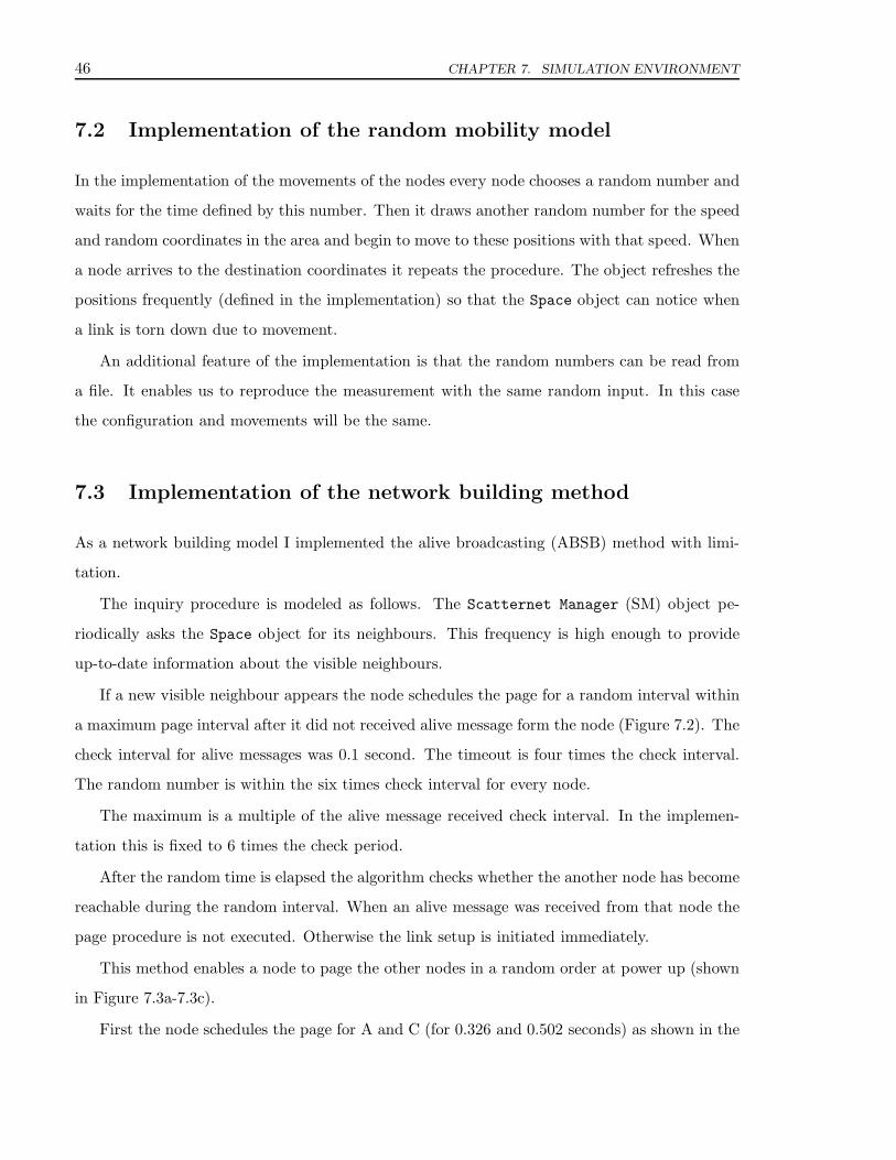
46 CHAPTER 7. SIMULATION ENVIRONMENT
7.2 Implementation of the random mobility model
In the implementation of the movements of the nodes every node chooses a random number and
waits for the time defined by this number. Then it draws another random number for the speed
and random coordinates in the area and begin to move to these positions with that speed. When
a node arrives to the destination coordinates it repeats the procedure. The object refreshes the
positions frequently (defined in the implementation) so that the Space object can notice when
a link is torn down due to movement.
An additional feature of the implementation is that the random numbers can be read from
a file. It enables us to reproduce the measurement with the same random input. In this case
the configuration and movements will be the same.
7.3 Implementation of the network building method
As a network building model I implemented the alive broadcasting (ABSB) method with limi-
tation.
The inquiry procedure is modeled as follows. The Scatternet Manager (SM) object pe-
riodically asks the Space object for its neighbours. This frequency is high enough to provide
up-to-date information about the visible neighbours.
If a new visible neighbour appears the node schedules the page for a random interval within
a maximum page interval after it did not received alive message form the node (Figure 7.2). The
check interval for alive messages was 0.1 second. The timeout is four times the check interval.
The random number is within the six times check interval for every node.
The maximum is a multiple of the alive message received check interval. In the implemen-
tation this is fixed to 6 times the check period.
After the random time is elapsed the algorithm checks whether the another node has become
reachable during the random interval. When an alive message was received from that node the
page procedure is not executed. Otherwise the link setup is initiated immediately.
This method enables a node to page the other nodes in a random order at power up (shown
in Figure 7.3a-7.3c).
First the node schedules the page for A and C (for 0.326 and 0.502 seconds) as shown in the

7.4. IMPLEMENTATION OF THE NETWORK OPTIMIZATION PROCEDURE 47
t
0 0.4 1
page to node Cpage to node A
timeout interval random page interval
Figure 7.2: Timing of the page procedure
A
B
N
C
0.326 s
time = 0 s
0.502 s
(a) Node N powers up
A
B
N
C
time = 0.326 s
(b) Page of A
A
B
N
C
time = 0.502 s
(c) Page of C
Figure 7.3: Random paging mechanism at power up
first figure. With the first page it connects to the network and receives the alive messages of
all nodes including C (see Figure 7.3b). Because C is reachable the page procedure to C is not
executed (Figure 7.3c).
The timeout is implemented as four times the alive received check period. After the fourth
check the node pages a visible neighbour when no alive message is received.
7.4 Implementation of the network optimization procedure
The TDSO protocol is implemented in two different objects. I separated the measurement tasks
and put it into the Measure object. The topology reconfiguration rules are executed by the
Scatternet Manager object.

48 CHAPTER 7. SIMULATION ENVIRONMENT
The Measure object captures every packet at the node and stores the amount of data sent
since the last averaging. Every Tcheck seconds the actual measured data is added to the average
measured traffic value with moving average calculation. The addition is done according to the
following equation:
Travg = P · Travg + (1 − P ) · Tract
T
The Travg and Tract values are the average and actual measured traffic values, respectively. P
parameter determines the weight of the old average traffic value in the new average. When P is
low the average quickly follows the actual traffic value. When P converges to 1 then the average
traffic follows the actual traffic slower. T means the time when the averaging is executed.
The reaction speed of the algorithm is affected by the P and Tcheck parameters. I set P near
to 0.01 to make the protocol reactions fast. In this case the reaction speed depends only on the
Tcheck value. I investigate this dependence in Section 8.2.1.
The protocol executes the rules independently from each other. The rules are executed for
every link periodically. The execution time is determined by the Texecution parameter. This is
presented in Section 8.2.2.
The link setup is affected by the parameter Trminsetup, the minimum traffic needed for link
setup. In my implementation I fixed this parameter to 200 kbit/s. This is an arbitrarily chosen
value. Further investigations are possible in the future.
The bridging means an overhead for the communication. I used a simplified model for the
bridging overhead. The Boverhead value was 50 kbit/s which marks the capacity reduction for ev-
ery additional piconet membership . The Boverhead value is strongly dependent on the scheduling
algorithm (my scheduling algorithm implementation is presented in the next section). According
to this scheduling algorithm or the traffic of the neighbouring piconets the bridging overhead
could be calculated more accurately. This is an important topic for future investigations.
7.5 Scheduling implementation
I implemented a simple scheduling algorithm in the ad hoc module.
According to the algorithm every node spends an amount of time in its own piconet when it
is a master. During its residence it allows every slave to send data to it.
When the node is member of more then one piconet then it switches to a foreign piconet

7.5. SCHEDULING IMPLEMENTATION 49
after all of its slaves were solicited. In the foreign piconet the node waits till the master of that
piconet allows it to send data.
Afterwards it switches back to its own piconet and begins to poll its slaves again. When
the node is member of more piconets then it changes to every piconet based on a round-robin
scheme.
This scheduling mechanism is a simple solution for Bluetooth scheduling. A more efficient
method is presented in [Racz01].

Chapter 8
Results of the simulation
In this chapter I present simulation results related to the limited ABSB and TDSO protocols.
First I give examples for the piconet and scatternet building procedures (Section 8.1). Then I
explain how the protocol works when the nodes tune the limitation for the alive message sending
(Section 8.1.3).
After the investigations of the scatternet building methods I present initial simulation results
of the TDSO protocol in Section 8.2.
8.1 Investigations of the ABSB protocol
To evaluate the correct working of the alive broadcasting method I built up a scatternet from 3
and 5 nodes.
8.1.1 Piconet building with ABSB
First there were 3 nodes which were located in a fixed area. The simulation area was a square
with a side length of 12. This length provides an area where there is a great chance for the
nodes to form a scatternet. It is also possible for links to break which is necessary to the ABSB
protocol evaluation.
To measure the capacity of the network I used a TCP flow between the nodes A and B. The
TCP traffic used the maximum available capacity of the network. The TCP traffic was modeled
as a sending of a infinitely long file.
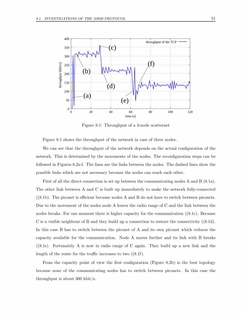
8.1. INVESTIGATIONS OF THE ABSB PROTOCOL 51
0
50
100
150
200
250
300
350
400
0 20 40 60 80 100 120
thro
ughp
ut (
kbit/
s)
time (s)
throughput of the TCP
(c)
(d)
(e)
(f)
(a)
(b)
Figure 8.1: Throughput of a 3-node scatternet
Figure 8.1 shows the throughput of the network in case of three nodes.
We can see that the throughput of the network depends on the actual configuration of the
network. This is determined by the movements of the nodes. The reconfiguration steps can be
followed in Figures 8.2a-f. The lines are the links between the nodes. The dashed lines show the
possible links which are not necessary because the nodes can reach each other.
First of all the direct connection is set up between the communicating nodes A and B (8.1a).
The other link between A and C is built up immediately to make the network fully-connected
((8.1b). The piconet is efficient because nodes A and B do not have to switch between piconets.
Due to the movement of the nodes node A leaves the radio range of C and the link between the
nodes breaks. For one moment there is higher capacity for the communication ((8.1c). Because
C is a visible neighbour of B and they build up a connection to restore the connectivity ((8.1d).
In this case B has to switch between the piconet of A and its own piconet which reduces the
capacity available for the communication. Node A moves further and its link with B breaks
((8.1e). Fortunately A is now in radio range of C again. They build up a new link and the
length of the route for the traffic increases to two ((8.1f).
From the capacity point of view the first configuration (Figure 8.2b) is the best topology
because none of the communicating nodes has to switch between piconets. In this case the
throughput is about 300 kbit/s.

52 CHAPTER 8. RESULTS OF THE SIMULATION
A B
C
(a) time = 0.42 s
A B
C
(b) time = 0.55 s
A B
C
(c) time = 28.48 s
A B
C
(d) time = 29.29s
A B
C
(e) time = 65.48 s
A B
C
(f) time = 66.29 s
Figure 8.2: Topology reconfigurations in the 3-node scatternet
There are three aspects which determine the maximum throughput.
• TCP/IP overhead: The throughput measured is the user throughput of the TCP com-
munication. The whole TCP/IP throughput which is carried on the Bluetooth network
includes the TCP and IP packet headers, too. It includes the acknowledgments of the
TCP packets.
• Polling of the other node: Despite the lack of communication with the node C node A has
to poll node C as well. It has to check whether node C has to send something.
• Whole bridging overhead along the communication path. This value is determined by the
single bridging overhead values at each node as described in Section 2.3.3. The whole
bridging overhead also depends on the length of the path.
At 28.48 seconds the link between A and C breaks which enables a little more capacity for
the traffic (see Figure 8.2c). This is because A does not have to poll the node C. After that the
new link reduces the throughput with the bridging overhead of B (as shown in Figure 8.2d).

8.1. INVESTIGATIONS OF THE ABSB PROTOCOL 53
When the direct link breaks and the communication path increases to two, the throughput
reduces further (Figure 8.2f) to about 130 kbit/s. This can be explained with the increase of
the communication path and the fact that node C is a slave in both piconets. Node C has to
wait in both piconets to be polled.
8.1.2 Scatternet building with ABSB
The similar throughput is shown in Figure 8.3 however with a scatternet of 5 nodes.
0
50
100
150
200
250
300
0 50 100 150 200
thro
uhgp
ut (
kbit/
s)
time (s)
throughput of the TCP
Figure 8.3: Throughput of a scatternet with 5 nodes
The simulation area was 20x20 square in this case. The exact topology reconfiguration
procedure is shown in Appendix A. The scope of the ABSB protocol was 4.
In case of a scatternet with more nodes the chance for link break is higher. We can see in the
figure that the communication stops many times. The building algorithm is able to reconnect
the nodes when they are in visibility range to each other. We can also see that the throughput
is about 120 kbit/s for the most time. This is caused by the great chance for bridging overhead
and the long path of the data flow.
8.1.3 Increasing the limit of the messaging
Let us examine how the value of the scope affects the TCP throughput.

54 CHAPTER 8. RESULTS OF THE SIMULATION
I simulated a network with 6 nodes in an area of 15x15 meters. I increased the scope of the
limited ABSB protocol from 2 to 5 (Figure 8.4).
0
20
40
60
80
100
120
2 3 3.5 4 4.5 52.5
limit of Alive message sending
thro
ughp
ut (
kbit/
s)
TCP throughputalive message overhead
Figure 8.4: The throughput and alive message overhead increasing the scope
In the figure the line shows the trend of the change of TCP throughput. As we can see the
carried traffic of the network decreases with the higher scope value.
This can be explained with the fact that in case of a low scope value more redundant
connections will be built up. This redundancy enables the routing algorithm to find a shorter
path in the network between the communicating nodes. The fewer is the redundancy the longer
is the path of the communication. A longer route means more bridging in the network which
decreases the TCP throughput. This problem can be solved with the TDSO protocol.
We can also point out that the average control message overhead generated by the alive
messages does not increase with the limit value. When there are fewer links in the network
the nodes have to send fewer alive messages. It decreases the total amount of alive messages
sent. The other effect is that the higher the scope value the further are the alive messages sent
in the network. This effect increases the amount of alive messages in the whole network. The
two effects are in balance with each other. This can be a possible explanation for the results of
Figure 8.4.
As a consequence it is useful to choose a low limit value for the building protocol when there

8.2. SIMULATION RESULTS OF THE TDSO PROTOCOL 55
is no scatternet optimization. However we must also take other aspects into account such as
scheduling and routing in a redundant connected network.
8.2 Simulation results of the TDSO protocol
In this section I describe my initial investigations regarding the TDSO protocol. In the following
I present the algorithm reaction speed which depends on the parameters Tcheck and Texecution.
To be able to examine the features of the TDSO protocol I separated it from the ABSB
protocol. I simulated a simple piconet configuration which is presented in Figure 8.5.
A : 100 kb/sC B
B
C
A
Traffic :
Figure 8.5: A simple piconet topology
I simulated a simple reconfiguration procedure according to the example in Section 6.2.1.
The TCP source was the same as in the case of the scatternet building procedure. The
execution of the rules began at 60 seconds. This was needed to let the TCP mechanism stay at
a constant average transmission rate.
8.2.1 Effect of the Tcheck value
I first examined the effect of the Tcheck parameter which determines how often the nodes refresh
the measured traffic information (Section 7.4). The more frequent the refresh procedure is the
faster the node can react to traffic changes. I measured the TCP throughput by two different
Tcheck values. The results are presented in Figures 8.6a and b. The begin and end of the piconet
reconfiguration is presented with an arrow in the figures.
The value of the Texecution parameter was 1 second in both cases.
When we choose a low value for Tcheck then the rules will be executed according to an actual
traffic value. In Figure 8.6a this value is one which means a relative frequent averaging. In this
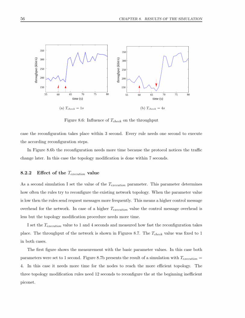
56 CHAPTER 8. RESULTS OF THE SIMULATION
150000
200000
250000
300000
350000
55 60 65 70 75 80
thro
ughp
ut [
kb/s
]
time [s]
150
200
250
300
350
6055 65 70 75 80
time (s)
thro
ughp
ut (
kbit/
s)
(a) Tcheck = 1s
150000
200000
250000
300000
350000
55 60 65 70 75 80
thro
ughp
ut [
kb/s
]
time [s]
150
55
200
250
300
350
60 65 70 75 80
time (s)
thro
ughp
ut (
kbit/
s)
(b) Tcheck = 4s
Figure 8.6: Influence of Tcheck on the throughput
case the reconfiguration takes place within 3 second. Every rule needs one second to execute
the according reconfiguration steps.
In Figure 8.6b the reconfiguration needs more time because the protocol notices the traffic
change later. In this case the topology modification is done within 7 seconds.
8.2.2 Effect of the Texecution value
As a second simulation I set the value of the Texecution parameter. This parameter determines
how often the rules try to reconfigure the existing network topology. When the parameter value
is low then the rules send request messages more frequently. This means a higher control message
overhead for the network. In case of a higher Texecution value the control message overhead is
less but the topology modification procedure needs more time.
I set the Texecution value to 1 and 4 seconds and measured how fast the reconfiguration takes
place. The throughput of the network is shown in Figures 8.7. The Tcheck value was fixed to 1
in both cases.
The first figure shows the measurement with the basic parameter values. In this case both
parameters were set to 1 second. Figure 8.7b presents the result of a simulation with Texecution =
4. In this case it needs more time for the nodes to reach the more efficient topology. The
three topology modification rules need 12 seconds to reconfigure the at the beginning inefficient
piconet.
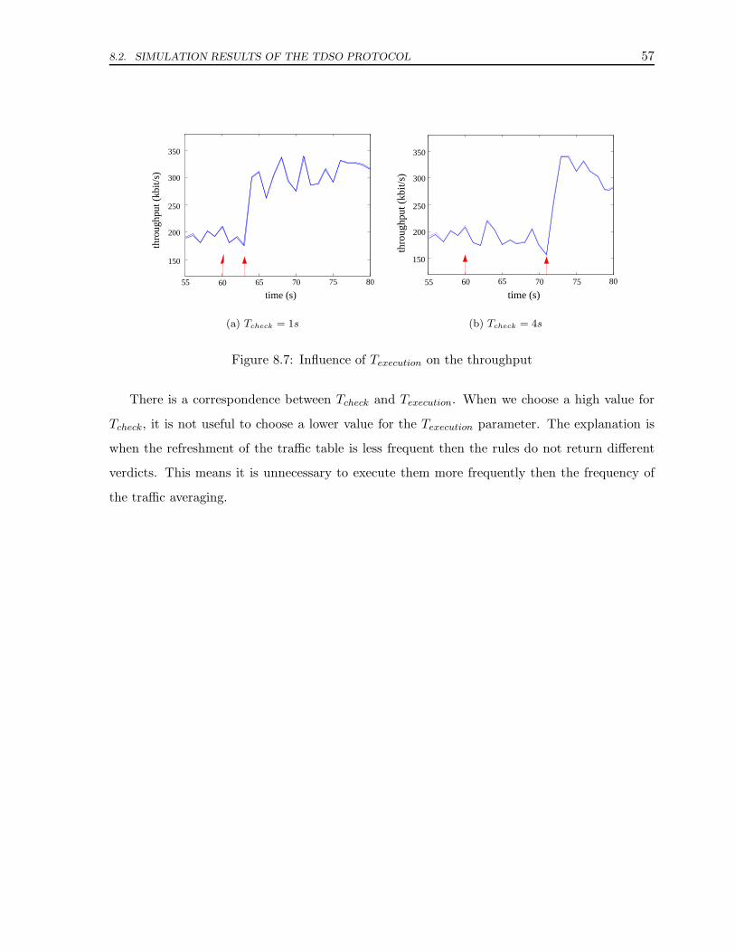
8.2. SIMULATION RESULTS OF THE TDSO PROTOCOL 57
150000
200000
250000
300000
350000
55 60 65 70 75 80
thro
ughp
ut [
kb/s
]
time [s]
150
200
250
300
350
6055 65 70 75 80
time (s)
thro
ughp
ut (
kbit/
s)
(a) Tcheck = 1s
150000
200000
250000
300000
350000
55 60 65 70 75 80
thro
ughp
ut [
kb/s
]
time [s]
150
200
250
300
350
55 60 65 70 75 80
time (s)
thro
ughp
ut (
kbit/
s)
(b) Tcheck = 4s
Figure 8.7: Influence of Texecution on the throughput
There is a correspondence between Tcheck and Texecution. When we choose a high value for
Tcheck, it is not useful to choose a lower value for the Texecution parameter. The explanation is
when the refreshment of the traffic table is less frequent then the rules do not return different
verdicts. This means it is unnecessary to execute them more frequently then the frequency of
the traffic averaging.

Chapter 9
Summary
In my thesis I have presented the Bluetooth wireless technology. This short-range radio technol-
ogy is able to replace the cables between the devices. In addition, the Bluetooth specification
enables the formation of larger networks. This network is called scatternet.
However the Bluetooth specification does not define how to form a larger network. I have
considered this problem and split it up into 3 different parts.
• connection setup mechanism
• scatternet building and maintenance
• scatternet optimization
In my thesis I addressed the problems of scatternet building and scatternet optimization.
I have designed two alternative protocols for the scatternet building and maintenance prob-
lem. One of the solutions uses periodic broadcasting of alive messages (ABSB method). The
messages advertise the presence of the node in the network. When a node does not receive any
alive message from another node which is within radio range then it builds up a direct connec-
tion. The other protocol is based on the topology information messages of the routing algorithm
(RBSB method). When a node does not find a route to another node then it builds up a direct
connection when they are visible to each other. I have presented an extension to both methods
which uses limited message sending.
The suggested methods solve network building and maintenance, but the traffic may be
forwarded in an inefficient route. It is useful to reconfigure the fully-connected network topology

59
into a more efficient one. I have designed a scatternet optimizer protocol (TDSO) to solve
this problem. This procedure reconfigures the topology according to local measured traffic
information. Based on this information every node executes 3 simple rules to build up and
release connections and change the master-slave roles if it is useful. Each rule increases the local
efficiency and so the whole network capacity is improved.
All three protocols are distributed solutions. Every node executes rules according to local
information. The rules are executed periodically and independently from each other.
I have implemented the methods in the ad hoc simulator of the PLASMA simulation envi-
ronment. I implemented the protocols in the Scatternet Manager object. Furthermore I have
implemented a random walk mobility model.
The simulation results of the alive broadcasting method showed that the protocol is able to
build up a fully-connected network and keep it connected during the movement of the nodes.
When I increased the scope of the protocol the throughput decreased. This occured because the
traffic was forwarded on a longer route. The increasing of the limit does not affect the average
amount of overhead generated by the alive messages.
I simulated the scatternet optimizer method from the scatternet builder. The simulations
pointed out that the protocol is tunable by two main parameters Tcheck and Texecution. The
lower were the parameter values the faster was the reconfiguration of the network.
The simulation showed that the network formation protocols were able to form a Bluetooth
ad hoc network and reconfigure it into a more efficient one.
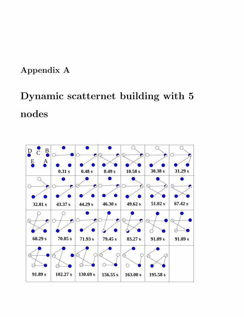
Appendix A
Dynamic scatternet building with 5
nodes
B
A
D
E
C
195.58 s
70.85 s68.29 s
67.42 s51.02 s49.62 s46.30 s44.29 s43.37 s32.81 s
31.29 s30.38 s10.58 s0.49 s0.48 s0.31 s
71.93 s 79.45 s 83.27 s 91.09 s 91.89 s
91.89 s 102.27 s 130.69 s 156.55 s 163.00 s

In the network node A communicates with B. The TCP communication uses the maximum
available capacity.
As a first step the nodes build up the full connected network. Node C is out of range till the
10th second. At about 30 seconds the communication stops because node A moves out from the
range of D. To reconnect node B builds up a link to A. However there is a direct link between the
communicating nodes. Now the throughput does not increase because node B is member in 3
piconets. The bridging overhead decreases its capacity to about 100 kbit/s. The communication
can continue from 51 seconds. The configuration is similar to the one at the beginning one.
Node A moves out from the range of all network members during the interval from 70 and 83
seconds. The communication continues at 130 seconds and the throughput will be higher when
unnecessary link of A break.
The link modification log file of the program is shown below:
0.31285 .scatman2 (ScatBuilderBroad): oooo Flow Setup(flowid,between[0,1]): 1,64,66 oooo
0.48148 .scatman0 (ScatBuilderBroad): oooo Flow Setup(flowid,between[0,1]): 3,62,64 oooo
0.49014 .scatman1 (ScatBuilderBroad): oooo Flow Setup(flowid,between[0,1]): 5,63,66 oooo
10.58843 .scatman2 (ScatBuilderBroad): oooo Flow Setup(flowid,between[0,1]): 8,64,65 oooo
30.38216 .scatman4 (ScatBuilderBroad): oooo Flow Release(flowid,between[0,1]): 5,63,66 oooo
31.29000 .scatman1 (ScatBuilderBroad): oooo Flow Setup(flowid,between[0,1]): 10,63,64 oooo
32.81088 .scatman2 (ScatBuilderBroad): oooo Flow Release(flowid,between[0,1]): 10,63,64 oooo
43.37250 .scatman3 (ScatBuilderBroad): oooo Flow Release(flowid,between[0,1]): 8,64,65 oooo
44.29000 .scatman3 (ScatBuilderBroad): oooo Flow Setup(flowid,between[0,1]): 11,65,66 oooo
46.30065 .scatman4 (ScatBuilderBroad): oooo Flow Release(flowid,between[0,1]): 11,65,66 oooo
49.62628 .scatman3 (ScatBuilderBroad): oooo Flow Setup(flowid,between[0,1]): 13,65,64 oooo
51.02427 .scatman1 (ScatBuilderBroad): oooo Flow Setup(flowid,between[0,1]): 15,63,66 oooo
67.47086 .scatman2 (ScatBuilderBroad): oooo Flow Release(flowid,between[0,1]): 13,65,64 oooo
68.29000 .scatman0 (ScatBuilderBroad): oooo Flow Setup(flowid,between[0,1]): 16,62,65 oooo
70.85032 .scatman4 (ScatBuilderBroad): oooo Flow Release(flowid,between[0,1]): 15,63,66 oooo
71.93126 .scatman3 (ScatBuilderBroad): oooo Flow Release(flowid,between[0,1]): 16,62,65 oooo
79.44898 .scatman3 (ScatBuilderBroad): oooo Flow Setup(flowid,between[0,1]): 17,65,62 oooo
83.26891 .scatman1 (ScatBuilderBroad): oooo Flow Setup(flowid,between[0,1]): 19,63,66 oooo
91.09126 .scatman2 (ScatBuilderBroad): oooo Flow Release(flowid,between[0,1]): 3,62,64 oooo
91.89000 .scatman1 (ScatBuilderBroad): oooo Flow Setup(flowid,between[0,1]): 20,63,62 oooo
91.89000 .scatman3 (ScatBuilderBroad): oooo Flow Setup(flowid,between[0,1]): 22,65,66 oooo
102.27062 .scatman4 (ScatBuilderBroad): oooo Flow Release(flowid,between[0,1]): 1,64,66 oooo
130.69284 .scatman1 (ScatBuilderBroad): oooo Flow Setup(flowid,between[0,1]): 24,63,64 oooo
156.55319 .scatman0 (ScatBuilderBroad): oooo Flow Release(flowid,between[0,1]): 17,65,62 oooo
163.00208 .scatman0 (ScatBuilderBroad): oooo Flow Release(flowid,between[0,1]): 20,63,62 oooo
195.58463 .scatman0 (ScatBuilderBroad): oooo Flow Setup(flowid,between[0,1]): 25,62,64 oooo

References
[AODV01] C. E. Perkins and E. M. Royer: “Ad-hoc On-Demand Distance Vector Routing”,Proceedings of 2nd IEEE Workshop on Mobile Computing Systems and Applica-tions, February 1999. orhttp://www.ietf.org/internet-drafts/draft-ietf-manet-aodv-08.txt, March 2001
[BTspec99] Bluetooth Baseband Specification version 1.0 B, November 1999,http://www.bluetooth.com/
[Dante21] Dante Alighieri: “La Divina Commedia (The Divine Comedy)”, Venice 1321
[Dijkstra59] E. Dijkstra: “A Note Two Problems in Connection with Graphs”, NumerischeMathematic, vol.1, pp. 269-271, 1959
[DSDV94] C. Perkins and P Bhagwat: “Highly Dynamic Destination-sequenced DistanceVector Routing (DSDV) for mobile computers”, in ACM SIGCOMM, October1994
[DSR01] David B. Johnson and David A. Maltz: “Dynamic Source Routing in Ad HocWireless Networks” In Mobile Computing, edited by Tomasz Imielinski and HankKorth, Chapter 5, pages 153-181, Kluwer Academic Publishers, 1996. orJ. Broch, D. B. Johnson, D. A. Maltz: “The Dynamic Source Routing Protocolfor Mobile Ad Hoc Networks”, IETF Internet Draft draft-ietf-manet-dsr-05.txt,March 2001
[Haartsen98] Jaap Haartsen: “Bluetooth - The universal radio interface for ad hoc, wirelessconnectivity”, Ericsson Review No.3, 1998, pp. 110-117
[Haas01] Z. J. Haas, M. R. Pearlman, P. Samar: “The Intrazone Routing Protocol (IARP)for Ad Hoc Networks”, draft-ietf-manet-zone-iarp-00.txt, January 2001
[Imre00] dr. Imre Sandor: “Bevezetes a mobil szamıtastechnikaba”(Introduction to MobileComputing),http://www.hit.bme.hu/mcl/hu/oktatas.html, 2000
[IrDA01] Patrick J. Megowan, David W. Suvak, Charles D. Knutson: “IrDA In-frared Communications: An Overview”, Counterpoint Systems Foundry, Inc.,http://www.irda.org
[MANET01] Mobile Ad-hoc Networks Working Group of IETF,http://www.ietf.org/html.charters/manet-charter.html
[Miklos00] Gy. Miklos: “Bluetooth: Olcso, drotnelkuli helyi osszekottetes”, (“Bluetooth:Cheap, wireless local connectivity”), Magyar Tavkozles, September 2000
[NJohan99] N. Johansson, U. Korner, P. Johansson: “Performance Evaluation of SchedulingAlgorithms for Bluetooth”, Proceedings of IFIP TC6 Fifth International Confer-ence on Broadband Communications’99, Hong-Kong, November 10-12, 1999.
[OLSR00] P.Jaquet, P. Muhlethaler, A Qayyum: “Optimized Link State Routing Protocol(OLSR)”, draft-ietf-manet-olsr-03.txt, November 2000
[Parkinson95] B. W. Parkinson and J. J. Spilker Jr. (eds.), “Global Positioning System: Theoryand Applications”, Vols. 1-2, Am. Inst. of Aeronautics and Astronautics, 1995.
[Pearlman99] M. R. Pearlman and Z. J. Haas: “Determining the Optimal Configuration of forthe Zone Routing Protocol”, IEEE JSAC, special issue on Ad-Hoc Networks, vol.17, no.8, August 1999
[Pei00] G. Pei, M. Gerla, X. Hong, T. W. Chen: “Fisheye State Routing Protocol (FSR)for Ad hoc Networks”, draft-ietf-manet-fsr-00.txt, November 2000
[PJohan99] P. Johansson, N. Johansson, U. Korner, J. Elg, G. Svennarp: “Short Range RadioBased Ad-hoc Networking: Performance and Properties”, Proceedings of ICC’99,Vancouver, 1999.
[Plasma01] “PLASMA CORE Programmer’s Guide”, 2001
[Racz00] Gy. Miklos, A. Racz, Z. Turanyi, A. Valko, P. Johansson: “Performance Aspectsof Bluetooth Scatternet Formation”, MobiHOC (First IEEE Annual Workshop onMobile Ad Hoc Networking and Computing), August 2000, The submission wasaccepted as a poster.
[Racz01] A. Racz, Gy. Miklos, F. Kubinszky, A. Valko: “A Pseudo Random CoordinatedScheduling Algorithm for Bluetooth Scatternets” MobiHOC, The ACM Sympo-sium on Mobile Ad Hoc Networking and Computing October 4-5, 2001, LongBeach, California, USA, submitted paper
[Raman01] B. Raman, P. Bhagwat, S. Seshan: “Arguments for Cross-Layer Optimization inBluetooth Scatternets” Symposium on Applications and the Internet (SAINT’01),Jan 2001
[Roman01] G. C. Roman, Q. Huang, A. Hazemi: “Consistent Group Membership in AdHoc Networks”, In Proceedings of the 23rd International Conference in SoftwareEngineering (ISCE), Toronto, Canada, May 2001.
[Salonidis01] T. Salonidis, P. Bhagwat, L. Tassiulas, R. LaMaire: “Proximity Awareness andAd Hoc Network Establishment in Bluetooth”, Technical Report, February 2001,http://www.isr.umd.edu/CSHCN/
[Stevens94] R. W. Stevens: “TCP/IP Illustrated Volume 1: The Protocols”, Addison-Wesley,1994.

[Tannen96] A. S. Tannenbaum: “Computer Networks”, Prentice Hall, Englewood Cliffs, 3rdedition, 1996
[WLAN99] J. T. Geier: “Wireless LANs. Implementing Interoperable Networks”, MacmillanTechnical Publishing, pp. 89-125, 1999, ISBN 1-57870-081-7.
[Zurbes00] S. Zurbes, W. Stahl, K. Matheus, J. Haartsen: “Radio Network Performance ofBluetooth”, Proceedings of ICC’2000, New Orleans, 18-22 June, 2000.