Blow-up of regular submanifolds in Heisenberg

groups and applications

Valentino Magnani

Pisa University,Department of Mathematics,

Largo Bruno Pontecorvo 5, I-56127, Pisa, Italye-mail magnani@dm.unipi.it

Abstract

We obtain a blow-up theorem for regular submanifolds in the Heisenberggroup, where intrinsic dilations are used. Main consequence of this result is anexplicit formula for the density of (p+1)-dimensional spherical Hausdor� measurerestricted to a p-dimensional submanifold with respect to the Riemannian surfacemeasure. We explicitly compute this formula in some simple examples and wepresent a lower semicontinuity result for the spherical Hausdor� measure withrespect to the weak convergence of currents. Another application is the proof ofan intrinsic coarea formula for vector-valued mappings on the Heisenberg group.

Contents

1 Introduction 2

2 Some basic notions 4

3 Blow-up at transverse points 9

4 Spherical Hausdor� measure of submanifolds 16

5 Coarea formula 23

Mathematics Subject Classi�cation: 28A75 (22E25)Keywords: Heisenberg group, Hausdor� measure,coarea formula

1

1 Introduction

In recent years, several e�orts have been devoted to the project of developing Analysisand Geometry in strati�ed groups and more general Carnot-Carath�eodory spaces withseveral monographs and surveys on this subject. Among them we mention [3], [6], [13],[16], [23], [28], but this list could be surely enlarged.

Our study �ts into the recent project of developing Geometric Measure Theoryin these spaces. Ambient of our investigations is the (2n+1)-dimensional HeisenberggroupHn, which represents the simplest model of non-Abelian strati�ed group, [6], [27].Aim of this paper is to present an intrinsic blow-up theorem for C1 submanifolds in thegeometry of the Heisenberg group along with its applications. The main feature of thisprocedure is the use of natural dilations of the group, namely, a one-parameter family ofgroup homomorphisms that are homogeneous with respect to the distance of the group.Recall that dilations in Hn are anisotropic, hence they di�erently act on di�erentdirections of the submanifold. The foremost directions are the so-called horizontaldirections, that determine the \sub-Riemannian geometry" of the Heisenberg group:at any point x 2 Hn a 2n-dimensional subspace HxH

n � TxH2n+1 is given and the

family of all horizontal spaces HxHn forms the so-called horizontal subbundle HHn.

We will defer full de�nitions to Section 2.The blow-up procedure consists in enlarging the submanifold � at some point x 2 �

by intrinsic dilations and taking the intersection of the magni�ed submanifold with abounded set centered at x. We are interested in studying the case when Tx� 6� HxH

n,namely, x is a transverse point. The e�ect of rescaling the submanifold at a transversepoint x can be obtained by considering the behavior of volp(Bx;r \�)=r

p+1 as r ! 0+,that heuristically is

volp(Bx;r \ �)

rp+1=

volp(lx�r(B1 \ �x;r))rp+1

=volp(�r(B1 \ �x;r))

rp+1� �(x) volp(B1 \ �x;r):

Here volp denotes the p-dimensional Riemannian measure restricted to �, the lefttranslation lx : Hn �! H

n is given by lx(y) = x � y, the dilation of factor r > 0is �r : Hn �! H

n, the dilated submanifold at x is �x;r = �1=r(lx�1�) and Bx;r isthe open ball of center x and radius r with respect to a �xed homogeneous distance.The meaning of �(x) will be clear in the following theorem, that makes rigorous ourprevious consideration and represents our �rst main result.

Theorem 1.1 (Blow-up) Let � be a p-dimensional C1 submanifold of , where is an open subset of Hn and let x be a transverse point. Then the following limit holds

limr!0+

volp(� \Bx;r)

rp+1=��p(��;V(x))j��;V(x)j

: (1)

A novel object appearing in this limit is the vertical tangent p-vector ��;V(x), intro-duced in De�nition 2.13. Its associated p-dimensional subspace of hn is a subalgebra

2

whose image through the exponential map represents the blow-up limit of the rescaledsubmanifold �x;r as r ! 0+. The p-vector ��;V(x) in higher codimension plays thesame role that the well known horizontal normal �H plays in codimension one (comparefor instance with [19]). The metric factor �(��;V(x)), introduced in [19], correspondsto the measure of the intersection of B1 with the vertical subspace associated to thevertical tangent p-vector ��;V(x). A �rst consequence of Theorem 1.1 is an explicit for-mula to compute the (p+1)-dimensional spherical Hausdor� measure of p-dimensionalC1 submanifolds in the Heisenberg group. In fact, thanks to Sp+1-negligibility ofcharacteristic points proved in [22], Theorem 1.1 along with standard theorems ondi�erentation of measures, immediately give the following result.

Theorem 1.2 Let � be a homogeneous distance with constant metric factor � > 0and let Sp+1

Hn= �Sp+1� . Then we have

Sp+1Hn

(�) =

Z�j��;V(x)j dvolp(x): (2)

Note that in codimension one, the integral formula (2) �ts into the results of [19] instrati�ed groups. The connection between these results is shown in Proposition 4.15.There are several examples of homogeneous distances satisfying hypothesis of Theo-rem 1.2, as we show in Example 4.6. Proposition 4.5 shows a class of homogeneousdistances having constant metric factor. Proposition 4.7 shows how the computationof the (p+1)-dimensional spherical Hausdor� measure of a submanifold can be easilyperformed in several examples, that will appear in Section 4.

Another consequence of Theorem 1.1 is the validity of an intrinsic coarea formulafor vector-valued Lipschitz mappings de�ned on the Heisenberg group. By Sard theo-rem and the classical Whitney approximation theorem we can assume that a.e. levelset is a submanifold of class C1, then we apply representation formula (2). The coreof the proof stands in the key relation

j��;V(x)j =JHf(x)

Jgf(x); (3)

which surprisingly connects vertical tangent p-vector with horizontal jacobian JHf .The proof of (3) is given in Theorem 3.3. Thus, we can establish the following result.

Theorem 1.3 (Coarea formula) Let f : A �! Rk be a Riemannian Lipschitz map,

where A � Hn is a measurable subset and 1 � k < 2n + 1. Let � be a homogeneous

distance with constant metric factor � > 0. Then for every measurable function u :A �! [0;+1] the formulaZ

Au(x) JHf(x) dx =

ZRk

Zf�1(t)\A

u(y) dSp+1Hn

(y)

!dt (4)

holds, where p = 2n+ 1� k and Sp+1Hn

= �Sp+1� .

3

This coarea formula along with that of [21], which is a particular case, represent�rst examples of intrinsic coarea formulae for vector valued mappings de�ned on non-Abelian Carnot groups. It remains an interesting open question the extension of coareaformula to Lipschitz mappings with respect to a homogeneous distance. Only in thecase of real-valued mappings this problem has been settled in [20]. This questionis intimately related to a blow-up theorem of \intrinsicly regular" submanifolds. Inthis connection, we mention a recent work by Franchi, Serapioni and Serra Cassano[10], where a notion of intrinisic submanifold in Hn has been introduced in arbitrarycodimension. According the their terminology, a k-codimensional H-regular subman-ifold for algebraic reasons must satisfy 1 � k � n. With this restriction it might behighly irregular, even unrecti�able in the Euclidean sense, [14]. Nevertheless they showthat an area-type formula for its (p+1)-dimensional spherical Hausdor� measure stillholds. Here we wish to emphasize the di�erence in our approach, where we considerC1 submanifolds, but with no restriction on their codimension.

Let us summarize the contents of the present paper. Section 2 recalls some no-tions. Section 3 is devoted to the proof of Theorem 1.1. In Section 4 we show thevalidity of Theorem 1.2, along with its applications. In Proposition 4.5, we single outa privileged class of homogeneous distances having constant metric factor. We presentseveral explicit computations of (p+1)-dimensional spherical Hausdor� measure inconcrete examples. As another application of Theorem 1.2, we show a lower semicon-tintuity result for the spherical Hausdor� measure with respect to weak convergenceof regular currents. Section 5 establishes an intrinsic coarea formula for vector-valuedRiemannian Lipschitz mappings on the Heisenberg group.

Acknowledgments. I wish to thank Bruno Franchi, Raul Serapioni and FrancescoSerra Cassano for pleasant discussions on intrinsic surface area in Heisenberg groups.

2 Some basic notions

The (2n+1)-dimensional Heisenberg group Hn is a simply connected Lie group whoseLie algebra hn is equipped with a basis (X1; : : : ; X2n; Z) satisfying the bracket relations

[Xk; Xk+n] = 2Z (5)

for every k = 1; : : : ; n. We will identify the Lie algebra hn with the isomorphic Liealgebra of left invariant vector �elds on Hn, so that any Xj also denotes a left in-variant vector �eld of Hn. In the terminology of Di�erential Geometry, the basis(X1; : : : ; X2n; Z) forms a moving frame in Hn. We will say that (X1; : : : ; X2n; Z) isour standard frame. In particular, (X1; : : : ; X2n) is a horizontal frame and it spansa smooth distribution of 2n-dimensional hyperplanes, called horizontal hyperplanes

and denoted by HxHn for every x 2 H

n. The collection of all horizontal hyper-planes forms the so called horizontal subbundle, denoted by HHn. In the sequel, we

4

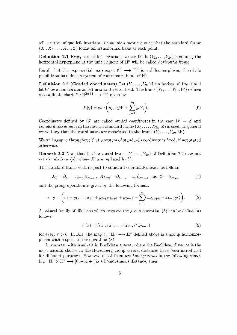
will �x the unique left invariant Riemannian metric g such that the standard frame(X1; X2; : : : ; X2n; Z) forms an orthonormal basis at each point.

De�nition 2.1 Every set of left invariant vector �elds (Y1; : : : ; Y2n) spanning thehorizontal hyperplane at the unit element of Hn will be called horizontal frame.

Recall that the exponential map exp : hn �! Hn is a di�eomorphism, then it is

possible to introduce a system of coordinates in all of Hn.

De�nition 2.2 (Graded coordinates) Let (Y1; : : : ; Y2n) be a horizontal frame andletW be a non horizontal left invariant vector �eld. The frame (Y1; : : : ; Y2n;W ) de�nesa coordinate chart F : R2n+1 �! H

n given by

F (y) = exp

�y2n+1W +

2nXj=1

yjYj

�: (6)

Coordinates de�ned by (6) are called graded coordinates in the case W = Z andstandard coordinates in the case the standard frame (X1; : : : ; X2n; Z) is used. In generalwe will say that the coordinates are associated to the frame (Y1; : : : ; Y2n;W )

We will assume throughout that a system of standard coordinate is �xed, if not statedotherwise.

Remark 2.3 Note that the horizontal frame (Y1; : : : ; Y2n) of De�nition 2.2 may notsatisfy relations (5), where Xi are replaced by Yi.

The standard frame with respect to standard coordinates reads as follows

~Xk = @xk � xk+n @x2n+1 ;~Xk+n = @xk+n + xk @x2n+1 and ~Z = @x2n+1 (7)

and the group operation is given by the following formula

x � y =

�x1 + y1; : : : ; x2n + y2n; x2n+1 + y2n+1 +

nXj=1

(xkyk+n � xk+nyk)

�: (8)

A natural family of dilations which respects the group operation (8) can be de�ned asfollows

�r(x) = (rx1; rx2; : : : ; rx2n; r2x2n+1) (9)

for every r > 0. In fact, the map �r : Hn �! H

n de�ned above is a group homomor-phism with respect to the operation (8).

In contrast with Analysis in Euclidean spaces, where the Euclidean distance is themost natural choice, in the Heisenberg group several distances have been introducedfor di�erent purposes. However, all of them are homogeneous in the following sense.If � : Hn �Hn �! [0;+1+ [ is a homogeneous distance, then

5

1. � is a continuous with respect to the topology of Hn,

2. �(xy; xz) = �(y; z) for every x; y; z 2 Hn,

3. �(�ry; �rz) = r �(y; z) for every y; z 2 Hn and every r > 0.

To simplify notations we write �(x; 0) = �(x), where 0 denotes either the origin ofR2n+1 or the unit element of Hn. The open ball of center x and radius r > 0 with

respect to a homogeneous distance is denoted by Bx;r. The Carnot-Carath�eodorydistance is an important example of homogeneous distance, [11]. However, all of ourcomputations hold for a general homogeneous distance, therefore in the sequel � willdenote a homogeneous distance, if not stated otherwise. Note that the Hausdor�dimension of Hn with respect to any homogeneous distance is 2n+ 2. Next, we recallthe notion of Riemannian jacobian.

De�nition 2.4 (Riemannian jacobian) Let f :M �! N be a C1 smooth mappingof Riemannian manifolds and let x 2 M , where M and N have dimension d and k,respectively. The Riemannian jacobian of f at x is given by

Jgf(x) = k�k(df(x))k; (10)

where �k(df(x)) : �d(TxM) �! �k(Tf(x)N) is the canonical linear map associated todf(x) : TxM �! Tf(x)N . The norm of �k(df(x)) is understood with respect to theinduced scalar products on �d(TxM) and �k(Tf(x)N). We recall scalar products ofp-vectors in (17).

To compute the Riemannian jacobian, we �x two orthonormal bases (X1; : : : ; Xd) and(E1; : : : ; Ek) of TxM and Tf(x)N , respectively, and we represent df(x) with respect tothese bases by the matrix

rX;Ef(x) =

26664hE1; df(x)(X1)i hE1; df(x)(X2)i : : : hE1; df(x)(Xd)ihE2; df(x)(X1)i hE2; df(x)(X2)i : : : hE2; df(x)(Xd)i

......

......

hEk; df(x)(X1)i hEk; df(x)(X2)i : : : hEk; df(x)(Xd)i

37775 : (11)

Then the jacobian of the matrix rX;Ef(x) coincides with Jgf(x). In the sequel, itwill be useful to �x the following notation to indicate minors of a matrix.

De�nition 2.5 Let G be an m � n matrix with m � n. We denote by Gi1i2:::im them�m submatrix with columns (i1; i2; : : : ; im). We de�ne the minor

Mi1i2:::im(G) = det (Gi1i2:::im) : (12)

6

De�nition 2.6 (Horizontal jacobian) Let be an open subset of Hn and let x 2. The horizontal jacobian of a C1 mapping f : �! R

k at x is given by

JHf(x) = k�k(df(x)jHxHn)k ; (13)

where �k(df(x)jHxHn) : �k(HxH

n) �! �k(Rk).

From de�nition of horizontal jacobian, it follows that it only depends on the restrictionof g to the horizontal subbundle, namely, from the \sub-Riemannian metric". Let usconsider a horizontal frame (Y1; Y2; : : : ; Y2n), hence JHf(x) is given by the jacobian of

rY f(x) =

26664Y1f

1(x) Y2f1(x) : : : Y2nf

1(x)Y1f

2(x) Y2f2(x) : : : Y2nf

2(x)...

......

...Y1f

k(x) Y2fk(x) : : : Y2nf

k(x)

37775 : (14)

As a consequence, we have the formula

JHf(x) =

s X1�i1<i2���<ik�2n

[Mi1i2���ik (rY f(x))]2: (15)

Proposition 2.7 Let (Y1; Y2; : : : ; Y2n;W ) be an orthonormal frame with respect to a

left invariant metric h and let F : R2n+1 �! Hn de�ne coordinates with respect to

this frame. Then we have F]L2n+1 = vol2n+1, where vol2n+1 denotes the Riemannian

volume measure with respect to the metric h.

Proof. Let A be a measurable set of R2n+1. By classical area formula and takinginto account the left invariance of both volp and F]L

2n+1 we have

c L2n+1(A) = vol2n+1(F (A)) =

ZAJhF (x) dx

for some constant c > 0. ThenRA JhF = c for any measurable A. By continuity of

x �! JhF (x) we obtain that JhF (x) = c for any x 2 Rq. We have F = exp �L, with

L(y) = y2n+1W +2nXi=1

yj Yj

and (Y1; Y2; : : : ; Y2n;W ) is orthonormal. Since the map dF (0) = d exp(0)�L = L hasjacobian equal to one, then c = 1 and the thesis follows. 2

Remark 2.8 By previous proposition, the volume measure of a measurable subset Aof Hn corresponds to the (2n + 1)-dimensional Lebesgue measure of the same subsetread with respect to coordinates associated to an orthonormal frame. Here the volumemeasure is de�ned by the same left invariant metric.

7

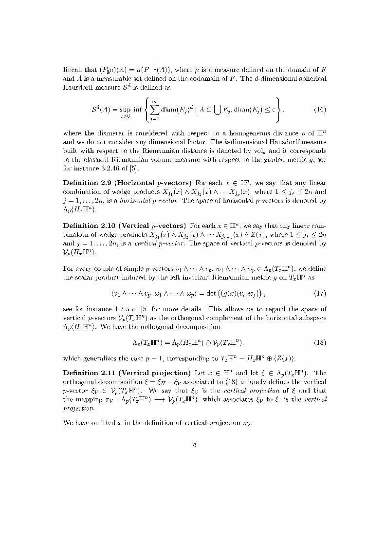
Recall that (F]�)(A) = �(F�1(A)), where � is a measure de�ned on the domain of Fand A is a measurable set de�ned on the codomain of F . The d-dimensional sphericalHausdor� measure Sd is de�ned as

Sd(A) = sup">0

inf

8<:

1Xj=1

diam(Ej)d j A �

[Ej ;diam(Ej) � "

9=; ; (16)

where the diameter is considered with respect to a homogeneous distance � of Hn

and we do not consider any dimensional factor. The k-dimensional Hausdor� measurebuilt with respect to the Riemannian distance is denoted by volk and it correspondsto the classical Riemannian volume measure with respect to the graded metric g, seefor instance 3.2.46 of [5].

De�nition 2.9 (Horizontal p-vectors) For each x 2 Hn, we say that any linear

combination of wedge products Xj1(x) ^Xj2(x) ^ � � �Xjp(x), where 1 � js � 2n andj = 1; : : : ; 2n, is a horizontal p-vector. The space of horizontal p-vectors is denoted by�p(HxH

n).

De�nition 2.10 (Vertical p-vectors) For each x 2 Hn, we say that any linear com-bination of wedge products Xj1(x) ^Xj2(x) ^ � � �Xjp�1(x) ^ Z(x), where 1 � js � 2nand j = 1; : : : ; 2n, is a vertical p-vector. The space of vertical p-vectors is denoted byVp(HxH

n).

For every couple of simple p-vectors v1 ^ � � � ^ vp, w1 ^ � � � ^wp 2 �p(TxHn), we de�ne

the scalar product induced by the left invariant Riemannian metric g on TxHn as

hv1 ^ � � � ^ vp; w1 ^ � � � ^ wpi = det�(g(x)(vi; wj)

�; (17)

see for instance 1.7.5 of [5] for more details. This allows us to regard the space ofvertical p-vectors Vp(TxH

n) as the orthogonal complement of the horizontal subspace�p(HxH

n). We have the orthogonal decomposition

�p(TxHn) = �p(HxH

n)� Vp(TxHn); (18)

which generalizes the case p = 1, corresponding to TxHn = HxH

n � hZ(x)i.

De�nition 2.11 (Vertical projection) Let x 2 Hn and let � 2 �p(TxH

n). Theorthogonal decomposition � = �H + �V associated to (18) uniquely de�nes the verticalp-vector �V 2 Vp(TxH

n). We say that �V is the vertical projection of � and thatthe mapping �V : �p(TxH

n) �! Vp(TxHn), which associates �V to �, is the vertical

projection.

We have omitted x in the de�nition of vertical projection �V .

8

De�nition 2.12 (Characteristic points and transverse points) Let � � bea C1 submanifold and let x 2 �. We say that x 2 � is a characteristic point ifTx� � HxH

n and that it is a transverse point otherwise. The characteristic set of �is the subset of all characteristic points and it is denoted by C(�).

Recall that a tangent p-vector to a p-dimensional submanifold � of class C1 at x 2 � isde�ned by the wedge product t1^t2^� � �^tp, where (t1; : : : ; tp) is an orthonormal basisof Tx�. We denote this simple p-vector by ��(x). Notice that the tangent p-vector(which belongs to a one-dimensional space) cannot be continuously de�ned on all of�, unless the submanifold is oriented.

De�nition 2.13 (Vertical tangent p-vector) Let � � be a p-dimensional sub-manifold of class C1 and let x 2 �. A vertical tangent p-vector to � at x is de�ned by�V(��), where �� is a tangent p-vector and �V is the vertical projection. The verticaltangent p-vector will be denoted by ��;V(x).

3 Blow-up at transverse points

This section is devoted to the proof of Theorem 1.1. In the following proposition, wegive a simple characterization of characteristic points using vertical tangent p-vectors.

Proposition 3.1 Let � � be a submanifold of class C1 and let x 2 �. Then

x 2 C(�) if and only if ��;V(x) = 0.

Proof. Let x 2 � and let (t1; t2; : : : ; tp) be an orthonormal basis of Tx�. We havethe unique decomposition tj = Vj + j Z; where Vj 2 HxH

n for every j = 1; : : : ; p. Itfollows that

� = t1 ^ t2 ^ � � � ^ tp

= (V1 + 1Z) ^ (V2 + 2Z) ^ � � � ^ (Vp + pZ)

= V1 ^ V2 ^ � � � ^ Vp +

pXj=1

j V1 ^ V2 ^ � � �Vj�1 ^ Z ^ Vj+1 ^ � � � ^ Vp:

Assume that x =2 C(�). If V1; V2; : : : ; Vp are linearly dependent, then we get

t1 ^ t2 ^ � � � ^ tp =

pXj=1

j V1 ^ V2 ^ � � �Vj�1 ^ Z ^ Vj+1 ^ � � � ^ Vp:

As a result, �V(�) = � hence it is not vanishing. If V1; : : : ; Vp are linearly independent,then all wedge products of the form

V1 ^ V2 ^ � � �Vj�1 ^ Z ^ Vj+1 ^ � � � ^ Vp (19)

9

are non-vanishing for every j = 1; : : : ; p. The fact that x is transverse implies thatthere exists j0 6= 0, then the projection

�V(�) =

pXj=1

j V1 ^ V2 ^ � � �Vj�1 ^ Z ^ Vj+1 ^ � � � ^ Vp (20)

is non-vanishing. Conversely, if �V(�) 6= 0, then (20) yields some j1 6= 0, thereforetj1 =2 HxH

n. 2

Proposition 3.2 Let f : �! Rk be of class C1, with surjective di�erential at each

point of . Let � denote the submanifold f�1(0) of and let x 2 �. Then x 2 C(�)if and only if df(x)jHxH

n is not surjective.

Proof. We �rst notice that Ker�df(x)jHxH

n

�= Tx� \HxH

n; then we have

dim(HxHn \ Tx�) = 2n� dim

�Im (df(x)jHxH

n)�: (21)

This last formula allows us to get our claim as follows. Assume that x 2 C(�). ThenTx� � HxH

n and (21) gives

2n+ 1� k = 2n� dim�Im (df(x)jHxH

n)�:

From this equation we conclude that df(x)jHxHn is not surjective. Conversely, if

df(x)jHxHn is not surjective, then (21) implies

dim(HxHn \ Tx�) � 2n� k + 1 = dim(Tx�)

therefore Tx� � HxHn, namely, x 2 C(�). 2

Theorem 3.3 Let f : �! Rk be of class C1, with surjective di�erential at each

point of . Let � denote the submanifold f�1(0) of and let x 2 �. Then we have

j��;V(x)j =JHf(x)

Jgf(x): (22)

Proof. Left invariance of Riemannian metric allows us to consider the left translatedsubmanifold lx�1�. Replacing f with f � lx and with lx�1 we can assume that x isthe unit element 0 of Hn. Recall that lx : H

n �! Hn is the left translation lx(y) = x�y.

If x 2 C(�), then Proposition 3.1 and Proposition 3.2 make (22) the trivial identity0 = 0. Assume that x 2 � n C(�). Then Proposition 3.2 implies that the horizotalgradients

rHfi = (X1f

i(0); X2fi(0); : : : ; X2nf

i(0)) for i = 1; 2; : : : ; k

10

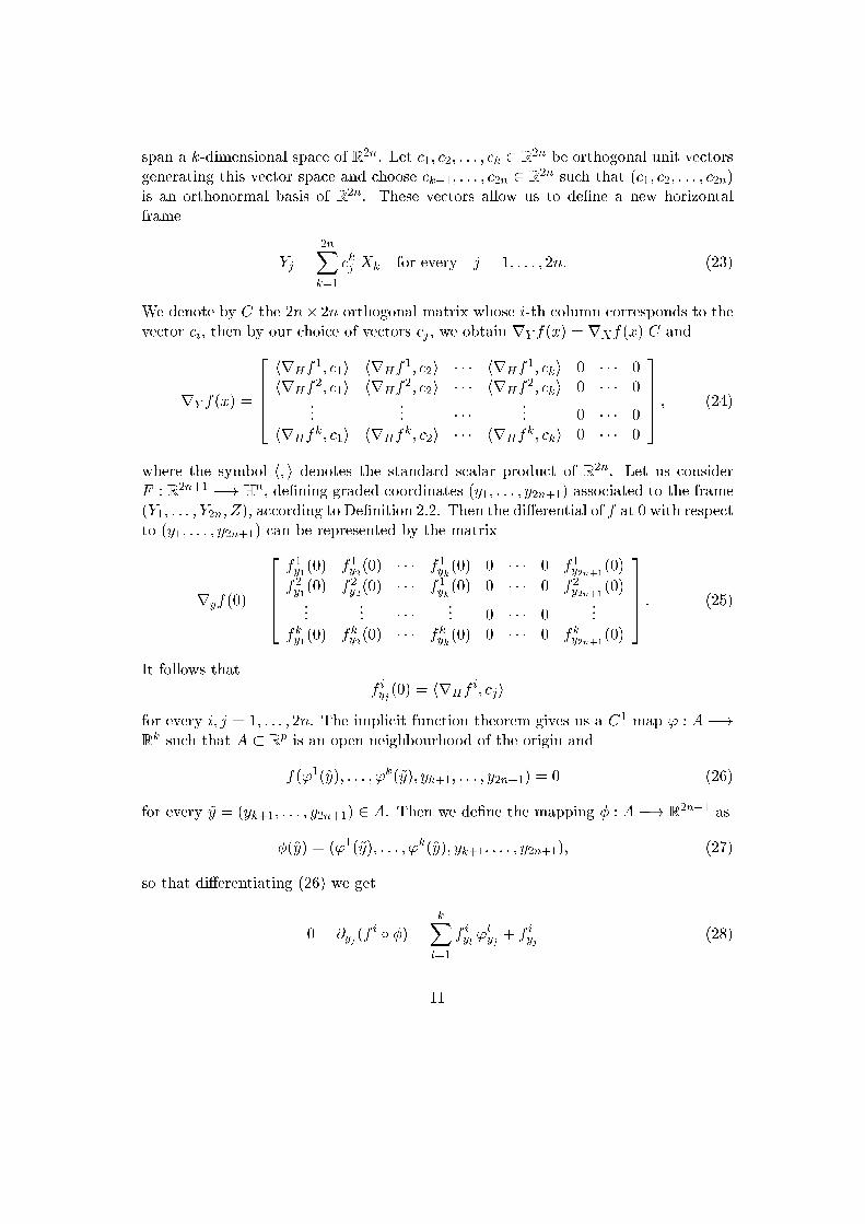
span a k-dimensional space of R2n. Let c1; c2; : : : ; ck 2 R2n be orthogonal unit vectors

generating this vector space and choose ck+1; : : : ; c2n 2 R2n such that (c1; c2; : : : ; c2n)

is an orthonormal basis of R2n. These vectors allow us to de�ne a new horizontalframe

Yj =2nXk=1

ckj Xk for every j = 1; : : : ; 2n: (23)

We denote by C the 2n� 2n orthogonal matrix whose i-th column corresponds to thevector ci, then by our choice of vectors cj , we obtain rY f(x) = rXf(x) C and

rY f(x) =

26664hrHf

1; c1i hrHf1; c2i � � � hrHf

1; cki 0 � � � 0hrHf

2; c1i hrHf2; c2i � � � hrHf

2; cki 0 � � � 0...

... � � �... 0 � � � 0

hrHfk; c1i hrHf

k; c2i � � � hrHfk; cki 0 � � � 0

37775 ; (24)

where the symbol h; i denotes the standard scalar product of R2n. Let us considerF : R2n+1 �! H

n, de�ning graded coordinates (y1; : : : ; y2n+1) associated to the frame(Y1; : : : ; Y2n; Z), according to De�nition 2.2. Then the di�erential of f at 0 with respectto (y1; : : : ; y2n+1) can be represented by the matrix

ryf(0) =

26664f1y1(0) f1y2(0) � � � f1yk(0) 0 � � � 0 f1y2n+1(0)

f2y1(0) f2y2(0) � � � f1yk(0) 0 � � � 0 f2y2n+1(0)...

... � � �... 0 � � � 0

...fky1(0) fky2(0) � � � fkyk(0) 0 � � � 0 fky2n+1(0)

37775 : (25)

It follows thatf iyj (0) = hrHf

i; cji

for every i; j = 1; : : : ; 2n. The implicit function theorem gives us a C1 map ' : A �!Rk such that A � Rp is an open neighbourhood of the origin and

f('1(~y); : : : ; 'k(~y); yk+1; : : : ; y2n+1) = 0 (26)

for every ~y = (yk+1; : : : ; y2n+1) 2 A. Then we de�ne the mapping � : A �! R2n+1 as

�(~y) = ('1(~y); : : : ; 'k(~y); yk+1; : : : ; y2n+1); (27)

so that di�erentiating (26) we get

0 = @yj (fi � �) =

kXl=1

f iyl 'lyj + f iyj (28)

11

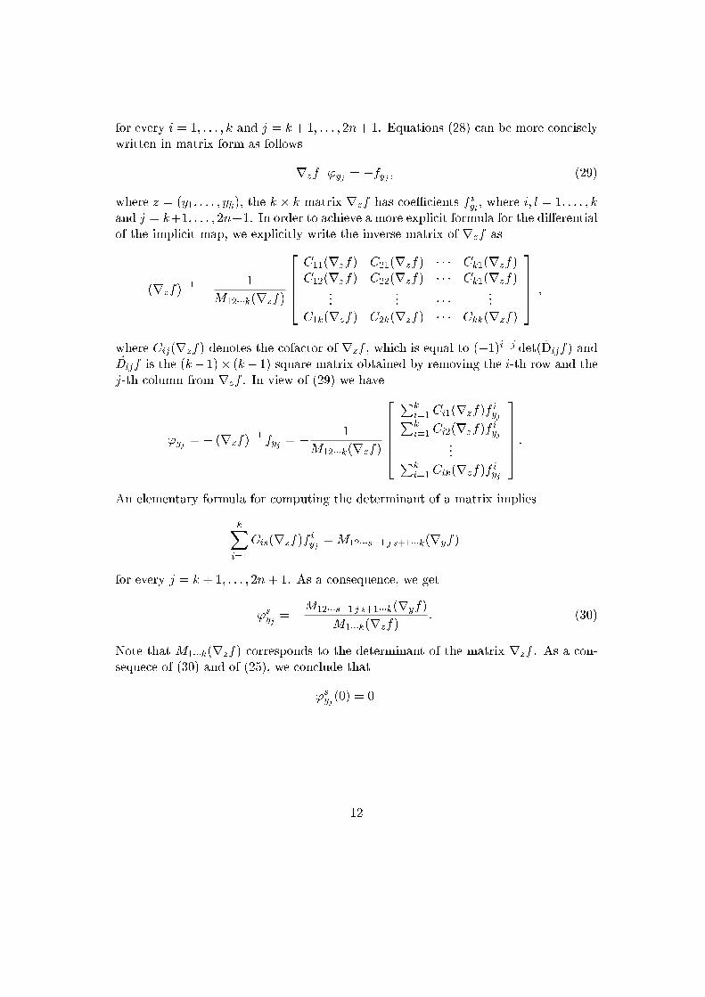
for every i = 1; : : : ; k and j = k+1; : : : ; 2n+1. Equations (28) can be more conciselywritten in matrix form as follows

rzf 'yj = �fyj ; (29)

where z = (y1; : : : ; yk), the k � k matrix rzf has coe�cients f iyl , where i; l = 1; : : : ; kand j = k+1; : : : ; 2n+1. In order to achieve a more explicit formula for the di�erentialof the implicit map, we explicitly write the inverse matrix of rzf as

(rzf)�1 =

1

M12���k(rzf)

26664C11(rzf) C21(rzf) � � � Ck1(rzf)C12(rzf) C22(rzf) � � � Ck1(rzf)

...... � � �

...C1k(rzf) C2k(rzf) � � � Ckk(rzf)

37775 ;

where Cij(rzf) denotes the cofactor of rzf , which is equal to (�1)i+j det(Dijf) andDijf is the (k� 1)� (k� 1) square matrix obtained by removing the i-th row and thej-th column from rzf . In view of (29) we have

'yj = � (rzf)�1 fyj = �

1

M12���k(rzf)

266664

Pki=1Ci1(rzf)f

iyjPk

i=1Ci2(rzf)fiyj

...Pki=1Cik(rzf)f

iyj

377775 :

An elementary formula for computing the determinant of a matrix implies

kXi=1

Cis(rzf)fiyj =M12���s�1 j s+1���k(ryf)

for every j = k + 1; : : : ; 2n+ 1. As a consequence, we get

'syj = �M12���s�1 j s+1���k(ryf)

M1���k(rzf): (30)

Note that M1���k(rzf) corresponds to the determinant of the matrix rzf . As a con-sequece of (30) and of (25), we conclude that

'syj (0) = 0

12

for every j = k+1; : : : ; 2n. Previous considerations and expression (27) lead us to theformula

r~y�(0) =

26666666666666664

0 0 � � � 0 '1y2n+1(0)

0 0 � � � 0 '2y2n+1(0)...

.... . .

......

0 0 � � � 0 'ky2n+1(0)

1 0 � � � 0 00 1 � � � 0 0... 0

. . . 0 0...

.... . . 1

...0 0 � � � 0 1

37777777777777775

; (31)

where r~y�(0) is a (2n+ 1)� p matrix whose p� p lower block is the identity matrix.Notice that columns of (31) represent a basis of the tangent space T0� with respectto coordinates (yk+1; : : : ; y2n+1). More precisely, the set of vectors0

B@Yk+1(0); Yk+2(0); : : : ; Y2n(0); Z(0) +Pk

j=1 vj Yj(0)�1 +

Pkj=1 v2j

�1=21CA

form an orthonormal basis of T0�, where we have de�ned vj = 'jy2n+1(0). Then thetangent p-vector �� to � at 0 is given by the wedge product

��(0) =Yk+1(0) ^ Yk+2(0) ^ � � � ^ Y2n(0) ^

�Z(0) +

Pkj=1 vj Yj(0)

��1 +

Pkj=1 v2j

�1=2 :

Obviously, p-vectors Yk+1(0)^Yk+2(0)^ � � � ^Y2n(0)^Yj(0) are horizontal, hence theydisappear in the vertical projection. It follows that

��;V(0) = �V(��;V(0)) =Yk+1(0) ^ Yk+2(0) ^ � � � ^ Y2n(0) ^ Z(0)�

1 +Pk

j=1 v2j

�1=2 ;

therefore we clearly obtain

j��;V(0)j =�1 +

kXl=1

v2l

��1=2: (32)

Due to formula (30) in the case j = 2n+ 1 and to (25), we obtain

1 +kXl=1

v2l =(M1���k(rzf))

2+Pk

s=1 (M12���s�1 2n+1 s+1���k(ryf))2

(M1���k(rzf))2 =

�Jgf(0)

JHf(0)

�2;

13

then (32) shows the valdity of (22) in the case x = 0. Left invariance of the Riemannianmetric g leads us to the conclusion. 2

De�nition 3.4 (Metric factor) Let � be a vertical simple p-vector of �p(hn) and

let L(�) be the unique associated subspace, with L = expL(�). The metric factor ofa homogeneous distance � with respect to � is de�ned by

��p(�) = Hpj�j

�F�1(L \B1)

�;

where F : R2n+1 �! Hn de�nes a system of graded coordinates, Hp

j�j denotes the

p-dimensional Hausdor� measure with respect to the Euclidean distance of R2n+1 andB1 is the unit ball of Hn with respect to the distance �. Recall that the subspaceassociated to a simple p-vector � is de�ned as fv 2 hn j v ^ � = 0g.

Remark 3.5 In the case of subspaces L of codimension one, the notion of metricfactor �ts into the one introduced in [19]. It is easy to observe that the notion ofmetric factor does not depend on the system of coordinates we are using. In fact,F�11 � F2 : R2n+1 �! R

2n+1 is an Euclidean isometry whenever F1; F2 : R2n+1 �!Hn represent systems of graded coordinates with respect to the same left invariant

Riemannian metric.

Proof of Theorem 1.1. As in the proof of Theorem 3.3, left invariance of the Rieman-nian metric g allows us to assume that x = 0. For r0 > 0 su�ciently small, we cansuppose the existence of a function f : Br0 �! R

k such that � \ Br0 = f�1(0) andwhose di�erential is surjective at every point of Br0 . By Proposition 3.2, the horizontalgradients

rHfi = (X1f

i(0); X2fi(0); : : : ; X2nf

i(0)) for i = 1; 2; : : : ; k

span a k-dimensional space of R2n. Now, repeating the argument in the proof ofTheorem 3.3, we de�ne the system of graded coordinates (y1; : : : ; y2n+1) associated tothe frame (Y1; : : : ; Y2n; Z), where Yj are given by (23). The di�erential of f at 0 canbe represented by the matrix

ryf(0) =

26664f1y1(0) f1y2(0) � � � f1yk(0) 0 � � � 0 f1y2n+1(0)

f2y1(0) f2y2(0) � � � f1yk(0) 0 � � � 0 f2y2n+1(0)...

... � � �... 0 � � � 0

...fky1(0) fky2(0) � � � fkyk(0) 0 � � � 0 fky2n+1(0)

37775 ; (33)

whose �rst k columns are linearly independent. By the implicit function theorem thereexists a C1 mapping ' : A �! R

k such that A � Rp is an open neighbourhood of theorigin and

f('1(~y); : : : ; 'k(~y); yk+1; : : : ; y2n+1) = 0 (34)

14

for every ~y = (yk+1; : : : ; y2n+1) 2 A. Proceeding as in the proof of Theorem 3.3, wede�ne the mapping � : A �! R

2n+1 as

�(~y) = ('1(~y); : : : ; 'k(~y); yk+1; : : : ; y2n+1); (35)

and by the same computations, di�erentiating (34) we obtain

r~y�(0) =

26666666666666664

0 0 � � � 0 '1y2n+1(0)

0 0 � � � 0 '2y2n+1(0)...

.... . .

......

0 0 � � � 0 'ky2n+1(0)

1 0 � � � 0 00 1 � � � 0 0... 0

. . . 0 0...

.... . . 1

...0 0 � � � 0 1

37777777777777775

; (36)

wherer~y�(0) is a (2n+1)�pmatrix whose p�p lower block is the identity matrix. Foreach r < r0, write the ball Br in terms of graded coordinates de�ning ~Br = F�1(Br) �R2n+1. The surface � read in graded coordinates can be seen as the image of �. Then

we have established

volp(� \Br)

rp+1= r�1�p

Z��1( ~Br)

Jg�(~y) d~y : (37)

The dilation �r restricted to coordinates (y1; : : : ; y2n+1) gives

�r~y = �r((yk+1; : : : ; y2n+1)) = (ryk+1; ryk+2; : : : ; ry2n; r2y2n+1); (38)

therefore, performing a change of variable in (37) we get

volp(� \Bx;r)

rp+1=

Z�1=r(��1( ~Br))

Jg�(�r~y) d~y : (39)

The set �1=r(��1( ~Br)) can be written as follows

(�1=r � � � �r)�1( ~B1) =

�~y 2 Rp

�����'1(�r~y)

r; : : : ;

'k(�r~y)

r; yk+1; : : : ; y2n+1

�2 ~B1

�:(40)

From expressions (36) and (38) one easily gets that

limr!0+

'j(�r~y)

r= 0 (41)

15

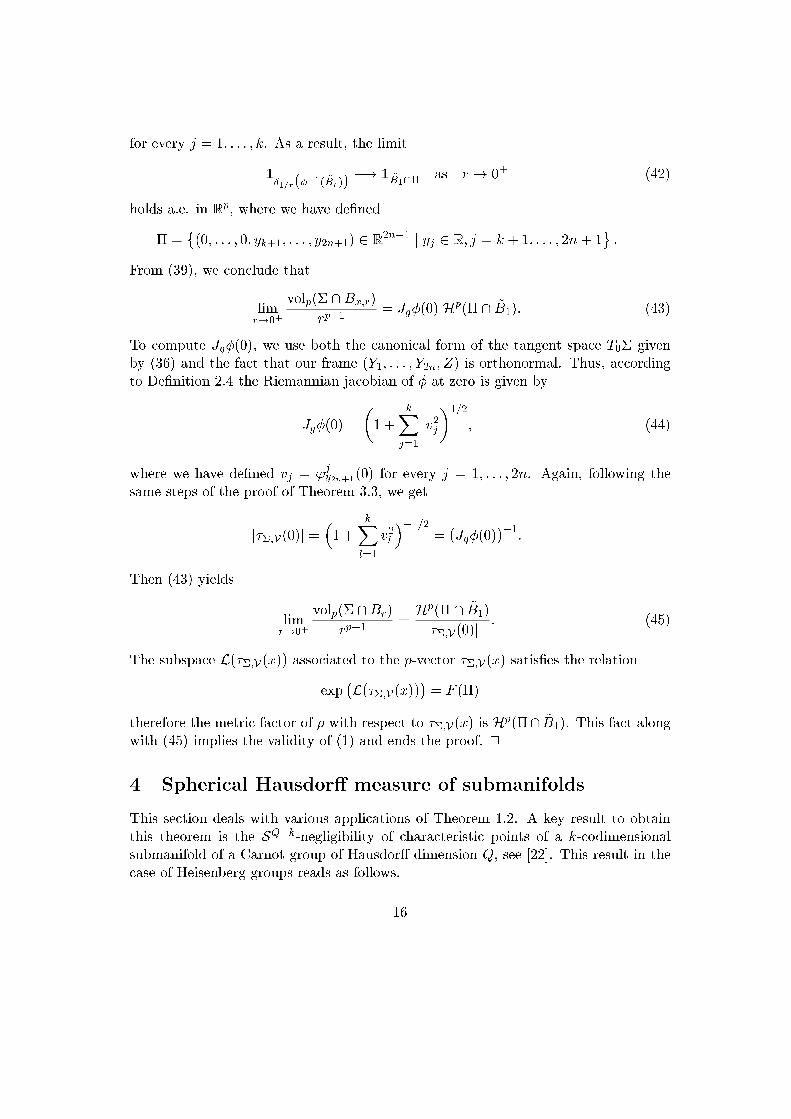
for every j = 1; : : : ; k. As a result, the limit

1�1=r(��1( ~Br))

�! 1 ~B1\�as r ! 0+ (42)

holds a.e. in Rp, where we have de�ned

� =�(0; : : : ; 0; yk+1; : : : ; y2n+1) 2 R

2n+1 j yj 2 R; j = k + 1; : : : ; 2n+ 1:

From (39), we conclude that

limr!0+

volp(� \Bx;r)

rp+1= Jg�(0) H

p(� \ ~B1): (43)

To compute Jg�(0), we use both the canonical form of the tangent space T0� givenby (36) and the fact that our frame (Y1; : : : ; Y2n; Z) is orthonormal. Thus, accordingto De�nition 2.4 the Riemannian jacobian of � at zero is given by

Jg�(0) =

�1 +

kXj=1

v2j

�1=2; (44)

where we have de�ned vj = 'jy2n+1(0) for every j = 1; : : : ; 2n. Again, following thesame steps of the proof of Theorem 3.3, we get

j��;V(0)j =�1 +

kXl=1

v2l

��1=2= (Jg�(0))

�1:

Then (43) yields

limr!0+

volp(� \Br)

rp+1=Hp(� \ ~B1)

j��;V(0)j: (45)

The subspace L(��;V(x)) associated to the p-vector ��;V(x) satis�es the relation

exp�L(��;V(x))

�= F (�)

therefore the metric factor of � with respect to ��;V(x) is Hp(�\ ~B1). This fact along

with (45) implies the validity of (1) and ends the proof. 2

4 Spherical Hausdor� measure of submanifolds

This section deals with various applications of Theorem 1.2. A key result to obtainthis theorem is the SQ�k-negligibility of characteristic points of a k-codimensionalsubmanifold of a Carnot group of Hausdor� dimension Q, see [22]. This result in thecase of Heisenberg groups reads as follows.

16

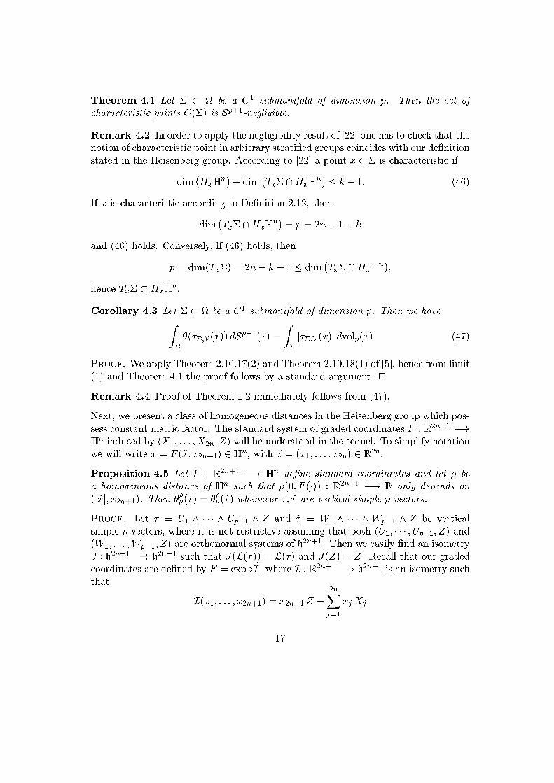
Theorem 4.1 Let � � be a C1 submanifold of dimension p. Then the set of

characteristic points C(�) is Sp+1-negligible.

Remark 4.2 In order to apply the negligibility result of [22] one has to check that thenotion of characteristic point in arbitrary strati�ed groups coincides with our de�nitionstated in the Heisenberg group. According to [22] a point x 2 � is characteristic if

dim (HxHn)� dim (Tx� \HxH

n) � k � 1: (46)

If x is characteristic according to De�nition 2.12, then

dim (Tx� \HxHn) = p = 2n+ 1� k

and (46) holds. Conversely, if (46) holds, then

p = dim(Tx�) = 2n� k + 1 � dim (Tx� \HxHn);

hence Tx� � HxHn.

Corollary 4.3 Let � � be a C1 submanifold of dimension p. Then we haveZ��(��;V(x)) dS

p+1(x) =

Z�j��;V(x)j dvolp(x) (47)

Proof. We apply Theorem 2.10.17(2) and Theorem 2.10.18(1) of [5], hence from limit(1) and Theorem 4.1 the proof follows by a standard argument. 2

Remark 4.4 Proof of Theorem 1.2 immediately follows from (47).

Next, we present a class of homogeneous distances in the Heisenberg group which pos-sess constant metric factor. The standard system of graded coordinates F : R2n+1 �!Hn induced by (X1; : : : ; X2n; Z) will be understood in the sequel. To simplify notation

we will write x = F (~x; x2n+1) 2 Hn, with ~x = (x1; : : : ; x2n) 2 R

2n.

Proposition 4.5 Let F : R2n+1 �! Hn de�ne standard coordintates and let � be

a homogeneous distance of Hn such that �(0; F (�)) : R2n+1 �! R only depends on

(j~xj; x2n+1). Then ��p(�) = ��p(~�) whenever �; ~� are vertical simple p-vectors.

Proof. Let � = U1 ^ � � � ^ Up�1 ^ Z and ~� = W1 ^ � � � ^ Wp�1 ^ Z be verticalsimple p-vectors, where it is not restrictive assuming that both (U1; � � � ; Up�1; Z) and(W1; : : : ;Wp�1; Z) are orthonormal systems of h

2n+1. Then we easily �nd an isometryJ : h2n+1 �! h2n+1 such that J(L(�)) = L(~�) and J(Z) = Z. Recall that our gradedcoordinates are de�ned by F = exp �I, where I : R2n+1 �! h2n+1 is an isometry suchthat

I(x1; : : : ; x2n+1) = x2n+1 Z +2nXj=1

xj Xj

17

for every (x1; : : : ; x2n+1) 2 R2n+1. Thus, de�ning ~B1 = F�1(B1) � R

2n+1, we have

F�1( expL(~�) \B1) = I�1 � J(L(�)) \ ~B1 = '(I�1(L(�))) \ ~B1 ; (48)

where ' = I�1�J�I : R2n+1 �! R2n+1 is an Euclidean isometry such that '(e2n+1) =

e2n+1 and e2n+1 is the (2n+1)-th vector of the canonical basis of R2n+1. Then j~xj = j~yj

whenever '(~x; t) = (~y; t). As a result, the fact that �(0; F (~x; t)) only depends on (j~xj; t)easily implies that '( ~B1) = ~B1. Thus, due to (48), it follows that

��p(�) = Hpj�j(I

�1(L(�)) \ ~B1) = Hpj�j('(I

�1(L(�))) \ ~B1) = ��p(~�): (49)

This ends the proof. 2

Example 4.6 An example of homogeneous distance satisfying hypotheses of Propo-sition 4.5 is the gauge distance, also called Kor�anyi distance, [15]. The gauge distancefrom x to the origin is given by

d(x; 0) = (j~xj4 + 16x22n+1)1=4

;

where x = (~x; x2n+1). Then we de�ne d(x; y) = d(0; x�1y), for any x; y 2 Hn. Ano-ther example of homogeneous distance with this property is the \maximum distance",de�ned by

d1(x; 0) = maxnj~xj; jx2n+1j

1=2o:

Due to Proposition 4.5, both of these distances have constant metric factor.

Next, we apply (2) to compute the spherical Hausdor� measure of some submanifolds.We will use the following proposition.

Proposition 4.7 Let � : U �! R2n+1 be a C1 embedding, where U � Rp is a bounded

open set. Let F : R2n+1 �! Hn de�ne standard coordinates and set � = F �� : U �!

Hn, where � = �(U). Let � be a homogeneous distance with constant metric factor

� > 0. Then we have

Sp+1Hn

(�) =

ZU

���V(�u1(u) ^ �u2(u) ^ � � � ^ �up(u))�� du ; (50)

for every measurable set A � Hn, where the norm j � j is induced by the scalar product

(17) on p-vectors.

Proof. By de�nition of Riemannian volume, formula (2) can be written with respectto � as

Sp+1Hn

(�) =

ZUj��;V(�(u))j

qdet�g(�(u))(�ui(u);�uj (u))

�du ; (51)

18

where we have

���u1(u) ^ �u2(u) ^ � � � ^ �up(u)�� =qdet

�g(�(u))(�ui(u);�uj (u))

�: (52)

Therefore, taking into account the formula

��(�(u)) =�u1(u) ^ �u2(u) ^ � � � ^ �up(u)

j�u1(u) ^ �u2(u) ^ � � � ^ �up(u)j; (53)

the de�nition of vertical tangent p-vector �V(��) = ��;V and joining (51), (52) and(53), formula (50) follows. 2

Example 4.8 Let � : R3 �! R5, de�ned by �(u) = (u1; u2; u3; 0;

u21+u2

2+u2

3

2 ). Themapping � parametrizes a 3-dimensional paraboloid � = �(U) of R5, where U is anopen bounded set of R3, � = F �� and F : R3 �! H

2 represents standard coordinates,according to De�nition 2.2. Using expressions (7), we have

�u1(u) =~X1(�(u)) + (�3(u) + u1) ~T (�(u)) ;

�u2(u) =~X2(�(u)) + (�4(u) + u2) ~T (�(u)) ;

�u3(u) =~X3(�(u)) + (u3 � �1(u)) ~T (�(u)) :

Observing that for every j = 1; : : : ; 2n, we have

dF (�(u)) ~Xj(�(u)) = Xj(�(u)) 2 H�(u)Hn and

dF (�(u)) ~Z(�(u)) = Z(�(u)) 2 T�(u)Hn ;

hence we obtain

�u1(u) = X1(�(u)) + (u3 + u1)T (�(u)) ; �u2(u) = X2(�(u)) + u2T (�(u)) ;

�u3(u) = X3(�(u)) + (u3 � u1)T (�(u)) :

Thus, we can compute

�V(�u1 ^ �u2 ^ �u3)

= (u3 � u1)X1 ^X2 ^ T � u2X1 ^X3 ^ T + (u3 + u1)X2 ^X3 ^ T ;

hence formula (50) yields

S4H2(�) =

ZU

qu22 + 2(u23 + u21) du :

19

Example 4.9 Let � : R2 �! R3, �(u1; u2) = (a1u1; a2u2; bu1 + cu2), de�ne a hyper-

plane in R3, where a1; a2; b; c 2 R and (J�)2 = a21a22 + a21c

2 + a22b2 > 0. Embedding

the hyperplane in H1 through standard coordinates F : R3 �! H1, we obtain

�u1(u) = a1X1(�(u)) + (a1a2u2 + b)T (�(u)) ;

�u2(u) = a2X2(�(u)) + (c� a1a2u1)T (�(u)) ;

where � = F � �. Then we get

�V(�u1(u) ^ �u2(u)) = a1(c� a1a2u1)X1 ^ T � (a1a2u2 + b)a2X2 ^ T

and formula (50) yields

S3H1(�) =

ZU

qa21(c� a1a2u1)2 + a22(a1a2u2 + b)2 du; (54)

where � = �(U) and U is an open bounded set of R2.

Example 4.10 Let � : R2 �! R3, �(u1; u2) = (u1; u2;

u21+u2

2

2 ), de�ne a paraboloid inR3. By standard coordinates F : R3 �! H

1 and arguing as in the previous examples,we have

�u1(u) = X1(�(u)) + (u2 + u1)T (�(u)) and

�u2(u) = X2(�(u)) + (u2 � u1)T (�(u)) ;

where � = F � �. It follows that

�V(�u1(u) ^ �u2(u)) = (u2 � u1)X1 ^ T � (u2 + u1)X2 ^ T

and formula (50) yields

S3H1(P) =

ZU

q2u21 + 2u22 du (55)

where P = �(U) and U is an open bounded set of R2.

Remark 4.11 It is curious to notice that the density of S3H1

restricted to the paraboloidP, computed in (55), is proportional to the density of S3

H1restricted to the horizontal

projection of P onto the plane F (f(x1; x2; x3) j x3 = 0g) � H1, whose density is givenby (54) in the case a1 = a2 = 1 and b = c = 0.

Example 4.12 From computations of Example 4.9, one can get the 2-dimensionalspherical Hausdor� measure of the line �(t) = F (at; 0; bt) de�ned on an interval [�; �].We have

�0(t) = aX1(�(t)) + bT (�(t)) and �V(�0(t)) = bT (�(t)) ; (56)

then de�ning the submanifold L = �([�; �]), the formula S2H1(L) = jbj (� � �) holds.

20

Another consequence of (2) is the lower semicontinuity of the spherical Hausdor�measure with respect to weak convergence of regular currents. To see this, it su�cesto establish the following formula

Sp+1Hn

(�) = sup!2Fp

c ()

Z�h��;V ; !i dvolp ; (57)

where Fpc () is the space of smooth p-forms with compact support in with j!j � 1.

The norm of ! is de�ned making the standard frame of p-forms (dx1; dx2; : : : ; dx2n; ~�)orthonormal and extending this scalar product to p-forms exactly as we have seen informula (17). The 1-form ~� is the so called contact form

~� = dx2n+1 +nX

j=1

xj+n dxj � xj dxj+n (58)

written in standard coordinates. Note that (dx1; dx2; : : : ; dx2n; ~�) is the dual basis of( ~X1; : : : ; ~X2n; ~Z). Formula (57) follows from (2) observing thatZ

�j��;V j dvolp = sup

!2Fpc ()

Z�h��;V ; !i dvolp ; (59)

as one can check by standard arguments. As a consequence of these observations, wecan establish the following proposition.

Proposition 4.13 Let (�m) be a sequence of C1 submanifolds of which weakly

converges in the sense of currents to the C1 submanifold �. Then

lim infm�!1

Sp+1Hn

(�m) � Sp+1Hn

(�): (60)

Proof. By hypothesisZ�m

h��m;V ; !i dvolp �!

Z�h��;V ; !i dvolp ; (61)

for every ! 2 Fpc (). Then (57) ends the proof. 2

Remark 4.14 It is clear the importance of (60) in studying versions of the Plateauproblem with respect to the geometry of Heisenberg groups.

Recall that the horizontal normal is the orthogonal projection of the normal to �(x)to Tx� onto the horizontal subspace HxH

n. In the next proposition we show that incodimension one an explicit relationship can be established between vertical tangent2n-vector and horizontal normal �H .

21

Proposition 4.15 Let � be a 2n-dimensional submanifold of class C1 and let �H(x)a horizontal normal at x 2 �. Then we have

�jH = (�1)j � j�;V

where �H =P2n

j=1 �jH Xj and ��;V =

P2nj=1 �

j�;V X1 ^ � � �Xj�1 ^Xj+1 ^ � � �X2n ^Z: In

particular, the equality j��;V j = j�H j holds.

Proof Let (t1; t2; : : : ; t2n) be an orthonormal basis of Tx�, where x is a transversepoint. Then

tj =2nXi=1

cij Xi(x) + c2n+1j Z(x)

where C = (cij) is a (2n+ 1)� 2n matrix, whose columns are orthonormal vectors of

R2n+1. Then we have

��(x) = t1 ^ t2 ^ � � � ^ t2n =2n+1Xj=1

det(Cj) X1 ^X2 ^ � � � ^Xj�1 ^Xj+1 ^ � � � ^ Z ;

where Cjis the 2n � 2n matrix obtained by removing the j-th row from C. The

vertical projection yields

��;V(x) = �V(��(x)) =2nXj=1

det(Cj) X1 ^X2 ^ � � � ^Xj�1 ^Xj+1 ^ � � � ^ Z (62)

and by elementary linear algebra one can deduce that

2n+1Xj=1

(�1)j det(Cj) cjk = det

�C ck

�= 0 (63)

for every k = 1; : : : ; 2n. Then the vector

� =2nXj=1

(�1)j det(Cj) Xj + (�1)2n+1 det(C

2n+1) Z

yields a unit normal to � at x. Its horizontal projection is

�H =2nXj=1

(�1)j det(Cj) Xj : (64)

Formulae (62) and (64) yield the thesis. 2

22

5 Coarea formula

This section is devoted to the proof of Theorem 1.3. Next, we recall the Riemanniancoarea formula, see Section 13.4 of [4].

Theorem 5.1 Let f : Hn �! Rk be a Riemannian Lipschitz function, with 1 � k <

2n+ 1. Then for any summable map u : Hn �! R, the following formula holdsZHn

u(x) Jgf(x) dvol2n+1(x) =

ZRk

�Zf�1(t)

u(y) dvolp(y)

�dt ; (65)

where p = 2n+ 1� k

In the previous theorem the Heisenberg group Hn is equipped with its left invariantRiemannian metric g. The terminology \Riemannian Lipschitz map" means that themap is Lipschitz with respect to the Riemannian distance.

Proof of Theorem 1.3. We �rst prove (4) in the case f is de�ned on all of Hn and isof class C1. Let be an open subset of Hn. In view of Riemannian coarea formula(65), we have

Zu(x)Jgf(x) dx =

ZRk

Zf�1(t)\

u(y) dvolp(y)

!dt; (66)

where u : �! [0;+1] is a measurable function. Note that in the left hand side of(66) we have used the Lebesgue measure in that, by Proposition 2.7, it coincides withthe volume measure expressed in terms of standard coordinates, namely F](L

2n+1) =vol2n+1. Now we de�ne

u(x) = JHf(x)1fJf 6=0g\(x)=Jf(x)

and use (66), obtaining

ZJHf(x) dx =

ZRk

Zf�1(t)\

JHf(x)1fJf 6=0g(x)

Jf(x)dvolp(y)

!dt: (67)

The validity of (66) also implies that for a.e. t 2 Rk the set of points of f�1(t) whereJgf vanishes is volp-negligible, then the previous formula becomes

ZJHf(x) dx =

ZRk

Zf�1(t)\

JHf(x)

Jf(x)dvolp(y)

!dt: (68)

By classical Sard's theorem and Theorem 4.1 for a.e. t 2 Rk the C1 submanifold

f�1(t) has Sp+1Hn

-negligible characteristic points, hence Proposition 3.2 implies that

Ct = fy 2 f�1(t) \ j JHf(y) = 0g

23

is Sp+1Hn

-negligible. As a result, from formulae (22) and (2) we have proved that fora.e. t 2 Rk the equalitiesZ

f�1(t)\

JHf(x)

Jgf(x)dvolp(y) = Sp+1

Hn(f�1(t) \ n Ct) = Sp+1

Hn(f�1(t) \ )

hold, therefore (68) yieldsZJHf(x) dx =

ZRk

Sp+1Hn

(f�1(t) \ ) dt: (69)

The arbitrary choice of yields the validity of (69) also for arbitrary closed sets.Then, approximation of measurable sets by closed ones, Borel regularity of Sp+1

Hnand

the coarea estimate 2.10.25 of [5] extend the validity of (69) to the following oneZAJHf(x) dx =

ZRk

Sp+1Hn

(f�1(t) \A)dt; (70)

where A is a measurable subset of Hn. Now we consider the general case, wheref : A �! R

k is a Lipschitz map de�ned on a measurable bounded subset A of H3.Let f1 : Hn �! R

k be a Lipschitz extension of f , namely, f1jA = f holds. Due tothe Whitney extension theorem (see for instance 3.1.15 of [5]) for every arbitrarily�xed " > 0 there exists a C1 function f2 : Hn �! R

k such that the open subsetO = fz 2 Hn j f1(z) 6= f2(z)g has Lebesgue measure less than or equal to ". We wishto prove ����

ZAJHf(x) dx�

ZRk

Sp+1Hn

(f�1(t) \A)dt

���� �ZA\O

JHf(x) dx

+

ZRk

Sp+1Hn

(f�1(t) \A \O)dt : (71)

In fact, due to the validity of (70) for C1 mappings, we haveZAnO

JHf2(x) dx =

ZRk

Sp+1Hn

(f�12 (t) \A nO) dt:

Note here that the horizontal jacobian JHf is well de�ned on A, in that df is well de-�ned at density points of the domain, see for instance De�nition 7 and Proposition 2.2of [17]. The equality f2jAnO = fjAnO implies that JHf2 = JHf a.e. on A nO, thereforeZ

AnOJHf(x) dx =

ZRk

Sp+1Hn

(f�1(t) \A nO) dt

holds and inequality (71) is proved. Now we observe that for a.e. x 2 A, we have

JHf(x) �kYi=1

� 2nXj=1

(Xjfi(x))

2�1=2

� kdf(x)jHxHnkk

24

therefore the estimate

JHf(x) � Lip(f)k (72)

holds for a.e. x 2 A. By virtue of the general coarea inequality 2.10.25 of [5] thereexists a dimensional constant c1 > 0 such thatZ

Rk

Sp+1Hn

(f�1(t) \A \O)dt � c1 Lip(f)k H2n+2(O): (73)

The fact that the 2n + 2-dimensional Hausdor� measure H2n+2 with respect to thehomogeneous distance � is proportional to the Lebesgue measure, gives us a constantc2 > 0 such thatZ

Rk

Sp+1Hn

(f�1(t) \A \O)dt � c2 Lip(f)k L2n+1(O) � c2 Lip(f)

k ": (74)

Thus, estimates (72) and (74) joined with inequality (71) yield����ZAJHf(x) dx�

ZRk

Sp+1Hn

(f�1(t) \A)dt

���� � (1 + c2) Lip(f)k ":

Letting "! 0+, we have proved thatZAJHf(x) dx =

ZRk

Sp+1Hn

(f�1(t) \A)dt: (75)

Finally, utilizing increasing sequences of step functions pointwise converging to u andapplying Beppo Levi convergence theorem the proof of (4) is achieved in the case A isbounded. If A is not bounded, then one can take the limit of (4) where A is replacedby Ak and fAkg is an increasing sequence of measurable bounded sets whose unionyields A. Then the Beppo Levi convergence theorem concludes the proof. 2

Remark 5.2 Notice that once f : A �! Rk in the previous theorem is considered

with respect to standard coordinates it is easy to check that the locally Lipschitzproperty with respect to the Euclidean distance of R2n+1 is equivalent to the locallyLipschitz property with respect to the Riemannian distance.

References

[1] L.Ambrosio, Some �ne properties of sets of �nite perimeter in Ahlfors regular

metric measure spaces, Adv. Math., 159, 51-67, (2001)

[2] Z.M.Balogh, Size of characteristic sets and functions with prescribed gradients,J. Reine Angew. Math., 564, 63-83, (2003)

25

[3] A.Bella��che, J.J.Risler eds, Sub-Riemannian geometry, Progress in Mathe-matics, 144, Birkh�auser Verlag, Basel, (1996).

[4] Y.D.Burago, V.A.Zalgaller, Geometric inequalities, Grundlehren Math.Springer, Berlin.

[5] H.Federer, Geometric Measure Theory, Springer, (1969).

[6] G.B. Folland, E.M. Stein, Hardy Spaces on Homogeneous groups, PrincetonUniversity Press, 1982

[7] B.Franchi, R.Serapioni, F.Serra Cassano, Meyers-Serrin type theorems

and relaxation of variational integrals depending on vector �elds, Houston Jour.Math., 22, 859-889, (1996)

[8] B.Franchi, R.Serapioni, F.Serra Cassano, Recti�ability and Perimeter in

the Heisenberg group, Math. Ann. 321, n. 3, (2001).

[9] B.Franchi, R.Serapioni, F.Serra Cassano, Regular hypersurfaces, intrinsicperimeter and implicit function theorem in Carnot groups, Comm. Anal. Geom.11, n.5, 909-944, (2003)

[10] B.Franchi, R.Serapioni, F.Serra Cassano, Regular submanifolds, graphs

and area formula in Heisenberg groups, preprint (2004)

[11] M.Gromov, Carnot-Carath�eodory spaces seen from within, SubriemannianGeometry, Progress in Mathematics, 144. ed. by A.Bellaiche and J.Risler,Birkhauser Verlag, Basel, (1996).

[12] N.Garofalo, D.M.Nhieu, Isoperimetric and Sobolev Inequalities for Carnot-

Carath�eodory Spaces and the Existence of Minimal Surfaces, Comm. Pure Appl.Math. 49, 1081-1144 (1996)

[13] P.Hajlasz, P.Koskela, Sobolev met Poincar�e, Mem. Amer. Math. Soc. 145,(2000)

[14] B.Kirchheim, F.Serra Cassano, Recti�ability and parametrization of intrinsic

regular surfaces in the Heisenberg group, Ann. Sc. Norm. Super. Pisa Cl. Sci. (5),3, n.4, 871-896, (2004)

[15] A.Kor�anyi, Geometric properties of Heisenberg-type groups, Adv. in Math. 56,n.1, 28-38, (1985).

[16] I.Kupka, G�eom�etrie sous-riemannienne, Ast�erisque, 241, Exp. No. 817, 5, 351-380,(1997)

26

[17] V.Magnani, Di�erentiability and Area formula on strati�ed Lie groups, HoustonJour. Math., 27, n.2, 297-323, (2001)

[18] V.Magnani, On a general coarea inequality and applications, Ann. Acad. Sci.Fenn. Math., 27, 121-140, (2002)

[19] V.Magnani, A Blow-up Theorem for regular hypersurfaces on nilpotent groups,Manuscripta Math., 110, n.1, 55-76, (2003)

[20] V.Magnani, The coarea formula for real-valued Lipschitz maps on strati�ed

groups, Math. Nachr., 278, n.14, 1-17, (2005)

[21] V.Magnani, Note on coarea formulae in the Heisenberg group, Publ. Mat. 48,n.2, 409-422, (2004)

[22] V.Magnani. Characteristic points, recti�ability and perimeter measure on strat-

i�ed groups, to appear on J. Eur. Math. Soc.

[23] R.Montgomery, A Tour of Subriemannian Geometries, Their Geodesics and

Applications, Mathematical Surveys and Monographs, 91, American Mathemat-ical Society, Providence, (2002).

[24] P.Pansu, Geometrie du Group d'Heisenberg, These de doctorat, Universit�e ParisVII, (1982)

[25] P.Pansu, Une in�egalit�e isoperimetrique sur le groupe de Heisenberg, C.R. Acad.Sc. Paris, 295, S�erie I, 127-130, (1982)

[26] P.Pansu, M�etriques de Carnot-Carath�eodory quasiisom�etries des espaces sym�e-

triques de rang un, Ann. Math., 129, 1-60, (1989)

[27] E.M.Stein, Harmonic Analysis, Princeton University Press, (1993)

[28] N.Th.Varopoulos, L.Saloff-Coste, T.Coulhon, Analysis and Geometry on

Groups, Cambridge University Press, Cambridge, (1992).

27