Embed Size (px)
Citation preview

Bloom Filter and Lossy Dictionary Based
Language Models
Abby D. Levenberg
TH
E
U N I V E R S
IT
Y
OF
ED I N B U
RG
H
Master of Science
Cognitive Science and Natural Language Processing
School of Informatics
University of Edinburgh
2007

Abstract
Language models are probability distributions over a set ofunilingual natural language
text used in many natural language processing tasks such as statistical machine trans-
lation, information retrieval, and speech processing. Since more well-formed training
data means a better model and the increased availability of text via the Internet, the size
of language modelling n-gram data sets have grown exponentially the past few years.
The latest data sets available can no longer fit on a single computer. A recent investi-
gation reported first known use of a probabilistic data structure to create a randomised
language model capable of storing probability informationfor massive n-gram sets in
a fraction of the space normally needed. We report and compare the properties of lossy
language models using two probabilistic data structures: the Bloom filter and lossy
dictionary. The Bloom filter has exceptional space requirements and only one-sided,
false positive error returns but it is computationally slowin scale which is a potential
drawback for a structure being queried millions of times persentence. Lossy dictionar-
ies have low space requirements and are very fast but with two-sided error that returns
both false positives and false negatives. We also investigate combining the properties
of both the Bloom filter and lossy dictionary and find this can be done to create a fast
lossy LM with low one-sided error.
iii

Acknowledgements
My advisor Dr. Miles Osborne for his valuable advice, fantastic ideas and for getting
me enthusiastic (and a bit hyper) about this project during our weekly meetings.
David Talbot for his willingness to help though I was clueless.
To my family for believing in me long-distance.
To David Matthews—touche, Gregor Stewart—for stimulating conversations over cof-
fee, and Joe Paloweski—for the veggie curries and insistingI occasionally relax.
iv

Declaration
I declare that this thesis was composed by myself, that the work contained herein is
my own except where explicitly stated otherwise in the text,and that this work has not
been submitted for any other degree or professional qualification except as specified.
(Abby D. Levenberg)
v


Table of Contents
1 Introduction 1
1.1 Overview . . . . . . . . . . . . . . . . . . . . . . . . . . . . . . . . 1
1.2 Language Models . . . . . . . . . . . . . . . . . . . . . . . . . . . . 2
1.3 Probabilistic Data structures . . . . . . . . . . . . . . . . . . . . .. 2
1.4 Previous Work . . . . . . . . . . . . . . . . . . . . . . . . . . . . . . 3
1.5 Testing Framework . . . . . . . . . . . . . . . . . . . . . . . . . . . 3
1.6 Experiments . . . . . . . . . . . . . . . . . . . . . . . . . . . . . . . 4
2 Language Models 5
2.1 N-grams . . . . . . . . . . . . . . . . . . . . . . . . . . . . . . . . . 5
2.1.1 Google’s Trillion Word N-gram Set . . . . . . . . . . . . . . 6
2.2 Training . . . . . . . . . . . . . . . . . . . . . . . . . . . . . . . . . 7
2.2.1 Maximum Likelihood Estimation (MLE) . . . . . . . . . . . 7
2.2.2 Smoothing . . . . . . . . . . . . . . . . . . . . . . . . . . . 8
2.3 Testing . . . . . . . . . . . . . . . . . . . . . . . . . . . . . . . . . . 11
2.4 LMs Case Study . . . . . . . . . . . . . . . . . . . . . . . . . . . . . 13
3 Probabilistic Data Structures 15
3.1 Hash Functions . . . . . . . . . . . . . . . . . . . . . . . . . . . . . 16
3.1.1 Universal Hashing . . . . . . . . . . . . . . . . . . . . . . . 18
3.2 Bloom filter . . . . . . . . . . . . . . . . . . . . . . . . . . . . . . . 19
3.3 Lossy Dictionary . . . . . . . . . . . . . . . . . . . . . . . . . . . . 22
3.4 Comparison . . . . . . . . . . . . . . . . . . . . . . . . . . . . . . . 24
4 Previous Work 27
5 Testing Framework 31
5.1 Overview . . . . . . . . . . . . . . . . . . . . . . . . . . . . . . . . 31
vii
5.2 Training Data . . . . . . . . . . . . . . . . . . . . . . . . . . . . . . 31
5.2.1 Smoothing . . . . . . . . . . . . . . . . . . . . . . . . . . . 32
5.3 Testing Data . . . . . . . . . . . . . . . . . . . . . . . . . . . . . . . 33
5.4 Hash Functions. . . . . . . . . . . . . . . . . . . . . . . . . . . . . . 34
6 Experiments 37
6.1 Baseline LD-LM . . . . . . . . . . . . . . . . . . . . . . . . . . . . 37
6.2 Choosing a Weighted Subset . . . . . . . . . . . . . . . . . . . . . . 41
6.3 BF-LM . . . . . . . . . . . . . . . . . . . . . . . . . . . . . . . . . 42
6.4 Composite LD-LM . . . . . . . . . . . . . . . . . . . . . . . . . . . 45
6.5 Sub-sequence Filtered LD-LM and BF-LM with “False Negatives” . . 47
6.6 Bloom Dictionary LM . . . . . . . . . . . . . . . . . . . . . . . . . 48
6.6.1 BD Properties . . . . . . . . . . . . . . . . . . . . . . . . . . 50
6.7 Using More Data . . . . . . . . . . . . . . . . . . . . . . . . . . . . 52
7 Conclusions and Further Work 55
A Lossy Dictionary LM Algorithm Examples 57
A.1 Calculate unigram contexts for MKN Smoothing Algorithm. . . . . 57
A.2 MKN Probability Retrieval Algorithm . . . . . . . . . . . . . . . .. 59
A.3 Sub-bucket LD-LM training and testing algorithms . . . . .. . . . . 60
A.4 Key/value pair sorting algorithm. . . . . . . . . . . . . . . . . . .. . 62
A.5 Stupid Backoff Algorithm . . . . . . . . . . . . . . . . . . . . . . . 63
A.6 BD-LM Training and Testing Algorithm . . . . . . . . . . . . . . . . 65
Bibliography 67
viii

List of Figures
2.1 A 3rd order Markov Model . . . . . . . . . . . . . . . . . . . . . . . 6
2.2 LM size vs. BLEU score . . . . . . . . . . . . . . . . . . . . . . . . 14
3.1 A hash function in action. . . . . . . . . . . . . . . . . . . . . . . . . 17
3.2 A hashing scheme. . . . . . . . . . . . . . . . . . . . . . . . . . . . 18
3.3 Training and testing a BF. . . . . . . . . . . . . . . . . . . . . . . . . 19
3.4 BF error vs. space . . . . . . . . . . . . . . . . . . . . . . . . . . . 21
3.5 BF error vs. # keys . . . . . . . . . . . . . . . . . . . . . . . . . . . 21
3.6 The Lossy Dictionary. . . . . . . . . . . . . . . . . . . . . . . . . . . 22
3.7 FP rate of LD.. . . . . . . . . . . . . . . . . . . . . . . . . . . . . . 23
3.8 Probability ki is included in LD. . . . . . . . . . . . . . . . . . . . . 23
4.1 LM BF algorithms. . . . . . . . . . . . . . . . . . . . . . . . . . . . 28
5.1 Testing framework overview. . . . . . . . . . . . . . . . . . . . . . . 32
5.2 Hash distribution test. . . . . . . . . . . . . . . . . . . . . . . . . . . 34
6.1 LD-LM sub-bucket scheme. . . . . . . . . . . . . . . . . . . . . . . 38
6.2 Percent of data kept in LD-LM. . . . . . . . . . . . . . . . . . . . . . 39
6.3 Collisions in LD-LM. . . . . . . . . . . . . . . . . . . . . . . . . . . 40
6.4 Sub-bucket MSE. . . . . . . . . . . . . . . . . . . . . . . . . . . . . 41
6.5 Choosing the largest weighted subset of n-grams. . . . . . .. . . . . 43
6.6 BF-LM MSE. . . . . . . . . . . . . . . . . . . . . . . . . . . . . . . 44
6.7 Training times. . . . . . . . . . . . . . . . . . . . . . . . . . . . . . 44
6.8 Testing times. . . . . . . . . . . . . . . . . . . . . . . . . . . . . . . 44
6.9 Composite LD-LM MSE. . . . . . . . . . . . . . . . . . . . . . . . . 45
6.10 Ordered perplexity MSE. . . . . . . . . . . . . . . . . . . . . . . . . 46
6.11 Randomised data MSE. . . . . . . . . . . . . . . . . . . . . . . . . . 48
6.12 Sub-sequence LD-LM. . . . . . . . . . . . . . . . . . . . . . . . . . 49
ix

6.13 BF-LM with “false negatives”. . . . . . . . . . . . . . . . . . . . . .50
6.14 Training a Bloom Dictionary . . . . . . . . . . . . . . . . . . . . . . 51
6.15 BD-LM MSE. . . . . . . . . . . . . . . . . . . . . . . . . . . . . . . 52
6.16 Constant time BF-LM MSE. . . . . . . . . . . . . . . . . . . . . . . 53
x

Chapter 1
Introduction
1.1 Overview
A language model (LM) is an integral part of many NLP tasks such as machine trans-
lation and speech processing. Over the past years though LM data sets have grown to
the point they no longer fit in memories on even robust computers using gigabytes of
RAM. This makes the increase in information the bigger data sets provide inaccessi-
ble without severely pruning the size of the data which in turn defeats the purpose of
creating larger sets of data in the first place.
Since we can’t use standard methods of modelling the data we have to find ways
of representing the LM data with lossy encoding. Recent work(Talbot and Osborne,
2007a,b) has accomplished this completely for the first time. The LM is represented
using a Bloom filter, a randomised data structure designed totest set membership with
a small probability of error returns. The vanilla BF requires a large number of hashes
to support its fantastic space savings, however, which makes the final Bloom filter lan-
guage model slower than desirable. We recreate the Bloom filter language model in
this investigation and report and compare it with first results on implementing language
models using another randomised data structure–the lossy dictionary. Lossy dictionar-
ies are fast and have low space requirements but they discarda small portion of the
events in the set they encode making the probability of errorin a language model that
uses one higher than the Bloom filter language model. We attempt to bridge the gap
between these two models and after extensive testing successfully create a fast lossy
LM that still maintains low error probability.
The rest of this chapter gives a brief overview of the subjectmatter of the projects
and outlines the rest of the report.
1
2 Chapter 1. Introduction
1.2 Language Models
Language Models (LM) are models of a conditional probability distribution over a
collection of unilingual text. With a large enough sample ofgrammatical, well formed
text and the right model of probability, the phrase “the big house”, for example, can be
known to be more probable than the grammatical but odd “a mammoth dwelling” and
decidedly more probable than the ungrammatical “house big the”.
The model can be discovered usingMaximum Likelihood Estimation(MLE) over
the text, but a LM can only be a finite sample of a language and assuch must deal with
data sparseness. Using only MLE as an estimate would return anull probability for any
previously unseen words or phrases but there are always infinitely more well formed
phrases the LM has not encountered so a zero probability for these unseen events is
undesirable. Instead of MLE, LMs are built usingsmoothingtechniques that reserve
some of the known conditional probability mass for new events.
Since more language data produces more accurate and robust probability models,
LM sizes have seen an steady increase in size from the millions of words to billions
and, now, trillions. Ways of taking advantage of and learning from this increase in data
size via lossy language models is a new and interesting area of research.
LMs and the methods used to build the probability models theyuse are discussed
in Chapter 2.
1.3 Probabilistic Data structures
A probabilistic data structure(PDS) is a data structure that supports algorithms that
inherently use a certain amount of randomness for their operations. Without a measure
of randomness, the data these data structures encode would use a prohibitive amount
of memory and/or the algorithms they support would be very slow. As a trade off for
their space, speed, and computational efficiency, many PDSsallow for a small margin
of error returns. We examine the theoretic properties of theBloom filter and the lossy
dictionary which aim to show upper and lower bounds of the PDSs when implemented.
Lossy encodingreduces the needed space for a set of data by changing the encod-
ing characteristics of the data. The encoding is termed “lossy” as it usually requires
discarding information so as to efficiently encode thelosslessdata in as small a stor-
age space possible. Intuitively there is a balance between the quality of the lossy data
(how well it reproduces the lossless content) and how much space is used to encode

1.4. Previous Work 3
it. Current research aims to balance this space savings withretaining as much of the
original data’s information as possible.
One efficient way to transform string data is by a using a hash function which
generates a reproduciblesignatureof each piece of the data. The signature of each
item is able to be stored in a much smaller space than that of the original data passed
through the hash function. As such a hash function maps elements from a universal set
S⊆ U of sizew to a domain of a smaller sizeb. If the setScontains many elements
andb ≪ w, there will be elements ofS that try to inhabit the same sub-space in the
new domain. This is called acollision. To minimize collisions it’s important a hash
function’s outputs uniformly distributed the values ofS into the smaller domain.
In chapter 3 we examine the properties of hash functions and the two PDSs we
use for lossy LM encoding - theBloom filter(BF) (Bloom, 1970) and theLossy Dic-
tionary (LD) (Pagh and Rodler, 2001b). Both data structures are usedto query for
set membership but only the LD supports key/value pairs natively. The probability of
errors for both are adjustable and are primarily dependent on space constraints. The
BF maps outputs into a single array of shared bits while the LDuses a RAM based
bucket lookup scheme. The LD also allows storing a select subset of the set assuming
weighted information associated with the set’s keys. The LDquery time is constant
while the BF query time is proportional to the space bounds and number of items being
inserted into it.
1.4 Previous Work
In this chapter we report on the work done previously that this investigation is based
on. As lossy language models is a new field of investigation, however, and the only
previous work reported was done by Talbot and Osborne (2007a,b). A BF was used
and a lossy language model was derived with optimal space bounds and a lower error
rate. The research shows that when used by an SMT system, the lossy LM performs
competitively with a lossless LM while only using a minor fraction of the space.
1.5 Testing Framework
In Chapter 5 we report on the structure and development of ourtesting framework. We
implement both the BF-LM from (Talbot and Osborne, 2007a,b)as well as create a
LM using the LD as the encoding PDS. Since lossy data does not guarantee a standard

4 Chapter 1. Introduction
probability distribution our evaluation method was to derive the mean-squared error of
the per sentence probability of the lossy LMs compared to lossless LMs created with
the Stanford Research Institute Language Modelling toolkit (Stolcke, 2002).
1.6 Experiments
Details of the experiments we conducted are reported in Chapter 6. The goal of our
experiments was to find which data structure best encodes a LMand why and we report
our findings on how well each follows their proposed theoretic bounds for this task. We
recreate the recent lossy BF-LM research and compare theitsaccuracy, size, and speed
against the first known results for using a LD to store a LM. We evaluate each lossy LM
structure against the lossless output and discover that theBF has lower MSE overall
but the LD may be better suited for some applications becauseof its simplicity and
quickness. We also investigate combining the positive properties of the space efficient
BF and fast LD and discover theBloom Dictionary, a data structure with constant
access time and bit sharing that retains low error probability.
We conclude with a summary of our findings and suggested directions of research
onward.
Chapter 2
Language Models
A Language Modelis a statistical estimator for determining the most probable next
word given the previousn words of context. A LM is in essence a function that takes
as input a sequence of words and returns a measure of how likely that sequence of
words in order would be produced by a native speaker of the language. As such, a
good LM should prefer fluent, grammatical word ordering overrandomly generated
phrases. For example we desire a LM to show:
Pr(“the big house is green”)> Pr(“big house the green is”).
2.1 N-grams
The most common way in practice to model words in a LMs is vian-grams. With the n-
gram model, we view the text as a contiguous string of words,w1,w2,w3, ...,wN−1,wN,
and we decompose the probability of the string so the joint probability
Pr(w1,w2,w3,w4, ...,wN−1,wN) =
Pr(w1)Pr(w2|w1)Pr(w3|w1,w2)Pr(w4|w1,w2,w3)...
...Pr(wN−1|w1,w2,w3, ...,wN−2)Pr(wN|w1,w2,w3, ...,wN−2,wN−1)
= ∏Ni=1Pr(wi |w
i−11 )
and each word is conditionally related to the entire historyproceeding it.
However, considering the entire history of the document foreach next word is
infeasible for two reasons. First, this method is computationally unfeasible and would
require far too much resources for each prediction once we were well into the text.
Second, most likely after the first few words of history we will find we’re dealing with
a sentence we have never come across before. Therefore the probability of the next
5

6 Chapter 2. Language Models
Figure 2.1: A 3rd order Markov Model. Instead of the full conditional probability
history only a constrained window of n−1 events is used to predict wi .
word given the entire history would be unknown. Instead, LM’s generally make an
approximation of the probability based on theMarkov assumptionthat only the last few
events (or words) of prior local context affects the next word (Manning and Schutze,
1999, chap. 6). AMarkov modelmakes the assumption only the previousn−1 words
have context relations to the word being predicated. How many previous words the
LM considers is known as theorder nof the LM and is referred to as unigram, bigram,
trigram, and fourgram for one, two, three and four order Markov models respectively.
As an example, if we want to estimate the trigram probabilityof wordwi with a Markov
model of ordern = 3 then we examine then−1 previous words so now
Pr(w1,w2, ...,wi) ≈ Pr(wi |wi−2,wi−1).
Figure 2.1 gives an illustration of the trigram model, the most commonly used model
order in practice.
In general letwii−n+1 notate an n-gram of context lengthn ending withwi . (Note:
i− (n−1) = i−n+1.) Then to estimate the n-gram probabilities for a string oflength
N we have
Pr(wN1 ) ≈
N
∏i=1
Pr(wi |wi−1i−n+1).
2.1.1 Google’s Trillion Word N-gram Set
Adhering to the adage “There’s no data like more data”, Google has used their massive
distributed computing and storage capabilities to developthe Trillion Word N-gram
set1. This is the largest data set of n-grams available and was made available for public
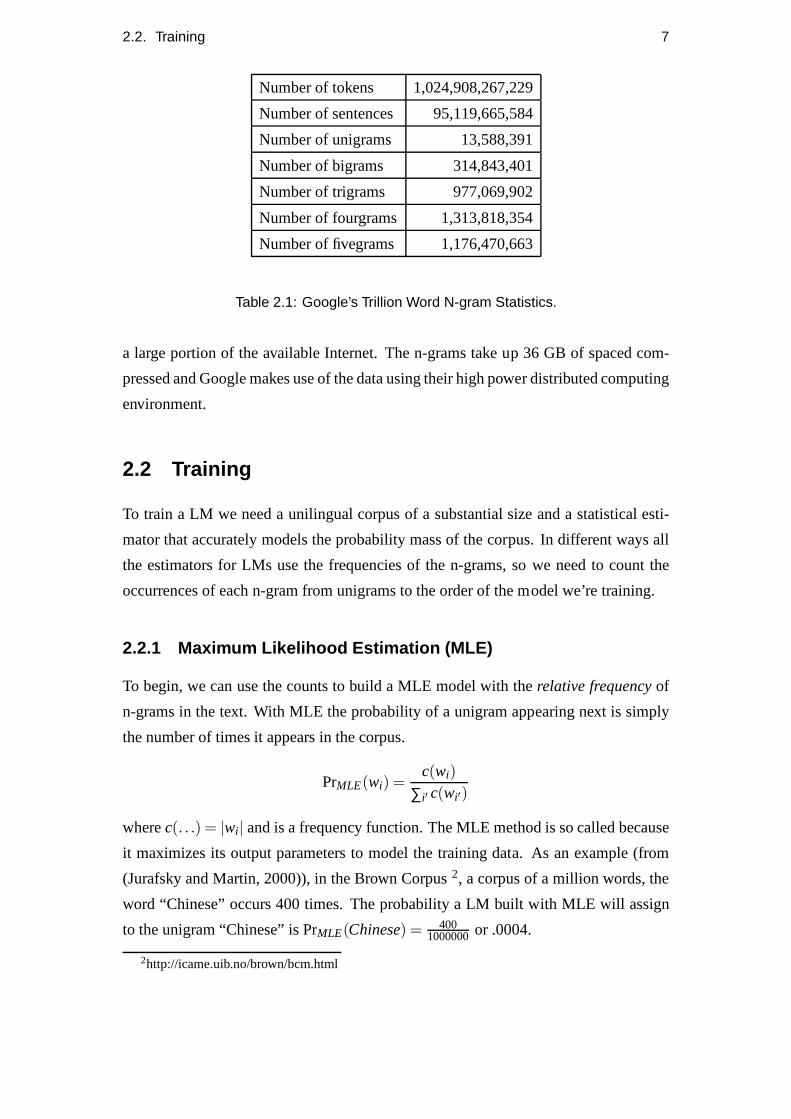
use in late 2006. The statistics of the Trillion Word N-gram set is shown in Table 2.1.
The released data set is a pruned collection from even more text stripped from crawling
1http://googleresearch.blogspot.com/2006/08/all-our- n-gram-are-belong-to-you.html
2.2. Training 7
Number of tokens 1,024,908,267,229
Number of sentences 95,119,665,584
Number of unigrams 13,588,391
Number of bigrams 314,843,401
Number of trigrams 977,069,902
Number of fourgrams 1,313,818,354
Number of fivegrams 1,176,470,663
Table 2.1: Google’s Trillion Word N-gram Statistics.
a large portion of the available Internet. The n-grams take up 36 GB of spaced com-
pressed and Google makes use of the data using their high power distributed computing
environment.
2.2 Training
To train a LM we need a unilingual corpus of a substantial sizeand a statistical esti-
mator that accurately models the probability mass of the corpus. In different ways all
the estimators for LMs use the frequencies of the n-grams, sowe need to count the
occurrences of each n-gram from unigrams to the order of the model we’re training.
2.2.1 Maximum Likelihood Estimation (MLE)
To begin, we can use the counts to build a MLE model with therelative frequencyof
n-grams in the text. With MLE the probability of a unigram appearing next is simply
the number of times it appears in the corpus.
PrMLE(wi) =c(wi)
∑i′ c(wi′)
wherec(. . .) = |wi | and is a frequency function. The MLE method is so called because
it maximizes its output parameters to model the training data. As an example (from
(Jurafsky and Martin, 2000)), in the Brown Corpus2, a corpus of a million words, the
word “Chinese” occurs 400 times. The probability a LM built with MLE will assign
to the unigram “Chinese” is PrMLE(Chinese) = 4001000000or .0004.
2http://icame.uib.no/brown/bcm.html

8 Chapter 2. Language Models
The conditional probability then for a n-gram oforder> 1 is
PrMLE(wi |wi−1i−n+1) =
c(wii−n+1)
c(wi−1i−n+1)
or the count of how often a word occurs after a certain historyof ordern−1. Continu-
ing with the above example, the probability for the bigram “Chinese food” occurring is
the number of times “food” has “Chinese” as its history divided byc(Chinese) = 400.
In the Brown corpus, “Chinese food” appears 120 times, so theraw
PrMLE( f ood|Chinese) = 0.3.
2.2.2 Smoothing
While MLE is a straight forward way of obtaining the probability model, the problem
of sparse data quickly arises in practice. Since there are aninfinite number of grammat-
ical n-grams and a LM can only contain a finite sample of these,the LM would assign
many acceptable n-grams a zero probability. To allay this problem, we step away from
MLE and use more sophisticated statistical estimators to derive the parameters. This is
calledsmoothingor discountingas we discount a fraction of the probability mass from
each event in the model and reserve the leftover mass for unseen events. What and
how much should be discounted is an active research field witha number of smoothing
algorithms available3. For example, the oldest and most straightforward isAdd-One
smoothing (de Laplace, 1996) where a constant,l ≤ 1, is added to all vocabulary
counts.
Two key concepts of smoothed LMs that were used arebackoffandinterpolation.
When the LM encounters an unknown n-gram, it may be useful to see if any of the
words in the n-gram are known events and to retrieve statistical information about
them if so. This concept is called back-off and is defined as
PrBO(wi |wi−1i−n+1) =
{
δ(wi−1i−n+1)PrLM(wi |w
i−1i−n+1) if c(wi
i−n+1) > 0
αPrBO(wii−n+2) otherwise
whereδ is a discounting factor based on the frequency of the historyandα is a back-
off penalty parameter. If we have a big enough vocabulary we may want to assign a
zero probability forout of vocabulary(OOV) words when we reach the unigram level
model. For example, we may have a domain specific vocabulary we care about or
3For an exhaustive list of smoothing algorithms and their derivations Chen and Goodman (1999,see).
2.2. Training 9
not want to remove known probability mass for OOVs such as proper nouns or real
numbers. Alternatively, we could smooth our LM so we have a small probability mass
available for OOV words and assign this to the word once we reach the unigram level.
Interpolation linearly combines the statistics of the n-gram through all the orders
of the LM. If the order of the LM isn the formula is defined recursively as
PrnI (wi |wi−1i−n+1) = λPrLM(wi |w
i−1i−n+1)+(1−λ)Prn−1
I (wi |wi−1i−n+2).
The λ parameter is a weight which we use to set which order of the LM we’d like
to impact the final outcome more. For example, we maybe trust trigram predictions
over unigram ones. Or we can baseλ on the frequency of the history. Note that the
difference between these is that interpolation uses the information from lower order
models regardless if the count is zero or not, whereas back-off does not.
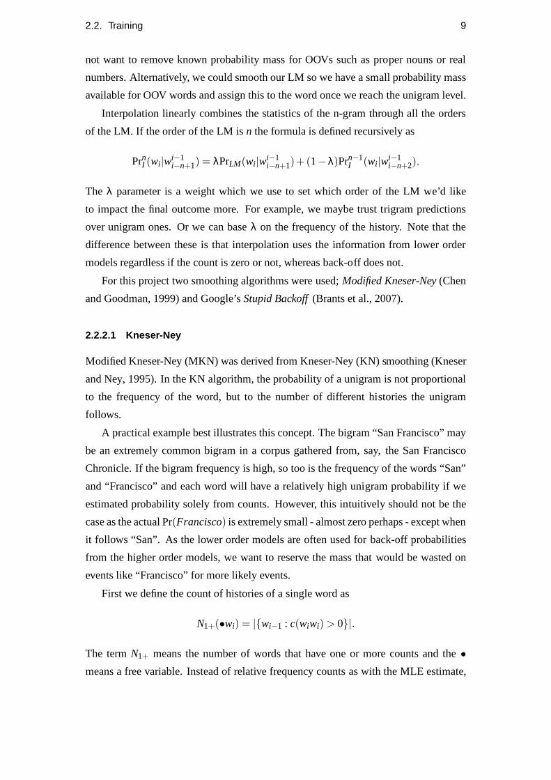
For this project two smoothing algorithms were used;Modified Kneser-Ney(Chen
and Goodman, 1999) and Google’sStupid Backoff(Brants et al., 2007).
2.2.2.1 Kneser-Ney
Modified Kneser-Ney (MKN) was derived from Kneser-Ney (KN) smoothing (Kneser
and Ney, 1995). In the KN algorithm, the probability of a unigram is not proportional
to the frequency of the word, but to the number of different histories the unigram
follows.
A practical example best illustrates this concept. The bigram “San Francisco” may
be an extremely common bigram in a corpus gathered from, say,the San Francisco
Chronicle. If the bigram frequency is high, so too is the frequency of the words “San”
and “Francisco” and each word will have a relatively high unigram probability if we
estimated probability solely from counts. However, this intuitively should not be the
case as the actual Pr(Francisco) is extremely small - almost zero perhaps - except when
it follows “San”. As the lower order models are often used forback-off probabilities
from the higher order models, we want to reserve the mass thatwould be wasted on
events like “Francisco” for more likely events.
First we define the count of histories of a single word as
N1+(•wi) = |{wi−1 : c(wiwi) > 0}|.
The termN1+ means the number of words that have one or more counts and the•
means a free variable. Instead of relative frequency countsas with the MLE estimate,
10 Chapter 2. Language Models
here the raw frequencies of words are replaced by a frequencydependent on the unique
histories proceeding the words. The KN probability for a unigram is
PrKN(wi) =N1+(•wi)
∑i′ N1+(•wi′)
or the count of the unique histories ofwi divided by the total number of unique histories
of unigrams in the corpus.
Generalizing the above for higher order models we have:
PrKN(wi |wi−1i−n+2) =
N1+(•wii−n+2)
∑i′ N1+(•wi′i′−n+2)
where the numerator
N1+(•wii−n+2) = |{wi−n+1 : c(wi
i−n+1) > 0}|
and the denominator is the sum of the count of unique histories of all n-grams the same
length ofwii−n+2. The full model of the KN algorithm is interpolated and has the form
PrKN(wi |wi−1i−n+1) =
max{c(wii−n+1−D,0}
∑i′ c(wi′i′−n+1)
+D
∑i′ c(wi′i′−n+1)
N1+(wi−1i−n+1•)PrKN(wi
i−n+2)
where
N1+(wi−1i−n+1•) = |{wi : c(wi−1
i−n+1wi) > 0}|
and is the number of unique suffixes that followwi−1i−n+1.
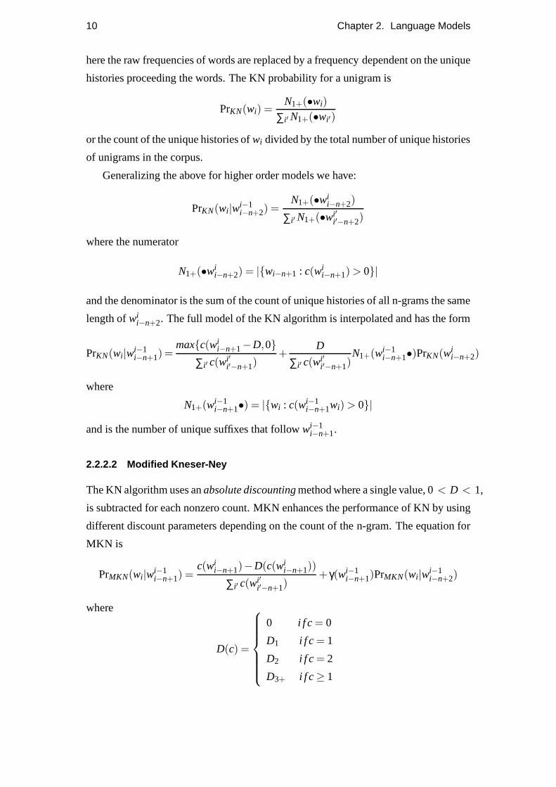
2.2.2.2 Modified Kneser-Ney
The KN algorithm uses anabsolute discountingmethod where a single value, 0< D < 1,
is subtracted for each nonzero count. MKN enhances the performance of KN by using
different discount parameters depending on the count of then-gram. The equation for
MKN is
PrMKN(wi |wi−1i−n+1) =
c(wii−n+1)−D(c(wi
i−n+1))
∑i′ c(wi′i′−n+1)
+ γ(wi−1i−n+1)PrMKN(wi |w
i−1i−n+2)
where
D(c) =
0 i f c = 0
D1 i f c = 1
D2 i f c = 2
D3+ i f c ≥ 1

2.3. Testing 11
and
Y =n1
n1+2n2
D1 = 1−2Yn2
n1
D2 = 2−3Yn3
n2
D3+ = 3−4Yn4
n3
whereni is the total number of n-grams withi counts of the higher order modeln being
interpolated. To ensure the distribution sums to one we have
γ(wi−1i−n+1) =
∑i∈{1,2,3+}DiNi(wi−1i−n+1•)
∑i′ c(wi′i′−n+1)
whereN2 andN3+ means the number of events that have two and three or more counts
respectively.
MKN has been consistently shown to have the best results of all the available
smoothing algorithms (Chen and Goodman, 1999; James, 2000).
2.2.2.3 Stupid Backoff
Google uses a simple smoothing technique, nicknamedStupid Backoff, in their dis-
tributed LM environment. The algorithm uses the relative frequencies of n-grams di-
rectly and is
S(wi |wi−1i−n+1) =
c(wii−n+1)
c(wi−1i−n+1)
if c(wiin+1) > 0
αS(wii−n+2) otherwise
whereα is a penalty parameter and is set to the constantα = 0.4. The recursion ends
once we’ve reached the unigram level probability which is just
S(wi) =wi
N
whereN is the size of the training corpus. Brants et al. (2007) claims the quality of
Stupid Backoff approaches that of MKN smoothing for large amounts of data. Note
thatS is used instead ofP to indicate that the method returns a relative score insteadof
a normalized probability.
2.3 Testing
Once a LM has been trained, we need to evaluate the quality of the model by seeing
whether the LM gives a high probability to well formed English, for example. One
12 Chapter 2. Language Models
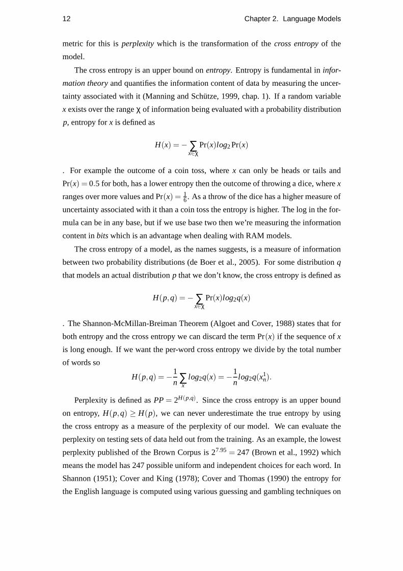
metric for this isperplexitywhich is the transformation of thecross entropyof the
model.
The cross entropy is an upper bound onentropy. Entropy is fundamental ininfor-
mation theoryand quantifies the information content of data by measuring the uncer-
tainty associated with it (Manning and Schutze, 1999, chap. 1). If a random variable
x exists over the rangeχ of information being evaluated with a probability distribution
p, entropy forx is defined as
H(x) = − ∑x∈χ
Pr(x)log2Pr(x)
. For example the outcome of a coin toss, wherex can only be heads or tails and
Pr(x) = 0.5 for both, has a lower entropy then the outcome of throwing a dice, wherex
ranges over more values and Pr(x) = 16. As a throw of the dice has a higher measure of
uncertainty associated with it than a coin toss the entropy is higher. The log in the for-
mula can be in any base, but if we use base two then we’re measuring the information
content inbitswhich is an advantage when dealing with RAM models.
The cross entropy of a model, as the names suggests, is a measure of information
between two probability distributions (de Boer et al., 2005). For some distributionq
that models an actual distributionp that we don’t know, the cross entropy is defined as
H(p,q) = − ∑x∈χ
Pr(x)log2q(x)
. The Shannon-McMillan-Breiman Theorem (Algoet and Cover,1988) states that for
both entropy and the cross entropy we can discard the term Pr(x) if the sequence ofx
is long enough. If we want the per-word cross entropy we divide by the total number
of words so
H(p,q) = −1n∑
xlog2q(x) = −
1n
log2q(x1n).
Perplexity is defined asPP= 2H(p,q). Since the cross entropy is an upper bound
on entropy,H(p,q) ≥ H(p), we can never underestimate the true entropy by using
the cross entropy as a measure of the perplexity of our model.We can evaluate the
perplexity on testing sets of data held out from the training. As an example, the lowest
perplexity published of the Brown Corpus is 27.95 = 247 (Brown et al., 1992) which
means the model has 247 possible uniform and independent choices for each word. In
Shannon (1951); Cover and King (1978); Cover and Thomas (1990) the entropy for
the English language is computed using various guessing andgambling techniques on

2.4. LMs Case Study 13
what the next letter or word will be. All reports estimate English language entropy at
around 1.3 bits per character.
The nature of a randomised LM does not guarantee correct probabilities as it rep-
resents the original data in some lossy way which skews the normal distribution. This
means we cannot use information theoretic measures such as perplexity to judge the
goodness of our lossy LMs. However, we can use a LM that does guarantee a normal
distribution and measure how far the randomised LM’s distribution deviates via both
of the LMs outputs. We can do this using the MSE between a lossless and lossy LM
over the same training and testing data. We can find the MSE unbiased estimator using
the formula
MSE=1
n−1
n
∑i(Xi −X′
i )2
whereX is the lossless LM probability of eventi andX′ is the lossy probability for the
same event.
2.4 LMs Case Study
N-gram language models are used in many NLP tasks such as speech processing, in-
formation retrieval, and optical character recognition (Manning and Schutze, 1999,
chap. 6). We illustrate briefly how a language model is used inan oversimplified
phrase-based statistical machine translation (SMT) (Koehn et al., 2003) system.
In SMT, given a source foreign languagef and a target translation languagee, we
try to maximize Pr(e| f ) for the best probable translation. Since there is never onlyone
true translation of a sentence the objective is to find the most probable sentence out of
all possible target language sentences that best represents the meaning of the foreign
sentence. We use the noisy channel approach and have
argmaxePr(e| f ) =argmaxePr( f |e)Pr(e)
Pr( f )
where Pr( f |e) is the conditional probability, Pr(e) is the prior. Pr( f ) is the marginal
probability but since it is the foreign sentence independent of e we can disregard it.
In phrase-based SMT the noisy channel formulation is turnedinto a log-linear
model in practice and weighted factors are assigned to each feature of the system
(Och and Ney, 2001). We use adecoderto decompose the source string into arbi-
trary phrases and generate a very large space of possible target language translations
for each phrase from thephrase table. The three major components of probability in

14 Chapter 2. Language Models
Figure 2.2: LM size vs. BLEU score. Training the LM with more data increases the
overall BLEU score on a log-scale.
a phrase-based SMT system are thephrase translation model, φ( f |e), the reordering
model, ωlength(e), and the LM, PrLM(e). In general we have
argmaxePr(e| f ) = argmaxe φ( f |e)λφ PrLM(e)λLM ωlength(e)λω
whereφ( f |e) is found using the probability distribution over a parallelcorpus of phrase
pairs weighted with other factors such as the length of the phrase. The reordering
modelωlength(e) constrains the distance words are allowed to travel from their original
index in the foreign sentence. Pr(e) = PrLM(e) is the LM prior the decoder uses to
score the “goodness” of the generated phrases in the target language, returning low
probabilities for unlikely n-grams and higher probabilities for likely ones.
Often the LM is assigned a higher weight than other system features because, for
example, the amount of unilingual data available to train the model is much greater than
the amount of aligned multilingual text available and so canbe “trusted” more. Och
(2005) showed that increasing the size of the LM results in log-scale improvements
in the BLEU score - a metric by which machine translated textsare scored. Figure
2.4, taken from (Koehn, 2007), shows the improvements gained by this increase in LM
size.

Chapter 3
Probabilistic Data Structures
A data set like Google’s Trillion Word N-gram is enormous and, at 24 GB when com-
pressed, too large to fit in any standard machine RAM. For a system that accesses the
LM hundreds of thousands of times per sentence, storing the set on disk memory will
result in costly IO operations that will debilitate the system’s performance. This re-
quires us to find alternative ways of representing the n-grams in the LM if we want
to gain performance from the data sets fantastic size without the traditional methods
of handling massive data sets available such as mainframes or large-scale distributed
environments such as Google’s (Brants et al., 2007).
In this chapter we explore the properties of two data structures, theBloom filter
(BF) andLossy Dictionary(LD), designed specifically forlossyrepresentation of a
set. Lossy encoding (also referred to as lossy compression)is a technique where some
amount of the data being encoded is lost but the new representation retains enough
of the original,losslessinformation to be useful when decoded. Lossy compression
techniques are common for all types of multimedia storage with JPEG for images,
MP3 for audio, and MPEG for video being well-known compression methods.
For the probabilistic data structures (PDS) we investigate, however, the data is
transformed into a lossy representation using hash functions. These data structures
are known asprobabilisticas the algorithms they support inherently use a degree of
randomness. Executing the algorithms without this measureof randomness, or deter-
ministically, would consume too much time and/or memory depending on the problem
being addressed. Instead the algorithms allow for a small probability of error as a
trade off for their speed and space savings. The algorithms can be proven to have
good performance on average with the worse case runtime being extremely unlikely
to occur. Probabilistic algorithms and their formal verification is an active research
15
16 Chapter 3. Probabilistic Data Structures
area in computer science with corollaries in many academic fields. For example see
Ravichandran et al. (2005); Hurd (2003) or the background ofthis project Talbot and
Osborne (2007a,b).
Both the BF and LD allow queries of the sort, “Isx ∈ S ?”. We call a positive
return of the query ahit and a negative return amiss. There are two types of error
returns when querying for set membership that we must concern ourselves with: false
positives and false negatives. Afalse positiveoccurs when the queried element is not a
member of the key set,x /∈ S, but is reported as a hit and an associated value is returned
in error. A false negativeis the complement to the false positive, so an elementx∈ S
is reported as a miss and no associated information is returned. A PDS that allows for
only one of these types of errors is said to have aone-sidederror while one that allows
for both types returnstwo-sidederror.
However, a LM needs to support more than just set membership queries. Frequency
values associated with keys that are in the set must be returned from the model too. The
LD supports encoding key/value pairs already, but the BF does not. However, Talbot
and Osborne (2007a) used some clever techniques to enable the support of key/value
pairs in a BF-LM. This is discussed in the next chapter.
3.1 Hash Functions
A hash functionis a function that maps data from a bit vector from one domain into
another (usually smaller) domain such that
h : U ×{0,1}w →{0,1}b.
In our discussionw is a integer that represents the bit length of a word on aunit-cost
RAM model(Hagerup, 1998). The element to be hashed comes from a setSof sizen
in a universeU such thatS⊆U andU = {0,1}w. The element’s representation in the
domainb is called asignatureor fingerprintof the data. The hash functionchopsand
mixesthe elements ofS deterministically to produce the signatures. A hash function
must be reproducible so that if the same data passes through some hash function it has
the same fingerprint every time. It must also be deterministic; if the outputs from some
hash function for two data elements are different then we know the two pieces of data
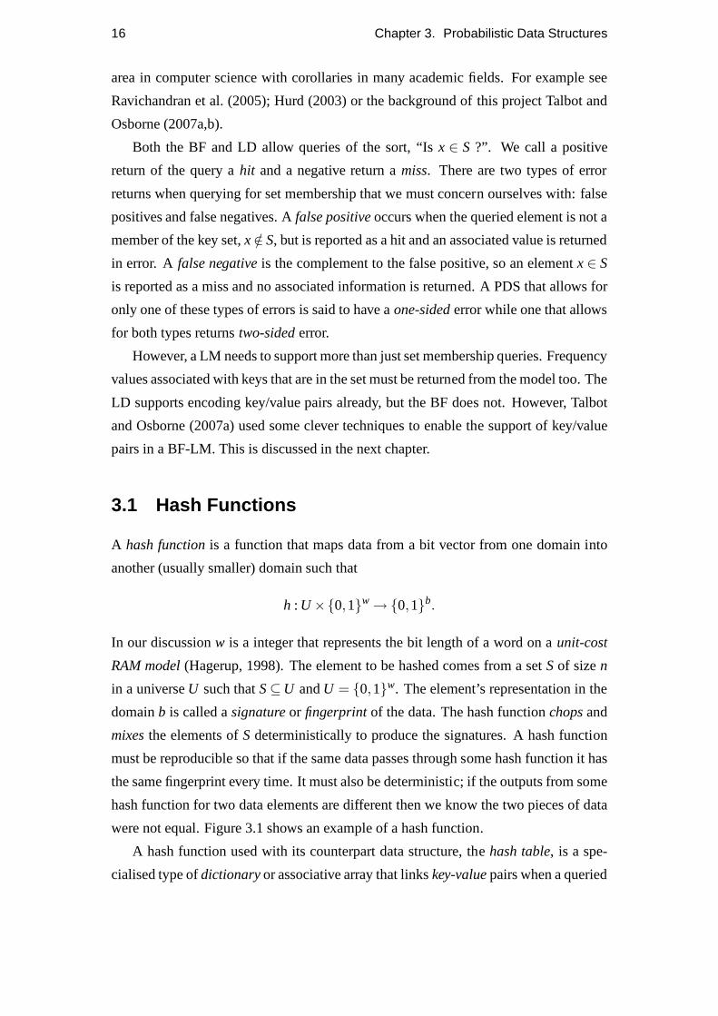
were not equal. Figure 3.1 shows an example of a hash function.
A hash function used with its counterpart data structure, the hash table, is a spe-
cialised type ofdictionaryor associative array that linkskey-valuepairs when a queried
3.1. Hash Functions 17
Figure 3.1: An example hash function in action. The strings are transformed into
hexadecimal signatures by the hash function.
item is found to be a member of the set encoded in the table. A key ki is generated
by the hash function such thath(ki) maps to a value in the range of the table size,
{0,1, . . . ,m−1}, and the associated valueai is stored in the cellh(ki). A very attrac-
tive property of a vanilla hash table is its constant look-uptime in the table regardless
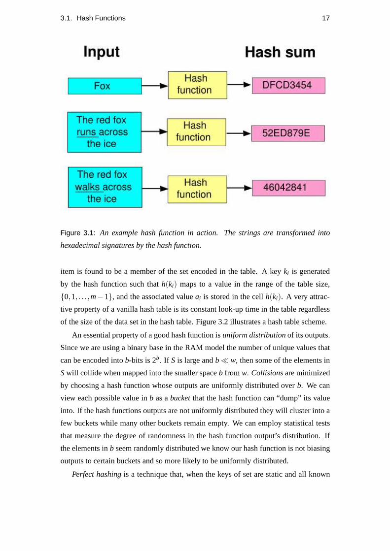
of the size of the data set in the hash table. Figure 3.2 illustrates a hash table scheme.
An essential property of a good hash function isuniform distributionof its outputs.
Since we are using a binary base in the RAM model the number of unique values that
can be encoded intob-bits is 2b. If S is large andb≪ w, then some of the elements in
Swill collide when mapped into the smaller spaceb from w. Collisionsare minimized
by choosing a hash function whose outputs are uniformly distributed overb. We can
view each possible value inb as abucketthat the hash function can “dump” its value
into. If the hash functions outputs are not uniformly distributed they will cluster into a
few buckets while many other buckets remain empty. We can employ statistical tests
that measure the degree of randomness in the hash function output’s distribution. If
the elements inb seem randomly distributed we know our hash function is not biasing
outputs to certain buckets and so more likely to be uniformlydistributed.
Perfect hashingis a technique that, when the keys of set are static and all known
18 Chapter 3. Probabilistic Data Structures
Figure 3.2: The pairs of keys ki and the associated information ai of the set S are
mapping via the hash function h into cells of the table T . The keys ki are w-bit lengths
in S and b-bit lengths in T . There is a collision between the elements k2 and k4 so the
value of ai for that cell in T is unknown.
and with a large enough number of buckets (usually of the order n2), theoretically
allows for no collisions in the hash table with probability 1/2 (Cormen et al., 2001).
However, given the size of Google’s data set, employing a perfect hashing scheme
for the LM we’re implementing is not feasible as the number ofbuckets that would
be necessary would exceed a single machine’s memory. There are other techniques
to resolve collisions, includingchaining, open addressing, andCuckoo hashing(Pagh
and Rodler, 2001a). A variant of the last technique is used inthe Lossy Dictionary
described further below.
3.1.1 Universal Hashing
One way we can minimize collisions in our hashing scheme is bychoosing a special
class of hash functionsH independent of the keys that are being stored. The hash
function parameters are chosen at random so the performanceof the hash functions
differ with each execution but we can show good performance on average. Specif-
ically, if H is a collection of finite, randomly generated hash functionswhere each
hash functionha ∈ H maps elements ofS into the range{0,1, . . . ,2b−1}, H is said to
be universalif, for all distinct keysx,y ∈ S, the number of hash functions for which

3.2. Bloom filter 19
Figure 3.3: Training and testing a Bloom filter. To train, we “turn on” k bits in the
array for each key xi . A test for membership fails if any index in the array the hash
functions map to is zero. Else we have a hit and assume membership.
h(x) = h(y)≤ |H|/2b. The corollary to this is that for a randomly chosen hash function
ha ∈ H we have theP(ha(x) = ha(y)) ≤ 1/2b for distinct keysx andy. Using a bit of
theory from numerical analysis we can quite easily generatea class of universal hash
functions for which the above is provable. (A detailed proofcan be found in Cormen
et al. (2001).)
3.2 Bloom filter
TheBloom filter(BF) (Bloom, 1970) is a PDSs that supports queries for set member-
ship. The BF has a unique encoding algorithm gives it rather spectacular space savings
at the cost of a tractable, one-sided error rate.
Before training, the BF is an array ofm bits initialized to zero. To train the BF
we needk independent hash functions (such as a family of universal hash function
described in the previous section) such that each hash function maps its output to one
of thembits in the array,hk(x) →{0,1, . . . ,m−1}. Each elementx in the setSof size
n that we’re representing with the BF is passed through each ofthe k hash functions
and the output bit in the array is set to one. So for eachx ∈ S, k bits of the array are
“turned on”. If the bit for a certainhk is already set to one from a previous element
20 Chapter 3. Probabilistic Data Structures
then it stays on. This is the source of the fantastic space advantage the BF has over
most other data structures that can encode a set - the fact that it shares the bit buckets
between the elements ofS.
To test an element for membership in the set encoded in the BF we pass it through
the samek hash functions and check the output bit of each hash functionto see if it
is turned on. If any of the bits are zero then we know for certain the element is not
a member of the set, but if each position in the bit array is setto one for all the hash
functions, then we have a hit and we assume the element is a member. However, there
is a possibility with a hit that we actually have a false positive with the same probability
that a random selection ofk bits in the array are set to one.
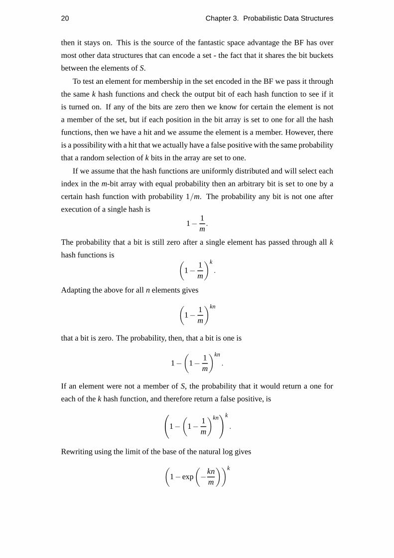
If we assume that the hash functions are uniformly distributed and will select each
index in them-bit array with equal probability then an arbitrary bit is set to one by a
certain hash function with probability 1/m. The probability any bit is not one after
execution of a single hash is
1−1m
.
The probability that a bit is still zero after a single element has passed through allk
hash functions is(
1−1m
)k
.
Adapting the above for alln elements gives
(
1−1m
)kn
that a bit is zero. The probability, then, that a bit is one is
1−
(
1−1m
)kn
.
If an element were not a member ofS, the probability that it would return a one for
each of thek hash function, and therefore return a false positive, is
(
1−
(
1−1m
)kn)k
.
Rewriting using the limit of the base of the natural log gives
(
1−exp
(
−knm
))k
3.2. Bloom filter 21
0
0.1
0.2
0.3
0.4
0.5
0.6
0.7
0.8
0.9
1
0 20000 40000 60000 80000 100000
FP
err
or r
ate
BF bits
Figure 3.4: BF error vs. space
0
0.002
0.004
0.006
0.008
0.01
0 2000 4000 6000 8000 10000
FP
err
or r
ate
# of keys
Figure 3.5: BF error vs. # keys
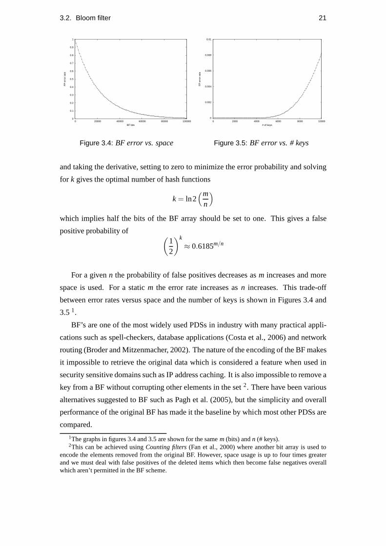
and taking the derivative, setting to zero to minimize the error probability and solving
for k gives the optimal number of hash functions
k = ln2(m
n
)
which implies half the bits of the BF array should be set to one. This gives a false
positive probability of(
12
)k
≈ 0.6185m/n
For a givenn the probability of false positives decreases asm increases and more
space is used. For a staticm the error rate increases asn increases. This trade-off
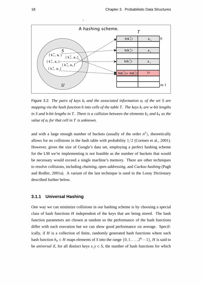
between error rates versus space and the number of keys is shown in Figures 3.4 and
3.51.
BF’s are one of the most widely used PDSs in industry with manypractical appli-
cations such as spell-checkers, database applications (Costa et al., 2006) and network
routing (Broder and Mitzenmacher, 2002). The nature of the encoding of the BF makes
it impossible to retrieve the original data which is considered a feature when used in
security sensitive domains such as IP address caching. It isalso impossible to remove a
key from a BF without corrupting other elements in the set2. There have been various
alternatives suggested to BF such as Pagh et al. (2005), but the simplicity and overall
performance of the original BF has made it the baseline by which most other PDSs are
compared.
1The graphs in figures 3.4 and 3.5 are shown for the samem (bits) andn (# keys).2This can be achieved usingCounting filters(Fan et al., 2000) where another bit array is used to
encode the elements removed from the original BF. However, space usage is up to four times greaterand we must deal with false positives of the deleted items which then become false negatives overallwhich aren’t permitted in the BF scheme.
22 Chapter 3. Probabilistic Data Structures
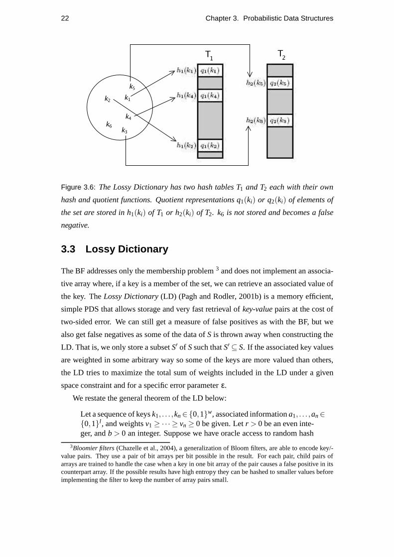
Figure 3.6: The Lossy Dictionary has two hash tables T1 and T2 each with their own
hash and quotient functions. Quotient representations q1(ki) or q2(ki) of elements of
the set are stored in h1(ki) of T1 or h2(ki) of T2. k6 is not stored and becomes a false
negative.
3.3 Lossy Dictionary
The BF addresses only the membership problem3 and does not implement an associa-
tive array where, if a key is a member of the set, we can retrieve an associated value of
the key. TheLossy Dictionary(LD) (Pagh and Rodler, 2001b) is a memory efficient,
simple PDS that allows storage and very fast retrieval ofkey-valuepairs at the cost of
two-sided error. We can still get a measure of false positives as with the BF, but we
also get false negatives as some of the data ofS is thrown away when constructing the
LD. That is, we only store a subsetS′ of Ssuch thatS′ ⊆ S. If the associated key values
are weighted in some arbitrary way so some of the keys are morevalued than others,
the LD tries to maximize the total sum of weights included in the LD under a given
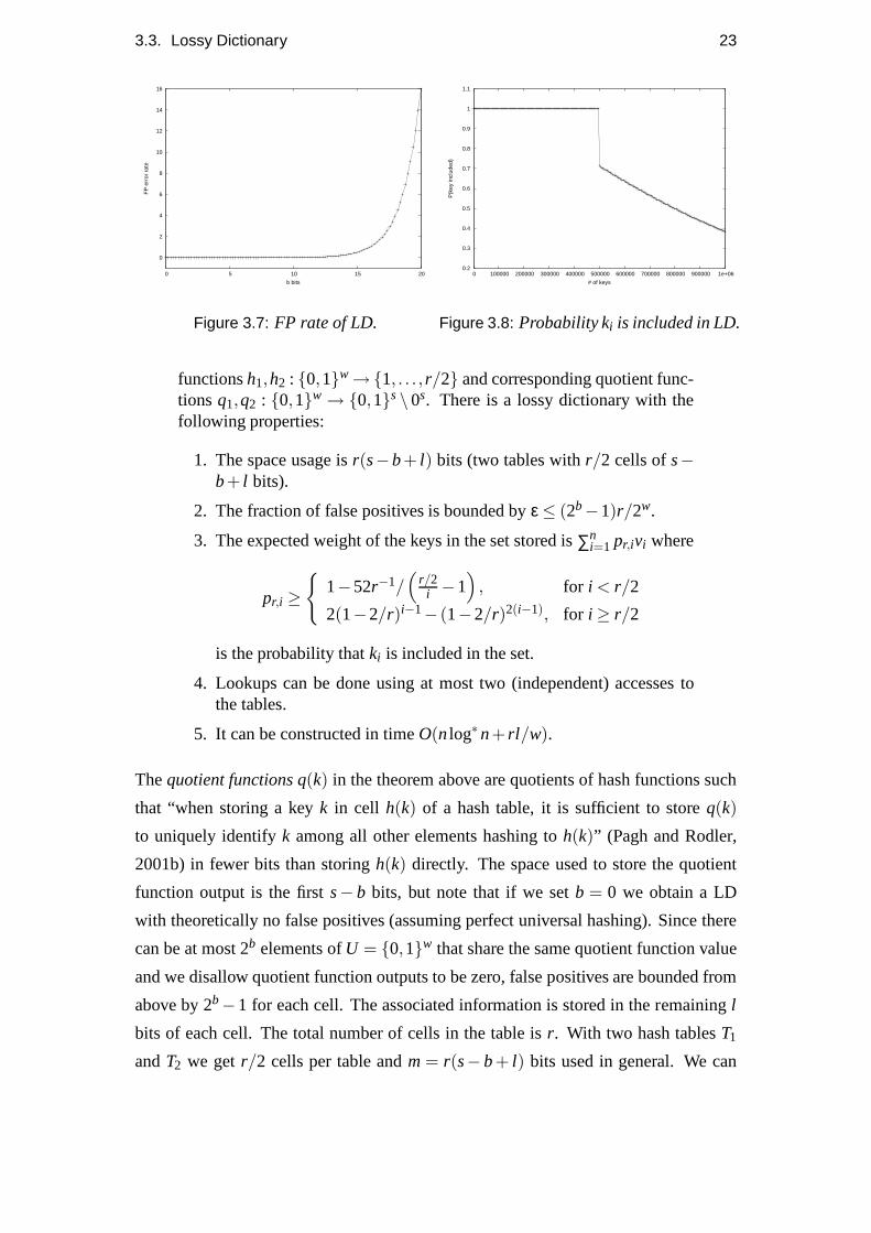
space constraint and for a specific error parameterε.
We restate the general theorem of the LD below:
Let a sequence of keysk1, . . . ,kn∈{0,1}w, associated informationa1, . . . ,an∈{0,1}l , and weightsv1 ≥ ·· · ≥ vn ≥ 0 be given. Letr > 0 be an even inte-ger, andb > 0 an integer. Suppose we have oracle access to random hash
3Bloomier filters(Chazelle et al., 2004), a generalization of Bloom filters, are able to encode key/-value pairs. They use a pair of bit arrays per bit possible in the result. For each pair, child pairs ofarrays are trained to handle the case when a key in one bit array of the pair causes a false positive in itscounterpart array. If the possible results have high entropy they can be hashed to smaller values beforeimplementing the filter to keep the number of array pairs small.
3.3. Lossy Dictionary 23
0
2
4
6
8
10
12
14
16
0 5 10 15 20
FP
err
or r
ate
b bits
Figure 3.7: FP rate of LD.
0.2
0.3
0.4
0.5
0.6
0.7
0.8
0.9
1
1.1
0 100000 200000 300000 400000 500000 600000 700000 800000 900000 1e+06
P(k
ey in
clud
ed)
# of keys
Figure 3.8: Probability ki is included in LD.
functionsh1,h2 : {0,1}w →{1, . . . , r/2} and corresponding quotient func-tions q1,q2 : {0,1}w → {0,1}s\0s. There is a lossy dictionary with thefollowing properties:
1. The space usage isr(s−b+ l) bits (two tables withr/2 cells ofs−b+ l bits).
2. The fraction of false positives is bounded byε ≤ (2b−1)r/2w.
3. The expected weight of the keys in the set stored is∑ni=1 pr,ivi where
pr,i ≥
{
1−52r−1/(
r/2i −1
)
, for i < r/2
2(1−2/r)i−1− (1−2/r)2(i−1), for i ≥ r/2
is the probability thatki is included in the set.
4. Lookups can be done using at most two (independent) accesses tothe tables.
5. It can be constructed in timeO(nlog∗n+ rl /w).
Thequotient functions q(k) in the theorem above are quotients of hash functions such
that “when storing a keyk in cell h(k) of a hash table, it is sufficient to storeq(k)
to uniquely identifyk among all other elements hashing toh(k)” (Pagh and Rodler,
2001b) in fewer bits than storingh(k) directly. The space used to store the quotient
function output is the firsts− b bits, but note that if we setb = 0 we obtain a LD
with theoretically no false positives (assuming perfect universal hashing). Since there
can be at most 2b elements ofU = {0,1}w that share the same quotient function value
and we disallow quotient function outputs to be zero, false positives are bounded from
above by 2b−1 for each cell. The associated information is stored in the remainingl
bits of each cell. The total number of cells in the table isr. With two hash tablesT1
andT2 we getr/2 cells per table andm= r(s− b+ l) bits used in general. We can

24 Chapter 3. Probabilistic Data Structures
choose optimalr given a predetermined maximum errorε and space usagem. Figure
3.6 (in part from Pagh and Rodler (2001b)) shows the overall structure of the LD.
To train the LD, we use the following greedy algorithm:
1. Initialize a union-find data structure for the cells of thehash tables.
2. For each equivalence class, set a “saturated” flag to false.
3. Fori = 1, . . . ,n:
(a) Find the equivalence classcb of each cellhb(ki) in Tb, for b = 1,2.
(b) If c1 or c2 is not saturated:
i. Includeki in the solution.
ii. Join c1 andc2 to form an equivalence classc.
iii. Set the saturated flag ofc if c1 = c2 of if the flag is set forc1 or c2.
In practice, we simply hash an elementki into the cellh1(ki) of T1. If the cellT1[h1(ki)]
is empty we storeq1(ki) and the associated valuevi in it and we’re finished. Else
we repeat the process forh2(ki) of T2. If the cell in T2 is not empty,ki is discarded
and included in the subset of false negatives. Figure 3.8 shows the probability of a
key being included in the tables from a set of size one million. For i < r/2 we keep
almost all the keys with almost certain probability, but fori ≥ r/2 the probability of a
key being included drops sharply throughout. We examine this property empirically in
chapter four.
During testing a similar process is repeated. We hash a test elementki with h1 and
get the quotient value. If the value inT1[h1(ki)] = q1(ki) we assume a hit and retrieve
the associated valuevi . If it doesn’t match we hashki throughh2 andq2 and check for
a match inT2. If the equality fails, we report a miss which may or may not bea false
negative.
3.4 Comparison
The LD uses the RAM approach for storing and accessing information which processes
bits in groups ofwords. The theoretic word model uses units of computation in binary
base{0,1}w which simulates a processor where bits are compared in word sizesw that
range from 23 (8-bit) up to 27 (128-bit) normally. The BF, on the other hand, uses a

3.4. Comparison 25
boolean model which requires more computing time to comparethe same number of
bits that an LD can do with one bucket comparison.
As stated, the BF doesn’t support associated key/value pairs as each bit is accessed
in isolation and is either on and a member of the set or off and not a member. There
are no other values possible in a boolean setting. When we usethe unit-cost RAM
model we group a pair of bit-buckets or divide a bucket into various sub-buckets that
can easily represent associated key/value data. This is theunderlying cause of the
space advantage the BF has between the two PDSs as well since the word-based RAM
modelsmustuse a certain minimum number of bits for each item in the data set. The
RAM model can’t share bits among the keys it is encoding like the BF does as once a
word bucket is setup to represent a key from the set, adding orchanging the bits in it
will destroy the information for the originally contained key. Once the BF is setup, it
also can’t change bits arbitrarily without potentially destroying information related to
multiple keys. In this way the BF can be envisioned as a singlegiant bucket which is
trained to represent the whole space between the bits and it derives it’s space advantage
over the LD from this.
The probability of error for each structure depends specifically on the data set and
free variable parameter settings such as the space bounds orencoding scheme used for
the buckets in the LD. But the BF’s one-sided error is an advantage compared with the
two-sided error of the LD which can return both false negatives and false positives so
we can say that all things being equal the BF has lower error returns than the LD.

Chapter 4
Previous Work
The previous work and basis for this project was the groundbreaking work published
by Talbot and Osborne (2007a) and Talbot and Osborne (2007b). The research reported
in these papers was the first time a randomised data structuresuch as a BF was used
to encode a LM and some very clever ideas were used to minimizethe false positive
returns and enable the BF to support key-value pairs rather than just set membership
queries.
To train the BF as a data structure that supports key-value pairs, where the key
is the n-gram and the value is the count of that n-gram in the corpus, the value was
appended to the key before entering this composite event into the BF. To minimise the
number of bits needed for the frequency value alog-frequencyencoding scheme was
used. The n-gram counts were first quantized by using a logarithmic codebook so the
actual countc(x) of the n-gram was represented as a quantized countqc(x) such that
qc(x) = 1+ ⌊logbc(x)⌋.
The accuracy of this codebook relies on the Zipf distribution of the n-grams where
a few events occur frequently but most events occur only a small number of times.
For the high-end of the Zipf distribution the counts in the BF-LM are exponentially
decayed using the log-frequency scheme. However, the largegap in distribution of
these events means that a ratio of the likelihood of the modelwas preserved in the
BF-LM.
To keep it tractable as well as minimize the false positive probability the com-
posite events of n-grams and their quantised counts were entered into the BF using
sub-sequence filtering. With sub-sequence filtering, each n-gram was entered into the
BF with attached counts from one up to the value ofqc(x) for that n-gram. During
27
28 Chapter 4. Previous Work
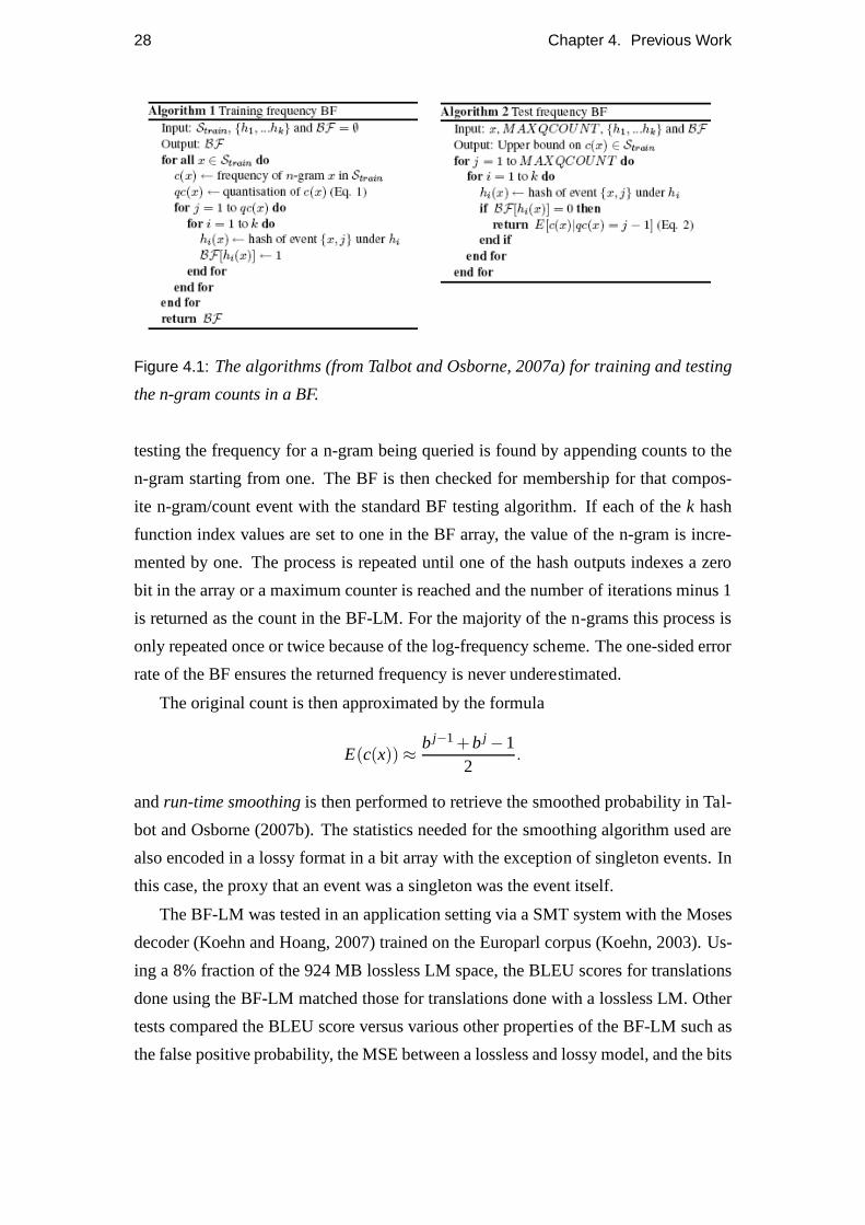
Figure 4.1: The algorithms (from Talbot and Osborne, 2007a) for training and testing
the n-gram counts in a BF.
testing the frequency for a n-gram being queried is found by appending counts to the
n-gram starting from one. The BF is then checked for membership for that compos-
ite n-gram/count event with the standard BF testing algorithm. If each of thek hash
function index values are set to one in the BF array, the valueof the n-gram is incre-
mented by one. The process is repeated until one of the hash outputs indexes a zero
bit in the array or a maximum counter is reached and the numberof iterations minus 1
is returned as the count in the BF-LM. For the majority of the n-grams this process is
only repeated once or twice because of the log-frequency scheme. The one-sided error
rate of the BF ensures the returned frequency is never underestimated.
The original count is then approximated by the formula
E(c(x)) ≈b j−1+b j −1
2.
andrun-time smoothingis then performed to retrieve the smoothed probability in Tal-
bot and Osborne (2007b). The statistics needed for the smoothing algorithm used are
also encoded in a lossy format in a bit array with the exception of singleton events. In
this case, the proxy that an event was a singleton was the event itself.
The BF-LM was tested in an application setting via a SMT system with the Moses
decoder (Koehn and Hoang, 2007) trained on the Europarl corpus (Koehn, 2003). Us-
ing a 8% fraction of the 924 MB lossless LM space, the BLEU scores for translations
done using the BF-LM matched those for translations done with a lossless LM. Other
tests compared the BLEU score versus various other properties of the BF-LM such as
the false positive probability, the MSE between a lossless and lossy model, and the bits

29
used per n-gram. Though the space savings were quite spectacular, the BF-LM is a
slow data structure due to the number of hashes used to support the bit-sharing as well
as the added hashes for the sub-sequencing to support key/value pairs. In average the
translation time took between 2–5 times longer when a BF-LM was used.
This work provided the first complete framework for using randomised data struc-
ture LMs in NLP and was the basis of investigation for this project.

Chapter 5
Testing Framework
This chapter describes the testing framework we used to testour lossy LMs. An
overview of the framework’s structure is shown in figure 5.1.
5.1 Overview
We implemented lossy language models using the BF-LM from Talbot and Osborne
(2007a) and a lossy dictionary LM (LD-LM) using various encoding schemes. We
can’t use perplexity or cross-entropy to measure the goodness of a lossy LM as the
error returns may skew the distribution and report better than actual results. Instead,
since we can be sure that the reported perplexity and probabilities from the lossless
LM are correct, we used SRILM Stolcke (2002) to train a lossless LM and used its
output as a gold standard to measure the performance of our lossy LMs. Specifically,
we used the mean squared error (MSE) of the per sentence difference between the log-
probabilities of our lossy LMs and SRILM’s output. We aim to minimize the MSE
throughout our experiments.
5.2 Training Data
For training the same corpus was always used for both lossy and lossless LMs. After
initial setup and testing with just a few sentences, a mediumsized corpus of 3.5 million
words and 1.8 million unique n-grams that comes with the SRILM source was used for
training during the bulk of the experiments. Final tests were done with the 110 million
word British National Corpus1.
1http://www.natcorp.ox.ac.uk/
31
32 Chapter 5. Testing Framework
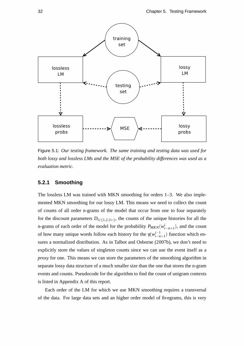
Figure 5.1: Our testing framework. The same training and testing data was used for
both lossy and lossless LMs and the MSE of the probability differences was used as a
evaluation metric.
5.2.1 Smoothing
The lossless LM was trained with MKN smoothing for orders 1–3. We also imple-
mented MKN smoothing for our lossy LM. This means we need to collect the count
of counts of all order n-grams of the model that occur from oneto four separately
for the discount parametersDi∈{1,2,3+}, the counts of the unique histories for all the
n-grams of each order of the model for the probabilityPMKN(wii−n+1), and the count
of how many unique words follow each history for theγ(wi−1i−n+1) function which en-
sures a normalized distribution. As in Talbot and Osborne (2007b), we don’t need to
explicitly store the values of singleton counts since we canuse the event itself as a
proxy for one. This means we can store the parameters of the smoothing algorithm in
separate lossy data structure of a much smaller size than theone that stores the n-gram
events and counts. Pseudocode for the algorithm to find the count of unigram contexts
is listed in Appendix A of this report.
Each order of the LM for which we use MKN smoothing requires a transversal
of the data. For large data sets and an higher order model of fivegrams, this is very
5.3. Testing Data 33
time and resource consuming to do repeatedly. During our experiments, since we were
purely testing the information content and properties of the data structures encoding
the LM and not interested in the precise probabilities of theevents themselves, we
used Google’s Stupid Backoff smoothing algorithm for the lossy LMs because of its
speed and simplicity. An extremely small part of the difference in the outputs between
the lossless and lossy LMs stemmed from the different smoothing techniques used
between the gold standard SRILM output and our lossy LMs, butas this was a constant
factor between the lossy data structures we could safely ignore it.
To use the smoothed probabilities during testing we split each test sentence into
tokens and surrounded the first and last of them with begin (<s>) and end (</s>) sen-
tence markers respectively. To extract the n-grams in the sentence we iterate through
each word index of the sentence adding the histories of the word starting from the
highest order length of the model and working towards the word we’re finding the con-
ditional probability for. For Stupid Backoff we’d pickup backoff probabilities as we
built the n-gram and clear them if the full order n-gram was found in the LM since it
isn’t an interpolated algorithm. For MKN, we found the backoff and recursed until we
reached the unigram level at which point we’d pick up the fulln-gram probabilities,
add them to the backoffs and return through the stack. The algorithms for smoothed
probability retrieval are listed in full in Appendix A.
5.3 Testing Data
To test our lossy LMs for perplexity we used clean text of 5290more or less gram-
matical sentences. However, in an application environmentsuch as SMT most of the
n-grams being passed to the LM by the decoder are rubbish. To simulate this we gen-
erated multiple completely randomised text files of varyinglength and tested the LMs
with these as well. For all the results of the experiments shown in this chapter we have
taken the average of the results of multiple tests on both theperplexity data file and
arbitrary randomized n-gram files unless specified otherwise. As well, the tests that
compare the PDS LMs were always executed with the same instantiation of the hash
function family.
34 Chapter 5. Testing Framework
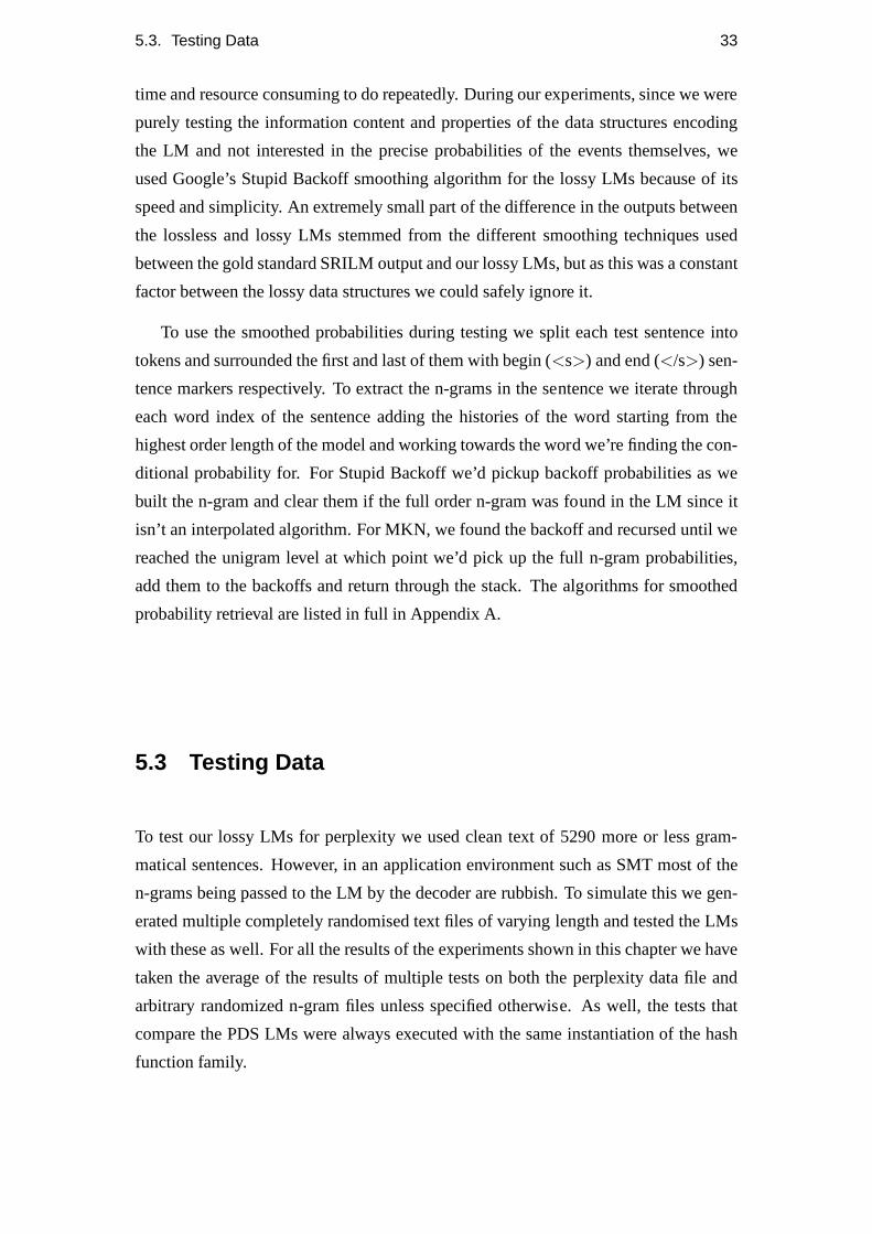
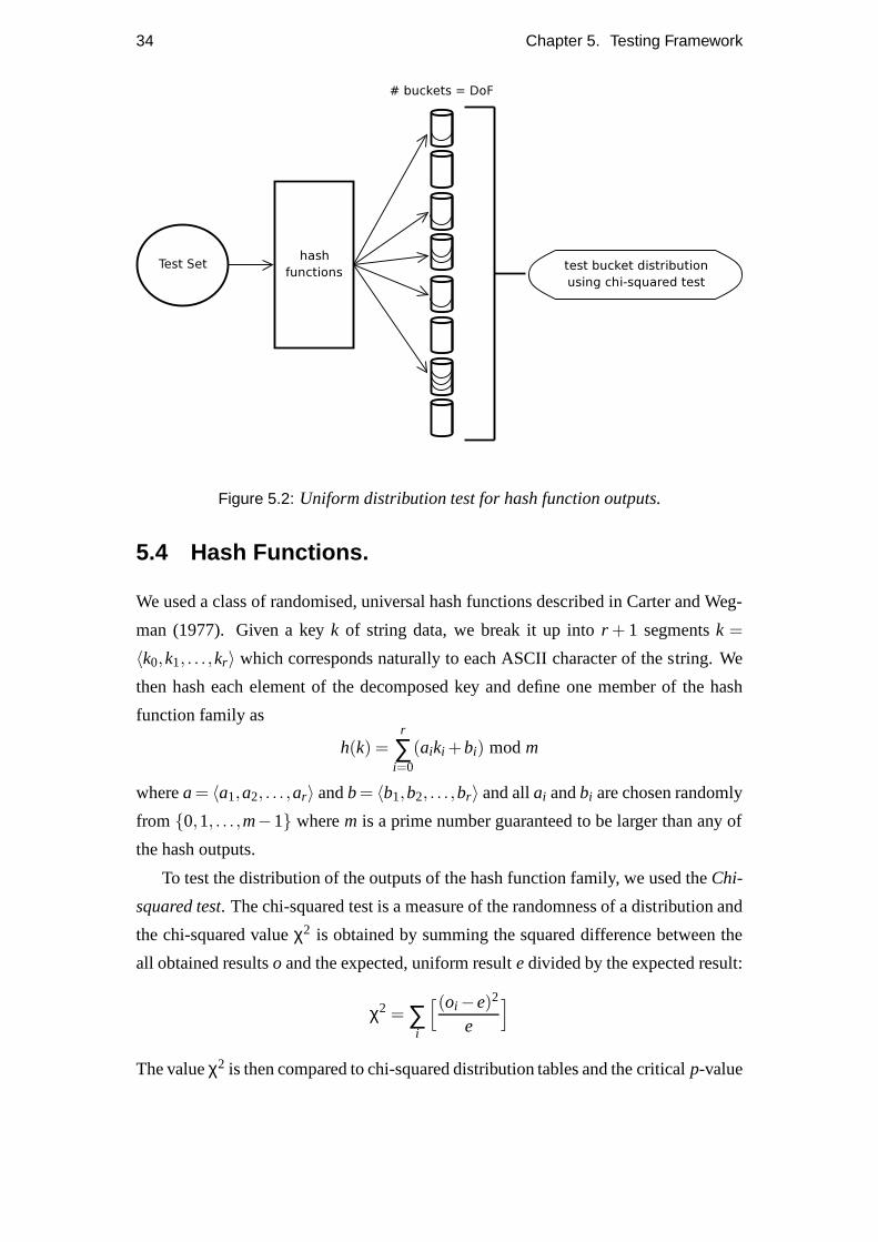
Figure 5.2: Uniform distribution test for hash function outputs.
5.4 Hash Functions.
We used a class of randomised, universal hash functions described in Carter and Weg-
man (1977). Given a keyk of string data, we break it up intor + 1 segmentsk =
〈k0,k1, . . . ,kr〉 which corresponds naturally to each ASCII character of the string. We
then hash each element of the decomposed key and define one member of the hash
function family as
h(k) =r
∑i=0
(aiki +bi) modm
wherea= 〈a1,a2, . . . ,ar〉 andb= 〈b1,b2, . . . ,br〉 and allai andbi are chosen randomly
from {0,1, . . . ,m−1} wherem is a prime number guaranteed to be larger than any of
the hash outputs.
To test the distribution of the outputs of the hash function family, we used theChi-
squared test. The chi-squared test is a measure of the randomness of a distribution and
the chi-squared valueχ2 is obtained by summing the squared difference between the
all obtained resultso and the expected, uniform resultedivided by the expected result:
χ2 = ∑i
[(oi −e)2
e
]
The valueχ2 is then compared to chi-squared distribution tables and thecritical p-value

5.4. Hash Functions. 35
is obtained as a function of the degrees of freedom of the distribution. We maintained
randomness of the distribution if our critical valuep > 0.05.
Our hash function outputs were designed to range between 16-bit outputs (216) to
arbitrarily high values (though ranging beyond 264 values is superfluous even for the
trillion word data set). We split the test up between the lower and upper halves of the
output bits and measured the distribution of each half. Eachelement of the test data
was hashed by a randomly chosen member of our universal hash family and the hash
value bit-masked and right-shifted (for the upper half) to split the upper and lower half
of the bits. Then the index of the hash values in a representative data structure was
incremented and, after all elements had been hashed and bucketed, the chi-squared
distribution was performed for both halves. If both the upper and lower half distri-
butions were randomly distributed separately then they were random together as well
but if many outputs were written to the same subset of the buckets the chi-squared
test would show the hash outputs as not being randomised and we could expect high
collisions for the chosen hash family (Mulvey, 2006).
We ran a total of 500 tests over 3 million elements for 16, 32, and 64-bit outputs,
concentrating mostly on the higher bit outputs. Only twice was the criticalp-value<
0.05 which was the expected result that, with near certainty, the universal class of hash
function’s outputs were random and uniformly distributed.


Chapter 6
Experiments
In this chapter we focus on the experiments conducted over the course of the research
and the empirical results of the experiments. This chapter also reports the findings of
the first known use of a Lossy Dictionary to implement a language model. Since the
LD has many free variables associated with it, there are a lotof parameters we can
fiddle with and a number of variations of LD-LM we examine.
6.1 Baseline LD-LM
Our LD-LM baseline was the first attempt at using a LD for a LM and we tried a novel
approach. Instead of encoding just the n-gram events and their associated counts, asub-
bucketscheme was used to try and include a smoothed LM representation in the LD
tables with no run-time smoothing. Our hope was to create a proper ratio of a lossless
LM in the LD-LM using this scheme so no runtime smoothing would be needed.
The sub-bucket encoding scheme is shown in figure 6.1. Our LD stored all the
information for a n-gram in just one cell unlike a traditional hash table which uses one
cell for the hash signature and a conceptually adjacent cellfor the associated informa-
tion. Using just once cell per bucket saves a considerable amount of space and makes
the division of a pre-defined space parameter easier to manipulate. For our baseline
each table cell was divided in 3 sub-buckets. For example, ifa table cell was 16-bits,
we use a 8-4-4 sub-bucket scheme where the first sub-bucket ofthe 8 most significant
bits (MSB) would be used for the quotient signature1 of the n-gram, the next 4 bits to
encode a quantized value of the probability and the least significant 4 bits remaining
1The quotient functions were another family of hash functions with the added stipulation that nooutput could be zero.
37
38 Chapter 6. Experiments
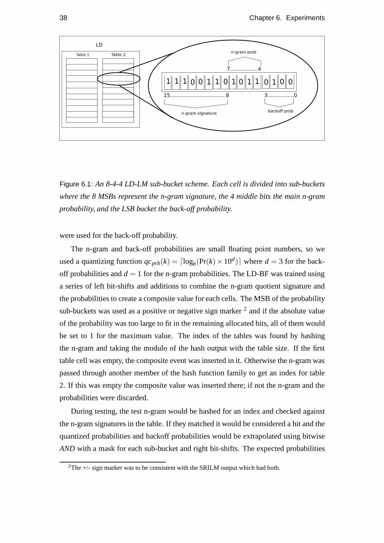
Figure 6.1: An 8-4-4 LD-LM sub-bucket scheme. Each cell is divided into sub-buckets
where the 8 MSBs represent the n-gram signature, the 4 middlebits the main n-gram
probability, and the LSB bucket the back-off probability.
were used for the back-off probability.
The n-gram and back-off probabilities are small floating point numbers, so we
used a quantizing functionqcprb(k) = ⌈logb(Pr(k)×10d)⌉ whered = 3 for the back-
off probabilities andd = 1 for the n-gram probabilities. The LD-BF was trained using
a series of left bit-shifts and additions to combine the n-gram quotient signature and
the probabilities to create a composite value for each cells. The MSB of the probability
sub-buckets was used as a positive or negative sign marker2 and if the absolute value
of the probability was too large to fit in the remaining allocated bits, all of them would
be set to 1 for the maximum value. The index of the tables was found by hashing
the n-gram and taking the modulo of the hash output with the table size. If the first
table cell was empty, the composite event was inserted in it.Otherwise the n-gram was
passed through another member of the hash function family toget an index for table
2. If this was empty the composite value was inserted there; if not the n-gram and the
probabilities were discarded.
During testing, the test n-gram would be hashed for an index and checked against
the n-gram signatures in the table. If they matched it would be considered a hit and the
quantized probabilities and backoff probabilities would be extrapolated using bitwise
AND with a mask for each sub-bucket and right bit-shifts. The expected probabilities
2The +/- sign marker was to be consistent with the SRILM outputwhich had both.

6.1. Baseline LD-LM 39
were recovered using the formula Pr(k) = b j/10d where j was the number retrieved
from the encoded value in the cell. Example pseudocode for the algorithms to insert
a value into a cell of the LD and retrieve the probabilities during testing are listed in
Appendix A.
Figure 6.2 shows the percentage of the original data set thatwas contained in the
LD as a function of the space parameter in megabytes (MB) for 8and 16-bit cell sizes.
With 16-bit cells and 1 MB of space we keep only 30% of the data,but at 10 MB
97% of the data is retained in the LD. If we use 8-bit cells, since we have double the
number of table cells we keep a higher percentage of the data for a smaller table size.
Obviously, we also lose half the information storage per event. In comparison, the
lossless LM for our small training set used 34.99 MBs to storethe whole set.
0
20
40
60
80
100
0 2 4 6 8 10
% o
f dat
a ke
pt
MB
% of data kept in LD
16-bit LD8-bit LD
32-bit LD(SRILM 34.99 MB)
Figure 6.2: The percentage of the original data set kept in the LD-LM as the size
increases in MB. The lossless LM for this set of training datais stored at 35 MB.
The graph in figure 6.3 shows the inverse relation to the percentage of the data kept
which is the number of collisions for different space settings. As more space is given
the number of collisions decrease until, for an amount of space that is far beyond what
is necessary for the items in the space, we have a limit of zerocollisions. We can
tell from this that most collisions don’t come from a large number of n-grams being
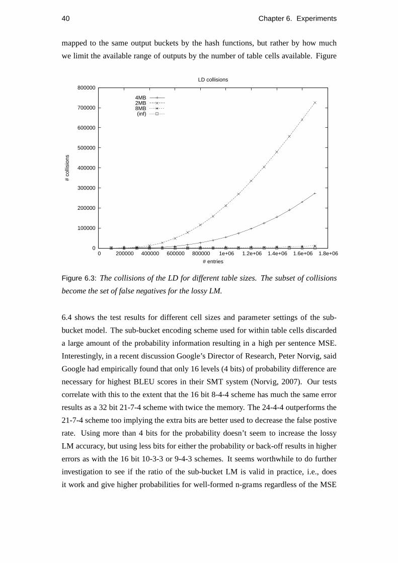
40 Chapter 6. Experiments
mapped to the same output buckets by the hash functions, but rather by how much
we limit the available range of outputs by the number of tablecells available. Figure
0
100000
200000
300000
400000
500000
600000
700000
800000
0 200000 400000 600000 800000 1e+06 1.2e+06 1.4e+06 1.6e+06 1.8e+06
# co
llisi
ons
# entries
LD collisions
4MB2MB8MB(inf)
Figure 6.3: The collisions of the LD for different table sizes. The subset of collisions
become the set of false negatives for the lossy LM.
6.4 shows the test results for different cell sizes and parameter settings of the sub-
bucket model. The sub-bucket encoding scheme used for within table cells discarded
a large amount of the probability information resulting in ahigh per sentence MSE.
Interestingly, in a recent discussion Google’s Director ofResearch, Peter Norvig, said
Google had empirically found that only 16 levels (4 bits) of probability difference are
necessary for highest BLEU scores in their SMT system (Norvig, 2007). Our tests
correlate with this to the extent that the 16 bit 8-4-4 schemehas much the same error
results as a 32 bit 21-7-4 scheme with twice the memory. The 24-4-4 outperforms the
21-7-4 scheme too implying the extra bits are better used to decrease the false postive
rate. Using more than 4 bits for the probability doesn’t seemto increase the lossy
LM accuracy, but using less bits for either the probability or back-off results in higher
errors as with the 16 bit 10-3-3 or 9-4-3 schemes. It seems worthwhile to do further
investigation to see if the ratio of the sub-bucket LM is valid in practice, i.e., does
it work and give higher probabilities for well-formed n-grams regardless of the MSE
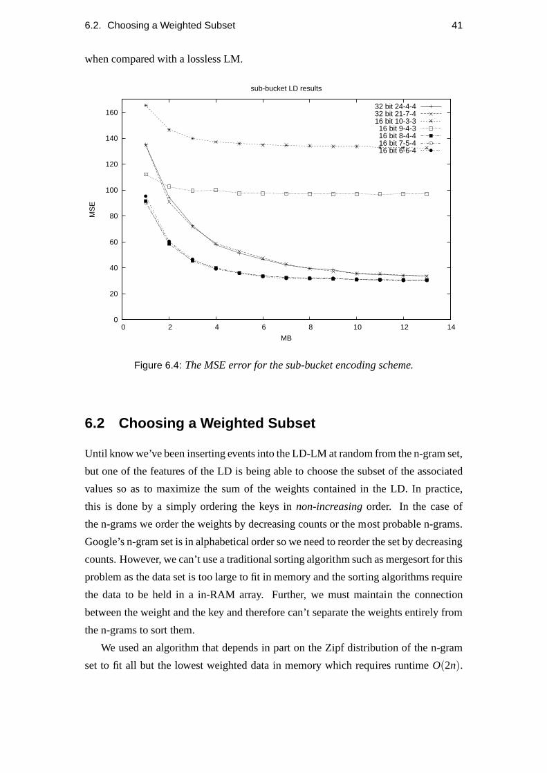
6.2. Choosing a Weighted Subset 41
when compared with a lossless LM.
0
20
40
60
80
100
120
140
160
0 2 4 6 8 10 12 14
MS
E
MB
sub-bucket LD results
32 bit 24-4-432 bit 21-7-416 bit 10-3-3
16 bit 9-4-316 bit 8-4-416 bit 7-5-416 bit 6-6-4
Figure 6.4: The MSE error for the sub-bucket encoding scheme.
6.2 Choosing a Weighted Subset
Until know we’ve been inserting events into the LD-LM at random from the n-gram set,
but one of the features of the LD is being able to choose the subset of the associated
values so as to maximize the sum of the weights contained in the LD. In practice,
this is done by a simply ordering the keys innon-increasingorder. In the case of
the n-grams we order the weights by decreasing counts or the most probable n-grams.
Google’s n-gram set is in alphabetical order so we need to reorder the set by decreasing
counts. However, we can’t use a traditional sorting algorithm such as mergesort for this
problem as the data set is too large to fit in memory and the sorting algorithms require
the data to be held in a in-RAM array. Further, we must maintain the connection
between the weight and the key and therefore can’t separate the weights entirely from
the n-grams to sort them.
We used an algorithm that depends in part on the Zipf distribution of the n-gram
set to fit all but the lowest weighted data in memory which requires runtimeO(2n).

42 Chapter 6. Experiments
On the first pass weprefix count the number of each unique weight associated with
the keys in the set, i.e. every unique weight has the count of the number of events
with its same weight plus the sum of the keys with weight greater than its own. We
store this number in a sorted dictionary structure called amapin C++. The keys of the
map are the weights and the values are the prefix counts of all events in the n-gram set
with that weight. On the second pass we store n-grams with counts>1 in an array in
RAM memory with n-gram at the index in this array of the prefix count of the n-gram’s
weight. Then we subtract one from that weights prefix count inthe map for the index
of the next key in the set with the same weight. In this way we fill in the slots of the
array so finally we end up with an array of n-grams in decreasing order. We write all
events with the lowest weights out to static memory until allother prefix counts are
zero. After, when we’re training the LM, we first use the non-increasing array in RAM
memory and then add the singleton events of lower weight in arbitrary order from the
singleton file. This sorting algorithm’s pseudocode is listed in Appendix A.
Once the weights are ordered in non-increasing order, the subset that is included
in the LD will be the maximum subset able to be included given the hash function set
and the size of the tables. Figure 6.5 show how ordering the data effects the results
for the MSE of the sub-bucket scheme. Note that we use the smoothed probabilities
as our weight metric for the most valued n-grams in the sub-bucket scheme. Since the
higher order n-grams of the model usually have a greater smoothed probability mass
associated with them compared to lower order n-grams, they’re are at the beginning of
the ordered set and therefore are included in the LD-LM with very high probability.
However, these n-grams don’t have backoff weights associated with them as no higher
order model exists that will backoff to them since they are the highest order of the
LM. Without ordering, the unigrams and bigrams with lower probability mass but also
backoff mass are entered first and most of them end up in the LD-LM. This trade-off
is a draw back of the sub-bucket scheme that with tight space bounds we lose much of
the smoothed backoff probability mass in the ordered LD whenincluding the highest
weighted subset. We examine the effect of choosing the highest weighted subset on
the MSE using the n-grams frequencies in experiment 4.
6.3 BF-LM
We implemented the BF-LM from Talbot and Osborne (2007a) described in back-
ground Sect. 4 of this report for our next experiment. For training, the n-grams and
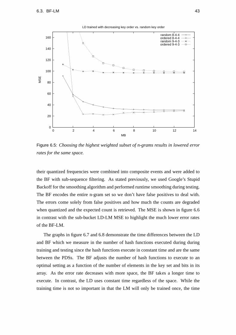
6.3. BF-LM 43
0
20
40
60
80
100
120
140
160
0 2 4 6 8 10 12 14
MS
E
MB
LD trained with decreasing key order vs. random key order
random 8-4-4ordered 8-4-4random 9-4-3ordered 9-4-3
Figure 6.5: Choosing the highest weighted subset of n-grams results in lowered error
rates for the same space.
their quantized frequencies were combined into composite events and were added to
the BF with sub-sequence filtering. As stated previously, weused Google’s Stupid
Backoff for the smoothing algorithm and performed runtime smoothing during testing.
The BF encodes the entire n-gram set so we don’t have false positives to deal with.
The errors come solely from false positives and how much the counts are degraded
when quantized and the expected count is retrieved. The MSE is shown in figure 6.6
in contrast with the sub-bucket LD-LM MSE to highlight the much lower error rates
of the BF-LM.
The graphs in figure 6.7 and 6.8 demonstrate the time differences between the LD
and BF which we measure in the number of hash functions executed during during
training and testing since the hash functions execute in constant time and are the same
between the PDSs. The BF adjusts the number of hash functionsto execute to an
optimal setting as a function of the number of elements in thekey set and bits in its
array. As the error rate decreases with more space, the BF takes a longer time to
execute. In contrast, the LD uses constant time regardless of the space. While the
training time is not so important in that the LM will only be trained once, the time
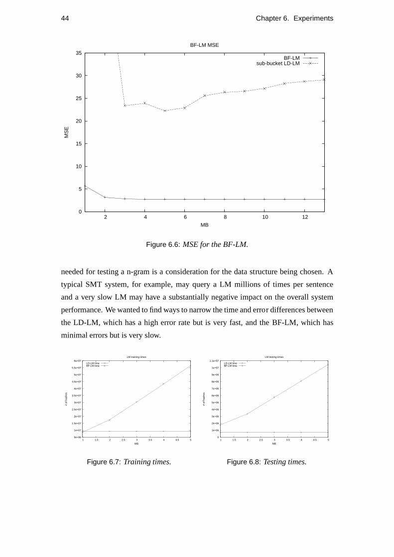
44 Chapter 6. Experiments
0
5
10
15
20
25
30
35
2 4 6 8 10 12
MS
E
MB
BF-LM MSE
BF-LMsub-bucket LD-LM
Figure 6.6: MSE for the BF-LM.
needed for testing a n-gram is a consideration for the data structure being chosen. A
typical SMT system, for example, may query a LM millions of times per sentence
and a very slow LM may have a substantially negative impact onthe overall system
performance. We wanted to find ways to narrow the time and error differences between
the LD-LM, which has a high error rate but is very fast, and theBF-LM, which has
minimal errors but is very slow.
5e+06
1e+07
1.5e+07
2e+07
2.5e+07
3e+07
3.5e+07
4e+07
4.5e+07
5e+07
5.5e+07
6e+07
1 1.5 2 2.5 3 3.5 4 4.5 5
# of
has
hes
MB
LM training times
LD-LM timeBF-LM time
Figure 6.7: Training times.
0
1e+06
2e+06
3e+06
4e+06
5e+06
6e+06
7e+06
8e+06
9e+06
1e+07
1.1e+07
1 1.5 2 2.5 3 3.5 4 4.5 5
# of
has
hes
MB
LM testing times
LD-LM timeBF-LM time
Figure 6.8: Testing times.

6.4. Composite LD-LM 45
6.4 Composite LD-LM
We implemented a new scheme for the LD-LM that encoded n-grams and their quan-
tized frequencies directly as composite events and, like the BF-LM, used runtime
smoothing during testing. The frequencies were quantized and expected counts re-
trieved with the same formulas used in the BF-LM. We smoothedwith Stupid Backoff.
We still kept exact sub-buckets for the n-gram signature andthe counts, but as we no
longer needed a sub-bucket for a backoff probability there was more bits available for
the n-gram signature. Also, because we know the highest frequency in our training
corpus we can explicitly set the number of bits of this sub-bucket to be what we need.
For example, using only 3 bits for the quantized counts wouldonly give us a maximum
of 749 for our retrieved expected count. However, using 4 bits gives a maximum of
over 6 million.
0
20
40
60
80
100
1 2 3 4 5 6 7 8 9 10
MS
E
MB
Composite LD-LM Error Rates
random 32-bitordered 32-bitrandom 16-bitordered 16-bit
random 8-bitordered 8-bit
Figure 6.9: The MSE for the unordered composite LD-LM for lower space bounds are
not comparable to that of the ordered LD-LM.
This scheme led to a lower false positive rate than the sub-bucket LD as we used
more space for the signature of each event and, as we no longerdiscarded probability
information for each event of the LM, a lower MSE too. The figure in 6.9 shows
the MSE for the different space parameters and bit models of the composite LD both.
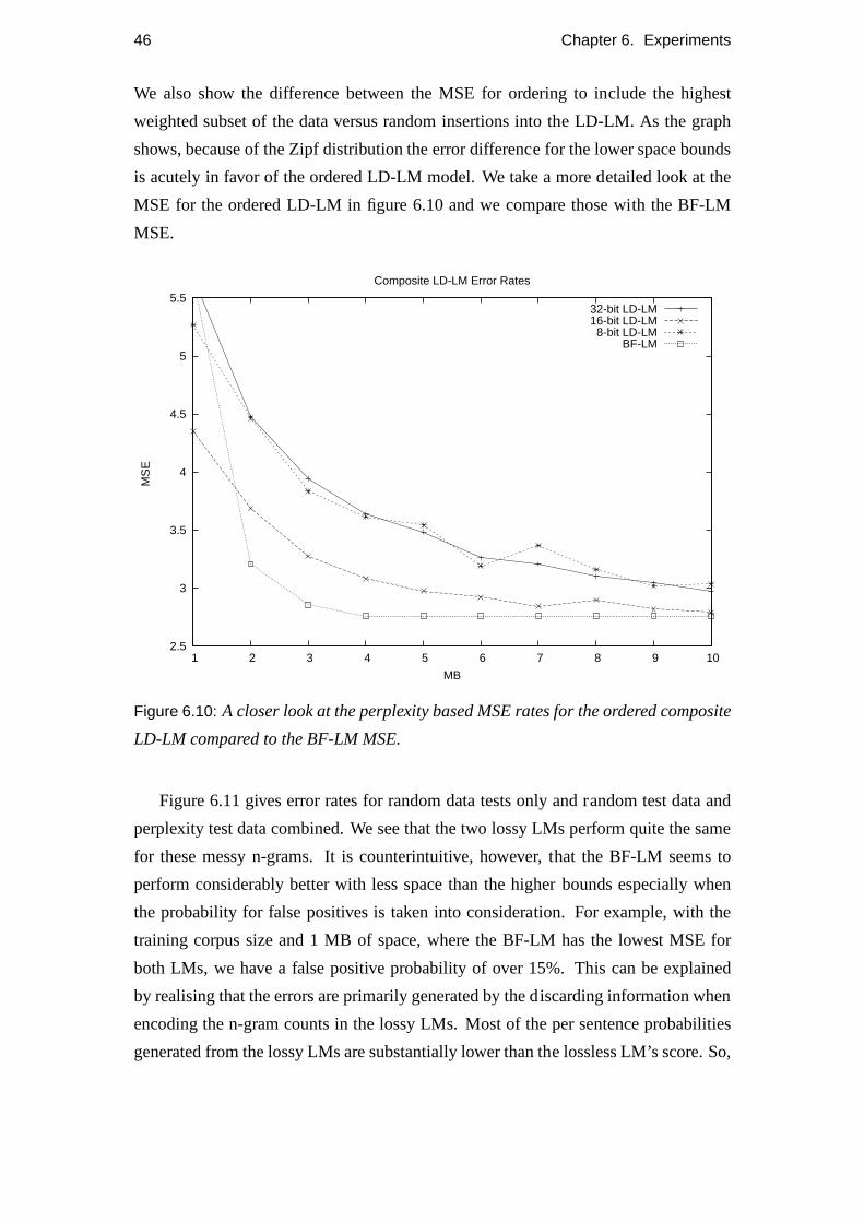
46 Chapter 6. Experiments
We also show the difference between the MSE for ordering to include the highest
weighted subset of the data versus random insertions into the LD-LM. As the graph
shows, because of the Zipf distribution the error difference for the lower space bounds
is acutely in favor of the ordered LD-LM model. We take a more detailed look at the
MSE for the ordered LD-LM in figure 6.10 and we compare those with the BF-LM
MSE.
2.5
3
3.5
4
4.5
5
5.5
1 2 3 4 5 6 7 8 9 10
MS
E
MB
Composite LD-LM Error Rates
32-bit LD-LM16-bit LD-LM8-bit LD-LM
BF-LM
Figure 6.10: A closer look at the perplexity based MSE rates for the ordered composite
LD-LM compared to the BF-LM MSE.
Figure 6.11 gives error rates for random data tests only and random test data and
perplexity test data combined. We see that the two lossy LMs perform quite the same
for these messy n-grams. It is counterintuitive, however, that the BF-LM seems to
perform considerably better with less space than the higherbounds especially when
the probability for false positives is taken into consideration. For example, with the
training corpus size and 1 MB of space, where the BF-LM has thelowest MSE for
both LMs, we have a false positive probability of over 15%. This can be explained
by realising that the errors are primarily generated by the discarding information when
encoding the n-gram counts in the lossy LMs. Most of the per sentence probabilities
generated from the lossy LMs are substantially lower than the lossless LM’s score. So,
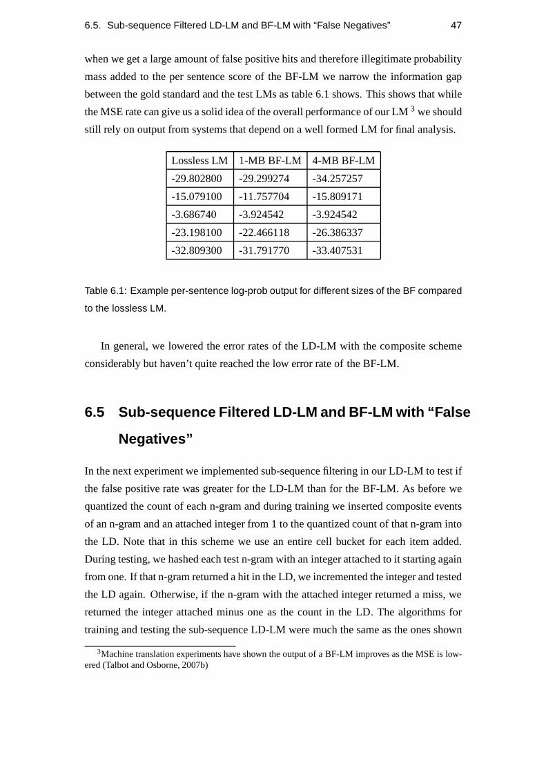
6.5. Sub-sequence Filtered LD-LM and BF-LM with “False Negatives” 47
when we get a large amount of false positive hits and therefore illegitimate probability
mass added to the per sentence score of the BF-LM we narrow theinformation gap
between the gold standard and the test LMs as table 6.1 shows.This shows that while
the MSE rate can give us a solid idea of the overall performance of our LM3 we should
still rely on output from systems that depend on a well formedLM for final analysis.
Lossless LM 1-MB BF-LM 4-MB BF-LM
-29.802800 -29.299274 -34.257257
-15.079100 -11.757704 -15.809171
-3.686740 -3.924542 -3.924542
-23.198100 -22.466118 -26.386337
-32.809300 -31.791770 -33.407531
Table 6.1: Example per-sentence log-prob output for different sizes of the BF compared
to the lossless LM.
In general, we lowered the error rates of the LD-LM with the composite scheme
considerably but haven’t quite reached the low error rate ofthe BF-LM.
6.5 Sub-sequence Filtered LD-LM and BF-LM with “False
Negatives”
In the next experiment we implemented sub-sequence filtering in our LD-LM to test if
the false positive rate was greater for the LD-LM than for theBF-LM. As before we
quantized the count of each n-gram and during training we inserted composite events
of an n-gram and an attached integer from 1 to the quantized count of that n-gram into
the LD. Note that in this scheme we use an entire cell bucket for each item added.
During testing, we hashed each test n-gram with an integer attached to it starting again
from one. If that n-gram returned a hit in the LD, we incremented the integer and tested
the LD again. Otherwise, if the n-gram with the attached integer returned a miss, we
returned the integer attached minus one as the count in the LD. The algorithms for
training and testing the sub-sequence LD-LM were much the same as the ones shown
3Machine translation experiments have shown the output of a BF-LM improves as the MSE is low-ered (Talbot and Osborne, 2007b)

48 Chapter 6. Experiments
15
16
17
18
19
20
21
22
23
0 2 4 6 8 10 12
MS
E
MB
Error Rates
rand-LDrand-BFmix-LD
mix-LDBF
Figure 6.11: When we test purely random data the MSE for the BF-LM and LD-LM
are nearly equivalent or in favor of the LD-LM. The lower BF-LM MSE for the lowest
space bounds are because of the extra probability mass from the false positives.
in figure 4.1 on Sect. 4 except for the data structure used. Thepseudocode for our
implementation is listed in Appendix A.
From the higher MSE numbers in graph 6.12 we can guess that it’s not the false
positives in the LD-LM that increase the error rates but the amount of false negatives
or information that is discarded from the set that negatively effect it. To verify this,
we trained the BF-LM with only the subset of n-gram events andtheir counts that
were entered into the LD-LM inducing the same false negativerate in both PDSs. As
expected, the graph in figure 6.13 the MSE between the two lossy LMs are basically
identical.
6.6 Bloom Dictionary LM
The reason the BF can maintain its one-sided error is becauseit shares the bit space
between events in the set it encodes. This is impossible to dowith a bucket scheme
such as the LD where each event gets a distinct allocation of bits only to itself. In this
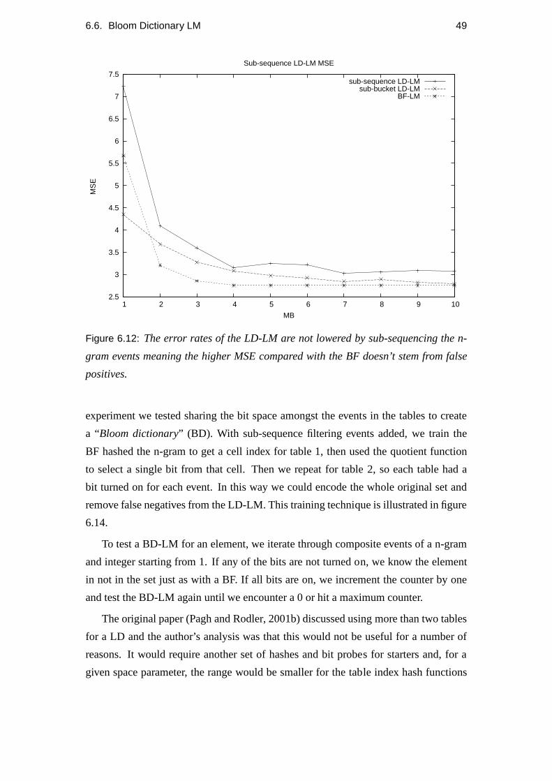
6.6. Bloom Dictionary LM 49
2.5
3
3.5
4
4.5
5
5.5
6
6.5
7
7.5
1 2 3 4 5 6 7 8 9 10
MS
E
MB
Sub-sequence LD-LM MSE
sub-sequence LD-LMsub-bucket LD-LM
BF-LM
Figure 6.12: The error rates of the LD-LM are not lowered by sub-sequencing the n-
gram events meaning the higher MSE compared with the BF doesn’t stem from false
positives.
experiment we tested sharing the bit space amongst the events in the tables to create
a “Bloom dictionary” (BD). With sub-sequence filtering events added, we train the
BF hashed the n-gram to get a cell index for table 1, then used the quotient function
to select a single bit from that cell. Then we repeat for table2, so each table had a
bit turned on for each event. In this way we could encode the whole original set and
remove false negatives from the LD-LM. This training technique is illustrated in figure
6.14.
To test a BD-LM for an element, we iterate through composite events of a n-gram
and integer starting from 1. If any of the bits are not turned on, we know the element
in not in the set just as with a BF. If all bits are on, we increment the counter by one
and test the BD-LM again until we encounter a 0 or hit a maximumcounter.
The original paper (Pagh and Rodler, 2001b) discussed usingmore than two tables
for a LD and the author’s analysis was that this would not be useful for a number of
reasons. It would require another set of hashes and bit probes for starters and, for a
given space parameter, the range would be smaller for the table index hash functions

50 Chapter 6. Experiments
2.6
2.8
3
3.2
3.4
3.6
3.8
4
4.2
4.4
4.6
4.8
1 2 3 4 5 6 7 8 9 10
MS
E
MB
BF-LM with "false negatives" MSE
LD-LMBF-LM
Figure 6.13: Using the same subset of n-grams included in the LD-LM for theBF-LM
(so the BF-LM imitates the false negatives of the LD-LM) results in nearly identical
MSE between the two PDSs.
so the quotient bits in each cell may need more space to reducefalse positives. Also,
it would increase the uncertainty of which table the data should be inserted into and
retrieved from. For our purposes, however, executing another pair of hashes would still
keep the LD-LM time constant which would still be a marked improvement over the
BF-LM times. Further, with bit sharing it doesn’t matter about the reduced index range
of each table since now we use every table for each n-gram which also means there is
no level of uncertainty about which table to use. So we testedusing more than two
tables as well with positive results as the graph in figure 6.15 shows. Also, because
we’re now only setting a bit a cell, we used only 8-bts per cellto increase the range of
each table for the space bound set.
6.6.1 BD Properties
Encoding the whole set lowers the error to at least that of theBF-LD, so we have
achieved a PDS encoded LM with constant time and low error rates. However, a closer
look at the properties of the BD shows of course it’s only a basic variant of a BF. From
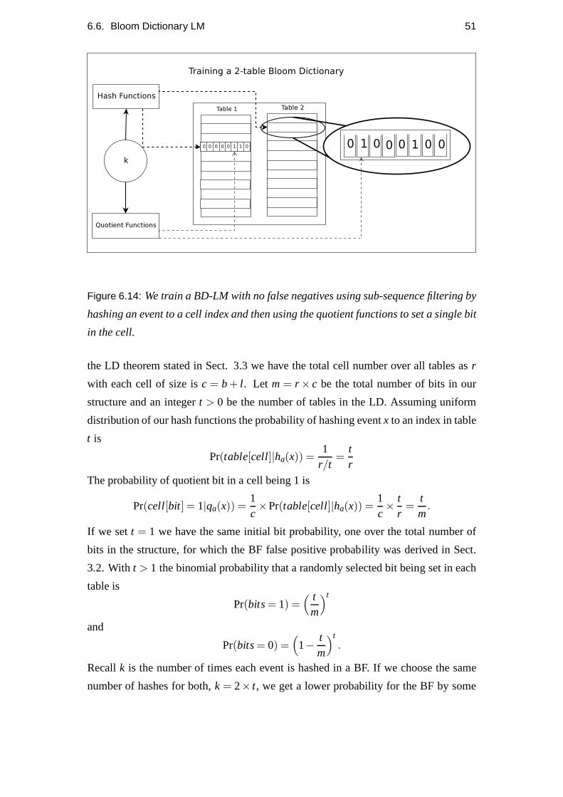
6.6. Bloom Dictionary LM 51
Figure 6.14: We train a BD-LM with no false negatives using sub-sequence filtering by
hashing an event to a cell index and then using the quotient functions to set a single bit
in the cell.
the LD theorem stated in Sect. 3.3 we have the total cell number over all tables asr
with each cell of size isc = b+ l . Let m = r × c be the total number of bits in our
structure and an integert > 0 be the number of tables in the LD. Assuming uniform
distribution of our hash functions the probability of hashing eventx to an index in table
t is
Pr(table[cell]|ha(x)) =1
r/t=
tr
The probability of quotient bit in a cell being 1 is
Pr(cell[bit] = 1|qa(x)) =1c×Pr(table[cell]|ha(x)) =
1c×
tr
=tm
.
If we sett = 1 we have the same initial bit probability, one over the totalnumber of
bits in the structure, for which the BF false positive probability was derived in Sect.
3.2. Witht > 1 the binomial probability that a randomly selected bit being set in each
table is
Pr(bits= 1) =( t
m
)t
and
Pr(bits= 0) =(
1−tm
)t.
Recallk is the number of times each event is hashed in a BF. If we choosethe same
number of hashes for both,k = 2× t, we get a lower probability for the BF by some
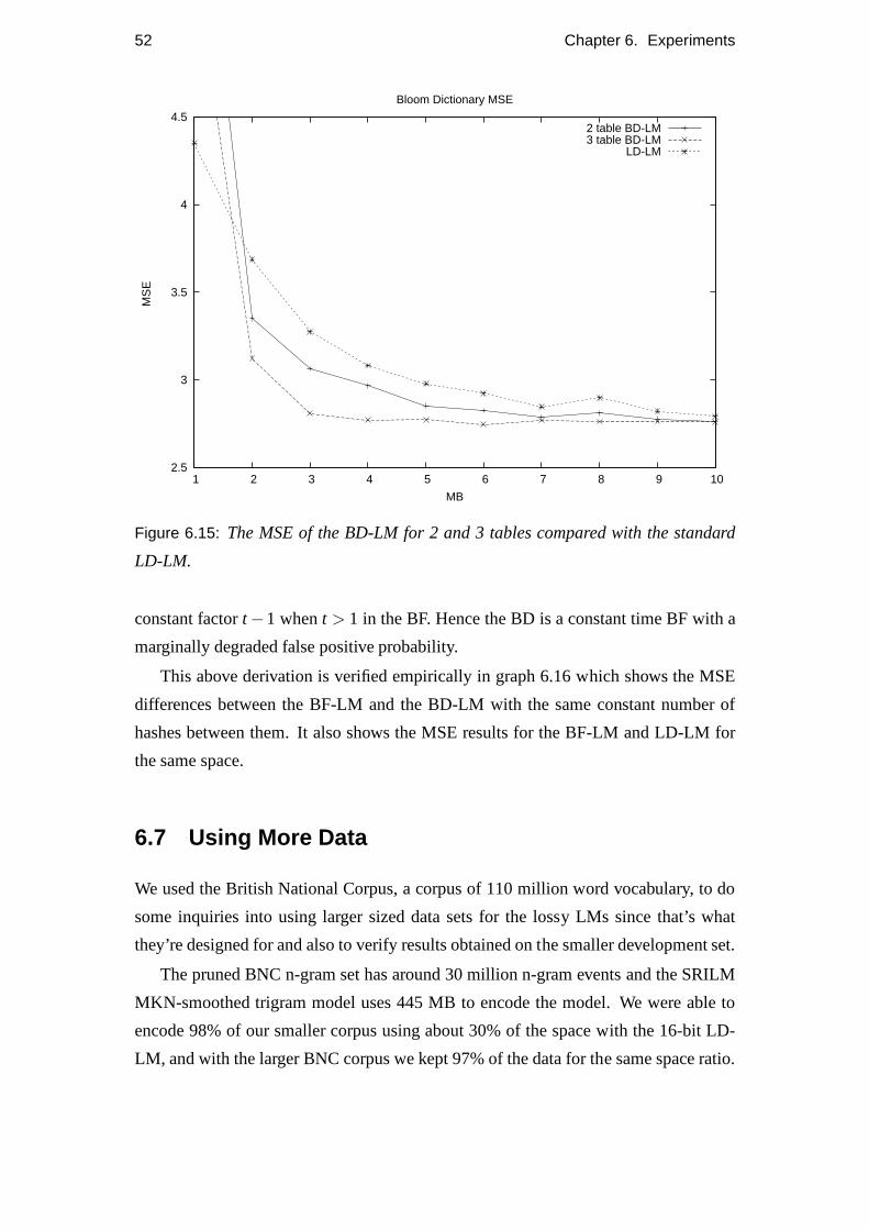
52 Chapter 6. Experiments
2.5
3
3.5
4
4.5
1 2 3 4 5 6 7 8 9 10
MS
E
MB
Bloom Dictionary MSE
2 table BD-LM3 table BD-LM
LD-LM
Figure 6.15: The MSE of the BD-LM for 2 and 3 tables compared with the standard
LD-LM.
constant factort −1 whent > 1 in the BF. Hence the BD is a constant time BF with a
marginally degraded false positive probability.
This above derivation is verified empirically in graph 6.16 which shows the MSE
differences between the BF-LM and the BD-LM with the same constant number of
hashes between them. It also shows the MSE results for the BF-LM and LD-LM for
the same space.
6.7 Using More Data
We used the British National Corpus, a corpus of 110 million word vocabulary, to do
some inquiries into using larger sized data sets for the lossy LMs since that’s what
they’re designed for and also to verify results obtained on the smaller development set.
The pruned BNC n-gram set has around 30 million n-gram eventsand the SRILM
MKN-smoothed trigram model uses 445 MB to encode the model. We were able to
encode 98% of our smaller corpus using about 30% of the space with the 16-bit LD-
LM, and with the larger BNC corpus we kept 97% of the data for the same space ratio.
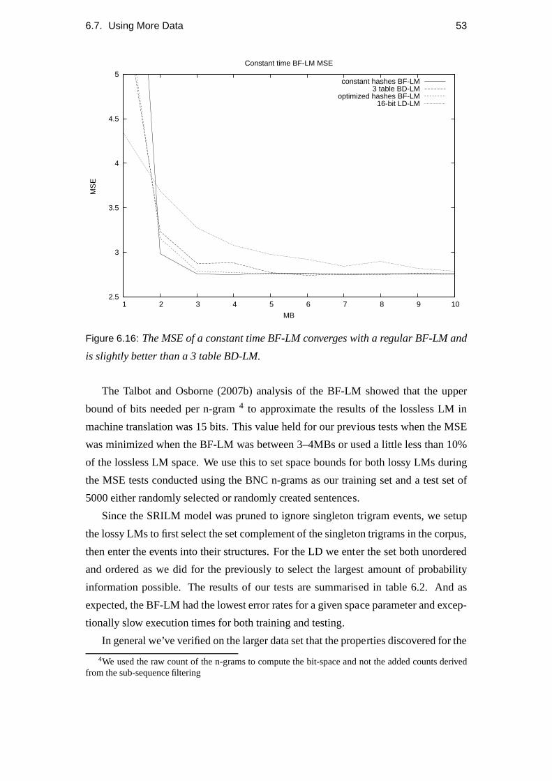
6.7. Using More Data 53
2.5
3
3.5
4
4.5
5
1 2 3 4 5 6 7 8 9 10
MS
E
MB
Constant time BF-LM MSE
constant hashes BF-LM3 table BD-LM
optimized hashes BF-LM16-bit LD-LM
Figure 6.16: The MSE of a constant time BF-LM converges with a regular BF-LM and
is slightly better than a 3 table BD-LM.
The Talbot and Osborne (2007b) analysis of the BF-LM showed that the upper
bound of bits needed per n-gram4 to approximate the results of the lossless LM in
machine translation was 15 bits. This value held for our previous tests when the MSE
was minimized when the BF-LM was between 3–4MBs or used a little less than 10%
of the lossless LM space. We use this to set space bounds for both lossy LMs during
the MSE tests conducted using the BNC n-grams as our trainingset and a test set of
5000 either randomly selected or randomly created sentences.
Since the SRILM model was pruned to ignore singleton trigramevents, we setup
the lossy LMs to first select the set complement of the singleton trigrams in the corpus,
then enter the events into their structures. For the LD we enter the set both unordered
and ordered as we did for the previously to select the largestamount of probability
information possible. The results of our tests are summarised in table 6.2. And as
expected, the BF-LM had the lowest error rates for a given space parameter and excep-
tionally slow execution times for both training and testing.
In general we’ve verified on the larger data set that the properties discovered for the
4We used the raw count of the n-grams to compute the bit-space and not the added counts derivedfrom the sub-sequence filtering

54 Chapter 6. Experiments
Table 6.2: Training and Testing with the BNC Corpus
LM Type Size MSE % data kept
Lossless LM 445MB N/A 100
BF-LM 50 3.669 100
Unsorted LD-LM 50 17.66 76.30
Sorted LD-LM 50 5.25 76.80
Sorted LD-LM 133 2.73 97.6
BD-LM 50 4.416 100
lossy LMs using the smaller training set hold over scale. This is important as Google’s
Trillion Word N-gram set, for example, is exponentially larger than data sets we’ve
been working with.

Chapter 7
Conclusions and Further Work
We’ve reimplemented the lossy BF-LM work of Talbot and Osborne (2007a) and com-
pared its properties with the first implementation using a LDas the encoding data
structure for a LM. Much of the research time was spent tryingand testing various
ways to best represent the n-grams in the LD space. Also, as Lossy LMs are a new
area of investigation in NLP, this is the first comparison between two PDSs suited for
their use.
Our findings follow directly with the properties of these data structures. With equal
space bounds between them the BF-LM’s one-sided error ratesare lower than the LD-
LM’s two-sided error. Without the ability to enter the wholen-gram set we can’t get
rid of false negatives so we can’t bridge the difference in the error rates between the
BF-LM and the LD-LM. Because of the bit-sharing, the BF-LM also has a significant
space advantage over the LD which requires an exclusive bit-bucket per event in then
n-gram set. The LD-LM relies on including the highest valuedsubset of the data to
keep it’s error rates low. The LD-LM is many times faster thenthe BF-LM and, with
its native support of associated information with key/value pairs, simple to setup as a
smoothed LM since there is no need for sub-sequence filtering. We also found with
sub-sequence filtering we can combine the constant access time of the LD and the bit
sharing of the BF to create a bit-sharing LM that is fast, represents the whole set of
n-grams, and returns minimal errors.
Unfortunately time constraints did not enable us to do all the experiments we would
have liked for this report. As we mainly concentrated on the properties of the lossy
LMs in the abstract there is still more work to do testing the LD-LM in a real-world
application such as an SMT system. In general this work should not be considered
complete until this is done especially as our experiments showed that the MSE doesn’t
55
56 Chapter 7. Conclusions and Further Work
tell the entire story regarding the overall goodness of a lossy LM. The only previous
work of this type, reported in Talbot and Osborne (2007b), tested the BF-LM in a
SMT system where translation with the lossy BF-LM matched the BLEU scores of
translations that used a lossless LM but it also took between2 and 5 times longer
for each translation experiment. It would be interesting todiscover for what space
bounds the LD-LM can match these same BLEU scores. This wouldalso show what
ratio of data in the huge n-gram sets is actually made use of for these tasks. It would
also be interesting to see how the BD-LM performs in an application environment. If
the results of this research hold, we should be able to match the BLEU scores of a
lossless LM without extending translation time at all and still maintain a significant
space advantage overall.
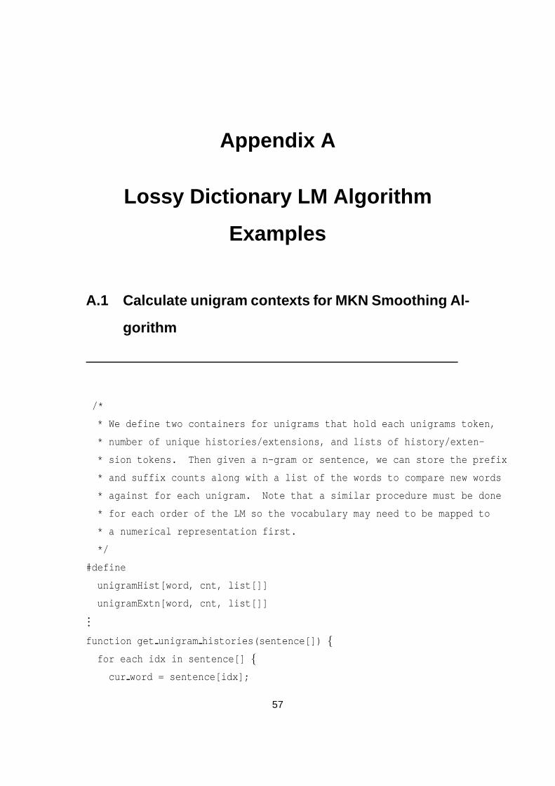
Appendix A
Lossy Dictionary LM Algorithm
Examples
A.1 Calculate unigram contexts for MKN Smoothing Al-
gorithm
/*
* We define two containers for unigrams that hold each unigra ms token,
* number of unique histories/extensions, and lists of histo ry/exten-
* sion tokens. Then given a n-gram or sentence, we can store th e prefix
* and suffix counts along with a list of the words to compare ne w words
* against for each unigram. Note that a similar procedure mus t be done
* for each order of the LM so the vocabulary may need to be mappe d to
* a numerical representation first.
*/
#define
unigramHist[word, cnt, list[]]
unigramExtn[word, cnt, list[]]...
function get unigram histories(sentence[]) {
for each idx in sentence[] {
cur word = sentence[idx];
57

58 Appendix A. Lossy Dictionary LM Algorithm Examples
prev word = sentence[idx - 1];
next word = sentence[idx + 1];
if(cur word in unigramHist[]) {
if(prev word not in unigramHist[cur word].list[]) {
add prev word to unigramHist[cur word].list[];
/* increment count of histories for unigram */
unigramHist[cur word].cnt ++;
}
}
else {
add cur word to unigramHist[];
add prev word to unigramHist[cur word].list[];
/* new history so set history counter to 1 */
unigramHist[cur word].cnt = 1;
}
if(cur word in unigramExtn[]) {
if(next word not in unigramExtn[cur word].list[]) {
add next word to unigramExtn[cur word].list[];
/* increment unique extension counter */
unigramExtn[cur word].cnt ++;
}
}
else {
add cur word to unigramExtn[];
add next word to unigramExtn[cur word].list[];
unigramExtn[cur word].cnt = 1;
}
}
}
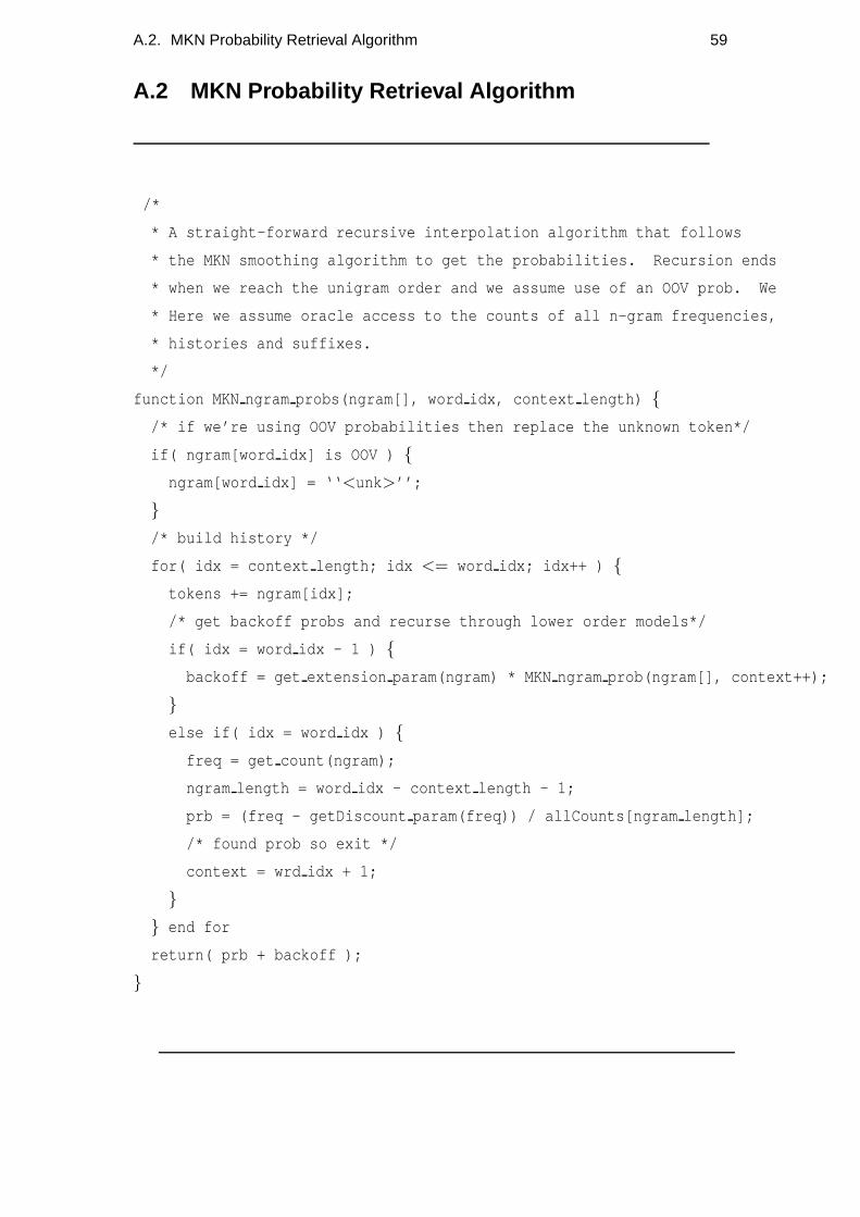
A.2. MKN Probability Retrieval Algorithm 59
A.2 MKN Probability Retrieval Algorithm
/*
* A straight-forward recursive interpolation algorithm th at follows
* the MKN smoothing algorithm to get the probabilities. Recu rsion ends
* when we reach the unigram order and we assume use of an OOV pro b. We
* Here we assume oracle access to the counts of all n-gram freq uencies,
* histories and suffixes.
*/
function MKN ngram probs(ngram[], word idx, context length) {
/* if we’re using OOV probabilities then replace the unknown token*/
if( ngram[word idx] is OOV ) {
ngram[word idx] = ‘‘ <unk >’’;
}
/* build history */
for( idx = context length; idx <= word idx; idx++ ) {
tokens += ngram[idx];
/* get backoff probs and recurse through lower order models* /
if( idx = word idx - 1 ) {
backoff = get extension param(ngram) * MKN ngram prob(ngram[], context++);
}
else if( idx = word idx ) {
freq = get count(ngram);
ngram length = word idx - context length - 1;
prb = (freq - getDiscount param(freq)) / allCounts[ngram length];
/* found prob so exit */
context = wrd idx + 1;
}
} end for
return( prb + backoff );
}

60 Appendix A. Lossy Dictionary LM Algorithm Examples
A.3 Sub-bucket LD-LM training and testing algorithms
/* Our sub-bucket LD-LM training and testing algorithms use d a series
* of bit-shifts and bit-masks to place and retrieve values in a bit-
* bucket. The << and >> are left and right bit-shift operators
* and & is the bitwise AND operator.
*/
#define
/* sub-bucket sizes and bit-masks */
NGRAMBITS 8
PRB BITS 4
BKOFFBITS 4
QUOTMASK (2NGRAM BITS - 1) << (PROB BITS + BKOFF BITS)
PRB MASK (2PRB BITS - 1) << BKOFFBITS
BKOFFMASK 2BKOFF BITS - 1...
function train(ngram, prb, bkoff) {
/* create composite value of [signature + prob + backoff] */
cell value = get quotient signature(ngram) << (PRB BITS + BKOFF BITS);
cell value = cell value + (quantize(prb, d = 1) << BKOFFBITS);
cell value = cell value + quantize(bkoff, d = 3);
/* get table 1 index and insert if empty */
idx = hash 1(ngram) mod table size;
if( table 1[idx] is empty ) {
table 1[idx] = cell value;
}
else {
/* get table 2 index and insert if empty */
idx = hash 2(ngram) mod table size;
if( table 2[idx] is empty ) {
table 2[idx] = cell value;
}
else {
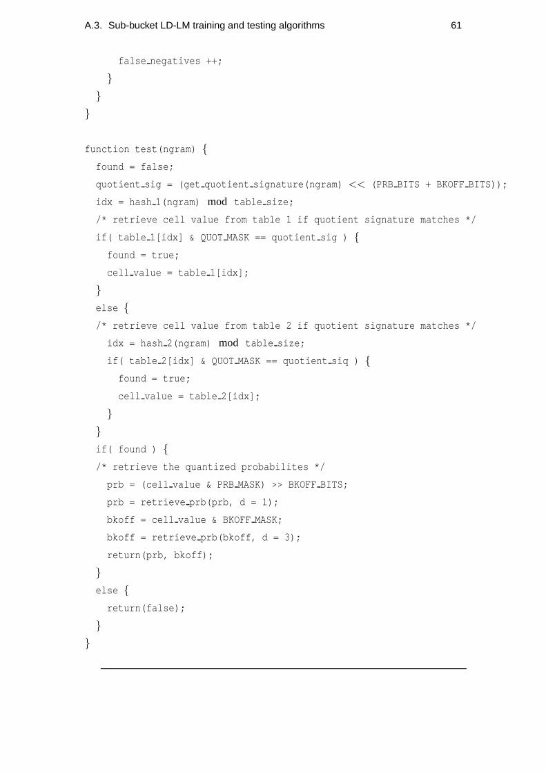
A.3. Sub-bucket LD-LM training and testing algorithms 61
false negatives ++;
}
}
}
function test(ngram) {
found = false;
quotient sig = (get quotient signature(ngram) << (PRB BITS + BKOFF BITS));
idx = hash 1(ngram) mod table size;
/* retrieve cell value from table 1 if quotient signature mat ches */
if( table 1[idx] & QUOT MASK == quotient sig ) {
found = true;
cell value = table 1[idx];
}
else {
/* retrieve cell value from table 2 if quotient signature mat ches */
idx = hash 2(ngram) mod table size;
if( table 2[idx] & QUOT MASK == quotient siq ) {
found = true;
cell value = table 2[idx];
}
}
if( found ) {
/* retrieve the quantized probabilites */
prb = (cell value & PRB MASK) >> BKOFFBITS;
prb = retrieve prb(prb, d = 1);
bkoff = cell value & BKOFF MASK;
bkoff = retrieve prb(bkoff, d = 3);
return(prb, bkoff);
}
else {
return(false);
}
}
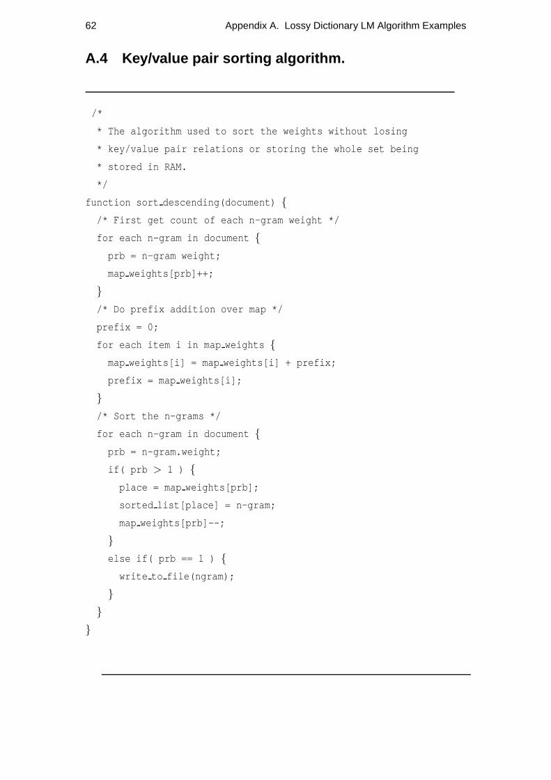
62 Appendix A. Lossy Dictionary LM Algorithm Examples
A.4 Key/value pair sorting algorithm.
/*
* The algorithm used to sort the weights without losing
* key/value pair relations or storing the whole set being
* stored in RAM.
*/
function sort descending(document) {
/* First get count of each n-gram weight */
for each n-gram in document {
prb = n-gram weight;
map weights[prb]++;
}
/* Do prefix addition over map */
prefix = 0;
for each item i in map weights {
map weights[i] = map weights[i] + prefix;
prefix = map weights[i];
}
/* Sort the n-grams */
for each n-gram in document {
prb = n-gram.weight;
if( prb > 1 ) {
place = map weights[prb];
sorted list[place] = n-gram;
map weights[prb]--;
}
else if( prb == 1 ) {
write to file(ngram);
}
}
}
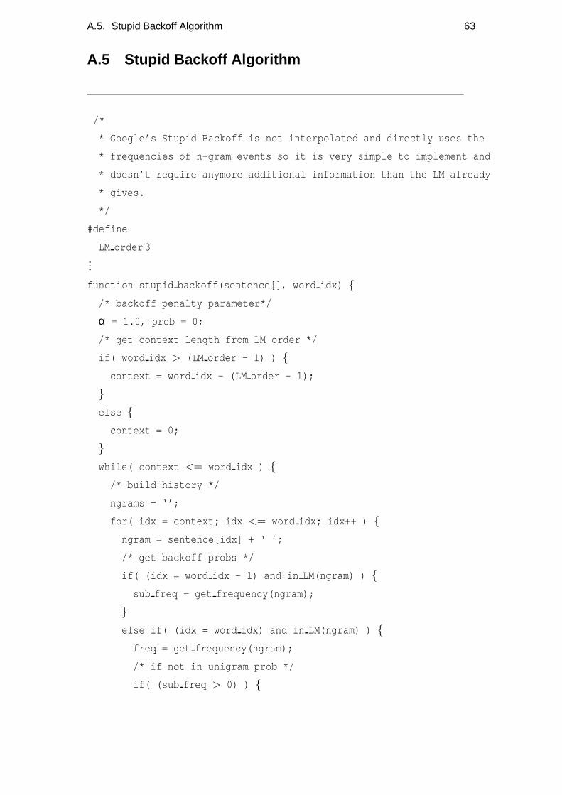
A.5. Stupid Backoff Algorithm 63
A.5 Stupid Backoff Algorithm
/*
* Google’s Stupid Backoff is not interpolated and directly u ses the
* frequencies of n-gram events so it is very simple to impleme nt and
* doesn’t require anymore additional information than the L M already
* gives.
*/
#define
LM order 3...
function stupid backoff(sentence[], word idx) {
/* backoff penalty parameter*/
α = 1.0, prob = 0;
/* get context length from LM order */
if( word idx > (LM order - 1) ) {
context = word idx - (LM order - 1);
}
else {
context = 0;
}
while( context <= word idx ) {
/* build history */
ngrams = ‘’;
for( idx = context; idx <= word idx; idx++ ) {
ngram = sentence[idx] + ‘ ’;
/* get backoff probs */
if( (idx = word idx - 1) and in LM(ngram) ) {
sub freq = get frequency(ngram);
}
else if( (idx = word idx) and in LM(ngram) ) {
freq = get frequency(ngram);
/* if not in unigram prob */
if( (sub freq > 0) ) {
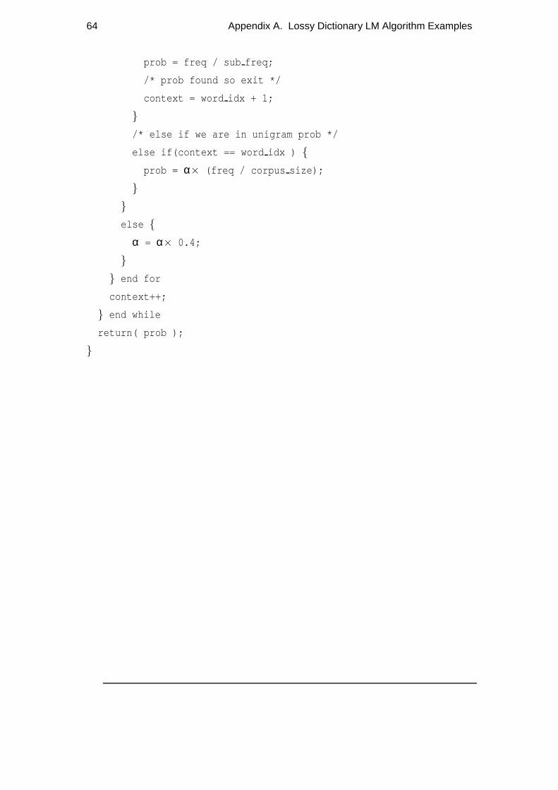
64 Appendix A. Lossy Dictionary LM Algorithm Examples
prob = freq / sub freq;
/* prob found so exit */
context = word idx + 1;
}
/* else if we are in unigram prob */
else if(context == word idx ) {
prob = α× (freq / corpus size);
}
}
else {
α = α× 0.4;
}
} end for
context++;
} end while
return( prob );
}
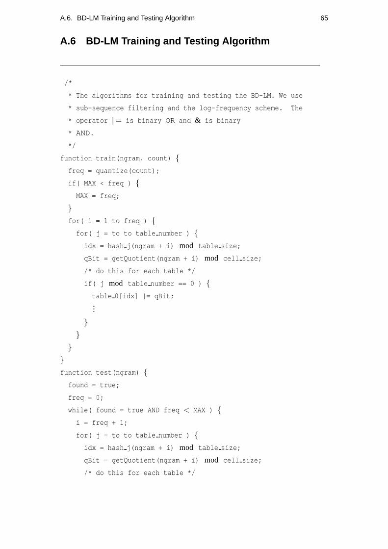
A.6. BD-LM Training and Testing Algorithm 65
A.6 BD-LM Training and Testing Algorithm
/*
* The algorithms for training and testing the BD-LM. We use
* sub-sequence filtering and the log-frequency scheme. The
* operator | = is binary OR and & is binary
* AND.
*/
function train(ngram, count) {
freq = quantize(count);
if( MAX < freq ) {
MAX = freq;
}
for( i = 1 to freq ) {
for( j = to to table number ) {
idx = hash j(ngram + i) mod table size;
qBit = getQuotient(ngram + i) mod cell size;
/* do this for each table */
if( j mod table number == 0 ) {
table 0[idx] |= qBit;...
}
}
}
}
function test(ngram) {
found = true;
freq = 0;
while( found = true AND freq < MAX ) {
i = freq + 1;
for( j = to to table number ) {
idx = hash j(ngram + i) mod table size;
qBit = getQuotient(ngram + i) mod cell size;
/* do this for each table */
66 Appendix A. Lossy Dictionary LM Algorithm Examples
if( j mod table number == 0 ) {
if( (table 0[idx] & qBit) not equal qBit ) {
found = false;...
}
}
}
}
if( freq > 0 ) {
freq = retrieveExpectedCount(freq);
}
return( freq );
}

Bibliography
Algoet, P. H. and Cover, T. M. (1988). A sandwich proof of the shannon-mcmillan-breiman theorem.The Annals of Probability, 16(2):899–909.
Bloom, B. H. (1970). Space/time trade-offs in hash coding with allowable errors.Commun. ACM, 13(7):422–426.
Brants, T., Popat, A. C., Xu, P., Och, F. J., and Dean, J. (2007). Large language modelsin machine translation. InProceedings of the 2007 Joint Conference on EmpiricalMethods in Natural Language Processing and Computational Natural LanguageLearning (EMNLP-CoNLL), pages 858–867.
Broder, A. and Mitzenmacher, M. (2002). Network applications of bloom filters: Asurvey. InIn Proc. of Allerton Conference.
Brown, P. F., Pietra, V. J. D., Mercer, R. L., Pietra, S. A. D.,and Lai, J. C. (1992). Anestimate of an upper bound for the entropy of english.Comput. Linguist., 18(1):31–40.
Carter, J. L. and Wegman, M. N. (1977). Universal classes of hash functions (extendedabstract). InSTOC ’77: Proceedings of the ninth annual ACM symposium on Theoryof computing, pages 106–112, New York, NY, USA. ACM Press.
Chazelle, B., Kilian, J., Rubinfeld, R., and Tal, A. (2004).The bloomier filter: anefficient data structure for static support lookup tables. In SODA ’04: Proceedingsof the fifteenth annual ACM-SIAM symposium on Discrete algorithms, pages 30–39,Philadelphia, PA, USA. Society for Industrial and Applied Mathematics.
Chen, S. and Goodman, J. (October 1999). An empirical study of smoothing tech-niques for language modeling.Computer Speech & Language, 13:359–393(35).
Cormen, T. H., Leiserson, C. E., Rivest, R. L., and Stein, C. (2001). Introduction toAlgorithms. The MIT Press, 2nd edition.
Costa, L. H. M. K., Fdida, S., and Duarte, O. C. M. B. (2006). Incremental servicedeployment using the hop-by-hop multicast routing protocol. IEEE/ACM Trans.Netw., 14(3):543–556.
Cover, T. and King, R. (1978). A convergent gambling estimate of the entropy ofEnglish. IEEE Transactions of Information Theory, IT-24:413–421.
67
68 Bibliography
Cover, T. and Thomas, J. (1990).Elements of Information Theory. John Wiley, NewYork.
de Boer, P.-T., Droese, D., Mannor, S., and Rubinstein, R. (February 2005). A tutorialon the cross-entropy method.Annals of Operations Research, 134:19–67(49).
de Laplace, M. (1996).A Philosophical Essay on Probabilities. Dover Publications.
Fan, L., Cao, P., Almeida, J., and Broder, A. Z. (2000). Summary cache: a scalablewide-area Web cache sharing protocol.IEEE/ACM Transactions on Networking,8(3):281–293.
Hagerup, T. (1998). Sorting and searching on the word ram. InSTACS ’98: Proceed-ings of the 15th Annual Symposium on Theoretical Aspects of Computer Science,pages 366–398, London, UK. Springer-Verlag.
Hurd, J. (2003). Formal verification of probabilistic algorithms. Technical Report 566,University of Cambridge Computer Laboratory.
James, F. (2000). Modified kneser-ney smoothing of n-gram models. Technical report,Research Institute for Advanced Computer Science.
Jurafsky, D. and Martin, J. H. (2000).Speech and Language Processing. An Intro-duction to Natural Language Processsing, Computational Linguistics, and SpeechRecognition.Prentice Hall. New Jersey.
Kneser, R. and Ney, H. (1995). Improved backing-off for m-gram language modelling.In Proceedings of the IEEE Conference on Acoustics, Speech andSignal Processing,volume 1, pages 181–184.
Koehn, P. (2003). Europarl: A multilingual cor-pus for evaluation of machine translation. Available athttp://people.csail.mit.edu/˜koehn/publications/eur oparl.ps .
Koehn, P. (2007). Empirical Methods in Natural Language Processing. from courseslides athttp://www.inf.ed.ac.uk/teaching/courses/emnlp/ .
Koehn, P. and Hoang, H. (2007). Factored translation models. In Proceedings of the2007 Joint Conference on Empirical Methods in Natural Language Processing andComputational Natural Language Learning (EMNLP-CoNLL), pages 868–876.
Koehn, P., Och, F. J., and Marcu, D. (2003). Statistical phrase-based translation. InNAACL ’03: Proceedings of the 2003 Conference of the North American Chapterof the Association for Computational Linguistics on Human Language Technology,pages 48–54, Morristown, NJ, USA. Association for Computational Linguistics.
Manning, C. D. and Schutze, H. (1999).Foundations of Statistical Natural LanguageProcessing. The M.I.T. Press. Massachusetts.
Mulvey, B. (2006). Hash functions.http://bretm.home.comcast.net/hash/ .

Bibliography 69
Norvig, P. (2007). Theorizing from data: Avoiding the capital mistake. Available athttp://www.youtube.com/watch?v=nU8DcBF-qo4 .
Och, F. (2005). The google statistical machine translationsystem for the 2005 nist mtevaluation, oral preesntation at the 2005 nist mt evaluation workshop.
Och, F. J. and Ney, H. (2001). Discriminative training and maximum entropy modelsfor statistical machine translation. InACL ’02: Proceedings of the 40th AnnualMeeting on Association for Computational Linguistics, pages 295–302, Morristown,NJ, USA. Association for Computational Linguistics.
Pagh, A., Pagh, R., and Rao, S. S. (2005). An optimal bloom filter replacement. InSODA ’05: Proceedings of the sixteenth annual ACM-SIAM symposium on Discretealgorithms, pages 823–829, Philadelphia, PA, USA. Society for Industrial and Ap-plied Mathematics.
Pagh, R. and Rodler, F. F. (2001a). Cuckoo hashing.Lecture Notes in ComputerScience, 2161:121–129.
Pagh, R. and Rodler, F. F. (2001b). Lossy dictionaries. InESA ’01: Proceedings ofthe 9th Annual European Symposium on Algorithms, pages 300–311, London, UK.Springer-Verlag.
Ravichandran, D., Pantel, P., and Hovy, E. (2005). Randomized algorithms and nlp:using locality sensitive hash function for high speed noun clustering. InACL ’05:Proceedings of the 43rd Annual Meeting on Association for Computational Linguis-tics, pages 622–629, Morristown, NJ, USA. Association for Computational Linguis-tics.
Shannon, C. (1951). Prediction and entropy of printed English.Bell Sys. Tech. Journal,30:50–64.
Stolcke, A. (2002). Srilm – an extensible language modelingtoolkit. In Proc. Intl.Conf. on Spoken Language Processing, 2002.
Talbot, D. and Osborne, M. (2007a). Randomised language modelling for statisticalmachine translation. InProceedings of the 45th Annual Meeting of the Associationof Computational Linguistics, pages 512–519, Prague, Czech Republic. Associationfor Computational Linguistics.
Talbot, D. and Osborne, M. (2007b). Smoothed Bloom filter language models: Tera-scale LMs on the cheap. InProceedings of the 2007 Joint Conference on EmpiricalMethods in Natural Language Processing and Computational Natural LanguageLearning (EMNLP-CoNLL), pages 468–476.