Embed Size (px)
Citation preview
Blocking Analysis of Spin Locks under
Partitioned Fixed-Priority Scheduling
Alexander Wieder
A dissertation submitted towards the degree
Doctor of natural sciences (Dr. rer. nat.)
of the faculty of mathematics and computer science
of Saarland University
Saarbrucken
January 2017

Colloquium
Date: 29.11.2017
Place: Saarbrucken
Dean: Prof. Dr. Frank-Olaf Schreyer
Examination Board
Chair: Prof. Dr. Sebastian Hack
Supervisor and Reviewer: Dr. Bjorn Brandenburg
Reviewer: Prof. Dr. Rupak Majumdar
Reviewer: Prof. Dr. Jan Reineke
Reviewer: Prof. Dr. Jian-Jia Chen
Scientific Assistant: Dr. Martin Zimmermann
© 2017
Alexander Wieder
ALL RIGHTS RESERVED
1
Abstract
Partitioned fixed-priority scheduling is widely used in embedded multicore
real-time systems. In multicore systems, spin locks are one well-known
technique used to synchronize conflicting accesses from different processor
cores to shared resources (e.g., data structures). The use of spin locks can
cause blocking. Accounting for blocking is a crucial part of static analysis
techniques to establish correct temporal behavior.
In this thesis, we consider two aspects inherent to the partitioned fixed-
priority scheduling of tasks sharing resources protected by spin locks: (1) the
assignment of tasks to processor cores to ensure correct timing, and (2) the
blocking analysis required to derive bounds on the blocking.
Heuristics commonly used for task assignment fail to produce assignments
that ensure correct timing when shared resources protected by spin locks
are used. We present an optimal approach that is guaranteed to find such
an assignment if it exists (under the original MSRP analysis). Further, we
present a well-performing and inexpensive heuristic.
For most spin lock types, no blocking analysis is available in prior work,
which renders them unusable in real-time systems. We present a blocking
analysis approach that supports eight different types and is less pessimistic
than prior analyses, where available. Further, we show that allowing nested
requests for FIFO- and priority-ordered locks renders the blocking analysis
problem NP -hard.
2

Zusammenfassung
Partitioned Fixed-Priority Scheduling ist in eingebetteten Multicore-Echtzeit-
systemen weit verbreitet. In Multicore-Systemen sind Spinlocks ein bekannter
Mechanismus um konkurrierende Zugriffe von unterschiedlichen Prozessork-
ernen auf geteilte Resourcen (z.B. Datenstrukturen) zu koordinieren. Bei der
Nutzung von Spinlocks konnen Blockierungen auftreten, die in statischen
Analysetechniken zum Nachweis des korrekten zeitlichen Verhaltens eines
Systems zu berucksichtigen sind.
Wir betrachten zwei Aspekte von Partitioned Fixed-Priority Scheduling in
Verbindung mit Spinlocks zum Schutz geteilter Resourcen: (1) die Zuweisung
von Tasks zu Prozessorkernen unter Einhaltung zeitlicher Vorgaben und
(2) die Analyse zur Entwicklung oberer Schranken fur die Blockierungs-
dauer.
Ubliche Heuristiken finden bei der Nutzung von Spinlocks oft keine Task-
zuweisung, bei der die Einhaltung zeitlicher Vorgaben garantiert ist. Wir
stellen einen optimalen Ansatz vor, der dies (mit der ursprunglichen MSRP
Analyse) garantiert, falls eine solche Zuweisung existiert. Zudem prasentieren
wir eine leistungsfahige Heuristik.
Die meisten Arten von Spinlocks konnen mangels Analyse der Blockierungs-
dauer nicht fur Echtzeitsysteme verwendet werden. Wir stellen einen Analy-
seansatz vor, der acht Spinlockarten unterstutzt und weniger pessimistische
Schranken liefert als vorherige Analysen, soweit vorhanden. Weiterhin zeigen
wir, dass die Analyse bei verschachtelten Zugriffen mit FIFO- und prioritats-
geordneten Locks ein NP -hartes Problem ist.
3

To my brother,
Maximilian Florian Wieder.
I tell you: one must still have chaos in oneself
to give birth to a dancing star.
I tell you: you still have chaos in yourselves.
—Friedrich Nietzsche, Thus Spoke Zarathustra
4

Meinem Bruder,
Maximilian Florian Wieder.
Ich sage euch: man muss noch Chaos in sich haben,
um einen tanzenden Stern gebaren zu konnen.
Ich sage euch: ihr habt noch Chaos in euch.
—Friedrich Nietzsche, Also sprach Zarathustra
5

Contents
1 Introduction 11
1.1 The Blocking Analysis Problem . . . . . . . . . . . . . . . . . 12
1.2 The Partitioning Problem . . . . . . . . . . . . . . . . . . . . 14
1.3 Scope of this Thesis . . . . . . . . . . . . . . . . . . . . . . . 15
1.4 Contributions . . . . . . . . . . . . . . . . . . . . . . . . . . . 16
1.4.1 Partitioning for Task Sets using Non-Nested Spin Locks 16
1.4.2 Blocking Analysis for Non-Nested Spin Locks . . . . . 17
1.4.3 Computational Complexity of Blocking Analysis for
Nested Spin Locks . . . . . . . . . . . . . . . . . . . . 18
1.5 Organization . . . . . . . . . . . . . . . . . . . . . . . . . . . 19
2 Background 20
2.1 System Model and Assumptions . . . . . . . . . . . . . . . . . 20
2.1.1 Task Model . . . . . . . . . . . . . . . . . . . . . . . . 20
2.1.2 Hardware Architecture . . . . . . . . . . . . . . . . . . 21
2.1.3 Scheduling . . . . . . . . . . . . . . . . . . . . . . . . 22
2.1.4 Shared Resources . . . . . . . . . . . . . . . . . . . . . 22
2.2 Task Schedulability and Response Time Analysis . . . . . . . 24
2.3 Priority Assignment . . . . . . . . . . . . . . . . . . . . . . . 25
2.4 Mutex Locks and Locking Protocols . . . . . . . . . . . . . . 27
2.4.1 Mutex Lock Programming Interface and Semantics . . 27
6

2.4.2 Spin Locks . . . . . . . . . . . . . . . . . . . . . . . . 30
2.4.3 Suspension-Based Locks . . . . . . . . . . . . . . . . . 39
2.4.4 The Multiprocessor Stack Resource Protocol . . . . . 43
2.5 Blocking and Blocking Analysis . . . . . . . . . . . . . . . . . 43
2.5.1 Blocking Analysis for the MSRP . . . . . . . . . . . . 45
2.6 Computational Complexity . . . . . . . . . . . . . . . . . . . 47
2.6.1 Reductions . . . . . . . . . . . . . . . . . . . . . . . . 48
2.6.2 Complexity Classes . . . . . . . . . . . . . . . . . . . . 51
2.6.3 NP -Hardness and NP -Completeness . . . . . . . . . . 52
2.6.4 Classic Combinatorial Problems . . . . . . . . . . . . 53
2.6.5 Approximation Schemes . . . . . . . . . . . . . . . . . 54
2.7 Overheads . . . . . . . . . . . . . . . . . . . . . . . . . . . . . 54
3 Related Work 55
3.1 Task Models . . . . . . . . . . . . . . . . . . . . . . . . . . . . 55
3.2 Priority Assignment and Partitioning . . . . . . . . . . . . . . 57
3.2.1 Priority Assignment for FP . . . . . . . . . . . . . . . 57
3.2.2 Partitioning for P-FP . . . . . . . . . . . . . . . . . . 58
3.3 Real-Time Locking Protocols . . . . . . . . . . . . . . . . . . 59
3.4 Other Synchronization Primitives . . . . . . . . . . . . . . . . 62
3.5 Complexity of Scheduling Problems . . . . . . . . . . . . . . . 64
4 Partitioning Task Sets Sharing Resources Protected by Spin
Locks 66
4.1 Introduction . . . . . . . . . . . . . . . . . . . . . . . . . . . . 66
4.2 Partitioning Heuristics . . . . . . . . . . . . . . . . . . . . . . 67
4.3 The Case for Optimal Partitioning . . . . . . . . . . . . . . . 71
4.4 Optimal MILP-based Partitioning . . . . . . . . . . . . . . . 72
4.4.1 A Lower Bound on the Maximum Interference . . . . 76
4.4.2 A Lower Bound on the Maximum Spin Delay . . . . . 77
7
4.4.3 A Lower Bound on Maximum Arrival Blocking . . . . 79
4.4.4 ILP Extensions . . . . . . . . . . . . . . . . . . . . . . 83
4.5 Greedy Slacker: A Simple Resource-Aware Heuristic . . . . . 85
4.6 Evaluation . . . . . . . . . . . . . . . . . . . . . . . . . . . . . 88
4.6.1 Runtime Characteristics of Optimal Partitioning . . . 88
4.6.2 Partitioning Heuristic Evaluation . . . . . . . . . . . . 91
4.7 Summary . . . . . . . . . . . . . . . . . . . . . . . . . . . . . 95
5 Qualitative Comparison of Spin Lock Types 97
5.1 Introduction . . . . . . . . . . . . . . . . . . . . . . . . . . . . 97
5.2 Dominance of Spin Lock Types . . . . . . . . . . . . . . . . . 98
5.3 Non-Preemptable and Preemptable Spin Locks are Incomparable 99
5.4 F|* and P|* Locks Dominate U|* Locks . . . . . . . . . . . . 102
5.5 F|* and P|* Locks Are Incomparable . . . . . . . . . . . . . . 104
5.6 PF|* Locks Dominate both F|* and P|* Locks . . . . . . . . . 107
5.7 Summary . . . . . . . . . . . . . . . . . . . . . . . . . . . . . 108
6 Analysis of Non-Nested Spin Locks 110
6.1 Introduction . . . . . . . . . . . . . . . . . . . . . . . . . . . . 110
6.2 Pessimism in Prior Analyses for Spin Locks . . . . . . . . . . 111
6.2.1 Classic MSRP . . . . . . . . . . . . . . . . . . . . . . 111
6.2.2 Holistic Analysis . . . . . . . . . . . . . . . . . . . . . 112
6.2.3 Inherent Pessimism in Execution Time Inflation . . . 115
6.3 A MILP-Based Blocking Analysis Framework for Spin Locks 119
6.3.1 Generic Constraints . . . . . . . . . . . . . . . . . . . 124
6.3.2 Constraints for F|N Spin Locks . . . . . . . . . . . . . 129
6.3.3 Constraints for P|N Spin Locks . . . . . . . . . . . . . 131
6.3.4 Constraints for PF|N Spin Locks . . . . . . . . . . . . 137
6.3.5 Generic Constraints for Preemptable Spin Locks . . . 144
6.3.6 Constraints for F|P Spin Locks . . . . . . . . . . . . . 145
8
6.3.7 Constraints for P|P Spin Locks . . . . . . . . . . . . . 147
6.3.8 Constraints for PF|P Spin Locks . . . . . . . . . . . . 155
6.3.9 Constraint Summary . . . . . . . . . . . . . . . . . . . 166
6.4 Aggregating Blocking Variables . . . . . . . . . . . . . . . . . 167
6.5 Integer Relaxation . . . . . . . . . . . . . . . . . . . . . . . . 174
6.6 Analysis Accuracy and Computational Complexity . . . . . . 175
6.6.1 Accuracy . . . . . . . . . . . . . . . . . . . . . . . . . 175
6.6.2 Computational Complexity . . . . . . . . . . . . . . . 176
6.7 Evaluation . . . . . . . . . . . . . . . . . . . . . . . . . . . . . 179
6.7.1 Implementation . . . . . . . . . . . . . . . . . . . . . . 180
6.7.2 Experimental Setup . . . . . . . . . . . . . . . . . . . 180
6.7.3 Experimental Results . . . . . . . . . . . . . . . . . . 184
6.7.4 Summary of Experimental Results . . . . . . . . . . . 193
6.8 Summary . . . . . . . . . . . . . . . . . . . . . . . . . . . . . 196
7 Analysis Complexity of Nested Locks 199
7.1 Introduction . . . . . . . . . . . . . . . . . . . . . . . . . . . . 199
7.2 Blocking Effects with Nested Locks . . . . . . . . . . . . . . . 200
7.2.1 Transitive Nested Blocking . . . . . . . . . . . . . . . 201
7.2.2 Guarded Requests . . . . . . . . . . . . . . . . . . . . 202
7.3 Background . . . . . . . . . . . . . . . . . . . . . . . . . . . . 203
7.3.1 Definitions and Assumptions . . . . . . . . . . . . . . 203
7.3.2 The Multiple-Choice Matching Problem . . . . . . . . 207
7.3.3 The Worst-Case Blocking Analysis Problem . . . . . . 209
7.4 Reduction of MCM to BDF . . . . . . . . . . . . . . . . . . 214
7.4.1 An Example BDF Instance . . . . . . . . . . . . . . . 214
7.4.2 Construction of the BDF Instance . . . . . . . . . . . 215
7.4.3 Basic Idea: Maximum Blocking Implies MCM Answer 217
7.4.4 Properties of the Constructed Job Set . . . . . . . . . 219
7.5 Reduction of MCM to BDP . . . . . . . . . . . . . . . . . . 223
9

7.5.1 Main Differences to BDF Reduction . . . . . . . . . . 224
7.5.2 Construction of the BDP Instance . . . . . . . . . . . 226
7.5.3 Properties of the Constructed Job Set . . . . . . . . . 228
7.6 A Special Case: Blocking Analysis for Unordered Nested Locks
within Polynomial Time . . . . . . . . . . . . . . . . . . . . . 232
7.6.1 An Example Blocking Graph . . . . . . . . . . . . . . 234
7.6.2 Blocking Graph Construction . . . . . . . . . . . . . . 236
7.6.3 Blocking Analysis . . . . . . . . . . . . . . . . . . . . 239
7.7 Summary . . . . . . . . . . . . . . . . . . . . . . . . . . . . . 242
8 Conclusion 244
8.1 Summary . . . . . . . . . . . . . . . . . . . . . . . . . . . . . 244
8.2 Future Work . . . . . . . . . . . . . . . . . . . . . . . . . . . 246
8.2.1 Partitioning . . . . . . . . . . . . . . . . . . . . . . . . 246
8.2.2 Blocking Analysis . . . . . . . . . . . . . . . . . . . . 247
8.2.3 Blocking Analysis Complexity . . . . . . . . . . . . . . 248
10

Chapter 1
Introduction
Following the trend in other domains, embedded real-time systems increas-
ingly often employ multicore architectures. The parallelism offered by multi-
core architectures, however, often requires that accesses to shared resources
(such as data structures in shared memory or peripheral devices) are syn-
chronized to ensure consistency in the face of parallel conflicting accesses.
One well-known synchronization primitive is the mutex lock that ensures
mutual exclusion.
To establish that all timing requirements of a real-time system will always
be met, static analysis techniques are commonly employed. The use of
mutex locks to synchronize accesses to shared resources, however, can cause
delays directly impacting the temporal behavior. Hence, accounting for such
delays analytically is a fundamental part of any analysis to establish whether
timing requirements can be guaranteed to be satisfied even in a worst-case
scenario.
Bounding the duration of these delays (i.e., blocking) is the goal of the
blocking analysis problem.
11

1.1 The Blocking Analysis Problem
The blocking analysis problem is to derive safe bounds on the blocking delay
that can be incurred when accessing shared resources due to conflicting
requests. The blocking delay is driven by the following factors:
• the requests issued by the application for shared resources;
• the order in which requests are served as determined by the lock type;
• the scheduling policy employed for the application; and
• the interplay of the blocking and execution of critical sections with the
scheduler.
Real-time applications can often be decomposed into a set of recurring
tasks that each correspond to a particular functionality with specific timing
requirements and resource access patterns. For instance, in an automotive
system, a task to control or monitor the combustions in the engine is invoked
at a higher rate and has tighter timing requirements than, for instance, a
task gathering ambient and indoor temperature for air conditioning. For
the sake of real-time analyses, abstract task models are used to express the
workload and timing requirements for a given set of tasks that constitutes
an application. In this thesis, unless otherwise mentioned, the sporadic task
model is assumed (detailed in Section 2.1.1).
Accesses of different tasks to the same resources need to be synchronized
to ensure the consistency of the resource state despite concurrent accesses.
Mutex locks and other synchronization primitives are commonly provided on a
programming language level (e.g., as part of java.util.concurrent in Java,
or as part of System.Threading in .NET) or by the operating system (e.g.,
POSIX [9], AUTOSAR [1]). AUTOSAR, an operating system standard
for automotive applications, specifies spin locks, one type of mutex locks,
12
for synchronizing requests from different processor cores. For scheduling
tasks on multicore processors, AUTOSAR specifies partitioned fixed-priority
scheduling (P-FP, detailed in Section 2.1.1), a common approach for real-time
systems under which each task is assigned to one processor core, and the
tasks on each core are scheduled according to pre-assigned priorities.
In this work, we focus on instances of the blocking analysis problem as
they can arise for applications running on AUTOSAR-compliant operating
systems (as used in automotive systems). That is, we consider the blocking
analysis problem for multiprocessor systems using a partitioned fixed-priority
scheduling policy, and shared resources protected by spin locks.
This problem is not novel in itself, and indeed, approaches for blocking
analysis in this setting exist (see Section 2.5 and Section 3.3). However, we
show that the techniques used in prior approaches yield inherently pessimistic
blocking bounds (see Section 6.2) that, ultimately, can result in a waste
of resources, which can translate to an increase of power consumption and
monetary cost. Further, while multiple different types of spin locks are of
practical relevance (see Section 2.4.2 for an overview of spin lock types and
their implementation), for most of them no prior analysis is available. Namely,
out of FIFO-ordered, priority-ordered, hybrid FIFO-priority-ordered, and
unordered spin locks, with either preemptable or non-preemptable spinning,
analyses have been presented in prior work only for non-preemptable FIFO-
ordered spin locks, rendering the other types unusable when the timing
behavior of an application needs to be formally analyzed.
Partitioned fixed-priority scheduling, as used in AUTOSAR-compliant op-
erating systems, inherently requires each task to be mapped to exactly one
processor core. This task set partitioning has impact on the blocking that can
be incurred by each task, and hence, the partitioning also affects whether the
timing requirements of a task can be satisfied. The blocking analysis problem
13
asks for safe blocking bounds given a task set and a partitioning as input.
Finding a partitioning for a task set under which all timing requirements
are satisfied is in itself not trivial, especially when blocking due to resource
sharing needs to be taken into account. This partitioning problem for task
sets with shared resources is considered next.
1.2 The Partitioning Problem
Partitioned scheduling inherently requires the developer to partition the task
set. That is, each task must be statically assigned to exactly one processor
core on which it is executed. Without shared resources, the partitioning
problem bears similarity to the bin-packing problem: each task (item) with
a given processor demand (size) has to be assigned to a processor (bin) such
that all tasks meet their timing requirements (the set of items assigned to
each bin does not exceed its capacity). The bin-packing problem is known to
be computationally hard (see Section 2.6 for an overview of computational
complexity). However, efficient heuristics exist, and they can be used for the
task set partitioning problem as well (see Section 3.2.2).
With shared resources, the task set partitioning problem goes beyond bin
packing: tasks accessing shared resources can block each other across pro-
cessor boundaries, and hence, the blocking a task can incur does not only
depend on the tasks assigned to the same processor, but also on the concrete
mapping of tasks to other processors. Generic bin-packing heuristics are
oblivious to such blocking effects (as they do not occur in the bin-packing
problem), and may fail to produce a mapping of tasks to processors such that
all timing requirements are satisfied although such a mapping exists.
Resource-aware partitioning heuristics, taking blocking effects into account,
have been presented in prior work. For task sets sharing resources protected
14
by spin locks, however, no suitable approach is available, leaving the de-
veloper with the burden of task set partitioning—a problem getting more
and more challenging as the number of processor cores and application size
increase.
1.3 Scope of this Thesis
In this thesis, we present novel approaches to the blocking analysis problem
and the partitioning problem for task sets sharing resources protected by spin
locks on multiprocessor platforms under partitioned fixed-priority scheduling,
as supported by AUTOSAR-compliant operating systems. In particular, for
the partitioning problem, we present two partitioning methods: an optimal
approach and a heuristic. The optimal approach is guaranteed to find a
partitioning under which all timing requirements are satisfied, if such a
partitioning exists (under the original blocking analysis of the MSRP, a
classic locking protocol summarized in Section 2.4.4). For instances in which
the optimal approach is computationally too expensive, we developed a
partitioning heuristic that
• improves over generic bin-packing heuristics and resource-aware heuris-
tics for other lock types by accounting for blocking due to the use of
spin locks for protecting shared resources; and
• is computationally tractable despite the inherent hardness of the un-
derlying (simpler) bin-packing problem.
For the blocking analysis of non-nested spin locks, we present an analysis
approach that
• reduces the pessimism inherent in prior approaches;
• supports a range of different types of spin locks, such as FIFO- and
15

priority-ordered spin locks, and combinations thereof; and
• does not rely on manually characterizing worst-case scenarios to derive
safe blocking bounds.
1.4 Contributions
In this section, we summarize the contributions made as part of this the-
sis.
1.4.1 Partitioning for Task Sets using Non-Nested Spin Locks
Partitioned fixed-priority scheduling inherently requires assigning each task
to exactly one processor, and we developed two approaches to systematically
compute such a partitioning for task sets sharing resources protected by spin
locks.
For FIFO-ordered non-preemptable spin locks, which are used for synchro-
nization between processor cores by the Multiprocessor Stack Resource
Protocol [72](MSRP, described in Section 2.4.4), we developed an optimal
partitioning approach based on Mixed Integer Linear Programming (MILP).
The MILP formulation encodes both a classic blocking analysis presented for
the MSRP (summarized in Section 2.5.1) and an analysis to establish whether
the timing requirements of a given task set are satisfied. This approach is
optimal in the sense that it is guaranteed to find a partitioning under which
all timing requirements are met under the original MSRP analysis, if such a
partitioning exists.
The computational cost of the MILP-based optimal partitioning approach
can become prohibitive with increasing number of processor cores, tasks, and
resource contention. For such cases, we developed a simple and computation-
16
ally less expensive resource-aware partitioning heuristic. We conducted an
experimental evaluation to compare our partitioning heuristic with resource-
oblivious (i.e., ignoring resource sharing) and other resource-aware partition-
ing heuristics. The evaluation results show that our partitioning heuristic
performs well on average, without being tailored to a specific type of lock or
requiring configuration parameters to be tuned by the developer.
1.4.2 Blocking Analysis for Non-Nested Spin Locks
We developed a novel blocking analysis for task sets accessing shared resources
protected by spin locks under partitioned fixed-priority scheduling. Our
analysis is based on a technique using linear programming that has been
previously presented for the analysis of suspension-based locks. In contrast
to prior analysis approaches not based on linear programming, our approach
does not rely on identifying or characterizing worst-case scenarios, but rather
encodes lock type specific properties as linear programming constraints to
rule out impossible scenarios. With our approach, we were able to support
a variety of different types of spin locks, including lock types for which no
prior analysis was available.
We conducted an experimental evaluation considering many different config-
urations to compare prior analysis approaches with our analysis and also to
compare the different spin lock types. The evaluation results demonstrate
that our analysis can reduce the pessimism inherent in prior analyses. As
a consequence, in many cases the timing requirements of task sets can be
guaranteed to be satisfied under our analysis, but not under prior analyses.
Further, our evaluation results enable us to provide concrete suggestions
for the support and use of the considered spin lock types in AUTOSAR-
compliant and other embedded real-time systems.
Our analysis of spin locks requires critical sections to be not nested, that is, at
17
any time, each job can hold at most one lock, which must be released before
acquiring a different lock. Solving the linear programs we use as part of our
analysis for non-nested spin locks is computationally affordable. Allowing
the nesting of critical sections, however, requires analysis techniques that are
computationally inherently more expensive.
1.4.3 Computational Complexity of Blocking Analysis for
Nested Spin Locks
Allowing critical sections to be nested gives rise to cases of blocking that
are impossible without nesting: nested critical sections can lead to transitive
blocking, where a request can be delayed by requests for a different resource.
Deriving blocking bounds without incurring excessive pessimism then requires
analyzing a variety of different cases in which requests can interact. For
spin lock types that enforce strong ordering among requests, namely FIFO-
order priority-ordering, we show that the (decision variant of the) blocking
analysis problem is in fact NP -hard. In particular, we present reductions
from the multiple-choice matching problem (a combinatorial NP -complete
problem summarized in Section 2.6.4 and detailed in Section 7.3.2) to FIFO-
and priority ordered locks. Notably, the hardness results we present are not
restricted to spin locks and fixed-priority scheduling, but hold for a broader
range of settings: the reductions to FIFO- and priority-ordered locks do not
make any assumptions about the scheduler (as long as it is work-conserving),
whether the locks are spin- or suspension-based, and whether preemptions
while spinning are allowed. Our hardness results imply that the analysis for
nested spin locks, in contrast to non-nested spin locks, is computationally
inherently hard, and hence, unless P = NP , the blocking analysis cannot be
carried out using a (non-integer) linear program (that has polynomial size
with respect to the problem size).
18
1.5 Organization
The remainder of this thesis is organized as follows.
In Chapter 2 we provide background on the problems considered in this
work, state the assumptions made and present the notation used. Chapter 3
overviews related work.
Chapter 4 presents our approaches for partitioning sets of tasks that share
resources protected by spin locks. We present the results of a qualitative
comparison of various types of spin locks in Chapter 5. In Chapter 6 we
present our linear programming based blocking analysis approach for non-
nested spin locks, and in Chapter 7 we present the hardness results we
obtained for the blocking analysis problem for nested spin locks. Chapter 8
summarizes the contributions of this thesis and discusses directions for future
work.
19
Chapter 2
Background
2.1 System Model and Assumptions
In this section, we state the assumptions we make and introduce the notation
we use in the remainder of this thesis.
2.1.1 Task Model
We consider a real-time workload consisting of n sporadic [106] tasks τ =
T1, . . . , Tn, where each task releases a (potentially infinite) sequence of
jobs. We denote a job released by Ti as Ji. Any two jobs released by
the same task Ti are separated by at least pi time units (Ti’s period or
minimum inter-arrival time). Each job of Ti completes after at most ei time
units of execution (worst-case execution time, WCET ), and, once released,
each job of Ti must complete within di time units. That is, di denotes the
relative deadline of each of Ti’s jobs. Each job of Ti is eligible for execution,
i.e., released, at most ji time units after its arrival (release jitter). Unless
explicitly noted otherwise, we assume that jobs do not incur release jitter,
that is, ji = 0. We assume implicit deadlines, that is, di = pi unless stated
20
otherwise. We require the task period and cost to be strictly positive, that
is, pi > 0, ei > 0. For a task set τ and a task Ti, we let τ i denote the set of
tasks τ without Ti: τi , τ \ Ti.
We say that a job Ji is pending at time t if Ji was released on or before t, and
Ji is incomplete at time t. For any task Ti, we denote the maximum time
that any of Ti’s jobs can be pending as Ti’s worst-case response time. We let
njobs(Tx, t) denote an upper bound on the number of jobs of Tx that can be
pending during any time interval of length t. For a sporadic task, njobs(Tx, t)
is given by njobs(Tx, t) ,⌈t+rxpx
⌉[43]. We define φ to be the ratio of the
maximum and the minimum period; formally φ = maxipi/minipi.
We assume that tasks do not self-suspend during regular execution.1 Further,
we assume discrete time; that is, all time intervals and bounds on execution
time have an integral length.
2.1.2 Hardware Architecture
Throughout this work, we consider a multicore system consisting of m pro-
cessor cores P1, . . . , Pm that each can execute independently. The processor
cores are identical, all running at the same speed and with the same capabil-
ities. Each processor core can execute at most one job at any time. For a
task Ti, we let P (Ti) denote the processor Ti is assigned to.
The system is equipped with a shared memory. That is, each part of the
main memory is accessible from all processor cores. The execution on each
processor core can be interrupted by interrupts caused by certain system
events (e.g., triggered by a different processor core or an expired timer).
Interrupts can be (temporarily) disabled and re-enabled at runtime.2
1The use of locks, however, may cause suspensions. See Section 2.4.3.2Exceptions such as non-maskable interrupts (NMIs) exist to signal non-recoverable
low-level faults and errors. Since faults are not considered throughout this work, we donot consider NMIs and generally assume that interrupts can be disabled.
21
2.1.3 Scheduling
Throughout this thesis, we assume the tasks to be scheduled by a partitioned
fixed-priority (P-FP) scheduler. That is, each task is statically assigned to
exactly one processor core, and the tasks on each processor core are scheduled
by a local fixed-priority (FP) scheduler. We let P (Ti) denote the processor
core to which Ti has been assigned, and we call the mapping of tasks to
processor cores defined by P (·) a partitioning. As a convention, we let the
index i of each task Ti denote the scheduling priority of Ti, where i < x
implies that Ti has higher priority than Tx.
Other notable scheduling policies primarily differ from P-FP scheduling in
how the jobs to be scheduled are determined and on which processor cores
they may execute. Under earliest deadline first (EDF) scheduling, the order
in which jobs are scheduled is determined based on their respective deadlines
rather than task priorities. Under global scheduling, each task is not statically
assigned to one processor core, and its jobs can execute on any processor
core. Under clustered scheduling, each task is statically assigned to a set of
processor cores, and hence, clustered scheduling generalizes both partitioned
and global scheduling. Partitioned, global and clustered scheduling can be
combined with FP and EDF to, for instance, global earliest deadline first
(G-EDF) and global fixed-priority (G-FP) scheduling.
2.1.4 Shared Resources
Tasks may access shared resources that are explicitly managed by software
(as opposed to resources managed by hardware, e.g., a memory bus). In this
thesis, we consider serially reusable resources that can only be used in mutual
exclusion, such as shared data structures in memory, peripheral devices, or
a shared communication bus. We call the code section that needs to be
22

executed in mutual exclusion critical section. We denote the shared resources
in the system as `1, . . . , `nr , the set of all resources as Q, and their number
as nr, that is, nr = |Q|. For each `q with `q ∈ Q we denote the maximum
number of times that a single job of Ti may access lq with Ni,q. Since a
resource not accessed by any task has no impact on the system behavior, we
assume without loss of generality that each resource in Q is accessed at least
once by some task, i.e., ∀`q ∈ Q : ∃i, 1 ≤ i ≤ n : Ni,q > 0.
We denote the vth request issued by jobs of Ti for resource `q as Ri,q,v. The
index v in Ri,q,v does not imply a particular order in which the requests
are assumed to be issued, rather it is used to enumerate them. Further, no
information on the order in which requests are issued is provided by the
assumed task model. The maximum critical section length of a request Ri,q,v
is denoted as Li,q,v, and the maximum critical section length of any of Ti’s
requests for `q is denoted as Li,q. If Ni,q = 0, we set Li,q = 0. The execution
of critical sections is included in the execution time of each task. That is,
the execution time ei of a task Ti accounts for the execution of a job Ji both
inside and outside critical sections. Any potential delays due to scheduling
or resource contention (such as blocking, which is considered in Section 2.5),
however, are not included in ei, and hence, ei accounts for all “useful” work
of Ji. Since we assume discrete time, all critical sections have an integral
length.
Each resource is either global or local, and we let Qg and Ql denote the set
of global and local resources, respectively. A local resource is shared only by
tasks that are all assigned to the same processor, while a global resource is
accessed by at least two tasks that are assigned to different processors. We
assume that all shared resources are protected by locks to ensure mutual
exclusion of concurrent accesses: global resources are protected by spin locks
(detailed in Section 2.4.2), and local resources are protected by suspension-
based locks (see Section 2.4.3). Unless stated otherwise, we assume that
23
requests are not nested. That is, at any time, each job accesses at most one
shared resource.
2.2 Task Schedulability and Response Time
Analysis
We say that a task set is schedulable under a given partitioning and priority
assignment if all timing requirements can be guaranteed to be satisfied. In
the sporadic task model that we consider in this work, a task Ti is schedulable
if all jobs released by Ti complete before their respective deadline. Formally,
let Ji denote an arbitrary job of Ti that is released at time ta and completes
at time tf . The response time tr is the duration Ji is pending: tr = tf − ta.
The job Ji meets its deadline if tf ≤ ta + di (or, equivalently: tr ≤ di). We
say that a task Ti is schedulable if all jobs issued by Ti have a response
time lower than or equal to Ti’s relative deadline di. Similarly, we say that
a task set is schedulable if all its tasks are schedulable. To establish the
schedulability of a task set a priori, response-time analysis is employed to
derived safe bounds on the response time analytically for each task.
In the case of a set of independent tasks (i.e., without resource sharing) under
partitioned scheduling, tasks assigned to different processor cores cannot
interfere with each other, and hence, each processor core (and the tasks
assigned to it) can be treated as a uniprocessor system. With a fixed-priority
scheduler, a safe upper bound on the response time can be determined by
solving the following recurrence [19, 87] via fixed-point iteration (starting
with ri = ei):
ri =∑
Th,P (Th)=P (Ti)∧h<i
⌈riph
⌉· eh. (2.1)
24
With implicit deadlines (i.e., di = pi), if the recurrence does not converge
for some task, or if the determined response time exceeds the task’s relative
deadline, then the given task set cannot be guaranteed to be schedulable
using this analysis. Otherwise, it can be guaranteed that all tasks will always
meet their deadlines, even in the worst case.
Note that, with shared resources, the response-time analysis also needs to
account for additional sources of delay (described in Section 2.5).
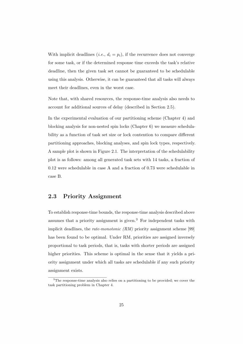
In the experimental evaluation of our partitioning scheme (Chapter 4) and
blocking analysis for non-nested spin locks (Chapter 6) we measure schedula-
bility as a function of task set size or lock contention to compare different
partitioning approaches, blocking analyses, and spin lock types, respectively.
A sample plot is shown in Figure 2.1. The interpretation of the schedulability
plot is as follows: among all generated task sets with 14 tasks, a fraction of
0.12 were schedulable in case A and a fraction of 0.73 were schedulable in
case B.
2.3 Priority Assignment
To establish response-time bounds, the response-time analysis described above
assumes that a priority assignment is given.3 For independent tasks with
implicit deadlines, the rate-monotonic (RM) priority assignment scheme [99]
has been found to be optimal. Under RM, priorities are assigned inversely
proportional to task periods, that is, tasks with shorter periods are assigned
higher priorities. This scheme is optimal in the sense that it yields a pri-
ority assignment under which all tasks are schedulable if any such priority
assignment exists.
3The response-time analysis also relies on a partitioning to be provided; we cover thetask partitioning problem in Chapter 4.
25
0 0.1 0.2 0.3 0.4 0.5 0.6 0.7 0.8 0.9
1
2 4 6 8 10 12 14 16 18 20
sched
ula
ble
number of tasks
case Acase B
Figure 2.1: Example schedulability plot: fraction of generated task sets thatare schedulable as a function of task set size.
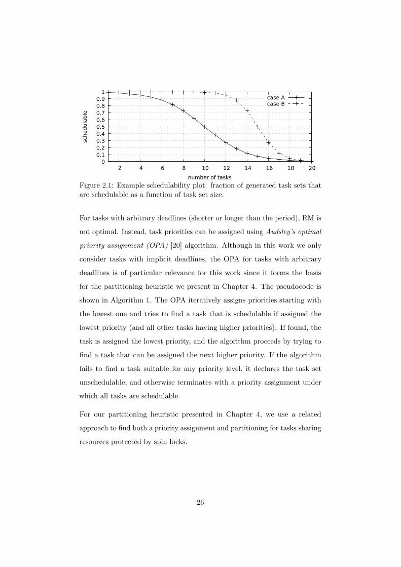
For tasks with arbitrary deadlines (shorter or longer than the period), RM is
not optimal. Instead, task priorities can be assigned using Audsley’s optimal
priority assignment (OPA) [20] algorithm. Although in this work we only
consider tasks with implicit deadlines, the OPA for tasks with arbitrary
deadlines is of particular relevance for this work since it forms the basis
for the partitioning heuristic we present in Chapter 4. The pseudocode is
shown in Algorithm 1. The OPA iteratively assigns priorities starting with
the lowest one and tries to find a task that is schedulable if assigned the
lowest priority (and all other tasks having higher priorities). If found, the
task is assigned the lowest priority, and the algorithm proceeds by trying to
find a task that can be assigned the next higher priority. If the algorithm
fails to find a task suitable for any priority level, it declares the task set
unschedulable, and otherwise terminates with a priority assignment under
which all tasks are schedulable.
For our partitioning heuristic presented in Chapter 4, we use a related
approach to find both a priority assignment and partitioning for tasks sharing
resources protected by spin locks.
26
Algorithm 1 Audsley’s Optimal Priority Assignment (OPA) algorithm.
1: function AssignPriority(τ)2: assign priority 1 to all tasks3: unassigned ← τ4: assigned ← ∅5: for priority π = n down to 1 do6: success ← False7: for each task T ∈ unassigned do8: assign priority π to T9: if T schedulable then
10: unassigned ← unassigned \ T11: assigned ← assigned ∪ T12: success ← True13: break . continue with next priority level14: else15: assign priority 1 to T16: end if17: end for18: if ¬success then19: return unschedulable20: end if21: end for22: return schedulable23: end function
2.4 Mutex Locks and Locking Protocols
Mutex locks are a synchronization mechanism that can be used to ensure
mutual exclusion among concurrent requests (e.g., [60, 61]). We assume
that a unique lock is associated with each shared resource: each global
resource is protected by a spin lock, and each local resource is protected by
a suspension-based lock. For simplicity, we use the notation for a shared
resource to also refer to its associated spin lock in the context of spin lock
operations.
2.4.1 Mutex Lock Programming Interface and Semantics
The basic programming interface for mutex locks defines (at least) operations
to acquire and release a mutex lock. In the remainder of this work, we
denote these operations with acquire(`q) and release(`q) to acquire and
27
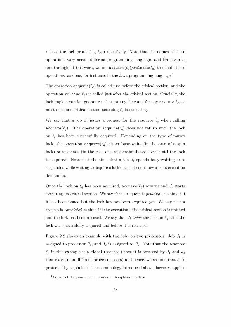
release the lock protecting `q, respectively. Note that the names of these
operations vary across different programming languages and frameworks,
and throughout this work, we use acquire(`q)/release(`q) to denote these
operations, as done, for instance, in the Java programming language.4
The operation acquire(`q) is called just before the critical section, and the
operation release(`q) is called just after the critical section. Crucially, the
lock implementation guarantees that, at any time and for any resource `q, at
most once one critical section accessing `q is executing.
We say that a job Ji issues a request for the resource `q when calling
acquire(`q). The operation acquire(`q) does not return until the lock
on `q has been successfully acquired. Depending on the type of mutex
lock, the operation acquire(`q) either busy-waits (in the case of a spin
lock) or suspends (in the case of a suspension-based lock) until the lock
is acquired. Note that the time that a job Ji spends busy-waiting or is
suspended while waiting to acquire a lock does not count towards its execution
demand ei.
Once the lock on `q has been acquired, acquire(`q) returns and Ji starts
executing its critical section. We say that a request is pending at a time t if
it has been issued but the lock has not been acquired yet. We say that a
request is completed at time t if the execution of its critical section is finished
and the lock has been released. We say that Ji holds the lock on `q after the
lock was successfully acquired and before it is released.
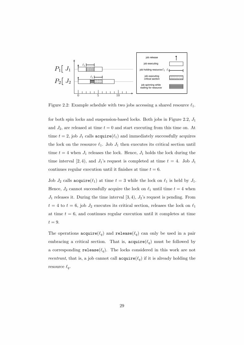
Figure 2.2 shows an example with two jobs on two processors. Job J1 is
assigned to processor P1, and J2 is assigned to P2. Note that the resource
`1 in this example is a global resource (since it is accessed by J1 and J2
that execute on different processor cores) and hence, we assume that `1 is
protected by a spin lock. The terminology introduced above, however, applies
4As part of the java.util.concurrent.Semaphore interface.
28
50 10
J1
J2
P1
P2
job executing
job spinning while waiting for resource
job executingcritical section
job holding resource `1`1
job release
`1
`1
Figure 2.2: Example schedule with two jobs accessing a shared resource `1.
for both spin locks and suspension-based locks. Both jobs in Figure 2.2, J1
and J2, are released at time t = 0 and start executing from this time on. At
time t = 2, job J1 calls acquire(`1) and immediately successfully acquires
the lock on the resource `1. Job J1 then executes its critical section until
time t = 4 when J1 releases the lock. Hence, J1 holds the lock during the
time interval [2, 4), and J1’s request is completed at time t = 4. Job J1
continues regular execution until it finishes at time t = 6.
Job J2 calls acquire(`1) at time t = 3 while the lock on `1 is held by J1.
Hence, J2 cannot successfully acquire the lock on `1 until time t = 4 when
J1 releases it. During the time interval [3, 4), J2’s request is pending. From
t = 4 to t = 6, job J2 executes its critical section, releases the lock on `1
at time t = 6, and continues regular execution until it completes at time
t = 9.
The operations acquire(`q) and release(`q) can only be used in a pair
embracing a critical section. That is, acquire(`q) must be followed by
a corresponding release(`q). The locks considered in this work are not
reentrant, that is, a job cannot call acquire(`q) if it is already holding the
resource `q.
29
2.4.2 Spin Locks
Spin locks are one class of mutex locks that spin (i.e., busy wait) during the
acquire(·) operation until the lock is successfully acquired. In the example
schedule depicted in Figure 2.2, job J2 spins during the time interval [3, 4).
Throughout this work we assume that preemptions are disabled while a
job holds a spin lock. That is, after starting the execution of a critical
section protected by a spin lock, a job is scheduled until the critical section
is completed and the lock is released. While spinning (i.e., after issuing a
request and before successfully acquiring a lock), preemptions may or may
not be allowed depending on the type of spin lock.
The spin lock semantics do not specify in which order conflicting requests
are served. In case multiple requests for the same resource are pending
at the same time, the order in which these pending requests are served is
determined by an ordering policy. In this work, we consider four different
ordering policies:
• FIFO-order (F): Requests are served in the order of the time they were
issued (first come, first serve). Ties between requests issued at the
same time are broken arbitrarily.
• Priority-order (P): Requests are served with respect to a priority
assigned to each request. Priority-ordered locks ensure that each request
can be blocked at most once by a request with lower priority. Ties
between requests issued with the same priority are broken arbitrarily.
• Prio-FIFO-order (PF): Similar to priority-order, requests are ordered
according to their priority, but requests with same priority are served
in FIFO-order.
• Unordered (U): Requests are served in arbitrary order.
30
Similarly, the spin lock semantics do not specify whether preemptions are
allowed while spinning. We consider both options and call a spin lock pre-
emptable (P) if preemptions are allowed while spinning, and non-preemptable
(N) otherwise. For spin locks with preemptable spinning, we assume pre-
emptions while spinning cause a pending request to be cancelled. Cancelled
requests are re-issued once the issuing job resumes execution (and continues
spinning), and the previously issued request is discarded. A request is not
served if the issuing job was preempted (while spinning), and the ordering
policy is enforced with respect to the latest re-issued request (and not with
respect to an earlier issued request later discarded) in case a spinning job is
preempted.
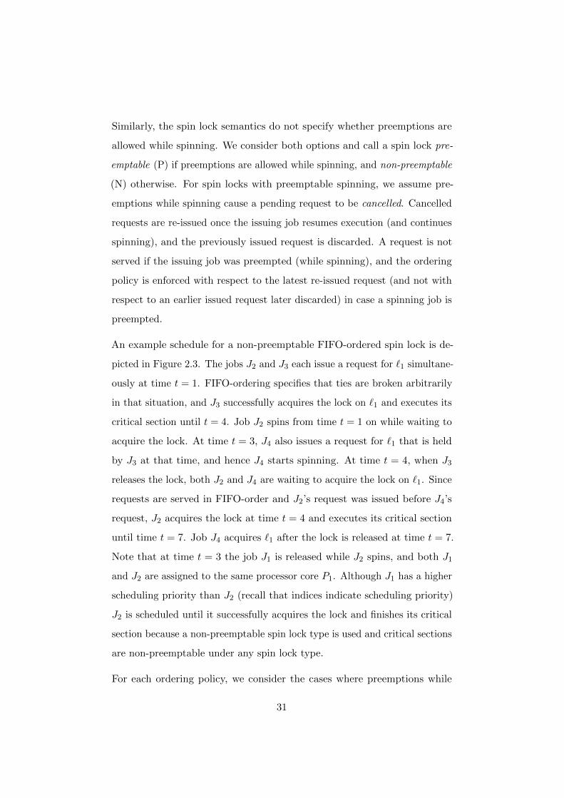
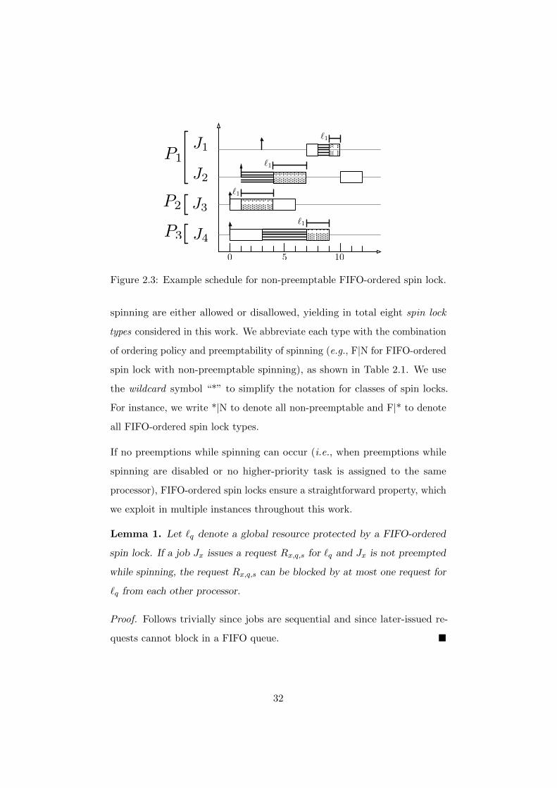
An example schedule for a non-preemptable FIFO-ordered spin lock is de-
picted in Figure 2.3. The jobs J2 and J3 each issue a request for `1 simultane-
ously at time t = 1. FIFO-ordering specifies that ties are broken arbitrarily
in that situation, and J3 successfully acquires the lock on `1 and executes its
critical section until t = 4. Job J2 spins from time t = 1 on while waiting to
acquire the lock. At time t = 3, J4 also issues a request for `1 that is held
by J3 at that time, and hence J4 starts spinning. At time t = 4, when J3
releases the lock, both J2 and J4 are waiting to acquire the lock on `1. Since
requests are served in FIFO-order and J2’s request was issued before J4’s
request, J2 acquires the lock at time t = 4 and executes its critical section
until time t = 7. Job J4 acquires `1 after the lock is released at time t = 7.
Note that at time t = 3 the job J1 is released while J2 spins, and both J1
and J2 are assigned to the same processor core P1. Although J1 has a higher
scheduling priority than J2 (recall that indices indicate scheduling priority)
J2 is scheduled until it successfully acquires the lock and finishes its critical
section because a non-preemptable spin lock type is used and critical sections
are non-preemptable under any spin lock type.
For each ordering policy, we consider the cases where preemptions while
31
50 10
J1
J2
P1
P2
P3 J4
J3
`1
`1
`1
`1
Figure 2.3: Example schedule for non-preemptable FIFO-ordered spin lock.
spinning are either allowed or disallowed, yielding in total eight spin lock
types considered in this work. We abbreviate each type with the combination
of ordering policy and preemptability of spinning (e.g., F|N for FIFO-ordered
spin lock with non-preemptable spinning), as shown in Table 2.1. We use
the wildcard symbol “*” to simplify the notation for classes of spin locks.
For instance, we write *|N to denote all non-preemptable and F|* to denote
all FIFO-ordered spin lock types.
If no preemptions while spinning can occur (i.e., when preemptions while
spinning are disabled or no higher-priority task is assigned to the same
processor), FIFO-ordered spin locks ensure a straightforward property, which
we exploit in multiple instances throughout this work.
Lemma 1. Let `q denote a global resource protected by a FIFO-ordered
spin lock. If a job Jx issues a request Rx,q,s for `q and Jx is not preempted
while spinning, the request Rx,q,s can be blocked by at most one request for
`q from each other processor.
Proof. Follows trivially since jobs are sequential and since later-issued re-
quests cannot block in a FIFO queue.
32
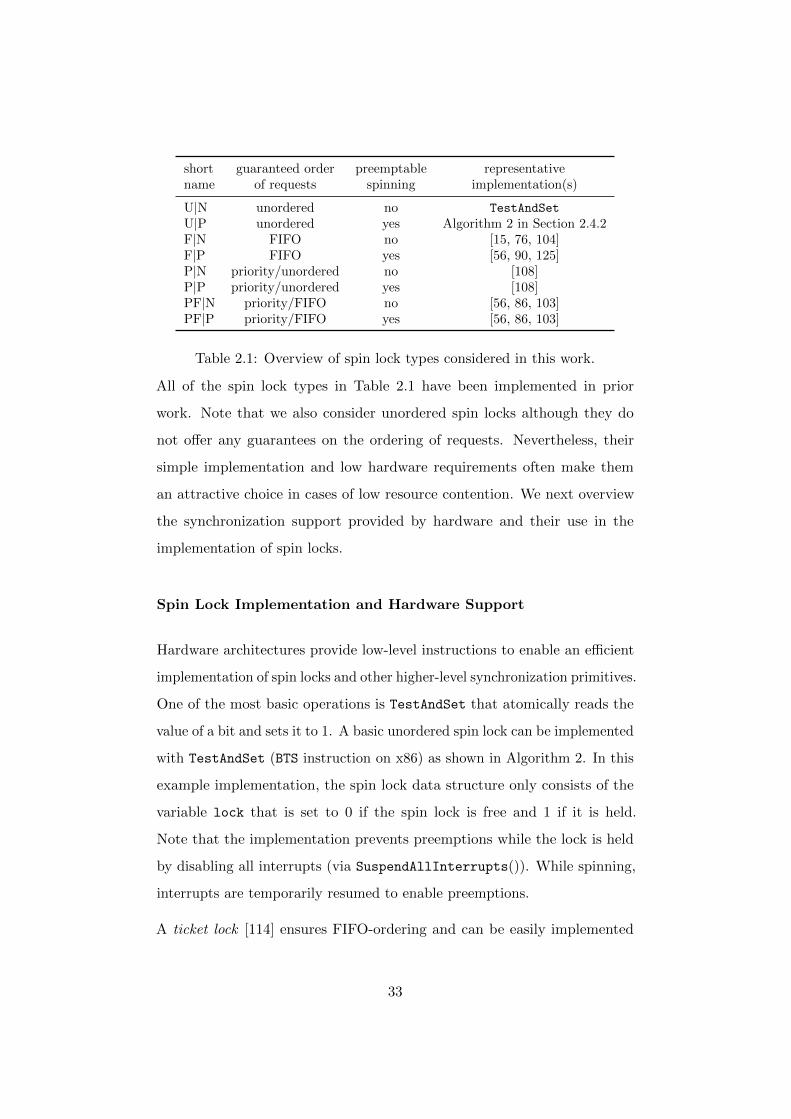
short guaranteed order preemptable representativename of requests spinning implementation(s)
U|N unordered no TestAndSet
U|P unordered yes Algorithm 2 in Section 2.4.2F|N FIFO no [15, 76, 104]F|P FIFO yes [56, 90, 125]P|N priority/unordered no [108]P|P priority/unordered yes [108]PF|N priority/FIFO no [56, 86, 103]PF|P priority/FIFO yes [56, 86, 103]
Table 2.1: Overview of spin lock types considered in this work.
All of the spin lock types in Table 2.1 have been implemented in prior
work. Note that we also consider unordered spin locks although they do
not offer any guarantees on the ordering of requests. Nevertheless, their
simple implementation and low hardware requirements often make them
an attractive choice in cases of low resource contention. We next overview
the synchronization support provided by hardware and their use in the
implementation of spin locks.
Spin Lock Implementation and Hardware Support
Hardware architectures provide low-level instructions to enable an efficient
implementation of spin locks and other higher-level synchronization primitives.
One of the most basic operations is TestAndSet that atomically reads the
value of a bit and sets it to 1. A basic unordered spin lock can be implemented
with TestAndSet (BTS instruction on x86) as shown in Algorithm 2. In this
example implementation, the spin lock data structure only consists of the
variable lock that is set to 0 if the spin lock is free and 1 if it is held.
Note that the implementation prevents preemptions while the lock is held
by disabling all interrupts (via SuspendAllInterrupts()). While spinning,
interrupts are temporarily resumed to enable preemptions.
A ticket lock [114] ensures FIFO-ordering and can be easily implemented
33
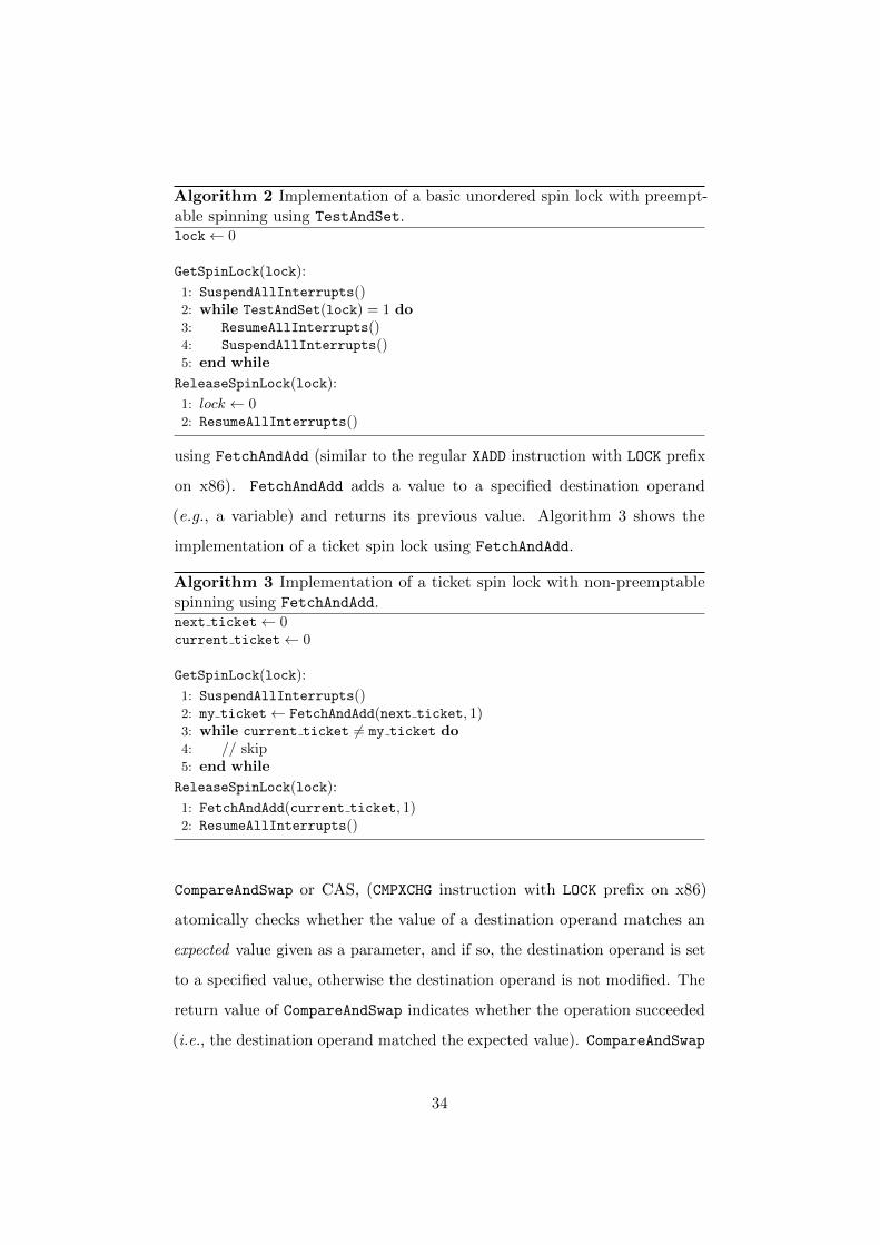
Algorithm 2 Implementation of a basic unordered spin lock with preempt-able spinning using TestAndSet.lock← 0
GetSpinLock(lock):
1: SuspendAllInterrupts()2: while TestAndSet(lock) = 1 do3: ResumeAllInterrupts()4: SuspendAllInterrupts()5: end while
ReleaseSpinLock(lock):
1: lock ← 02: ResumeAllInterrupts()
using FetchAndAdd (similar to the regular XADD instruction with LOCK prefix
on x86). FetchAndAdd adds a value to a specified destination operand
(e.g., a variable) and returns its previous value. Algorithm 3 shows the
implementation of a ticket spin lock using FetchAndAdd.
Algorithm 3 Implementation of a ticket spin lock with non-preemptablespinning using FetchAndAdd.next ticket← 0current ticket← 0
GetSpinLock(lock):
1: SuspendAllInterrupts()2: my ticket← FetchAndAdd(next ticket, 1)3: while current ticket 6= my ticket do4: // skip5: end while
ReleaseSpinLock(lock):
1: FetchAndAdd(current ticket, 1)2: ResumeAllInterrupts()
CompareAndSwap or CAS, (CMPXCHG instruction with LOCK prefix on x86)
atomically checks whether the value of a destination operand matches an
expected value given as a parameter, and if so, the destination operand is set
to a specified value, otherwise the destination operand is not modified. The
return value of CompareAndSwap indicates whether the operation succeeded
(i.e., the destination operand matched the expected value). CompareAndSwap
34

is used to efficiently modify data structures (e.g., a linked list in the spin
lock implementation as proposed by Mellor-Crummey and Scott [104]). The
basic CompareAndSwap instruction operates on a single word, but variants
for two words (double- or multi-word CAS) exist as well.
The implementations shown in Algorithm 2 and Algorithm 3 have hot spots
that can lead to limited performance in case of lock contention. In particular,
the variables lock (in Algorithm 2), next ticket and current ticket (in
Algorithm 3) are not local to any processor and yet frequently accessed from
all spinning processors. This non-locality of frequently accessed memory can
cause significant overhead, and other implementations address this short-
coming with data structures exhibiting better locality (e.g., [15, 76, 104]) or
reducing the use of—comparably expensive—atomic instructions [117].
Without requiring a particular type or implementation, spin locks are man-
dated by the AUTOSAR operating system specification for protecting global
resources. Next, we describe the spin lock API mandated by AUTOSAR,
point out limitations of the API and propose a solution.
Spin Locks in AUTOSAR
AUTOSAR [1] is an operating system specification based on the OSEK [8]
specification developed for embedded control systems (implemented by, e.g.,
[3, 5–7]). AUTOSAR specifically targets automotive embedded systems and
is implemented by a variety of free open-source (e.g., [4] for AUTOSAR
version 3.1) and commercial (e.g., [3, 5]) operating systems. The AUTOSAR
specification mandates the use of a suspension-based locking protocol for
protecting local resources (considered in the next section), and spin locks
for global resources. AUTOSAR does not mandate that spin locks serve
requests in any particular order. For using spin locks, AUTOSAR specifies
the API calls GetSpinlock(<LockID>) and ReleaseSpinlock(<LockID>),
35

which correspond to the operations acquire(·) and release(·) as described
previously.
The API calls GetSpinlock(<LockID>) and ReleaseSpinlock(<LockID>)
alone do not prevent preemptions, neither while spinning nor while executing a
critical section. Preemptions have to be explicitly prevented by (temporarily)
disabling interrupts (that may trigger the release of a higher-priority task,
and hence, a preemption) via separate API calls: SuspendAllInterrupts()
and ResumeAllInterrupts(). Algorithm 4 shows how these API calls can
be combined to implement a non-preemptable lock, maintaining the request
ordering guarantees provided by a spin lock implementation in the particular
OS (recall that AUTOSAR doesn’t specify a particular ordering).
Latency-sensitive tasks may require preemptable locks to avoid blocking due
to spinning lower-priority tasks. Algorithm 4, however, cannot be easily
adapted to allow preemptions while spinning and prevent any preemptions
while executing the critical section. When preemptions are disabled just
after the lock was acquired (i.e., lines 1 and 2 in Algorithm 4 are swapped), a
preemption could still take place just after the lock was acquired and before
preemptions are disabled. In this case, other jobs waiting to gain access the
same resource incur additional delays determined by the regular execution
time of the preempting job. Hence, this approach does not yield a predictable
implementation of a spin lock with preemptable spinning.
Preemptable spin locks can be implemented with the API call
TryToGetSpinlock(<LockID>) specified by AUTOSAR. In contrast to
GetSpinlock(<LockID>), this call does not spin until the lock is acquired,
but tries to acquire the lock without blocking, and then returns a value
indicating whether the attempt was successful. Algorithm 5 shows how this
can be used to implement a spinlock with preemptable spinning. Preemptions
are disabled (line 1) before TryToGetSpinlock(<LockID>) is invoked (line
36
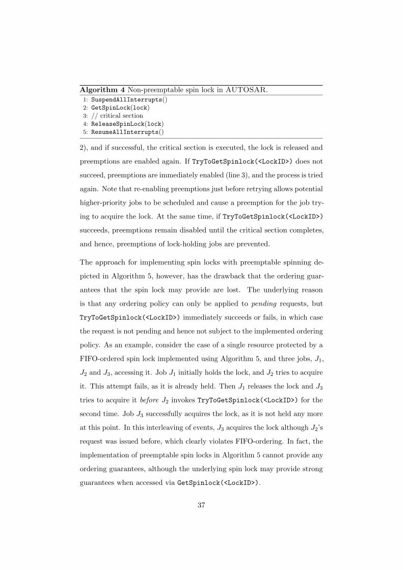
Algorithm 4 Non-preemptable spin lock in AUTOSAR.
1: SuspendAllInterrupts()2: GetSpinLock(lock)3: // critical section4: ReleaseSpinLock(lock)5: ResumeAllInterrupts()
2), and if successful, the critical section is executed, the lock is released and
preemptions are enabled again. If TryToGetSpinlock(<LockID>) does not
succeed, preemptions are immediately enabled (line 3), and the process is tried
again. Note that re-enabling preemptions just before retrying allows potential
higher-priority jobs to be scheduled and cause a preemption for the job try-
ing to acquire the lock. At the same time, if TryToGetSpinlock(<LockID>)
succeeds, preemptions remain disabled until the critical section completes,
and hence, preemptions of lock-holding jobs are prevented.
The approach for implementing spin locks with preemptable spinning de-
picted in Algorithm 5, however, has the drawback that the ordering guar-
antees that the spin lock may provide are lost. The underlying reason
is that any ordering policy can only be applied to pending requests, but
TryToGetSpinlock(<LockID>) immediately succeeds or fails, in which case
the request is not pending and hence not subject to the implemented ordering
policy. As an example, consider the case of a single resource protected by a
FIFO-ordered spin lock implemented using Algorithm 5, and three jobs, J1,
J2 and J3, accessing it. Job J1 initially holds the lock, and J2 tries to acquire
it. This attempt fails, as it is already held. Then J1 releases the lock and J3
tries to acquire it before J2 invokes TryToGetSpinlock(<LockID>) for the
second time. Job J3 successfully acquires the lock, as it is not held any more
at this point. In this interleaving of events, J3 acquires the lock although J2’s
request was issued before, which clearly violates FIFO-ordering. In fact, the
implementation of preemptable spin locks in Algorithm 5 cannot provide any
ordering guarantees, although the underlying spin lock may provide strong
guarantees when accessed via GetSpinlock(<LockID>).
37
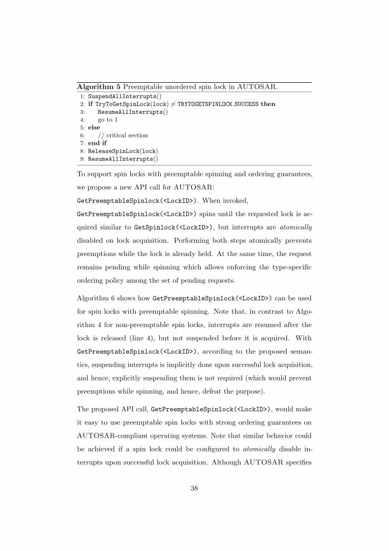
Algorithm 5 Preemptable unordered spin lock in AUTOSAR.
1: SuspendAllInterrupts()2: if TryToGetSpinLock(lock) 6= TRYTOGETSPINLOCK SUCCESS then3: ResumeAllInterrupts()4: go to 15: else6: // critical section7: end if8: ReleaseSpinLock(lock)9: ResumeAllInterrupts()
To support spin locks with preemptable spinning and ordering guarantees,
we propose a new API call for AUTOSAR:
GetPreemptableSpinlock(<LockID>). When invoked,
GetPreemptableSpinlock(<LockID>) spins until the requested lock is ac-
quired similar to GetSpinlock(<LockID>), but interrupts are atomically
disabled on lock acquisition. Performing both steps atomically prevents
preemptions while the lock is already held. At the same time, the request
remains pending while spinning which allows enforcing the type-specific
ordering policy among the set of pending requests.
Algorithm 6 shows how GetPreemptableSpinlock(<LockID>) can be used
for spin locks with preemptable spinning. Note that, in contrast to Algo-
rithm 4 for non-preemptable spin locks, interrupts are resumed after the
lock is released (line 4), but not suspended before it is acquired. With
GetPreemptableSpinlock(<LockID>), according to the proposed seman-
tics, suspending interrupts is implicitly done upon successful lock acquisition,
and hence, explicitly suspending them is not required (which would prevent
preemptions while spinning, and hence, defeat the purpose).
The proposed API call, GetPreemptableSpinlock(<LockID>), would make
it easy to use preemptable spin locks with strong ordering guarantees on
AUTOSAR-compliant operating systems. Note that similar behavior could
be achieved if a spin lock could be configured to atomically disable in-
terrupts upon successful lock acquisition. Although AUTOSAR specifies
38

Algorithm 6 Proposed API for preemptable spin locks.
1: GetPreemptableSpinLock(lock) // atomically disables interrupts on success2: // critical section3: ReleaseSpinLock(lock)4: ResumeAllInterrupts()
an API to configure spin locks to disable interrupts on lock acquisition
(OsSpinlockLockMethod), it does not specify that this is performed atom-
ically, which is crucial to prevent ordering violations as illustrated above.
While AUTOSAR mandates the use of spin locks for protecting global re-
sources, local resources have to be protected by a suspension-based lock.
2.4.3 Suspension-Based Locks
Suspension-based locks provide a programming interface similar to the one
offered by spin locks: the operations acquire(`q) and release(`q) (also
named lock(`q)/unlock(`q) or P(`q)/V(`q)) are called before and after a
critical section, respectively, and the implementation ensures that, for any
resource `q, at any time, the lock on `q can be held by at most one job. The
crucial difference to spin locks is that the operation acquire(`q) does not
spin until the lock is successfully acquired, but rather suspends the calling
job, and hence allows another pending job on the same processor core to be
scheduled.
Suspension-based locks can conceptually also be used for global resources.
However, throughout this work, we assume that suspension-based locks are
only used for local resources, and spin locks are used for global resources, as
mandated by the AUTOSAR specification.
Suspension-based locks are used as part of two classic locking protocols for
uniprocessor systems, the Priority Ceiling Protocol and the Stack Resource
Protocol, which we describe next.
39
The Priority Ceiling Protocol
The Priority Ceiling Protocol (PCP) [121] is a classic real-time locking
protocol designed for uniprocessor systems under fixed-priority schedul-
ing, but it can also be used for local resources in a partitioned multi-
core system. For each local resource `q the PCP defines the priority ceil-
ing Π(`q) to be the highest scheduling priority of any task accessing `q:
Π(`q) = minTiπi|Ni,q > 0. Further, the PCP defines the system ceiling
Π(t) at time t to be the maximum priority ceiling of any resource held
at time t: Π(t) = min`qΠ(`q)| `q is locked at time t ∪ n + 1
, where
Π(t) = n+ 1 indicates that no resource is locked at time t.
The PCP (simplified without support for nested requests) defines the following
locking rules:
• If a job Ji requests the resource `q and Ji’s priority i is higher than the
system ceiling at time t, i.e., i < Π(t), then Ji’s request is served and
Ji can enter its critical section. If Ji’s priority is at most the system
ceiling at time t, i.e., i ≥ Π(t), then Ji’s request is blocked.
• If a job Ji holds a resource `q and a higher-priority job Jh (with
h < i) requests resource `q, then Ji inherits Jh’s higher priority until
Ji releases `q.
Jobs are scheduled according to a fixed-priority scheduler, taking into account
that jobs may temporarily inherit higher scheduling priorities according the
locking rules stated above. Notably, in contrast to critical sections protected
by spin locks, the PCP allows preemptions during the execution of critical
sections.
The schedule in Figure 2.4 illustrates the behavior of the PCP. At time t = 1
the job J3, acquires the lock on resource `1 and starts executing its critical
section. The job J2 is released at time t = 2 and preempts J3 since J2 has a
40
50 10
J1
J2P1
J3
`1 job executing
job executingcritical section
job holding resource `1`1
job release
`1 job suspended while waiting for resource
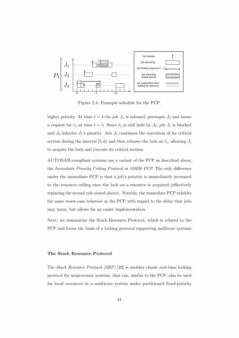
Figure 2.4: Example schedule for the PCP.
higher priority. At time t = 4 the job J1 is released, preempts J2 and issues
a request for `1 at time t = 5. Since `1 is still held by J3, job J1 is blocked
and J3 inherits J1’s priority. Job J3 continues the execution of its critical
section during the interval [5, 6) and then releases the lock on `1, allowing J1
to acquire the lock and execute its critical section.
AUTOSAR-compliant systems use a variant of the PCP as described above,
the Immediate Priority Ceiling Protocol or OSEK PCP. The only difference
under the immediate PCP is that a job’s priority is immediately increased
to the resource ceiling once the lock on a resource is acquired (effectively
replacing the second rule stated above). Notably, the immediate PCP exhibits
the same worst-case behavior as the PCP with regard to the delay that jobs
may incur, but allows for an easier implementation.
Next, we summarize the Stack Resource Protocol, which is related to the
PCP and forms the basis of a locking protocol supporting multicore systems.
The Stack Resource Protocol
The Stack Resource Protocol (SRP) [23] is another classic real-time locking
protocol for uniprocessor systems, that can, similar to the PCP, also be used
for local resources in a multicore system under partitioned fixed-priority
41

scheduling. For the sake of simplicity, we describe a simplified variant of the
SRP that omits the concept of preemption levels as used in [23], which is
required for the analysis of the SRP under EDF scheduling. The SRP is based
on notion of resource ceilings, similar to the PCP. The SRP, however, aims
to reduce the number of context switches between jobs with the following
locking rule:
• A newly released job Ji may only start executing at time t if i < Π(t).
This rule ensures that, at the time Ji starts executing, all (local) resources
that Ji might access are available. Compared with the PCP, this rule of the
SRP causes a job to incur delay before starting to execute, while under the
PCP the delay is incurred when Ji issues a request for a resource that is
already held. The total worst-case delay that a job can incur under the SRP,
however, is the same as under the PCP (and hence also the same as under
the immediate PCP used in AUTOSAR-compliant systems5).
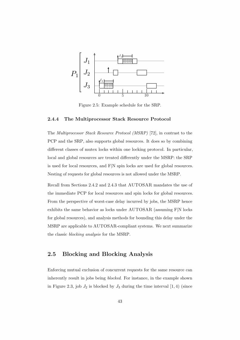
As an example, consider the jobs and their arrival times in Figure 2.5. At
time t = 2, when J2 is released, the system ceiling Π(2) is Π(2) = 1, since J3
holds resource `1, which is also accessed by J1. Hence, since 2 6< Π(2) holds,
J2 does not start executing until time t = 3, when J3 releases its lock on `1
and the system ceiling is lowered to Π(3) = n+ 1 = 4. At time t = 4, job J1
is released and starts executing immediately (preempting J2) since Π(4) = 4
and hence 1 < Π(4).
The SRP is used as part of the Multiprocessor Stack Resource Protocol, a
locking protocol suitable for both local and global resources under partitioned
fixed-priority.
5In fact, the immediate PCP can be considered to be an implementation of the SRPsince the immediate priority increase effectively ensures the locking rule we stated for theSRP.
42
50 10
J1
J2P1
J3
`1
`1
Figure 2.5: Example schedule for the SRP.
2.4.4 The Multiprocessor Stack Resource Protocol
The Multiprocessor Stack Resource Protocol (MSRP) [72], in contrast to the
PCP and the SRP, also supports global resources. It does so by combining
different classes of mutex locks within one locking protocol. In particular,
local and global resources are treated differently under the MSRP: the SRP
is used for local resources, and F|N spin locks are used for global resources.
Nesting of requests for global resources is not allowed under the MSRP.
Recall from Sections 2.4.2 and 2.4.3 that AUTOSAR mandates the use of
the immediate PCP for local resources and spin locks for global resources.
From the perspective of worst-case delay incurred by jobs, the MSRP hence
exhibits the same behavior as locks under AUTOSAR (assuming F|N locks
for global resources), and analysis methods for bounding this delay under the
MSRP are applicable to AUTOSAR-compliant systems. We next summarize
the classic blocking analysis for the MSRP.
2.5 Blocking and Blocking Analysis
Enforcing mutual exclusion of concurrent requests for the same resource can
inherently result in jobs being blocked. For instance, in the example shown
in Figure 2.3, job J2 is blocked by J3 during the time interval [1, 4) (since
43
during that time J3 holds `1, which J2 tries to acquire), and J4 is blocked
by both J2 and J3 during the interval [3, 7).
Such blocking effects contribute to the response time of each task, and hence,
impact the schedulability of a task set. The worst-case blocking duration
depends on the task set properties and how it is deployed on the system,
namely
• the requests for shared resources issued by tasks,
• the mapping of tasks to processor cores,
• the scheduling priority assigned to each task,
• the type of lock used and type-specific parameters (if any) such as
request priority.
The goal of a blocking analysis is to take these factors into account and
derive safe bounds on the blocking duration that hold for any possible
schedule. These blocking bounds can then be incorporated into a response-
time analysis (described in Section 2.2 for independent task sets) to establish
schedulability.
The MSRP, as described in Section 2.4.4, uses the SRP for local resources
and F|N locks for global resources. Gai et al . [72] proposed a blocking
analysis for the MSRP that distinguishes between these two cases, and hence,
implicitly incorporates a blocking analysis for F|N locks. Notably, for the
other spin lock types considered in this thesis (see Table 2.1 for an overview)
no blocking analysis was available prior to the method presented in this
thesis (Chapter 6). Next, we summarize the blocking analysis for the MSRP
originally proposed by Gai et al . [72].
44
2.5.1 Blocking Analysis for the MSRP
Under the MSRP, three types of blocking can be distinguished: local blocking
due to the SRP, and non-preemptive blocking and remote blocking due to
spin locks. The former two types both cause priority inversions [40, 121],
whereas the latter results in spinning. We briefly review the analysis of each
blocking type.
Local Blocking A job Ji incurs local blocking under the SRP if, at the
time of Ji’s release, a job of a local lower-priority task Tl (i.e., i < l) executes
a request for a local resource `q with Π(`q) ≤ i. Under the SRP, Tl’s request
for `q causes the system ceiling Π(t) to be set to at least Π(`q). If Ti releases
a job while Tl is holding `q, Ji is delayed since Π(t) ≤ i, and hence Ji is
blocked by Tl’s job.
Each job of Ti can be locally blocked at most once (upon release) for a
duration of at most βloci time units, where
βloci = maxTl,qLl,q|Nl,q > 0 ∧Π(`q) ≤ i < l ∧ `q is local.
Here and in the following, we define max(∅) , 0 for brevity of notation.
Remote Blocking Since the MSRP uses F|N spin locks, a job Ji that
requested a global resource `q spins non-preemptably until successfully ac-
quiring the lock on `q. Due to the strong progress guarantee of F|N locks,
each request for `q can be blocked at by at most one request for `q from each
other processor core. Hence, the maximum spin time per request, denoted
as Si,q, is bounded by the sum of the maximum critical section lengths on
45
each other processor (with respect to `q):
Si,q =
∑
Pk 6=P (Ti)
maxLx,q|P (Tx) = Pk if Ni,q > 0,
0 if Ni,q = 0.
Since Si,q bounds the spin time for each of Ji’s request for `q, the total spin
time βremi can be bounded by the sum of spin times for each of Ji’s requests:
βremi =∑
`qNi,q · Si,q.
Non-Preemptive Blocking A local lower-priority job Jl spinning or
executing non-preemptably can cause a job of Ti become blocked upon
release. The maximum duration βNPi of such blocking is bounded by Tl’s
worst-case spin time and critical section length for a single request:
βNPi = max
Sl,q + Ll,q | P (Ti) = P (Tl) ∧ i < l ∧ `q is global
.
The blocking bounds βloci , βremi and βNPi can be incorporated into a response-
time analysis to derive bounds on the response time.
Schedulability Analysis The response-time analysis for independent task
sets in Equation (2.1) can be extended to account for the blocking under the
MSRP. Under the MSRP, a safe bound on Ti’s response time ri is given by
a solution to the following recurrence [72]:
ri = ei + βremi + maxβNPi , βloci
+
∑h<i
P (Ti)=P (Th)
⌈riph
⌉· e′h, (2.2)
where e′h = eh + βremh denotes Th’s inflated execution cost. The method
of execution time inflation to account for blocking in the blocking analysis
is revisited in Section 6.2, where we point out inherent drawbacks in that
46
approach and present an analysis method to overcome them. Similar to
independent task sets, the schedulability of a task set with shared resources
protected using the MSRP can be established by comparing each task’s
response time and deadline: a task Ti is schedulable if ri ≤ di.
The analysis for the MSRP summarized above is computationally inexpensive,
and so is our spin lock analysis approach for non-nested spin locks presented
in Chapter 6 (albeit more expensive). The blocking analysis for nested spin
locks, in contrast, is a substantially more difficult problem, as we show in
Chapter 7. The difficulty of carrying out a blocking analysis, or solving any
other computational problem, can be characterized as the computational
complexity of the problem. To reason about the complexity of the blocking
analysis problem, we provide background on computational complexity in
the following.
2.6 Computational Complexity
The difficulty of computational problems, such as finding blocking bounds,
is studied as part of computational complexity theory. The difficulty of such
problems is studied independently of actual algorithms solving them, but
rather focusing on the abstract problem itself. In this work we consider two
types of computational problems: combinatorial (or discrete) optimization
problems and decision problems [17].
Combinatorial optimization problems ask for a minimum (or maximum)
solution among a set of feasible solutions. As an example of a combinatorial
optimization problem, consider the problem of computing the distance be-
tween two vertices in a graph, that is, the minimum length of a path between
two vertices (if such a path exists).
For decision problems the solution is always a truth value (i.e., of Boolean
47
form: True or False, 1 or 0). An example of a decision problem is a variant of
the previous problem, namely the problem of deciding whether the distance
between two vertices in a graph is at most a given length. Both variants are
closely related, and in Chapter 7 we consider both the optimization and the
decision variants of the blocking analysis problem to obtain our hardness
results.
The difficulty of a problem can be characterized in terms of the resources
required to solve it, such as computation time. The time complexity of a
computational problem is the minimum asymptotic worst-case number of
simple operations or steps (such as CPU instructions or transitions taken by
a Turing machine) required by any algorithm to find a solution [17]. Note
that studying the complexity of a problem does not require the knowledge of
any concrete algorithm actually solving it. The complexity of problems can
be compared by means of reductions.
2.6.1 Reductions
Let X and Y denote two computational problems. Intuitively, if a solution to
problem X can be obtained by solving Y instead (and potentially performing
some additional work), then problem Y is at least as difficult as problem X.
In that case, we say that problem X can be reduced to Y [17, Ch. 2.2]. In this
work, we make use of polynomial-time reductions. That is, reductions that,
for some polynomial function poly(n) of n, take at most poly(n) time for any
input of size n. We use two different types of polynomial-time reductions:
Turing reductions (Section 7.3.3) and many-one reductions (Sections 7.3.2,
7.4 and 7.5).
48
Turing Reductions
Let X and Y be decision problems.6 A reduction from X to Y is a polynomial-
time Turing reduction [54] if and only if for any input x to X of size n
• the reduction solves the instance X(x) by
• using at most a polynomial number of instances of Y with respect to
n, and
• performing at most a polynomial number of steps with respect to n
outside of invocations of Y .
Polynomial-time Turing reductions are also known as Cook reductions.
As an example, let X denote the problem of deciding whether in a given
undirected graph G = (V,E) there exists an edge e with e ∈ E contained
in all paths between two given distinct vertices v1 and v2 with v1, v2 ⊆ V
and v1 6= v2. That is, X is the problem of deciding whether there is a bridge
(as defined, e.g., in [34]) between v1 and v2. Formally:
X: Test Bridge Exists
Input undirected connected graph G = (V,E), vertices v1 and v2 with
v1, v2 ⊆ V ∧ v1 6= v2
Output True if and only if there is an edge e with e ∈ E such that all
paths p = v1, . . . , v2 in G contain e
Further, let Y denote the problem of deciding whether two vertices v1 and
v2 are disconnected in a given graph G. Formally:
6Turing reductions can be applied to other types of problems (e.g., function problems)as well, but for the sake of simplicity, we focus on decision problems here.
49

Y : Test Disconnected
Input undirected graph G = (V,E), vertices v1 and v2 with v1, v2 ⊆
V ∧ v1 6= v2.
Output True if and only if no path p = v1, . . . , v2 exists in G.
A (valid albeit naive) Turing reduction from X to Y can be constructed as
follows: for each edge e ∈ E (of which there are at most |V |2), construct
the graph G′ = (V,E′) with E′ = E \ e, and solve the problem instance
Y (G′, v1, v2). If Y (G′, v1, v2) returns True for any edge e (i.e., there is no
path between v1 and v2 in G′), then return True as well (since the removal
of edge e disconnects v1 and v2). Otherwise, return False (since any single
edge can be removed without disconnecting v1 and v2, and hence there is no
bridge). Note that this reduction relies on solving multiple instances of the
problem Y (one for each edge) to solve X.
Many-One Reductions
Let X and Y be decision problems, and let X(x) denote the instance of
X applied to the input x. A reduction from X to Y is a polynomial-time
many-one reduction [89] if and only if, for any input x to X, the reduction
produces an input y to Y within polynomial time with respect to the size of x
such that Y (y) yields the solution to the problem instance X(x). Many-one
reductions are also known as Karp reductions.
Note that a many-one reduction only transforms X’s input x, and exactly
one instance of Y is invoked to solve the problem instance X(x). Many-one
reductions are therefore special cases of Turing reductions (which allow a
polynomial number of invocations of Y ).
As an example for a many-one reduction, let X ′ denote the problem of
deciding whether in a given undirected connected graph G = (V,E) all paths
50
between two given vertices v1 and v2 with v1, v2 ⊆ V and v1 6= v2 contain
a given edge e with e ∈ E. That is, X ′ is the problem of deciding whether e
is a bridge between v1 and v2. Formally, let X ′ be defined as follows:
X ′: Test Bridge
Input undirected connected graph G = (V,E), vertices v1 and v2 with
v1, v2 ⊆ V ∧ v1 6= v2, edge e with e ∈ E.
Output True if and only if all paths p = v1, . . . , v2 in G contain e.
Let Y be defined as above, that is, Y is the problem of deciding whether
two vertices in a given graph are disconnected (i.e., no path between them
exists). Then a many-one reduction from X ′ to Y can be constructed as
follows: for a given instance X ′(G, v1, v2, e), construct the graph G′ = (V,E′)
with E′ = E \ e, and return the solution of Y (G′, v1, v2). If the outcome of
Y (G′, v1, v2) is False, then there is a path in G between v1 and v2 that does
not contain e, and hence e is not a bridge. If the outcome of Y (G′, v1, v2)
is True, then e is a bridge between v1 and v2 in G since these vertices
are disconnected as e is removed. Hence, the construction is a many-one
reduction from X ′ to Y .
2.6.2 Complexity Classes
Problems can be categorized into complexity classes based on the compu-
tational resources (i.e., time or space) required to solve them. For decision
problems, the complexity classes P and NP (among a variety of others that
are beyond the scope of this work) have been widely studied. The classes P
and NP are defined as follows:
• P : The set of decision problems that, given an input of size n, can be
solved by a deterministic Turing machine in poly(n) time.
• NP : The set of decision problems that, given an input of size n, can
51
be solved by a non-deterministic Turing machine in poly(n) time.
Note that the class P is contained in NP , since any computation carried out
by a deterministic Turing machine can be carried out by a non-deterministic
Turing machine as well. The question whether these two classes are equal,
that is, whether P =NP holds true or not, is still open [54].
2.6.3 NP-Hardness and NP-Completeness
The problems contained in the same complexity class may differ in difficulty.
To express that a problem X is one of the most difficult problems in NP ,
the problem X is called NP-complete (with respect to a specific type of
reduction). Formally, X is called NP -complete [54, 89, 91] if and only if
• X is in NP , and
• every problem in NP can be reduced to X within polynomial time.
If the latter condition is satisfied, X is at least as difficult as the most difficult
problems in NP , and in this case, X is called NP-hard. Hence, a problem X
is NP -complete if it is NP -hard and also contained in NP .
The complexity of NP -hard problems with numerical input can be further
characterized as strongly or weakly NP -hard. A problem X is called strongly
NP-hard (or NP-hard in the strong sense) if it is NP-hard even when the
numerical input is polynomially bounded in the input size [73]. This is
equivalent to NP -hardness of a problem when assuming that numerical
input is represented in unary form (rather than binary), in which case the
numerical values are naturally polynomially bounded by their representation
size. A problem X that is NP -hard but not strongly NP -hard is called
weakly NP-hard. NP -hard problems without numerical input are considered
strongly NP-hard.
52

2.6.4 Classic Combinatorial Problems
Karp compiled a collection of combinatorial problems [89], which are now
known as Karp’s 21 NP-complete problems. A plenitude of problems have
since been established to be NP -complete, and in the following we briefly
summarize two classic NP -complete problems of relevance to this work.
The Bin-Packing Problem
The bin-packing problem is strongly NP -hard and asks how many bins
are required to fit a number of items of varying size. Formally, let A ,
a1, . . . , an denote a set of items, and let s(ai) denote the size of item ai
that ranges in (0, 1]. For a given set A and item sizes s(·), the bin-packing
problem asks how many bins are required such that
• each item is assigned to exactly one bin, and
• the sum of the sizes of all items assigned to the same bin does not
exceed 1.
The decision variant of the problem [52] takes an additional numeric param-
eter k and asks whether it is possible to fit the items in A with sizes s(·)
into k bins such that the above conditions hold. The decision variant has
been shown to be strongly NP -complete. As we explain in Section 3.2.2,
the bin-packing problem is related to the partitioning problem, a problem
inherent in P-FP scheduling.
The Multiple Choice Matching Problem
The multiple choice matching (MCM) problem [74, GT55] is a strongly
NP -complete [83] graph matching problem. The MCM takes as input
an undirected graph G = (V,E), disjoint edge partitions E1, . . . , Ej with
53
E1∪· · ·∪Ej = E, and a positive integer k. The problem is to decide whether
there exists a subset E′ with E′ ⊆ E and |E′| ≥ k such that E′ contains at
most one edge from each edge partition: ∀i, 1 ≤ i ≤ j : |Ei ∩ E′| ≤ 1. In
Chapter 7 we use the MCM problem to obtain our hardness result for the
blocking analysis of nested locks.
2.6.5 Approximation Schemes
Approximating the solution to an optimization problem can be easier than
computing the exact solution. Approximation schemes differ in computational
complexity and in the worst-case discrepancy between approximate and
exact solution. One type of approximation algorithm is a polynomial-time
approximation scheme (PTAS) that, for a fixed parameter ε with ε > 0,
computes a solution that is within a factor of (1 + ε) for minimization
problems (or (1 − ε) for maximization problems) in polynomial time with
respect to the input size. Notably, the run time of a PTAS can differ for
different values of ε, and the run time is not required to be polynomial with
respect to 1/ε. A PTAS with a run time that is polynomial in both n and
1/ε is called fully polynomial-time approximation scheme (FPTAS).
2.7 Overheads
In a real system, tasks are subject to overheads such as context switch costs or
the loss of cache affinity when preempted. We assume that all non-negligible
overheads have already been factored into the relevant task parameters (i.e.,
mainly ei and each Li,q) using standard accounting techniques (see [43, Chs.
3 and 7] for a detailed discussion).
54
Chapter 3
Related Work
3.1 Task Models
In this work, we assume the sporadic task model [106]. Other models
have been proposed as well, differing in expressiveness and the difficulty of
analyzing them. The periodic task model [99] is more restrictive than the
sporadic task model in that tasks release jobs in regular intervals (rather
than with a minimum separation between consecutive jobs). Other task
models allow expressing different job release patterns: e.g., the event-stream
model [12, 77] allows specifying bounds on the number of job releases per time
interval rather than minimum separation between jobs, and the generalized
multiframe model [107] allows encoding different execution times for jobs of
the same task.
More recent task model proposals based on directed graphs (e.g., [124]) also
allow encoding different inter-arrival times between different types of jobs.
An overview of different graph-based task models for uniprocessor systems is
provided by Stigge and Yi [123]. Multicore systems, in contrast to unipro-
cessor systems, enable parallel execution, and various task models have been
55
presented to express concurrency and opportunities for parallelism within one
task. For instance, task models for capturing synchronous parallel tasks (e.g.,
in fork-join parallelism or parallel for loops in OpenMP and other languages)
have been presented [93, 118]. Baruah et al . and Bonifaci et al . presented
generalized task models for parallel computations [29, 35]. Focusing on the
engineering aspect of embedded systems, Giotto [80, 81] provides an abstract
programming model for control applications that supports communicating
periodic tasks, as well as sensors and actuators. Notably, Giotto programs
capture functionality and timing-requirements in a platform-independent way,
and can be compiled for platforms with different hardware characteristics or
scheduling approaches.
Discovering the task set properties that can be expressed in a task model
is challenging on its own. Task properties such as deadline and period
(or minimum inter-arrival time) can often be inferred from the application
requirements and physical properties of the given system. In contrast,
deriving execution time bounds is challenging [136]. Overviews of methods
for worst-case execution time analysis are provided by Wilhelm et al . [137] and
Abella et al . [11]. Measuring the execution times in the actual system [96, 111]
is one option, but does not guarantee that the worst case will be observed.
Static analysis, e.g., [49, 50, 84, 97, 138, 139], relies on a model of the
hardware architecture and analytically finding the execution path exhibiting
the longest execution time.
A different line of research aims to make the execution more predictable [21,
127], which benefits approaches both based on measurement and static
analysis to find worst-case execution time bounds. This requires hardware
architectures with predictable timing behavior [63, 98, 100, 120, 129] and
programming languages with explicit timing semantics (e.g., [14] tailored for
PRET architectures [98]).
56
3.2 Priority Assignment and Partitioning
P-FP scheduling, as mandated, for instance by operating systems complying
to the AUTOSAR [1] operating system specification, inherently requires
each task to be mapped to one processor core, and assigned a scheduling
priority. The problem of assigning priorities has already been studied in the
context of uniprocessor systems under FP scheduling.
3.2.1 Priority Assignment for FP
For independent periodic tasks with implicit deadlines (i.e., relative deadlines
are equal to the period) and synchronous release (i.e., all tasks release a
job simultaneously release a job at system start), Liu and Layland found
that assigning priorities inversely proportional to task periods (i.e., tasks
with shorter periods are assigned higher priorities) is optimal [99]. That is,
if there exists any task-level priority assignment such that all deadlines are
guaranteed to be met, then all deadlines will be met under this rate-monotonic
(RM) priority assignment as well.
For periodic tasks with constrained deadlines (i.e., relative deadlines do
not exceed the period), Leung and Whitehead have shown that a deadline-
monotonic (DM) priority assignment scheme is optimal [95]. Audsley et al .
show that DM priority assignment is also optimal for sporadic tasks [18]. For
periodic tasks with asynchronous release and arbitrary deadlines, Audsley
showed that neither RM nor DM are optimal [20], and presented an optimal
algorithm for assigning priorities. We summarize this algorithm called
Audsley’s optimal priority assignment (OPA) in Section 2.3. The OPA
forms the basis for our partitioning heuristic presented in Chapter 4. A
recent overview of priority assignment techniques is provided by Davis
et al . [57].
57
3.2.2 Partitioning for P-FP
Partitioned scheduling requires the partitioning of the task set, that is, each
task has to be mapped to one processor core. This partitioning problem
resembles an instance of the classic bin-packing problem (e.g., [74]), which is
known to be strongly NP -complete [89]. For independent tasks, Baruah [31]
and Baruah and Bini [27] presented approaches for solving the partitioning
problem based on Integer Linear Programming (ILP) under EDF and FP
scheduling. To avoid the inherent complexity of solving the partitioning
problem exactly, well-performing (albeit potentially non-optimal) bin-packing
heuristics exist [85], and they have also been applied to the partitioning
problem (e.g., [25, 30, 45, 53, 59, 70, 71, 102]).
Chattopadhyay and Baruah presented a partitioning approach for EDF
scheduling that does not rely on bin-packing heuristics: lookup-tables with a
configurable accuracy parameter are pre-computed offline for each system
platform, which can then be used to efficiently partition tasks for EDF
scheduling [48]. A PTAS (summarized in Section 2.6.5) for partitioning
under EDF scheduling was presented by Baruah [26]. Apart from timing
aspects, the partitioning problem has also been studied with a focus on other
objectives, such as energy efficiency [22] and fault tolerance [69].
Resource sharing complicates the partitioning problem since jobs can interfere
across processor boundaries on resource contention. Generic bin-packing
heuristics do not account for these effects, and hence, bin-packing heuristics
that are oblivious to resource sharing can be inefficient in such settings.
For task sets with precedence constraints, Zheng et al . presented an ILP-based
approach that takes into account interference due to an implicitly shared
resource, a shared bus [143]. Zheng and Di Natale incorporated blocking
due to local (i.e., resources shared among tasks from only a single processor)
58
resources into an ILP-based partitioning approach [142]. Lakshmanan et al .
presented a partitioning heuristic [92] for explicitly shared resources protected
by the MPCP [113], a suspension-based multiprocessor real-time locking
protocol. This heuristic aims to group tasks sharing the same resources
and tries to assign these groups to the same processor. A similar approach
was presented by Nemati et al . with BPA [109], a partitioning heuristic
for the MPCP that incorporates advanced cost heuristics to determine how
groups of tasks can be split up with low overall blocking. These sharing-aware
heuristics tailored to a specific locking protocol can often successfully produce
a valid partitioning (i.e., a partitioning under which all tasks are schedulable)
where sharing-oblivious heuristics fail. However, these heuristics are specific
to the MPCP and are not directly applicable to spin locks. In Chapter 4,
we present an efficient partitioning heuristic for spin locks and an optimal
ILP-based partitioning approach.
Next, we provide an overview of locking protocols for real-time systems.
3.3 Real-Time Locking Protocols
In Section 2.4, we introduced spin locks as one type of mutex lock, suspension-
based locks being the other type. A variety of different suspension-based
locks have been presented, for instance the classic SRP [23], the PCP [121]
(both summarized in Section 2.4.3), and the Priority Inheritance Protocol
(PIP) [121] for uniprocessor systems. The MSRP [72] presented by Gai
et al . (summarized in Section 2.4.4) supports shared-memory multiprocessor
systems under P-FP scheduling and uses the suspension-based SRP for local
resources and F|N for global resources. Notably, the blocking analysis for
the MSRP presented by Gai et al . [72] hence includes an analysis for F|N
spin locks, which was the first blocking analysis for spin locks under P-FP
scheduling. Devi et al . presented a blocking analysis for F|N spin locks under
59
global scheduling [58] analogously to the analysis presented by Gai et al . for
P-FP scheduling.
Brandenburg presented the holistic blocking analysis [43, Ch. 5] that reduces
the pessimism of prior analyses for F|N spin locks by considering all requests
a single job can issue together.1 All of these analyses rely on execution
time inflation, which is inherently pessimistic. In Chapter 6, we detail this
issue and present a blocking analysis approach that avoids this inherent
pessimism.
Takada and Sakamura presented SPEPP [126], a protocol using F|P locks
under which jobs “help” each other to make progress by letting a blocked job
execute earlier-issued requests from other jobs that were possibly preempted
while spinning. A related approach is taken by the MrsP [46], a variant of
the MSRP presented by Burns and Wellings. In contrast to SPEPP (and the
MSRP), the MrsP permits preemptions during critical sections, but ensures
that a lock-holding job makes progress when preempted (and other jobs are
blocked for the same resource): the lock-holding job can resume execution
on a processor with a different blocked job (by migrating the job), or the
critical section can be re-executed by a blocked job on a different processor
core (assuming critical sections can be committed atomically).
Rajkumar presented the Multiprocessor Priority Ceiling Protocol (MPCP)
that is suspension-based for both local and global resources [112]. For
distributed systems (i.e., without shared memory), Rajkumar et al . presented
the suspension-based DPCP [113].
The FMLP presented by Block et al . [33] distinguishes between long and
short requests, and relies on different techniques depending on the request
length: the FMLP is suspension-based for long requests, and spin-based for
1Recall that under Gai et al .’s analysis for the MSRP, as summarized in Section 2.5.1,the worst-case spin time for each request is bounded, and then multiplied with the numberof requests to obtain the total blocking bound.
60
short requests. In contrast to the DPCP, under which requests are served in
priority-order, the FMLP relies on FIFO-ordering. The FMLP was originally
presented for EDF scheduling, but was later adapted to P-FP scheduling as
well [38].
Brandenburg and Anderson explored the amount of blocking that is inher-
ently unavoidable under any mutex-based locking protocol, and devised
the OMLP [40, 42], a suspension-based locking protocol that is asymptoti-
cally optimal under suspension-oblivious analysis2 in the sense that it limits
blocking to an extent that cannot be avoided under any protocol for global,
partitioned and clustered FP and EDF scheduling. The FMLP+ presented
by Brandenburg [37, 43, Ch. 6.3] improves upon the FMLP and also ensures
optimality under suspension-aware analysis.3 Besides partitioned and global,
the FMLP+ also supports clustered scheduling.
For suspension-based mutex locks under P-FP scheduling, Brandenburg
developed an improved blocking analysis approach [36] based on linear
programming that supports the MPCP, DPCP, FMLP+, and the DFLP [44].
Our blocking analysis for spin locks under P-FP scheduling (Chapter 6) uses
a similar technique based on linear programming.
For G-FP scheduling, Easwaran and Andersson presented the PPCP [62],
a suspension-based locking protocol extending the PCP. Yang et al . sub-
sequently presented an analysis framework for suspension-based locking
protocols under G-FP scheduling [141], that incorporates support for the
PIP [62, 121], PPCP [62], FMLP [33], and the FMLP+ [37]. The analysis
is based on techniques presented by Brandenburg [36] in the context of
suspension-based locks under P-FP scheduling.
2Under suspension-oblivious analysis, suspensions are modeled as execution that occupiesthe processor.
3Under suspension-aware analysis, suspensions are explicitly accounted for and notmodeled as execution.
61
While nesting of requests is allowed under several uniprocessor locking proto-
cols such as the PCP,4 the increased parallelism on multiprocessors makes the
support for nesting in locking protocols challenging. The MDPCP presented
by Chen and Tripathi [51] for periodic tasks under P-EDF scheduling, similar
to the PCP, relies on resource ceilings and only enables rather coarse-grained
locking (to access a single global resource, all global resources accessed by
any task from the same processor must be available).
A different technique to support nesting is the group lock, where resources that
may be nested within each other are organized in a group. To access a single
resource, the corresponding group lock must be obtained, even when other
resources in the group are not used. This approach is employed, for instance,
by the FMLP and the PWLP [13], a locking protocol using preemptable
FIFO-ordered spin locks presented by Alfranseder et al . for global and
partitioned FP and EDF scheduling. The RNLP presented by Ward and
Anderson [130] is a family of spin- and suspension-based locking protocols
supporting nesting without group locks for partitioned, clustered and global
FP and EDF scheduling. Notably, the RNLP ensures asymptotically optimal
blocking. Biondi et al . presented the nFIFO protocol [32], a relaxation of
the classic MSRP, that allows nesting and avoids blocking of non-conflicting
requests. The analysis of the nFIFO protocol presented by Biondi et al . is
partially based on our analysis approach presented in Chapter 6.
3.4 Other Synchronization Primitives
Besides binary (suspension-based) semaphores and spin locks, other synchro-
nization primitives have been presented.
4Note that the simplified version of the PCP summarized in Section 2.4.3 does notsupport nested requests, but the original version as presented in [121] does support nesting.
62
k-Exclusion Locks and Reader-Writer Locks (RW-Locks) extend the notion of
strict mutual exclusion by allowing multiple concurrent requests accessing the
same resource and treating read and write requests differently. k-exclusion
locks are initialized with a value indicating the number of available units, and
at any time, at most k units can be held by jobs (and at most one unit per job).
Notably, when initialized to the value of 1, a k-exclusion lock is semantically
equivalent to a mutex lock if one unit is acquired or released. Brandenburg
and Anderson presented asymptotically optimal suspension-based k-exclusion
locks [41] for clustered scheduling. For partitioned scheduling, Yang et al .
subsequently presented a variant of Brandenburg and Anderson’s k-exclusion
locks [41] that enables enables higher concurrency for requests issued from the
same processor [140]. Elliot and Anderson presented a k-exclusion protocol
tailored to GPUs as resources [67]. Nemitz et al . presented protocols [110]
that allow each job to acquire multiple (up to k) units of the same multi-unit
resource (while maintaining the property that at most k units can be held in
total).
RW-locks are motivated by the observation that there exist types of shared
resources that can be safely read (or accessed in a non-mutating way) by
multiple jobs concurrently, while write requests need to be executed in
isolation from any other requests (either reading or writing). Both spin-
based (e.g., [39, 105]) and suspension-based (e.g., [55]) RW-locks have been
presented. If the expected ratio of read and write accesses is known, the
implementation can be optimized for such access patterns (e.g., [82]). Notably,
RW-locks can be implemented using locking protocols for multi-unit resources
with a suitable choice of resource units to acquire or release as a reader or
writer [16, Ch. 8.1].
When multiple readers or writers are waiting to acquire the same lock,
the implementation can enforce a specific order in which the requests are
served. Most common ordering policies include task-fair ordering, where
63

requests are served in FIFO order [105, 115], and preference ordering, where
either readers or writers are given preference. Brandenburg and Anderson
presented phase-fair reader-writer locks [39]. Phase-fair reader-writer locks
allow for increased concurrency among readers and ensure that a reader is
blocked by at most one writer, yielding an asymptotic reduction in worst-case
blocking. Building upon the RNLP, Ward and Anderson presented the R/W
RNLP [131], a reader-writer variant of the RNLP that supports nesting of
requests.
Besides synchronization primitives to ensure mutual exclusion (e.g., spin
locks), other primitives such as barriers, signals or condition variables have
been studied (e.g., [104]) and are supported in many operating systems,
for instance, POSIX-compliant operating systems [9]. These, however, are
beyond the scope of this work, where we focus on spin locks.
3.5 Complexity of Scheduling Problems
The complexity of scheduling problems has been studied in many aspects over
the past decades (see [122] for a survey of classic results). Intractability results
for a variety of feasibility problems, that is, the problem of deciding whether
a schedule exists such that all deadlines are met, have been established (e.g.,
[28, 66, 94, 106, 116]). Similarly, the complexity of commonly used analysis
techniques has been studied (e.g., [28, 64, 65]). For instance, it has been
shown that the feasibility problem for periodic task sets is strongly NP -
hard [95], and deciding feasibility for task sets using semaphores to ensure
mutual exclusion has been shown to be strongly NP -hard as well [106].
In contrast, the problem of bounding the blocking due to resource contention
without deciding task set schedulability is a much simpler one. In fact, the
blocking analysis problem is simple on uniprocessors under the PCP and
64
SRP [24, 121], where it essentially boils down to the problem of identifying
a longest request issued by a task with lower priority (for a resource with
a sufficiently high resource ceiling, see Section 2.5.1 for details). For the
PIP, a simple dynamic programming approach is described in [101]. Even
on multiprocessors a blocking analysis is tractable if critical sections are not
nested (see our analysis in Chapter 6). Allowing nested critical sections on
multiprocessors, however, gives rise to blocking effects (see Section 7.2) that
prevent local per-processor reasoning about worst-case blocking. In fact,
as we show in Chapter 7, nesting on multiprocessors renders the blocking
analysis problem to be strongly NP -hard.
65
Chapter 4
Partitioning Task Sets
Sharing Resources Protected
by Spin Locks 1
4.1 Introduction
Under P-FP scheduling, each task must be assigned to exactly one processor
core for execution. Finding such such a partitioning, i.e., a mapping of tasks
to processors such that all tasks are schedulable, can be challenging. In
fact, the partitioning problem has been shown to be strongly NP -complete,
but computationally inexpensive bin-packing heuristics can be employed for
partitioning task sets (see Section 3.2.2 for an overview of work related to
the partitioning problem).
While generic bin-packing heuristics are oblivious to shared resources, resource-
aware partitioning heuristics have been developed to account for the blocking
effects as well. For shared resources protected by spin locks, for instance in
1This chapter is based on [135].
66

an AUTOSAR-compliant operating system, prior heuristics often fail to
produce a valid partitioning (i.e., a partitioning under which all deadlines
can be guaranteed to be satisfied) although such partitionings exists. As a
result, developers may be forced to utilize more powerful hardware platforms
(potentially increasing space, weight, energy consumption and cost of the
product) or restructure the application (e.g., by splitting up tasks into smaller
ones) to simplify the problem until a partitioning can be found.
To avoid such waste of resources and better utilize multicore platforms, we
developed two partitioning approaches for systems under P-FP scheduling and
the MSRP for protecting shared resources. The remainder of this chapter
is organized as follows. Section 4.2 overviews both generic bin-packing
heuristics and resource-aware partitioning heuristics, and Section 4.3 makes
the case for an optimal partitioning approach. We present two approaches for
resource-aware partitioning: Section 4.4 presents an optimal approach based
on Mixed Integer Linear Programming (MILP), and Section 4.5 presents a
simple and effective partitioning heuristic. Section 4.6 presents evaluation
results and Section 4.7 concludes this chapter.
4.2 Partitioning Heuristics
As briefly pointed out in Section 3.2.2, task sets can be partitioned for
P-FP scheduling using generic bin-packing heuristics, which are oblivious
to shared resources. In contrast, resource-aware partitioning heuristics take
into account each task’s resource access patterns to find a mapping of tasks
to processor cores. In this section, we overview both classic bin-packing
heuristics and resource-aware partitioning heuristics.
67
Classic Bin-Packing Heuristics
Generic bin-packing heuristics are commonly used to map tasks to processors.
Bin-packing heuristics distribute a set of different objects (tasks) of a given
size (processor utilization) to bins (processors), such that each object is
assigned to exactly one bin and the total size of all objects assigned to a
bin does not exceed the bin’s capacity (all tasks are schedulable). Under
P-EDF scheduling, schedulability can be guaranteed if the total utilization
of tasks assigned to each processor does not exceed 1 (shown in [99] for
uniprocessor systems under EDF scheduling). As a direct consequence, a
partitioning obtained with a bin-packing heuristic ensures schedulability
under P-EDF scheduling. Under P-FP scheduling, however, this is not the
case: a task set can be unschedulable even if the per-processor utilization
does not exceed 1 (in fact, in the general case, a response-time analysis is
required to establish schedulability; see Section 2.2). Before describing a
simple adaptation that enables the use of bin-packing heuristics for P-FP
scheduling, we assume P-EDF scheduling for the sake of simplicity and
summarize basic heuristics.
Commonly used heuristics include the first-fit, next-fit, best-fit and worst-fit
heuristics [85], which we describe in brief. All of them take a sequence of
objects (tasks) of a given size (task utilization) as input. We assume that the
input sequence is sorted in order of decreasing size, which typically results
in a lower number of bins required by these heuristics [85]. Bins initially
have unit-capacity (i.e., a capacity of 1) and can be allocated on demand.
Newly allocated bins are empty (i.e., do not have any objects assigned to
them), and the capacity of a bin is defined as its initial capacity subtracted
by the total size of the objects assigned to it. An object fits into a bin if the
capacity of the bin is at least the object size.
The first-fit heuristic iterates over all bins in the order they were allocated,
68
and assigns the current object to the first bin with sufficient remaining
capacity. If no such bin exists, it allocates a new bin and assigns the current
object to it.
The next-fit is simpler in that it only checks the last allocated bin and
allocates a new bin if the last allocated bin does not have sufficient capacity
to fit the current object. Both the first-fit and next-fit heuristics report a
failure if the maximum number of bins is exceeded.
The best-fit and worst-fit heuristics allocate the maximum number of bins
upfront and then assign each object to a bin such that the remaining capacity
in that bin is minimized or maximized, respectively. If no bin with sufficient
capacity exists, they report a failure.
The any-fit heuristic, which we denote as AF in the following, subsumes all
previously described bin-packing heuristics in that it tries all of them (in the
order worst-fit, best-fit, first-fit, next-fit) and returns the first successfully
computed result.
Each of the bin-packing heuristics above can be used for partitioning task sets
under P-FP scheduling when a schedulability test rather than capacity is used
to determine whether a task fits onto a processor. For instance, the first-fit
heuristic assigns a task to the first processor on which the schedulability
of the newly assigned and all previously assigned tasks can be established.
Analogously, the other heuristics only consider assignments under which
schedulability can be established by means of a schedulability test.
Resource-Aware Partitioning Heuristics
Resource sharing causes blocking effects among tasks (i.e., βloci , βremi and
βNPi in Section 2.5.1) that are not reflected in the notion of a task fitting
into a bin as used by the bin-packing heuristics described above. Resource-
69
aware partitioning heuristics account for these effects and take the resource
access patterns into account when mapping tasks to processors. We outline
the MPCP partitioning heuristic [92] and the Blocking-Aware Partitioning
Algorithm (BPA) [109].
The MPCP partitioning heuristic was proposed by Lakshmanan et al . for
the MPCP [113]. Under the MPCP partitioning heuristic, tasks are assigned
to the same bundle if they share (possibly transitively) a common set of
resources. Bundles are then assigned to processors using the best-fit heuristic.
This leads to tasks accessing the same resources being assigned to the same
processor, if possible, to avoid the need for inter-processor synchronization.
Bundles that do not fit on any processor are broken into multiple smaller
ones, such that one bundle fits as tightly as possible onto the processor
with the highest remaining capacity. Bundles are assigned and broken (if
necessary) until all tasks are assigned.
The BPA is related to the MPCP partitioning heuristic in that it groups
together tasks that access the same resources, and, if possible, assigns all
tasks in the same group to the same processor. Otherwise, task groups are
split and the respective tasks are assigned to different processors. In this
case, for each pair of tasks, the BPA also takes into account the remote
blocking (estimated based on the resource access patterns of each task) that
can result as an effect of assigning tasks accessing the same resource to
different processor cores.
As we describe next, when shared resources are protected by the MSRP,
both generic bin-packing heuristics and the resource-aware heuristics de-
scribed above often fail to produce a partitioning under which all tasks are
schedulable, although such partitionings do exist.
70

4.3 The Case for Optimal Partitioning
Exact partitioning approaches for task sets with shared resources can be
computationally expensive due to the hardness of the underlying bin-packing
problem. This complexity raises the question whether exact approaches can
offer substantial benefit over resource-aware heuristics. To answer this ques-
tion, we conducted an experiment to evaluate whether there exists a potential
that is left unused by heuristics but could be exploited by an exact approach.
To this end, we generated task sets for which a valid partitioning was known
to exist by construction, and hence an exact partitioning approach would
have found a valid partitioning. Then we let resource-oblivious and resource-
aware heuristics partition the same task sets and checked schedulability of
the computed partitionings. Priorities were assigned in a rate-monotonic
fashion [99], and before assigning a task to a processor (i.e., to determine
whether a task “fits”) a response-time schedulability test was applied to rule
out choices that render the task set unschedulable.
Figure 4.1 shows the fraction of schedulable task sets under each partitioning
heuristic depending on the number of tasks in the system. The straight
line at the top of the graph marks the fraction of task sets that can be
successfully partitioned by an exact approach, that is, all task sets as only
partitionable task sets were considered in this experiment. As it is apparent
from Figure 4.1, AF is able to produce valid partitionings for all task sets
consisting of up to 20 tasks. For larger task sets, AF is unable to produce
valid partitionings for a large fraction of the generated task sets although
valid partitionings exist and hence, an optimal partitioning scheme would
have found them. Both the MPCP heuristic and BPA show surprisingly low
schedulability, an effect we revisit in Section 4.6.2.
While Figure 4.1 shows results for specific parameter choices, similar results
can be obtained for many other configurations: if blocking due to resource
71
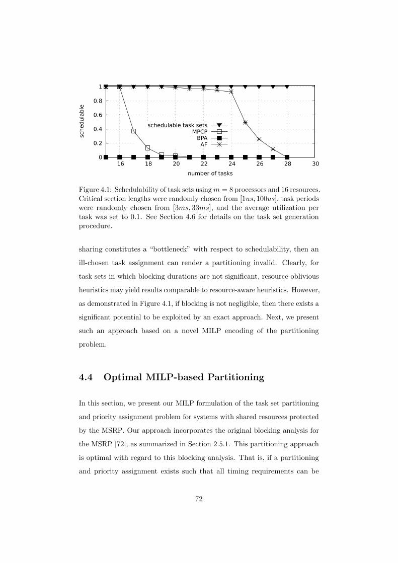
0
0.2
0.4
0.6
0.8
1
16 18 20 22 24 26 28 30
schedula
ble
number of tasks
schedulable task setsMPCP
BPAAF
Figure 4.1: Schedulability of task sets usingm = 8 processors and 16 resources.Critical section lengths were randomly chosen from [1us, 100us], task periodswere randomly chosen from [3ms, 33ms], and the average utilization pertask was set to 0.1. See Section 4.6 for details on the task set generationprocedure.
sharing constitutes a “bottleneck” with respect to schedulability, then an
ill-chosen task assignment can render a partitioning invalid. Clearly, for
task sets in which blocking durations are not significant, resource-oblivious
heuristics may yield results comparable to resource-aware heuristics. However,
as demonstrated in Figure 4.1, if blocking is not negligible, then there exists a
significant potential to be exploited by an exact approach. Next, we present
such an approach based on a novel MILP encoding of the partitioning
problem.
4.4 Optimal MILP-based Partitioning
In this section, we present our MILP formulation of the task set partitioning
and priority assignment problem for systems with shared resources protected
by the MSRP. Our approach incorporates the original blocking analysis for
the MSRP [72], as summarized in Section 2.5.1. This partitioning approach
is optimal with regard to this blocking analysis. That is, if a partitioning
and priority assignment exists such that all timing requirements can be
72
guaranteed to be satisfied under this blocking analysis, our approach is
guaranteed to find such a partitioning and priority assignment. We refer to
such a partitioning and priority assignment as a valid one.
Initially, the MILP formulation does not specify an objective function. That
is, we accept any solution that satisfies all constraints of the MILP, which
allows the objective function to be used to optimize other criteria (such as
the required number of processors, see Section 4.4.4).
We consider the jitter ji, the deadline di, the cost ei, the period pi, the
maximum request length Li,q, and the maximum number of requests Ni,q of
each task Ti to be given task properties that are constants (from a MILP
point of view). Similarly, the number of processors m and the number of
tasks in the task set n are considered constant.
All other terms used in the MILP constraints are variables unless specified
otherwise. At the core of the MILP formulation are four helper variables,
which we define first.
• Ai,k: A binary decision variable that is set to 1 if and only if Ti is
assigned to processor Pk. Since each task must be assigned to exactly
one processor, we have
∀Ti :
m∑k=1
Ai,k = 1. (C1)
• πi,p: A binary decision variable that is set to 1 if and only if Ti is
assigned the priority p. Since each task must be assigned exactly one
priority, we have
∀Ti :n∑p=1
πi,p = 1. (C2)
To ensure unique priorities, we impose the following constraint to
73
enforce that each priority level is assigned to exactly one task:
∀p, 1 ≤ p ≤ n :∑Tx∈τ
πx,p = 1. (C3)
• Vx,i: A binary decision variable that is forced to 1 if Tx and Ti are
assigned to the same processor. If Tx and Ti are assigned to the same
processor k, then Ai,k = Ax,k = 1 holds for some k. The following
constraint exploits this property by forcing Vx,i to 1 in this case:
∀Tx : ∀Ti, Tx 6= Ti : ∀k, 1 ≤ k ≤ m :
Vx,i ≥ 1− (2−Ai,k −Ax,k). (C4)
• Xi,x: A binary decision variable that is set to 1 if and only if Ti has a
higher priority than Tx. We first specify constraints to force Xi,x to 0
if Tx has a higher priority than Ti:
∀Tx : ∀Ti : ∀1 ≤ p ≤ n− 1 :
Xi,x ≤n∑
j=p+1
πx,j + (1− πi,p). (C5)
Constraint C5 is based on the observation that if there exist p1 and
p2 such that πx,p1 = 1 ∧ πi,p2 = 1 ∧ p1 < p2, then 1 − πi,p2 = 0 and
also∑n
j=p+1 πx,j = 0, and thus Constraint C5 reduces to Xi,x ≤ 0 for
p = p2. To ensure that Xi,x is set to 1 if Tx has a lower priority than
Ti, we specify a constraint to enforce that for each pair of tasks Ti and
Tx either Xi,x or Xx,i is set to 1:
∀Tx : ∀Ti, Tx 6= Ti : Xi,x +Xx,i = 1. (C6)
The MILP formulation incorporates Gai et al .’s analysis of the MSRP and
74
enforces that under any valid MILP solution all tasks are indeed schedulable.
That is, for each task Ti, the sum of the release jitter ji and the response
time Ri (a MILP variable) must not exceed the task’s deadline di, which
yields:
∀Ti : ji +Ri ≤ di. (C7)
To constrain the response time Ri, we decompose it into the following
terms:
• ei: the execution cost;
• Bi: the arrival blocking that a job can incur if a local lower-priority
job is spinning or holding a resource;
• Si: the direct and transitive spin delay that a job can incur due to
itself and local higher-priority jobs busy-waiting for a global resource;
and
• Ii: the interference that a job can incur due to local higher-priority
jobs executing non-critical sections.
The response time of a task Ti is the sum of the above terms:
∀Ti : Ri = ei +Bi + Si + Ii. (C8)
Note that, although we specify all of these terms in our MILP formulation
through constraints, we often do not use tight constraints on these terms,
but rather upper or lower bounds that are sufficient for our goal of finding a
valid partitioning. For instance, we impose only lower bounds on the spin
time Si of a task. As a consequence, if a solution to the MILP formulation,
and hence a valid partitioning of a task set, can be found, this means that the
task set under the partitioning implied by the set of Ai,k and πi,p variables is
75
schedulable; however, no other conclusions can be derived from other MILP
variables (e.g., about arrival blocking Bi or spin delay Si) as these variables
are not constrained to be accurate. Rather, they are merely constrained to
be “sufficiently large” to rule out unschedulable partitionings. This exploits
the observation that the MILP solver has an “incentive” to minimize each Bi,
Si, and Ii to satisfy Constraints C7 and C8; it is therefore not necessary to
specify upper bounds for variables contributing to Bi, Si, or Ii. As an analogy,
in object-oriented terminology, the set of Ai,k and πi,p variables represent
the “public” interface to our MILP-based partitioning approach, whereas all
other variables should be considered “private” and for MILP-internal use
only.
Next, we specify constraints to model the interference Ii, which reflects delays
due to preemptions by higher-priority jobs (modulo any spinning of such
jobs, which is included in Si).
4.4.1 A Lower Bound on the Maximum Interference Ii
The maximum interference Ii of Ti is the maximum total duration that a
job of Ti cannot execute due to higher-priority jobs executing on the same
processor, not counting any time that higher-priority jobs spend spinning
(which is accounted for in Constraint C14 as spin delay rather than inflated
execution time). To constrain Ii, we first define the integer variable Hi,x to
denote the maximum number of jobs of Tx that can preempt a single job of
Ti. This allows us to express the interference Ii as the sum of interference a
job of Ti may incur from each other task:
∀Ti : Ii =∑
Tx,Tx6=Ti
Hi,x · ex. (C9)
76
In a schedulable partitioning, the number of interfering jobs Hi,x has to be
non-negative and cannot exceed d(di + jx)/pxe, because Ri ≤ di and at most
d(Ri + jx)/pxe jobs of Tx can preempt a job of Ti [19]. This leads to the
following constraint:
∀Ti : ∀Tx, Tx 6= Ti : 0 ≤ Hi,x ≤⌈di + jxpx
⌉. (C10)
Further, Hi,x has to be set to at least (Ri + jx)/px for local higher-priority
tasks. For lower-priority and remote tasks, Hi,x should be allowed to take the
value 0 as they do not interfere with Ti. This is achieved with the following
constraint:
∀Ti : ∀Tx, Tx 6= Ti : (C11)
Hi,x ≥Ri + jxpx
−⌈di + jxpx
⌉(1− Vi,x)−
⌈di + jxpx
⌉Xi,x.
Next, we formalize the contribution of busy-waiting for global resources to a
task’s response time.
4.4.2 A Lower Bound on the Maximum Spin Delay Si
The use of non-preemptive FIFO spin locks can cause blocking that con-
tributes to a task’s response time. This spin time is determined by the
mapping of tasks to processors and the task parameters that characterize
its resource access patterns, that is, Li,q and Ni,q. The spin time Si models
the total amount of direct and transitive delay that a job of Ji incurs due
to busy-waiting carried out either by itself or any higher-priority job (by
which it was preempted). Note that in the original analysis of the MSRP (in
Equation (2.2)), transitive delay due to spinning of local higher-priority jobs
is accounted for as part of interference with inflated execution times. For
the sake of clarity, we instead use uninflated execution times to account for
77
interference (in Constraint C9) and account for both direct and transitive
spin delay in Si.
The total spin time Si can be broken down by the remote processors on
which the critical section is executed that causes the spinning to occur. We
let Si,k denote the worst-case cumulative delay incurred by any job of Ti due
to critical sections on processor Pk. Then:
∀Ti : Si =m∑k=1
Si,k. (C12)
The spin times Si,k can be further split into the delays due to different
resources. That is, we can express Si,k as the sum of spin times Si,k,q that a
job of Ti is delayed (directly or transitively) due to requests for lq originating
from processor Pk:
∀Ti : ∀k, 1 ≤ k ≤ m : Si,k =
nr∑q=1
Si,k,q. (C13)
The spin time Si,k,q depends on the longest critical section length of any
request from processor Pk for lq and the number of requests Ni,k that Ti’s job
issues for lq. Additionally, Si,k,q must incorporate delay through transitive
spinning, that is, the time local higher-priority jobs spend busy-waiting for
lq while Ti’s job is pending, which happens at most∑
Th∈τ Hi,h ·Nh,q times
while a job of Ti pending. This is captured as follows:
∀Ti : ∀Tx, Tx 6= Ti : ∀q, 1 ≤ q ≤ nr : ∀k, 1 ≤ k ≤ m :
Si,k,q ≥ Lx,q ·
Ni,q +∑Th∈τ
Hi,h ·Nh,q
−M · (1−Ax,k)−M ·Ai,k (C14)
In Constraint C14 above, we use the constant M to denote a numerically
78
large constant “close to infinity.” Formally, the constant M is chosen such
that it dominates all other terms appearing in the MILP:
M = maxTx,qLx,q · n ·max
Tx,qNx,q.
Note that specifying lower bounds on Si (rather than using constraints to
determine the exact values of Si) is sufficient for our goal of finding a valid
partitioning and priority assignment because any partitioning that is deemed
schedulable assuming “too much” blocking is will still be schedulable if
blocking is reduced. Next, we consider arrival blocking, which tasks can incur
if lower-priority, co-located tasks access shared resources.
4.4.3 A Lower Bound on Maximum Arrival Blocking
A job of task Ti can incur arrival blocking when, upon its release, a lower-
priority job running on the same processor is either executing non-preemptively
or holding a local resource with a priority ceiling of at least Ti’s priority.
Similarly, the use of non-preemptive FIFO spin locks for global resources
can cause a job of Ti to incur arrival blocking when a lower-priority job
issues a request to a global resource. In this case, the lower-priority job
non-preemptively spins until gaining access and then executes the request
without giving Ti’s job a chance to execute.
We first split the total arrival blocking Bi into the blocking times Bi,q due
requests from other tasks for each resource lq:
∀Ti : ∀q, 1 ≤ q ≤ nr : Bi ≥ Bi,q. (C15)
We then further split the per-resource arrival blocking times into blocking
times due to requests for lq from each processor Pk:
∀Ti : ∀q, 1 ≤ q ≤ nr : Bi,q =
m∑k=1
Bi,q,k. (C16)
79

To constrain these per-resource, per-processor arrival blocking times for Ti,
we first define a decision variable Zi,q that is set to 1 if critical sections
of other tasks accessing resource lq can cause a job of Ti to incur arrival
blocking. To consider arrival blocking due to a local resource lq, we enforce
that Zi,q is set to 1 if Ti can incur blocking due to a local lower-priority task
Tx accessing lq and Ti’s priority does not exceed lq’s ceiling. The ceiling of lq
can only be higher than or equal to Ti’s priority if there is a task (which can
also be Ti), TH , that accesses `q, has at least Ti’s priority and is assigned to
the same processor:
∀Ti : ∀q : ∀Tx, Nx,q > 0 ∧ Tx 6= Ti : ∀TH , NH,q > 0 : (C17)
Zi,q ≥ 1− (2− Vx,i − Vi,H)− (1−Xi,x)−Xi,H .
The latter three terms in the constraint disable it (i.e., let it degenerate to
Zi,q ≥ 0) if the tasks Ti, TH and Tx are not assigned to the same processor, if
Tx does not have a lower priority than Ti, or if lq’s ceiling is lower than Ti’s
priority, respectively. To understand this constraint, first observe that the
terms −(2− Vx,i − Vi,H), −(1−Xi,x) and −Xi,H cannot take any positive
values. Hence, if either one of these terms takes a value of −1 or less, then
the right hand side of the inequality evaluates to 0 or less, which effectively
degenerates the constraint to Zi,q ≥ 0 (since Zi,q is a binary variable).
Further, in order for `q’s ceiling to be at least Ti’s priority, there must be
a task TH assigned to the same processor (which can be Ti itself) that also
accesses `q. If Ti, Tx and TH are not assigned to the same processor, then
Vx,i or Vi,H) (or both) are set to 0, and the term −(2−Vx,i−Vi,H) evaluates
to −1 or −2, which disables the constraint. Similarly, the term −(1−Xi,x)
evaluates to 0 if Ti has a higher priority than Tx, and −1 otherwise, which
disables the constraint. Finally, −Xi,H disables the constraint if TH has a
lower priority than Ti (and thus TH ’s requests for `q cannot raise `q’s ceiling
80
to at least Ti’s priority).
If lq is a global resource, Ti can incur arrival blocking due to a local lower-
priority task Tx using lq. Further, if lq is a global resource, there exists a
remote task TH using lq. The the below constraint forces Zi,q to 1 in this
case:
∀Ti : ∀q : ∀Tx, Nx,q > 0 ∧ Tx 6= Ti : ∀TH , NH,q > 0 :
Zi,q ≥ 1− (1− Vx,i)− VH,i − (1−Xi,x). (C18)
The decision variable Zi,q enables us to specify constraints for Bi,q,k. If lq is
a local resource, Bi,q,k has to be set to at least the longest critical section
length of any local lower-priority task for lq, if requests for lq can cause Ti
to incur arrival blocking (i.e., Zi,q = 1). This can be expressed with the
following constraint:
∀Ti : ∀Tx : ∀k, 1 ≤ k ≤ m : (C19)
Bi,q,k ≥Lx,q − Lx,q · (1−Ax,k)− Lx,q · (1− Zi,q)
− Lx,q · (1−Ai,k)− Lx,q ·Xx,i.
In case lq is a remote resource and requests for lq can cause Ti to incur arrival
blocking, Bi,q,k has to be set to at least the longest critical section length of
any request for lq from processor Pk:
∀Ti : ∀Tx : ∀k, 1 ≤ k ≤ m : (C20)
Bi,q,k ≥Lx,q − Lx,q · (1−Ax,k)
− Lx,q · (1− Zi,q)− Lx,q ·Ai,k.
Note that these bounds on Bi,q,k constitute lower bounds on the maximum
duration of arrival blocking rather than specifying the actual blocking in-
81
curred. To find a feasible solution, the MILP solver has an “incentive” to
lower each Bi,q,k as close to zero as possible, and Constraints C19 and C20
force Bi,q,k to be large enough to reflect the worst-case non-preemptive and
local blocking as determined by the MSRP analysis (i.e., Constraints C19
and C20 ensure that Bi ≥ maxβNPi , βloc
i ). Thus, for our goal of determin-
ing a valid partitioning, constraining Bi from below suffices to ensure the
schedulability of a partitioning.
This concludes the derivation of our MILP formulation of the partitioning
problem with spin locks. The key property of our approach is that it is optimal
with regard to Gai et al .’s analysis of the MSRP [72]: any partitioning implied
by a solution to Constraints C1–C20 also passes the MSRP schedulability
analysis reviewed in Section 2.5.1, and conversely, it can be shown that any
task set and partitioning that pass the MSRP schedulability analysis also
satisfies Constraints C1–C20.
This equivalence stems from Constraint C8 matching the basic response-time
recurrence, and the fact that, by construction, Bi ≥ maxβNPi , βloc
i and
Ii + Si ≥ βremi +∑
Th,πh<πi∧P (Ti)=P (Th)
⌈Ri+jhph
⌉· (eh + βremh ). This ensures
that the MILP solution is never “optimistic” (i.e., unschedulable under the
MSRP analysis), while also ensuring that a schedulable task set implies a
valid MILP solution. We formally state these soundness and completeness
properties of our partitioning approach in the following.
Theorem 1 (Soundness). A task set with a partitioning and priority as-
signment implied by a solution to the MILP is schedulable under the MSRP
analysis.
Proof. Any solution to the MILP satisfies Constraint C8 (definition of re-
sponse time) and Constraint C7 (schedulability), matching the contributions
to response time under the MSRP analysis and task set schedulability, re-
spectively. Further, the lower bound on the maximum interference, spin
82
delay and arrival blocking in the MILP match the respective terms in the
MSRP analysis. The claim follows.
Theorem 2 (Completeness). If there exists a partitioning and priority
assignment for a task set such that schedulability can be guaranteed under the
MSRP analysis, then the MILP yields a partitioning and priority assignment
under which schedulability can be guaranteed under the MSRP analysis.
Proof. By definition of the MILP, the variables encoding partitioning and
priority assignment (i.e., the A and π variables) are only constrained to
take valid assignments (i.e., such that each task is assigned to exactly one
processor, and each task is assigned exactly one unique priority) and to yield
response-time bounds not exceeding the deadlines (Constraint C7). Since
the contributions to the response-time bound matches the respective terms
in the MSRP analysis, the claim follows.
Next, we outline straight-forward extensions of our MILP formulation.
4.4.4 ILP Extensions
Our ILP formulation can be extended to incorporate system constraints that
commonly arise in practice, as we show next.
Precedence Constraints
Task precedence constraints specify a partial temporal order among jobs
that can be used to express an output-input dependency among tasks (e.g.,
in a “pipeline” processing flow, where jobs of one task produce an output
consumed by a job of second task, in which case the second job cannot start
executing before the first job completed).
83

In our MILP formulation, precedence constraints can be incorporated in
a straightforward fashion. A common approach is to encode precedence
constraints as release jitter [19, 128], to model that a job waiting for input
cannot be scheduled. Since we allow for release jitter in our model, prece-
dence constraints can be incorporated seamlessly into the presented MILP
formulation. For instance, to express that task Tx precedes task Ty, it suffices
to add the constraint jy ≥ Rx. In this case, the task jitter is considered to
be an MILP variable and not treated as a constant.
Locality Constraints
In practice, it may be necessary to avoid co-locating certain tasks. For
instance, it might be desirable to enforce that replicated mission-critical
tasks are not located on the same processor for higher resilience in the
face of hardware faults. Such locality constraints can be incorporated with
additional constraints in an intuitive way. Recall that our MILP formulation
already uses a binary decision variable Vx,y that is set to 1 if two tasks Tx and
Ty are co-located. Forcing two tasks to be assigned to different processors
can be achieved by simply adding the constraint Vx,y = 0.
Partial Specifications
Generalizing the locality constraints described previously, system designers
might want to enforce a certain priority assignment (e.g., because the most
critical task should run at highest priority) or processor assignment (e.g., be-
cause some tasks rely on a functionality only available on certain processors)
for a subset of tasks. Another use case for enforcing such partial specifications
is the extension of an existing application where new tasks and/or processors
are added, but the priority and/or processor assignment of (some) existing
tasks should remain unchanged. Similar to locality constraints, these partial
84
specifications can be incorporated in our MILP formulation by adding con-
straints to enforce a particular variable assignment. For instance, forcing a
task Tx to be mapped on a specific processor Pk and assigned a priority of y
can be achieved with the constraints Ax,k = 1 and πx,y = 1.
System Minimality
Our MILP approach can also be used to minimize the number of processors
required to host a given task set. To that end, we set m = n, such that a
partitioning will certainly be found if the task set is feasible at all. This allows
us to specify constraints to determine the highest processor ID K that is in use
(i.e., tasks are assigned to that partition): ∀Ti : ∀1 ≤ k ≤ n : K ≥ k ·Ai,k.
The optimization objective is then to minimize K, which yields a partitioning
with the smallest number of processors possible.
Note that these constraints make use of the variables we already defined
in our MILP formulation. More complex partial specifications or require-
ments can be implemented by introducing additional variables to model
application-specific properties. Such application-specific extensions to our
MILP formulation do not require fundamental changes to our approach, but
rather can be realized by specifying additional MILP constraints. We thus
believe this to be a flexible technique well-suited to the realities of embedded
systems development and optimization in practice.
4.5 Greedy Slacker: A Simple Resource-Aware
Heuristic
Although the ILP-based approach yields optimal results (with regard to the
underlying analysis of the MSRP originally presented by Gai et al . [72]), the
85
inherent complexity of MILP solving may render this approach impractical
for large task sets. As an alternative, we present Greedy Slacker, a novel
resource-aware heuristic for priority assignment and partitioning. While not
necessarily finding partitions in all cases, on average, it results in higher
schedulability than the other heuristics considered in this work.
Our heuristic, given in Algorithms 7 and 8, considers all tasks in order
of decreasing utilization. For each task, it determines the processors to
which it can be assigned while maintaining schedulability of all previously
assigned tasks (Algorithm 7, line 5). Among the possible processors to which
a task can be assigned, the processor is chosen such that the minimum slack
minpi −Ri|Ti ∈ U of all tasks on that processor is maximal (Algorithm 7,
line 12). To determine whether a task Ti can be assigned to a specific
processor, the function tryAssign, a modified version of Audsley’s optimal
priority assignment scheme (summarized in Section 2.3), is called. The
function tryAssign tries to assign priorities to all tasks assigned to a given
processor, starting with the lowest-possible priority. For each priority level,
tryAssign checks whether the tasks to which no priority was assigned yet
would remain schedulable under the current priority level (Algorithm 8, line
5). If so, it is further checked whether this priority assignment would cause
tasks assigned to other partitions to become unschedulable (Algorithm 8,
line 8). Among all possible assignments, the current priority level is assigned
to the task with the longest period (Algorithm 8, line 14). The algorithm
continues until priorities are assigned to all tasks on the given processor, or
no candidate task can be found for a priority level. In the latter case, Ti
cannot be assigned to the given processor and the function returns a value
indicating failure (Algorithm 8, line 12). The function returns the minimal
slack of all tasks assigned to the current processor if a priority assignment
could be determined that ensures that all tasks are schedulable (Algorithm 8,
line 20). Whenever the schedulability test is invoked (i.e., Algorithm 8, lines 5
86

Algorithm 7 Greedy Slacker Partitioning Heuristic1: for all tasks Tx in order of decreasing utilization do2: C ← ∅3: for all processors p do4: s ← tryAssign(Tx, p)5: if s ≥ 0 then6: C ← C ∪ (p, s)7: end if8: end for9: if |C| = ∅ then
10: return Failure11: else12: choose (p, s) from C such that s is maximal13: assign Tx to processor p14: end if15: end for
and 7), the blocking analysis is performed under the assumption that all tasks
that were not assigned yet are located on a virtual remote processor. The
intuition behind also considering unassigned tasks in the blocking analysis is
to incorporate remote blocking effects in the partitioning algorithm even for
the first assignment decisions that are made. Otherwise, if unassigned tasks
are not considered in the blocking analysis, the first assignment decisions
would not consider any remote blocking effects (if all already assigned tasks
sharing the same resources may fit onto a single processor).
Note that the presented heuristic does not include terms specific to any locking
protocol, nor does it rely on parameters that need to be tuned for specific
task sets. In fact, our heuristic is oblivious to the choice of locking protocol
and uses an intriguingly simple greedy approach. This is possible because
our heuristic aims to maximize the minimal slack among all tasks, which
implicitly considers the impact of blocking due to resource sharing. Next, we
evaluate runtime characteristics of our ILP-based partitioning scheme and
the performance of our heuristic in comparison with prior approaches.
87
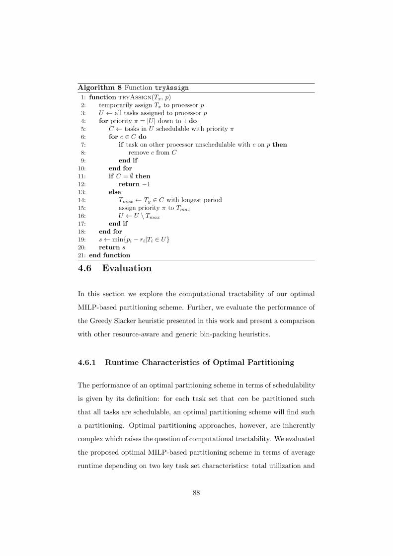
Algorithm 8 Function tryAssign
1: function tryAssign(Tx, p)2: temporarily assign Tx to processor p3: U ← all tasks assigned to processor p4: for priority π = |U | down to 1 do5: C ← tasks in U schedulable with priority π6: for c ∈ C do7: if task on other processor unschedulable with c on p then8: remove c from C9: end if
10: end for11: if C = ∅ then12: return −113: else14: Tmax ← Ty ∈ C with longest period15: assign priority π to Tmax
16: U ← U \ Tmax
17: end if18: end for19: s← minpi − ri|Ti ∈ U20: return s21: end function
4.6 Evaluation
In this section we explore the computational tractability of our optimal
MILP-based partitioning scheme. Further, we evaluate the performance of
the Greedy Slacker heuristic presented in this work and present a comparison
with other resource-aware and generic bin-packing heuristics.
4.6.1 Runtime Characteristics of Optimal Partitioning
The performance of an optimal partitioning scheme in terms of schedulability
is given by its definition: for each task set that can be partitioned such
that all tasks are schedulable, an optimal partitioning scheme will find such
a partitioning. Optimal partitioning approaches, however, are inherently
complex which raises the question of computational tractability. We evaluated
the proposed optimal MILP-based partitioning scheme in terms of average
runtime depending on two key task set characteristics: total utilization and
88

0
1
2
3
4
5
6
7
8
0 0.5 1 1.5 2 2.5 3 3.5 4
avera
ge r
unti
me [
s]
utilization
3 tasks per processor (12 total)4 tasks per processor (16 total)
(a) Average runtimes for MILP solving in seconds while varying total utilization.
0
10
20
30
40
50
60
70
80
4 6 8 10 12 14 16 18 20
avera
ge r
unti
me [
s]
tasks
utilization 2.0utilization 2.5utilization 3.0
(b) Average runtimes for MILP solving in seconds while varying task set size.
Figure 4.2: ILP solving times.
task set size. For solving the generated MILPs, we used the CPLEX 12.4 [2]
optimizer running on a server-class machine equipped with 24 Intel Xeon
X5650 cores with a speed of 2.66 GHz and 48 GB main memory.
In the first experiment, we measured the runtime as the total utilization
of the input task sets increased. Increasing the total utilization limits the
options for a valid partitioning, and hence the partitioning problem gets
harder to solve. For our experiment, we assumed a multicore platform with
m = 4 processors and evaluated task sets with 3 or 4 tasks per processor
while varying the total utilization parameter. For each utilization value, 100
sample task sets were considered. The task periods are chosen at random
89
from [10ms, 100ms] according to a log-uniform distribution. Each task issues
a requests for the single shared resource with a probability of 0.2. In case
the shared resource is accessed, the critical section length is set to 100µs.
The results shown in Figure 4.2a show that the runtime grows as the total
utilization increases and the partitioning problem becomes harder to solve.
Interestingly, the results exhibit a stepwise increase in runtime each time the
total utilization approaches the next-largest integer. Further, the runtime
grows rapidly as the total utilization approaches m since the partitioning
problem becomes (much) harder with decreasing spare capacity.
In our second experiment, we evaluated the impact of task set size on solving
time. An increase in task set size leads to a larger MILP size, and hence
potentially to longer solving times. To study this effect, we fixed the total
task set utilization to 2.0, 2.5 and 3.0, respectively, and varied the number of
tasks in the task set from 4 to 20. Task periods and resource accesses where
chosen as in the first experiment. The results are shown in Figure 4.2b and
exhibit a clear increase in run time as the task set size is growing. Since the
total utilization was kept constant, we ruled out the effect studied in the first
experiment where growing utilization makes the partitioning problem harder
to solve, which is reflected in higher run times. Rather, we attributed the
observed effect to the growth in MILP size (in terms of the number of both
constraints and variables) and resource contention, both of which increase
with each additional task.
The results imply that the increase of total utilization and task set size
each independently cause a significant increase in runtime of the ILP-based
approach presented in Section 4.4. However, the results also demonstrate
that, with today’s hardware, our exact MILP-based partitioning approach
is applicable to small and moderate application instances (note that the
runtimes reported in Figures 4.2a and 4.2b are in the range of a couple of
seconds on average). Even though run times may grow quickly for larger
90
applications, our MILP-based partitioning technique may still be an accept-
able approach as it may well be worth the cost in the context of commercial
development cycles that can stretch many months or even years.
For settings where the computational complexity of the MILP-based approach
is prohibitive, we proposed the resource-aware Greedy Slacker partitioning
heuristics, which we evaluated with schedulability experiments, as we discuss
next.
4.6.2 Partitioning Heuristic Evaluation
For the performance comparison of our Greedy Slacker heuristic with other
partitioning heuristics, we generated task sets with a broad range of con-
figurations. We considered systems with 8 and 16 processors and 1 to 32
resources shared among the tasks. The task sets were generated using the
approach presented by Emberson et al . [68] with periods chosen according to
a log-uniform distribution from either [3ms, 33ms] (short) or [10ms, 100ms]
(moderate). The average per-task utilization was set to either 0.1, 0.2 or
0.3. For each configuration, we choose a resource sharing factor (rsf ) of
either 0.1, 0.25, 0.5 or 0.75, which, for each task and each resource, gives the
probability of the task accessing the resource. For each accessed resource,
only a single request is issued (i.e., Ni,q) with a critical section length chosen
either from [1us, 15us] (short CSLs) or [1us, 100us] (medium CSLs). For
each data point in the presented results, we generated and evaluated 100
sample data sets.
We compared schedulability under the Greedy Slacker heuristic, the MPCP
partitioning heuristic [92], BPA [109], and the resource-oblivious any-fit
heuristic (which tries the first-, best-, next-, and worst-fit strategies, and
returns the result of the first to succeed). For any-fit, we considered the
following variants:
91
• AF-util : plain any-fit heuristic (as summarized in Section 4.2) as a
baseline without a schedulability test;
• AF-RTA: similar to AF-util, but an additional response-time analysis
is performed to rule out assignment decisions that would render a task
set unschedulable immediately; and
• AF-RTA-B : similar to AF-RTA, but the MSRP blocking bounds are
applied, so that the blocking effects due to resource sharing are consid-
ered.
Out of the large number of configurations we evaluated, we present the results
for one exemplary configuration in Figure 4.3a to highlight typical trends.
The results of this configuration resembles trends observable in many of the
configurations considered. With a growing number of tasks in each task
set, both the contention for the shared resources and the total utilization
increases. Up to a task set size of n ≈ 50, AF-RTA-B is able to successfully
produce valid partitionings for all task sets, but schedulability quickly drops
for larger task sets. Surprisingly, AF-RTA and AF-util exhibit virtually
the same schedulability as AF-RTA-B. This is due to the fact that the AF
strategy applies the worst-first heuristic first, which distributes tasks roughly
evenly among all cores. This benefits schedulability such that response-time
and blocking checks are superfluous for most low-utilization task sets. In this
particular scenario, the Greedy Slacker heuristic is able to determine valid
partitionings for all task sets with up to 54 tasks, and overall Greedy Slacker
achieves the highest schedulability among the considered heuristics.
Surprisingly, both the MPCP heuristic and BPA led to significantly lower
schedulability than the AF heuristic. This effect was unexpected since both
the MPCP heuristic and BPA were particularly designed for scenarios with
resource sharing, while AF is resource-oblivious. We found that the reason
for this effect lies in the way BPA and the MPCP heuristic partition task
92
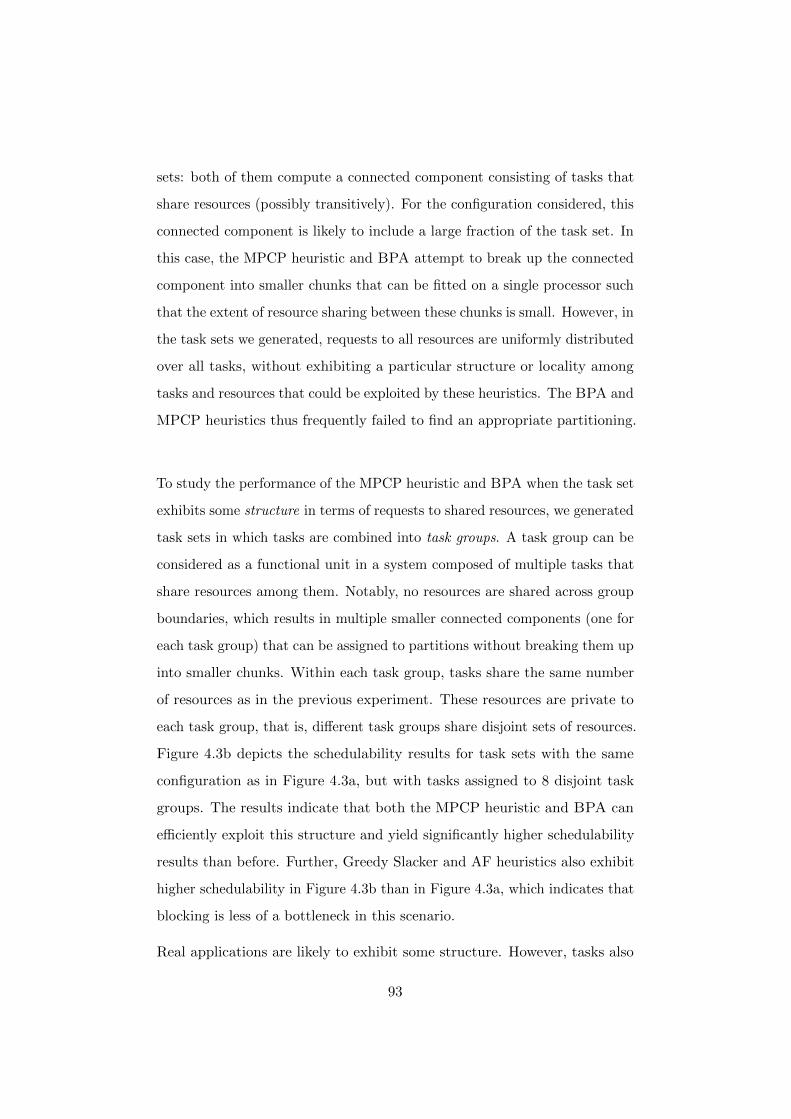
sets: both of them compute a connected component consisting of tasks that
share resources (possibly transitively). For the configuration considered, this
connected component is likely to include a large fraction of the task set. In
this case, the MPCP heuristic and BPA attempt to break up the connected
component into smaller chunks that can be fitted on a single processor such
that the extent of resource sharing between these chunks is small. However, in
the task sets we generated, requests to all resources are uniformly distributed
over all tasks, without exhibiting a particular structure or locality among
tasks and resources that could be exploited by these heuristics. The BPA and
MPCP heuristics thus frequently failed to find an appropriate partitioning.
To study the performance of the MPCP heuristic and BPA when the task set
exhibits some structure in terms of requests to shared resources, we generated
task sets in which tasks are combined into task groups. A task group can be
considered as a functional unit in a system composed of multiple tasks that
share resources among them. Notably, no resources are shared across group
boundaries, which results in multiple smaller connected components (one for
each task group) that can be assigned to partitions without breaking them up
into smaller chunks. Within each task group, tasks share the same number
of resources as in the previous experiment. These resources are private to
each task group, that is, different task groups share disjoint sets of resources.
Figure 4.3b depicts the schedulability results for task sets with the same
configuration as in Figure 4.3a, but with tasks assigned to 8 disjoint task
groups. The results indicate that both the MPCP heuristic and BPA can
efficiently exploit this structure and yield significantly higher schedulability
results than before. Further, Greedy Slacker and AF heuristics also exhibit
higher schedulability in Figure 4.3b than in Figure 4.3a, which indicates that
blocking is less of a bottleneck in this scenario.
Real applications are likely to exhibit some structure. However, tasks also
93
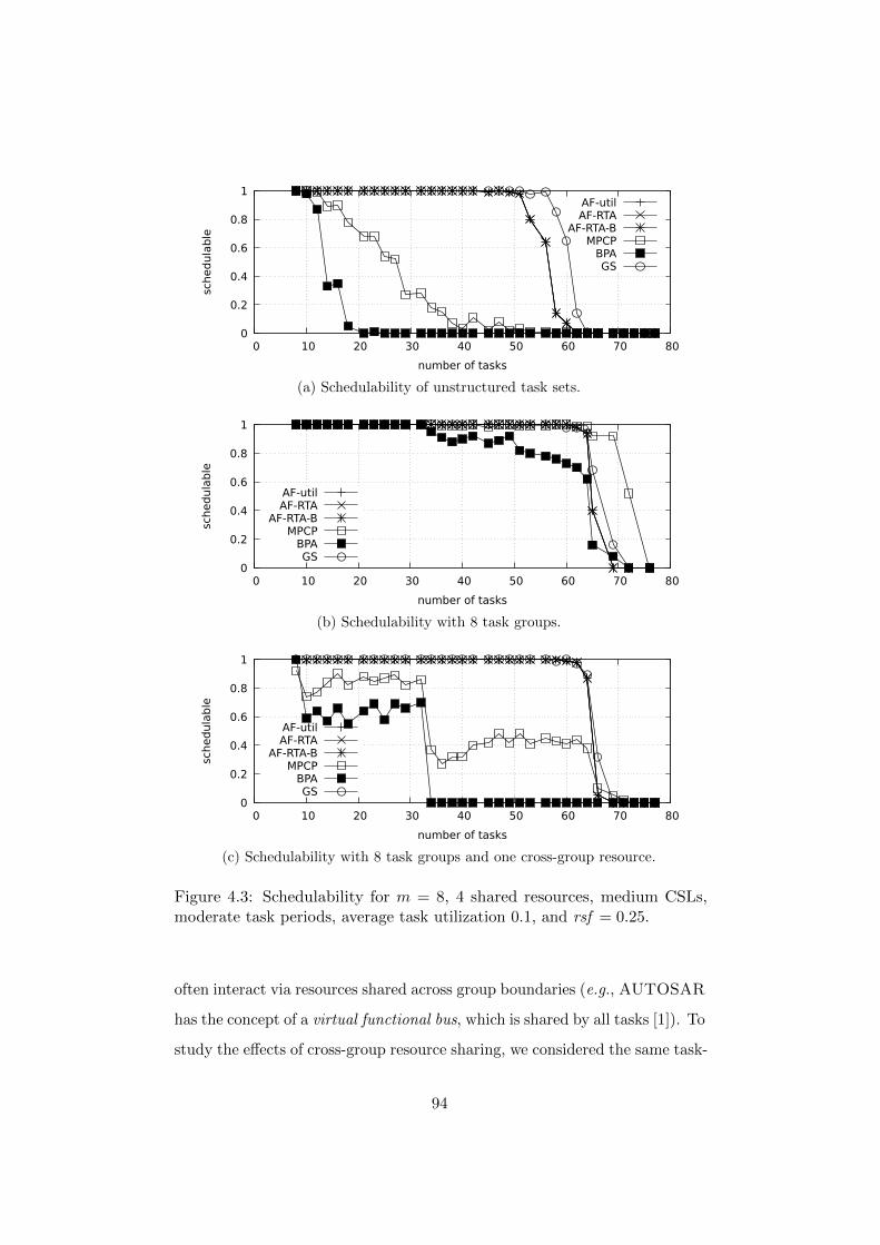
0
0.2
0.4
0.6
0.8
1
0 10 20 30 40 50 60 70 80
sched
ula
ble
number of tasks
AF-utilAF-RTA
AF-RTA-BMPCP
BPAGS
(a) Schedulability of unstructured task sets.
0
0.2
0.4
0.6
0.8
1
0 10 20 30 40 50 60 70 80
sched
ula
ble
number of tasks
AF-utilAF-RTA
AF-RTA-BMPCP
BPAGS
(b) Schedulability with 8 task groups.
0
0.2
0.4
0.6
0.8
1
0 10 20 30 40 50 60 70 80
sched
ula
ble
number of tasks
AF-utilAF-RTA
AF-RTA-BMPCP
BPAGS
(c) Schedulability with 8 task groups and one cross-group resource.
Figure 4.3: Schedulability for m = 8, 4 shared resources, medium CSLs,moderate task periods, average task utilization 0.1, and rsf = 0.25.
often interact via resources shared across group boundaries (e.g., AUTOSAR
has the concept of a virtual functional bus, which is shared by all tasks [1]). To
study the effects of cross-group resource sharing, we considered the same task-
94
group scenario as before with the difference that a single resource is shared
by all task groups. The results are shown in Figure 4.3c. Introducing cross-
group resource sharing again results in a few, large connected components
that the MPCP heuristic and BPA fail to partition effectively. Notably,
the Greedy Slacker heuristic yields high schedulability results independently
of the structure that a task set may (or may not) exhibit, and does not
depend on any protocol-specific heuristics or parameters (besides appropriate
response-time analysis). The reported trends can be observed over the full
range of considered configurations, which shows Greedy Slacker to be an
attractive choice in a variety of scenarios, especially if it cannot be guaranteed
that task sets will always exhibit a convenient structure.
4.7 Summary
In this chapter, we have considered the problem of partitioning a set of
sporadic real-time tasks that share resources protected by the MSRP onto a
set of identical processors. Our work is motivated by the common need to
minimize SWaP requirements and component costs to the extent possible. To
this end, we presented an MILP-based approach for task set partitioning and
priority assignment for shared-memory multiprocessor systems with shared
resources. In contrast to commonly used partitioning heuristics, this approach
yields optimal results (with regard to the underlying schedulability analysis)
and thereby avoids over-provisioning, but is subject to high computational
costs.
For cases where the cost of the MILP-based partitioning approach cannot be
afforded, we presented Greedy Slacker, a novel resource-aware partitioning
heuristic, which we have demonstrated to perform well on average. Greedy
Slacker is generic as it is neither tailored to a specific locking protocol nor
dependent on task-set-specific parameter tuning, and, due to its simplicity,
95

it is resilient in the sense that it is able to exploit locality when existent
without unreasonably degrading in performance if faced with task sets not
exhibiting such patterns, unlike the MPCP heuristic and BPA.
Our MILP-based partitioning scheme encodes Gai et al .’s analysis of the
MSRP [72], and we also employed the same analysis for the MSRP in
combination with the partitioning heuristics we evaluated, including our
Greedy Slacker heuristic. Besides the F|N locks used for global resources as
part of the MSRP, a variety of other types of spin locks have been presented in
prior work. The spin lock types considered in this thesis (see Section 2.4.2 for
an overview) differ in their request ordering policy and whether preemptions
while spinning are allowed, and it is unclear which of these types (if any)
generally ensures minimal blocking. To that end, in the next chapter, we
present the results of a qualitative comparison between the different spin
lock types considered in this thesis.
96
Chapter 5
Qualitative Comparison of
Spin Lock Types
5.1 Introduction
In the previous chapter, we presented methods for efficiently partitioning
task sets sharing resources protected by the MSRP, that is, the SRP for local
and F|N locks for global resources. As overviewed in Table 2.1 (Section 2.4.2),
spin locks with ordering policies other than FIFO and spin locks allowing
preemptions while spinning have been presented. In this chapter, we conduct
a qualitative comparison between preemptable and non-preemptable spin
locks, and the different ordering policies. In particular, we investigate the
following two questions:
Q1: Is there an ordering policy that always results in minimal blocking?
Q2: Does preemptable or non-preemptable spinning result in minimal block-
ing?
We seek to answer these questions by comparing the different spin lock types
97
at an abstract level, focusing on their properties independent of concrete task
sets. For comparing the spin lock types, we establish a dominance relation
between them.
5.2 Dominance of Spin Lock Types
Intuitively, a spin lock type dominates another one if it never performs worse.
More formally, we define the dominance relation between spin lock types as
follows.
Def. 1: Dominance of spin lock types. Spin locks of type A dominate
spin locks of type B if and only if for any task set and for each task therein,
the worst-case blocking duration under A does not exceed the worst-case
blocking duration under B.
Here we choose to define the dominance relation in terms of the actual worst-
case blocking duration instead of blocking bounds or task response times
(and hence timeliness). The reason is that focusing on the worst-case blocking
duration enables us to exclude potentially confounding factors such as the
response-time analysis and the blocking analysis that may yield non-tight
bounds. In fact, the dominance relations established here do not necessarily
hold for blocking bounds that cannot be guaranteed to be tight.
Note that the above dominance relation is transitive, which directly follows
from the transitivity of the “does not exceed” (or ≤) relation. Dominance, as
defined above, does not establish a total order among spin lock types, as some
types are incomparable. We formally define incomparability as follows.
Def. 2: Incomparability of spin lock types. The spin lock types A and
B are incomparable if and only if A does not dominate B, and B does not
dominate A.
98
As we show next, preemptable and non-preemptable spin locks are generally
incomparable, regardless of their request ordering policy.
5.3 Non-Preemptable and Preemptable Spin Locks
are Incomparable
We show that each non-preemptable spin lock is incomparable to all preempt-
able spin locks by showing that dominance between them is impossible.
Lemma 2. No *|N lock dominates any *|P lock.
Proof. Consider the schedule depicted in Figure 5.1 for any *|N lock in which
jobs of Ti can only incur arrival blocking, and no other forms of blocking (since
Ti does not access any shared resources and Ti is the highest-priority task on
its processor). Throughout the interval [0, 5), the first job of Ti, Ji, incurs
arrival blocking: during the interval [0, 4), job Jl spins non-preemptably while
waiting to acquired the lock held by Jx. Hence, Ji is transitively blocked by
the remote request issued by Jx. During the interval [4, 5), job Jl executes
its critical section non-preemptably, and hence causes Ji to incur further
blocking. In total, Ji is blocked for bi = 5 time units.
Under any *|P lock, requests issued by tasks on remote processors cannot
contribute to arrival blocking, and hence, only Jl’s request can cause Ti’s
jobs to incur arrival blocking. Each of Ti’s jobs can incur arrival blocking
due to at most request issued by a local lower-priority task and hence, Ti’s
blocking duration is bounded by the critical section length of Tl’s request.
That is, bi = 1.
Since Ji is blocked for bi = 5 time units in the schedule depicted in Figure 5.1
under any *|N lock while Ji can be blocked for only bi = 1 time units in the
worst-case under any *|P lock, no *|N lock can dominate any *|P lock.
99

50 10
Ti
Tx
`1
P2
15
P1
Tl
`1
job executing
job spinning while waiting for resource
job executingcritical section
job holding resource `1`1
job release
Figure 5.1: Example schedule for non-preemptable spin locks.
Note that the above lemma (and its proof) is oblivious to the ordering
guarantees that a spin lock may enforce, and hence applies to any request
ordering policy.
The reverse of the previous lemma holds as well, as we show in the follow-
ing.
Lemma 3. No *|P lock dominates any *|N lock.
Proof. Consider the schedule depicted in Figure 5.2 for any *|P lock. Through-
out the interval [0, 9), job Ji is either busy waiting to acquire the lock, or
preempted by higher-priority jobs. In total, Ji is blocked for bi = 4 time
units. While busy waiting, jobs of the higher-priority tasks Th and Tk repeat-
edly preempt Ji. These preemptions cause Ji’s request to be cancelled and
re-issued as Ji resumes (see Section 2.4.2). Each of Ji’s re-issued requests
conflicts with a request issued by a job of Tx at the same time, and the
requests issued by jobs of Tx are served instead of Ji’s request.
Under any *|N lock, Ji cannot be preempted by higher-priority jobs while
busy-waiting, and hence, Ji’s request cannot be cancelled. Besides Ji, only
Tx’s jobs accesses the lock. Since Tx has a period of px = 2 and a critical
section length of Lx = 1, Ji’s request is blocked for at most one time unit
100
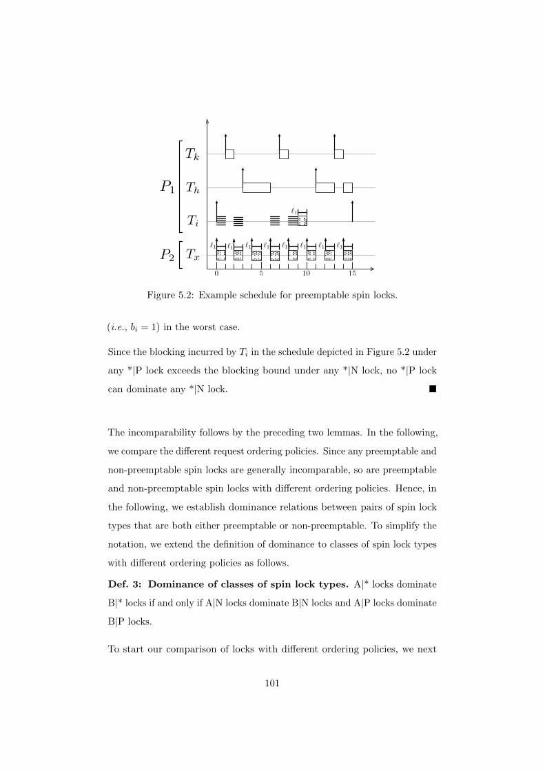
50 10
Th
Tx
`1
P2
15
P1
Ti
Tk
`1 `1 `1 `1 `1 `1 `1 `1
Figure 5.2: Example schedule for preemptable spin locks.
(i.e., bi = 1) in the worst case.
Since the blocking incurred by Ti in the schedule depicted in Figure 5.2 under
any *|P lock exceeds the blocking bound under any *|N lock, no *|P lock
can dominate any *|N lock.
The incomparability follows by the preceding two lemmas. In the following,
we compare the different request ordering policies. Since any preemptable and
non-preemptable spin locks are generally incomparable, so are preemptable
and non-preemptable spin locks with different ordering policies. Hence, in
the following, we establish dominance relations between pairs of spin lock
types that are both either preemptable or non-preemptable. To simplify the
notation, we extend the definition of dominance to classes of spin lock types
with different ordering policies as follows.
Def. 3: Dominance of classes of spin lock types. A|* locks dominate
B|* locks if and only if A|N locks dominate B|N locks and A|P locks dominate
B|P locks.
To start our comparison of locks with different ordering policies, we next
101
show that both priority-ordering and FIFO-ordering are “strong” guarantees
in the sense that spin locks using them dominate unordered spin locks.
5.4 F|* and P|* Locks Dominate U|* Locks
In the following, we show that FIFO- and priority-ordered spin locks dominate
unordered locks, and then we show that the reverse does not hold.
Lemma 4. F|* and P|* locks dominate U|* locks.
Proof. Consider an arbitrary task Ti from an arbitrary task set sharing
resources protected by F|* or P|* locks. Let S denote a schedule under which
Ji, a job of Ti, incurs the worst-case blocking duration. Since, by definition,
U|* locks are not required to serve requests in any particular order, they may
serve requests in FIFO- or priority-order. Hence, if U|* locks are used instead
of F|* or P|* locks to protect the shared resources, schedule S is possible and
valid under U|* locks as well. Then Ji can incur the same blocking duration
under U|* locks.
Note that, in case of P|* locks, the above argument holds for any priority
assignment, even when all requests are issued with the same priority (in
which case P|* locks do not give any guarantees on the ordering, similar to
U|* locks). The above lemma shows that the worst-case blocking incurred
under U|* locks is at least the worst-case blocking possible with F|* and P|*
locks, and hence, the worst-case blocking duration under U|* locks can never
be lower. To show the strict dominance, we next show that the blocking
under U|* locks can also lead to longer blocking compared to F|* and P|*
locks.
Lemma 5. U|* locks dominate neither F|* nor P|* locks.
Proof. Consider the schedule depicted in Figure 5.3 for U|* locks in which
102

50 10
Ti
Ty
`1
P3
15
P1
Tx
`1
`1`1
P2
Figure 5.3: Example schedule for unordered spin locks.
Ji’s request is blocked for bi = 4 time units. Note that, in this schedule, both
of Jx’s requests are served before Ji’s request, and Ji’s request was issued
before Jx’s second request. Further, note that at most one task is assigned
to each processor, rendering preemptions impossible.
Under F|* locks, since requests are served in FIFO-order and preemptions
while spinning are impossible, each request can be blocked by at most one
request for the same resource from each other processor. Hence, Ji’s request
can be blocked by at most one of Jx’s request and one of Jy’s request. As a
result, Ji’s blocking duration is bounded by bi = 3 time units.
Under P|* locks, each request can be blocked by at most one remote request
issued with lower priority. Consider a priority assignment in which Ji’s
request is assigned a priority higher than the priority assigned to both of Jx’s
requests and Jy’s request. Then Ji’s request can be blocked by either one of
Jx’s requests or Jy’s request. Hence, Ji’s blocking duration is bounded by
bi = 2 time units (the length of Jy’s request, which is the longest one).
The blocking incurred by Ji under U|* locks in the schedule depicted in
Figure 5.3 exceeds Ti’s blocking bound of bi = 3 for F|* locks and bi = 2 for
P|* locks, respectively. Hence, U|* locks can dominate neither F|* nor P|*
locks.
103
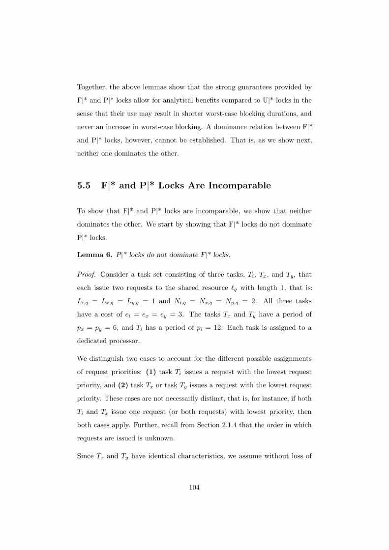
Together, the above lemmas show that the strong guarantees provided by
F|* and P|* locks allow for analytical benefits compared to U|* locks in the
sense that their use may result in shorter worst-case blocking durations, and
never an increase in worst-case blocking. A dominance relation between F|*
and P|* locks, however, cannot be established. That is, as we show next,
neither one dominates the other.
5.5 F|* and P|* Locks Are Incomparable
To show that F|* and P|* locks are incomparable, we show that neither
dominates the other. We start by showing that F|* locks do not dominate
P|* locks.
Lemma 6. P|* locks do not dominate F|* locks.
Proof. Consider a task set consisting of three tasks, Ti, Tx, and Ty, that
each issue two requests to the shared resource `q with length 1, that is:
Li,q = Lx,q = Ly,q = 1 and Ni,q = Nx,q = Ny,q = 2. All three tasks
have a cost of ei = ex = ey = 3. The tasks Tx and Ty have a period of
px = py = 6, and Ti has a period of pi = 12. Each task is assigned to a
dedicated processor.
We distinguish two cases to account for the different possible assignments
of request priorities: (1) task Ti issues a request with the lowest request
priority, and (2) task Tx or task Ty issues a request with the lowest request
priority. These cases are not necessarily distinct, that is, for instance, if both
Ti and Tx issue one request (or both requests) with lowest priority, then
both cases apply. Further, recall from Section 2.1.4 that the order in which
requests are issued is unknown.
Since Tx and Ty have identical characteristics, we assume without loss of
104
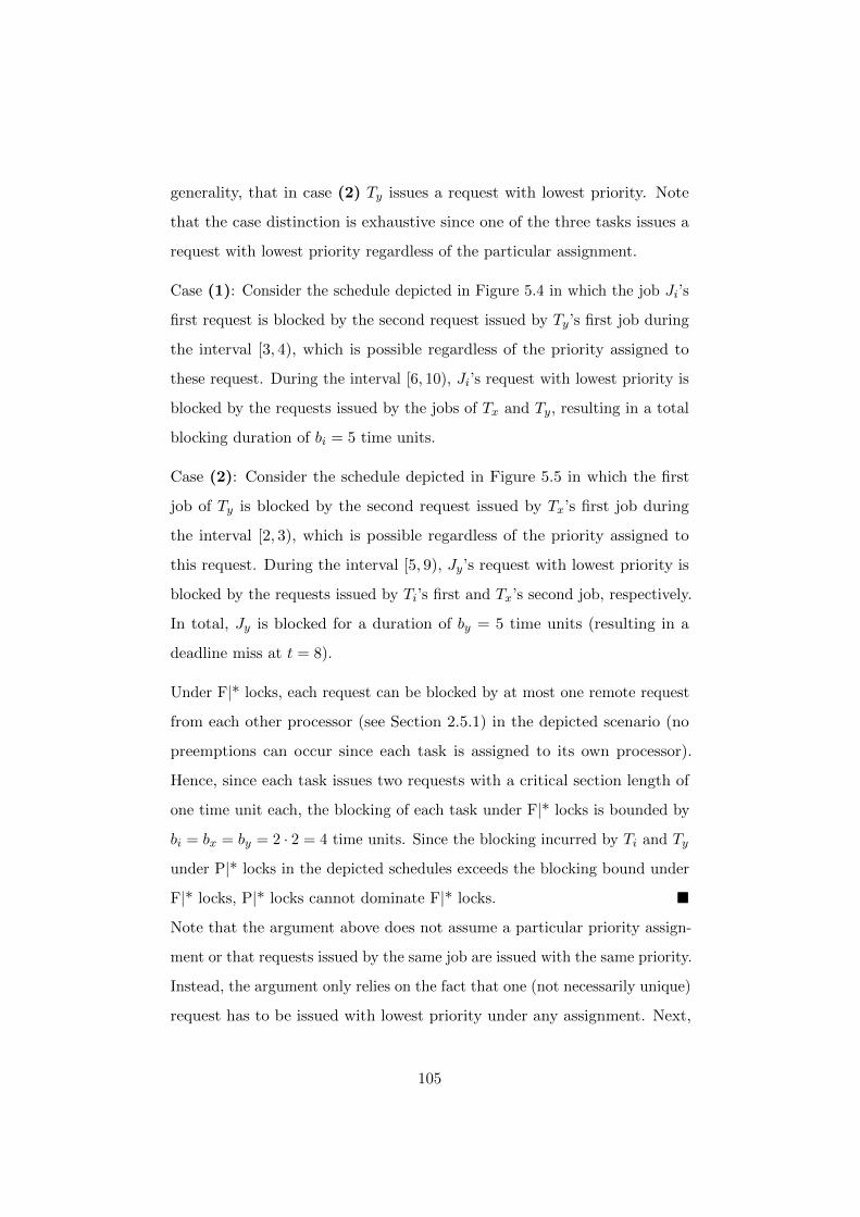
generality, that in case (2) Ty issues a request with lowest priority. Note
that the case distinction is exhaustive since one of the three tasks issues a
request with lowest priority regardless of the particular assignment.
Case (1): Consider the schedule depicted in Figure 5.4 in which the job Ji’s
first request is blocked by the second request issued by Ty’s first job during
the interval [3, 4), which is possible regardless of the priority assigned to
these request. During the interval [6, 10), Ji’s request with lowest priority is
blocked by the requests issued by the jobs of Tx and Ty, resulting in a total
blocking duration of bi = 5 time units.
Case (2): Consider the schedule depicted in Figure 5.5 in which the first
job of Ty is blocked by the second request issued by Tx’s first job during
the interval [2, 3), which is possible regardless of the priority assigned to
this request. During the interval [5, 9), Jy’s request with lowest priority is
blocked by the requests issued by Ti’s first and Tx’s second job, respectively.
In total, Jy is blocked for a duration of by = 5 time units (resulting in a
deadline miss at t = 8).
Under F|* locks, each request can be blocked by at most one remote request
from each other processor (see Section 2.5.1) in the depicted scenario (no
preemptions can occur since each task is assigned to its own processor).
Hence, since each task issues two requests with a critical section length of
one time unit each, the blocking of each task under F|* locks is bounded by
bi = bx = by = 2 · 2 = 4 time units. Since the blocking incurred by Ti and Ty
under P|* locks in the depicted schedules exceeds the blocking bound under
F|* locks, P|* locks cannot dominate F|* locks.
Note that the argument above does not assume a particular priority assign-
ment or that requests issued by the same job are issued with the same priority.
Instead, the argument only relies on the fact that one (not necessarily unique)
request has to be issued with lowest priority under any assignment. Next,
105
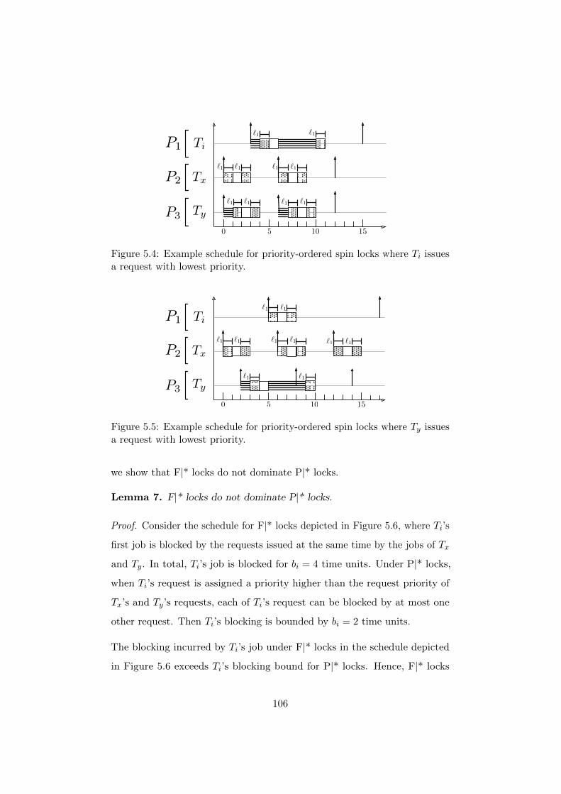
50 10
Ti
Ty
`1
P3
15
P1
Tx
`1`1
P2
`1
`1`1
`1 `1`1`1
Figure 5.4: Example schedule for priority-ordered spin locks where Ti issuesa request with lowest priority.
50 10
Ti
TyP3
15
P1
Tx
`1
`1`1
P2
`1`1
`1
`1`1
`1`1
Figure 5.5: Example schedule for priority-ordered spin locks where Ty issuesa request with lowest priority.
we show that F|* locks do not dominate P|* locks.
Lemma 7. F|* locks do not dominate P|* locks.
Proof. Consider the schedule for F|* locks depicted in Figure 5.6, where Ti’s
first job is blocked by the requests issued at the same time by the jobs of Tx
and Ty. In total, Ti’s job is blocked for bi = 4 time units. Under P|* locks,
when Ti’s request is assigned a priority higher than the request priority of
Tx’s and Ty’s requests, each of Ti’s request can be blocked by at most one
other request. Then Ti’s blocking is bounded by bi = 2 time units.
The blocking incurred by Ti’s job under F|* locks in the schedule depicted
in Figure 5.6 exceeds Ti’s blocking bound for P|* locks. Hence, F|* locks
106
50 10
Ti
TyP3
P1
Tx
`1
`1
P2
`1
Figure 5.6: Example schedule for FIFO-ordered spin locks.
cannot dominate P|* locks.
Together, the above two lemmas show that F|* and P|* locks are incompara-
ble.
5.6 PF|* Locks Dominate both F|* and P|* Locks
While F|* and P|* locks are incomparable, as shown above, priority-ordered
spin locks with FIFO tie-breaking, PF|* locks, dominate both of them. The
underlying reason is that PF|* locks integrate both mechanisms, and with
an appropriate assignment of priorities, PF|* locks can behave identically to
F|* or P|* locks, and hence PF|* locks dominate both of them. The reverse,
however, is not true: neither F|* nor P|* locks dominate PF|* locks.
Lemma 8. PF|* locks dominate P|* and F|* locks.
Proof. Follows from the preceding discussion.
Lemma 9. Neither F|* nor P|* locks dominate PF|* locks.
Proof. Follows from Lemmas 6 and 7 and the transitivity of the dominance
relation.
107

PF|N
F|N P|N
U|N
A B A dominates B A B A and B are incomparable
PF|P
F|P P|P
U|P
Figure 5.7: Summary of dominance and incomparability results.
5.7 Summary
We summarize the results of our qualitative comparison in Figure 5.7. Both
F|* and P|* locks result in less worst-case blocking than U|* locks. This
finding roughly matches the intuition that some meaningful ordering pol-
icy (FIFO or priority) should yield better results than no ordering policy
(unordered). F|* and P|* locks are incomparable, which indicates that the
impact of these policies cannot be stated in general terms, but rather de-
pends on concrete task sets. F|* and P|* locks are dominated by PF|* locks,
comprising mechanisms for both FIFO- and priority-ordering.
A perhaps surprising finding is that preemptable and non-preemptable spin
locks are generally incomparable, regardless of the ordering policy. This
result holds even for spin lock types with different ordering policies, e.g.,
FP|N and U|P are incomparable, although FP|N dominate U|N locks and
FP|P dominate U|P.
The results of our qualitative comparison show that strong ordering guaran-
tees have clear benefits over unordered spin locks — a not entirely unexpected
outcome. At the same time, we have shown FIFO- and priority-ordered as
well as preemptable and non-preemptable spin locks to be incomparable.
108
Although these results may be considered unsatisfactory as no “lock type
to rule them all” could be identified, they justify the availability of these
various types of spin locks to support a broad range of different applications.
Incomparability also implies that the effect of the spin lock type on the
blocking duration depends on concrete task sets. In the next chapter, we
present a fine-grained blocking analysis approach to derive blocking bounds
for concrete task sets under the various spin lock types considered.
109

Chapter 6
Analysis of Non-Nested Spin
Locks1
6.1 Introduction
In this chapter we present a novel approach for fine-grained blocking analysis
of non-nested spin locks. Our motivation is twofold: first, out of the spin
lock types we consider in this thesis (see Table 2.1 in Section 2.4.2 for an
overview), only for F|N locks a fine-grained blocking analysis is available
(as part of the MSRP analysis). The lack of a blocking analysis renders
the other spin lock types unusable for real-time workloads. Second, even
though analyses of the MSRP are available in prior work, they are inherently
pessimistic. Pessimistic blocking bounds can result in a waste of resources,
which is particularly undesirable for embedded real-time applications often
developed under SWaP (space, weight and power) constraints. With our
blocking analysis approach we aim to eliminate the pessimism inherent in
prior analyses and support a range of spin lock types for which no prior
1This chapter is based on [133].
110
analysis is available. Before detailing our blocking analysis, we describe why
prior analyses are pessimistic.
6.2 Pessimism in Prior Analyses for Spin Locks
In this section, we illustrate the pessimism inherent in prior blocking analyses
for spin locks.
6.2.1 Classic MSRP
The classic analysis of the MSRP (summarized in Section 2.5.1) bounds
the blocking that each individual request incurs, which can lead to double-
counting of conflicting requests when the task under analysis issues multiple
requests for the same resource. We demonstrate this effect with an exam-
ple.
Consider a two tasks, Ti and Tx, assigned to different processors. The periods
of the tasks are pi = 6 and px = 17, and execution costs are ei = 3 and
ex = 7. Both tasks access the shared resource `q; each job of Ti issues
Ni,q = 2 requests of length Li,q = 1 and each job of Tx issues one request of
length Lx,q = 2. Figure 6.1 depicts a schedule for these two tasks in which
Ti’s first job, Ji,1, is blocked by Tx’s job holding `q during the time interval
[0, 2). At time t = 2, Ji,1 acquires the lock and executes the critical section.
Ji,1’s second request issued at time t = 4 is executed immediately as `q is
not held at that time. Ji,1 finishes before deadline at t = 5.
Applying the classic MSRP blocking analysis to Ti in this example is straight-
forward: local and non-preemptive blocking cannot occur since no other task
is assigned to Ti’s processor. Hence, βloci = βNPi = 0. However, as shown in
the depicted schedule, Ti can incur remote blocking that has to be accounted
111
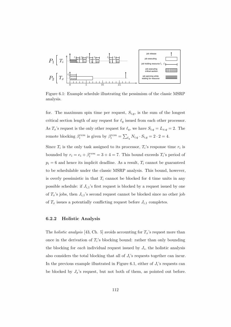
50 10
Ti
Tx
`1 job executing
job executingcritical section
job holding resource `1`1
job release
`1 job spinning while waiting for resourceP2
15
`1 `1 `1 `1 `1
P1
Figure 6.1: Example schedule illustrating the pessimism of the classic MSRPanalysis.
for. The maximum spin time per request, Si,q, is the sum of the longest
critical section length of any request for `q issued from each other processor.
As Tx’s request is the only other request for `q, we have Si,q = Lx,q = 2. The
remote blocking βremi is given by βremi =∑
`qNi,q · Si,q = 2 · 2 = 4.
Since Ti is the only task assigned to its processor, Ti’s response time ri is
bounded by ri = ei + βremi = 3 + 4 = 7. This bound exceeds Ti’s period of
pi = 6 and hence its implicit deadline. As a result, Ti cannot be guaranteed
to be schedulable under the classic MSRP analysis. This bound, however,
is overly pessimistic in that Ti cannot be blocked for 4 time units in any
possible schedule: if Ji,1’s first request is blocked by a request issued by one
of Tx’s jobs, then Ji,1’s second request cannot be blocked since no other job
of Tx issues a potentially conflicting request before Ji,1 completes.
6.2.2 Holistic Analysis
The holistic analysis [43, Ch. 5] avoids accounting for Tx’s request more than
once in the derivation of Ti’s blocking bound: rather than only bounding
the blocking for each individual request issued by Ji, the holistic analysis
also considers the total blocking that all of Ji’s requests together can incur.
In the previous example illustrated in Figure 6.1, either of Ji’s requests can
be blocked by Jx’s request, but not both of them, as pointed out before.
112
Based on this observation, the holistic analysis accounts only once for Jx’s
request (as it can block at most one of Ji’s requests), which reduces the
pessimism of the blocking bounds compared with the classic MSRP analysis.
In the example above, the holistic analysis bounds Ti’s blocking to bi = 2
time units instead of four. This less pessimistic blocking bound results in a
response-time bound of ri = 5, and hence, Ti can be guaranteed to meet its
timing requirements.
The holistic analysis, similar to the classic MSRP analysis, relies on execution
time inflation. That is, in the schedulability analysis the inflated execution
time e′i = ei + bi is used to account for a blocking bound bi. This approach,
however, is inherently pessimistic. To illustrate this pessimism, we consider
an example with one additional task. The two tasks from the previous
example are defined as before, with the exception that task Ti from the
previous example is now denoted as Th. The additional task, Ti, has a period
of pi = 11 and an execution cost of ei = 2. Task Ti is assigned to Th’s
processor and has a lower scheduling priority, that is, i > h. Figure 6.2
depicts a schedule for this task set in which Ti’s job is preempted throughout
the time intervals [0, 5) and [6, 9).
Note that Ti does not access any shared resources. Yet, Ti incurs transitive
blocking during the interval [0, 2) since Th’s higher-priority job spins while
being blocked by Tx’s request. To illustrate the pessimism due to execution
time inflation in this example, we apply response-time analysis for Ti. As
Ti does not access any shared resources and execution times are inflated
to account for blocking effects, the regular response-time analysis for P-FP
(Equation (2.1)) can be applied:
ri = ei +∑πh<πi
P (Ti)=P (Th)
⌈riph
⌉· e′h.
113
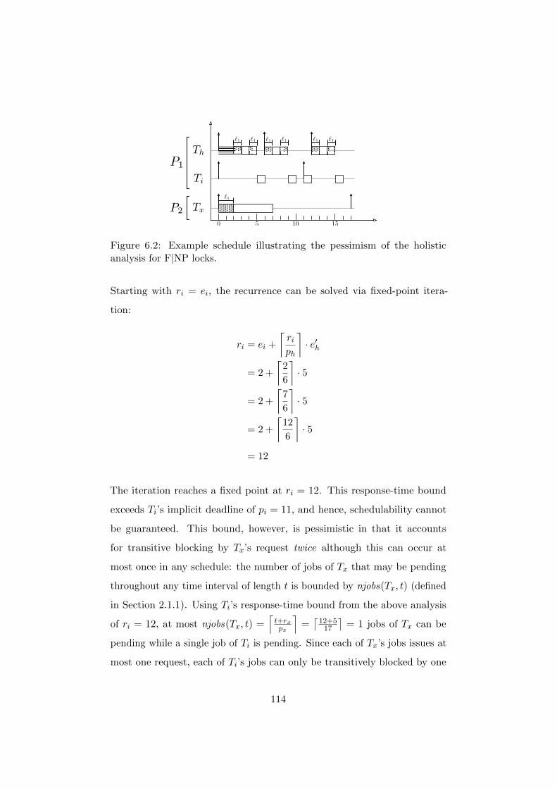
50 10
Th
Tx
`1
`1
P2
15
`1 `1 `1 `1 `1
P1
Ti
Figure 6.2: Example schedule illustrating the pessimism of the holisticanalysis for F|NP locks.
Starting with ri = ei, the recurrence can be solved via fixed-point itera-
tion:
ri = ei +
⌈riph
⌉· e′h
= 2 +
⌈2
6
⌉· 5
= 2 +
⌈7
6
⌉· 5
= 2 +
⌈12
6
⌉· 5
= 12
The iteration reaches a fixed point at ri = 12. This response-time bound
exceeds Ti’s implicit deadline of pi = 11, and hence, schedulability cannot
be guaranteed. This bound, however, is pessimistic in that it accounts
for transitive blocking by Tx’s request twice although this can occur at
most once in any schedule: the number of jobs of Tx that may be pending
throughout any time interval of length t is bounded by njobs(Tx, t) (defined
in Section 2.1.1). Using Ti’s response-time bound from the above analysis
of ri = 12, at most njobs(Tx, t) =⌈t+rxpx
⌉=⌈
12+517
⌉= 1 jobs of Tx can be
pending while a single job of Ti is pending. Since each of Tx’s jobs issues at
most one request, each of Ti’s jobs can only be transitively blocked by one
114
request while the analysis accounts for two blocking request.
The pessimism in the analysis is not specific to the holistic blocking analysis
but rather the technique of execution time inflation. In fact, as we show
next, any analysis based on inflating execution times to account for blocking
effects is inherently pessimistic.
6.2.3 Inherent Pessimism in Execution Time Inflation
In the previous example and the schedule depicted in Figure 6.2, Ti’s first
job is preempted twice by jobs of the higher-priority task Th. The pessimism
in the analysis stems from the fact that the inflation of Th’s execution cost
is accounted for each time one of Th’s jobs is released, that is, dri/phe = 2
times in Ti’s response time, although Ti’s job can incur transitive blocking
at most once. In general, the analysis pessimism grows as the number of
local higher-priority tasks (that can preempt Ti’s job and hence cause Ti’s
job to incur transitive blocking) in the system and the ratio dri/phe (i.e., the
maximum number of jobs released while one of Ti’s job is pending) increase.
Recall that we defined φ to be ratio of shortest and longest period of the
tasks in the system. We state the inherent pessimism of execution time
inflation with the following theorem.
Theorem 3. Any blocking analysis relying on the inflation of job execution
costs can be pessimistic by a factor of Ω(φ · n).
Proof. Let α denote a given, arbitrary non-negative integer parameter. We
construct a scenario in which Ω(n · α) delay is accounted for, actual blocking
is O(1), and where φ = α.
Consider a system consisting of two processors, P1 and P2, a single shared
resource `1, and a task set consisting of n ≥ 3 tasks. The tasks T1, . . . , Tn−2
are assigned to P1 and have parameters pi = 2n− 3 and ei = 1, and access
115

`1 once per job with a negligible critical section length of Li,1 = ε > 0. Task
Tn−1 is assigned to P2 and has parameters pn−1 = α · (2n− 3) and en−1 = 1,
and requests `1 once per job with Ln−1,1 = 1. Finally, the lowest-priority
task Tn with pn = α · (2n − 3) and en = α is assigned to P1 and does not
access `1.
Let rinfn denote Tn’s response-time bound obtained by inflating execution
costs. We have rinfn = en +
∑n−2h=1
⌈rinfnph
⌉e′h, where e′h denotes the inflated
execution time of Th. Since each Th ∈ T1, . . . , Tn−2 directly conflicts with
Tn−1 via `1, we have e′h ≥ eh +Ln−1,1 = eh + 1 under any (mutual exclusion)
locking protocol. Suppose e′h = eh + 1 = 2. Then setting rinfn = α · (2n− 3)
yields a fixed point:
rinfn = α+
n−2∑h=1
⌈rinfn
2n− 3
⌉· 2
= α+n−2∑h=1
⌈α · (2n− 3)
2n− 3
⌉· 2
= α+
n−2∑h=1
α · 2
= α+ (n− 2) · α · 2
= α+ (2n− 4) · α
= α · (2n− 3).
Observe that Tn−1 issues only a single request for `1, and hence T1, . . . , Tn−2
are blocked by at most one request in total while a job Jn is pending. The
actual remote blocking that contributes to Tn’s response time (i.e., the time
that any job on processor P1 spins while Jn is pending) is hence limited to
Ln−1,1 = 1. Hence we have rrealn = en+Ln−1,1 +∑n−2
h=1
⌈rrealnph
⌉·eh, and, since
rrealn ≤ rinfn , also rrealn ≤ en + Ln−1,1 +
∑n−2h=1
⌈rinfnph
⌉· eh.
The pessimism due to execution cost inflation is given by the difference of
116
rrealn and rinfn , where
rinfn − rreal
n ≥ en +
n−2∑h=1
⌈rinfn
ph
⌉(eh + 1)−
(en + Ln−1,1 +
n−2∑h=1
⌈rinfn
ph
⌉· eh
)
=n−2∑h=1
⌈rinfn
ph
⌉− Ln−1,1
=n−2∑h=1
⌈α · (2n− 3)
(2n− 3)
⌉− 1
= (n− 2) · α− 1
= Ω(n · α).
Since φ = α and because actual blocking is limited to Ln−1,1 = O(1), this
establishes that rinfn overestimates the impact of blocking by a factor of
Ω(φ · n).
We illustrate this construction in Figure 6.3 for n = 5 and α = 2. In this
schedule, each job of the tasks T1, T2 and T3 is inflated by 1 time unit to
account for blocking due to T4’s request for `1: e′1 = e′2 = e′3 = 1 + 1 = 2. In
Figure 6.3, T4’s semi-transparent requests are not actually issued by T4, but
still accounted for by the analysis based on execution-time inflation. Applying
response-time analysis for (Equation (2.1)) T5 with inflated execution times
yields a fixed-point with rinfn = 14:
rinf5 = α+
n−2∑h=1
⌈rinfn
2n− 3
⌉· e′h
= 2 +3∑
h=1
⌈14
7
⌉· 2
= 2 +
3∑h=1
2 · 2
= 14.
117

50 10
P1
T1
T2
T3
T4
T5
15 20
P2
`1 `1 `1 `1 `1 `1
`1
`1
`1
`1
`1
`1
Figure 6.3: Schedule illustration the construction from Theorem 3 for α = 2and n = 5. Note that T4’s semi-transparent requests in this schedule (e.g.,at time 4) are not actually issued by T4, but accounted for in the inflatedexecution time of T1, T2 and T3.
This response-time bound accounts for 6 time units of blocking, even though
Ti can be blocked for at most one time unit. First, observe that throughout
any time window of length 6, jobs of T4 issue at most one request for `1, and
hence, during that time at most one request can block T5. Without execution
time inflation, T5’s response time is bounded by 6 time units:
rreal5 = α+ b5 +
n−2∑h=1
⌈rrealn
2n− 3
⌉· eh
= 2 + 1 +
3∑h=1
⌈6
7
⌉· 1
= 3 +3∑
h=1
1 · 1
= 6,
where b5 denotes the blocking that T5 can incur (one of T4’s requests with
length 1). Note that in the response-time analysis above, T5’s blocking is
explicitly accounted for by b5 rather inflated execution times. Next, we
118
introduce a novel blocking analysis approach that similarly does not rely
on execution time inflation and eliminates the pessimism inherent in this
technique.
6.3 A MILP-Based Blocking Analysis Framework
for Spin Locks
Our analysis approach substantially differs from prior blocking analysis
techniques for spin locks. Whereas prior techniques aim to identify or (over-)
approximate the blocking in a worst-case scenario (e.g., [43, Ch. 5] and [72]),
we approach the problem from the opposite direction: we derive invariants
that must hold in any possible schedule based on the properties of the task
set and the type of spin lock to rule out impossible scenarios (similar to [36]),
rather than arguing about the worst case. Among the scenarios not explicitly
ruled out, one with maximum blocking duration is identified.
This method bears several advantages over prior techniques. First, deriving
these invariants that must hold in any possible schedule is easier than directly
bounding the worst case. Each invariant can be proven individually, and
often invariants can be directly inferred from properties of the spin lock type.
Second, these invariants are modular in the sense that they can be freely
combined and re-used for the analysis of different spin lock types that share
some of their properties. Third, in our approach all potentially conflicting
requests are initially assumed to contribute to the blocking duration unless
explicitly ruled out by these invariants. As a result, employing the analysis
without any such invariants or omitting some of them yields safe (albeit
pessimistic) blocking bounds. Conversely, additional invariants can be added
to the existing ones to further improve the analysis, express application-
specific properties, or support different types of spin locks.
119

Our analysis approach is based on Mixed Integer Linear Programming: we
frame the blocking analysis problem as a Mixed Integer Linear Program
(MILP), where the invariants are constraints and the objective is to maximize
the blocking duration. That is, the optimization goal is to find the maximal
blocking among the scenarios not ruled out by the invariants that must
hold in any possible schedule. In the following, we present this approach in
detail.
Types of Blocking under Spin Locks
A job may incur blocking for different causes, and for our analysis we
distinguish two basic forms of blocking: spin delay and arrival blocking.
A request Rx,q,v causes a job Ji to incur spin delay at a time t if either
• (S1) Ji is spinning while waiting to acquire the spin lock on `q at time
t and Rx,q,v is executing at time t (in Figure 2.3, J3’s request causes
J2 to incur spin delay during the interval [1, 4)), or
• (S2) there is a local higher-priority job Jh with P (Ti) = P (Th)∧ h < i
that is spinning while waiting to acquire the spin lock on `q at time t
and Rx,q,v is executing at time t (in Figure 2.3, J4’s request causes J2
to incur spin delay during the interval [8, 9)).
A request Rx,q,v causes a job Ji to incur arrival blocking at a time t if there
is a local lower-priority job Jl with P (Ti) = P (Th) ∧ l > i that either
• (A1) executes the request Rx,q,v at time t (in Figure 2.3, the execution
of J2’s request causes J1 to arrival blocking during the interval [4, 7)),
or spins non-preemptably while waiting to acquire the spin lock on
`q at time t and Rx,q,v is executing at time t (in Figure 2.3, J2 spins
non-preemptably while waiting for J3 to release `1 during the interval
[3, 4), hence, J3’s request causes J1 to incur arrival blocking during the
120

interval [3, 4)), or
• (A2) executes Rx,q,v, `q is a local resource, and `q has a priority ceiling
higher or equal to Ti’s priority (in Figure 2.4, J2 incurs arrival blocking
during the interval [5, 6) when J3 executes with the higher priority
inherited from J1).
Modeling the Blocking Analysis Problem as a Mixed Integer
Linear Program
To analyze the worst-case blocking incurred by an arbitrary job Ji of Ti, we
enumerate all requests of other tasks that could overlap with the interval
during which Ji is pending, and we define two blocking variables [36] for each
such request. Recall from Section 2.1.4 that Rx,q,v denotes the vth request
of task Tx for resource `q while Ji is pending. For each request Rx,q,v, we
define two blocking variables XSx,q,v and XA
x,q,v that give Rx,q,v’s contribution
to Ti’s spin delay and arrival blocking, respectively.
These blocking variables have the following interpretation: with respect to
an arbitrary, but fixed schedule, Rx,q,v contributes to Ji’s arrival blocking
with exactly XAx,q,v ·Lx,q time units. Thus, if XA
x,q,v = 0, then Rx,q,v does not
cause any arrival blocking (in the fixed schedule). Similarly, if XSx,q,v = 0.5,
then Rx,q,v contributes Lx,q/2 time units to Ji’s spin delay (again, in the
fixed schedule). Given a concrete schedule (i.e., a trace of the task set), it is
trivial to determine the values of each critical section’s blocking variables. We
use these blocking variables to express constraints on the set of all possible
schedules (similar to [36]): each blocking variable is used as a variable in
a linear program that, when maximized, yields a safe upper bound on the
worst-case blocking incurred by any Ji.
More specifically, our goal is to compute for each task Ti a blocking bound
121
bi(r1, . . . , rn) such that the recurrence
ri = ei + bi(r1, . . . , rn) + Ii(ri)
yields a safe upper bound on Ti’s maximum response time ri, where Ii(ri)
denotes the worst-case interference due to preemptions by local higher-priority
jobs, excluding any blocking these jobs may incur, and where bi(r1, . . . , rn)
denotes a bound on all blocking that affects Ti (either directly or transitively).
Note that, in contrast to execution-time inflation (as in Equation (2.2) in
Section 2.5.1), where blocking effects are accounted for as part of the execution
time, the recurrence above explicitly accounts for interference (Ii(ri)) and
blocking (bi(r1, . . . , rn)).
With P-FP scheduling, the worst-case interference Ii(ri) is simply Ii(ri) =∑Th∈τ lh
⌈riph
⌉· eh (see Equation (2.1) in Section 2.2), where
τ lh , Th | P (Th) = P (Ti) ∧ h < i denotes the set of local higher-priority
tasks. Finding bi(r1, . . . , rn) is the purpose of the analysis presented in
the following. It should be noted that, in contrast to Gai et al .’s MSRP
analysis [72] and similar to Brandenburg’s holistic analysis [43, Ch. 5], the
blocking term bi(r1, . . . , rn) depends on the response times of all tasks, which
implies that blocking bounds and response-time bounds must be determined
iteratively in alternating fashion until a fixed point is reached [43, Ch. 5],
[36]. Nonetheless, for brevity, we denote the blocking term simply as bi in
the following.
The response time ri is then given by
ri = ei + bi +∑
Th∈τ lh
⌈riph
⌉· eh. (1)
A value for ri satisfying the recurrence in Equation (1) bounds Ti’s response
time, which we state in the following theorem.
122
Theorem 4. Let ri be a value that satisfies Equation (1). Then each of Ti’s
jobs is pending for at most ri time units.
Proof. In an arbitrary schedule, for any of Ti’s jobs, Ji, consider the level-i
busy interval [t0, t1) during which Ji is pending. That is, a maximal interval
[t0, t1) such that at any time instant t′ ∈ [t0, t1) the job Ji is pending, and
t1 is the first quiet time after t0 where Ji and no other local jobs with the
same or higher priority released before t1 are pending.
If the job scheduled from t0 onwards incurs any arrival blocking due to a
request issued by a local lower-priority job, then let t∗0 denote the time at
which this request was issued, otherwise let t∗0 , t0. Hence, at any time
instant during the interval [t∗0, t1) either (1) Ji is scheduled, (2) a local
lower-priority job is spinning or executing a critical section, or (3) a local
higher-priority job is scheduled.
Since the recurrence in Equation (1) accounts for each of these factors, and
since ri satisfies Equation (1) by assumption, there is a quiet time after at
most ri time units after t∗0. Hence, we have t1−t∗0 ≤ ri. The claim follows.
For brevity, we let τ i , τ \ Ti denote set set of all tasks in τ except for Ti.
Further, we let N ix,q denote an upper bound on the number of requests for `q
issued by jobs of task Tx while a job of Ti is pending. Since njobs(Tx, t) gives
an upper bound on the number of Tx’s jobs that can be pending throughout
any interval of length t, N ix,q is given by N i
x,q = njobs(Tx, ri) ·Nx,q.
The optimization objective of the MILP is then to maximize
bi ,∑Tx∈τ i
∑`q∈Q
N ix,q∑
v=1
(XSx,q,v +XA
x,q,v
)· Lx,q, (2)
where XAx,q,v ∈ [0, 1] and XS
x,q,v ∈ [0, 1] for each Rx,q,v.
123

Note that only njobs(Tx, t) ties bi to the sporadic task model. By substituting
a proper definition of njobs(Tx, t), our analysis can be applied to more
expressive task models as well (e.g., [119]).
When maximized, Equation (2) yields the maximum blocking possible across
the set of all schedules not shown to be impossible. To derive non-trivial
blocking bounds, we impose constraints on the blocking variables that bi
depends on to rule out scenarios that we prove to be impossible. In the
following, we present the constraints in our analysis. We start with generic
constraints that apply to all considered spin lock types, and then present
type-specific constraints.
In the interest of simplicity, we do not detail the constraints for the analysis
of unordered (both non-preemptable and preemptable) spin locks, but treat
them as a special case of priority-ordered spin locks: priority-ordered spin
locks (see Section 2.4.2 for an overview of ordering policies) do not provide
any ordering guarantees among requests issued with the same priority. As a
result, issuing all requests with the same priority effectively degenerates a
priority-ordered spin lock into an unordered one, as it provides the same (i.e.,
no) ordering guarantees. Our analysis for priority-ordered spin locks applies
to this case as well, and hence, we do not explicitly describe the analysis for
unordered spin locks.
6.3.1 Generic Constraints
Before discussing constraints specific to a particular type of spin lock, we
focus on constraints that apply to all types. The notation for stating the
constraints is summarized in Table 6.1. We begin by observing that direct spin
delay and (indirect) arrival blocking are mutually exclusive. To ensure that
each request Rx,q,v is counted at most once in bi, we establish the following
constraint. Recall that τ i denotes the set of all tasks except Ti.
124
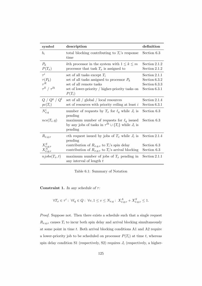
symbol description definition
bi total blocking contributing to Ti’s responsetime
Section 6.3
Pk kth processor in the system with 1 ≤ k ≤ m Section 2.1.2P (Tx) processor that task Tx is assigned to Section 2.1.2
τ i set of all tasks except Ti Section 2.1.1τ(Pk) set of all tasks assigned to processor Pk Section 6.3.2τR set of all remote tasks Section 6.3.3τ ll / τ lh set of lower-priority / higher-priority tasks on
P (Ti)Section 6.3.1
Q / Qg / Ql set of all / global / local resources Section 2.1.4pc(Ti) set of resources with priority ceiling at least i Section 6.3.1
N ix,q number of requests by Tx for `q while Ji is
pendingSection 6.3
ncs(Ti, q) maximum number of requests for `q issuedby any jobs of tasks in τ lh ∪ Ti while Ji ispending
Section 6.3
Rx,q,v vth request issued by jobs of Tx while Ji ispending
Section 2.1.4
XSx,q,v contribution of Rx,q,v to Ti’s spin delay Section 6.3
XAx,q,v contribution of Rx,q,v to Ti’s arrival blocking Section 6.3
njobs(Tx, t) maximum number of jobs of Tx pending inany interval of length t
Section 2.1.1
Table 6.1: Summary of Notation
Constraint 1. In any schedule of τ :
∀Tx ∈ τ i : ∀`q ∈ Q : ∀v, 1 ≤ v ≤ Nx,q : XAx,q,v +XS
x,q,v ≤ 1.
Proof. Suppose not. Then there exists a schedule such that a single request
Rx,q,v causes Ti to incur both spin delay and arrival blocking simultaneously
at some point in time t. Both arrival blocking conditions A1 and A2 require
a lower-priority job to be scheduled on processor P (Ti) at time t, whereas
spin delay condition S1 (respectively, S2) requires Ji (respectively, a higher-
125
priority job) to be scheduled on P (Ti) at time t. However, at any point in
time, at most one job can be scheduled on Ti’s processor.
We consider arrival blocking next. Since a job is released only once (and since
we assume that jobs do not self-suspend), each job can incur arrival blocking
only once (upon release). To express this, we use an indicator variable Aq,
with the following interpretation: given a fixed, concrete schedule, Aq = 1 if
and only if Ji incurred arrival blocking due to a critical section accessing `q,
and Aq = 0 otherwise. In a MILP interpretation, each Aq is a binary decision
variable. This allows us to formalize that at most one resource causes arrival
blocking.
Constraint 2. In any schedule of τ :∑
`q∈QAq ≤ 1.
Proof. Suppose not. Then there exists a schedule in which requests for two
different resources `1 and `2 both contribute to Ti’s arrival blocking. Arrival
blocking conditions A1 and A2 require a lower-priority job Jl to be scheduled
on processor P (Ti). Since we assume that Ji does not self-suspend, this is
only possible if Jl was already scheduled at the time of Ji’s release. Clearly,
only one such Jl exists. Since jobs become preemptable at the end of a
critical section, Jl would have to be accessing `1 and `2 simultaneously. Since
we assume that jobs hold at most one resource at a time, this is impossible.
Of course, in order for a resource `q to cause arrival blocking, it must
actually be accessed by local lower-priority tasks. Let τ ll denote the set
of local lower-priority tasks: τ ll , Tl | P (Tl) = P (Ti) ∧ l > i denote such
tasks.
126
Constraint 3. In any schedule of τ :
∀`q ∈ Q : Aq ≤∑Tx∈τ ll
Nx,q.
Proof. Suppose not. Then, since Aq is a binary variable, 1 = Aq >∑Tx∈τ ll Nx,q = 0 for some resource `q. By the definition of Aq, this implies
that Ti incurs arrival blocking due to requests for `q by local lower-priority
jobs although `q is not accessed by any local lower-priority tasks, which is
clearly impossible.
In a similar vein, we can rule out arrival blocking due to local resources with
priority ceilings lower than Ti’s priority (condition A2). To this end, we
let conflict set pc(Ti) of Ti denote the set of local resources with a priority
ceiling of at least Ti’s priority. Let Ql denote the set of local resources on
processor P (Ti). We define pc(Ti) as follows.
127
Def. 4: Conflict Set. Ti’s conflict set pc(Ti) is defined as`q∣∣ `q ∈ Ql ∧Π(`q) ≤ i
.
The next constraint rules our any arrival blocking due to requests to local
resources that are not in the conflict set.
Constraint 4. In any schedule of τ :
∀`q ∈ Ql \ pc(Ti) : Aq ≤ 0.
Proof. Follows from the definitions of the conflict set pc(Ti) and each Aq, as
Aq = 1 only if Ji is arrival-blocked due to a request for `q, which is possible
only if `q ∈ pc(Ti).
Another straightforward constraint on arrival blocking is that requests from
local higher-priority tasks cannot arrival-block Ti.
Constraint 5. In any schedule of τ :∑
Tx∈τ lh
∑q
N ix,q∑
v=1XAx,q,v ≤ 0.
Proof. Follows immediately from conditions A1 and A2, which require a
lower-priority job to be scheduled on P (Ti), whereas any job of tasks in τ lh
has higher priority than Ji.
The next constraint links the indicator variables Aq to the blocking variables
of local lower-priority tasks for `q.
Constraint 6. In any schedule of τ :
∀`q ∈ Q :∑Tx∈τ ll
N ix,q∑
v=1
XAx,q,v ≤ Aq.
Proof. Suppose not. If Aq = 0, this would imply, by definition of XAx,q,v, that
128
in some schedule Rx,q,v arrival-blocked Ji, even though by definition of Aq
no request for `q arrival-blocked Ji, which is clearly impossible. If Aq = 1,
at least two requests by local lower-priority tasks caused arrival blocking.
Analogously to Constraint 2, this is impossible because at most one request
can be in progress on P (Ti) when Ji is released.
Finally, we observe that spin delay is necessarily due to remote tasks,
since it is impossible to spin while waiting for local tasks. Analogously
to τ ll, we let τ lh denote the set of local higher-priority tasks: τ lh ,
Th | P (Th) = P (Ti) ∧ h < i.
Constraint 7. In any schedule of τ :∑
Tx∈τ ll∪τ lh
∑q
N ix,q∑
v=1XSx,q,v ≤ 0.
Proof. Suppose not. Then there exists a schedule in which at some point in
time t the execution of a request Rx,q,v issued by a local task Tx causes Ji to
incur spin delay. By conditions S1 and S2, a job on processor P (Ti) is also
spinning at time t. However, the job scheduled on P (Ti) at time t cannot
both be spinning and executing Rx,q,v at the same time.
This concludes our discussion of generic constraints and we now shift our focus
to spin lock type-specific constraints. We begin with F|N locks, because they
are the easiest to analyze, and because baseline analysis exists in the form of
Gai et al .’s classic MSRP analysis (summarized in Section 2.5.1).
6.3.2 Constraints for F|N Spin Locks
As discussed in Section 6.3, our analysis must explicitly account for transitive
delays to avoid the pessimism inherent in inflating job execution costs
(Theorem 3). In particular, the final blocking bound bi must represent all
delays that Ji may “accumulate” when higher-priority jobs that preempted Ji
129
spin. Thus, not only do we need to consider Ji’s requests for global resources,
but also any requests issued by higher-priority tasks. To this end, we let
ncs(Ti, q) denote an upper bound on the number of requests (or number of
critical sections) for `q issued either by Ji itself or by preempting higher-
priority jobs (while Ji is pending): ncs(Ti, q) , Ni,q +∑
Th∈τ lh Nix,q.
In conjunction with the strong progress guarantee in F|N locks, ncs(Ti, q)
implies an immediate upper bound on the number of requests for `q that
cause Ji to incur spin delay. Let τ(Pk) , Tx | P (Tx) = Pk be the set of
tasks assigned to Pk.
Constraint 8. In any schedule of τ with F|N locks:
∀`q ∈ Q : ∀Pk, Pk 6= P (Ti) :∑
Tx∈τ(Pk)
N ix,q∑
v=1
XSx,q,v ≤ ncs(Ti, q).
Proof. Suppose not. Then there exists a schedule in which more than
ncs(Ti, q) requests for some `q of tasks on processor Pk cause Ji to incur spin
delay. Then, by the pigeon-hole principle, at least one request for `q issued
by Ti or a local higher-priority task is delayed by more than one request for
`q from processor Pk. However, since jobs spin non-preemptably, and since
F|N locks serve requests in FIFO order, each request for `q can be preceded
by at most one request for `q from each other processor. Contradiction.
The above constraint, even though it may appear to be quite simple, is
considerably more effective at limiting blocking than prior analyses, as will
become evident in Section 6.7. Next, we apply the reasoning underlying
Constraint 8 to arrival blocking.
A remote job Jr can contribute to Ji’s arrival blocking if a local lower-priority
job Jl spins non-preemptably while waiting for Jr to release a lock. However,
130
at most one request from each processor can contribute to Ji’s arrival blocking
in this way.
Constraint 9. In any schedule of τ with F|N locks:
∀Pk, Pk 6= P (Ti) : ∀`q ∈ Q :∑
Tx∈τ(Pk)
N ix,q∑
v=1
XAx,q,v ≤ Aq.
Proof. Suppose not. If Aq = 0, then some request from a remote processor Pk
for resource `q causes Ji to incur arrival blocking. However, by the definition
of Aq, no requests for `q cause Ji to incur arrival blocking if Aq = 0. If
Aq = 1, then at least two requests for `q issued from processor Pk contribute
to Ti’s arrival blocking. Analogously to Constraint 2, at most one request of
a local lower-priority job Jl causes Ji to incur arrival blocking. Hence, at
least two requests from Pk must delay Jl. Analogously to Constraint 8, this
is impossible in F|N locks.
This concludes our analysis of F|N locks. The MILP for the analysis of F|N
locks consists of the generic Constraints 1–7 and the two Constraints 8 and 9
specific to F|N locks. If maximized, the objective value Equation (2) bounds
the maximum blocking incurred by any Ji. We proceed with the constraints
for the analysis of P|N locks.
6.3.3 Constraints for P|N Spin Locks
P|N locks ensure that a request is blocked at most once by another request
with lower priority at the expense that there is no immediate bound on the
number of blocking higher-priority requests. In the following, we denote the
locking priority of requests for resource `q issued by jobs of a task Tx as πx,q,
131

and the set of remote tasks with respect to Ti as τR:
τR , Tx | P (Tx) 6= P (Ti) .
We apply response-time analysis [19] on a per-request basis to obtain an upper
bound on the delay encountered when issuing a single request for a resource
`q with priority π. For a resource `q and task Ti, let WP|Nq (Ti, π) denote the
smallest positive value (if any) that satisfies the following recurrence:
W P|Nq (Ti, π) = S(`q, π) + LP(`q, π) + 1 where (3)
S(`q, π) =∑
Tx∈τR∧πx,q≤π
njobs(Tx,WP|Nq (Ti, π)) ·Nx,q · Lx,q and
LP(`q, π) = maxTx∈τR
Lx,q|πx,q > π.
The recurrence can be solved via fixed-point iteration. Since a bound
on the delay exceeding Ti’s deadline cannot be used as part of (effective)
constraints, the fixed-point iteration can be aborted if no fixed-point with
WP|Nq (Ti, π) ≤ di is found. If a solution for W
P|Nq (Ti, π) satisfying the above
recurrence can be found, then WP|Nq (Ti, π) bounds the delay of a single
request. We formalize this property with the following lemma.
Lemma 10. Let t0 be the time a job Ji of task Ti attempts to lock resource
`q with locking priority π, and let t1 be the time that Ji subsequently acquires
`q. With P|N locks, t1 − t0 ≤WP|Nq (Ti, π).
Proof. Analogous to the response-time analysis of non-preemptive fixed-
priority scheduling. The response-time of Ji’s request—that is, the maximum
wait time WP|Nq (Ti, π)—depends on the sum of the maximum length of one
lower-priority request LP(`q, π) and all higher-priority requests of all remote
tasks issued during an interval of length WP|Nq (Ti, π), that is, S(`q, π). Hence,
throughout an interval of length WP|Nq (Ti, π), by definition of W
P|Nq (Ti, π),
132
resource `q is unavailable for at most WP|Nq (Ti, π)− 1 time units. Thus, Ji’s
request is served after at most WP|Nq (Ti, π) time units after it was issued.
In the constraints we establish for the analysis of P|N locks, we exploit
two simple monotonicity properties of WP|Nq (Ti, π), which we next state
explicitly for the sake of clarity. First, WP|Nq (Ti, π) is monotonic with respect
to scheduling priority. That is, the wait time of a request for `q issued
by a local higher-priority task Th with the same locking priority π is no
longer than the wait time of Ti’s request. (In fact, the per-request wait-time
bound is independent of scheduling priority since jobs spin non-preemptably.)
Formally,
∀Th ∈ τ lh : W P|Nq (Ti, π) ≥W P|N
q (Th, π). (4)
The second monotonicity property that we exploit pertains to the locking
priority π: in a P|N lock, requests issued with higher locking priority natu-
rally do not incur more spin delay than requests issued with lower locking
priority:
π′ < π →W P|Nq (Ti, π) ≥W P|N
q (Ti, π′). (5)
The above monotonicity properties enables us to use wait-time bounds in
constraints computed with the minimum locking priority of any requests
issued by local higher and lower priority tasks, respectively. To simplify the
notation, we define
πminLPq , maxTx∈τ ll
πx,q|Nx,q > 0 and
πminHPq , maxTx∈(τ lh∪Ti)
πx,q|Nx,q > 0
133
to be the minimum locking priority of any lower-priority and higher-priority
task, respectively, on Ti’s processor that accesses the global resource `q. These
two definitions are needed because Ji might be delayed transitively due to
requests of local tasks with locking priorities lower than Ti’s own locking
priority. To obtain valid (and simple) constraints, we make the following
two simplifications: first, for a given resource `q, we assume that Ji and
all higher-priority jobs that preempt Ji issue requests with locking priority
πminHPq (the lowest locking priority that any such job uses), and second,
we assume that all local lower-priority jobs request `q with locking priority
πminLPq (again, the lowest locking priority used by any local lower-priority
job). Both of these are safe assumption due to the monotonicity property
stated in Equation (5). However, we note that these simplifications are a
potential source of pessimism that could be avoided with a significantly more
complicated analysis setup, which we leave to future work.
Given WP|Nq (Ti, π) (i.e., if it exists), we can constrain the the number of
requests for `q that can contribute to Ti’s spin delay. First, we consider
requests issued with higher or equal priority.
Constraint 10. In any schedule of τ with P|N locks:
∀Pk, Pk 6= P (Ti) : ∀`q ∈ Qg: ∀Tx ∈ τ(Pk), πx,q ≤ πminHPq :
N ix,q∑
v=1
XSx,q,v ≤ njobs(Tx,W
P|Nq (Ti, π
minHPq ))·Nx,q ·ncs(Ti, q).
Proof. Let R denote a request for a resource `q by Ti or a local higher-
priority task. By the definition of πminHPq , R has at least the locking priority
πminHPq and, by Lemma 10 and monotonicity properties of WP|Nq stated
in Equations (4) and (5), is hence delayed by at most WP|Nq (Ti, π
minHPq )
time units (note that WP|Nq (Ti, π
minHPq ) ≥ W
P|Nq (Th, πh,q) if Th ∈ τ lh and
πminHPq ≥ πh,q). During an interval of length WP|Nq (Ti, π
minHPq ), jobs of a
134
remote task Tx issue at most njobs(Tx,WP|Nq (Ti, π
minHPq )) · Nx,q requests
for `q. The stated bound follows as at most ncs(Ti, q) requests for `q with
a priority of at least πminHPq are issued by Ti or local higher-priority tasks.
Requests with lower priority cause Ji to incur (transitive) spin delay at most
once for each request by Ti or a task in τ lh.
Constraint 11. In any schedule of τ with P|N locks:
∀`q ∈ Qg :∑Tx∈τR
πx,q>πminHPq
N ix,q∑
v=1
XSx,q,v ≤ ncs(Ti, q).
Proof. Suppose not. Then at least one request for global resource `q issued
by Ti or a local higher-priority task is delayed more than once by a request
for `q from a different processor issued with a lower priority. However, by
definition P|N locks ensure that each request is blocked at most once by a
lower-priority request for the same resource. Contradiction.
Next, we consider arrival blocking. The number of lower-priority requests
that cause arrival blocking is bounded by Aq.
Constraint 12. In any schedule of τ with P|N locks:
∀`q ∈ Qg :∑Tx∈τR
πx,q>πminLPq
N ix,q∑
v=1
XAx,q,v ≤ Aq.
Proof. Suppose not. In case Aq = 0, by definition of Aq, Ti incurs transitive
arrival blocking due to a request for `q, although no access for `q from a local
lower-priority task causes Ti to incur arrival blocking, which is impossible.
In case Aq = 1, a request for `q with priority at least πminLPq is delayed
135
more than once by requests for `q issued on other processors with a locking
priority of less than πminLPq . However, with P|N locks, a request for a re-
source `q cannot be delayed by more than one lower-priority request for `q.
Contradiction.
Next, we constrain the arrival blocking due to requests with higher priority
issued from other processors.
Constraint 13. In any schedule of τ with P|N locks:
∀`q ∈ Qg : ∀Tx ∈ τR, πx,q ≤ πminLPq :
N ix,q∑
v=1
XAx,q,v ≤ njobs(Tx,W
P|Nq (Ti, π
minLPq )) ·Nx,q ·Aq.
Proof. Let R denote the request by a local lower-priority job that causes Ti
to incur arrival blocking. By definition of πminLPq , R has a priority of at least
πminLPq , and, by Lemma 10, is hence delayed by at most WP|Nq (Ti, π
minLPq )
time units (note that WP|Nq (Ti, π
minLPq ) ≥ W
P|Nq (Tl, πl,q) if Tl ∈ τ ll and
πminLPq ≥ πl,q). During an interval of length WP|Nq (Ti, π
minLPq ), jobs of a
remote task Tx issue at most njobs(Tx,WP|Nq (Ti, π
minLPq )) ·Nx,q requests for
`q. The bound follows as Ti is arrival-blocked via `q only if Aq = 1.
This concludes our analysis of P|N locks. Together with the generic Con-
straints 1–7, the P|N-specific Constraints 10–13 define a MILP that bounds
the maximum blocking incurred by any Ji. In the unlikely case that the re-
currence given in Equation (3) does not converge for some `q, Constraints 10
and 13 that depend on the wait-time bound WP|Nq (Ti, π) must be omitted
from the MILP for this resource `q.
Next, we present the constraints for the analysis of PF|N locks.
136
6.3.4 Constraints for PF|N Spin Locks
PF|N locks are a hybrid of the P|N locks and F|N locks considered previously:
they ensure that within each priority level requests are satisfied in FIFO
order, and each request can be delayed at most once by a lower-priority
request.
To begin with, similar to our analysis for P|N locks above, we establish a
wait-time bound that provides a bound on the maximum delay encountered
as part of single request for a resource `q issued with priority π. This wait-
time bound is then used in turn to bound the maximum interference due
to higher-priority requests. To this end, for a global resource `q, a task Ti,
and a priority π, let WPF|Nq (Ti, π) denote the smallest positive value that
satisfies the following recurrence:
W PF|Nq (Ti, π) , HP(`q, π) + SP(`q, π) + LP(`q, π) + 1. (6)
Here, HP(`q, π) denotes the maximum delay remote requests with a priority
higher than π can contribute to the wait time of Ji’s request, which can
be bounded based on the maximum number of jobs that exist during any
interval of length WPF|Nq (Ti, π):
HP(`q, π) =∑Tx∈τRπ>πx,q
(njobs
(Tx,W
PF|Nq (Ti, π)
)·Nx,q · Lx,q
).
SP(`q, π) accounts for the delay Ji’s request can incur due to remote requests
with priority π, which are served in FIFO order:
SP(`q, π) =
m∑Pk,Pk 6=P (Ti)
maxTx∈τ(Pk)
Lx,q|πx,q = π.
Finally, LP(`q, π) accounts for the delay Ji’s request can incur due to remote
137

lower-priority requests, which in a PF|N lock (similar to a P|N lock) is limited
to at most one critical section:
LP(`q, π) = maxTx∈τR
Lx,q|πx,q > π.
The fixed-point iteration can be aborted if no fixed-point with WPF|Nq (Ti, π) ≤
di is found. If the recurrence for WPF|Nq (Ti, π) converges, then it bounds the
delay of a single request for `q issued with priority π.
Lemma 11. Let t0 denote the time a job Ji of task Ti attempts to lock a
resource `q with locking priority π, and let t1 denote the time that Ji subse-
quently acquires the lock for `q. With PF|N locks, t1 − t0 ≤WPF|Nq (Ti, π).
Proof. Let R denote Ji’s request for `q. In a PF|N lock, at any point in time
t ∈ [t0, t1), Ji is spinning non-preemptably because either (i) `q is being used
by a job with locking priority (with respect to `q) lower than π, (ii) `q is
being used by a job with locking priority equal to π, or (iii) `q is being used
by a job with a locking priority greater than π. We bound the maximum
duration for which each of these conditions can hold during an interval of
length WPF|Nq (Ti, π).
Case (i): Since requests are satisfied in priority order when using PF|N
locks, R can be delayed by at most one lower-priority request for `q, which
is accounted for by LP(`q, π).
Case (ii): Since requests of equal priority are satisfied in FIFO order when
using PF|N locks, with respect to each other processor, R can be delayed
by at most one remote request for `q with priority π, for a total of at most
SP(`q, π) time units.
Case (iii): When using PF|N locks, any number of higher-priority requests
can delay R. However, analogous to the response-time analysis of non-
preemptive fixed-priority scheduling, the maximum number of higher-priority
138
requests for `q that exist during [t0, t1) bounds the length of the interval since
Ji ceases spinning and acquires `q as soon as `q is no longer contended. In any
interval of length WPF|Nq (Ti, π), at most njobs
(Tx,W
PF|Nq (Ti, π)
)jobs of each
remote task Tx with a locking priority πx,q higher than π exist. Each such job
issues at most Nx,q requests for `q, and holds `q for at most Lx,q time units as
part of each request. Each remote task Tx with a higher locking priority (with
respect to `q) hence holds `q for at most njobs(Tx,W
PF|Nq (Ti, π)
)·Nx,q ·Lx,q
during any interval of length WPF|Nq (Ti, π). The term HP(`q, π) thus bounds
the cumulative length that Ji is spinning while a job with a higher locking
priority uses `q during any interval of length WPF|Nq (Ti, π).
Since WPF|Nq (Ti, π) is by definition the smallest value that satisfies Equa-
tion (6) (if one exists), after at most WPF|Nq (Ti, π) time units after Ji started
spinning, `q is no longer unavailable due to a lower-priority (with respect to
`q) request (case (i)), `q is no longer unavailable due to earlier-issued equal-
priority requests (case (ii)), and `q is no longer contended by jobs of tasks
with higher locking priority (case (iii)). Hence, throughout an interval of
length WPF|Nq (Ti, π), resource `q is unavailable for at most W
PF|Nq (Ti, π)− 1
time units. Thus, Ji’s request is served after at most WPF|Nq (Ti, π) time
units after it was issued.
If WPF|Nq (Ti, π) does not exist, that is, if the recurrence Equation (6) does
not converge, then starvation cannot be ruled out and Constraints 14 and 15
do not apply.
Similar to the monotonicity properties of WP|Nq (Ti, π) (Equations (4) and (5)),
WPF|Nq (Ti, π) is monotonic with respect to scheduling priority and locking
priority:
∀Th ∈ τ lh : W PF|Nq (Ti, π) ≥W PF|N
q (Th, π) and (7)
139
π′ < π →W PF|Nq (Ti, π) ≥W PF|N
q (Ti, π′). (8)
Based on the wait-time bound WPF|Nq (Ti, π), we next present constraints on
the maximum spin delay incurred by any Ji when using PF|N locks. Recall
from Section 6.3.3 that πminLPq and πminHP
q denote the minimum locking
priority of any lower-priority and higher-priority task, respectively, on Ti’s
processor that accesses the global resource `q. For convenience, we repeat
the definitions here:
πminLPq , max
Tx∈τ llπx,q|`q ∈ Q ∧Nx,q > 0,
πminHPq , max
Tx∈(τ lh∪Ti)πx,q|`q ∈ Q ∧Nx,q > 0.
Similar to Constraint 10 for P|N locks, we can impose a simple constraint on
the maximum spin delay due to higher-priority requests.
Constraint 14. In any schedule of τ with PF|N locks:
∀Pk, Pk 6= P (Ti) : ∀`q ∈ Qg : ∀Tx ∈ τ(Pk), πx,q < πminHPq :
N ix,q∑
v=1
XSx,q,v ≤ njobs
(Tx,W
PF|Nq (Ti, π
minHPq )
)·Nx,q · ncs(Ti, q).
Proof. Analogous to Constraint 10. Each request R for `q issued by Ji
remains incomplete for at most WPF|Nq (Ti, π) time units. Due to the mono-
tonicity property stated in Equation (7), this also holds true for any request
issued for `q by a job of a higher-priority task that preempted Ji. At most
ncs(Ti, q) requests are issued for `q by Ti and local higher-priority tasks
while Ji is pending. Hence at most ncs(Ti, q) ·njobs(Tx,W
PF|Nq (Ti, π)
)·Nx,q
requests of each remote task Tx with higher locking priority delay Ji.
140
Next, we establish a constraint on arrival blocking due to the non-preemptable
spinning of lower-priority jobs that are delayed by remote requests with higher
locking priority.
Constraint 15. In any schedule of τ with PF|N locks:
∀`q ∈ Qg : ∀Tx ∈ τR, πx,q < πminLPq :
N ix,q∑
v=1
XAx,q,v ≤ njobs
(Tx,W
PF|Nq (Ti, π
minLPq )
)·Nx,q ·Aq.
Proof. Analogous to Constraint 13. A request R issued by a local lower-
priority task (with priority at least πminLPq ) can be delayed by all remote
requests for `q with higher locking priorities. Exploiting Equations (7) and (8),
R remains incomplete for at most WPF|Nq (Ti, π
minLPq ) time units, which limits
the maximum number of jobs of each remote task Tx with a (potentially)
higher locking priority to njobs(Tx,W
PF|Nq (Ti, π
minLPq )
). The stated bound
on the maximum number of transitively blocking remote requests with higher
locking priorities follows.
Requests issued with the same locking priority are satisfied in FIFO order.
Hence, the spin delay due to remote equal-priority requests can be constrained
similarly to how it is constrained in the analysis of F|N locks.
Constraint 16. In any schedule of τ with PF|N locks:
∀Pk, Pk 6= P (Ti) : ∀`q ∈ Qg :∑
Tx∈τ(Pk)πx,q=πminHP
q
N ix,q∑
v=1
XSx,q,v ≤ ncs(Ti, q).
Proof. Analogous to Constraint 8. Due to the FIFO-ordering of equal-priority
requests, it follows that, with respect to each remote processor, at most one
141
earlier-issued, equal-priority request can delay each of the ncs(Ti, q) requests
for `q issued by Ji and local higher-priority jobs.
As mentioned before, assuming that all requests for `q issued by Ji and local
higher-priority jobs are issued with locking priority πminHPq is safe due to
the monotonicity property stated in Equation (8); the blocking incurred by
any Ji does not exceed the bound implied by Constraint 16 if in the actual
schedule some requests of Ji or local higher-priority jobs are issued with a
locking priority higher than πminHPq .
Next, we constrain the maximum transitive delay due to the non-preemptable
spinning of lower-priority jobs that are delayed by earlier-issued remote
requests with equal locking priority.
Constraint 17. In any schedule of τ when using PF|N locks:
∀`q ∈ Qg : ∀Pk, Pk 6= P (Ti) :∑
Tx∈τ(Pk)πx,q=πminLP
q
N ix,q∑
v=1
XAx,q,v ≤ Aq.
Proof. Analogous to Constraint 9. Since requests with the same priority are
served in FIFO-order, at most one request per processor for a resource `q is-
sued with the same locking priority can contribute to Ti’s arrival blocking.
Finally, we constrain the maximum spin delay due to remote requests with
lower locking priority.
Constraint 18. In any schedule of τ with PF|N locks:
∀`q ∈ Qg :∑Tx∈τR
πx,q>πminHPq
N ix,q∑
v=1
XSx,q,v ≤ ncs(Ti, q).
142
Proof. Analogous to Constraint 11. Each request for `q issued by Ti or a
local higher-priority job can be delayed at most once by a remote request for
`q issued with a lower priority.
Similar reasoning applies to the maximum transitive delay due to the non-
preemptable spinning of a lower-priority job that is delayed by a remote
request with a lower locking priority.
Constraint 19. In any schedule of τ with PF|N locks:
∀`q ∈ Qg :∑Tx∈τR
πx,q>πminLPq
N ix,q∑
v=1
XAx,q,v ≤ Aq.
Proof. Analogous to Constraint 12. If Ji is transitively blocked due to a
request for `q (i.e., if Aq = 1), then at most one remote request for `q issued
with a priority less than πminLPq can contribute to Ti’s arrival blocking.
This concludes our analysis of PF|N locks. Together with the generic Con-
straints 1–7, the PF|N-specific Constraints 14–19 define a MILP that bounds
the maximum blocking incurred by any Ji. In the unlikely case that the re-
currence given in Equation (6) does not converge for some `q, the constraints
that depend on the wait-time bound WPF|Nq (Ti, π), namely Constraints 14
and 15, must be omitted from the MILP for this resource `q.
Next, we present constraints for the analysis of preemptable spin locks. We
start with generic constraints applicable to all preemptable types considered
in this work.
143

6.3.5 Generic Constraints for Preemptable Spin Locks
The generic constraints described in Section 6.3.1 all remain applicable for the
analysis of preemptable spin locks. Allowing preemptions while busy-waiting
for global resources enables us to impose an additional generic constraint:
while busy-waiting, jobs are subject to normal fixed-priority scheduling, and
hence, spinning never causes a priority inversion. Requests from remote
tasks thus cannot cause (transitive) arrival blocking. We express this with
the following constraint.
Constraint 20. In any schedule of τ with preemptable spin locks:
∑Tx∈τR
∑`q∈Q
N ix,q∑
v=1
XAx,q,v ≤ 0.
Proof. Follows from the preceding discussion.
Preemptable spinning solves the transitive arrival blocking problem, but it
does so at the expense of increasing spin delays. Recall from Section 2.4.2
that a job that is preempted while spinning re-issues its request once it
resumes execution and continues spinning. To accurately account for these
“retries” due to preemptions, we introduce a new indicator variable: for each
resource `q, with respect to an arbitrary, but fixed schedule, let Cq denote
the number of times that a request for resource `q by Ji or a job of a task
in τ lh is canceled due to a preemption. From a MILP point of view, each
Cq is an integer variable. Note that each preemption can cause at most
one request to be canceled (since at most one job may be spinning at any
time). A trivial bound on the sum of all Cq is then given by the number
of higher-priority job releases that can possibly occur while Ji is pending.
The following constraint limits Cq to the number of local higher-priority job
144
releases, so that Cq can be later used in other constraints.
Constraint 21. In any schedule of τ with preemptable spin locks:
∑`q
Cq ≤∑
Th∈τ lh
⌈riph
⌉.
Proof. Follows from the preceding discussion.
Another trivial observation is that Cq = 0 if neither Ji nor any higher-priority
jobs access `q.
Constraint 22. In any schedule of τ with preemptable spin locks:
∀`q : if ncs(Ti, q) = 0 then Cq = 0.
Proof. By definition of Cq. If neither Ti nor any local higher-priority tasks
issue requests for `q, then no such request can be canceled.
We use Cq in the following for spin lock type-specific constraints, and we
begin with constraints for the analysis of F|P locks.
6.3.6 Constraints for F|P Spin Locks
As Cq bounds the number of times that a particular resource is re-requested,
we can almost directly apply the argument of Constraint 8 for F|N spin locks;
the only change is that each time that `q is re-requested, requests issued
from other processors may “skip ahead” once.
145

Constraint 23. In any schedule of τ with F|P locks: ∀`q ∈ Q :
∀Pk, Pk 6= P (Ti) :∑
Tx∈τ(Pk)
N ix,q∑
v=1
XSx,q,v ≤ ncs(Ti, q) + Cq.
Proof. Suppose not. Then more than ncs(Ti, q)+Cq requests by tasks on a re-
mote processor Pk for a resource `q contribute to Ti’s spin delay. As requests
are issued sequentially and served in FIFO order, Ti and local higher-priority
jobs issue at most ncs(Ti, q) +Cq requests for `q (counting requests re-issued
after a preemption as individual requests). By the pigeon-hole principle,
this implies that one firstly issued request or one re-issued request (possibly
both) for `q issued by Ti or local higher-priority jobs was blocked by more
than one request issued by jobs on Pk. With FIFO-ordered spin locks, this
is impossible.
Note that, in contrast to F|N locks, we do not impose any constraints
pertaining to arrival blocking specific to F|P. With preemptable spinning,
remote requests cannot cause any arrival blocking and this is already ruled
out by Constraint 20. Hence, a constraint analogous to Constraint 9 for F|N
locks is not required.
This concludes our analysis of F|P locks. Preemptable spinning increases the
analysis complexity (additional integer variables are required) and increases
spin delays (Constraint 23 permits more blocking than Constraint 8 since
canceled request due to preemptions have to be retried), but with our MILP-
based analysis approach, both aspects can be easily integrated. To the
best of our knowledge, this is the first analysis of preemptable spin locks
from a worst-case blocking point of view. Next, present the constraints for
priority-ordered spin locks.
146
6.3.7 Constraints for P|P Spin Locks
Priority-ordered preemptable spin locks ensure that each request is delayed
at most once by a different request with a lower priority. For requests with
the same priority no particular ordering is specified.
Similar to the non-preemptable spin locks based on priority-ordering (i.e.,
P|N and PF|N), we first establish a wait-time bound to bound the worst-case
delay that a job of Ti can incur after issuing a request for a resource `q (with
priority πi,q) until the request is satisfied.
For a global resource `q and a task Ti, let WP|Pq (Ti) denote the smallest
positive value that satisfies the following recurrence:
W P|Pq (Ti) = S(Ti, `q) + LP i(Ti, `q) + LP lh(Ti, `q)
+ I(Ti, `q) + LPP (Ti, `q) + 1. (9)
The individual components of WP|Pq (Ti) are defined as follows and justified
in the proof of Lemma 12 below.
S(Ti, `q) bounds the maximum delay remote requests of equal or higher
priority can contribute to the wait time of Ti’s request. However, since Ji can
be preempted while spinning, “equal or higher priority” has to be interpreted
with respect to the lowest locking priority used by either Ti (when accessing
`q) or a local higher-priority job (when accessing any resource). S(Ti, `q)
thus accounts for all delays due to both Ti’s request and requests of local
higher-priority tasks being blocked by remote requests of higher or equal
priority:
S(Ti, `q) =∑
`r∈Qlh∪`q
∑Tx∈τRπx,r≤π′r
(njobs
(Tx,W
P|Pq (Ti)
)·Nx,r · Lx,r
),
147
where
π′r =
maxπh,r | Th ∈ τ lh ∧Nh,r > 0 if `r 6= `q
maxπh,r | Th ∈ τ lh ∪ Ti ∧Nh,r > 0 if `r = `q.
LP i(Ti, `q) accounts for the time Ji’s request can be delayed by a remote
lower-priority request that already held `q when Ji issued its request:
LP i(Ti, `q) = maxTx∈τR
Lx,q|πx,q > πi,q.
LP lh(Ti, `q) accounts for requests from local higher-priority jobs that are
delayed by remote lower-priority requests:
LP lh(Ti, `q) =∑
`r∈Qlh
∑Th∈τ lh
⌈W
P|Pq (Ti)
ph
⌉·Nh,r · max
Tx∈τRLx,q|πx,r > πh,r.
In a P|P lock, Ji can be preempted while busy-waiting, and hence interference
due to the execution of local higher-priority jobs needs to be accounted for
with I(Ti, `q):
I(Ti, `q) =∑
Th∈τ lh
⌈W
P|Pq (Ti)
ph
⌉· eh.
Finally, LPP (Ti, `q) accounts for the (possibly transitive) delay that results
from Ji or a higher-priority job being preempted while spinning:
LPP (Ti, `q) = prts(Ti,W
P|Pq (Ti)
)· cpp(Ti, `q).
Here, prts(Ti, t) denotes the maximum number of preemptions that occur
on Ti’s processor throughout any interval of length t while a job of Ti is
148
pending:
prts(Ti, t) ,∑
Th∈τ lh
⌈t
ph
⌉.
And cpp(Ti, `q) denotes the worst-case cost per preemption (of either Ji or a
local higher-priority job) with respect to the increase in Ji’s waiting time
due to a remote lower-priority request acquiring a contested resource:
cpp(Ti, `q) = maxcpp lh(Ti), cppi(Ti, `q),
where cpp lh(Ti) denotes the worst-case cost per preemption of a higher-
priority job, formally,
cpp lh(Ti) = maxLx,r | Tx ∈ τR ∧ `r ∈ Qlh ∧
Th ∈ τ lh ∧ Nh,r > 0 ∧
πh,r < πx,r,
and where cppi(Ti, `q) denotes the worst-case cost per preemption of Ji,
formally,
cppi(Ti, `q) = maxLx,q | Tx ∈ τR ∧ πi,q < πx,q.
The fixed-point iteration can be aborted if no fixed-point with WP|Pq (Ti, π) ≤
di is found. If the recurrence for WP|Pq (Ti, π) converges, then it bounds the
delay of a single request for `q issued with priority π.
Lemma 12. Let t0 denote the time a job Ji of task Ti attempts to lock
a resource `q (with its assigned locking priority πi,q), and let t1 denote
the time that Ji subsequently acquires the lock for `q. With P|P locks,
t1 − t0 ≤WP|Pq (Ti).
149
Proof. Analogous to Lemma 11. Let R denote Ji’s request for `q. In any point
in time t ∈ [t0, t1), Ji is either spinning or has been preempted by a local
higher-priority job. We distinguish among seven different cases, depending
on whether Ji is scheduled or preempted, whether a spinning job was already
preempted, and whether a lower- or higher-priority request causes blocking
at time t.
If Ji is spinning at time t, then R is blocked because `q is being used by
a remote job Jx at time t. We consider three distinct cases: (i) Jx has a
locking priority (with respect to `q) of at least πi,q, (ii) Jx has a locking
priority (with respect to `q) lower than πi,q and Ji has not been preempted
during [t0, t], or (iii) Jx has a locking priority (with respect to `q) lower than
πi,q and Ji has previously been preempted during [t0, t).
Otherwise, if Ji has been preempted and a local higher-priority job Jh is
scheduled at time t, then Jh is either (iv) executing normally, or it is spinning
(which transitively delays Ji). If Jh is spinning, it requested some resource
`r (not necessarily `q) that is currently in use by a remote job Jx. We again
distinguish among three cases: (v) Jx’s locking priority is at least as high
as Jh’s locking priority (both with respect to `r), (vi) Jx’s locking priority
is lower than Jh’s locking priority (both with respect to `r) and Jh has not
been preempted while busy-waiting for `r, and (vii) Jx’s locking priority is
lower than Jh’s locking priority (both with respect to `r) and Jh has been
preempted while busy-waiting for `r.
We bound the maximum duration for which each of these conditions can
hold during an interval of length WP|Pq (Ti). We begin with requests of equal
or higher priority delaying either Ji or a local higher-priority job.
Cases (i) and (v): In cases (i) and (v), in order for a remote task Tx to
(transitively) delay Ji, it must either be using `q and have a locking priority
πx,q ≤ πi,q, or it must be using some `r ∈ Qlh (where possibly `q = `r)
150
and have a locking priority higher than or equal to the locking priority
of some task Th ∈ τ lh that accesses `r (i.e., Nh,r > 0 and πx,q ≤ πh,r).
The cumulative length of all critical sections of all remote tasks satisfying
either condition, which is given by S(Ti, `q), thus bounds the total duration
during which either case (i) or case (v) occurs during an interval of length
WP|Pq (Ti).
Case (ii): If Ji is delayed by a job Jx using `q, and Jx has a lower locking
priority than Ji and Ji has not been preempted during [t0, t], then Jx must
have continuously used `q during [t0, t] since P|P locks ensure that jobs with
lower locking priority cannot acquire `q while Ji is spinning. The maximum
critical section length of any remote task Tx with πx,q > πi,q, as given
by LP i(Ti, `q), thus bounds the maximum duration during which case (ii)
occurs.
Cases (iii) and (vii): In P|P locks, if Ji is preempted while busy-waiting,
then remote jobs with a locking priority lower than πi,q may acquire `q while
Ji is preempted, which may lead to case (iii). Similarly, if a local higher-
priority job Jh is preempted while busy-waiting for a resource `r ∈ Qlh,
remote jobs with a locking priority lower than πh,r may acquire `r while
Jh is preempted, which may lead to case (vii). In both cases, additional
(transitive) delay is caused by the preemption as Ji’s wait time is increased
by the length of one lower-priority critical section. That is, each time that
Ji is preempted, Ji may spin for up to an additional cppi(Ti, `q) time units
when resuming execution, and each time that a local higher-priority job Jh
is preempted while spinning, Ji may be transitively delayed for up to an
additional cpp lh(Ti) time units when Jh resumes execution, for a worst-case
cost per preemption of cpp(Ti, `q). During an interval of length WP|Pq (Ti), at
most prts(Ti,W
P|Pq (Ti)
)higher-priority jobs are released on Ji’s processor,
which bounds the total number of preemptions. Hence the total cumulative
duration during which either case (iii) or case (vii) occurs over the course of
151

an interval of length WP|Pq (Ti) is bounded by LPP (Ti, `q).
Case (iv): Analogously to the regular response-time analysis of (preemptive)
fixed-priority scheduling [19], during an interval of length WP|Pq (Ti) starting
at time t0 (at which no higher-priority jobs can be pending because Ji is
scheduled and tasks are assumed to not self-suspend), each local higher-
priority task Th ∈ τ lh releases at most
⌈W
P|Pq (Ti)ph
⌉jobs, each of which
executes for at most eh time units (not counting any spinning). The total
delay due to the regular execution of higher-priority jobs during an interval
of length WP|Pq (Ti) starting at time t0 is hence bounded by I(Ti, `q).
Case (vi): Analogously to case (ii), if a higher-priority job Jh trying to lock
a resource `r ∈ Qlh is not preempted, it spins waiting for a task Tx ∈ τR
with πx,r > πh,r to release `r for at most the duration of one critical section.
During an interval of length WP|Pq (Ti), each higher-priority task Th releases
at most
⌈W
P|Pq (Ti)ph
⌉jobs, each of which accesses each `r ∈ Qlh at most Nh,r
times. As part of each such access, case (vi) occurs for the duration of at
most one critical section. The total duration of case (vi) occurring during an
interval of length WP|Pq (Ti) is hence bounded by LP lh(Ti, `q).
This covers all possible ways in which Ji may be (transitively) delayed when
trying to lock a resource `q. Therefore, during an interval of length WP|Pq (Ti),
the total delay incurred by Ji—that is, the total duration during which one
of the seven analyzed cases occurs—is limited to S(Ti, `q) + LP i(Ti, `q) +
LPP (Ti, `q) + I(Ti, `q) + LP lh(Ti, `q) = WP|Pq (Ti)− 1. In other words, during
an interval of length WP|Pq (Ti) starting at time t0, Ji is unable to lock `q for
at most WP|Pq (Ti)− 1 time units. Ji thus ceases to spin and acquires `q at
time t1 at most WP|Pq (Ti) time units after initially trying to lock `q.
In the following, we assume that the wait-time bound WP|Pq (Ti), i.e., the
smallest integer to satisfy Equation (9), can be computed via fixed-point
152

iteration. If, however, the fixed-point iteration does not converge, then the
per-request maximum wait-time of Ji (with respect to `q) cannot be bounded
with the presented approach and Constraint 24 below cannot be applied.
(Constraint 25 remains valid in either case.)
As before in the analysis of PF|N locks, we exploit that WP|Pq (Ti) is monotonic
with respect to scheduling priority. That is, the wait-time bound for a
local higher-priority task Th is no longer than the wait-time bound for Ti.
Formally,
∀Th ∈ τ lh : W P|Pq (Ti, π) ≥W P|P
q (Th, π). (10)
Note that Equation (10) depends specifically on the definitions of S(Ti, `q),
since S(Ti, `q) is defined in terms of the minimum locking priority of Ti and
all local higher-priority tasks, which ensures the required monotonicity.
Given the wait-time bound WP|Pq (Ti), we can constrain the the number of
requests for `q that can contribute to Ti’s spin delay, similar to Constraint 10.
First, we consider requests issued with higher or equal priority. As in the
analysis of PF|N locks, we make the simplifying assumption that all higher-
priority jobs issue requests for each `q with locking priority πminHPq .
Constraint 24. In any schedule of τ when using P|P locks:
∀Pk, Pk 6= P (Ti) : ∀`q ∈ Qg : ∀Tx ∈ τ(Pk), πx,q ≤ πminHPq :
N ix,q∑
v=1
XSx,q,v ≤ njobs
(Tx,W
P|Pq (Ti)
)·Nx,q · ncs(Ti, q).
Proof. Analogous to Constraint 10. Due to the monotonicity property stated
in Equation (10), it is safe to use WP|Pq (Ti) to bound the maximum duration
of any request issued by Ji or any local higher-priority tasks. Each request
R for `q issued by Ti or a local higher-priority task has a locking priority of
153

at least πminHPq . During any interval of length WP|Pq (Ti), jobs of a remote
task Tx with locking priority at least πminHPq (with respect to `q) issue at
most njobs(Tx,W
P|Pq (Ti)
)·Nx,q requests for `q. The stated bound follows
since Ji and higher-priority jobs issue at most ncs(Ti, q) requests for `q.
Next, we consider blocking requests of lower locking priority. Requests with
lower locking priority can (possibly transitively) cause Ti to incur spin delay
at most once for each request issued by Ti or a local higher-priority task.
Further, Ji can be (possibly transitively) blocked by a remote lower-priority
request each time Ji or a local higher-priority job is preempted. (Recall that
Ji and local higher-priority jobs are preempted at most Cq times in total while
busy-waiting for `q, which is enforced with Constraints 21 and 22.)
Constraint 25. In any schedule of τ when using P|P locks:
∀`q ∈ Qg :∑Tx∈τR
πx,q>πminHPq
N ix,q∑
v=1
XSx,q,v ≤ ncs(Ti, q) + Cq.
Proof. Analogous to Constraints 23 and 11. Each request R for `q issued by
Ti or a local higher-priority task has a locking priority of at least πminHPq .
Ji can be directly or transitively delayed be remote lower-priority requests
for a resource `q each time Ji or a local higher-priority task is preempted
or issues a request for `q. Hence the total number of times that Ji or local
higher-priority jobs busy-wait for `q, in addition to the number of times
that Ji or local higher-priority jobs need to restart busy-waiting after being
preempted, limits the number of requests issued with locking priority lower
than πminHPq that (transitively) delay Ji.
This concludes our analysis of P|P locks. Together with the generic Con-
154

straints 1–7 (for any lock type), and the generic Constraints 20–22 (for
preemptable spin locks), the P|P-specific Constraints 24 and 25 define a
MILP that bounds the maximum blocking incurred by any Ji. If the recur-
rence given in Equation (9) does not converge for some `q, Constraint 24
must be omitted from the MILP for that resource `q.
6.3.8 Constraints for PF|P Spin Locks
Like their non-preemptable counterpart PF|N locks, PF|P locks are a hybrid
of FIFO-ordered and priority-ordered spin locks. For requests with different
priorities, PF|P locks behave similar to P|P locks: a request can be blocked
by at most once one other request for the same resource issued with lower
locking priority, while a request can be blocked by all concurrent higher-
priority requests for the same resource. Requests with the same locking
priority, however, are served in FIFO-order. This similarity of PF|P locks
to P|P locks is also reflected in the approach that we employ to analyze
PF|P locks: similar to P|P locks, we first establish a wait-time bound on
the worst-case delay that a job of Ti can incur when attempting to lock a
resource `q. This bound is later used in Constraint 26 to limit the number
of requests that can contribute to Ti’s overall blocking.
For a global resource `q and a task Ti, let WPF|Pq (Ti) denote the smallest
positive value that satisfies the following recurrence:
W PF|Pq (Ti) = HP(Ti, `q) + LSP i(Ti, `q) + LSP lh(Ti, `q)
+ LSPP (Ti, `q) + I(Ti, `q) + 1. (11)
The individual components of WPF|Pq (Ti) are defined as follows and justified
in the proof of Lemma 13.
HP(Ti, `q) denotes the maximum delay that remote higher-priority requests
155

for `q or any other resources requested by local higher-priority tasks can
contribute to the wait time of Ti’s request:
HP(Ti, `q) =∑
`r∈Qlh∪`q
∑Tx∈τRπx,r<π′r
(njobs
(Tx,W
PF|Pq (Ti)
)·Nx,r · Lx,r
),
where
π′r =
maxπh,r | Th ∈ τ lh ∧Nh,r > 0 if `r 6= `q
maxπh,r | Th ∈ τ lh ∪ Ti ∧Nh,r > 0 if `r = `q.
(12)
To define the remaining terms, we first define a generic helper bound
spinLS (Pa, `r, π) that bounds the maximum delay due to requests of equal
and lower priority only that any job Ja that starts (or restarts) busy-waiting
on a processor Pa for a resource `r with locking priority π incurs before
either acquiring `r or being preempted (and thus being forced to restart
busy-waiting). There are two cases that must be considered: Ja could be
delayed by up to m− 1 requests issued by remote jobs with equal locking
priority, or by one request issued by a remote job with lower locking priority
and up to m− 2 requests issued by remote jobs with equal locking priority.
We therefore define spinLS (Pa, `r, π) as:
spinLS (Pa, `r, π) = max
spinS (Pa, `r, π), spinL(Pa, `r, π),
where spinS (Pa, `r, π) bounds the maximum delay when (up to) m − 1
jobs with equal locking priority precede Ja in the queue for `r, and where
spinL(Pa, `r, π) bounds the case of Ja being preceded by one lower-priority
and up to m− 2 equal-priority requests.
A safe bound on spinS (Pa, `r, π) is given by the sum of the maximum critical
156
lengths on each remote processor:
spinS (Pa, `r, π) =∑Pk 6=Pa
max Lx,r | Tx ∈ τ(Pk) ∧ πx,r = π .
If a job with a lower locking priority holds `r when Ja starts busy-waiting,
only (up to) m− 2 jobs with equal locking priority precede Ja in the queue
for `r (recall that jobs are removed from the queue when they are preempted,
and that only one job per processor is spinning at any time). Suppose that
the job with lower locking priority executes on processor Pl. Then a safe
bound is given by:
spinL′(Pa, `r, π, Pl) = max Lx,q|Tx ∈ τ(Pl) ∧ πx,q > π
+∑
Pk 6=P (Ti)Pk 6=Pl
max Lx,q|Tx ∈ τ(Pk) ∧ πx,q = π .
Since the job with lower locking priority could potentially reside on any
processor (other than Pa), spinL(Pa, `r, π) is defined as follows:
spinL(Pa, `r, π) = maxPl 6=Pa
spinL′(Pa, `r, π, Pl)
.
With the definition of spinLS (Pa, `r, π) in place, it is easy to express the
remaining terms.
LSP i(Ti, `q) accounts for the time Ji’s request can be delayed by remote
requests with a lower or equal locking priority (before Ji is preempted, if at
all):
LSP i(Ti, `q) = spinLS (P (Ti), `q, πi,q).
LSP lh(Ti, `q) accounts for spinning local higher-priority jobs that are delayed
157
by remote requests issued with the same or lower locking priority:
LSP lh(Ti, `q) =∑lr∈Qlh
∑Th∈τ lh
⌈W
PF|Pq (Ti)
ph
⌉·Nh,r · spinLS (P (Ti) , `r, πh,r) .
Since busy-waiting jobs can be preempted in PF|P locks, I(Ti, `q) accounts for
the interference that Ji can incur due to the execution of local higher-priority
jobs:
I(Ti, `q) =∑
Th∈τ lh
⌈W
PF|Pq (Ti)
ph
⌉· eh.
Preemptions can also cause additional spinning because other jobs may “skip
ahead” in the wait queue when a busy-waiting job is preempted. To account
for this, LSPP (Ti, `q) bounds the additional delay Ji can incur (possibly
transitively) due to the preemption of Ji and local higher-priority jobs:
LSPP (Ti, `q) = cpp(Ti, `q) · prts(Ti,W
PF|Pq (Ti)
),
where prts(Ti, t) is defined as before in the analysis of P|P locks. The
definition of cpp(Ti, `q), which denotes the worst-case cost per preemption
(of either Ji or a local higher-priority job) with respect to the increase in
Ji’s wait time due to a remote request acquiring a contested resource, is also
defined as in the analysis of P|P locks:
cpp(Ti, `q) = max
cpp lh(Ti), cppi(Ti, `q).
The definitions of cpp lh(Ti) and cppi(Ti), however, must be adjusted to
reflect the FIFO-ordering of equal-priority requests in PF|P locks. cppi (Ti, `q)
bounds the maximum additional delay incurred by Ji when it is forced to
158
restart its request for `q after being preempted, where
cppi(Ti, `q) = spinLS (P (Ti), `q, πi,q).
Analogously, cpp lh(Ti) bounds the maximum additional delay transitively
incurred by Ji after a preemption of a higher-priority job Jh that is busy-
waiting for a resource `r ∈ Qlh. Since a higher-priority job might be waiting
for any resource in Qlh when it is preempted, and since the identity of Jh is
not known a priori, a safe bound is given by:
cpp lh(Ti) = max
spinLS (P (Ti), `r, πh,r) | Th ∈ τ lh ∧Nh,r > 0.
The fixed-point iteration can be aborted if no fixed-point with WPF|Pq (Ti, π) ≤
di is found. If the recurrence for WPF|Pq (Ti, π) converges, then it bounds the
delay of a single request for `q issued with priority π.
Lemma 13. Let t0 denote the time a job Ji of task Ti attempts to lock
a resource `q (with its assigned locking priority πi,q), and let t1 denote
the time that Ji subsequently acquires the lock for `q. With PF|P locks,
t1 − t0 ≤WPF|Pq (Ti).
Proof. Analogous to the proof of Lemma 12. Let R denote Ji’s request for
`q. In any point in time t ∈ [t0, t1), J1 is spinning or preempted by a local
higher-priority job. We distinguish among eleven different scenarios, which
together cover all possible ways in which Ji can be prevented from acquiring
`q at time t.
If Ji is spinning at time t, then R is blocked because `q is being used by a
remote job Jx at time t. We consider five distinct cases: (i) Jx has a locking
priority (with respect to `q) exceeding πi,q, (ii) Jx has a locking priority
(with respect to `q) equal to πi,q and Ji has not been preempted during [t0, t],
(iii) Jx has a locking priority (with respect to `q) equal to πi,q and Ji has
159

previously been preempted during [t0, t], (iv) Jx has a locking priority (with
respect to `q) lower than πi,q and Ji has not been preempted during [t0, t),
or (v) Jx has a locking priority (with respect to `q) lower than πi,q and Ji
has previously been preempted during [t0, t).
Otherwise, if Ji has been preempted and a local higher-priority job Jh is
scheduled at time t, then Jh is either (vi) executing normally, or it is spinning.
If Jh is spinning, it requested some resource `r ∈ Qlh that is currently in
use by a remote job Jx. We again distinguish among five cases: (vii) Jx’s
locking priority is higher than Jh’s locking priority (both with respect to `r),
(viii) Jx’s locking priority is equal to Jh’s locking priority (both with respect
to `r) and Jh has not been preempted while busy-waiting for `r, (ix) Jx’s
locking priority is equal to Jh’s locking priority (both with respect to `r) and
Jh has been preempted while busy-waiting for `r, (x) Jx’s locking priority
is lower than Jh’s locking priority (both with respect to `r) and Jh has not
been preempted while busy-waiting for `r, and (xi) Jx’s locking priority is
lower than Jh’s locking priority (both with respect to `r) and Jh has been
preempted while busy-waiting for `r.
We bound the maximum duration for which each of these conditions can
hold during an interval of length WPF|Pq (Ti).
Cases (i) and (vii): In order for a remote job Jx to (transitively) delay Ji
with a higher-priority request, it must either be using `q and have a locking
priority πx,q < πi,q, or it must be using some `r ∈ Qlh and have a locking
priority higher than the locking priority of some task Th ∈ τ lh that accesses
`r (i.e., Nh,r > 0 and πx,q < πh,r). The cumulative length of all critical
sections of all remote tasks satisfying either condition, which is given by
HP(Ti, `q), thus bounds the total duration during which either case (i) or
case (vii) occurs during an interval of length WFP|Pq (Ti).
Cases (ii) and (iv): If Ji has not been preempted during [t0, t], then, due to
160
the FIFO ordering of equal-priority requests in PF|P locks, any equal-priority
request blocking Ji must have been already issued at time t0. Further, if Ji is
blocked by a request with issued by a job Jl with a lower locking priority at
time t, then Jl must have already held `q at time t0 because jobs with lower
locking priority cannot acquire a PF|P lock while jobs with higher locking
priority are busy-waiting.
Consider the priority of the job that holds `q when Ji starts busy-waiting. If
`q is held by a job with equal locking priority when Ji starts busy-waiting,
then up to m− 1 additional requests of jobs with equal locking priority that
were issued at or before time t0 may precede Ji in the queue for `q as there
is only one spinning job per processor at any time, and since the requests
of preempted jobs are canceled (and thus cannot delay Ji). The sum of the
longest critical section (with respect to `q) on each remote processor, as given
by spinS (P (Ti), `q, πi,q), thus bounds the total duration for which case (ii)
can occur.
If `q is held by a job with lower locking priority when Ji starts busy-waiting,
then case (iv) can occur for at most the duration of one critical section
executed by a task with lower locking priority (on any one processor), and
case (ii) can occur for the sum of durations of the longest critical section
executed by a job with equal locking priority on each of the m − 2 other
processors. spinL(P (Ti), `q, πi,q) thus bounds the cumulative duration during
which cases (ii) and (iv) occur, assuming case (iv) occurs at all.
Combining the two cases, the maximum total duration that Ji is unable
to lock `q due to cases (ii) and (iv) is hence limited to LSP i(Ti, `q) =
spinLS (P (Ti), `q, πi,q) time units.
(Note that any delay due to requests of higher locking priority fall under
case (i); if `q is held by a job with higher locking priority when Ji starts
busy-waiting, then case (ii) persists for the duration of at most m− 2 equal-
161
priority requests, which is a non-worst-case scenario with less total blocking
that is subsumed by the preceding analysis).
Cases (iii), (v), (ix), and (xi): With PF|P locks, if a spinning job is pre-
empted, its lock request is canceled and must be reissued after resuming
execution. This gives jobs on other cores with a lower or equal locking priority
a chance to “skip ahead,” which causes Ji to incur additional delay. Due to
the FIFO ordering of equal-priority requests, and because the requests of
preempted jobs are cancelled, at most m−1 requests of equal or lower priority
can “skip ahead” each time that Ji or a local higher-priority job is preempted.
Further, of the additional m− 1 requests causing delays, at most one request
is of lower locking priority. When Ji restarts its request for `q after being
preempted, it hence faces a worst-case situation (with respect to to lower-
and equal-priority requests) that is equivalent to the scenarios discussed in
cases (ii) and (iv) above. Analogously, the worst-case cost per preemption in
terms of the additional spin delay incurred by Ji when resuming execution is
hence bounded by cppi(Ti, `q) = spinLS (P (Ti), `q, πi,q).
If a local higher-priority job Jh is preempted while busy-waiting (instead
of Ji), it similarly can be faced with renewed contention from lower- and
equal-priority requests just like when Jh initially issued its request. However,
in this case, the locking priority of the preempting job Jh is relevant (and not
the locking priority of Ji), and Jh could be busy-waiting for any resource in
Qlh (and not just `q). Therefore, when a local higher-priority, busy-waiting
job is preempted, Ji is subject to transitive delays due to either up to m− 1
equal-priority requests, or due to up m− 2 equal-priority requests and one
lower-priority request for potentially any resource in Qlh. Applying the same
reasoning as in cases (ii) and (iv) above to each potentially preempted task
and each accessed resource leads to the bound cpp lh(Ti).
The maximum additional delay due to additional spinning of Ji or a local
162
higher-priority job after one preemption is limited to the maximum of
cppi(Ti, `q) and cpp lh(Ti), as given by cpp(Ti, `q). As there are at most
prts(Ti,W
PF|Pq (Ti)
)preemptions during an interval of length W
PF|Pq (Ti),
the maximum cumulative duration during which cases (iii), (v), (ix), and (xi)
occur is hence limited to LSPP (Ti, `q).
Case (vi): Analogously to regular response-time analysis of (preemptive)
fixed-priority scheduling, during an interval of length WPF|Pq (Ti) starting
at time t0 (at which no higher-priority jobs can be pending because Ji is
scheduled and tasks are assumed to not self-suspend), each local higher-
priority task Th ∈ τ lh releases at most
⌈W
PF|Pq (Ti)ph
⌉jobs, each of which
executes for at most eh time units (not counting any spinning). The total
delay due to the regular execution of higher-priority jobs during an interval
of length WPF|Pq (Ti) starting at time t0 is hence bounded by I(Ti, `q).
Cases (viii) and (x): When a local higher-priority job Jh issues a request
for a resource `r ∈ Qhl, reasoning similar to cases (ii) and (iv) applies.
Hence each time that any job Jh requests a resource `r, the transitive delay
incurred by Ji until Jh is either preempted or acquires `r is limited to
spinLS (P (Ti), `r, πh,r). During an interval of length WPF|Pq (Ti), each higher-
priority task Th ∈ τ lh releases at most
⌈W
PF|Pq (Ti)ph
⌉jobs, each of which
requests each resource `r ∈ Qlh at most Nh,r times. The total duration
during which Ji is transitively delayed due to cases (viii) and (x) during an
interval of length WPF|Pq (Ti) hence does not exceed LSP lh(Ti, `q).
This covers all possible ways in which Ji may be (transitively) delayed when
trying to lock a resource `q. Therefore, during an interval of length WPF|Pq (Ti),
the total delay incurred by Ji—the total duration during which one of
the eleven analyzed cases occurs—is limited to HP(Ti, `q) + LSP i(Ti, `q) +
LSPP (Ti, `q) + I(Ti, `q) + LSP lh(Ti, `q) = WPF|Pq (Ti) − 1. In other words,
during an interval of length WPF|Pq (Ti) starting at time t0, Ji is unable to lock
163
`q for at most WPF|Pq (Ti)− 1 time units. Ji thus ceases to spin and acquires
`q at time t1 at most WPF|Pq (Ti) time units after initially trying to lock `q.
Similar to PF|N locks and P|P locks, we exploit that WPF|Pq (Ti) is monotonic
with respect to scheduling priority. The wait-time of a request for `q issued
by a local higher-priority task Th is no longer than the wait time of Ti’s
request. Formally,
∀Th ∈ τ lh : W PF|Pq (Ti) ≥W PF|P
q (Th). (13)
Again, as is the case with WP|Pq (Ti), this monotonicity property stems from a
suitably monotonic bound on the delays due to requests issued with “higher”
locking priority, i.e., HP(Ti, `q), in the definition WPF|Pq (Ti).
Next, based on the wait-time bound WPF|Pq (Ti), we present constraints on
spin delay due to higher-priority requests. As in the preceding analyses, we
assume that WPF|Pq (Ti) has been determined using fixed-point iteration; in
cases where this is not possible, the following constraint cannot be applied.
Further, as in the analyses of PF|N and P|P locks, we make the simplifying
assumption that all higher-priority jobs issue requests for each `q with locking
priority πminHPq .
Constraint 26. In any schedule of τ with PF|P locks:
∀Pk, Pk 6= P (Ti) : ∀`q ∈ Qg : ∀Tx ∈ τ(Pk), πx,q < πminHPq :
N ix,q∑
v=1
XSx,q,v ≤ njobs
(Tx,W
PF|Pq (Ti)
)·Nx,q · ncs(Ti , q).
Proof. Analogous to Constraint 24. Due to the monotonicity property stated
in Equation (13), it is safe to use WPF|Pq (Ti) to bound the maximum duration
of any request issued by Ji or any local higher-priority tasks. Each request
164
R for `q issued by Ti or a local higher-priority task has a locking priority of
at least πminHPq . During any interval of length WPF|Pq (Ti), jobs of a remote
task Tx with locking priority higher than πminHPq (with respect to `q) issue at
most njobs(Tx,W
PF|Pq (Ti)
)·Nx,q requests for `q. The stated bound follows
since Ji and higher-priority jobs issue at most ncs(Ti, q) requests for `q.
Requests issued with the same locking priority are satisfied in FIFO order.
Hence, in this case, the constraints on spin delay are similar to those for F|P
locks. We constrain the number of requests issued with equal locking priority
that can contribute to Ti’s spin delay with the next constraint.
Constraint 27. In any schedule of τ with PF|P locks:
∀Pk, Pk 6= P (Ti) : ∀`q ∈ Qg :∑
Tx∈τ(Pk)πx,q=πminHP
q
N ix,q∑
v=1
XSx,q,v ≤ ncs(Ti, q) + Cq.
Proof. Analogous to Constraints 23 and 25. Each request R for `q issued by
Ti or a local higher-priority task has a locking priority of at least πminHPq .
Ji can be directly or transitively delayed by remote equal-priority requests
for a resource `q each time Ji or a local higher-priority task is preempted
or issues a request for `q. Hence the total number of times that Ji or local
higher-priority jobs busy-wait for `q, in addition to the number of times
that Ji or local higher-priority jobs need to restart busy-waiting after being
preempted, limits the number of requests issued with locking priority equal
to πminHPq that delay Ji.
Requests with lower priority can (possibly transitively) cause Ti to incur
spin delay at most once per request issued by Ti or a local higher-priority
job.
165
Constraint 28. In any schedule of τ with PF|P locks:
∀`q ∈ Qg :∑Tx∈τR
πx,q>πminHPq
N ix,q∑
v=1
XSx,q,v ≤ ncs(Ti, q) + Cq.
Proof. Analogous to Constraints 11 and 26. Ji can be directly or transitively
delayed by remote lower-priority requests for a resource `q each time Ji or a
local higher-priority task is preempted or issues a request for `q.
This concludes our analysis of PF|P locks. Constraints 20–22 (for preemptable
spin locks), the PF|P-specific Constraints 26 and 28 define a MILP that
bounds the maximum blocking incurred by any Ji. If the recurrence given in
Equation (11) does not converge for some `q, Constraint 26 must be omitted
from the MILP for that resource `q.
This concludes our presentation of the MILP constraints we use for the
analysis of the considered spin lock types. Next, we summarize the constraints
used for each spin lock type.
6.3.9 Constraint Summary
We provide a summary of the constraints used for analyzing each spin lock
type in Table 6.2. Note that unordered spin locks generally use the same
constraints as priority-ordered spin locks, which behave similar when all
requests are issued with the same locking priority.
We next describe how the MILPs for blocking analysis presented in the
preceding sections can be modified to reduce the computational cost of the
solving process. In particular, we describe how the number of required
variables can be reduced and how integer variables can be eliminated.
166
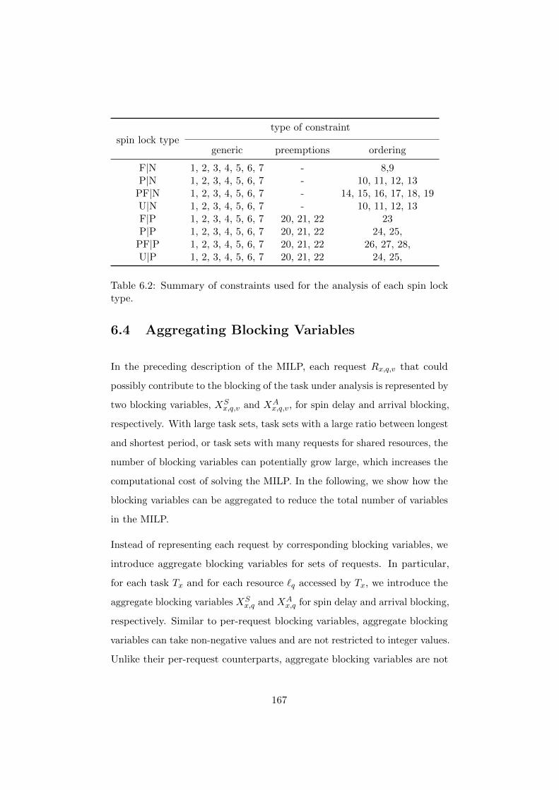
spin lock typetype of constraint
generic preemptions ordering
F|N 1, 2, 3, 4, 5, 6, 7 - 8,9P|N 1, 2, 3, 4, 5, 6, 7 - 10, 11, 12, 13
PF|N 1, 2, 3, 4, 5, 6, 7 - 14, 15, 16, 17, 18, 19U|N 1, 2, 3, 4, 5, 6, 7 - 10, 11, 12, 13F|P 1, 2, 3, 4, 5, 6, 7 20, 21, 22 23P|P 1, 2, 3, 4, 5, 6, 7 20, 21, 22 24, 25,
PF|P 1, 2, 3, 4, 5, 6, 7 20, 21, 22 26, 27, 28,U|P 1, 2, 3, 4, 5, 6, 7 20, 21, 22 24, 25,
Table 6.2: Summary of constraints used for the analysis of each spin locktype.
6.4 Aggregating Blocking Variables
In the preceding description of the MILP, each request Rx,q,v that could
possibly contribute to the blocking of the task under analysis is represented by
two blocking variables, XSx,q,v and XA
x,q,v, for spin delay and arrival blocking,
respectively. With large task sets, task sets with a large ratio between longest
and shortest period, or task sets with many requests for shared resources, the
number of blocking variables can potentially grow large, which increases the
computational cost of solving the MILP. In the following, we show how the
blocking variables can be aggregated to reduce the total number of variables
in the MILP.
Instead of representing each request by corresponding blocking variables, we
introduce aggregate blocking variables for sets of requests. In particular,
for each task Tx and for each resource `q accessed by Tx, we introduce the
aggregate blocking variables XSx,q and XA
x,q for spin delay and arrival blocking,
respectively. Similar to per-request blocking variables, aggregate blocking
variables can take non-negative values and are not restricted to integer values.
Unlike their per-request counterparts, aggregate blocking variables are not
167
generally upper-bounded by 1. The interpretation of the aggregate blocking
variables is similar to the interpretation of the per-request blocking variables:
in an arbitrary but fixed schedule, the requests for `q issued by jobs of Tx
contribute to Ji’s spin delay with exactly XSx,q ·Lx,q time units. The aggregate
blocking variables for arrival blocking are interpreted analogously.
The MILPs as described in the preceding sections can be rephrased such that
per-request blocking variables are avoided completely and aggregate blocking
variables are used instead. We illustrate this approach by constructing
the MILP for the analysis of F|N locks. Analogously to Equation (2), the
objective function for the MILP is to maximize
bi ,∑Tx∈τ i
∑`q∈Q
(XSx,q +XA
x,q
)· Lx,q. (14)
Note that this objective function stated with regard to aggregate blocking
variables is identical to the objective function we used previously when
applying the following substitution:
∀Tx ∈ τ i : ∀`q ∈ Q : XSx,q =
N ix,q∑
v=1
XSx,q,v and (15)
XAx,q =
N ix,q∑
v=1
XAx,q,v. (16)
In fact, as we will show, many constraints previously stated with regard
to per-request blocking variables can be rephrased for aggregate blocking
variables by applying the substitutions above. We next walk through all
constraints previously established for the analysis of F|N locks and detail
how they are adapted for aggregate blocking variables.
168
Constraint 1 is adapted as follows:
Constraint 29. In any schedule of τ :
∀Tx ∈ τ i : ∀`q ∈ Q : XAx,q +XS
x,q ≤ N ix,q.
Proof. Observe that jobs of Tx issue at most Nx,q requests for `q while a single
job of Ti is pending, and hence no more than N ix,q of Tx’s requests for `q can
cause Ji to incur arrival blocking or spin delay: XAx,q ≤ N i
x,q and XSx,q ≤ N i
x,q.
The remainder of the proof is identical to the proof of Constraint 1.
Constraints 2–4 do not contain any blocking variables and can be used un-
modified with aggregate blocking variables. Constraint 5 is simply adapted by
substituting per-request blocking variables according to Equation (16):
Constraint 30. In any schedule of τ :
∑Tx∈τ lh
∑`q
XAx,q ≤ 0. (17)
The proof is identical to the proof of Constraint 5. The remaining con-
straints applicable to F|N locks, Constraints 6–9, can similarly be adapted
by substituting the per-request blocking variables accordingly.
Constraint 31. In any schedule of τ :
∀`q ∈ Q :∑Tx∈τ ll
XAx,q ≤ Aq.
Proof. Suppose not. If Aq = 0, this would imply, by definition of XAx,q,
that in some schedule a request Rx,q,v caused Ji to incur arrival blocking,
even though by definition of Aq no request for `q arrival-blocked Ji, which is
clearly impossible. If Aq = 1, at least two requests by local lower-priority
169
tasks caused arrival blocking. Analogously to Constraint 2, this is impossible
because at most one request can be in progress on P (Ti) when Ji is released.
Constraint 32. In any schedule of τ :
∑Tx∈τ ll∪τ lh
∑`q
XSx,q ≤ 0. (18)
Proof. The proof is identical to the proof of Constraint 7.
Constraint 33. In any schedule of τ with F|N locks:
∀`q ∈ Q : ∀Pk, Pk 6= P (Ti) :∑
Tx∈τ(Pk)
XSx,q ≤ ncs(Ti, q).
Proof. The proof is identical to the proof of Constraint 8.
Constraint 34. In any schedule of τ with F|N locks:
∀Pk, Pk 6= P (Ti) : ∀`q ∈ Q :∑
Tx∈τ(Pk)
XAx,q ≤ Aq.
Proof. The proof is identical to the proof of Constraint 9.
Except for Constraint 29, all of the above constraints and the objective
function for F|N locks using aggregate blocking variables were obtained
by applying the respective substitutions (Equations (15) and (16)) for per-
request blocking variables, and hence, are equivalent with regard to the total
blocking they permit. Constraint 29, however, differs from the corresponding
170
constraint established using per-request blocking variables (Constraint 1). As
we will show, this does not introduce any pessimism when compared to the
analysis with per-request blocking variables presented in Section 6.3.2.
Theorem 5. The blocking bounds obtained from the analysis of F|N locks
using aggregate blocking variables does not exceed the blocking bounds
obtained from the analysis of F|N locks using per-request blocking variables.
Proof. We show that a solution to the MILP using aggregate blocking
variables can be transformed into a solution for the MILP with per-request
blocking variables that satisfies all constraints and has the same objective
value (i.e., blocking bound). Hence, the blocking bound obtained with the
MILP using aggregate blocking variables cannot exceed the blocking bound
obtained with the MILP with per-request blocking variables, as otherwise
the objective value would not be maximal.
Let τ be a task set and Ti with Ti ∈ τ the task under analysis. In the
following, we prefix all variables used in the formulation of the respective
MILPs with either ag or pr to denote that the variable is part of the MILP
using aggregate or per-request blocking variables, respectively. For instance,
we use prXSx,q,v to denote the blocking variable XS
x,q,v of the MILP using
per-request blocking variables, and we use agbi to denote Ti’s blocking bound
(i.e., objective value) obtained with the MILP using aggregate blocking
variables.
Let an assignment to the aggregate blocking variables agXSx,q and agX
Ax,q with
Tx ∈ τ i ∧ `q ∈ Q and the variables agAq with `q ∈ Q be given. We construct
an assignment to the variables prAq with `q ∈ Q as follows:
∀`q ∈ Q : prAq , agAq. (19)
171

We construct an assignment to the per-request blocking variables as fol-
lows:
∀Tx ∈ τ i : ∀`q ∈ Q : ∀v, 1 ≤ v ≤ N ix,q :
prXSx,q,v ,
1 if agX
Sx,q ≥ v
agXSx,q − bagXS
x,qc if v − 1 ≤ agXSx,q < v
0 if agXSx,q < v − 1
(20)
prXAx,q,v ,
agXAx,q if v = N i
x,q
0 if v 6= N ix,q.
(21)
The idea behind this construction is that the value assigned to one aggregate
blocking variable for spin delay is “distributed” among multiple per-request
blocking variables for spin delay, assigning a value of at most 1 to each
of them. The value of an aggregate blocking variable for arrival blocking
(which is at most 1) is directly assigned to one per-request blocking variable
for arrival blocking. As we show in the following, this construction ensures
that prbi = agbi holds and all constraints specified for the the MILP with
per-request blocking variables are satisfied.
Observe that this assignment by construction fulfills Equations (15) and (16)
that we previously used to substitute per-request blocking variables to obtain
constraints using aggregate blocking variables:
∀Tx ∈ τ i : ∀`q ∈ Q : agXSx,q =
N ix,q∑
v=1
prXSx,q,v (22)
agXAx,q =
N ix,q∑
v=1
prXAx,q,v. (23)
From the definition of the objective functions Equation (2) and Equation (14)
for the MILPs with per-request and aggregate blocking variables, respectively,
172

it directly follows that prbi = agbi holds. We next show that this assignment
also satisfies all constraints.
We start with Constraint 1 that we restate here for convenience:
∀Tx ∈ τ i : ∀`q ∈ Q : ∀v, 1 ≤ v ≤ N ix,q : prX
Ax,q,v + prX
Sx,q,v ≤ 1.
Let Tx with Tx ∈ τ i be a task and `q with `q ∈ Q be a resource. For blocking
variables prXSx,q,v and prX
Ax,q,v with v 6= N i
x,q, this follows immediately since
prXSx,q,v ≤ 1 by Equation (20) and prX
Ax,q,v = 0 by Equation (21). For
blocking variables with v = N ix,q, we distinguish between the three cases
considered in Equation (20). If agXSx,q = N i
x,q = v, then, by Constraint 33,
we have agXAx,q = 0, and hence prX
Sx,q,v = 1 and prX
Ax,q,v = 0, which satisfies
Constraint 1. If N ix,q − 1 ≤ agX
Sx,q < N i
x,q, then bagXSx,qc = N i
x,q − 1, and
hence, by Constraint 33, we have
XAx,q +XS
x,q ≤ N ix,q
XAx,q +XS
x,q − bagXSx,qc ≤ N i
x,q − bagXSx,qc
XAx,q +XS
x,q − bagXSx,qc ≤ 1.
It follows that Constraint 1 is satisfied. If agXSx,q < v − 1, Constraint 1
is trivially satisfied since agXAx,q ≤ agAq holds due to Constraints 30, 31,
and 34.
Constraints 2–4 trivially hold since these constraints are used unmodified for
the MILP with aggregate blocking variables. The assignment also trivially
satisfies Constraints 5–9: the corresponding Constraints 30–34 were obtained
by applying the substitution defined in Equations (15) and (16), and Equa-
tions (15) and (16) hold under the assignment defined in Equations (20)
and (21).
Hence, a solution to the MILP using aggregate blocking variables can be
173
transformed into a solution for the MILP using per-request blocking vari-
ables, and thus, the blocking bound obtained from the MILP using aggregate
blocking variables does not exceed the blocking bound obtained from the
MILP using per-request blocking variables.
As we show next, in the case of non-preemptable spin locks, the integer
variables used in the construction above can be eliminated, and hence, the
blocking analysis can be carried out by solving (non-integer) LPs.
6.5 Integer Relaxation
The MILP presented in this section for the analysis of non-preemptable spin
locks uses integer variables only for the binary decision variables Aq with
`q ∈ Q indicating whether a local request for `q can cause arrival blocking.
Since at most one of these variables can be set to 1 (by Constraint 2),
there exist only nr (recall that nr is defined as nr = |Q|) different feasible
assignments (one for each resource). These integer variables can be completely
eliminated by invoking the analysis for each possible assignment, where the
Aq variables are replaced with constants. The nr resulting (non-integer)
LPs are solved individually, and the highest objective value from any of
these constitutes the blocking bound. Importantly, this method of applying
our analysis using multiple (non-integer) LPs instead of one MILP does
not introduce any pessimism, but eliminates the need for integer or binary
variables.
For preemptable spin locks, our MILP formulation makes use of the additional
integer variables Cq with `q ∈ Q to denote the number of preemptions while
processing a request for `q. In contrast to the binary decision variables Aq,
the number of possible assignments to Cq variables (only constrained by
174
Constraints 21 and 22) can grow rapidly with the number of tasks. Hence,
invoking the analysis for each such assignment cannot be considered generally
practical. Instead, the integer requirement for Cq variables can be lifted to
obtain a (non-integer) LP. This relaxation can result in an increase of the
blocking bound in the order of at most O(nr) critical section lengths, which
follows from Constraint 21 limiting the sum of all Cq variables (regardless
whether integral or not), and the fact that any non-integral assignment to
any Cq variable differs by less than 1 from an integral one.
6.6 Analysis Accuracy and Computational Com-
plexity
6.6.1 Accuracy
In Section 6.2, we show that prior analysis approaches are inherently pes-
simistic due to execution time inflation. Our analysis, that we presented in
this chapter, eliminates this source of pessimism. Yet, our analysis cannot
be generally guaranteed to yield tight (i.e., exact) blocking bounds (except
for special cases, such as the case we describe in Section 7.3.3). This was
a deliberate choice: our goal was not to ensure tight blocking bounds, but
to devise a simple analysis approach that supports lock types for which no
prior analysis was available and improves upon prior techniques. Tightness
can potentially be achieved at the expense of an increased complexity of the
analysis approach. However, the development of a tight blocking analysis is
beyond the scope of this work.
Next, we consider the computational cost required by our analysis.
175
6.6.2 Computational Complexity
In contrast to prior analyses (e.g., the classic analysis of the MSRP summa-
rized in Section 2.5.1), our analysis approach makes use of “heavy machinery”,
namely MILP. As we argue in Section 6.5, in the case of non-preemptable
spin locks, integer variables can be eliminated by transforming the MILP
into a set of (non-integer) LPs. As we will show next, when using this
transformation, our blocking analysis of F|N locks can be carried out within
polynomial time.
Recall from Section 6.3 that our blocking analysis is used in conjunction
with a response-time analysis (Equation (1) in Section 6.3), similar to, for
instance, the classic MSRP analysis (where the response time analysis in
Equation (2.2) uses inflated execution times). Response-time analysis alone,
however, is already a (weakly) NP -hard problem [65], even without blocking
analysis. Therefore, we only consider the computational complexity of the
blocking analysis itself (i.e., generating and solving one MILP as described in
this chapter) in the following. We first consider F|N locks before discussing
the analysis complexity of the other lock types supported by our analysis
approach.
We begin by observing that our analysis uses only a polynomial number of
LPs for a single task.
Lemma 14. The elimination of integer variables in the generated MILP as
described in Section 6.5 results in a polynomial number of non-integer LPs
with respect to the size of the problem description (i.e., the list of tasks and
their critical sections).
Proof. Recall from Section 2.1.4 that each resource in Q is accessed at least
once, and hence, at least one critical section for each resource must be listed
in the problem description, which lower-bounds its size at Ω(n + nr) bits.
176
The claim follows since one LP is generated for each resource.
Each of the generated LPs is of polynomial size.
Lemma 15. Each generated LP used for the analysis of F|N locks is of
polynomial size with respect to the size of the problem description.
Proof. By construction, per task and resource, two (aggregate) blocking
variables (for spin delay and arrival blocking) are used, resulting in O(n ·
nr) blocking variables in total. Further, by construction, for each type of
constraint, O(n · nr) individual constraints (one for each resource and task)
are generated.
Since the size of the problem description is lower-bounded by Ω(n+ nr) and
the number of constraints and variables are each polynomial with respect to
the size of the problem description, it follows that each LP is of polynomial
size with respect to the size of the problem description.
Generating each constraint in the LP only takes polynomial time.
Lemma 16. Any single constraint for the analysis of F|N locks can be
generated within polynomial time with respect to the size of the problem
description.
Proof. Recall from Section 2.1 that the task set and the set of resources
are represented as sets (rather than, for instance, just the number thereof).
Iterating over the set of tasks and resources, as we do for the construction
of the constraints, takes linearly many steps with respect to the size of the
respective sets. Further, the set operations (e.g., τ(Pk)) and functions (e.g.,
ncs(Ti, q)) summarized in Table 6.1 used for constructing the constraints for
F|N locks can all be carried out within strictly polynomial time with respect
to the size of the problem description. The claim follows.
177
Since each LP is of polynomial size, and generating each constraint takes
only polynomial time, each LP can be generated within polynomial time as
well.
Finally, we can conclude that the analysis of F|N locks can be carried out
within polynomial time.
Lemma 17. The blocking analysis of F|N for a single task can be carried out
within polynomial time with respect to the size of the problem description.
Proof. Follows from the preceding lemmas. For the analysis of a single task, a
polynomial number of LPs are generated within polynomial time, where each
LP is of polynomial size. Further, each LP can be solved within polynomial
time [78, 88]. The claim follows.
The analysis of F|P locks makes use of additional nr integer variables (Cq).
When these variables are relaxed (at the cost of potentially increased pes-
simism), the previous argument applies and the analysis of F|P can be carried
out within polynomial time as well.
Although the size of the LPs for the analysis of the remaining lock types (i.e.,
U|*, P|*, and PF|* locks) is polynomial as well, the cost of generating the
LPs differs from the cost of generating the LPs for F|* locks in one crucial
aspect: for each lock type with priority-ordering (or no guaranteed ordering)
we use per-request wait-time bounds to obtain the constraints for the LP
(e.g., Constraint 10 for P|N locks). We compute these wait-time bounds
by solving a recurrence (e.g., Equation (3) for P|N locks) via fixed-point
iteration, similar to response-time analysis for fixed-priority scheduling. In
the case of response-time analysis, it has been shown that the response-time
cannot be computed within polynomial time (unless P = NP) [65], and hence,
it is unlikely that wait-time bounds can be computed within polynomial
178
time. However, since we have a stop criterion in the fixed-point iteration, the
time for computing the wait-time bounds is pseudo-polynomially bounded
in the period of each task: the fixed-point iteration is aborted if no fixed
point smaller than or equal to the period of the task is found. Hence, in each
iteration, the preliminary value of the wait-time bound is either increased by
at least 1 (recall from Section 2.1.1 that we assume discrete time), or a fixed
point is found. Hence, the number of steps taken in the fixed-point iteration
process is pseudo-polynomially bounded by the task’s period. Except for the
computation of the wait-time bounds, the generation and solving of the LPs
for the analysis of U|*, P|*, and PF|* locks is polynomial with respect to
the input size, similar to the LPs for F|* locks. To summarize, overall the
analysis for U|*, P|*, and PF|* locks takes pseudo-polynomial time. If the
constraints using wait-time bounds are omitted (at the cost of potentially
increased pessimism), the analysis can be carried out within polynomial time
as well.
Next, we present the results of a large-scale experimental evaluation, where
we investigated the impact of the different spin locks types and analyses in a
broad range of different scenarios.
6.7 Evaluation
We conducted a large-scale experimental evaluation comparing all considered
spin lock types and analyses (where available) to answer the following key
questions:
Q1: Does our blocking analysis approach yield less pessimistic blocking
bounds than prior analysis techniques, and hence, higher task set
schedulability?
Q2: Can we identify a spin lock type that is a reasonable default choice?
179
Q3: Are the dominance relations between spin lock types reflected in schedu-
lability results?
To answer these questions, we implemented our analysis approach as described
above, and we performed a large-scale experimental evaluation in a variety
of different settings.
6.7.1 Implementation
We implemented our analysis as part of the SchedCAT open-source project [10].
Similar to other analyses and functionality in SchedCAT, we primarily used
Python as programming language, but computationally intensive parts of
our analysis were implemented using C++ to avoid performance bottle-
necks. For solving the generated MILPs, we made use of the GNU Linear
Programming Kit (GLPK) [75]. We did not eliminate or relax the (few)
integer variables in our MILP formulation (see Section 6.5) to obtain pure
(non-integer) LPs.
6.7.2 Experimental Setup
For our experimental evaluation, we considered a broad range of different
settings: we varied the number of processor cores in the system, the task
set characteristics, the number of shared resources, and the way they are
accessed by the tasks. A summary of the parameter ranges we explored in
our evaluation is given in Table 6.3. To start with, we considered systems
with 4, 8 and 16 cores. Embedded systems with 4 and 8 cores are readily
available today, whereas embedded platforms with 16 cores are a slightly more
forward-looking scenario. We generated task sets with up to 10 tasks per
core (i.e., n ∈ m, 2m, . . . , 10m) using the task set generator presented by
Emberson et al . [68]. Task periods were chosen at random from the interval
180
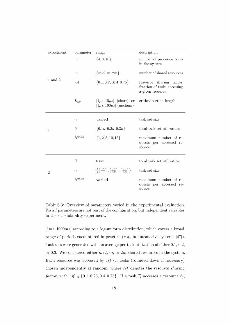
experiment parameter range description
1 and 2
m 4, 8, 16 number of processor coresin the system
nr m/2,m, 2m number of shared resources
rsf 0.1, 0.25, 0.4, 0.75 resource sharing factor:fraction of tasks accessinga given resource
Li,q [1µs, 15µs] (short) or[1µs, 100µs] (medium)
critical section length
1
n varied task set size
U 0.1n, 0.2n, 0.3n total task set utilization
Nmax 1, 2, 5, 10, 15 maximum number of re-quests per accessed re-source
2
U 0.5m total task set utilization
n⌈
U0.1
⌉,⌈
U0.2
⌉,⌈
U0.3
⌉task set size
Nmax varied maximum number of re-quests per accessed re-source
Table 6.3: Overview of parameters varied in the experimental evaluation.Varied parameters are not part of the configuration, but independent variablesin the schedulability experiment.
[1ms, 1000ms] according to a log-uniform distribution, which covers a broad
range of periods encountered in practice (e.g., in automotive systems [47]).
Task sets were generated with an average per-task utilization of either 0.1, 0.2,
or 0.3. We considered either m/2, m, or 2m shared resources in the system.
Each resource was accessed by rsf · n tasks (rounded down if necessary)
chosen independently at random, where rsf denotes the resource sharing
factor, with rsf ∈ 0.1, 0.25, 0.4, 0.75. If a task Ti accesses a resource `q,
181
then the number of Ti’s requests for `q (i.e., Ni,q) was chosen at randomly
from the interval [1, . . . , Nmax]. The maximum number of requests Nmax
was set to one of 1, 2, 5, 10, 15. The critical section length Li,q was chosen
at random either from the short interval [1µs, 15µs] or the medium interval
[1µs, 100µs]. In the following, we denote a concrete combination of the above
parameters as a configuration. We enforced that the cumulative length of all
requests issued by a single task does not exceed its execution time. Formally:
∀Ti ∈ τ : ei ≥∑
`q∈Q Li,q ·Ni,q.
For the lock types that support request priorities (i.e., P|N, P|P, PF|N, and
PF|P), we employed a straightforward scheme for assigning these priorities:
Initially, all tasks are assigned the same (lowest) request priority. If a task set
cannot be determined to be schedulable, the request priority of the tasks that
cannot be shown to meet their deadlines is iteratively increased. This step is
repeated until either the task set becomes schedulable or one of the following
conditions apply: the task that cannot be shown to meet its deadline already
has the highest locking priority, the locking priority of the same task has been
already increased in the previous step, locking priorities are increased only
for a small subset of the tasks in an alternating fashion over the last couple of
steps. In either of these cases, further locking priority increases are deemed
ineffective and schedulability cannot be established. Note that we assign the
same priority to all requests issued by the same task (which is independent
from its scheduling priority). Yet, our analysis supports assigning more
fine-grained priorities at the level of resources (i.e., per task and per accessed
resource). However, the development of a more sophisticated scheme for
assigning request priorities (possibly at finer granularity than per task) is
beyond the scope of this work.
We studied the schedulability in two sets of experiments to measure the
impact of either varying system load or varying lock contention. In particular,
in the first set of experiments, all parameters of a configuration were fixed,
182
and the schedulability was measured as a function of the task set size. In
the second set of experiments, the total utilization was fixed to U = m/2,
and the task set size was determined by the average task utilization of
the configuration (rounding up if necessary). The schedulability was then
measured as a function of the maximum number of requests Nmax, which
we varied across the interval [1, 40].
For each configuration, we generated and tested at least 1000 sample task
sets for each n (in the first set of experiments) or Nmax (in the second set
of experiments). In both sets of experiments, we applied eleven blocking
analyses in total: the MILP-based analysis for each of the considered spin
lock type (presented above), Gai et al .’s classic [72] (labeled “MSRP-classic”)
and Brandenburg’s holistic [43, Ch. 5] analysis (labeled “MSRP-holistic”)
for F|N spin locks. Finally, we added results for the (hypothetical) case
in which no blocking occurs (labelled “no blocking”), that is, resources are
treated as private rather than shared, and tasks are considered to execute
independently. These results serve as an upper bound on schedulability (as
schedulability can only decrease when accounting for blocking effects).
In the interest of performance, we did not unconditionally apply all analyses
to each task set. In the case of F|N, we first applied —the comparably cheap—
holistic analysis, and used our —less pessimistic but computationally more
demanding— analysis for F|N locks only when the holistic analysis did not
already establish schedulability. Similarly, since F|N locks can be treated
as a special case of PF|N locks with all request priorities set to the same
value (see Section 5.6, we apply our analysis for PF|N only if the task set
was not already established to be schedulable with F|N locks (either using
our analysis for F|N locks or the holistic analysis). We performed similar
optimizations for preemptable spin locks. Note that these optimizations do
not affect the experimental results, but only their computational cost.
183
Next, we highlight trends and key findings from the experimental results.
Due to the large number of considered configurations, we illustrate our
observations with selected representative configurations. The full results can
be found online [132].
6.7.3 Experimental Results
First, we made the —not entirely unexpected— observation that, if blocking
effects are not the “bottleneck” of a task set determining its schedulability,
for instance in cases of low resource contention, then the choice of spin lock
type has little impact. An example for such a configuration is shown in
Figure 6.4, where schedulability is close to the no-blocking case regardless of
the spin lock type or analysis. However, as shown in Figures 6.5 and 6.6 (and
most other results presented here), even with moderate resource contention,
significant differences in terms of schedulability can be observed as the system
load or the number of critical sections increases.
Second, we found that the schedulability results from both sets of experiments,
where we varied either load or contention, exhibit largely similar patterns
and trends. Hence, unless specified otherwise, the following observations
apply to both sets of experiments.
Comparison with Prior Analyses
Figure 6.5 depicts the schedulability for varying load in a case representative
for a broad range of configurations. Here, the holistic analysis of F|N
locks (labeled “MSRP-holistic”) results in slightly higher schedulability than
Gai et al .’s classic MSRP analysis (labeled “MSRP-classic”), which can
be attributed to a decrease of pessimism in the holistic analysis. Similar
observations can be made when varying contention, for instance, in the
184

0
0.2
0.4
0.6
0.8
1
8 10 12 14 16 18 20 22 24 26
schedula
ble
number of tasks
MSRP-classicMSRP-holistic
F|NU|NP|N
PF|Nno blocking
(a) Non-preemptable spin locks.
0
0.2
0.4
0.6
0.8
1
8 10 12 14 16 18 20 22 24 26
schedula
ble
number of tasks
F|PU|PP|P
PF|Pno blocking
(b) Preemptable spin locks.
Figure 6.4: Schedulability for m = 8, U = 0.3n, 4 shared resources, rsf =0.40, Nmax = 2, and short critical sections.
schedulability results depicted in Figure 6.6.
Under our analysis of F|N locks, the schedulability is further increased: in
the scenario depicted in Figure 6.5, more than ten additional tasks can
be supported on the same platform (or approximately 4 additional critical
sections in Figure 6.6). This increase in schedulability under our analysis
can be observed for a wide range of different configurations, which highlights
the typically less pessimistic nature inherent in our approach.
This decrease in pessimism under our analysis is further substantiated when
comparing the schedulability results under the the prior MSRP analyses
185
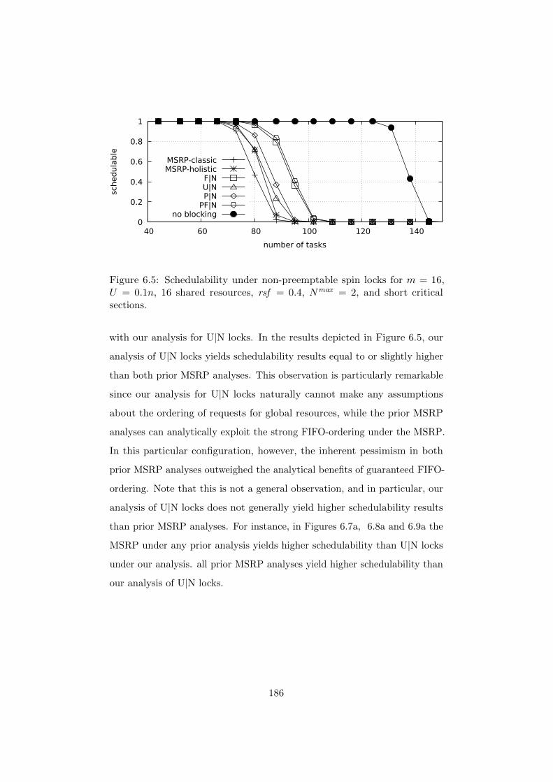
0
0.2
0.4
0.6
0.8
1
40 60 80 100 120 140
sched
ula
ble
number of tasks
MSRP-classicMSRP-holistic
F|NU|NP|N
PF|Nno blocking
Figure 6.5: Schedulability under non-preemptable spin locks for m = 16,U = 0.1n, 16 shared resources, rsf = 0.4, Nmax = 2, and short criticalsections.
with our analysis for U|N locks. In the results depicted in Figure 6.5, our
analysis of U|N locks yields schedulability results equal to or slightly higher
than both prior MSRP analyses. This observation is particularly remarkable
since our analysis for U|N locks naturally cannot make any assumptions
about the ordering of requests for global resources, while the prior MSRP
analyses can analytically exploit the strong FIFO-ordering under the MSRP.
In this particular configuration, however, the inherent pessimism in both
prior MSRP analyses outweighed the analytical benefits of guaranteed FIFO-
ordering. Note that this is not a general observation, and in particular, our
analysis of U|N locks does not generally yield higher schedulability results
than prior MSRP analyses. For instance, in Figures 6.7a, 6.8a and 6.9a the
MSRP under any prior analysis yields higher schedulability than U|N locks
under our analysis. all prior MSRP analyses yield higher schedulability than
our analysis of U|N locks.
186
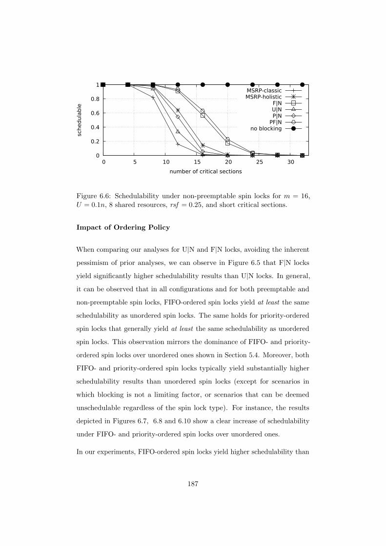
0
0.2
0.4
0.6
0.8
1
0 5 10 15 20 25 30
schedula
ble
number of critical sections
MSRP-classicMSRP-holistic
F|NU|NP|N
PF|Nno blocking
Figure 6.6: Schedulability under non-preemptable spin locks for m = 16,U = 0.1n, 8 shared resources, rsf = 0.25, and short critical sections.
Impact of Ordering Policy
When comparing our analyses for U|N and F|N locks, avoiding the inherent
pessimism of prior analyses, we can observe in Figure 6.5 that F|N locks
yield significantly higher schedulability results than U|N locks. In general,
it can be observed that in all configurations and for both preemptable and
non-preemptable spin locks, FIFO-ordered spin locks yield at least the same
schedulability as unordered spin locks. The same holds for priority-ordered
spin locks that generally yield at least the same schedulability as unordered
spin locks. This observation mirrors the dominance of FIFO- and priority-
ordered spin locks over unordered ones shown in Section 5.4. Moreover, both
FIFO- and priority-ordered spin locks typically yield substantially higher
schedulability results than unordered spin locks (except for scenarios in
which blocking is not a limiting factor, or scenarios that can be deemed
unschedulable regardless of the spin lock type). For instance, the results
depicted in Figures 6.7, 6.8 and 6.10 show a clear increase of schedulability
under FIFO- and priority-ordered spin locks over unordered ones.
In our experiments, FIFO-ordered spin locks yield higher schedulability than
187
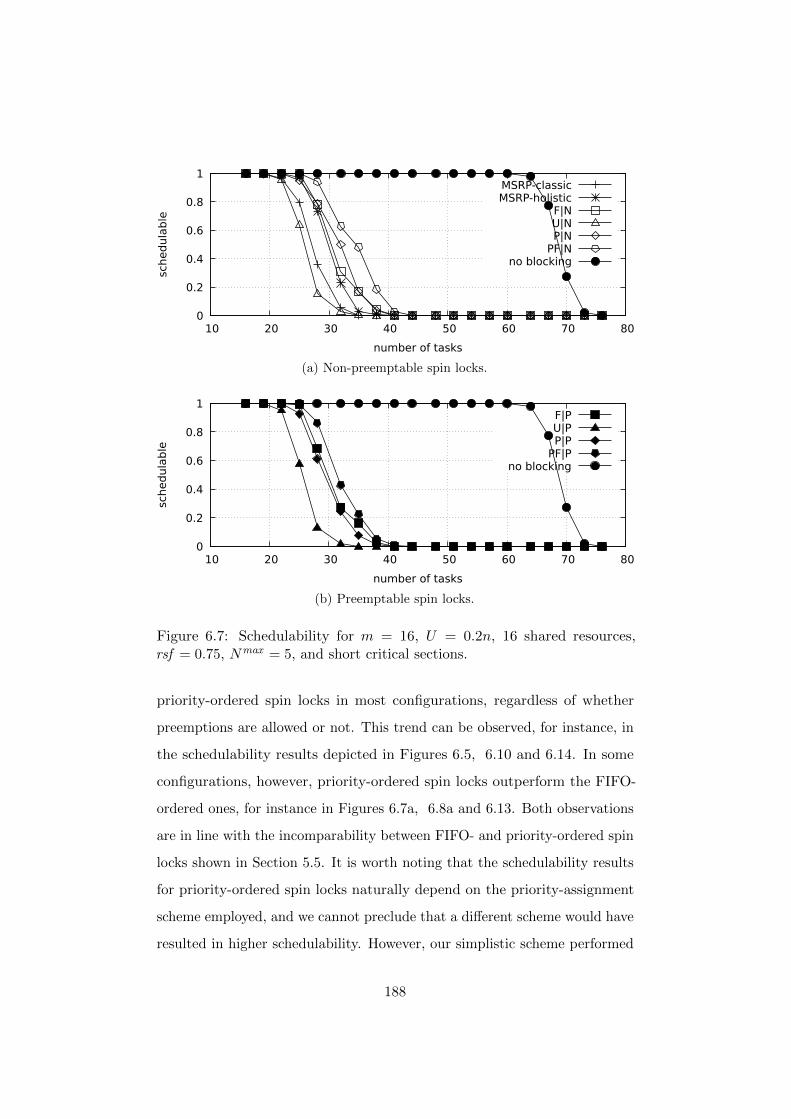
0
0.2
0.4
0.6
0.8
1
10 20 30 40 50 60 70 80
schedula
ble
number of tasks
MSRP-classicMSRP-holistic
F|NU|NP|N
PF|Nno blocking
(a) Non-preemptable spin locks.
0
0.2
0.4
0.6
0.8
1
10 20 30 40 50 60 70 80
schedula
ble
number of tasks
F|PU|PP|P
PF|Pno blocking
(b) Preemptable spin locks.
Figure 6.7: Schedulability for m = 16, U = 0.2n, 16 shared resources,rsf = 0.75, Nmax = 5, and short critical sections.
priority-ordered spin locks in most configurations, regardless of whether
preemptions are allowed or not. This trend can be observed, for instance, in
the schedulability results depicted in Figures 6.5, 6.10 and 6.14. In some
configurations, however, priority-ordered spin locks outperform the FIFO-
ordered ones, for instance in Figures 6.7a, 6.8a and 6.13. Both observations
are in line with the incomparability between FIFO- and priority-ordered spin
locks shown in Section 5.5. It is worth noting that the schedulability results
for priority-ordered spin locks naturally depend on the priority-assignment
scheme employed, and we cannot preclude that a different scheme would have
resulted in higher schedulability. However, our simplistic scheme performed
188
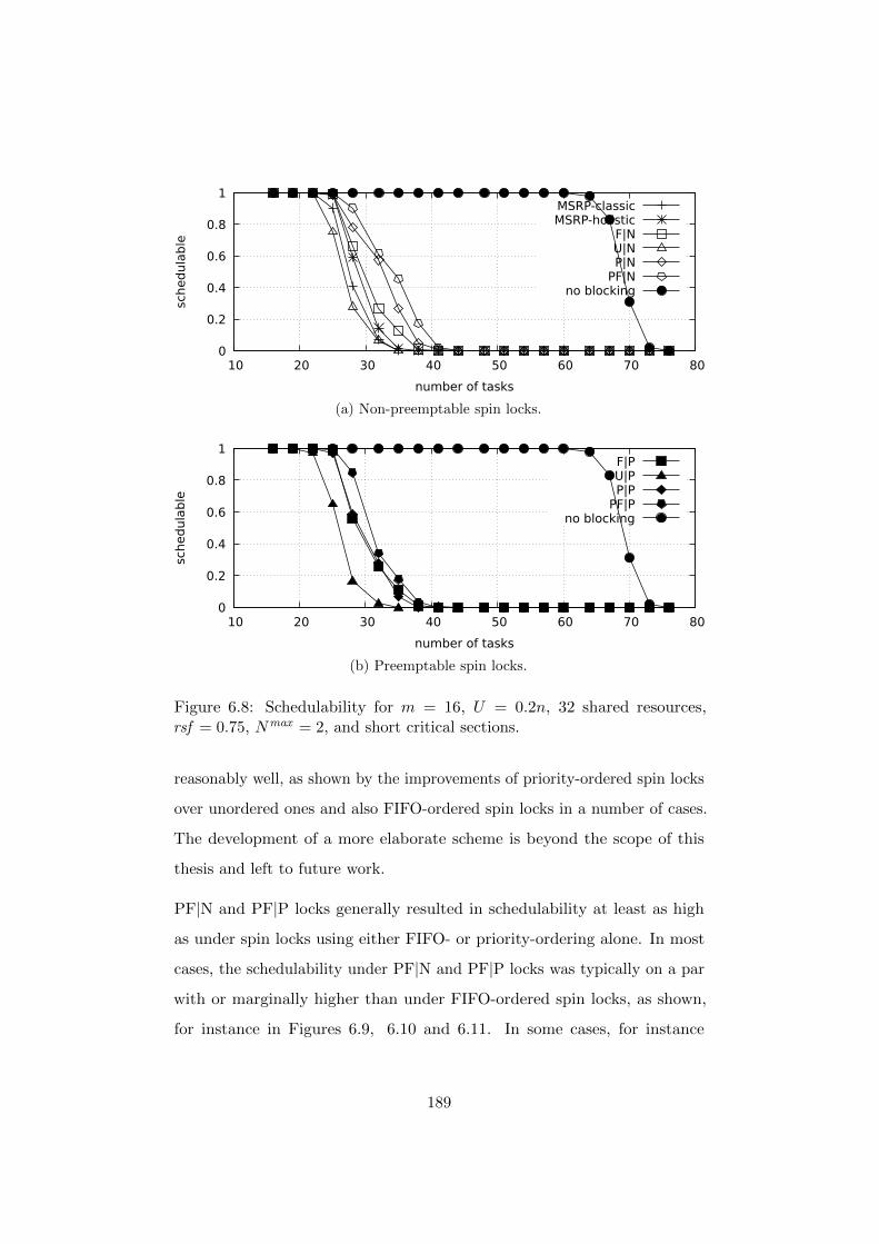
0
0.2
0.4
0.6
0.8
1
10 20 30 40 50 60 70 80
schedula
ble
number of tasks
MSRP-classicMSRP-holistic
F|NU|NP|N
PF|Nno blocking
(a) Non-preemptable spin locks.
0
0.2
0.4
0.6
0.8
1
10 20 30 40 50 60 70 80
schedula
ble
number of tasks
F|PU|PP|P
PF|Pno blocking
(b) Preemptable spin locks.
Figure 6.8: Schedulability for m = 16, U = 0.2n, 32 shared resources,rsf = 0.75, Nmax = 2, and short critical sections.
reasonably well, as shown by the improvements of priority-ordered spin locks
over unordered ones and also FIFO-ordered spin locks in a number of cases.
The development of a more elaborate scheme is beyond the scope of this
thesis and left to future work.
PF|N and PF|P locks generally resulted in schedulability at least as high
as under spin locks using either FIFO- or priority-ordering alone. In most
cases, the schedulability under PF|N and PF|P locks was typically on a par
with or marginally higher than under FIFO-ordered spin locks, as shown,
for instance in Figures 6.9, 6.10 and 6.11. In some cases, for instance
189
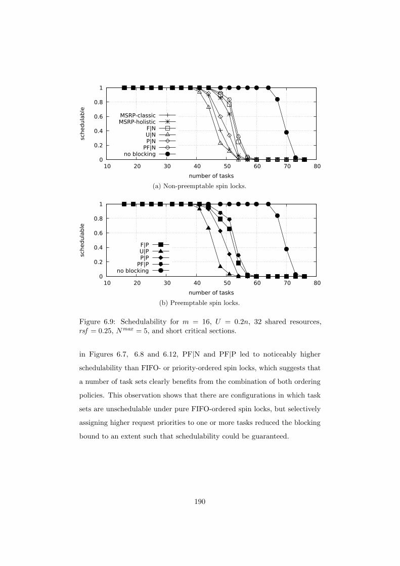
0
0.2
0.4
0.6
0.8
1
10 20 30 40 50 60 70 80
schedula
ble
number of tasks
MSRP-classicMSRP-holistic
F|NU|NP|N
PF|Nno blocking
(a) Non-preemptable spin locks.
0
0.2
0.4
0.6
0.8
1
10 20 30 40 50 60 70 80
schedula
ble
number of tasks
F|PU|PP|P
PF|Pno blocking
(b) Preemptable spin locks.
Figure 6.9: Schedulability for m = 16, U = 0.2n, 32 shared resources,rsf = 0.25, Nmax = 5, and short critical sections.
in Figures 6.7, 6.8 and 6.12, PF|N and PF|P led to noticeably higher
schedulability than FIFO- or priority-ordered spin locks, which suggests that
a number of task sets clearly benefits from the combination of both ordering
policies. This observation shows that there are configurations in which task
sets are unschedulable under pure FIFO-ordered spin locks, but selectively
assigning higher request priorities to one or more tasks reduced the blocking
bound to an extent such that schedulability could be guaranteed.
190
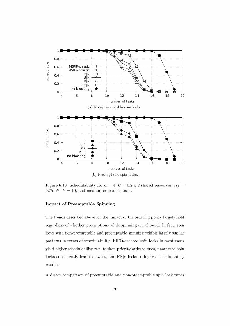
0
0.2
0.4
0.6
0.8
1
4 6 8 10 12 14 16 18 20
schedula
ble
number of tasks
MSRP-classicMSRP-holistic
F|NU|NP|N
PF|Nno blocking
(a) Non-preemptable spin locks.
0
0.2
0.4
0.6
0.8
1
4 6 8 10 12 14 16 18 20
schedula
ble
number of tasks
F|PU|PP|P
PF|Pno blocking
(b) Preemptable spin locks.
Figure 6.10: Schedulability for m = 4, U = 0.2n, 2 shared resources, rsf =0.75, Nmax = 10, and medium critical sections.
Impact of Preemptable Spinning
The trends described above for the impact of the ordering policy largely hold
regardless of whether preemptions while spinning are allowed. In fact, spin
locks with non-preemptable and preemptable spinning exhibit largely similar
patterns in terms of schedulability: FIFO-ordered spin locks in most cases
yield higher schedulability results than priority-ordered ones, unordered spin
locks consistently lead to lowest, and FN|∗ locks to highest schedulability
results.
A direct comparison of preemptable and non-preemptable spin lock types
191
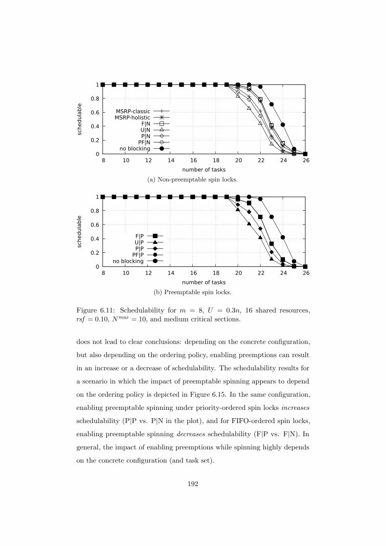
0
0.2
0.4
0.6
0.8
1
8 10 12 14 16 18 20 22 24 26
schedula
ble
number of tasks
MSRP-classicMSRP-holistic
F|NU|NP|N
PF|Nno blocking
(a) Non-preemptable spin locks.
0
0.2
0.4
0.6
0.8
1
8 10 12 14 16 18 20 22 24 26
schedula
ble
number of tasks
F|PU|PP|P
PF|Pno blocking
(b) Preemptable spin locks.
Figure 6.11: Schedulability for m = 8, U = 0.3n, 16 shared resources,rsf = 0.10, Nmax = 10, and medium critical sections.
does not lead to clear conclusions: depending on the concrete configuration,
but also depending on the ordering policy, enabling preemptions can result
in an increase or a decrease of schedulability. The schedulability results for
a scenario in which the impact of preemptable spinning appears to depend
on the ordering policy is depicted in Figure 6.15. In the same configuration,
enabling preemptable spinning under priority-ordered spin locks increases
schedulability (P|P vs. P|N in the plot), and for FIFO-ordered spin locks,
enabling preemptable spinning decreases schedulability (F|P vs. F|N). In
general, the impact of enabling preemptions while spinning highly depends
on the concrete configuration (and task set).
192

0
0.2
0.4
0.6
0.8
1
15 20 25 30 35 40 45 50 55
schedula
ble
number of tasks
MSRP-classicMSRP-holistic
F|NU|NP|N
PF|Nno blocking
(a) Non-preemptable spin locks.
0
0.2
0.4
0.6
0.8
1
15 20 25 30 35 40 45 50 55
schedula
ble
number of tasks
F|PU|PP|P
PF|Pno blocking
(b) Preemptable spin locks.
Figure 6.12: Schedulability for m = 16, U = 0.3n, 32 shared resources,rsf = 0.40, Nmax = 1, and short critical sections.
6.7.4 Summary of Experimental Results
Our first objective of the experimental evaluation was to study whether
the reduction of pessimism in our blocking analysis approach compared to
prior spin locks analysis techniques results in higher schedulability. For F|N
locks, for which prior analyses are available, our evaluation results show
increased schedulability (often by a significant margin) under our analysis
over a wide range of different configurations. The schedulability results
depicted in Figures 6.5 and 6.6 illustrate this result for two representative
configurations.
193

0
0.2
0.4
0.6
0.8
1
15 20 25 30 35 40 45 50 55
schedula
ble
number of tasks
MSRP-classicMSRP-holistic
F|NU|NP|N
PF|Nno blocking
(a) Non-preemptable spin locks.
0
0.2
0.4
0.6
0.8
1
15 20 25 30 35 40 45 50 55
schedula
ble
number of tasks
F|PU|PP|P
PF|Pno blocking
(b) Preemptable spin locks.
Figure 6.13: Schedulability for m = 16, U = 0.3n, 32 shared resources,rsf = 0.75, Nmax = 1, and short critical sections.
In our experiments, FIFO-ordered spin locks typically led to higher schedu-
lability results than priority-ordered spin locks, although priority-ordering
appears to be preferable in a number of configurations. Highest schedulability
results are achieved with either PF|N and PF|P locks, but the improvements
over FIFO-ordered spin locks (if any) are typically marginal. Our results
on the impact of allowing preemptions while spinning do not exhibit a clear
trend favoring either of these options. Unordered spin locks consistently led
to the lowest schedulability results, which highlights the importance of strong
ordering guarantees to bound worst-case behavior. However, our results also
show that unordered spin locks are “good enough” in a range of scenarios
194
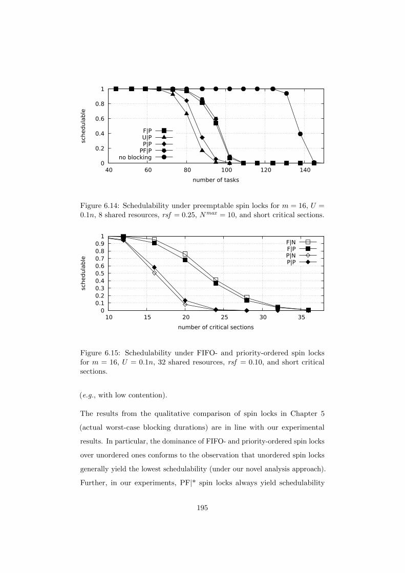
0
0.2
0.4
0.6
0.8
1
40 60 80 100 120 140
schedula
ble
number of tasks
F|PU|PP|P
PF|Pno blocking
Figure 6.14: Schedulability under preemptable spin locks for m = 16, U =0.1n, 8 shared resources, rsf = 0.25, Nmax = 10, and short critical sections.
0 0.1 0.2 0.3 0.4 0.5 0.6 0.7 0.8 0.9
1
10 15 20 25 30 35
schedula
ble
number of critical sections
F|NF|PP|NP|P
Figure 6.15: Schedulability under FIFO- and priority-ordered spin locksfor m = 16, U = 0.1n, 32 shared resources, rsf = 0.10, and short criticalsections.
(e.g., with low contention).
The results from the qualitative comparison of spin locks in Chapter 5
(actual worst-case blocking durations) are in line with our experimental
results. In particular, the dominance of FIFO- and priority-ordered spin locks
over unordered ones conforms to the observation that unordered spin locks
generally yield the lowest schedulability (under our novel analysis approach).
Further, in our experiments, PF|* spin locks always yield schedulability
195

results at least as high as FIFO- or priority-ordered spin lock, which is in line
with the dominance of PF|* spin locks over both FIFO- and priority-ordered
spin locks.
6.8 Summary
We presented a novel blocking analysis approach for P-FP systems supporting
eight different types of spin locks, most of which were not supported by prior
analyses. Notably, we provided an analysis for unordered spin locks that
can be safely used even if the ordering policy of a spin lock is not known
(e.g., AUTOSAR mandates spin locks, but does not specify a particular
type).
One important aspect of our approach is that the objective function of
the MILP maximizes the blocking, and the constraints can only reduce the
objective value (i.e., blocking bound). Constraints can be proven individually
and the soundness of the analysis follows from the soundness of the individual
constraints. Crucially, the soundness of the analysis does not depend on
whether any particular set of constraints is imposed, but rather only on
whether the constraints used are correct. In fact, omitting some of the
presented constraints (or even all of them) will still yield sound (albeit likely
more pessimistic) results.
The primary aim of our approach was to support a range of spin lock types
not supported in prior work and to eliminate the pessimism inherent in prior
analyses. Although our approach is asymptotically less pessimistic than prior
analyses (where available), it cannot be guaranteed to yield tight blocking
bounds (except for special cases, see Section 7.3.3). Moreover, we do not
claim the set of constraints presented to be complete, in the sense that it
may be possible to find additional constraints to further reduce analysis
196

pessimism.
Despite not necessarily being tight, the results of a large-scale experimental
evaluation covering a broad range of different scenarios show that our analysis
commonly yields improved—often by a significant margin—schedulability
compared to prior analyses.
The evaluation results also allow for a comparison of the different spin lock
types on a common basis. Based on our results, we suggest four improvements
to the support of spin locks in AUTOSAR:
1. AUTOSAR should specify the concrete type of spin lock. Not specify-
ing the spin lock type requires making safe, but pessimistic assumptions
for analyzing the system (e.g., assuming unordered spin locks), nega-
tively impacting schedulability.
2. AUTOSAR should specify support for FIFO-ordered spin locks. Our
evaluation results show that FIFO-ordered spin locks (together with
PF|* locks) typically yield the highest schedulability results over a wide
range of different scenarios. In addition,
3. AUTOSAR should specify support for priority-ordered spin locks,
since there exist workloads supported by priority-ordered spin locks,
but not FIFO-ordering alone. Importantly, request-priorities should be
configurable independently of scheduling priorities.
4. Strong ordering guarantees can reduce worst-case blocking and allow-
ing preemptions while spinning may be required by latency-sensitive
applications. The AUTOSAR API for spin locks should hence be
extended to explicitly support preemptable spinning without sacrificing
ordering guarantees as we point out in Section 2.4.2.
Note that we suggested that AUTOSAR should specify support for FIFO-
and priority-ordered spin locks, but not PF|N or PF|P locks although they
197

achieved consistently highest schedulability in our experimental evaluation.
The reason is that PF|N or PF|P typically offer only marginal (if any) benefits
over pure FIFO- or priority-ordered spin locks, and potentially introduce ad-
ditional implementation and runtime overhead — both undesirable properties
in resource-constrained embedded systems.
The blocking analysis presented in this chapter does not support nested
requests. Lifting this restriction while maintaining the same accuracy in-
herently increases the computational complexity of the blocking analysis
problem, as we show in the next chapter.
198
Chapter 7
Analysis Complexity of
Nested Locks1
7.1 Introduction
In the previous chapters, we assumed that lock requests are not nested, that
is, at any time, a job can hold at most one lock. Nesting of requests, however,
can be desirable for performance reasons (e.g., to enable fine-grained locking
in shared data structures), or may even be an implicit effect of modularization
in sufficiently large software stacks (e.g., calls to library functions or system
calls can involve lock acquisitions, and hence nesting of requests).
Extending our blocking analysis presented in the previous chapter to nested
spin locks seemed a natural next step, but posed significant challenges,
especially maintaining reasonably low computational cost2 while accounting
for new blocking effects enabled by nesting. In fact, as we show in this
chapter by reductions from a matching problem, the decision variant of
1This chapter is based on [134].2Polynomial runtime for F|N locks, see Section 6.6.2.
199
the blocking analysis problem for nested spin locks with FIFO- or priority-
ordering is strongly NP -hard.3 Our results are rather general and not limited
to spin locks: the reductions do not rely on the scheduler (as long as it is
work-conserving), whether preemptions are allowed, and whether blocked
jobs spin or suspend. Our hardness results hence generally hold for mutex
locks and are not specific to spin locks.
Perhaps surprisingly, in a special case in which the blocking analysis problem
for FIFO- and priority-ordered locks is strongly NP -hard, we found that the
analysis for unordered locks with nesting can be carried out within polynomial
time. In that sense, strong ordering guarantees appear to be a double-edged
sword when it comes to blocking and its analysis: without nesting, both
FIFO- and priority-ordering can be efficiently exploited analytically (see
Section 6.3), and result in higher schedulability (see Section 6.7). Nested
locks with strong ordering guarantees, however, do not lend themselves to
an efficient analysis. At the same time, the analysis of unordered locks,
under the same assumptions we make for our reductions, can be framed as a
computationally inexpensive graph reachability problem.
The difficulty of the blocking analysis problem for nested locks arises from
blocking effects not present under non-nested locks. We describe such effects
next.
7.2 Blocking Effects with Nested Locks
Without nesting, two requests Rx,q,v and Ry,p,w can potentially block each
other if they were issued from different processors (P (Tx) 6= P (Ty)) and both
access the same resource (q = p). Importantly, whether Rx,q,v and Ry,p,w
3In the following, we refer to the decision variant of the blocking analysis problem (seeSection 7.3.3) when stating NP-hardness of the blocking analysis problem.
200

can block each other can be determined regardless of requests issued from
other processors (other than P (Tx) and P (Ty)). With nesting, in contrast,
a request can also be transitively blocked by another request for a different
resource. At the same time, certain requests from different processors for the
same resource cannot block each other when guarded by other requests.
7.2.1 Transitive Nested Blocking
While under non-nested locks a request can only be blocked by other requests
for the same resource, nesting blurs this picture and enables scenarios in
which even requests for different resources contribute to blocking, and hence
have to be accounted for. Figure 7.1a depicts a schedule illustrating this
effect. In this scenario, three jobs, Ji, Jx, and Jy, are each assigned to their
own processor. Job Ji issues a single request for `1, Jx issues a request for
`1 that contains a nested request for `2, and Jy issues one request for `2.
Figure 7.1b depicts the requests issued and the blocking effects incurred by
these jobs. Ji’s request for `1 is blocked by Jx’s request for `1. In turn, Jx’s
request for `2 nested within the request for `1 is blocked by Jy’s request for
`2. As a result, Ji’s request is transitively blocked by Jy’s request, although
Ji and Jy access different resources — an effect impossible under non-nested
locks.
Without nesting, transitive nested blocking of requests for different resources
is not possible. Nesting, however, also prevents some requests for the
same resource to block each other although they are in conflict without
nesting.
201

50 10
Ji
JyP3
P1
Jx
`1
P2
`1
`2
`2job executing
job spinning while waiting for resource
job executingcritical section
job holding resource `1`1
job release
(a) Example schedule in which Ji’s request for `1 is transitively blocked byJy’s request for `2.
P1 P2 P3
Ji Jx Jy
`2
`1`1
processor
issuedrequests
assignedjob
`2`1`1
`2
`1request for nested
within request for `1`2
request with outgoing arrow blocked by
request with incoming arrow
(b) Representation of issued requests, omitting regular execution.
Figure 7.1: Example for transitive nested blocking: Ji’s request for `1 istransitively blocked by Jy’s request for `2.
7.2.2 Guarded Requests
Consider the nested requests for `3 issued by Jx and Jy in Figure 7.2. Both
of them are nested within requests for `2, and hence, at the time a request
for `3 is issued, the lock on `2 is already held by Jx and Jy, respectively. By
mutual exclusion, Jx and Jy cannot both hold the lock on `2 at the same
time, and hence, the nested requests for `3 cannot directly block each other.
In that sense, the nested requests for `3 are guarded by the outer requests
for `2. Without nesting, in contrast, requests for the same resource from
different processor can potentially block each other.
On a high level, both of the above effects, transitive nested blocking and
guarded requests, eliminate the locality property of the blocking analysis
202

P1 P2 P3
Ji Jx Jy
`2
`1`1
processor
issuedrequests
assignedjob
`2
`3 `3 `3
Figure 7.2: Example for guarded requests: Jx’s and Jy’s requests for `3 cannotblock each other although issued from different processors and accessing thesame resource.
problem for non-nested locks: without nesting, it can determined which of
Jy’s requests contribute to Ji’s blocking duration in the worst case (in both
Figures 7.1a and 7.2) regardless of which of Jx’s requests also contribute
to Ji’s blocking duration. With nesting, in contrast, as illustrated by the
examples above, blocking effects can “spread” across processor boundaries.
In combination with strong ordering guarantees, these effects increase the
computational complexity of the blocking analysis problem, as we show in
Sections 7.4 and 7.5.
7.3 Background
In the following, we state the assumptions we make and describe the problems
considered in the reductions that we present in this chapter.
7.3.1 Definitions and Assumptions
Our hardness results rely on weaker assumptions and a simpler system model
than stated in Section 2.1. We next state the assumptions we make for
workload, scheduler, and the nesting of critical sections.
203

Job Model
For our reductions the concept of tasks (as in the sporadic task model
assumed in the previous chapters of this thesis) is not required. Instead,
we consider a simplified variant of this model: we assume only a finite set
of jobs with unspecified execution costs. This simplistic model is likely of
little practical relevance for embedded real-time systems due to its limited
expressiveness, but it is sufficient to obtain the hardness results for the
blocking analysis of nested locks, and general enough to trivially extend our
results to more expressive task models. In fact, analytically, the finite set of
jobs can be considered as a special case of the sporadic task model, and our
reductions do not rely on execution costs being unspecified.
We denote the jobs in the system as J1, . . . , Jn and consider their release
times to be unknown (i.e., as in the sporadic task model, the exact release
times are discovered only at runtime).
Scheduling
To obtain the hardness results we present in this chapter, we make weaker
assumptions about the scheduler than we stated in Section 2.1.3: we only
assume a partitioned work-conserving scheduler, that is, at any time and on
each processor, a job is scheduled unless no job assigned to that processor
is pending. Our reductions only use a single job per processor, but the
hardness results presented in this chapter do not rely on any restriction on
the number of jobs assigned to each processor. Note that, with a single job
per processor, work-conserving scheduling implies that each job is scheduled
upon release until completion. Although our reductions generalize to other
policies besides partitioned scheduling, we assume partitioned scheduling for
the sake of simplicity.
204
Nested Requests
We maintain the assumptions about shared resources we stated in Sec-
tion 2.1.4. In particular, for each job the maximum number of requests for
each resource and the respective maximum critical section length is known.
The concrete time instances at which requests are issued is not given.
In contrast to the preceding chapters of this work, where we assumed non-
nested requests, we allow critical sections to be nested. That is, a job holding
a resource `q can issue a request for a different resource `p (where p 6= q)
within the critical section accessing `q. All requests are properly nested, that
is, at any time, only the resource that was acquired last and is still held
can be released. To denote the nesting relation of requests we introduce
the following notation: Rx,q,s . Rx,q′,s′ denotes that the request Rx,q′,s′ for
`q′ is directly nested within the request Rx,q,s for `q. That is, at the time
Rx,q′,s′ is issued, Jx executes the critical section for Rx,q,s, and `q is the last
resource acquired and not yet released. For requests containing multiple
nested requests, we use the following set notation:
Rx,q,s . Rx,q′1,s′1 , . . . , Rx,q′w,s′w ⇐⇒ ∀1 ≤ j ≤ w : Rx,q,s . Rx,q′j ,s′j .
For example, we express that two requests Rx,p,t and Rx,p′,t′ are nested within
the request Rx,q,s as Rx,q,s . Rx,p,t, Rx,p′,t′.
We do not make any assumptions about the order of nested requests as long
as the nesting relation as described above is preserved. To rule out deadlocks,
we assume the existence of a irreflexive partial order < on resources (i.e., a
irreflexive, transitive and asymmetric binary relation) such that, for any two
nested requests Rx,q,s and Rx,q′,s′ , if Rx,q,s .Rx,q′,s′ then `q < `′q. We assume
that the critical section length of each request accounts for nested requests,
but not for any blocking that might be incurred on resource contention.
205

That is, the critical section length includes the lengths of all nested requests:
∀Rx : Lx ≥∑
Ry ,Rx.RyLy.
Nesting implies an order among the request nested within each other. That
is, an outer request must be issued before a nested inner request is issued.
Except for this implicit ordering among requests nested within each other,
the order in which requests are issued is unknown.
Mutex Lock Types
In the preceding chapters of this thesis, we assumed the use of spin locks to
ensure mutually exclusive accesses to shared resources. For the reductions
presented in the following, jobs may either busy-wait (spin) or suspend
when blocked while waiting for a contended resource. Since the reductions
use only a single job per processor, spin- and suspension-based locks are
analytically equivalent with regard to blocking. Similarly, in the case of spin
locks, allowing or disallowing preemptions while spinning results in the same
behavior as no preemptions can occur.
We consider FIFO-ordered, priority-ordered, and unordered locks. The
reductions for FIFO-ordered and priority-ordered locks trivially extend to
PF|* spin locks (and suspension-based locks with the same ordering policy)
with an appropriate assignment of priorities (see Section 5.6).
We establish our hardness results by providing reductions from a combi-
natorial problem of known computational complexity, the multiple-choice
matching problem, to instances of the blocking analysis problem. Next, we
concisely define both problems.
206
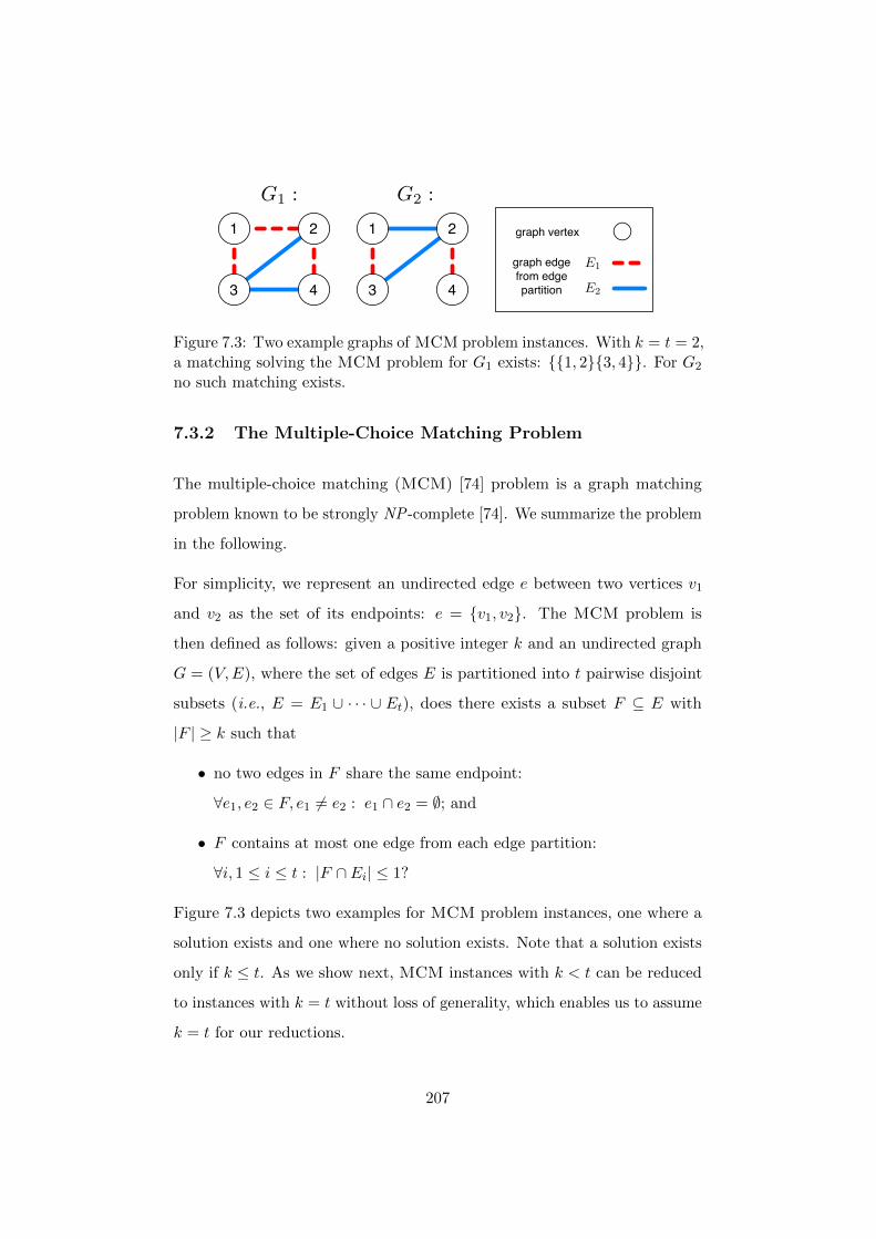
1
3
2
4
1
3
2
4
G1 : G2 :
graph vertex
graph edge from edge partition
E1
E2
Figure 7.3: Two example graphs of MCM problem instances. With k = t = 2,a matching solving the MCM problem for G1 exists: 1, 23, 4. For G2
no such matching exists.
7.3.2 The Multiple-Choice Matching Problem
The multiple-choice matching (MCM) [74] problem is a graph matching
problem known to be strongly NP -complete [74]. We summarize the problem
in the following.
For simplicity, we represent an undirected edge e between two vertices v1
and v2 as the set of its endpoints: e = v1, v2. The MCM problem is
then defined as follows: given a positive integer k and an undirected graph
G = (V,E), where the set of edges E is partitioned into t pairwise disjoint
subsets (i.e., E = E1 ∪ · · · ∪ Et), does there exists a subset F ⊆ E with
|F | ≥ k such that
• no two edges in F share the same endpoint:
∀e1, e2 ∈ F, e1 6= e2 : e1 ∩ e2 = ∅; and
• F contains at most one edge from each edge partition:
∀i, 1 ≤ i ≤ t : |F ∩ Ei| ≤ 1?
Figure 7.3 depicts two examples for MCM problem instances, one where a
solution exists and one where no solution exists. Note that a solution exists
only if k ≤ t. As we show next, MCM instances with k < t can be reduced
to instances with k = t without loss of generality, which enables us to assume
k = t for our reductions.
207
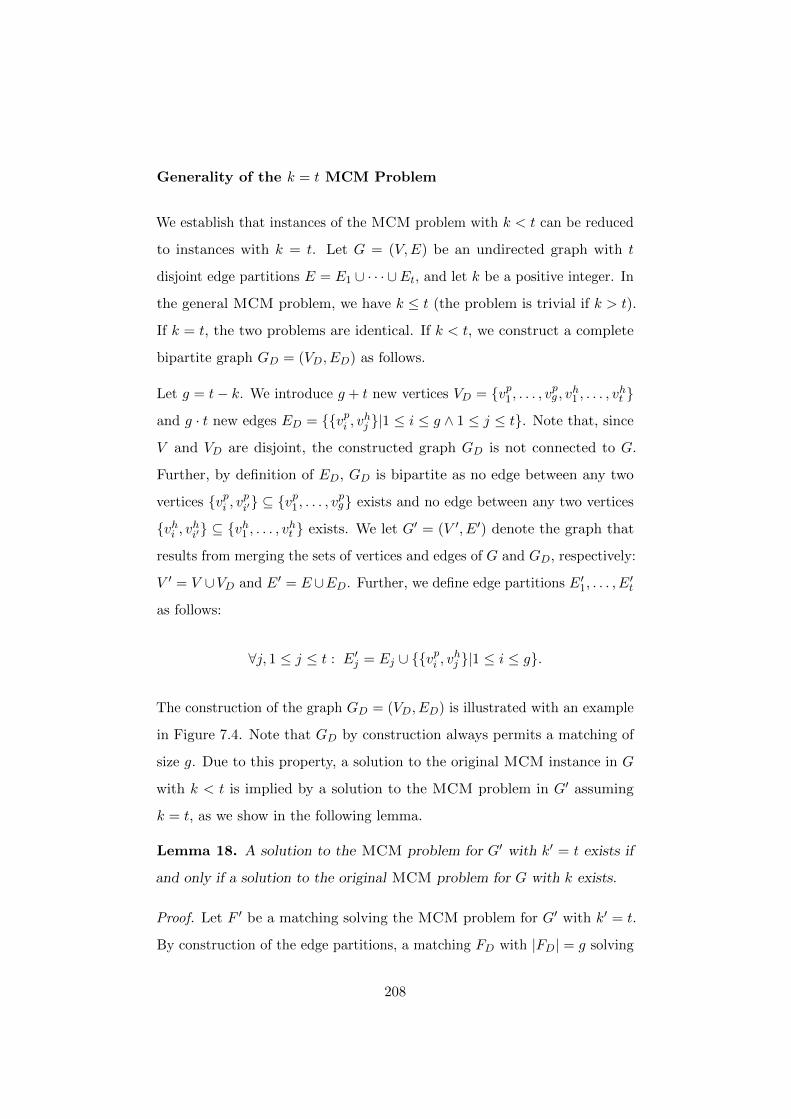
Generality of the k = t MCM Problem
We establish that instances of the MCM problem with k < t can be reduced
to instances with k = t. Let G = (V,E) be an undirected graph with t
disjoint edge partitions E = E1 ∪ · · · ∪Et, and let k be a positive integer. In
the general MCM problem, we have k ≤ t (the problem is trivial if k > t).
If k = t, the two problems are identical. If k < t, we construct a complete
bipartite graph GD = (VD, ED) as follows.
Let g = t− k. We introduce g + t new vertices VD = vp1 , . . . , vpg , vh1 , . . . , v
ht
and g · t new edges ED = vpi , vhj |1 ≤ i ≤ g ∧ 1 ≤ j ≤ t. Note that, since
V and VD are disjoint, the constructed graph GD is not connected to G.
Further, by definition of ED, GD is bipartite as no edge between any two
vertices vpi , vpi′ ⊆ v
p1 , . . . , v
pg exists and no edge between any two vertices
vhi , vhi′ ⊆ vh1 , . . . , vht exists. We let G′ = (V ′, E′) denote the graph that
results from merging the sets of vertices and edges of G and GD, respectively:
V ′ = V ∪VD and E′ = E∪ED. Further, we define edge partitions E′1, . . . , E′t
as follows:
∀j, 1 ≤ j ≤ t : E′j = Ej ∪ vpi , vhj |1 ≤ i ≤ g.
The construction of the graph GD = (VD, ED) is illustrated with an example
in Figure 7.4. Note that GD by construction always permits a matching of
size g. Due to this property, a solution to the original MCM instance in G
with k < t is implied by a solution to the MCM problem in G′ assuming
k = t, as we show in the following lemma.
Lemma 18. A solution to the MCM problem for G′ with k′ = t exists if
and only if a solution to the original MCM problem for G with k exists.
Proof. Let F ′ be a matching solving the MCM problem for G′ with k′ = t.
By construction of the edge partitions, a matching FD with |FD| = g solving
208
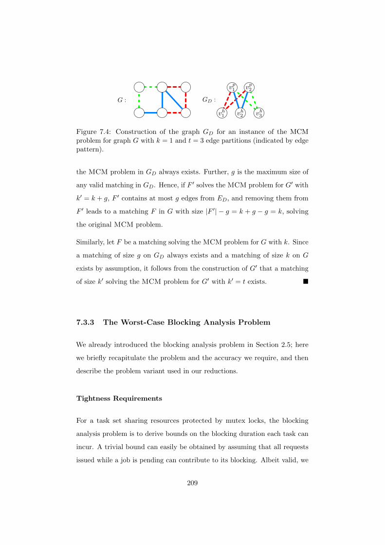
vp1 vp
2
vh2vh
1 vh3
G : GD :
Figure 7.4: Construction of the graph GD for an instance of the MCMproblem for graph G with k = 1 and t = 3 edge partitions (indicated by edgepattern).
the MCM problem in GD always exists. Further, g is the maximum size of
any valid matching in GD. Hence, if F ′ solves the MCM problem for G′ with
k′ = k + g, F ′ contains at most g edges from ED, and removing them from
F ′ leads to a matching F in G with size |F ′| − g = k + g − g = k, solving
the original MCM problem.
Similarly, let F be a matching solving the MCM problem for G with k. Since
a matching of size g on GD always exists and a matching of size k on G
exists by assumption, it follows from the construction of G′ that a matching
of size k′ solving the MCM problem for G′ with k′ = t exists.
7.3.3 The Worst-Case Blocking Analysis Problem
We already introduced the blocking analysis problem in Section 2.5; here
we briefly recapitulate the problem and the accuracy we require, and then
describe the problem variant used in our reductions.
Tightness Requirements
For a task set sharing resources protected by mutex locks, the blocking
analysis problem is to derive bounds on the blocking duration each task can
incur. A trivial bound can easily be obtained by assuming that all requests
issued while a job is pending can contribute to its blocking. Albeit valid, we
209
require the blocking analysis to yield tighter and less pessimistic bounds. In
particular, we require that:
• There exists no job arrival sequence and resulting schedule in which
more blocking than determined by the analysis is incurred. (The bound
is safe.)
• There exists a job arrival sequence and resulting schedule in which the
blocking duration determined by the analysis is incurred. (The bound
is tight.)
Note that we did not claim tightness of the blocking analysis for non-nested
spin locks presented in Section 6.3. However, under the job model considered
here (Section 7.3.1) and one job per processor, the analysis for non-nested
spin locks4 presented in Section 6.3 (assuming non-nested requests) yields
tight worst-case blocking bounds (i.e., true worst-case blocking durations):
for each blocking bound resulting from the analysis, a schedule can be
constructed under which this blocking is actually incurred.
We sketch the construction of such a schedule for F|* locks (F|N and F|P
locks behave similar in this setting since no preemptions can occur). Consider
the jobs Ji, J1, . . . , Jn−1, each assigned to its own processor, and let the result
of the blocking analysis presented in Section 6.3 be given in the form of
the assignment to blocking variables. First, observe that there is no arrival
blocking since each task is assigned to its own processor, and hence, the
blocking variables for arrival blocking are set to zero. Let Ji denote the task
under analysis. On a high level, we construct the schedule by letting Ji issue
each request simultaneously with one request for the same resource from
each other job that issues a blocking request according to the analysis result.
To that end, we first derive the number of blocking request for each job and
4The analysis for non-nested spin locks was presented for sporadic task sets and notfinite job sets, but can be trivially adapted.
210
resource: for a job Jx, let N ′x,q denote the number requests for `q issued by
Jx that block Ji in the schedule to be constructed:
∀`q ∈ Q : ∀x, 1 ≤ x ≤ n− 1 : N ′x,q ,Nx,q∑v=1
XSx,q,v.
We then construct the schedule as follows. All jobs are released at time
t = 0. For each request Ri,q,v for `q issued by Ji, select one request for `q
from each other job Jx with N ′x,q > 0 and denote this set of requests as R.
At time t, Ji’s request Ri,q,v and the requests in R are issued simultaneously,
and Ji’s request is blocked by all of the other requests. Decrement N ′x,q by
one for each other job, increment the time t by the cumulative maximum
critical section lengths of the requests Ri,q,v and R, and proceed with Ji’s
next request (if any). Once all of Ji’s requests have been considered, all jobs
complete, which concludes the construction of the schedule. By Constraints 8
and 23 in the analysis for F|N and F|P locks (Sections 6.3.2 and 6.3.6), the
number of blocking requests N ′x,q issued by job Jx for `q does not exceed
the number of Ji’s requests for `q. Hence, in the constructed schedule, Ji
incurs blocking for the same duration as determined by the analysis, and the
blocking analysis presented in Chapter 6 is tight in the setting we consider
for our reductions.
Note that the computationally inexpensive blocking analysis presented in
Chapter 6 does not generally yield tight blocking bounds. However, with the
simplified system model we assume here and without nesting, tightness can
be ensured. With nesting (and strong ordering guarantees), in contrast, the
blocking analysis problem is inherently hard with the same simplified system
model.
211

Optimization and Decision Variants
Given a set of jobs, a job under analysis, Ji, their resource accesses and a
mapping of jobs to processors, we denote the problem of deriving worst-case
blocking durations (i.e., tight bounds) as the blocking analysis optimization
problem BO, and the outcome of the blocking analysis for a job Ji is denoted
as Bi = BO(Ji).
BO: Blocking Analysis Optimization Problem
Input job set J1, . . . , Jn, job under analysis Ji, resource accesses,
partitioning.
Output Ji’s worst-case blocking duration BO(Ji).
In the problem definition above and in the following we assume that the re-
source accesses are encoded as a list of tuples (Ni,q, Li,q) giving the maximum
number of accesses of each job Ji with 1 ≤ i ≤ n to each resource q with
q ∈ Q and its maximum critical section length (analogous to the definition
of Ni,q and Li,q for tasks provided in Section 2.1.4). In addition, we assume
that the nesting relation between requests is encoded as a list containing
a tuple (Rx,q,s, Rx,q′,s′) if and only if Jx’s request Rx,q′,s′ is directly nested
within a different request Rx,q,s (i.e., Rx,q,s . Rx,q′,s′).
For our reductions, we also consider a decision variant of the blocking analysis
problem defined as follows: given a set of jobs, a job under analysis, Ji, and an
integral value Bi, the blocking analysis decision problem BD is the problem
of deciding if there exists a job arrival sequence and resulting schedule in
which Ji is blocked for at least Bi time units. We denote the outcome of the
decision problem (i.e., True or False) as BD(Ji, Bi).
212
BD: Blocking Analysis Decision Problem
Input job set J1, . . . , Jn, job under analysis Ji, resource accesses,
partitioning, Bi.
Output True if and only if BO(Ji) ≥ Bi.
The blocking analysis decision problem can be trivially reduced to the
optimization variant: given the solution to the optimization problem BO(Ji),
solutions to the decision problem BD(Ji, Bi) can be obtained by returning
True if and only if BO(Ji) ≥ Bi. The optimization variant can be reduced
(under Turing reductions, see Section 2.6.1) to the decision variant within
polynomial time, as we show next.
Given an oracle for the blocking analysis decision problem BD(Ji, Bi), the
solution to the optimization problem can be obtained by finding the maximal
integral value of B′i for which BD(Ji, Bi) evaluates to True. This can be
achieved by repeatedly evaluating BD(Ji, Bi) within a binary search over
the interval [0, Bmaxi ], where Bmax
i is a trivial upper bound on the blocking
that Ji can incur (e.g., the sum of all critical section lengths). Note that
Bmaxi grows exponentially with respect to the size of the problem instance
c: Bmaxi = O(2c). Here, c denotes the size of the binary representation of
the problem instance. Since the binary search terminates after O(log2Bmaxi )
steps, computing the solution to the optimization problem takes overall
O(log2Bmaxi ) = O(log2 2c) = O(c) steps with respect to the size of the
problem instance c.
For brevity, we denote the blocking analysis decision problems for FIFO-
ordered and priority-ordered locks as BDF and BDP , respectively. Further,
we denote the blocking that a job Jx incurs in a particular schedule S
(resulting from a particular job arrival sequence) as Bx(S).
In the following two sections, we show that the blocking analysis problem for
FIFO- and priority-ordered mutex locks is strongly NP -hard when nesting
213

of requests is allowed, even under the weak assumptions we stated in Sec-
tion 7.3.1. To that end, we present many-one reductions (see Section 2.6.1
for a brief summary) from the MCM problem to BDF and BDP problems,
respectively. That is, given an MCM problem, we construct a set of jobs
issuing nested requests such that the worst-case blocking duration Bi encodes
the answer to the MCM problem. We begin by reducing instances of the
MCM problem to the BDF problem.
7.4 Reduction of MCM to BDF
Before detailing the construction of the BDF instance from an MCM instance,
we first illustrate the high-level approach with an example.
7.4.1 An Example BDF Instance
Consider the graph G1 in Figure 7.3. The corresponding BDF instance is
shown in Figure 7.5a.
We model vertices as shared resources and edges as nested requests. More
specifically, edges are encoded as a request to a “dummy resource” `D that
contains two nested requests to the resources representing the endpoints of
the edge.
The two edge partitions in G1 (shown as dashed or solid edges in Figure 7.3)
correspond to processors P1 and P2 on which two jobs J1 and J2 issue the
requests that model the edges in G1.
The job J3 on processor P3 serves as a “probe”: by solving the BDF problem
for J3, which accesses only the dummy resource `D, we can infer whether G1
admits an MCM of size two. Finally, the job J4 on processor P4 serves to
transitively block J3 by creating contention for all resources corresponding
214

P1 P2 P3 P4
J1 J2 J3 J4
`2`1
`3
`4
`D
`D
`D
`D
`1
`2
`2 `3
`3 `4
`3
`D
`D
`2
`1
`4
`3
`2
`1
`4
shortlong
requests
processor
issuedrequests
assignedjob
(a) BDF problem constructed from G1 and k = t = 2.
`D
P1 P2 P3 P4
J1 J2 J3 J4
`2`1`3
`4
`1
`2 `2 `3
`3
`2
`1
`4
`3
`2
`1
`4
shortlong
requests
`D`D`D
`D
processor
issuedrequests
assignedjob
(b) BDF problem constructed from G2 and k = t = 2.
Figure 7.5: BDF problems constructed from G1 and G2.
to vertices in G1, as explained in more detail below.
7.4.2 Construction of the BDF Instance
Formally, given an MCM instance that consists of a graph G = (V,E), t
disjoint edge partitions E1, . . . , Et such that E1 ∪ · · · ∪ Et = E, and k = t
(without loss of generality, see Section 7.3.2), we construct a BDF instance
215

as follows.
For each vertex v ∈ V , there is one shared resource `v. In addition, there is
a single dummy resource `D. We consider t+ 2 processors, P1, . . . , Pt+2, and
t+ 2 jobs, J1, . . . , Jt+2, where each job Jj with 1 ≤ j ≤ t+ 2, is assigned to
processor Pj .
We construct requests with two basic critical section lengths: there are short
and long critical sections, with the corresponding lengths of ∆S , 1 and
∆L , 2 · |V |, respectively.
The jobs J1, . . . , Jt issue requests for the dummy resource `D with nested
requests to model edges, Jt+1 issues a single request for `D, and Jt+2 issues
a short request (of length ∆S) and a long request (of length ∆L) for each
resource `v corresponding to a vertex v ∈ V . More formally, the jobs issue
requests as follows.
• Jobs J1, . . . , Jt: For each edge ei = v, v′ in the edge partition Ej , job
Jj issues three requests: one request Rj,D,i for `D, one request Rj,v,i
for `v, and one request Rj,v′,i for `v′ . The critical section lengths are
Lj,D = 2 ·∆L, Lj,v = ∆L, and Lj,v′ = ∆L, respectively. The requests
are nested such that Rj,D,i . Rj,v,i, Rj,v′,i.
• Job Jt+1 issues one non-nested request Rt+1,D,1 for `D with critical
section length Lt+1,D = 1.
• Job Jt+2 issues for each resource `v with v ∈ V two non-nested requests:
Rt+2,v,1 and Rt+2,v,2. The critical section lengths are Lt+2,v,1 = ∆L
and Lt+2,v,2 = ∆S , respectively.
As the number of constructed jobs is linear in t ≤ |E| and the number of
constructed requests is linear in |V |, the reduction of the MCM instance to
an BDF instance requires only polynomial time with respect to the size of
the input graph.
216
7.4.3 Basic Idea: Jt+1’s Maximum Blocking Implies MCM
Answer
Recall that for a solution to the MCM problem to exist, there must be k
matched edges, and each vertex in the graph must be adjacent to at most one
matched edge. As we illustrate next with an example, this is equivalent to
requiring that, in a schedule S in which Jt+1 incurs the maximum blocking
possible (i.e., Bt+1(S) = Bt+1), Jt+1 is transitively blocked in S by Jt+2 with
exactly 2k of its long critical sections and none of its short critical sections.
Whether this is in fact the case can be inferred from Bt+1 due to the specific
values chosen for ∆S and ∆L.
Returning to the example BDF instance shown in Figure 7.5a, note how
the vertices v1, . . . , v4 in G1 correspond to the shared resources `1, . . . , `4 in
Figure 7.5a, and how edges in G1 map to nested requests issued by J1 and
J2. For instance, the dashed edge 1, 2 in G1 is represented as a request
for `D issued by J1 (which corresponds to E1) that contains nested requests
for `1 and `2. Similarly, the remaining dashed edges 1, 3 and 2, 4 are
also represented by nested requests issued by J1. The solid edges 2, 3 and
3, 4 are represented by similar requests issued by J2 (which corresponds to
E2).
Crucially, all requests for the resources `1, . . . , `4 issued by J1 and J2 are
nested within a request for `D. This ensures that (i) J3 can be transitively
delayed by J4’s requests and that (ii) J1 and J2’s requests for `1, . . . , `4 cannot
block each other since `D must be held in order to issue these requests.
Consider the worst case for J3, which is also illustrated in Figure 7.6a: J3’s
request for `D is delayed by one (outer) request for `D from both J1 and J2
each, and the nested requests issued by J1 and J2 are in turn blocked by
requests issued by J4, which transitively delays J3. Importantly, the total
217
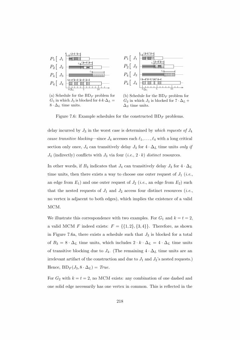
50 10
`1`D`2
`D`3 `4
`D
`1 `2 `3 `4
L
J1
J2
J3
J4
P4
P1
P2
P4
(a) Schedule for the BDF problem forG1 in which J3 is blocked for 4·k·∆L =8 ·∆L time units.
50 10
`1`D`2
`D
`D
`1 `2
`1 `3
`1 `3
L
J1
J2
J3
J4
P4
P1
P2
P4
(b) Schedule for the BDF problem forG2 in which J3 is blocked for 7 ·∆L +∆S time units.
Figure 7.6: Example schedules for the constructed BDF problems.
delay incurred by J3 in the worst case is determined by which requests of J4
cause transitive blocking—since J4 accesses each `1, . . . , `4 with a long critical
section only once, J4 can transitively delay J3 for 4 ·∆L time units only if
J4 (indirectly) conflicts with J3 via four (i.e., 2 · k) distinct resources.
In other words, if B3 indicates that J4 can transitively delay J3 for 4 ·∆L
time units, then there exists a way to choose one outer request of J1 (i.e.,
an edge from E1) and one outer request of J2 (i.e., an edge from E2) such
that the nested requests of J1 and J2 access four distinct resources (i.e.,
no vertex is adjacent to both edges), which implies the existence of a valid
MCM.
We illustrate this correspondence with two examples. For G1 and k = t = 2,
a valid MCM F indeed exists: F = 1, 2, 3, 4. Therefore, as shown
in Figure 7.6a, there exists a schedule such that J3 is blocked for a total
of B3 = 8 · ∆L time units, which includes 2 · k · ∆L = 4 · ∆L time units
of transitive blocking due to J4. (The remaining 4 ·∆L time units are an
irrelevant artifact of the construction and due to J1 and J2’s nested requests.)
Hence, BDF (J3, 8 ·∆L) = True.
For G2 with k = t = 2, no MCM exists: any combination of one dashed and
one solid edge necessarily has one vertex in common. This is reflected in the
218
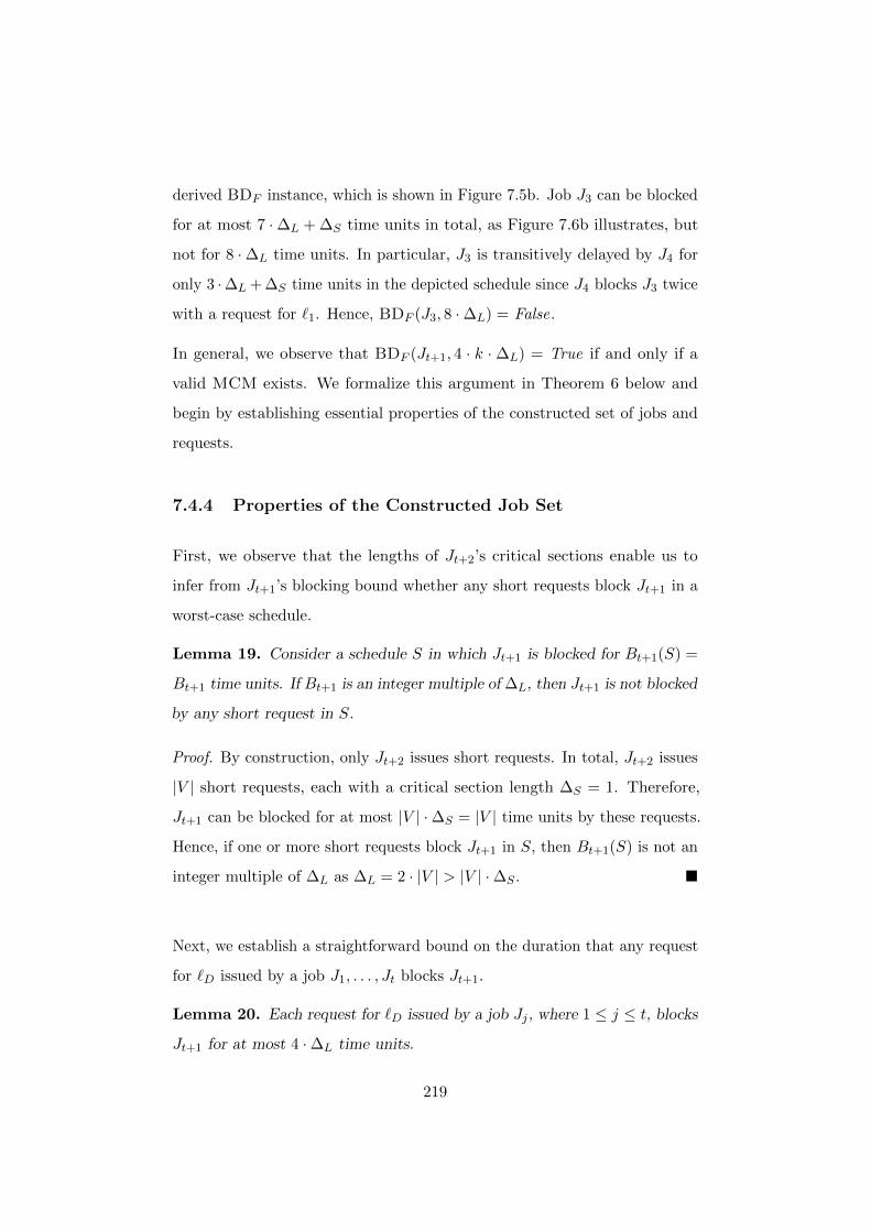
derived BDF instance, which is shown in Figure 7.5b. Job J3 can be blocked
for at most 7 ·∆L + ∆S time units in total, as Figure 7.6b illustrates, but
not for 8 ·∆L time units. In particular, J3 is transitively delayed by J4 for
only 3 ·∆L + ∆S time units in the depicted schedule since J4 blocks J3 twice
with a request for `1. Hence, BDF (J3, 8 ·∆L) = False.
In general, we observe that BDF (Jt+1, 4 · k ·∆L) = True if and only if a
valid MCM exists. We formalize this argument in Theorem 6 below and
begin by establishing essential properties of the constructed set of jobs and
requests.
7.4.4 Properties of the Constructed Job Set
First, we observe that the lengths of Jt+2’s critical sections enable us to
infer from Jt+1’s blocking bound whether any short requests block Jt+1 in a
worst-case schedule.
Lemma 19. Consider a schedule S in which Jt+1 is blocked for Bt+1(S) =
Bt+1 time units. If Bt+1 is an integer multiple of ∆L, then Jt+1 is not blocked
by any short request in S.
Proof. By construction, only Jt+2 issues short requests. In total, Jt+2 issues
|V | short requests, each with a critical section length ∆S = 1. Therefore,
Jt+1 can be blocked for at most |V | ·∆S = |V | time units by these requests.
Hence, if one or more short requests block Jt+1 in S, then Bt+1(S) is not an
integer multiple of ∆L as ∆L = 2 · |V | > |V | ·∆S .
Next, we establish a straightforward bound on the duration that any request
for `D issued by a job J1, . . . , Jt blocks Jt+1.
Lemma 20. Each request for `D issued by a job Jj , where 1 ≤ j ≤ t, blocks
Jt+1 for at most 4 ·∆L time units.
219

Proof. By construction, each request for `D from such a job Jj has a length
of 2 ·∆L time units and contains two nested requests for two resources `v1
and `v2 , where v1, v2 ∈ E. Also by construction, while Jj holds `D, it
can encounter contention only from Jt+2 (since all requests issued by jobs
J1, . . . , Jt are serialized by `D). In the worst case, each of Jj ’s nested requests
is hence blocked only by Jt+2’s matching long request of length ∆L. Jj thus
releases `D after at most 4 ·∆L time units.
From Lemma 20, we obtain an immediate upper bound on the total blocking
incurred by Jt+1 in any schedule.
Lemma 21. Bt+1 ≤ 4 · k ·∆L.
Proof. By construction, Jt+1 issues only a single request for `D. By Lemma 1,
Jt+1 is blocked by at most one request for `D from each job Jj with 1 ≤ j ≤ t.
(Jt+2 does not access `D.) By Lemma 20, each of these t = k requests blocks
Jt+1 for at most 4 ·∆L time units. Hence, Bt+1 ≤ 4 · k ·∆L.
Figure 7.6a illustrates Lemma 21 for the BDF instance constructed for G1.
In the depicted schedule, J3 is blocked in total for 4 · k ·∆L = 8 ·∆L time
units, and no other request can further block J3. Note that none of the
resources `1, . . . , `4 is requested more than once within a request for `D from
J1 or J2 that blocks J3. In fact, as we show with the next lemma, this is
generally the case if the job J3 is blocked for 4 · k ·∆L time units.
Lemma 22. Let S denote a schedule of the constructed job set. If Bt+1(S) =
4 · k ·∆L, then each resource `v with v ∈ V is requested within at most one
request for `D that blocks Jt+1.
Proof. From Lemma 21, it follows that S is a worst-case schedule for Jt+1.
Hence, if a job Jj with 1 ≤ j ≤ t blocks Jt+1 with a request for `D, then
220

each nested request therein encounters contention from Jt+2. (Otherwise,
S would not be a worst-case schedule.) By Lemma 19, since Bt+1(S) is an
integer multiple of ∆L, Jt+1 is (transitively) blocked only by long requests
in S. Since Jt+2 issues only a single long request for each `v (with v ∈ V ),
this implies that each resource `v with v ∈ V is requested within at most
one request for `D that blocks Jt+1.
With Lemma 22 it can be shown that, if BDF (Jt+1, 4 · k · ∆L) = True,
then there is a matching such that no vertex is adjacent to more than one
matched edge. To solve the MCM problem, we additionally have to show
that such a matching contains exactly one edge from each edge partition.
To this end, we next show that, if Bt+1(S) = 4 · k ·∆L, then exactly one
request for `D (corresponding to an edge) from each of the jobs J1, . . . , Jt
(each corresponding to an edge partition) blocks Jt+1.
Lemma 23. Let S denote a schedule of the constructed job set. If Bt+1(S) =
4 · k ·∆L, then each Jj with 1 ≤ j ≤ t blocks Jt+1 with exactly one request
for `D.
Proof. By Lemma 1, each of the t jobs J1, . . . , Jt can block Jt+1 in S with at
most one request for `D. (Jt+2 does not access `D.) Further, by Lemma 20,
a request for `D by a job Jj with 1 ≤ j ≤ t blocks Jt+1 for at most 4 ·∆L
time units. Hence, the number of such requests that block Jt+1 in S is at
least Bt+1(S)/(4 ·∆L) = k = t. Hence, each Jj with 1 ≤ j ≤ t blocks Jt+1
exactly once in S.
With these lemmas in place, we next show that solving the BDF problem
for the constructed instance is equivalent to solving the MCM problem for
the input instance.
221

Theorem 6. A matching F solving the MCM problem exists if and only if
BDF (Jt+1, 4 · k ·∆L) = True.
Proof. We show the following two implications to prove equivalence:
• =⇒: If BDF (Jt+1, 4 · k ·∆L) = True, then there exists a matching F
solving the MCM problem.
• ⇐=: If there exists a matching F solving the MCM problem, then
BDF (Jt+1, 4 · k ·∆L) = True.
=⇒: By the definition of BDF , it follows from BDF (Jt+1, 4 · k ·∆L) = True
that there exists a schedule S such that Bt+1(S) = 4 · k ·∆L. We construct
a matching F that solves the MCM problem from the requests for `D that
block Jt+1 in S.
For each job Jj with 1 ≤ j ≤ t, let Rj,D,s denote the request for `D issued
by Jj that blocks Jt+1 in S. For brevity, let edge(Rj,D,s) denote the edge
v1, v2 corresponding to Rj,D,s, and let F contain all edges represented by
requests for `D that block Jt+1: F ,⋃
1≤j≤tedge(Rj,D,s).
By Lemma 23, exactly one request for `D from each job J1, . . . , Jt blocks
Jt+1; F hence contains |F | = t edges in total and exactly one edge per
edge partition. Further, by Lemma 22, for each resource `v with v ∈ V at
most one request for `v is nested within a blocking request for `D from any
processor. Hence, each vertex v ∈ V is adjacent to at most one edge in F .
Therefore F is a matching solving the MCM problem.
⇐=: Let F be a matching solving the MCM problem for a graph G = (V,E),
edge partitions E1, . . . , Et, and k = t. Consider a schedule S in which Jt+1 is
maximally (i.e., for the full critical section length) blocked by each request for
`D that corresponds to an edge in F . Since F is an MCM in G, F contains
exactly one edge from each edge partition. Then, by construction, Jt+1 is
blocked by exactly one request for `D from each processor Pj , 1 ≤ j ≤ t.
222
As F is a matching, each vertex v ∈ V is adjacent to at most one edge in
F . Since vertices in the MCM instance correspond to resources in the BDF
instance, each resource `v with v ∈ V is requested within at most one request
for `D that blocks Jt+1 in S. Then each request for `v with v ∈ V nested
within a blocking request for `D can be blocked by the long request for `v
issued by Jt+2, and thus each blocking request for `D can block Jt+1 for
4 ·∆L time units. Since k = t requests for `D in total block Jt+1, there exists
a schedule S such that job Jt+1 is blocked for 4 · k ·∆L time units. Then
BDF (Jt+1, 4 · k ·∆L) = True.
As described in Section 7.4.2, the construction of the BDF instance requires
only polynomial time with respect to the MCM instance size. Since instances
of the MCM decision problem can be solved via reduction to BDF , and
since the MCM problem is strongly NP -complete, it follows that BDF is
strongly NP -hard.
Next, we show that the blocking analysis decision problem for priority-ordered
locks in the presence of nested critical sections on multiprocessors is strongly
NP -hard as well.
7.5 Reduction of MCM to BDP
The reduction to BDP follows in large parts the same structure as the one for
BDF , but must deal with the slightly weaker progress guarantees offered by
priority-ordered locks. With FIFO-ordered locks, each request can be blocked
at most once by a request from each other processor (Lemma 1). This fact
was exploited to ensure that exactly one edge in each edge partition of a given
MCM instance is contained in a matching. Priority-ordered locks, however,
do not have this ordering property, and hence the previous approach cannot
223
be used directly. To ensure that one edge per partition is matched, we instead
use multiple different dummy resources and an appropriate assignment of
request priorities. Next, we explain the approach in detail.
7.5.1 Main Differences to BDF Reduction
At a high level, the constructed BDP instance is similar to the BDF reduction,
with the following exceptions.
• We use one dummy resource `jD for each processor Pj with 1 ≤ j ≤ t
(instead of the single global `D in BDF ).
• The job Jt+1 issues a request for each dummy resource `jD (instead of
a single request for `D in BDF ).
• Each job Jj with 1 ≤ j ≤ t issues requests for the “local” dummy
resource `jD (instead of for the global `D in BDF ).
• An additional resource `U serializes requests of the jobs J1, . . . , Jt: each
job Jj ’s requests for the dummy resource `jD (with 1 ≤ j ≤ t) are nested
in a request for `U .
The basic idea of the reduction of MCM to BDP is the same as for the
reduction to BDF : the solution to the MCM problem can be inferred from
Jt+1’s blocking bound. We illustrate the reduction of MCM to BDP with
two examples. Figures 7.7a and 7.7b show the BDP instances constructed
for the graphs G1 and G2, respectively, as given in Figure 7.3. The priorities
of the requests are assigned as follows. We use three distinct priority levels:
high, medium, and low. J3’s requests are issued with high priority, J1’s and
J2’s requests are issued with medium priority, and J4’s requests are issued
with low priority.
Recall that for graph G1 and k = t = 2, a matching F solving the MCM
224
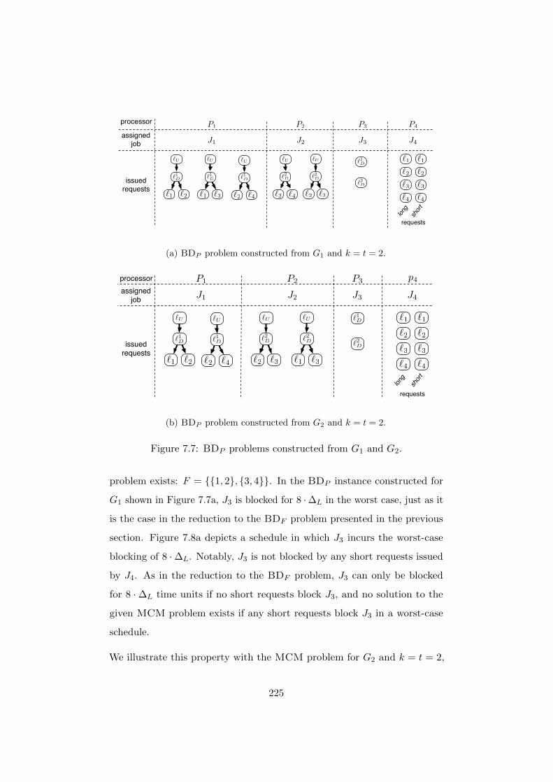
P1 P2 P3 P4
J1 J2 J3 J4
`2`1 `3 `4`1 `2 `2 `3`3
`2
`1
`4
`3
`2
`1
`4
shortlong
requests
`1D `2D
`U
`1D
`U `U `U
`1D `2D
`U
`3 `4
`1D
processor
assignedjob
issuedrequests
`2D
(a) BDP problem constructed from G1 and k = t = 2.
P1 P2 P3 p4
J1 J2 J3 J4
`2`1 `3`4 `1`2 `2 `3`3
`2
`1
`4
`3
`2
`1
`4
shortlongrequests
`1D `2D
`U
`1D
`U`U `U `1D
`2D
processor
issuedrequests
assignedjob
`2D
(b) BDP problem constructed from G2 and k = t = 2.
Figure 7.7: BDP problems constructed from G1 and G2.
problem exists: F = 1, 2, 3, 4. In the BDP instance constructed for
G1 shown in Figure 7.7a, J3 is blocked for 8 ·∆L in the worst case, just as it
is the case in the reduction to the BDF problem presented in the previous
section. Figure 7.8a depicts a schedule in which J3 incurs the worst-case
blocking of 8 ·∆L. Notably, J3 is not blocked by any short requests issued
by J4. As in the reduction to the BDF problem, J3 can only be blocked
for 8 ·∆L time units if no short requests block J3, and no solution to the
given MCM problem exists if any short requests block J3 in a worst-case
schedule.
We illustrate this property with the MCM problem for G2 and k = t = 2,
225
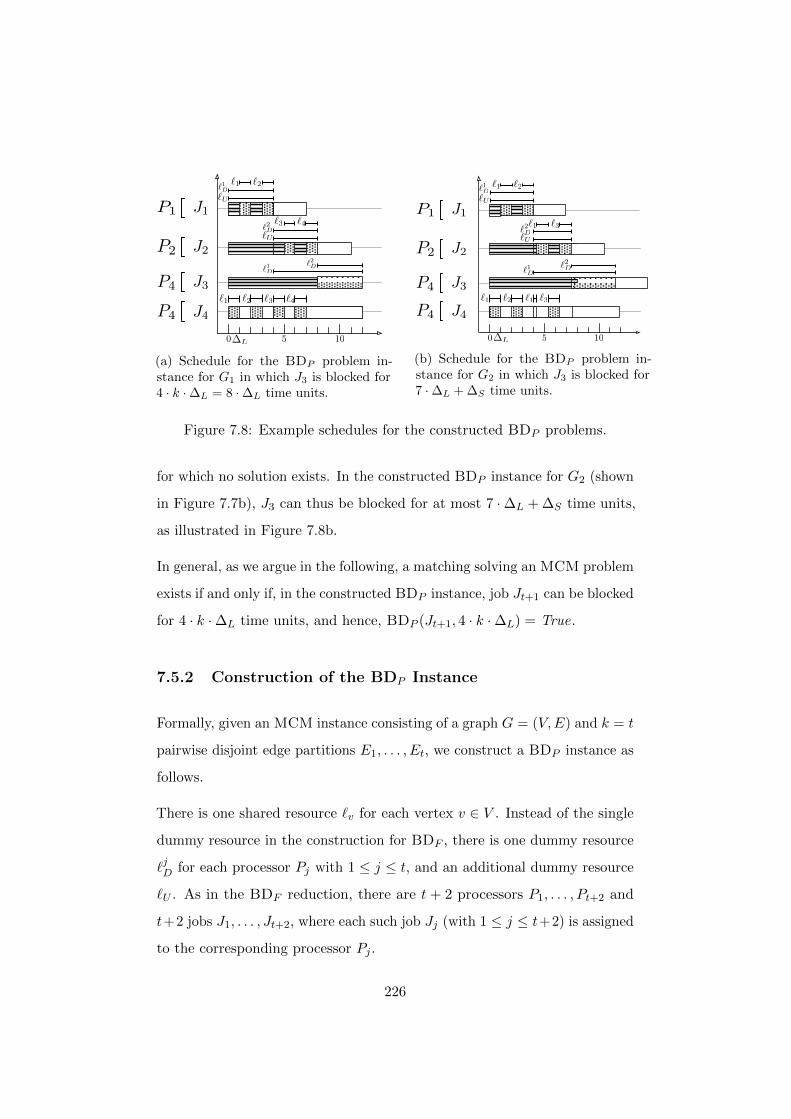
50 10
`1 `2
`3 `4
`1D
`1D
`2D
`U
`2D
`U
`1 `2 `3 `4
L
J1
J2
J3
J4
P4
P1
P2
P4
(a) Schedule for the BDP problem in-stance for G1 in which J3 is blocked for4 · k ·∆L = 8 ·∆L time units.
50 10
J1
J2
J3
J4
`1 `2
`1 `2 `3
`1D
`2D
`U
`1
`1 `3`U
`1D`2D
L
P4
P1
P2
P4
(b) Schedule for the BDP problem in-stance for G2 in which J3 is blocked for7 ·∆L + ∆S time units.
Figure 7.8: Example schedules for the constructed BDP problems.
for which no solution exists. In the constructed BDP instance for G2 (shown
in Figure 7.7b), J3 can thus be blocked for at most 7 ·∆L + ∆S time units,
as illustrated in Figure 7.8b.
In general, as we argue in the following, a matching solving an MCM problem
exists if and only if, in the constructed BDP instance, job Jt+1 can be blocked
for 4 · k ·∆L time units, and hence, BDP (Jt+1, 4 · k ·∆L) = True.
7.5.2 Construction of the BDP Instance
Formally, given an MCM instance consisting of a graph G = (V,E) and k = t
pairwise disjoint edge partitions E1, . . . , Et, we construct a BDP instance as
follows.
There is one shared resource `v for each vertex v ∈ V . Instead of the single
dummy resource in the construction for BDF , there is one dummy resource
`jD for each processor Pj with 1 ≤ j ≤ t, and an additional dummy resource
`U . As in the BDF reduction, there are t + 2 processors P1, . . . , Pt+2 and
t+2 jobs J1, . . . , Jt+2, where each such job Jj (with 1 ≤ j ≤ t+2) is assigned
to the corresponding processor Pj .
226
As in the BDF reduction, the critical sections of these jobs are either short
(i.e., of length ∆S , 1) or long (i.e., of length ∆L , 2 · |V |), and graph
edges are modeled as nested requests. In contrast to the reduction to BDF ,
where all of these requests were nested within a request for the single dummy
resource `D, the requests modeling an edge from edge partition Ej are nested
within a request for the dummy resource `jD. Further, each request for `jD
issued by a job Jj with 1 ≤ j ≤ t is nested within a request for `U . The jobs
issue requests as follows.
• Jobs J1, . . . , Jt: For each edge ei = v, v′ in the edge partition Ej ,
the job Jj issues four requests: one request Rj,U,i for `U , one request
Rj,Dj ,i for `jD, one request Rj,v,i for `v, and one request Rj,v′,i for `v′ ,
where Rj,U,i .Rj,Dj ,i .Rj,v,i, Rj,v′,i, and Lj,U = 2 ·∆L, Lj,Dj = 2 ·∆L,
Lj,v = ∆L, and Lj,v′ = ∆L.
• Job Jt+1 issues one non-nested request Rt+1,Dj ,1 for each dummy
resource `jD (where 1 ≤ j ≤ t) with Lt+1,Dj = 1.
• Job Jt+2 issues for each resource `v (where v ∈ V ) two non-nested
requests Rt+2,v,1 and Rt+2,v,2, where Lt+2,v,1 = ∆L and Lt+2,v,2 = ∆S .
Since we use priority-ordered locks in the construction of the BDP instance,
a priority has to be assigned to each request. We use three priority levels:
high, medium, and low. The requests issued by job Jt+1 all have high priority,
while the requests issued by J1, . . . , Jt all have medium priority (which is
strictly lower than high priority). The requests issued by Jt+2 all have low
priority (which is strictly lower than medium priority).
As with the BDF reduction, reducing an MCM instance to the BDP problem
requires only polynomial time with respect the input size as the number of
constructed jobs is linear in t ≤ |E| and the number of constructed requests
is linear in |V |.
227

7.5.3 Properties of the Constructed Job Set
The choice of critical section length of the requests issued by Jt+2 allows us
to infer from Jt+1’s blocking bound whether Jt+1 is blocked by any short
requests in a worst-case schedule.
Lemma 24. Consider a schedule S in which Jt+1 is blocked for Bt+1(S) =
Bt+1 time units. If Bt+1 is an integer multiple of ∆L, then Jt+1 is not blocked
by any short request in S.
Proof. Analogous to the proof of Lemma 19. By construction, there exist
only |V | short requests (issued by Jt+2), each of length ∆S = 1. Since
∆L = 2 · |V | > |V | ·∆S , if any of the short requests block Jt+1 in S, then
Bt+1(S)/∆L is not integer.
In the next lemma, we state a bound on the blocking duration that Jt+1 can in-
cur due to any single request for `D issued by one of the jobs J1, . . . , Jt.
Lemma 25. Each request for `jD issued by a job Jj , where 1 ≤ j ≤ t, blocks
Jt+1 for at most 4 ·∆L time units.
Proof. Analogous to the proof of Lemma 20. By construction, each request
for `jD from such a job Jj has a length of 2 ·∆L time units and contains two
nested requests for two resources `v1 and `v2 , where v1, v2 ∈ E. Also by
construction, while Jj holds `jD, it can encounter contention only from Jt+2
(since all requests issued by jobs J1, . . . , Jt are serialized by `U ). In the worst
case, each of Jj ’s nested requests is hence blocked only by Jt+2’s matching
long request of length ∆L. Jj thus releases `jD after at most 4 ·∆L time units.
Lemma 25 leads to a straightforward upper bound on the total blocking
228
incurred by Jt+1 in any schedule.
Lemma 26. Bt+1 ≤ 4 · k ·∆L.
Proof. Analogous to the proof of Lemma 21. By construction, Jt+1 issues
only a single request for each resource `jD with 1 ≤ j ≤ t. Since Jt+1’s
requests have higher priority than the requests issued by the jobs J1, . . . , Jt,
each of the requests for `jD with 1 ≤ j ≤ t issued by Jt+1 can be blocked
by at most one request for `jD from Jj . By Lemma 25, each of these t = k
requests blocks Jt+1 for at most 4 ·∆L time units. Hence, Bt+1 ≤ 4 ·k ·∆L.
Lemma 26 is illustrated in Figure 7.8a for the BDP instance constructed
from G1. In this schedule, J3 is blocked for 4 · k ·∆L = 8 ·∆L time units in
total, and J3 cannot be further blocked by any other request. Just as it is
the case with the BDF reduction (recall Figure 7.6a), none of the resources
`1, . . . , `4 is requested more than once within the requests for `1D and `2D
issued by J1 and J2 that block J3. As stated next, this is generally the case
if J3 is blocked for 4 · k ·∆L time units.
Lemma 27. Let S denote a schedule of the constructed job set. If Bt+1(S) =
4 · k ·∆L, then each resource `v with v ∈ V is requested within at most one
request for any resource `jD with 1 ≤ j ≤ t that blocks Jt+1.
Proof. Analogous to the proof of Lemma 22. From Lemma 26, it follows that
S is a worst-case schedule for Jt+1, and thus if a job Jj with 1 ≤ j ≤ t blocks
Jt+1 with a request for `jD, then each nested request therein encounters
contention from Jt+2.
By Lemma 24, since Bt+1(S) is an integer multiple of ∆L, Jt+1 is blocked
only by long requests in S. Since Jt+2 issues only a single long request
for each `v (with v ∈ V ), this implies that each resource `v with v ∈ V is
requested within at most one request for any `jD with 1 ≤ j ≤ t that blocks
229
Jt+1.
If BDP (Jt+1, 4 ·k ·∆L) = True, then Lemma 27 allows inferring the existence
of a matching such that no two matched edges share a vertex, and that exactly
one edge from each edge partition is contained in the implied matching.
Lemma 28. Let S denote a schedule of the constructed job set. If Bt+1(S) =
4 · k ·∆L, then each Jj with 1 ≤ j ≤ t blocks Jt+1 with exactly one request
for `jD.
Proof. Analogous to the proof of Lemma 23. Since Jt+1’s requests have
higher priority than the requests of jobs J1, . . . , Jt, each of Jt+1’s requests for
a resource `jD with 1 ≤ j ≤ t can be blocked at most once by a request for `jD
issued by Jj . By Lemma 25, each request for `jD from Jj with 1 ≤ j ≤ t can
block Jt+1 for at most 4 ·∆L time units. Hence, Jt+1 is blocked by exactly
one request from each processor P1, . . . , Pt.
With the stated lemmas, it can be shown that solving the provided MCM
problem instance is equivalent to solving the constructed BDP instance.
Theorem 7. A matching F solving the MCM problem exists if and only if
BDP (Jt+1, 4 · k ·∆L) = True.
Proof. Analogous to the proof of Theorem 6. We show the following two
implications to prove equivalence:
• =⇒: If BDP (Jt+1, 4 · k ·∆L) = True, then there exists a matching F
solving the MCM problem.
• ⇐=: If there exists a matching F solving the MCM problem, then
BDP (Jt+1, 4 · k ·∆L) = True.
=⇒: It follows from BDP (Jt+1, 4 ·k ·∆L) = True that there exists a schedule
230
S such that Bt+1(S) = 4 ·k ·∆L. We construct an MCM F from the requests
that block Jt+1 in S.
For each job Jj with 1 ≤ j ≤ t, let Rj,Dj ,s denote the request for `jD
issued by Jj that blocks Jt+1 in S. Let edge(Rj,Dj ,s) denote the edge
v1, v2 corresponding to Rj,Dj ,s, and let F contain all edges represented
by requests for the resources `jD with 1 ≤ j ≤ t that block Jt+1: F ,⋃1≤j≤tedge(Rj,Dj ,s).
By Lemma 28, each job Jj with 1 ≤ j ≤ t blocks Jt+1 with exactly one
request for `jD; F hence contains |F | = t edges in total and exactly one edge
per edge partition. By Lemma 27, for each resource `v with v ∈ V at most
one request for `v is nested within a blocking request for any resource `jD
with 1 ≤ j ≤ t. Hence, each vertex v ∈ V is adjacent to at most one edge in
F . F is thus a matching solving the MCM problem.
⇐=: Let F be a matching solving the MCM problem for a graph G = (V,E),
edge partitions E1, . . . , Et and k = t. Consider a schedule S in which Jt+1 is
blocked by each request for `jD with 1 ≤ j ≤ t that corresponds to an edge
in F . Since F is an MCM in G, F contains exactly one edge from each
edge partition. Then, by construction, Jt+1 is blocked from each processor
Pj , 1 ≤ j ≤ t by exactly one request for `jD.
As F is a matching, each vertex v ∈ V is adjacent to at most one edge
in F . Since vertices in the MCM instance correspond to resources in the
BDP instance, each resource `v with v ∈ V is requested within at most one
request for any of the resources `1D, . . . , `tD that blocks Jt+1 in S. Then each
request for `v with v ∈ V nested within a blocking request for a resource
`jD with 1 ≤ j ≤ t can be blocked by the long request for `v issued by
Jt+2, and thus each blocking request for a resource `jD with 1 ≤ j ≤ t can
block Jt+1 for 4 · ∆L time units. Since k = t requests for the resources
`1D, . . . , `tD in total block Jt+1, there exists a schedule S such that job Jt+1
231
is blocked for 4 ·k ·∆L time units, and hence BDP (Jt+1, 4 ·k ·∆L) = True.
Since instances of the MCM problem with k = t can be solved by solving
the constructed BDP instance, and since the MCM problem is strongly
NP -complete, BDP is strongly NP -hard.
7.6 A Special Case: Blocking Analysis for Unordered
Nested Locks within Polynomial Time
In contrast to priority-ordered and FIFO-ordered locks, unordered locks
do not ensure any specific ordering of requests. As a consequence, each
request can be blocked by any remote request for the same resource, unless
both requests are issued within outer critical sections accessing the same
resource. Interestingly, this rules out reductions similar to those given in
Sections 7.4 and 7.5. To demonstrate this, we establish in this section that,
in a special case that matches the setup used to establish the hardness results
in the preceding two sections, the blocking analysis optimization problem for
unordered spin locks can be solved in polynomial time.
Our reductions in Sections 7.4 and 7.5 are oblivious to the scheduling policy
employed since at most one job is assigned to each processor. In this section,
we consider a similar setting for the analysis of unordered nested locks to
rule out any effects related to the scheduling policy. Specifically, we assume
that
• job release times are unknown (just as before),
• each job is assigned to its own dedicated processor,
• jobs can issue their requests at any point in their execution and in any
order, and
232
• no minimum nor maximum separation between the releases of any two
jobs or any two critical sections can be assumed.
Although the lack of knowledge about the order in which requests are
issued, a minimum or maximum separation between them, or their concrete
timing may appear to be a rather weak assumption, these assumptions were
commonly made in prior work on blocking analysis: neither the classic MSRP
analysis [72], the improved holistic one [43, Ch. 5], nor our spin lock analysis
framework presented in Chapter 6 assume or exploit such information, and
analyses for other lock types make similar assumptions (e.g., [36, 141]. Note
that the reductions given in Sections 7.4 and 7.5 match these assumptions,
that is, this restricted special case suffices to show strong NP -hardness of
the blocking analysis problem for FIFO- and priority-ordered locks in the
presence of nested critical sections.
In the following, we show that, with unordered locks, this special case can
be solved in polynomial time, which establishes that reductions similar to
those given in Sections 7.4 and 7.5 are inapplicable to this class of locks.5
Without loss of generality, we focus on computing the blocking bound for
job J1.
Our approach relies on constructing a “blocking graph” in which requests
are encoded as vertices, and the nesting relationship as well as the potential
blocking between two requests are encoded as edges. In the following, we
show how to construct the blocking graph such that the blocking optimization
problem reduces to a simple reachability check.
5To be clear, it does not establish a tractability result for the unrestricted general case,as the general case requires addressing further issues unrelated to locking per se (e.g.,precisely characterizing the possible interleavings of multiple jobs on each processor) thatwe chose to exclude here.
233
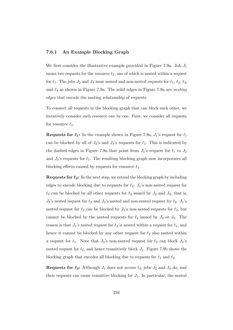
7.6.1 An Example Blocking Graph
We first consider the illustrative example provided in Figure 7.9a. Job J1
issues two requests for the resource `2, one of which is nested within a request
for `1. The jobs J2 and J3 issue nested and non-nested requests for `1, `2, `3,
and `4 as shown in Figure 7.9a. The solid edges in Figure 7.9a are nesting
edges that encode the nesting relationship of requests.
To connect all requests in the blocking graph that can block each other, we
iteratively consider each resource one by one. First, we consider all requests
for resource `1.
Requests for `1: In the example shown in Figure 7.9a, J1’s request for `1
can be blocked by all of J2’s and J3’s requests for `1. This is indicated by
the dashed edges in Figure 7.9a that point from J1’s request for `1 to J2
and J3’s requests for `1. The resulting blocking graph now incorporates all
blocking effects caused by requests for resource `1.
Requests for `2: In the next step, we extend the blocking graph by including
edges to encode blocking due to requests for `2. J1’s non-nested request for
`2 can be blocked by all other requests for `2 issued by J2 and J3, that is,
J2’s nested request for `2 and J3’s nested and non-nested request for `2. J1’s
nested request for `2 can be blocked by J3’s non-nested requests for `2, but
cannot be blocked by the nested requests for `2 issued by J2 or J3. The
reason is that J1’s nested request for `2 is nested within a request for `1, and
hence it cannot be blocked by any other request for `2 also nested within
a request for `1. Note that J3’s non-nested request for `2 can block J2’s
nested request for `2, and hence transitively block J1. Figure 7.9b shows the
blocking graph that encodes all blocking due to requests for `1 and `2.
Requests for `3: Although J1 does not access `3, jobs J2 and J3 do, and
their requests can cause transitive blocking for J1. In particular, the nested
234

p1 p2 p3
J1 J2 J3
`2 `2
`3
`2
`1 `1
`1
`3
`1
`4
`4
`2
`3
`4
`2
(a) Considered resources:`1.
`2 `2
`3
`2
`1 `1
`1
`3
`1
`2
`2
p1 p2 p3
J1 J2 J3
`4
`4
`3
`4
(b) Considered resources:`1 and `2.
`2 `2
`3
`2
`1 `1
`1
`3
`1
`2
`2
p1 p2 p3
J1 J2 J3
`4
`4
`3
`4
(c) Considered resources:`1, . . . , `4.
Figure 7.9: Construction of the blocking graph for jobs J1, . . . , J3. Dashedarrows indicate how J1 can be directly or transitively blocked by remoterequests.
request for `3 issued by J2 is nested within a request for `1 that can block
J1. This nested request for `3 can be blocked by J3’s request for `3, which
can then transitively block J1. In Figure 7.9c, this is illustrated with an
additional dashed arrow from J2’s nested request for `3 to J3’s request for
`3.
Note that J2’s non-nested request for `3 cannot block J1: it is not issued
within a request that already blocks J1, nor can it transitively delay a request
that blocks J1. In particular, if J3’s request for `3 blocks J1, then it does so
transitively by blocking J2’s request for `3 that is nested within a request for
`1 (which in turn blocks J1). In this case, however, J2’s non-nested request
for `3 is either already completed or not issued yet, as otherwise two of
J2’s outermost requests would be pending at the same time, which is not
possible.
Requests for `4: The requests for `4 cannot block J1 as they are not nested
within any request that can block J1, nor does J1 issue any requests for `4.
Hence, although the requests for `4 issued by J2 and J3 can block each other,
235
they cannot block J1.
We denote the resulting graph as blocking graph, since by construction it has
the property that a vertex is reachable from J1 if and only if the corresponding
request can block J1. We formalize this property in Lemmas 29 and 30.
7.6.2 Blocking Graph Construction
In the following, we let e = (v1, v2) denote a directed edge from vertex v1
to vertex v2. Recall that we require the existence of a partial order < such
that if a request Rx,q′,s′ issued by Jx is nested within a request Rx,q,s, then
q < q′. Let `1, . . . , `nr denote a sequence of shared resources that satisfies
the partial order on requests. That is, a request for `i cannot be nested in
any requests for `j with j > i.
The blocking graph is a directed, acyclic graph G = (V,E) that is constructed
as follows. The set of vertices V consists of one vertex for each request Rx,q,r
issued by any job Jx in the system: V = vx,q,r| ∃Rx,q,r.
As shown in Figure 7.9c, we construct G with two kinds of edges: nesting
edges En (shown as solid arrows) and interference edges Ei (shown as dashed
arrows). With nesting edges we model the nesting relation among requests
in G, and with interference edges we model direct or transitive blocking of
J1’s requests. The set of nesting edges is defined as follows:
En = (vx,p,w, vx,q,r)|Rx,p,w . Rx,q,r. (1)
We define the set of interference edges inductively by considering requests
for only one resource in each step, as we did in the example in Section 7.6.1.
That is, we define Eit with 1 ≤ t ≤ nr to be the set of all interference edges
among requests for the resources `1 up to `t. We start with the subset Ei1
236
of Ei that contains only edges to requests for `1. (Ei1 corresponds to the
dashed edges in Figure 7.9a.) Formally, an edge (Rx,1,v, Ry,1,w) is in Ei1 if
and only if Rx,1,v is a request for `1 issued by J1 and Ry,1,w is a remote
request (because J1 cannot block itself) for `1:
(v1,1,v, vy,1,w) ∈ Ei1 ⇐⇒ ∃R1,1,v ∧ ∃Ry,1,w ∧ y 6= 1.
Based on Ei1, we define G1 = (V,E1) to be the blocking graph with the edges
E1 = Ei1 ∪ En, similar to Figure 7.9a. Recall that nr denotes the number
of shared resources. Similar to the inductive definition of Eit , we define the
respective blocking graph Gt with 1 ≤ t ≤ nr accordingly: Gt = (V,En∪Eit).
Intuitively, the (partial) blocking graph Gt considers all requests for the
resources `1, . . . , `t and the resulting potential blocking.
Before we show how the set Eit+1 can be constructed from Eit , we introduce
the following notation and definitions.
• The predicate reachable(G, Jx, vx,q,r) holds if and only if a path in G
from a request issued by Jx to the request Rx,q,r exists. All requests of
Jx are defined to be reachable.
• The set of resources that job Jx must hold when it issues the request
Rx,q,v is given by held(Rx,q,v). For instance, in the example illustrated
in Figure 7.9, job J2 must already hold a lock on the resource `1 when
it requests `2,
• Given a partial blocking graph G′ and a set of requests W , G′ \W
denotes the graph that results from removing (from G′) all vertices
corresponding to requests in W or (transitively) nested within requests
in W .
237

• The conflict set of a request Ry,t,s is given by
conf (Ry,t,s) = Rz,u,v | `u ∈ held(Ry,t,s) ∨ z = y,
that is, the conflict set contains requests that either are also issued by
the same job or that pertain that to a resource that Jy must already
hold to issue Ry,t,s.
Based on the notion of the conflict set, we define the set of non-conflicting
edges Ei,NCt for a resource `t with 2 ≤ t ≤ nr:
Ei,NCt = (vx,t,r, vy,t,s) | x 6= y ∧ reachable(Gt−1 \ conf (Ry,t,s), J1, vx,t,r).
In other words, Ei,NCt is the set of all edges (vx,t,r, vy,t,s) such that Rx,t,r and
Ry,t,s are issued by different jobs and vx,t,r is reachable without visiting any
vertices corresponding to requests conflicting with Ry,t,s.
With the definition of Ei,NCt in place, the inductive construction of the set of
interference edges Eit for 2 ≤ t ≤ nr is straightforward: Eit = Eit−1 ∪ Ei,NCt .
First, Eit contains all edges also in Eit−1, as considering the resource `t can
only add interference edges. Second, Eit contains all non-conflicting edges
Ei,NCt that make non-conflicting requests for `t reachable.
In particular, all of J1’s requests are reachable by definition, and hence Ei,NCt
also contains all edges connecting J1’s requests for `t with requests for `t
issued by other jobs.
Since Gt reflects possible blocking due to all requests for `1, . . . , `t, Gnr = G
is actually the full blocking graph. By construction, G yields a blocking
bound for J1, as argued next.
238
7.6.3 Blocking Analysis
To start with, we argue that all requests reachable in G can contribute to
the delay experienced by J1.
Lemma 29. Under the assumed job model, there exists a schedule in which
J1 waits (i.e., is blocked) while any request Rx,q,r (with x 6= 1) that is
reachable in G is executed.
Proof. We construct a schedule that is possible under the assumed job model
in which J1 waits while each such request is executed.
Consider the graph G′ that extends G with an additional vertex vS that
connects to all of J1’s outermost requests (and to no other requests). Using
vS as the root, we construct a spanning tree T in G′ (or, rather, the connected
component that includes vS), with the following property: each path in T
from a request issued by J1 to a reachable request Rx,q,r contains at most
one request, or a consecutive subsequence of nested requests, from each other
job. (Such a path exists for each reachable Rx,q,r since multiple non-nested
requests from the same job are in conflict, i.e., not included in Ei,NCt .)
Let p = vS , v1, . . . , vk denote the sequence of vertices in T visited by a pre-
order traversal of T . Consider a schedule in which the requests are issued
in the order v1, . . . , vk. The request corresponding to v1 is issued at time 0,
and the other requests are issued as follows: if an interference edge between
a request vi and a request vi+1 exists, then vi+1 is issued at the same time as
vi; if a nesting edge between a request vi and a request vi+1 exists, then vi+1
is issued as soon as all previously issued requests nested within vi completed
(or immediately after issuing vi if no other requests nested in vi were issued
previously). In the resulting schedule, assuming that requests that are issued
at the same time are serialized such that J1’s waiting time is maximized,
J1’s requests wait while all other requests are being executed. Finally, such a
239
schedule is legal under the assumed job model (and hence must be accounted
for by an answer to the blocking analysis optimization problem) since neither
a minimum nor a maximum separation between any two requests is assumed.
Conversely, each request Rx,q,r that can block J1 is reachable in G, as we
show next.
Lemma 30. If there exists a schedule S in which J1 cannot proceed until a
request Rx,q,r (with x 6= 1) is complete (i.e., if Rx,q,r blocks J1), then vx,q,r
is reachable in G.
Proof. By contradiction. Suppose Rx,q,r is the first request to block J1 that
is not reachable in G. There are three cases.
Case 1 : Rx,q,r directly blocks J1 (i.e., J1 requested `q concurrently with
Rx,q,r). Then there exists a request R1,q,s issued by J1, and hence the edge
(v1,q,s, vx,q,r) is included in G by the definition of Ei,NCq .
Case 2 : Rx,q,r transitively blocks J1 (i.e., there exists a job Jy with y 6= x
that requested `q concurrently with Rx,q,r and Jy blocks J1 either directly,
transitively, or due to nesting). Then there exist two requests Ry,q,s and
Ry,u,v issued by Jy, where Ry,u,v blocks J1 and Ry,u,v . Ry,q,s. Since, by
initial assumption, Rx,q,r is the first request that both blocks J1 and is not
reachable in G, vy,u,v is reachable in G. Further, since nesting is well-ordered
according to >, vy,u,v is also reachable in Gq−1. The edge (vy,q,s, vx,q,r) is
hence included in G by the definition of Ei,NCq . (The fact that Ry,q,s and
Rx,q,r are issued concurrently implies that `u /∈ held(Rx,q,r).)
Case 3 : Rx,q,r blocks J1 due to being nested in a blocking request (i.e., there
exists a request Rx,u,v that blocks J1 either directly, transitively, or due to
nesting, and Rx,u,v . Rx,q,r). Then, by the definition of En, there exists an
240

edge (vx,u,v, vx,q,r) in G. Further, since, Rx,q,r is the first request that both
blocks J1 and is not reachable in G, vx,u,v is reachable in G.
In each case, there exists an edge from a reachable vertex to vx,q,r, which is
thus reachable, too. Contradiction.
From Lemmas 29 and 30, we immediately obtain that, under the assumed
job model, the solution to the blocking analysis optimization problem for
J1, namely B1, is given by the sum of the lengths of all outermost reachable
requests in G (i.e., reachable requests not nested within other reachable
request). Further, B1 can be computed in polynomial time.
Theorem 8. The construction of the blocking graph and the computation
of the blocking bound B1 can be carried out in polynomial time with respect
to the size of the input.
Proof. Clearly, V and En can be constructed in polynomial time with respect
to the number of requests. The computation of the interference edges Ei
is performed iteratively for each resource, hence |Q| = nr partial blocking
graphs are computed. In each iteration, each possible edge in the graph
(i.e., at most O(|V |2) edges) has to be considered, and for each of them,
the reachability of a set of vertices has to be checked, which takes at most
O(|V |3) steps. Hence, the blocking graph can be constructed in polynomial
time with respect to the input size.
Given the blocking graph, computing the set of reachable requests takes at
most O(|V |3) steps, and determining whether a request is outermost with
respect to the set of reachable requests requires only polynomial time as well.
Hence, under the assumed job model, the blocking analysis optimization
problem for unordered spin locks can be solved in polynomial time, even in
the presence of nested critical sections.
241
Note that the job model restrictions stated at the beginning of Section 7.6 (in
particular, the absence of minimum and maximum separation constraints and
the assumption of dedicated processors) are required for Lemma 29 (which
establishes tightness), but not for Lemma 30 (which establishes soundness).
The analysis remains thus sufficient (but not necessary) if said job model
restrictions are lifted (e.g., by considering the sporadic task model with
minimum job inter-arrival times).
Further, note that in both reductions we presented the nesting depth (i.e.,
the maximum number of locks that can be held by a single job at the same
time) in the constructed BDF and BDP instances does not depend on the
MCM instance, but is at most 2 and 3 for BDF and BDP , respectively.
It is worth noting that a nesting depth of 2 is the minimum nesting depth
for truly nested requests,6 and hence, the hardness of the blocking analysis
problem in this case does not result from potential difficulties of analyzing
deeply nested requests or dealing with unbounded nesting depth.
7.7 Summary
In the previous sections we have shown that the blocking analysis problem
for nested locks with strong ordering guarantees is strongly NP -hard, even
in simple settings with only a single job per processor. Interestingly, in a
special case in which the analysis is strongly NP -hard for nested locks with
strong ordering guarantees, the blocking analysis can be carried out within
polynomial time for unordered locks. This result was not entirely expected
since strong ordering guarantees (especially FIFO-ordering) can be effectively
6According to this definition of nesting depth, non-nested requests have a nesting depthof 1.
242
exploited for the analysis of non-nested spin locks that can be carried out
within polynomial time (see Chapter 6). In fact, our initial goal of this work
was not to establish hardness results for the blocking analysis problem of
nested locks, but rather extend our analysis approach for non-nested spin
locks to support the nesting of critical sections.
The fact that unordered nested locks (in the special case for which the
blocking analysis is strongly NP -hard for priority- and FIFO-ordered locks)
can be analyzed within polynomial time implies that the inherent hardness of
the blocking analysis problem for nested locks with strong ordering guarantees
can be attributed to neither strong ordering guarantees nor the ability to
issue nested requests, but rather the combination of both.
243
Chapter 8
Conclusion
8.1 Summary
In this work, we have considered various aspects of spin locks in multicore
embedded real-time systems under P-FP scheduling. We presented two
approaches for the blocking-aware partitioning of task sets sharing resources
protected by the MSRP: an optimal MILP-based approach, and a compu-
tationally inexpensive heuristic. The MILP-based partitioning approach is
optimal in that it always produces partitionings under which schedulability
can be established with the classic MSRP analysis, if such partitionings exist.
Blocking effects are taken into account by encoding the classic MSRP block-
ing analysis directly into the MILP, and other application-specific constraints
(e.g., regarding task placement or priority assignment) can be seamlessly
incorporated.
The drawback of the optimal partitioning approach is the computational cost
it incurs: solving MILPs is a strongly NP -complete problem, and hence, the
computational cost may be prohibitive. As an alternative, we developed a sur-
prisingly simple and efficient heuristic, Greedy Slacker. Greedy Slacker does
244
not require task-set-specific parameter tuning and experimental evaluation
results demonstrated that this heuristic performs well on average.
The MSRP uses F|N locks for global resources, but other spin locks types,
differing in request ordering policy and whether preemptions while spinning
are allowed, have been studied. We conducted a qualitative comparison
between a variety of different spin lock types presented in prior work, and
our results show that no single spin lock type ensures minimal worst-case
blocking in all scenarios, and the best choice of spin lock type depends on
the workload.
For most of the considered spin lock types, however, no fine-grained blocking
analysis was available, and prior blocking analyses for the MSRP are inher-
ently pessimistic. This lack of analyses for most types not only prevents a
comparison of blocking bounds for concrete workloads, but also renders them
unusable for applications with real-time constraints where blocking effects
need to be quantified. To allow for a fair comparison and to eliminate the
pessimism of prior analyses for spin locks, we developed a blocking analysis
framework for non-nested spin locks avoiding such inherent pessimism and
supporting a variety of different types. The results of a large-scale experimen-
tal evaluation show that our analysis for the MSRP yields less pessimistic
blocking bounds and (often substantially) higher schedulability compared to
prior MSRP analyses. Further, the comparison of the different spin lock types
in our evaluation led to concrete suggestions to the AUTOSAR operating
system standard.
Efforts to extend our blocking analysis approach to support nested spin locks
while maintaining both computational cost and accuracy did not succeed.
This initial goal, however, was impossible to achieve: we have shown that the
blocking analysis problem for nested locks with strong ordering guarantees is
inherently strongly NP -hard. Interestingly, the blocking of unordered nested
245

locks can be analyzed within polynomial time (in a special case for which
the blocking analysis is strongly NP -hard for priority- and FIFO-ordered
locks), which implies the hardness of the blocking analysis problem in this
case is not solely a result of nested requests, but the combination of strong
ordering guarantees and nesting.
8.2 Future Work
The work presented in this thesis enables multiple directions for future
research.
8.2.1 Partitioning
To support larger instances with our optimal MILP-based partitioning ap-
proach we see potential for performance optimization. Although the parti-
tioning problem remains inherently hard, the computational cost could be
lowered by several means. Apart from generic optimization methods such as
reformulation of the MILP and tuning solver parameters, performance could
be improved by incorporating partitioning heuristics and iterative processing.
Akin to informed search algorithms (e.g., the A* graph search algorithm [79]),
the MILP-based partitioning approach could be augmented with a heuristic
to “guide” the search for a valid partitioning. Without extensions, the MILP
we formulated does not require an optimization function, and hence, a suit-
able partitioning heuristic could be used as an optimization goal to bias the
solver towards a partitioning the heuristic would have found. Importantly,
using a heuristic as optimization goal does not affect the optimality of this
approach since the optimization goal does not rule out any valid partitionings.
This technique, however, may interfere with some extensions we proposed,
such as minimizing the number of processors used, as they make use of the
246
optimization function for different purposes.
A different potential approach to improve performance is to use our MILP-
based partitioning approach incrementally starting with a subset of the
tasks. The resulting partitioning could then be used as a (incomplete)
partitioning in a subsequent iteration where additional tasks are included.
The intuition behind this approach is that the partitioning of one iteration
could remain a (mostly) valid partial partitioning in the next iteration, and
hence, partitioning the full task set can be carried out as a sequence of
smaller partitioning problems rather than a single large one. The potential
performance gains of this iterative partitioning, however, are unclear since
partial solutions may not be re-usable in a subsequent iteration, in which
case the computational cost may even increase.
Both our MILP-based partitioning approach and our heuristic assume homo-
geneous multiprocessor systems. In future work, both could be adapted for
uniform and heterogeneous systems as well.
8.2.2 Blocking Analysis
Our blocking analysis framework for spin locks can be extended in multiple
ways. Besides supporting other types of spin locks, our framework could be
extended to support the simultaneous use of different spin lock types for
disjoint sets of resources. Further, additional information on the resource
access patterns, which are not included in the task model we considered, could
be exploited to analyze the blocking at even finer granularity. For instance,
as future work, our analysis framework could be extended to incorporate the
order of issued requests or a minimum separation between them.
The worst-case blocking duration (and hence schedulability) under priority-
ordered spin locks naturally depends on the priority assignment scheme.
247
As part of future work, priority assignment schemes improving upon the
simplistic scheme we used could be studied.
8.2.3 Blocking Analysis Complexity
The hardness results we obtained shed some light on the impact of nested
critical sections on the computational complexity of the blocking analysis
problem, but also raise further questions. We have shown strong NP -hardness
for locks with strong ordering guarantees, that is, FIFO- and priority-ordering.
However, it remains unclear how “strong” ordering guarantees can be before
rendering the blocking analysis problem strongly NP -hard. In other words,
is there a request ordering policy offering more favorable worst-case behavior
than unordered locks while permitting a blocking analysis to be carried out
within polynomial time?
While we established the hardness of blocking analysis problem for nested
locks, it remains unclear whether efficiently computable approximation
schemes exists. In particular, is there a PTAS for the blocking analysis
for nested locks?
248

Bibliography
[1] “AUTOSAR Release 4.2, Specification of Operating System,” http://www.autosar.
org/fileadmin/files/releases/4-2/software-architecture/system-services/standard/
AUTOSAR SWS OS.pdf, 2014.
[2] “IBM ILOG CPLEX 12.4,” http://www-01.ibm.com/software/integration/optimization/
cplex-optimization-studio/, 2011.
[3] “Arctic Core Standard Package,” http://www.arccore.com/products/arctic-core/
standard-package, 2015.
[4] “Arctic Core for AUTOSAR V3.1,” http://www.arccore.com/products/arctic-core/
arctic-core-for-autosar-v31, 2014.
[5] “ETAS RTA-OSEK,” http://www.etas.com/en/products/rta osek.php, 2015.
[6] “ERIKA Enterprise, Version 2.5.0,” http://erika.tuxfamily.org/drupal/, 2015.
[7] “FreeOSEK,” https://github.com/ciaa/firmware.modules.rtos, 2015.
[8] “OSEK/VDX Version 2.2.3, Specification of OSEK OS,” http://portal.osek-vdx.org/files/
pdf/specs/os223.pdf, 2005.
[9] IEEE Standard for Information Technology - Portable Operating System Interface (POSIX)
- Base Specifications. IEEE Computer Society, 2008, no. Std 1003.1-2008.
[10] “SchedCAT: Schedulability Test Collection and Toolkit,” web site, http://www.mpi-sws.
org/∼bbb/projects/schedcat.
[11] J. Abella, C. Hernandez, E. Quinones, F. Cazorla, P. Conmy, M. Azkarate-Askasua, J. Perez,
E. Mezzetti, and T. Vardanega, “WCET Analysis Methods: Pitfalls and Challenges on their
Trustworthiness,” in Proceedings of the 10th IEEE International Symposium on Industrial
Embedded Systems (SIES 2015), 2015, pp. 1–10.
[12] K. Albers and F. Slomka, “An Event Stream Driven Approximation for the Analysis of Real-
Time Systems,” in Proceedings of the 16th Euromicro Conference on Real-Time Systems
(ECRTS 2004), 2004, pp. 187–195.
249
[13] M. Alfranseder, M. Deubzer, B. Justus, J. Mottok, and C. Siemers, “An Efficient Spin-Lock
Based Multi-Core Resource Sharing Protocol,” in Proceedings of the 33rd IEEE Interna-
tional Performance Computing and Communications Conference (IPCCC 2014), 2014, pp.
1–7.
[14] S. Andalam, P. S. Roop, and A. Girault, “Deterministic, Predictable and Light-Weight
Multithreading Using PRET-C,” in Proceedings of the Conference on Design, Automation
and Test in Europe (DATE 2010). European Design and Automation Association, 2010,
pp. 1653–1656.
[15] T. Anderson, “The Performance of Spin Lock Alternatives for Shared-Memory Multipro-
cessors,” IEEE Transactions on Parallel and Distributed Systems, vol. 1, no. 1, pp. 6–16,
1990.
[16] G. R. Andrews, “Paradigms for Process Interaction in Distributed Programs,” ACM Com-
puting Surveys (CSUR), vol. 23, no. 1, pp. 49–90, 1991.
[17] S. Arora and B. Barak, Computational Complexity: A Modern Approach. Cambridge
University Press, 2009.
[18] N. Audsley, A. Burns, M. F. Richardson, and A. J. Wellings, “Hard Real-Time Schedul-
ing: The Deadline-Monotonic Approach,” in Proceedings of the Workshop on Real-Time
Operating Systems and Software, 1991, pp. 133–137.
[19] N. Audsley, A. Burns, M. Richardson, K. Tindell, and A. Wellings, “Applying New Schedul-
ing Theory to Static Priority Pre-emptive Scheduling,” Software Engineering Journal, vol. 8,
no. 5, pp. 284–292, 1993.
[20] N. Audsley, Optimal Priority Assignment And Feasibility Of Static Priority Tasks With
Arbitrary Start Times. University of York, Department of Computer Science, 1991.
[21] P. Axer, R. Ernst, H. Falk, A. Girault, D. Grund, N. Guan, B. Jonsson, P. Marwedel,
J. Reineke, C. Rochange, M. Sebastian, R. V. Hanxleden, R. Wilhelm, and W. Yi, “Build-
ing Timing Predictable Embedded Systems,” ACM Transactions on Embedded Computing
Systems (TECS), vol. 13, no. 4, pp. 82:1–82:37, 2014.
[22] H. Aydin and Q. Yang, “Energy-Aware Partitioning for Multiprocessor Real-Time Systems,”
in Proceedings of the International Parallel and Distributed Processing Symposium, 2003.
[23] T. P. Baker, “A Stack-Based Resource Allocation Policy for Realtime Processes,” Proceed-
ings of the 11th IEEE Real-Time Systems Symposium (RTSS 1990), pp. 191–200, 1990.
[24] ——, “Stack-Based Scheduling for Realtime Processes,” Real-Time Systems, vol. 3, no. 1,
pp. 67–99, 1991.
[25] ——, “Comparison of Empirical Success Rates of Global vs. Partitioned Fixed-Priority and
EDF Scheduling for Hard Real Time,” Tech. Rep., 2005.
[26] S. Baruah, “The Partitioned EDF Scheduling of Sporadic Task Systems,” in Proceedings of
the 32nd IEEE Real-Time Systems Symposium (RTSS 2011), 2011.
250
[27] S. Baruah and E. Bini, “Partitioned Scheduling of Sporadic Task Systems: An ILP Based
Approach,” in Proceedings of the Conference on Design and Architectures for Signal and
Image Processing (DASIP 2008), 2008.
[28] S. Baruah, A. Mok, and L. Rosier, “Preemptively Scheduling Hard-Real-Time Sporadic
Tasks on one Processor,” in Proceedings of the 11th IEEE Real-Time Systems Symposium
(RTSS 1990), 1990, pp. 182–190.
[29] S. Baruah, V. Bonifaci, A. Marchetti-Spaccamela, L. Stougie, and A. Wiese, “A generalized
parallel task model for recurrent real-time processes,” in Proceedings of the 33rd Real-Time
Systems Symposium (RTSS 2012), Dec 2012, pp. 63–72.
[30] S. Baruah and N. Fisher, “The Partitioned Multiprocessor Scheduling of Sporadic Task
Systems,” in Proceedings of the 26th IEEE Real-Time Systems Symposium (RTSS 2005),
2005, pp. 321–329.
[31] S. Baruah and J. Goossens, “Scheduling Real-Time Tasks: Algorithms and Complexity,”
Handbook of Scheduling: Algorithms, Models, and Performance Analysis, vol. 3, 2004.
[32] A. Biondi, B. B. Brandenburg, and A. Wieder, “A Blocking Bound for Nested FIFO Spin
Locks,” in Proceedings of the 37th IEEE Real-Time Systems Symposium (RTSS 2016), 2016,
pp. 291–302.
[33] A. Block, H. Leontyev, B. Brandenburg, and J. Anderson, “A Flexible Real-Time Locking
Protocol for Multiprocessors,” in Proceedings of the 13th IEEE International Conference
on Embedded and Real-Time Computing Systems and Applications (RTCSA 2007), 2007.
[34] B. Bollobas, “Modern Graph Theory,” 1998.
[35] V. Bonifaci, A. Marchetti-Spaccamela, S. Stiller, and A. Wiese, “Feasibility Analysis in the
Sporadic DAG Task Model,” in Proceedings of the 25th Euromicro Conference on Real-Time
Systems (ECRTS 2013), July 2013, pp. 225–233.
[36] B. Brandenburg, “Improved Analysis and Evaluation of Real-Time Semaphore Protocols for
P-FP Scheduling,” in Proceedings of the 19th IEEE Real-Time and Embedded Technology
and Applications Symposium (RTAS 2013), 2013, pp. 141–152.
[37] ——, “The FMLP+: An Asymptotically Optimal Real-Time Locking Protocol for
Suspension-Aware Analysis,” in Proceedings of the 26th Euromicro Conference on Real-
Time Systems (ECRTS 2014), 2014, pp. 61–71.
[38] B. Brandenburg and J. Anderson, “An Implementation of the PCP, SRP, D-PCP, M-PCP,
and FMLP Real-Time Synchronization Protocols in LITMUSRT,” in Proceedings of the
14th IEEE International Conference on Embedded and Real-Time Computing Systems and
Applications (RTCSA 2008), 2008, pp. 185–194.
[39] ——, “Spin-Based Reader-Writer Synchronization for Multiprocessor Real-Time Systems,”
Real-Time Systems, vol. 46, no. 1, pp. 25–87, 2010.
[40] ——, “Optimality Results for Multiprocessor Real-Time Locking,” in Proceedings of the
31st IEEE Real-Time Systems Symposium (RTSS 2010), 2010, pp. 49–60.
251
[41] ——, “Real-Time Resource-Sharing under Clustered Scheduling: Mutex, Reader-Writer,
and k-Exclusion Locks,” in Proceedings of the 9th ACM International Conference on Em-
bedded software (EMSOFT 2011), 2011.
[42] ——, “The OMLP Family of Optimal Multiprocessor Real-Time Locking Protocols,” Design
Automation for Embedded Systems, 2012.
[43] B. Brandenburg, “Scheduling and Locking in Multiprocessor Real-Time Operating Systems,”
Ph.D. dissertation, UNC Chapel Hill, 2011.
[44] ——, “Blocking Optimality in Distributed Real-Time Locking Protocols,” Leibniz Transac-
tions on Embedded Systems, vol. 1, no. 2, 2014.
[45] A. Burchard, J. Liebeherr, Y. Oh, and S. Son, “New Strategies for Assigning Real-Time
Tasks to Multiprocessor Systems,” IEEE Transactions on Computers, vol. 44, no. 12, pp.
1429–1442, 1995.
[46] A. Burns and A. J. Wellings, “A Schedulability Compatible Multiprocessor Resource Sharing
Protocol – MrsP,” in Proceedings of the 25th Euromicro Conference on Real-Time Systems
(ECRTS 2013), 2013, pp. 282–291.
[47] D. Buttle, “Real-Time in the Prime-Time,” Keynote at 24th Euromicro Conference on
Real-Time Systems (ECRTS 2012).
[48] B. Chattopadhyay and S. Baruah, “A Lookup-Table Driven Approach to Partitioned
Scheduling,” in Proceedings of the 17th IEEE Real-Time and Embedded Technology and
Applications Symposium (RTAS 2011), 2011.
[49] S. Chattopadhyay, L. K. Chong, A. Roychoudhury, T. Kelter, P. Marwedel, and H. Falk,
“A Unified WCET Analysis Framework for Multicore Platforms,” ACM Transactions on
Embedded Computing Systems (TECS), vol. 13, no. 4s, pp. 124:1–124:29, Apr. 2014.
[50] S. Chattopadhyay, A. Roychoudhury, J. Rosen, P. Eles, and Z. Peng, “Time-Predictable
Embedded Software on Multi-Core Platforms: Analysis and Optimization,” Foundations
and Trends in Electronic Design Automation, vol. 8, no. 3-4, pp. 199–356, Jul. 2014.
[51] C.-M. Chen and S. K. Tripathi, “Multiprocessor Priority Ceiling Based Protocols,” Univer-
sity of Maryland, Tech. Rep., 1994.
[52] E. G. Coffman, M. R. Garey, and D. S. Johnson, Algorithm Design for Computer System
Design. Springer Vienna, 1984, ch. Approximation Algorithms for Bin-Packing — An
Updated Survey, pp. 49–106.
[53] E. G. Coffman, Jr, M. R. Garey, and D. S. Johnson, “An Application of Bin-Packing to
Multiprocessor Scheduling,” SIAM Journal on Computing, vol. 7, no. 1, pp. 1–17, 1978.
[54] S. A. Cook, “The Complexity of Theorem-Proving Procedures,” in Proceedings of the 3rd
Annual ACM Symposium on Theory of Computing (STOC 1971), 1971, pp. 151–158.
[55] P. J. Courtois, F. Heymans, and D. L. Parnas, “Concurrent Control with ”Readers” and
”Writers”,” Communications of the ACM, vol. 14, no. 10, pp. 667–668, 1971.
252
[56] T. Craig, “Queuing Spin Lock Algorithms to Support Timing Predictability,” in Proceedings
of the Real-Time Systems Symposium (RTSS 1993), 1993, pp. 148–157.
[57] R. I. Davis, L. Cucu-Grosjean, M. Bertogna, and A. Burns, “A Review of Priority Assign-
ment in Real-Time Systems,” Journal of Systems Architecture, vol. 65, no. C, pp. 64–82,
2016.
[58] U. Devi, H. Leontyev, and J. Anderson, “Efficient Synchronization under Global EDF
Scheduling on Multiprocessors,” in Proceedings of the 18th Euromicro Conference on Real-
Time Systems (ECRTS 2006), 2006, pp. 75–84.
[59] S. K. Dhall and C. L. Liu, “On a Real-Time Scheduling Problem,” Operations Research,
1978.
[60] E. W. Dijkstra, “The Structure of the ”THE” Multiprogramming System,” Communications
of the ACM, vol. 11, no. 5, pp. 341–346, 1968.
[61] ——, “Cooperating Sequential Processes, Technical Report EWD-123,” Tech. Rep., 1965.
[62] A. Easwaran and B. Andersson, “Resource Sharing in Global Fixed-Priority Preemptive
Multiprocessor Scheduling,” in Proceedings of the 30th IEEE Real-Time Systems Sympo-
sium (RTSS 2009), 2009, pp. 377–386.
[63] S. A. Edwards and E. A. Lee, “The Case for the Precision Timed (PRET) Machine,” in
Proceedings of the 44th Annual Design Automation Conference (DAC 2007), 2007, pp.
264–265.
[64] F. Eisenbrand and T. Rothvoß, “EDF-Schedulability of Synchronous Periodic Task Systems
is coNP-Hard,” in Proceedings of the 21th ACM-SIAM symposium on Discrete Algorithms
(SODA 2010), 2010.
[65] ——, “Static-Priority Real-Time Scheduling: Response Time Computation is NP-Hard,” in
Proceedings of the 29th IEEE Real-Time Systems Symposium (RTSS 2008), 2008.
[66] F. Eisenbrand, N. Hahnle, M. Niemeier, M. Skutella, J. Verschae, and A. Wiese, “Schedul-
ing Periodic Tasks in a Hard Real-Time Environment,” in International colloquium on
automata, languages, and programming (ICALP), 2010.
[67] G. A. Elliott and J. H. Anderson, “An Optimal k-Exclusion Real-Time Locking Protocol
Motivated by Multi-GPU Systems,” Real-Time Systems, vol. 49, no. 2, pp. 140–170, 2013.
[68] P. Emberson, R. Stafford, and R. I. Davis, “Techniques for the Synthesis of Multiproces-
sor Tasksets,” in Proceedings of the 1st International Workshop on Analysis Tools and
Methodologies for Embedded and Real-time Systems (WATERS 2010), 2010.
[69] F. Fauberteau and S. Midonnet, “Robust Partitioning for Real-Time Multiprocessor Sys-
tems with Shared Resources,” in Proceedings of the 2011 ACM Symposium on Research in
Applied Computation (RACS 2011). New York, NY, USA: ACM, 2011, pp. 71–76.
[70] N. Fisher, “The Multiprocessor Real-Time Scheduling of General Task Systems,” Ph.D.
dissertation, UNC Chapel Hill, 2007.
253

[71] N. Fisher, S. Baruah, and T. Baker, “The Partitioned Scheduling of Sporadic Tasks Accord-
ing to Static-Priorities,” in Proceedings of the 18th Euromicro Conference on Real-Time
Systems (ECRTS 2006), 2006.
[72] P. Gai, G. Lipari, and M. Di Natale, “Minimizing Memory Utilization of Real-Time Task
Sets in Single and Multi-Processor Systems-on-a-chip,” in Proceedings of the 22nd IEEE
Real-Time Systems Symposium (RTSS 2001), 2001, pp. 73–83.
[73] M. R. Garey and D. S. Johnson, “”Strong” NP-Completeness Results: Motivation, Exam-
ples, and Implications,” Journal of the ACM, vol. 25, no. 3, pp. 499–508, 1978.
[74] ——, Computers and Intractability; A Guide to the Theory of NP-Completeness. New
York, NY, USA: W. H. Freeman & Co., 1990.
[75] “GNU Linear Programming Kit,” https://www.gnu.org/software/glpk/.
[76] G. Graunke and S. Thakkar, “Synchronization Algorithms for Shared-Memory Multiproces-
sors,” Computer, vol. 23, no. 6, pp. 60–69, 1990.
[77] K. Gresser, “Echtzeitnachweis Ereignisgesteuerter Realzeitsysteme,” Ph.D. dissertation,
Universitat Munchen, 1993.
[78] M. Grotschel, L. Lovasz, and A. Schrijver, “The Ellipsoid Method and its Consequences in
Combinatorial Optimization,” Combinatorica, vol. 1, no. 2, pp. 169–197, 1981.
[79] P. E. Hart, N. J. Nilsson, and B. Raphael, “A Formal Basis for the Heuristic Determination
of Minimum Cost Paths,” IEEE transactions on Systems Science and Cybernetics, vol. 4,
no. 2, pp. 100–107, 1968.
[80] T. A. Henzinger, B. Horowitz, and C. M. Kirsch, “Embedded Control Systems Development
with Giotto,” in Proceedings of the ACM SIGPLAN Workshop on Languages, Compilers
and Tools for Embedded Systems (LCTES 2001). New York, NY, USA: ACM, 2001, pp.
64–72.
[81] ——, “Giotto: A time-triggered language for embedded programming,” in Proceedings of
the First International Workshop on Embedded Software (EMSOFT 2001), 2001, pp. 166–
184.
[82] W. Hsieh and W. Weihl, “Scalable Reader-Writer Locks for Parallel Systems,” in Proceedings
of the 6th International Parallel Processing Symposium, 1992, pp. 656–659.
[83] A. Itai and M. Rodeh, “Some matching problems,” in Proceedings of the 4th International
Colloquium on Automata, Languages and Programming (ICALP 1977), 1977, pp. 258–268.
[84] M. Jacobs, S. Hahn, and S. Hack, “WCET Analysis for Multi-Core Processors with Shared
Buses and Event-Driven Bus Arbitration,” in Proceedings of the 23rd International Con-
ference on Real Time and Networks Systems (RTNS 2015). New York, NY, USA: ACM,
2015, pp. 193–202.
[85] D. Johnson, “Near-Optimal Bin Packing Algorithms,” Ph.D. dissertation, Massachusetts
Institute of Technology, 1973.
254
[86] T. Johnson and K. Harathi, “A Prioritized Multiprocessor Spin Lock,” IEEE Transactions
on Parallel and Distributed Systems, vol. 8, no. 9, pp. 926–933, 1997.
[87] M. Joseph and P. Pandya, “Finding Response Times in a Real-Time System,” The Computer
Journal, vol. 29, no. 5, pp. 390–395, 1986.
[88] N. Karmarkar, “A New Polynomial-Time Algorithm for Linear Programming,” in Proceed-
ings of the 16th Annual ACM Symposium on Theory of Computing (STOC 1984), 1984,
pp. 302–311.
[89] R. M. Karp, “Reducibility among Combinatorial Problems,” in Proceedings of a symposium
on the Complexity of Computer Computations, 1972, pp. 85–103.
[90] L. I. Kontothanassis, R. W. Wisniewski, and M. L. Scott, “Scheduler-Conscious Synchro-
nization,” ACM Transactions on Computer Systems, vol. 15, no. 1, pp. 3–40, 1997.
[91] R. E. Ladner, “On the Structure of Polynomial Time Reducibility,” Journal of the ACM,
vol. 22, no. 1, pp. 155–171, 1975.
[92] K. Lakshmanan, D. de Niz, and R. Rajkumar, “Coordinated Task Scheduling, Allocation
and Synchronization on Multiprocessors,” in Proceedings of the 30th IEEE Real-Time Sys-
tems Symposium (RTSS 2009), 2009.
[93] K. Lakshmanan, S. Kato, and R. Rajkumar, “Scheduling Parallel Real-Time Tasks on Multi-
Core Processors,” in Proceedings of the 31th IEEE Real-Time Systems Symposium (RTSS
2010), 2010, pp. 259–268.
[94] J. Y.-T. Leung and M. Merrill, “A Note on Preemptive Scheduling of Periodic, Real-Time
Tasks,” Information Processing Letters, vol. 11, no. 3, 1980.
[95] J. Y.-T. Leung and J. Whitehead, “On the Complexity of Fixed-Priority Scheduling of
Periodic, Real-Time Tasks,” Performance Evaluation, vol. 2, no. 4, pp. 237 – 250, 1982.
[96] X. Li, Y. Liang, T. Mitra, and A. Roychoudhury, “Chronos: A Timing Analyzer for Em-
bedded Software,” Science of Computer Programming, vol. 69, no. 13, pp. 56 – 67, 2007,
special issue on Experimental Software and Toolkits.
[97] Y. Liang, H. Ding, T. Mitra, A. Roychoudhury, Y. Li, and V. Suhendra, “Timing Analysis of
Concurrent Programs Running on Shared Cache Multi-Cores,” Real-Time Systems, vol. 48,
no. 6, pp. 638–680, Nov. 2012.
[98] B. Lickly, I. Liu, S. Kim, H. D. Patel, S. A. Edwards, and E. A. Lee, “Predictable Program-
ming on a Precision Timed Architecture,” in Proceedings of the 2008 International Con-
ference on Compilers, Architectures and Synthesis for Embedded Systems (CASES 2008),
2008, pp. 137–146.
[99] C. Liu and J. Layland, “Scheduling Algorithms for Multiprogramming in a Hard Real-Time
Environment,” Journal of the ACM, vol. 30, pp. 46–61, 1973.
255

[100] I. Liu, J. Reineke, D. Broman, M. Zimmer, and E. Lee, “A PRET Microarchitecture Imple-
mentation with Repeatable Timing and Competitive Performance,” in Proceedings of the
30th IEEE International Conference on Computer Design (ICCD 2012), 2012, pp. 87–93.
[101] J. Liu, Real-Time Systems. Prentice Hall, 2000.
[102] J. M. Lopez, J. L. Dıaz, and D. F. Garcıa, “Minimum and Maximum Utilization Bounds for
Multiprocessor Rate Monotonic Scheduling,” in Proceedings of the 13th Euromicro Confer-
ence on Real-Time Systems (ECRTS 2001), 2001, pp. 67–75.
[103] E. Markatos and T. LeBlanc, “Multiprocessor Synchronization Primitives with Priorities,”
in Proceedings of the 8th IEEE Workshop on Real-Time Operating Systems and Software,
1991, pp. 1–7.
[104] J. Mellor-Crummey and M. Scott, “Algorithms for Scalable Synchronization on Shared-
Memory Multiprocessors,” ACM Transactions on Computer Systems, vol. 9, no. 1, pp.
21–65, 1991.
[105] ——, “Scalable Reader-Writer Synchronization for Shared-Memory Multiprocessors,” in
Proceedings of the 3rd ACM SIGPLAN Symposium on Principles and Practice of Parallel
Programming (PPOPP 1991), 1991, pp. 106–113.
[106] A. Mok, “Fundamental Design Problems of Distributed Systems for the Hard-Real-Time
Environment,” Ph.D. dissertation, Massachusetts Institute of Technology, 1983.
[107] A. Mok and D. Chen, “A Multiframe Model for Real-Time Tasks,” IEEE Transactions on
Software Engineering, vol. 23, no. 10, pp. 635–645, Oct 1997.
[108] L. Molesky, C. Shen, and G. Zlokapa, “Predictable Synchronization Mechanisms for Multi-
processor Real-Time Systems,” Real-Time Systems, vol. 2, no. 3, pp. 163–180, 1990.
[109] F. Nemati, T. Nolte, and M. Behnam, “Partitioning Real-Time Systems on Multiprocessors
with Shared Resources,” in Proceedings of the 14th International Conference On Principles
Of Distributed Systems (OPODIS 2010), 2010.
[110] C. Nemitz, K. Yang, M. Yang, P. Ekberg, and J. H. Anderson, “Multiprocessor Real-Time
Locking Protocols for Replicated Resources,” in Proceedings of the 28th Euromicro Confer-
ence on Real-Time Systems (ECRTS 2016), July 2016, pp. 50–60.
[111] J. Ouyang, R. Raghavendra, S. Mohan, T. Zhang, Y. Xie, and F. Mueller, “CheckerCore:
Enhancing an FPGA Soft Core to Capture Worst-Case Execution Times,” in Proceedings
of the International Conference on Compilers, Architecture, and Synthesis for Embedded
Systems (CASES 2009), 2009, pp. 175–184.
[112] R. Rajkumar, “Real-Time Synchronization Protocols for Shared Memory Multiprocessors,”
Proceedings of the 10th International Conference on Distributed Computing Systems, pp.
116–123, 1990.
[113] R. Rajkumar, L. Sha, and J. Lehoczky, “Real-Time Synchronization Protocols for Mul-
tiprocessors,” Proceedings of the 9th IEEE Real-Time Systems Symposium, pp. 259–269,
1988.
256
[114] D. Reed and R. Kanodia, “Synchronization with Eventcounts and Sequencers,” Communi-
cations of the ACM, vol. 22, no. 2, pp. 115–123, 1979.
[115] M. Reiman and P. E. Wright, “Performance Analysis of Concurrent-Read Exclusive-Write,”
in Proceedings of the 1991 ACM SIGMETRICS Conference on Measurement and Modeling
of Computer Systems (SIGMETRICS 1991), 1991, pp. 168–177.
[116] F. Ridouard, P. Richard, F. Cottet, and K. Traore, “Some Results on Scheduling Tasks
with Self-Suspensions,” Journal of Embedded Computing, vol. 2, no. 3, 4, 2006.
[117] L. Rudolph and Z. Segall, “Dynamic Decentralized Cache Schemes for MIMD Parallel Pro-
cessors,” SIGARCH Computer Architecture News, vol. 12, no. 3, pp. 340–347, 1984.
[118] A. Saifullah, J. Li, K. Agrawal, C. Lu, and C. Gill, “Multi-Core Real-Time Scheduling for
Generalized Parallel Task Models,” Real-Time Systems, vol. 49, no. 4, pp. 404–435, 2013.
[119] S. Schliecker, M. Negrean, and R. Ernst, “Response Time Analysis on Multicore ECUs
With Shared Resources,” IEEE Transactions on Industrial Informatics, vol. 5, no. 4, pp.
402–413, 2009.
[120] M. Schoeberl, S. Abbaspour, B. Akesson, N. Audsley, R. Capasso, J. Garside, K. Goossens,
S. Goossens, S. Hansen, R. Heckmann, S. Hepp, B. Huber, A. Jordan, E. Kasapaki, J. Knoop,
Y. Li, D. Prokesch, W. Puffitsch, P. Puschner, A. Rocha, C. Silva, J. Sparsø, and A. Tocchi,
“T-CREST: Time-Predictable Multi-Core Architecture for Embedded Systems,” Journal of
Systems Architecture, vol. 61, no. 9, pp. 449–471, 2015.
[121] L. Sha, R. Rajkumar, and J. Lehoczky, “Priority Inheritance Protocols: an Approach to
Real-Time Synchronization,” IEEE Transactions on Computers, vol. 39, no. 9, pp. 1175–
1185, 1990.
[122] J. Stankovic, M. Spuri, M. Di Natale, and G. Buttazzo, “Implications of Classical Scheduling
Results for Real-Time Systems,” Computer, vol. 28, no. 6, pp. 16–25, 1995.
[123] M. Stigge and W. Yi, “Graph-based Models for Real-Time Workload: A Survey,” Real-Time
Systems, vol. 51, no. 5, pp. 602–636, 2015.
[124] M. Stigge, P. Ekberg, N. Guan, and W. Yi, “The Digraph Real-Time Task Model,” in
Proceedings of the 17th IEEE Real-Time and Embedded Technology and Applications Sym-
posium (RTAS 2011), 2011, pp. 71–80.
[125] H. Takada and K. Sakamura, “Predictable Spin Lock Algorithms with Preemption,” in
Proceedings of the 11th IEEE Workshop on Real-Time Operating Systems and Software
(RTOSS 1994), 1994, pp. 2–6.
[126] ——, “A Novel Approach to Multiprogrammed Multiprocessor Synchronization for Real-
Time Kernels,” in Proceedings of the 18th IEEE Real-Time Systems Symposium (RTSS
1997), 1997, pp. 134–143.
[127] L. Thiele and R. Wilhelm, “Design for Timing Predictability,” Real-Time Systems, vol. 28,
no. 2-3, pp. 157–177, 2004.
257
[128] K. Tindell and J. Clark, “Holistic Schedulability Analysis for Distributed Hard Real-Time
Systems,” Microprocessing and Microprogramming, 1994.
[129] T. Ungerer, F. Cazorla, P. Sainrat, G. Bernat, Z. Petrov, C. Rochange, E. Quinones,
M. Gerdes, M. Paolieri, J. Wolf, H. Casse, S. Uhrig, I. Guliashvili, M. Houston, F. Kluge,
S. Metzlaff, and J. Mische, “Merasa: Multicore Execution of Hard Real-Time Applications
Supporting Analyzability,” IEEE Micro, vol. 30, no. 5, pp. 66–75, Sep. 2010.
[130] B. Ward and J. Anderson, “Supporting Nested Locking in Multiprocessor Real-Time Sys-
tems,” in Proceedings of the 24th Euromicro Conference on Real-Time Systems (ECRTS
2012), 2012.
[131] ——, “Multi-Resource Real-Time Reader/Writer Locks for Multiprocessors,” in Proceedings
of the 28th IEEE International Parallel and Distributed Processing Symposium (IPDPS
2014), 2014, pp. 177–186.
[132] A. Wieder and B. Brandenburg, “On Spin Locks in AUTOSAR: Blocking Analysis of FIFO,
Unordered, and Priority-Ordered Spin Locks (extended version),” http://www.mpi-sws.org/
∼bbb/papers, MPI-SWS, Tech. Rep. 2013-005, 2013.
[133] ——, “On Spin Locks in AUTOSAR: Blocking Analysis of FIFO, Unordered, and Priority-
Ordered Spin Locks,” in Proceedings of the 34th IEEE Real-Time Systems Symposium
(RTSS 2013), 2013.
[134] ——, “On the Complexity of Worst-Case Blocking Analysis of Nested Critical Sections,”
in Proceedings of the 35th IEEE Real-Time Systems Symposium (RTSS 2014), 2014, pp.
106–117.
[135] ——, “Efficient Partitioning of Sporadic Real-Time Tasks with Shared Resources and Spin
Locks,” in Proceedings of the 8th IEEE International Symposium on Industrial Embedded
Systems (SIES 2013), June 2013, pp. 49–58.
[136] R. Wilhelm and D. Grund, “Computation Takes Time, but How Much?” Communications
of the ACM, vol. 57, no. 2, pp. 94–103, 2014.
[137] R. Wilhelm, J. Engblom, A. Ermedahl, N. Holsti, S. Thesing, D. Whalley, G. Bernat,
C. Ferdinand, R. Heckmann, T. Mitra, F. Mueller, I. Puaut, P. Puschner, J. Staschulat,
and P. Stenstrom, “The Worst-Case Execution-Time Problem — Overview of Methods and
Survey of Tools,” ACM Transactions on Embedded Computing Systems (TECS), vol. 7,
no. 3, pp. 36:1–36:53, May 2008.
[138] R. Wilhelm, S. Altmeyer, C. Burguiere, D. Grund, J. Herter, J. Reineke, B. Wachter, and
S. Wilhelm, “Static Timing Analysis for Hard Real-Time Systems,” in Proceedings of the
11th International Conference on Verification, Model Checking, and Abstract Interpretation
(VMCAI 2010), 2010, pp. 3–22.
[139] S. Wilhelm and B. Wachter, “Symbolic State Traversal for WCET Analysis,” in Proceedings
of the 7th ACM International Conference on Embedded Software (EMSOFT 2009), 2009,
pp. 137–146.
258

[140] M. Yang, H. Lei, Y. Liao, and F. Rabbe, “PK-OMLP: An OMLP Based k-Exclusion Real-
Time Locking Protocol for Multi-GPU Sharing under Partitioned Scheduling,” in Proceed-
ings of the 11th International Conference on Dependable, Autonomic and Secure Computing
(DASC 2013), 2013, pp. 207–214.
[141] M. Yang, A. Wieder, and B. Brandenburg, “Global Real-Time Semaphore Protocols: A
Survey, Unified Analysis, and Comparison,” in Proceedings of the 36th IEEE Real-Time
Systems Symposium (RTSS 2015), 2015, pp. 1–12.
[142] H. Zeng and M. Di Natale, “An Efficient Formulation of the Real-Time Feasibility Region
for Design Optimization,” IEEE Transactions on Computers, vol. 62, no. 4, 2013.
[143] W. Zheng, Q. Zhu, M. Di Natale, and A. S. Vincentelli, “Definition of Task Allocation and
Priority Assignment in Hard Real-Time Distributed Systems,” in Proceedings of the 28th
IEEE International Real-Time Systems Symposium (RTSS 2007), 2007.
259