Blockbusting: Real Estate Brokers

and Neighborhoods in Racial Transition∗

Amine Ouazad†

July 2012

Abstract

The paper presents a continuous-time dynamic model of a neighborhood in racial

transition as triggered by a fee-motivated real estate broker. Racial transition occurs

in an initially all-white neighborhood when the broker steers white sellers toward black

buyers. Racial transition leads to a higher rate of property turnover in the neighborhood

but also to lower prices, and this is the trade-off faced by a broker. We show that racial

transition will occur only when (i) white households have moderate racial preferences,

(ii) the value of housing for black households outside the neighborhood is low, (iii) the

broker is moderately patient, (iv) the arrival rate of offers is moderate, and (v) the

number of brokers is limited. Otherwise, the real estate broker steers white households

toward white buyers.

∗This paper is a complete rewrite of the March 2011 version. I would like to thank Leah Platt Boustan,Denis Gromb, Francis Kramarz, Guy Laroque, Albert Saiz, and Tim Van Zandt as well as two anonymousreferees for suggestions and comments on preliminary versions of the paper. I would also like to thank theaudiences of CREST, the London School of The usual disclaimers apply.

†Assistant Professor of Economics at INSEAD and Associate Researcher at the Centre for EconomicPerformance, London School of Economics.

1

Suppose the bungalow came into possession of a Negro? What would happen to

the rest of the block? . . . “Relax,” said the bungalow owner. “I’m selling this

through a white real-estate man. I won’t even talk to a Negro.”

—Norris Vitchek, “Confessions of a Blockbuster” (July 14, 1962)

1 Introduction

Despite increasing levels of ethnic and racial diversity, racial segregation is a defining feature

of American cities. According to the 2010 Census, the average urban,1 African Ameri-

can household lives in a neighborhood that is only 35% white (Logan & Stults 2011).2

Empirical evidence suggests that racial segregation affects health and education (Cutler &

Glaeser 1997, Card & Rothstein 2007), labor market outcomes (Boustan & Margo 2009),

and social interactions (Alesina & Ferrara 2000). Yet, while overall racial segregation across

neighborhoods remains high, the racial composition of some neighborhoods changes dramat-

ically over short periods of time.

Social interaction models explain the mechanisms of neighborhood tipping (Schelling

1971), whereby the entry of a small number of minority residents in a neighborhood is

followed by large outflows of white households, departures that are often referred to as white

flight (Grubb 1982, Boustan 2007, Boustan 2010). Card, Mas & Rothstein (2008) present

evidence of neighborhood tipping in recent decades, where the fraction of minority residents

that triggers large departures of white households ranges from 5% to 20%.3 Saiz & Wachter

(2011) show that neighborhoods that are spatially contiguous to immigrant enclaves are

more likely to become relatively immigrant-dense themselves.

Historical and sociological evidence (Clark 1965, Helper 1969, Hirsch 1983, Orser 1994,

Gotham 2002, Seligman 2005) as well as articles in law journals (Glassberg 1972, Moskowitz

1We consider a household to be urban when it resides in a metropolitan statistical area (MSA).2According to results reported in Bayer, McMillan & Rueben (2004), segregation by socioeconomic char-

acteristics does not fully explain racial segregation.3This evidence is disputed by Easterly (2009).

2

1977, Mehlhorn 1998) suggest that brokers play a decisive role in neighborhood tipping.

The National Association of Real Estate Boards found the issue sufficiently concerning that,

until 1950, Article 34 of Part III of its Code of Ethics specified that “a realtor should never

be instrumental in introducing into a neighborhood a character of property or occupancy,

members of any race or nationality, or any individuals whose presence would clearly be

detrimental to property values in that neighborhood.”4 Congress was also concerned about

the issue, and a series of congressional hearings during development of the 1968 Civil Rights

Act considered the role of real estate brokers in neighborhood change. These hearings led

to section 804[e] of Title VIII of that legislation,5 which prohibits blockbusting, defined as

follows:6

[e] For profit, to induce or attempt to induce any person to sell or rent any

dwelling by representations regarding the entry or prospective entry into the

neighborhood of a person or persons of a particular race, color . . . .

However, little is known about the role of real estate brokers in the process of neighborhood

tipping. There is substantial evidence that brokers steer minority and white buyers and

sellers to particular houses, particular households, and/or particular neighborhoods (Turner

& Mikelsons 1992, Ondrich, Ross & Yinger 2003). However, the dynamic models of urban

segregation (Schelling 1969, Schelling 1971, Benabou 1993, Benabou 1996, Becker & Murphy

2001, Frankel & Pauzner 2002) do not explain the mechanisms allowing brokers to change

the equilibrium composition of a neighborhood.

This paper focuses on the ability and the incentives of real estate brokers to engage

in blockbusting. It presents a continuous-time dynamic model of a neighborhood in racial

transition as triggered by fee-motivated real estate brokers.7 We show that racial transition

4The reference to “race or nationality” was removed in 1956, but the rest of the article remains in theCode of Ethics.

5Title VIII of the 1968 Civil Rights Act is also called the 1968 Fair Housing Act.6Newspapers also reported a large number of alleged cases of blockbusting: “Real estate broker’s license

revoked in blockbusting case,” Chicago Tribune, May 9, 1978; “Blockbusting laid to realtor,” New York

Times, May 19, 1973; “Scare practices in realty studied,” New York Times, July 18, 1960.7The real estate broker is an intermediary who earns commission fees. In the words of Blockbusting (1970):

3

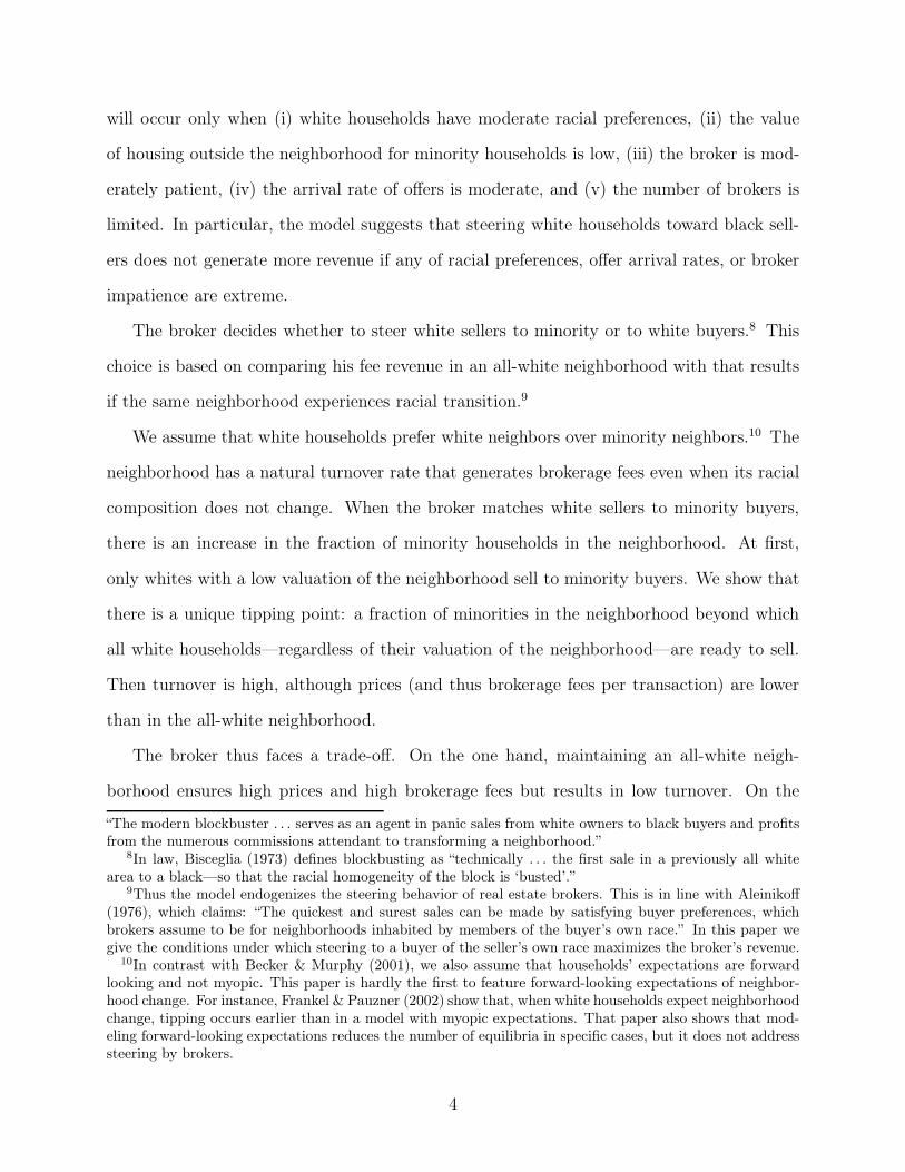
will occur only when (i) white households have moderate racial preferences, (ii) the value

of housing outside the neighborhood for minority households is low, (iii) the broker is mod-

erately patient, (iv) the arrival rate of offers is moderate, and (v) the number of brokers is

limited. In particular, the model suggests that steering white households toward black sell-

ers does not generate more revenue if any of racial preferences, offer arrival rates, or broker

impatience are extreme.

The broker decides whether to steer white sellers to minority or to white buyers.8 This

choice is based on comparing his fee revenue in an all-white neighborhood with that results

if the same neighborhood experiences racial transition.9

We assume that white households prefer white neighbors over minority neighbors.10 The

neighborhood has a natural turnover rate that generates brokerage fees even when its racial

composition does not change. When the broker matches white sellers to minority buyers,

there is an increase in the fraction of minority households in the neighborhood. At first,

only whites with a low valuation of the neighborhood sell to minority buyers. We show that

there is a unique tipping point: a fraction of minorities in the neighborhood beyond which

all white households—regardless of their valuation of the neighborhood—are ready to sell.

Then turnover is high, although prices (and thus brokerage fees per transaction) are lower

than in the all-white neighborhood.

The broker thus faces a trade-off. On the one hand, maintaining an all-white neigh-

borhood ensures high prices and high brokerage fees but results in low turnover. On the

“The modern blockbuster . . . serves as an agent in panic sales from white owners to black buyers and profitsfrom the numerous commissions attendant to transforming a neighborhood.”

8In law, Bisceglia (1973) defines blockbusting as “technically . . . the first sale in a previously all whitearea to a black—so that the racial homogeneity of the block is ‘busted’.”

9Thus the model endogenizes the steering behavior of real estate brokers. This is in line with Aleinikoff(1976), which claims: “The quickest and surest sales can be made by satisfying buyer preferences, whichbrokers assume to be for neighborhoods inhabited by members of the buyer’s own race.” In this paper wegive the conditions under which steering to a buyer of the seller’s own race maximizes the broker’s revenue.

10In contrast with Becker & Murphy (2001), we also assume that households’ expectations are forwardlooking and not myopic. This paper is hardly the first to feature forward-looking expectations of neighbor-hood change. For instance, Frankel & Pauzner (2002) show that, when white households expect neighborhoodchange, tipping occurs earlier than in a model with myopic expectations. That paper also shows that mod-eling forward-looking expectations reduces the number of equilibria in specific cases, but it does not addresssteering by brokers.

4

other hand, triggering a racial transition generates sequential patterns of transactions and

fees. Prices and turnover are initially low: high-valuation white households do not sell (low

turnover) and white households expect a neighborhood change (low prices). But when the

neighborhood reaches its tipping point, turnover increases and the broker realizes high rev-

enues. After the transition, however, turnover and prices decline to levels below those for an

all-white neighborhood. Given these dynamics, the broker’s incentive to trigger “white flight”

depends on whether or not the medium-term benefits of a large number of transactions offset

the lower transaction fees throughout the transition and in the long run.

We analyze how this trade-off depends on various parameters of the model, beginning

with white households’ racial preferences. In the case of strong racial aversion, the tipping

point would be reached rapidly but transaction prices would fall rapidly as well. When

racial preferences are weak, the tipping point is not reached until after a long period of time

characterized by low turnover and low transaction fees. It thus turns out that blockbusting

generates more revenue only for a bounded range of racial preferences.

Next we consider the effect of the broker’s impatience. Besides the usual time-discounting,

the broker’s impatience captures implicitly the likelihood that the broker no longer extracts

rents from a particular neighborhood in the future (though broker entry and exit are not

explicitly in the model.) Impatient brokers may be less inclined to practice blockbusting

because of the lower short-term brokerage fees (before the tipping point is reached). Moder-

ately patient brokers are willing to earn lower revenues at first as long as higher revenues can

be reasonably anticipated in the medium term (i.e., for some time after the tipping point).

Finally, brokers who are extremely patient do not benefit from blockbusting owing to the

lower long-term brokerage fees. Hence, there is a bounded range of broker discount rate for

which blockbusting generates more revenue.

We also take up the effect of minorities’ value of housing outside the neighborhood. When

this outside option is lower, blockbusting incentives are higher. When the options of minority

households improve, transaction prices (and brokerage fees) decrease. At the same time, the

5

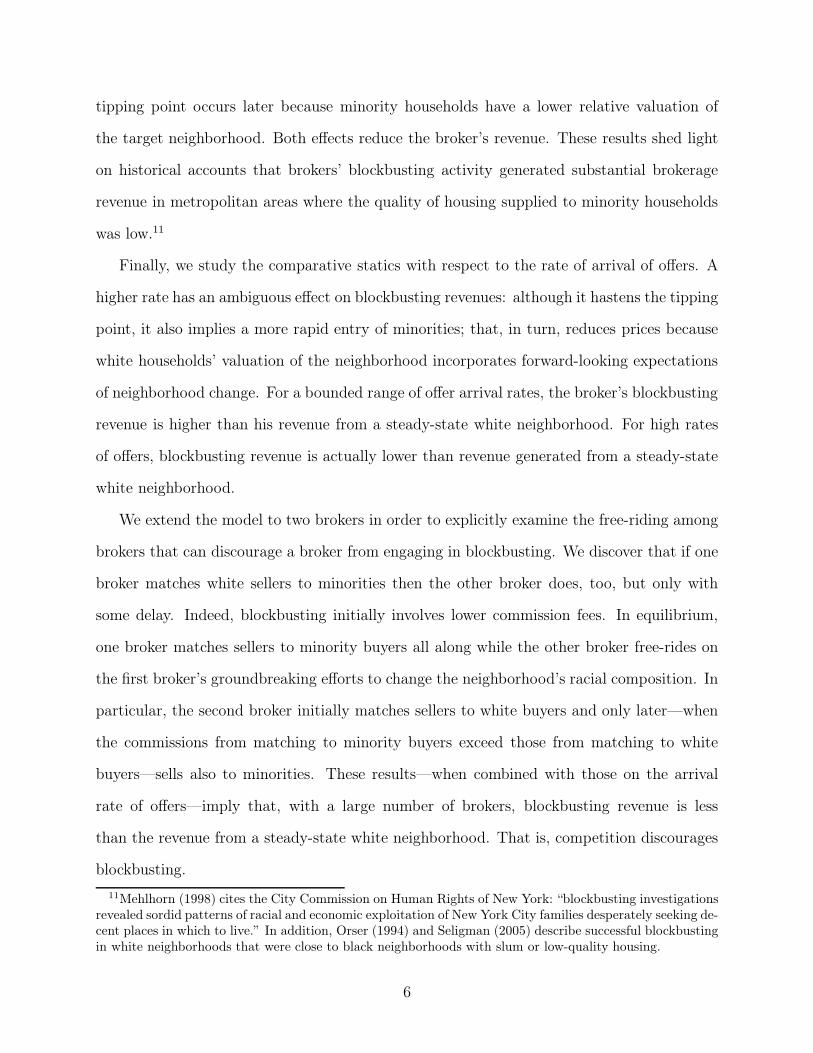
tipping point occurs later because minority households have a lower relative valuation of

the target neighborhood. Both effects reduce the broker’s revenue. These results shed light

on historical accounts that brokers’ blockbusting activity generated substantial brokerage

revenue in metropolitan areas where the quality of housing supplied to minority households

was low.11

Finally, we study the comparative statics with respect to the rate of arrival of offers. A

higher rate has an ambiguous effect on blockbusting revenues: although it hastens the tipping

point, it also implies a more rapid entry of minorities; that, in turn, reduces prices because

white households’ valuation of the neighborhood incorporates forward-looking expectations

of neighborhood change. For a bounded range of offer arrival rates, the broker’s blockbusting

revenue is higher than his revenue from a steady-state white neighborhood. For high rates

of offers, blockbusting revenue is actually lower than revenue generated from a steady-state

white neighborhood.

We extend the model to two brokers in order to explicitly examine the free-riding among

brokers that can discourage a broker from engaging in blockbusting. We discover that if one

broker matches white sellers to minorities then the other broker does, too, but only with

some delay. Indeed, blockbusting initially involves lower commission fees. In equilibrium,

one broker matches sellers to minority buyers all along while the other broker free-rides on

the first broker’s groundbreaking efforts to change the neighborhood’s racial composition. In

particular, the second broker initially matches sellers to white buyers and only later—when

the commissions from matching to minority buyers exceed those from matching to white

buyers—sells also to minorities. These results—when combined with those on the arrival

rate of offers—imply that, with a large number of brokers, blockbusting revenue is less

than the revenue from a steady-state white neighborhood. That is, competition discourages

blockbusting.

11Mehlhorn (1998) cites the City Commission on Human Rights of New York: “blockbusting investigationsrevealed sordid patterns of racial and economic exploitation of New York City families desperately seeking de-cent places in which to live.” In addition, Orser (1994) and Seligman (2005) describe successful blockbustingin white neighborhoods that were close to black neighborhoods with slum or low-quality housing.

6

The paper proceeds as follows. Section 2 presents the model. Section 3 solves the model

for the cases of no blockbusting (Section 3.1) and blockbusting (Section 3.2). Section 3.3

compares the revenues derived from racially transitioning and steady-state all-white neigh-

borhoods. Section 4 analyzes the effects of key parameters on the broker’s incentives to

blockbust: the effects of racial preferences, the broker’s discount rate, the minorities’ outside

option, and the arrival rate of offers. Section 5 presents the case of two brokers: one broker

free-rides on the other broker’s effort to introduce minority households in the neighborhood,

so a broker has less incentive to blockbust when there is another broker in the neighborhood.

Section 6 concludes. Proofs for all results are given in the Appendix.

2 Model

2.1 Neighborhood and Households

The neighborhood has a continuum of houses indexed by i ∈ [0, 1]. The residents of the

neighborhood are homeowning households; each house is owned by one household and each

household owns one house. For each house i, we let i also designate the owner, though the

identity may change over time. Homeowners are divided into two races, white (r = w) and

black (r = b).12 Whites can be either “relaxed” or “distressed”, as described in Section 3.2.

Time t ∈ [0,∞) is continuous. The household’s discount factor is β. The flow value for

whites living in the neighborhood is vw−e−ρb(t); here vw is the flow value of local amenities

and e is the household’s type, relaxed (e = 0) or distressed (e = ε).13 We use b(t) to denote

the fraction of black households that reduces the neighborhood’s flow value of utility by

ρb(t), where ρ is the strength of racial aversion.14 The flow value for blacks living in the

12We model two racial groups, which might also be Hispanics and African Americans. The importantassumption is that the incumbent race prefers neighbors of its own race.

13The shock be affects the utility of living in this particular neighborhood and may be due to job loss orfamily events. This feature is inspired by Albrecht, Anderson, Smith & Vroman (2007), who models—ina context different from racial segregation—households transitioning from a relaxed to a desperate stateaccording to a Poisson process.

14Bayer, Ferreira & McMillan (2007) provide estimates of the distribution of white households’ racial

7

neighborhood is vb, which is independent of the fraction of blacks in the neighborhood.15

At t = 0, all houses i ∈ [0, 1] of the neighborhood are owned by white households. At

time t, the density of relaxed white households is denoted R(t) while that of distressed white

households is denoted D(t). By construction, R(t) + D(t) + b(t) = 1. In a time interval

[t, t + dt), a relaxed (resp., distressed) white household becomes distressed (resp., relaxed)

with probability λ dt according to a Poisson process.

The discounted utility of living in the neighborhood for relaxed (resp., distressed) house-

holds is denoted V Rsw (resp., V D

sw).

Households enjoy a fixed16 flow value vlr when living outside the neighborhood, a value

that depends on race r ∈ {w, b}. The present discounted value when living outside the

neighborhood is Vlr = vlr/β.

2.2 Matching

The housing market has several frictions. First, there is a single broker through whom all

transactions must take place. Second, there are also frictions in matching the households

to the broker; this is realistic but we capture these frictions in a simple way: the broker

approaches anonymous homeowners in the hope of generating a sale but the households

cannot approach the broker. Though the broker can observe a buyer’s race, he cannot

observe whether a white buyer is relaxed or distressed.

A household living in the neighborhood is matched to a broker with probability δ dt in

a time interval [t, t + dt).17 The broker matches the household to a potential buyer. There

preferences using detailed transaction-level data in the San Francisco Bay area and assuming heterogeneityin households’ preferences.

15The model could be generalized so that blacks prefer black neighbors (or less distaste for black than forwhite neighbors); strongly similar implications would follow. If the preference of black households for whiteneighbors is greater than that of white households for white neighbors, then the tipping point is achieved att = 0 for b = 0.

16The value of housing outside the neighborhood will be fixed if two conditions obtain: (i) there is aninfinitely elastic supply of housing outside the neighborhood, so that the cost of housing is determined by themarginal cost of construction and land; and (ii) households are racially segregated outside the neighborhood.

17As Hsieh & Moretti (2003) point out, the vast majority of real estate transactions occur through a realestate broker. Yavaş (1992) presents a model where the real estate broker is an additional way to search for

8

exists an infinite measure of potential buyers—living outside the neighborhood—from which

the broker can choose. The broker observes the race of the seller but not her state (relaxed

or distressed). White households that move into the neighborhood are initially relaxed.

When a seller is matched to a potential buyer, the two households perform the transaction

only if doing so is mutually beneficial. The dummy variables τDb(t), τDw(t), τRb(t), and τRw(t)

are set equal to 1 or 0 to indicate whether or not, respectively, distressed whites (D) sell to

blacks (b), distressed whites (D) sell to whites (w), relaxed whites (R) sell to blacks (b), and

relaxed whites (R) sell to whites (w) at each time t ∈ [0,∞).

When a transaction occurs, buyer and seller split the surplus equally according to a

symmetric Nash bargaining mechanism. The respective transaction prices are denoted pDb(t),

pDw(t), pRb(t), and pRw(t), where {D,R} is the white seller’s state and {b, w} is the buyer’s

race.

The seller and the buyer each pay a brokerage fee of κ(p) that is linear in the transaction

price: κ(p) = αp + α0.18 The broker earns revenue π(t) dt per unit of time [t, t + dt). His

time discount factor is r, so the net present value of future revenues at time t is Π(t) =´ +∞

tπ(s)e−rs ds.

A key assumption is that the broker is able to choose the race of the potential buyer. In

other words, the broker chooses whether to match white sellers to black or to white buyers.

The broker’s strategy is assumed to take the following form. He starts by matching sellers

solely to white buyers from t = 0 to t = t, and he begins matching sellers solely to black

buyers from t = t to t = ∞. If the broker never matches a white seller to a black buyer,

then t = ∞.

Definition 1. An equilibrium is characterized by several factors: the fraction of black house-

holds b(t) in the neighborhood at time t ∈ [0,∞); the fraction of distressed D(t) and relaxed

housing and where the household’s and broker’s search efforts increase the probability δ of being matched toa buyer. In our model, the household’s search effort is zero and the broker’s search effort is fixed. However,this model could easily be extended to nonzero household search effort and endogenous broker search effort.

18We model the brokerage fee as a fixed percentage of the transaction price. This accords with Hsieh &Moretti (2003), who use the Consumer Expenditure Survey to show that the median commission fee paidwas 6.1% of the transaction price and exhibited little variance.

9

R(t) white households in the neighborhood at time t; indicator variables τDb(t), τDw(t),

τRb(t), and τRw(t), each set equal to 0 or 1; transaction prices pDb(t), pDw(t), pRb(t), and

pRw(t); and the broker’s strategy t. At equilibrium, the following statements hold.

• The broker’s strategy t is the earliest moment in time at which his present discounted

value of revenues when matching sellers to black buyers is higher than the present

discounted value of revenues when matching sellers to white buyers.

• Sellers and matched buyers accept mutually beneficial trades, and the two parties split

the transaction surplus equally.

Finally, we make one assumption regarding the initial fraction D(t = 0) of distressed

white households in the neighborhood.

Assumption 1. D(0) = λ/(δ + 2λ).

In the next section we show that this assumption guarantees a constant stock of distressed

white households in the all-white neighborhood.

3 Steady-State All-White Neighborhood versus Block-

busting

3.1 Steady-State All-White Neighborhood

This section derives households’ optimal behavior when the broker matches households with

white buyers only from t = 0 onward.19 Because the neighborhood is initially all-white, it

remains so—that is, b(t) = 0 for t ≥ 0. We shall derive the equilibrium turnover of the

neighborhood and the broker’s revenue.

19We show that Assumption 1 implies that the broker either (i) always matches sellers to white buyers(this section) or (ii) always matches sellers to black buyers (next section).

10

We demonstrate that the equilibrium of neighborhood depends on the size of the shock

ε to the flow value vw. Either (i) no trade occurs if ε is small or (ii) distressed households

sell to whites from outside the neighborhood if ε is above a threshold noted ε.

Case #1: No Transaction

Assume first that the shock ε is insufficient to make a distressed household willing to sell.

In this case, no trade occurs. Hence the Bellman equation for distressed whites’ value

of the neighborhood is βV Dsw = vw − ε + λ(V R

sw − V Dsw) and for relaxed whites is βV R

sw =

vw + λ(V Dsw − V R

sw). The respective value functions are V Rsw = [vw − ελ/(2λ + β)]/β and

V Dsw = [vw − ε− ελ/(2λ+ β)]/β, and the broker realizes no revenue.

Case #2: Relaxed Whites Sell

We assume therefore that ε is large enough to make transactions between distressed sellers

and white buyers mutually beneficial. We shall derive a formula for this minimum value of

ε after solving the model.

A transaction price pDw is acceptable to both seller and buyer if

Vlw + pDw − κ(pDw) ≥ V Dsw and V R

sw − pDw − κ(pDw) ≥ Vlw. (1)

The seller and the buyer each pay the broker a commission fee κ(pDw) = αpDw + α0. Hence

the broker receives 2κ(pDw) for each transaction. The transaction price pDw is such that the

transaction generates equal gains from trade for the seller and the buyer:

pDw =1

2

[

V Dsw − Vlw + V R

sw − Vlw

]

(2)

The smallest value of ε that makes trade mutually beneficial is denoted ε. This is the

11

minimum shock ε that satisfies

V Dsw − Vlw ≤ V R

sw − Vlw (3)

We now come to finding the values of living in the neighborhood. White households’

utilities satisfy the following equations:

V Rsw = vw dt+ e−β dt[(1− λ dt)V R

sw + λ dtV Dsw], (4)

V Dsw = (vw − ε) dt+ e−βdt

×[δ dt(Vlw + (1− α)pDw) + (1− δ dt)[(1− λ dt)V D

sw + λ dtV Rsw]

]. (5)

Now expanding equations (4) and (5) with respect to dt and neglecting terms in dt2 yields

βV Rsw = vw − λ[V R

sw − V Dsw], (6)

βV Dsw = vw − ε+ λ[V R

sw − V Dsw]

+ δ[Vlw + (1− α)pDw − α0 − V Dsw]. (7)

Equations (2), (6), and (7) thus determine the values V Rsw and V D

sw as well as the price pDw.

All three terms are decreasing in the shock ε. The Appendix shows that there is a minimum

shock ε such that condition (3) is satisfied. Above ε, a trade between a distressed white

seller and a white buyer is mutually beneficial; below ε, no such trade is beneficial.

Hence, when the broker matches white households to white buyers from t = 0 to t = ∞,

households’ optimal behavior depends on ε. For ε ≤ ε, no transaction takes place and so

no white household sells. For ε > ε, distressed white households sell (but relaxed white

households do not).

Proposition 1. Assume the broker chooses to match white households to white buyers from

t = 0 onward. When ε ≤ ε, no transactions occur. When ε > ε, distressed white households

12

sell but relaxed white households do not sell.

Neighborhood Composition

Assumption 1 implies that the fraction of distressed white households D(t) is constant as

long as the broker matches white sellers to white buyers only. To see this, note that the

change D(t+ dt)−D(t) in the number of distressed households in a time interval [t, t+ dt)

is the sum of three terms:

D(t+ dt)−D(t) = −δD(t) dt− λD(t) dt+ λR(t) dt

= −δD(t) dt− λD(t) dt+ λ(1−D(t)) dt.

The number of households moving into the neighborhood (who are initially relaxed) is

−δD(t) dt; the number of distressed households staying in the neighborhood and transition-

ing from the distressed to the relaxed state (see Section 3.2) is −λD(t) dt; and the number

of relaxed households staying in the neighborhood and becoming distressed is λR(t) dt.

Since R(0) = 1 − D(0), the assumption D(0) = λ/(δ + 2λ) implies that the number of

distressed households is constant: D(t + dt) − D(t) = 0. The number of transactions per

unit of time is then δ dt ·D = δλ/(δ + 2λ) · dt.

The Broker’s Revenue

The broker’s revenue in a period of time [t, t + dt) is the sum of the commission fees (for

buyer and seller) for each transaction δD(t) dt. At any equilibrium with transactions, only

distressed households sell. Let πss dt be the revenue made by the broker during each period

of time [t, t+dt); hence revenue πss is the number of transactions per unit of time multiplied

by the average total brokerage fee per transaction: πss = 2δD(αpDw + α0). Therefore, we

may write the present discounted value of revenues of the steady-state white neighborhood

13

Πss as

Πss =δ

rD[2κ(pDw)] =

2δ

rD[αpDw + α0].

The transaction price pDw is given by equation (2).

The Broker’s Optimal Strategy

In this section we solved the model when the broker matches sellers to white buyers only

for the period from t = 0 to t = ∞. The broker’s optimal strategy is either: (i) t = ∞,

matching white sellers to white buyers from t = 0 to t = ∞; or (ii) t = 0, matching whites

to blacks from t = 0 onward.

To see this point, observe that the present discounted revenue Π(t) depends on the frac-

tion D(t) of distressed households at time t and also on the fraction b(t) of black households

in the neighborhood at time t. The fractions of blacks, distressed, and relaxed households

are determined by the broker’s strategy and by the flows to and from the distressed state.

When the broker matches white sellers to white buyers, the fraction of blacks remains at

b(t) = 0 and the fraction of distressed households is also constant, D(t) = D(0). Therefore,

at any time t ≤ t, the broker faces the same incentives at t > 0 as he does at t = 0. From

this follows our proposition that the broker, from t = 0 onward, will either match sellers

to white buyers or match sellers to black buyers. In the next section we study the latter

strategy.

3.2 Blockbusting

This section shows that, if the broker matches white sellers to black buyers from t = 0

onward, then either white households do not sell or households’ behavior follows a tipping

point equilibrium. In such an equilibrium, distressed whites sell from t = 0 onward but

relaxed whites do not sell unless the fraction of blacks reaches the unique tipping point b.

A white household meets a buyer with probability δ dt in the time interval [t, t + dt). If

14

the household and the buyer agree to the sale, the result is a present discounted utility of

Vlw + pDb(t)−κ(pDb(t)). If seller and buyer do not agree to a sale, then the white household

receives a flow value (vw−e−ρb(t)) dt in [t, t+dt) and transitions from being relaxed (resp.,

distressed) to distressed (resp., relaxed) with probability λ dt.

When matched to a buyer, the distressed household’s value of living in the neighborhood

is20

V Dsw(t) = max

{Vlw + pDb(t)− κ(pDb(t)),

(vw − ε− ρb(t)) dt

+ e−β dt[(1− λ dt) · V Dsw(t + dt) + λ dt · V R

sw(t + dt)]}

(8)

with probability δ dt; when not matched to a buyer, the distressed household’s value of living

in the neighborhood is

V Dsw(t) = (vw − ε− ρb(t)) dt

+ e−β dt[(1− λ dt) · V Dsw(t+ dt) + λ dt · V R

sw(t+ dt)] (9)

with probability 1 − δ dt. Analogous statements hold for the valuation V Rsw(t) of the neigh-

borhood by a relaxed household (in which case the flow value is (vw − ρb(t)) dt instead of

(vw − ε− ρb(t)) dt).

Whites sell to buyers whenever there is a transaction price for which the trade is beneficial

to both seller and buyer. A transaction price pDb(t) leads to a mutually beneficial exchange

between a distressed white seller and a black buyer if both

Vlw + pDb(t)− κ(pDb(t)) ≥ V Dsw(t) and Vsb − pDb(t)− κ(pDb(t)) ≥ Vlb.

20For simplicity, we abuse notation slightly and let V Dsw(t) and V R

sw(t) denote random variables in additionto the expected utility of living in the neighborhood at t.

15

Similar conditions obtain for relaxed white households selling to black buyers.

The seller and the buyer share equally in the transaction surplus via the following sym-

metric Nash bargaining mechanism:21

pDb(t) =1

2

[

(V Dsw(t)− Vlw) + (Vsb − Vlb)

]

. (10)

Hence prices are a linear increasing function of the relative valuation Vsw(t) of the neighbor-

hood.

A seller–buyer transaction proceeds whenever (after transactions costs) the seller’s valu-

ation of the neighborhood is no greater than the buyer’s valuation:

V Dsw(t)− Vlw ≤ Vsb − Vlb. (11)

Given the price pDb(t) and the linearity of commission fees, condition (11) states that a

distressed (resp., relaxed) white homeowner sells to a black buyer whenever the former’s

valuation of the neighborhood does not exceed a certain threshold, V Dsw(t) ≤ Vsb − Vlb + Vlw

(resp., V Dsw(t) ≤ Vsb − Vlb + Vlw).

Because the broker is seeking black buyers for white sellers, the fraction of blacks in the

neighborhood is weakly increasing—that is, b(t′) ≥ b(t) for any t′ > t. Hence the value

functions V Dsw(t) and V R

sw(t) are decreasing with time. Therefore, a homeowner (distressed or

relaxed) who will sell at time t will also sell at any time t′ > t.

Because distressed households experience a negative valuation shock −ε dt ≤ 0 during

the time interval [t, t + dt), it follows that the value V Rsw(t) of the neighborhood for relaxed

whites is never less than the corresponding value V Dsw(t) for distressed whites. That is,

V Rsw(t) ≥ V D

sw(t). So if distressed whites do not sell then relaxed whites do not sell, either.

Finally, note that if distressed whites do not sell at t = 0 then (a) the fraction b(t) of

21The difference pDw−pDb(t) > 0 is the difference between the transaction price when the broker keeps theneighborhood white vs when he does blockbusting. Newspapers reported that families whose neighborhoodexperienced blockbusting sold “at a sizable loss” (Vitchek 1962), pDw − pDb(t) in the model.

16

black households in the neighborhood remains zero and (b) distressed whites do not sell at

any time t > 0.

We can now use these remarks to give a full characterization of household behavior at

equilibrium as follows.

Proposition 2. Assume that the broker matches white households to black buyers from t = 0

to t = ∞. Then there exist two values, ε∗ and ε∗∗, such that the following conditions hold.

• Case #1: For 0 < ε < ε∗, distressed whites do not sell.

• Case #2: For ε∗ < ε < ε∗∗: either (i) distressed whites do not sell at any time t, and

b(t) = 0 for t ∈ [0,∞); or (ii) distressed whites sell for t ∈ [0,∞) and relaxed whites

sell for t ≥ t, where t ∈ [0,∞).

• Case #3: For ε ≥ ε∗∗, distressed whites sell for t ∈ [0,∞) and relaxed whites sell for

t ≥ t, where t ∈ [0,∞).

Proof. See Appendix.

For values of ε ∈ [ε∗, ε∗∗], distressed whites sell at t = 0 only if other distressed whites

sell. Here ε∗ and ε∗∗ denote (respectively) the largest and smallest values of ε for which

selling at t = 0 is a dominated strategy for distressed whites.

We start with the determination of ε∗∗. Selling at t = 0 is a dominant strategy for

distressed whites if not selling at t = 0 is a dominated strategy. In turn, not selling is a

dominated strategy if there is any gain from selling to a black buyer when other distressed

white households do not sell:

[vw − ε(λ+ β)/(2λ+ β)

β

]

≤ Vsb − Vlb. (12)

The term [vw − ε(λ+ β)/(2λ+ β)]/β is the present value (for a distressed white household)

of staying in the neighborhood when no whites sell to blacks. Hence condition (12) defines

the minimum value of the shock ε∗∗ as the ε that satisfies (12) with equality.

17

t

Valu

ation

ofth

enei

ghborh

oodVsw(t)

Time t

Distressed White’s valuation V Dsw(t)

Relaxed White’s valuation V Rsw(t)

Threshold for selling to black buyers

This figure presents an example of determining the time needed to reach the tipping point t. Initially, att = 0, distressed whites sell to blacks; that is, V D

sw(t = 0)−V w

l+κ(pDb(t = 0)) ≤ Vsb−Vlb−κ(pDb(t = 0)). At

t = 0, relaxed whites do not sell. These households start selling as soon as they become indifferent betweenselling and not selling to black buyers, which determines the tipping point t. In the figure, this tipping pointis at the intersection of the downward-sloping dashed curve and the horizontal dotted line.The closed-form expressions of V R

sw(t) and V Dsw(t) are given in Section 3.2. The plots are generated by a

numerical simulation of the model using parameters provided in the Appendix.

Figure 1: Whites’ Valuation of the Neighborhood at Time t (Broker Matches White Sellersto Black Buyers)

18

Next we determine ε∗, which is the smallest value of the shock for which selling is a

dominated strategy when other distressed white households sell; as before, V Dsw(t) denotes

the value of living in the neighborhood at time t given that distressed white households sell.

This case prevails whenever no surplus is generated by a sale between a distressed white

seller and a black buyer (conditional on other white households selling):

V Dsw(0) ≥ Vsb − Vlb + Vlw. (13)

Hence, condition (13) defines the maximum value of the shock ε∗ as the ε that satisfies (13)

with equality.

The case ε < ε∗ (where no white household sells when matched to a potential buyer) is

of little interest, as it yields no revenue for the broker and no change in the neighborhood’s

racial composition. This explains our second assumption.

Assumption 2. ε ≥ ε∗.

Determination of the Unique Tipping Point

The second important result we show is that, in an equilibrium where white households sell

to black buyers, the tipping point b is unique.

Our derivation proceeds as follows. First, at the tipping point, white sellers are indifferent

between selling and not selling; thus the value of the neighborhood (relative to living outside

it) should be the same for both sellers and buyers. Second, we notice that the value function

is continuous at any time t—in particular, at the tipping point t. We can therefore derive

households’ value of living in the neighborhood at the tipping point by using the closed-form

expression for the value function at any time t after the tipping point.

The Bellman equation for valuing the neighborhood at time t ≥ t after tipping is given

19

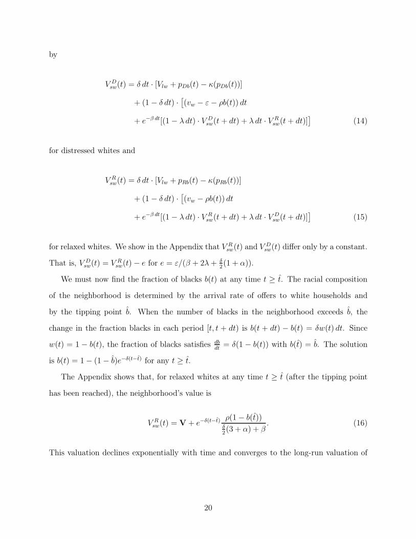
by

V Dsw(t) = δ dt · [Vlw + pDb(t)− κ(pDb(t))]

+ (1− δ dt) ·[(vw − ε− ρb(t)) dt

+ e−β dt[(1− λ dt) · V Dsw(t + dt) + λ dt · V R

sw(t+ dt)]]

(14)

for distressed whites and

V Rsw(t) = δ dt · [Vlw + pRb(t)− κ(pRb(t))]

+ (1− δ dt) ·[(vw − ρb(t)) dt

+ e−β dt[(1− λ dt) · V Rsw(t + dt) + λ dt · V D

sw(t+ dt)]]

(15)

for relaxed whites. We show in the Appendix that V Rsw(t) and V D

sw(t) differ only by a constant.

That is, V Dsw(t) = V R

sw(t)− e for e = ε/(β + 2λ+ δ2(1 + α)).

We must now find the fraction of blacks b(t) at any time t ≥ t. The racial composition

of the neighborhood is determined by the arrival rate of offers to white households and

by the tipping point b. When the number of blacks in the neighborhood exceeds b, the

change in the fraction blacks in each period [t, t + dt) is b(t + dt) − b(t) = δw(t) dt. Since

w(t) = 1 − b(t), the fraction of blacks satisfies dbdt

= δ(1 − b(t)) with b(t) = b. The solution

is b(t) = 1− (1− b)e−δ(t−t) for any t ≥ t.

The Appendix shows that, for relaxed whites at any time t ≥ t (after the tipping point

has been reached), the neighborhood’s value is

V Rsw(t) = V + e−δ(t−t) ρ(1− b(t))

δ2(3 + α) + β

. (16)

This valuation declines exponentially with time and converges to the long-run valuation of

20

an all-black neighborhood:

V Rsw(t = ∞) = V =

δ[1−α2

(Vsb − Vlb)−1+α2Vlw

]+ vw − ρ− λe

β + δ2(1 + α)

(17)

as t→ ∞ (derived in the Appendix).

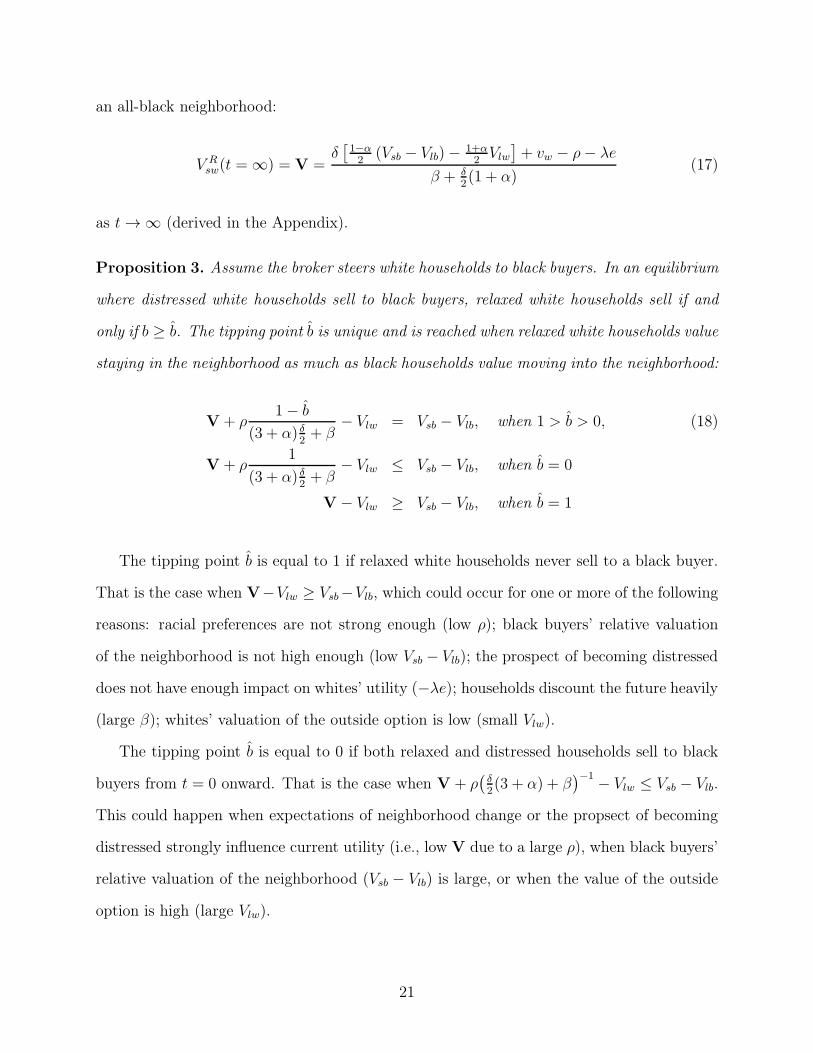
Proposition 3. Assume the broker steers white households to black buyers. In an equilibrium

where distressed white households sell to black buyers, relaxed white households sell if and

only if b ≥ b. The tipping point b is unique and is reached when relaxed white households value

staying in the neighborhood as much as black households value moving into the neighborhood:

V + ρ1− b

(3 + α) δ2+ β

− Vlw = Vsb − Vlb, when 1 > b > 0, (18)

V + ρ1

(3 + α) δ2+ β

− Vlw ≤ Vsb − Vlb, when b = 0

V − Vlw ≥ Vsb − Vlb, when b = 1

The tipping point b is equal to 1 if relaxed white households never sell to a black buyer.

That is the case when V−Vlw ≥ Vsb−Vlb, which could occur for one or more of the following

reasons: racial preferences are not strong enough (low ρ); black buyers’ relative valuation

of the neighborhood is not high enough (low Vsb − Vlb); the prospect of becoming distressed

does not have enough impact on whites’ utility (−λe); households discount the future heavily

(large β); whites’ valuation of the outside option is low (small Vlw).

The tipping point b is equal to 0 if both relaxed and distressed households sell to black

buyers from t = 0 onward. That is the case when V + ρ(δ2(3 + α) + β

)−1

− Vlw ≤ Vsb − Vlb.

This could happen when expectations of neighborhood change or the propsect of becoming

distressed strongly influence current utility (i.e., low V due to a large ρ), when black buyers’

relative valuation of the neighborhood (Vsb − Vlb) is large, or when the value of the outside

option is high (large Vlw).

21

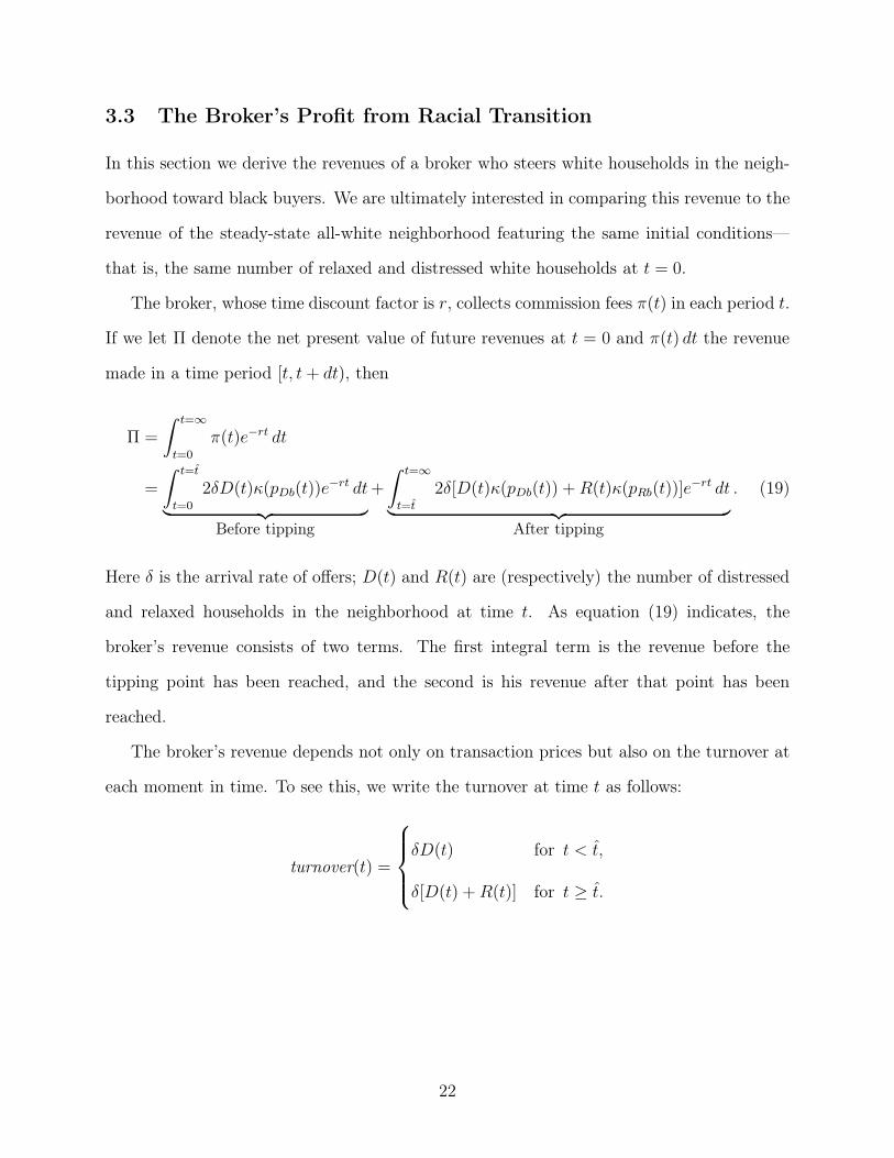
3.3 The Broker’s Profit from Racial Transition

In this section we derive the revenues of a broker who steers white households in the neigh-

borhood toward black buyers. We are ultimately interested in comparing this revenue to the

revenue of the steady-state all-white neighborhood featuring the same initial conditions—

that is, the same number of relaxed and distressed white households at t = 0.

The broker, whose time discount factor is r, collects commission fees π(t) in each period t.

If we let Π denote the net present value of future revenues at t = 0 and π(t) dt the revenue

made in a time period [t, t+ dt), then

Π =

ˆ t=∞

t=0

π(t)e−rt dt

=

ˆ t=t

t=0

2δD(t)κ(pDb(t))e−rt dt

︸ ︷︷ ︸

Before tipping

+

ˆ t=∞

t=t

2δ[D(t)κ(pDb(t)) +R(t)κ(pRb(t))]e−rt dt

︸ ︷︷ ︸

After tipping

. (19)

Here δ is the arrival rate of offers; D(t) and R(t) are (respectively) the number of distressed

and relaxed households in the neighborhood at time t. As equation (19) indicates, the

broker’s revenue consists of two terms. The first integral term is the revenue before the

tipping point has been reached, and the second is his revenue after that point has been

reached.

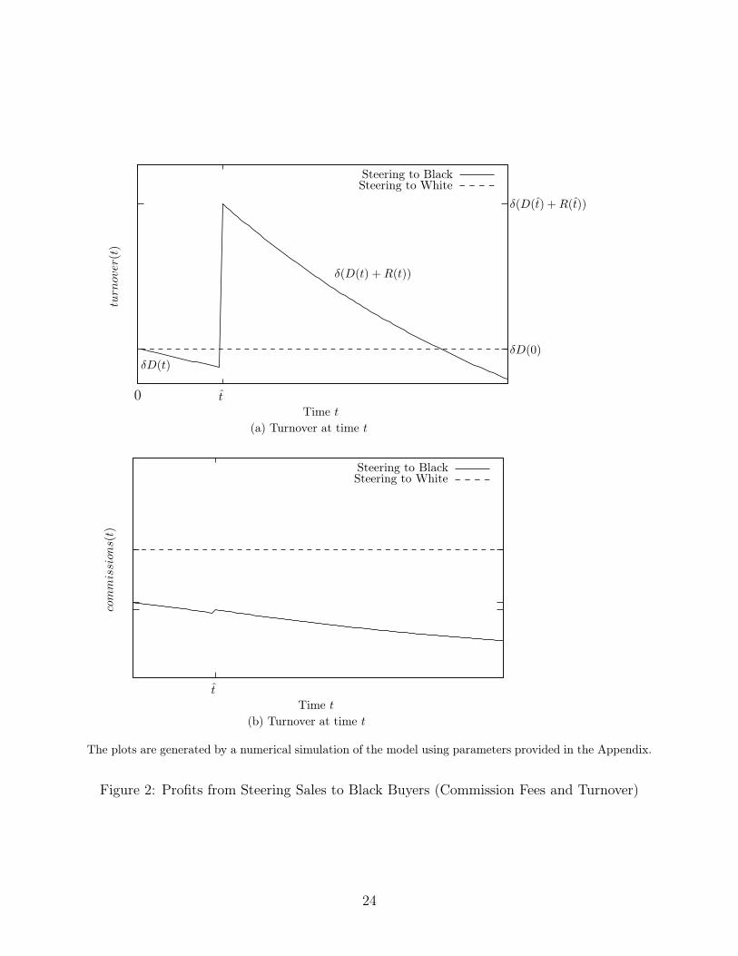
The broker’s revenue depends not only on transaction prices but also on the turnover at

each moment in time. To see this, we write the turnover at time t as follows:

turnover(t) =

δD(t) for t < t,

δ[D(t) +R(t)] for t ≥ t.

22

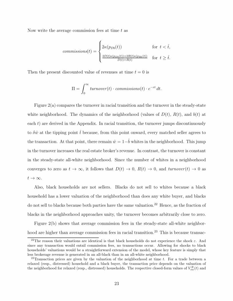
Now write the average commission fees at time t as

commissions(t) =

2κ(pDb(t)) for t < t,

2D(t)κ(pDb(t))+2R(t)κ(pRb(t))D(t)+R(t)

for t ≥ t.

Then the present discounted value of revenues at time t = 0 is

Π =

ˆ

∞

0

turnover(t) · commissions(t) · e−rt dt.

Figure 2(a) compares the turnover in racial transition and the turnover in the steady-state

white neighborhood. The dynamics of the neighborhood (values of D(t), R(t), and b(t) at

each t) are derived in the Appendix. In racial transition, the turnover jumps discontinuously

to δw at the tipping point t because, from this point onward, every matched seller agrees to

the transaction. At that point, there remain w = 1−b whites in the neighborhood. This jump

in the turnover increases the real estate broker’s revenue. In contrast, the turnover is constant

in the steady-state all-white neighborhood. Since the number of whites in a neighborhood

converges to zero as t → ∞, it follows that D(t) → 0, R(t) → 0, and turnover(t) → 0 as

t→ ∞.

Also, black households are not sellers. Blacks do not sell to whites because a black

household has a lower valuation of the neighborhood than does any white buyer, and blacks

do not sell to blacks because both parties have the same valuation.22 Hence, as the fraction of

blacks in the neighborhood approaches unity, the turnover becomes arbitrarily close to zero.

Figure 2(b) shows that average commission fees in the steady-state all-white neighbor-

hood are higher than average commission fees in racial transition.23 This is because transac-

22The reason their valuations are identical is that black households do not experience the shock ε. Andsince any transaction would entail commission fees, no transactions occur. Allowing for shocks to blackhouseholds’ valuations would be a straightforward extension of the model, whose key feature is simply thatless brokerage revenue is generated in an all-black than in an all-white neighborhood.

23Transaction prices are given by the valuation of the neighborhood at time t. For a trade between arelaxed (resp., distressed) household and a black buyer, the transaction price depends on the valuation ofthe neighborhood for relaxed (resp., distressed) households. The respective closed-form values of V R

sw(t) and

23

t0

turnover(t)

Time t

δD(t)

δ(D(t) +R(t))

δD(0)

δ(D(t) +R(t))

Steering to BlackSteering to White

(a) Turnover at time t

t

commissions(t)

Time t

Steering to BlackSteering to White

(b) Turnover at time t

The plots are generated by a numerical simulation of the model using parameters provided in the Appendix.

Figure 2: Profits from Steering Sales to Black Buyers (Commission Fees and Turnover)

24

tt0

π(t)=

commissions(t)·turnover(t)

Time t

Racial Transition π(t)Steady-State White πss

The plot is generated by a numerical simulation of the model using parameters provided in the Appendix.

Figure 3: Profits from Steering Sales to Black Buyers (Broker’s Revenue at Time t)

tion prices in the steady-state all-white neighborhood are higher than the average transaction

prices in racial transition. Once the tipping point is reached, white households expect in-

creasing numbers of black households in the neighborhood.24 There is a discontinuous jump

in the average commission fees at the tipping point; indeed, that is when relaxed whites start

accepting sales to blacks. These exchanges are transacted at higher prices than are those

between black buyers and distressed white sellers.

Comparing parts (a) and (b) of Figure 2 clearly shows that the real estate broker can

obtain higher revenue from a neighborhood in racial transition if the increased turnover

around the tipping point compensates for the lower average commission fees. This dynamic

is shown in Figure 3, which plots the instantaneous revenue π(t) of the real estate broker

at each moment in time. For the neighborhood in racial transition, the broker’s revenue is

lower before the tipping point. In the figure, revenue π(t) jumps above the revenue for the

V Dsw(t) before and after the tipping point are given in the Appendix (see the proof of Proposition 3 and

Lemma 2.24Before the tipping point, the number of blacks is b(t) =

´ t

0 δD(s) ds (see Appendix for the closed form

of this expression). After the tipping point, the number of blacks is b(t) = 1− (1− b)e−δ(t−t).

25

case of the all-white neighborhood at the tipping point, and it remains above that revenue

for the time period [t, t]. At t, the real estate broker begins to generate less revenue in the

racially transitioning neighborhood than in a steady-state all-white neighborhood.

4 Implications of the Model for the Profits from Racial

Transition

4.1 Racial Preferences

Racial preferences ρ have two effects on the broker’s blockbusting revenue. First, a higher

ρ (greater aversion) tends to lower the tipping point, which in turn raises broker revenue;

this is the tipping point effect. Second, a higher ρ reduces transaction prices (and hence

commission fees); this is the price effect, which lowers the broker’s revenue.

The tipping point effect is illustrated in Figure 4(a), where the tipping point is plotted

as a function of ρ. For values of ρ below ρ, the tipping point is b = 1 and only distressed

whites sell to black households at any time t. In this case, the neighborhood’s turnover and

the commission fees are lower than in the steady-state all-white neighborhood; therefore,

the broker’s revenue is lower when steering sellers to black buyers than to white buyers.

For higher values of ρ, the tipping point becomes b < 1. Figure 4(b) shows a case where,

at ρ = ρ1, the present discounted value (p.d.v.) of broker revenue is higher in a racially

transitioning neighborhood than in an all-white steady-state neighborhood (in the figure,

revenue at time t is depicted by the solid line). An increase from ρ1 to ρ2 lowers the tipping

point b > 0, which increases the broker’s p.d.v. of revenue from steering sellers to black

buyers. However, the attendant decline in prices will decrease that p.d.v. The new curve

of revenue at time t is depicted by the dashed line. The effect of ρ on total revenues is

ambiguous because it depends on which of these two effects dominates.

For values of ρ above ρ, the tipping point is b = 0 (see Figure 4(a)). In that case, the

26

1

0ρρ

Tip

pin

gpoin

tb

Racial preference ρ

b(ρ)

(a) The tipping point and racial preferences

t1t2

Rev

enue

at

tim

et

Time t

Revenue, ρ1Revenue, ρ2 > ρ1

Revenue, ρ3 > ρ > ρ2Revenue, Steering to Whites

(b) Revenue at time t and racial preferences

The plots are generated by a numerical simulation of the model using parameters provided in the Appendix.

Figure 4: Racial Preferences and (a) the Tipping Point, (b) Revenue at Time t

27

ρmaxρρmin

P.d

.v.

ofre

ven

ue

at

tim

e0

Racial preference ρ

Revenue, Steering to BlackRevenue, Steering to White

The plot is generated by a numerical simulation of the model using parameters provided in the Appendix.

Figure 5: Racial Preferences ρ and the Profits from Steering to Black Buyers

only effect is the price effect of ρ. This is illustrated in Figure 4(b) as ρ goes from ρ2 to

ρ3. The value ρ3 is greater than ρ. At ρ3, the only effect of an increase in ρ is a decline in

average prices (and hence in average commission fees), so at this point, too, there is only a

price effect. In short, the present discounted value of revenues from steering to black buyers

declines with increasing ρ.

These findings are summarized in Figure 5, which plots the present discounted value of

the broker’s revenue at time t = 0 as a function of racial preferences ρ. The dashed line is

the p.d.v. of the broker’s revenue in the steady-state all-white neighborhood, which is inde-

pendent of racial preferences. If the tipping point is b = 0 (ρ > ρ), then the broker’s revenue

is a decreasing function of racial preferences ρ. In this case, the price effect dominates. We

show that revenue is a linear decreasing function of ρ for ρ ≥ ρ.

Proposition 4. Profit is higher in the all-white neighborhood than in blockbusting for ρ = 0

and for ρ → ∞. Let ρmin and ρmax denote, respectively, the least and most racial aversion

for which broker revenue is greater under white flight than in a steady-state all-white neigh-

28

borhood. Then 0 < ρmin < ρmax < ∞. Profit is linear and decreasing for ρ ≥ ρ, where ρ is

the weakest level of racial preferences for which t = b = 0.

For ρ ≤ ρ, the effect of an increase in ρ on broker revenue is ambiguous because the

tipping point effect and the price effect are opposed: the former increases revenue whereas

the latter reduces it. Numerical simulations, as graphed in Figure 5, suggest that the tipping

point effect dominates the price effect for ρ ≤ ρ; this implies that, at time t = 0, the p.d.v.

Π of broker revenue is an increasing function of racial preferences ρ for ρ ≤ ρ.

4.2 The Broker’s Discount Rate

The broker’s discount rate r determines the relative weight given to revenues at each stage

of the neighborhood’s racial transition from all white to all black. Figure 3 and Section 3.2

describe these three stages. From t = 0 to the tipping point t = t, the broker’s revenue

π(t) is less when steering sellers to black than to white buyers. For t ∈ [t, t], the real estate

broker can make more revenue by steering sellers to black buyers. But for t ≥ t, steering to

blacks once again yields lower π(t).

A high time discount rate r (i.e., an impatient broker) gives greater weight to early

revenues π(t), t ≤ t, than to medium-term revenues, t ∈ [t, t], and long-term revenues, t ≥ t.

Conversely, a low time discount rate r (i.e., a patient broker) gives greater weight to long-term

revenues than to medium- and short-term revenues. The discount rate r thus determines a

broker’s incentive to blockbust, as is stated formally in the following proposition.

Proposition 5. If the tipping point is b > 0, then there are two values (r > 0 and r > 0)

of the time discount factor such that, when r /∈ [r; r], the p.d.v. of broker revenue Π =´

∞

0π(t)e−rt dt when steering to blacks is less than the p.d.v. of revenue π

ss/r when steering

to whites.

If the tipping point is b = 0, then a broker earns more revenue from steering to black than

to white buyers. That is, there exists a finite r such that the p.d.v. of revenues from steering

29

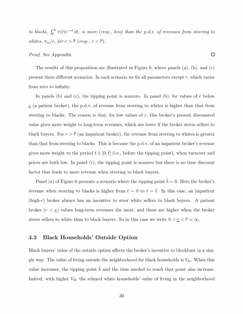
to blacks,´

∞

0π(t)e−rt dt, is more (resp., less) than the p.d.v. of revenues from steering to

whites, πss/r, for r > r (resp., r < r).

Proof. See Appendix.

The results of this proposition are illustrated in Figure 6, where panels (a), (b), and (c)

present three different scenarios. In each scenario we fix all parameters except r, which varies

from zero to infinity.

In panels (b) and (c), the tipping point is nonzero. In panel (b), for values of r below

r (a patient broker), the p.d.v. of revenue from steering to whites is higher than that from

steering to blacks. The reason is that, for low values of r, this broker’s present discounted

value gives more weight to long-term revenues, which are lower if the broker steers sellers to

black buyers. For r > r (an impatient broker), the revenue from steering to whites is greater

than that from steering to blacks. This is because the p.d.v. of an impatient broker’s revenue

gives more weight to the period t ∈ [0, t] (i.e., before the tipping point), when turnover and

prices are both low. In panel (c), the tipping point is nonzero but there is no time discount

factor that leads to more revenue when steering to black buyers.

Panel (a) of Figure 6 presents a scenario where the tipping point b = 0. Here the broker’s

revenue when steering to blacks is higher from t = 0 to t = t. In this case, an impatient

(high-r) broker always has an incentive to steer white sellers to black buyers. A patient

broker (r < r) values long-term revenues the most, and these are higher when the broker

steers sellers to white than to black buyers. So in this case we write 0 < r < r = ∞.

4.3 Black Households’ Outside Option

Black buyers’ value of the outside option affects the broker’s incentive to blockbust in a sim-

ple way. The value of living outside the neighborhood for black households is Vlb. When this

value increases, the tipping point b and the time needed to reach that point also increase.

Indeed, with higher Vlb, the relaxed white households’ value of living in the neighborhood

30

r

P.d

.v.

ofre

ven

ue

at

tim

e0

Broker’s discount factor r

Revenue, Steering to BlackRevenue, Steering to White

(a) Case 1: Tipping point is zero, π(0) > πss. One intersection

rr

P.d

.v.

ofre

ven

ue

at

tim

e0

Broker’s discount factor r

Revenue, Steering to BlackRevenue, Steering to White

(b) Case 2: Tipping point is nonzero, π(0) < πss. Two intersections.

P.d

.v.

ofre

ven

ue

at

tim

e0

Broker’s discount factor r

Revenue, Steering to BlackRevenue, Steering to White

(c) Case 3: Tipping point is nonzero, π(t) < πss. No intersection.

The plots are generated by a numerical simulation of the model using parameters provided in the Appendix.

Figure 6: Broker’s Discount Factor r and the Profits from Steering to Black Buyers

31

needs to decline by a larger amount in order to reach the time t at which selling to blacks

yields more revenue than does selling to whites. Note also that, when Vlb increases, trans-

action prices in the neighborhood decline. Hence, the p.d.v. of future revenues is decreasing

in Vlb. Formally, we have the following result.

Proposition 6. Transaction prices are a decreasing function of black households’ outside

option; that is, dpDb(t)/dVlb < 0 and dpRb(t)/dVlb < 0. The tipping point is an increasing

function of black households’ outside option; that is, db/dVsb > 0 and dt/dVsb > 0.

The revenue from matching white sellers to black buyers is a decreasing function of blacks’

valuation of housing outside the neighborhood. There is a value Vlb such that, for Vlb < Vlb,

steering white sellers to black buyers leads to more revenue than does steering them to white

buyers.

Proof. See Appendix.

4.4 Arrival Rate of Offers

The rate δ of arrival of offers has an ambiguous effect on the broker’s blockbusting revenue.

In the first place, a higher arrival rate decreases the time t required to reach the tipping point,

as more black households enter the neighborhood in each period [t, t+ dt); this increases the

broker’s revenue. The effect is illustrated in Figure 7(a), which shows the tipping point as a

function of δ while holding all other parameters constant. We use δ to denote the smallest

value of δ for which the tipping point is zero.

Second, a higher rate of arrival of offers lowers the tipping point b. Even though the

higher arrival rate increases the long-term valuation V = V Rsw(t = ∞) of living in an all-

black neighborhood, households have forward-looking expectations of neighborhood change

and so a higher δ has a greater (negative) impact on the current value of living in the

neighborhood. Thus, the tipping point b is lower when the arrival rate of offers is higher.

This effect, too, increases the broker’s blockbusting revenue.

32

However, a third effect of higher δ is one that reduces broker revenue. Namely, households’

forward-looking expectations of neighborhood change imply that the value of living in the

neighborhood is lower when black households enter the neighborhood more rapidly. Hence

transaction prices are lower when the arrival rate δ is higher.

These three effects are illustrated in Figure 7(b), which shows the revenue at time t for

three different values δ1 < δ2 < δ3. If the offer arrival rate increases from δ = δ1 to δ = δ2,

then the time until the tipping point is reduced from t1 to t2 and the neighborhood turnover

increases. However, as t → ∞, the revenue for δ = δ2 becomes lower than the revenue for

δ = δ1 because the fraction of whites in the neighborhood is smaller in the case of a high

arrival rate and so transaction prices are lower. At δ = δ3 the tipping point is zero and so

increasing δ can no longer affect the tipping point. However, increasing δ will continue to

induce falling transaction prices.

Figure 7(c) compares the present discounted value of the blockbusting revenue at t = 0 to

the present discounted value of revenues from an all-white neighborhood. In Section 3.1 we

showed that the p.d.v. of revenues in an all-white neighborhood is an increasing function of

the offer arrival rate δ. For very low values of δ, the p.d.v. of the revenue from blockbusting

is less than the p.d.v. of revenue from maintaining an all-white neighborhood. The reason is

that the time to reach the tipping point approaches infinity as the offer arrival rate approaches

zero. For very high values of δ, the p.d.v. of the blockbusting revenue is also less. This is

because, as δ → ∞, white households anticipate immediate neighborhood change and so

transaction prices are low. For values of δ ∈ [δmin, δmax], the revenue from blockbusting

revenue is higher than from the all-white neighborhood. The difference between these two

revenue levels decreases from δ onward, the point at which δ ceases to have any effect on the

tipping point.

33

δ

Tip

pin

gpoin

t

δ

Tipping point b(δ)

(a) Tipping point

t1t2

Rev

enue

at

tim

et

Time t

Blockbusting Revenue, δ1Blockbusting Revenue, δ2 > δ1

Blockbusting Revenue, δ3 > δ > δ2

(b) Revenue at time t for δ1 < δ2 < δ3

δmaxδδmin

P.d

.v.

ofre

ven

ue

at

tim

e0

Rate of arrival of offers δ

Revenue, Steering to BlackRevenue, Steering to White

(c) Revenue from blockbusting and from Steady-State All-WhiteNeighborhood for δ ∈ [0,∞)

The plots are generated by a numerical simulation of the model using parameters provided in the Appendix.

Figure 7: Offer Arrival Rate δ and the Profits from Steering to Black Buyers

34

5 Two Brokers

We now extend the model to feature two brokers. This creates a new aspect of the model in

that broker 1 and 2 interact strategically: one broker’s actions have an effect on the other

broker’s revenues and incentives. After presenting the equilibrium, we show that the second

broker free-rides on the blockbusting efforts of the first broker.

5.1 Extended Theoretical Framework

Following Section 2, we extend the model to include two brokers indexed by j = 1, 2. A

household of the neighborhood is matched to broker j = 1, 2 with probability δ dt in period

[t, t+ dt).

At time t, each broker decides whether to steer white sellers to black or to white buyers.

We focus on brokers’ monotonic strategies: for each j = 1, 2, we assume that broker j

matches sellers to white buyers for t ≤ tj and to black buyers for t ≥ tj . We denote by

Π2,w(t) (resp., Π2,b(t)) the present discounted value of broker 2’s future revenues from t to

∞ when he steers sellers exclusively to white (resp., black) buyers.

Definition 2. An equilibrium with two brokers is characterized by: the fraction of black

households b(t) in the neighborhood at time t ∈ [0,∞); the fraction of distressed D(t) and

relaxed R(t) white households in the neighborhood at time t; indicator variables τDb(t),

τDw(t), τRb(t), and τRw(t), each set equal to 1 (or 0) when there is (or is not) a transaction

between distressed or relaxed sellers and black or white buyers, as applies; the respective

transaction prices pDb(t), pDw(t), pRb(t), and pRw(t); and the strategy tj of each broker

j = 1, 2. At equilibrium, the following statements hold.

• The broker’s strategy tj is the earliest time at which his p.d.v. of revenues at time tj

when matching sellers to black buyers is greater than the p.d.v. of revenues (at that

time) when matching sellers to white buyers—given the other broker’s strategy t−j.

35

• Sellers and matched buyers accept mutually beneficial trades, and the two parties split

the transaction surplus equally.

5.2 Brokers’ Behavior at Equilibrium

We next turn to analyzing brokers’ behavior at equilibrium. Much as in the case with

one broker, in any equilibrium of the model we have either that all brokers steer sellers to

white buyers or that at least one of the two brokers starts steering sellers to black buyers at

t = 0. When both brokers steer sellers to white buyers, there is no change in the number of

distressed or relaxed whites (as a consequence of Assumption (1)). Hence the brokers have

the same incentives to steer sellers toward white (or black) buyers at t > 0 as they do at

t = 0.

What remains to be determined is the behavior of broker 2. By definition of the equilib-

rium, at every time t broker 2 compares the revenue from steering sellers to white buyers for

another interval of time, [t, t + dt), with the revenue from steering sellers to black buyers.

The broker thus compares the following two equations:

Π2,w(t) = max{π2,w(t) dt+ e−r dtΠ2,w(t+ dt),Π2,b(t)}, (20)

Π2,b(t) = π2,b(t) dt+ e−r dtΠ2,b(t+ dt). (21)

Equation (20) gives the present discounted value of revenues from the broker steering sellers

to white buyers until time t and then deciding to steer sellers to black buyers from time t

onward. Equation (21) gives the p.d.v. of broker revenue when steering to blacks from t

onward. Given broker 1’s equilibrium behavior, we use π2,w(t) dt (resp., π2,b(t) dt) to denote

the fees collected by broker 2 in [t, t+dt) when steering sellers to white (resp., black) buyers.

Intuitively, the point at equilibrium when broker 2 starts steering sellers to black buyers is

the t2 at which the brokerage fees π2,w(t2) and π2,b(t2) are equal. See Appendix for the proof,

which relies on deriving closed-form solutions for broker 2’s program to take the maximum

36

of equations (20) and (21). Thus we have our final proposition.

Proposition 7. In the case of two brokers, there can be one of two equilibria as follows.

1. (i) Both brokers match sellers to white buyers, and neither broker matches sellers to

black buyers; t1 = t2 = ∞.

2. (ii) One broker (say, broker 1) starts matching sellers to blacks at t = 0 (i.e., t1 =

0). The other broker (say, broker 2) matches sellers to white buyers as long as the

commission fees from doing so exceed those earned from matching to black buyers;

hence t2 is the earliest time at which both π2,w(t2) = π2,b(t2) and π2,w(t) ≥ π2,b(t) for

t ≤ t2.

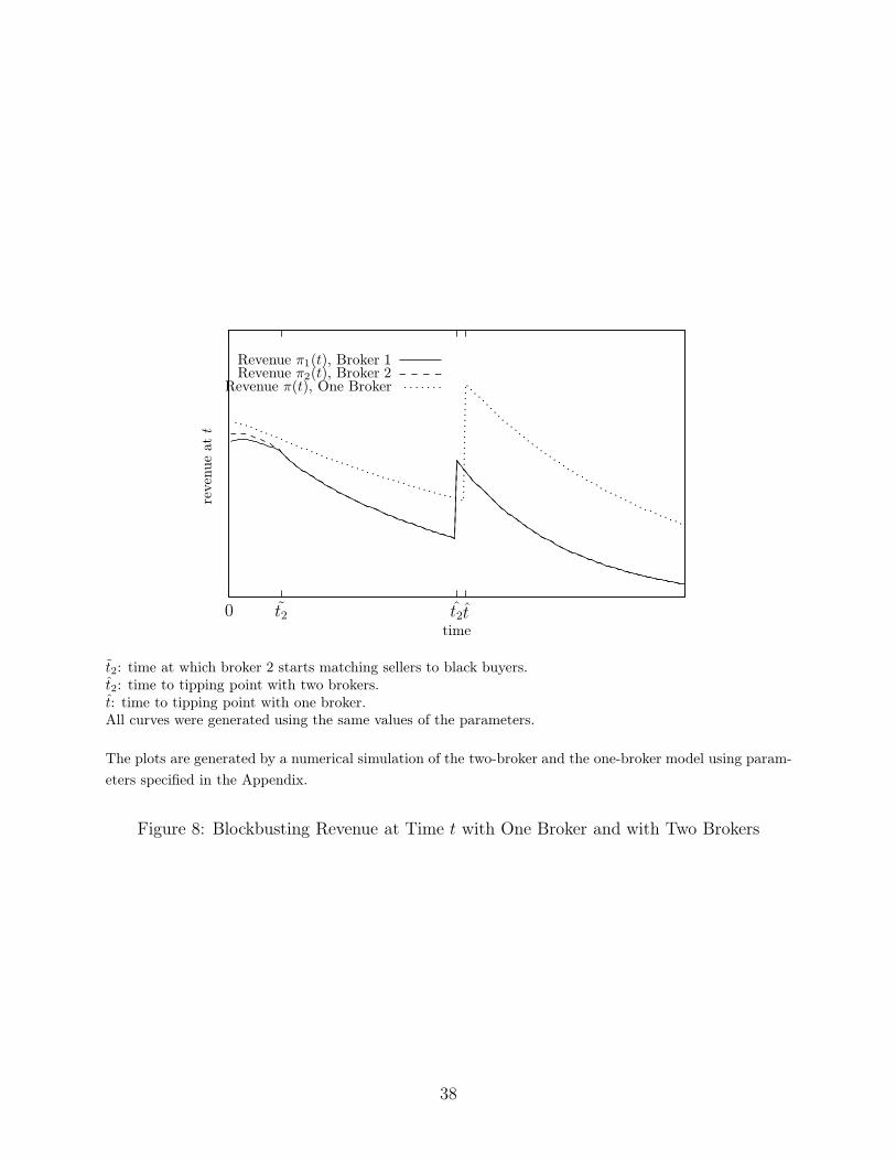
5.3 Blockbusting Revenue with One and Two Brokers

With two brokers, the offer arrival rate doubles from δ to 2δ. The impact of an increase in

this rate was described in Section 4.4; such an increase leads to a lower tipping point but

also to lower prices/commissions. In addition to these effects, with two brokers the strategic

behavior of the one who does not start blockbusting at t = 0 tends to lower the revenue of

the one who does engage in blockbusting at t = 0. Indeed, broker 2 generally starts matching

sellers to black buyers not at t = 0 but rather at t2 ≥ 0. However, if t ≥ t2 then broker 2

continues matching white sellers to black buyers.

Figure 8 shows the revenue at time t in the case of two brokers and in the case of one

broker. Here the equilibrium is such that broker 1 steers sellers to black buyers from t = 0

onward and broker 2 does so from t = t2 onward. The figure plots the revenue of broker 1

and broker 2 (π1(t) and π2(t), respectively) at time t; it also plots the revenue π(t) when

there is only one broker (but with the same values of the parameters).

37

tt2t20

reven

ue

att

time

Revenue π1(t), Broker 1Revenue π2(t), Broker 2

Revenue π(t), One Broker

t2: time at which broker 2 starts matching sellers to black buyers.t2: time to tipping point with two brokers.t: time to tipping point with one broker.All curves were generated using the same values of the parameters.

The plots are generated by a numerical simulation of the two-broker and the one-broker model using param-

eters specified in the Appendix.

Figure 8: Blockbusting Revenue at Time t with One Broker and with Two Brokers

38

5.4 Revenue and a Large Number of Brokers

Section 4.4 showed for high offer arrival rates that, as δ → ∞, blockbusting revenue becomes

less than the revenue from a steady-state all-white neighborhood.

Similarly, with a large number N of brokers, the rate of arrival of brokers is Nδ and,

as N → ∞, broker revenue is less from racially transitioning than from the steady-state

all-white neighborhoods. This dynamic is shown in Figure 7(c). Because N is large, the

tipping point becomes b = 0 (see Figure 7(a)). When δ increases for b = 0, prices decline as

the number of brokers increases and so the revenue of each individual broker declines.

6 Conclusion

This paper focuses on the ability and incentives of a real estate broker to change the equilib-

rium racial composition of a neighborhood. We show that the broker can turn an all-white

neighborhood into an all-black neighborhood if there are enough distressed white sellers to

which he can match black buyers. Once the neighborhood contains a threshold fraction of

black households, all white households (whether relaxed or distressed) sell and turnover is

high. The broker has a financial incentive to change a neighborhood’s racial composition if

doing so yields a greater present discounted value of revenues than does maintaining a stable

all-white neighborhood.

The mechanisms described here suggest that we adopt a nuanced view of the broker’s

incentives to steer sellers to black buyers. Neighborhoods where white households strongly

dislike black neighbors are, in fact, not the best candidates because prices in such neighbor-

hoods are significantly lower when households anticipate a large increase in the black popu-

lation. The broker refrains from blockbusting also in neighborhoods where white households

have no particular racial preference concerning their neighbors. Rather, the broker engages

in blockbusting only within a (limited) range of racial preference values (ρ) for which steer-

ing to black buyers leads to greater present discounted revenue. With respect to such racial

39

preferences, the United States District Court for the northern district of Illinois states:

Blockbusting and panic peddling are real estate practices in which brokers en-

courage owners to list their homes for sale by exploiting fears of racial change

within their neighborhood.25

Fears of racial change (i.e., racial preferences) are key to the blockbusting process. How-

ever, they lead to lower valuations of the neighborhood by white households and hence to

lower transaction prices and commissions. These effects may discourage blockbusting and

encourage brokers to steer sellers toward white buyers.

The model also demonstrates why an impatient broker is less likely to be a blockbuster—

namely, because of the initially lower fees generated thereby. Extremely high rates of arrival

of offers are also unlikely to encourage blockbusting because then both short- and long-

term transaction prices are lower. Extending the model to the case of two brokers indicates

that the second broker free-rides on the first broker’s initial blockbusting efforts. Finally,

blockbusting occurs only with a limited number of brokers. When there are too many brokers,

blockbusting incentives decline because then the offer arrival rate is high and so prices are

low.

More generally, this paper models a broker who can choose the market equilibrium in a

setting where social interactions among agents imply multiple equilibria. Hence the model

should have broader applicability and relevance beyond the issue of blockbusting and white

flight. Finally, because households’ expectations are forward looking, the model could also be

used to explain how a real estate broker can “gentrify” an all-black neighborhood by steering

black households toward white buyers.

25Pearson v. Edgar, 965 F. Supp. 1104, 1108–09 (N.D. Ill. 1997), cited in Mehlhorn (1998).

40

References

Albrecht, J., Anderson, A., Smith, E. & Vroman, S. (2007), ‘Opportunistic matching in the

housing market’, International Economic Review 48(2), 2007.

Aleinikoff, A. (1976), ‘Racial steering: The real estate broker and title viii’, Yale Law Journal

808(812).

Alesina, A. & Ferrara, E. L. (2000), ‘Participation in heterogeneous communities’, The Quar-

terly Journal of Economics 115(3), 847–904.

Bayer, P., Ferreira, F. & McMillan, R. (2007), ‘A unified framework for measuring preferences

for schools and neighborhoods’, Journal of Political Economy 115, 588–638.

Bayer, P., McMillan, R. & Rueben, K. S. (2004), ‘What drives racial segregation? new

evidence using census microdata’, Journal of Urban Economics 56(3), 514–535.

Becker, G. & Murphy, K. (2001), Social Markets: Market Behavior in a Social Environment,

Belknap-Harvard University Press.

Benabou, R. (1993), ‘Workings of a city: Location, education, and production’, The Quar-

terly Journal of Economics 108(3), 619–52.

Benabou, R. (1996), ‘Equity and efficiency in human capital investment: The local connec-

tion’, Review of Economic Studies 63(2), 237–64.

Bisceglia, J. G. (1973), ‘Blockbusting: Judicial and legislative response to real estate dealers’

excesses’, De Paul Law Review 818(22).

Blockbusting (1970), Vol. 59, Georgetown Law Journal, p. 170.

Boustan, L. P. (2007), ‘Black migration, white flight: The effect of black migration on

northern cities and labor markets’, The Journal of Economic History 67(02), 484–488.

41

Boustan, L. P. (2010), ‘Was postwar suburbanization “white flight”? evidence from the black

migration’, The Quarterly Journal of Economics 125(1), 417–443.

Boustan, L. P. & Margo, R. A. (2009), ‘Race, segregation, and postal employment: New

evidence on spatial mismatch’, Journal of Urban Economics 65(1).

Card, D., Mas, A. & Rothstein, J. (2008), ‘Tipping and the dynamics of segregation’, The

Quarterly Journal of Economics 123(1), 177–218.

Card, D. & Rothstein, J. (2007), ‘Racial segregation and the black-white test score gap’,

Journal of Public Economics 91(11-12), 2158–2184.

Clark, K. (1965), Dark Ghetto: Dilemmas of Social Power, Wesleyan University Press.

Courant, R. & Hilbert, D. (1989), Methods of Mathematical Physics, Vol. I-IV, Wiley.

Cutler, D. M. & Glaeser, E. L. (1997), ‘Are ghettos good or bad?’, The Quarterly Journal

of Economics 112(3), 827–72.

Easterly, W. (2009), ‘Empirics of strategic interdependence: The case of the racial tipping

point’, The B.E. Journal of Macroeconomics 9(1), 25.

Frankel, D. M. & Pauzner, A. (2002), ‘Expectations and the timing of neighborhood change’,

Journal of Urban Economics 51(2), 295–314.

Glassberg, S. S. (1972), ‘Legal control of blockbusting’, Urban Law Annual 145.

Gotham, K. F. (2002), Race, Real Estate, and Uneven Development, SUNY Press.

Grubb, W. (1982), ‘The flight to the suburbs of population and employment, 1960-1970’,

Journal of Urban Economics 11(3), 348–367.

Helper, R. (1969), Racial Policies and Practices of Real Estate Brokers, University of Min-

nesota Press, Minneapolis.

42

Hirsch, A. R. (1983), Making the second ghetto: race and housing in Chicago, 1940-1960,

Cambridge University Press, Cambridge.

Hsieh, C.-T. & Moretti, E. (2003), ‘Can free entry be inefficient? fixed commissions and

social waste in the real estate industry’, Journal of Political Economy 111(5), 1076–

1122.

Logan, J. R. & Stults, B. J. (2011), The persistence of segregation in the metropolis: New

findings from the 2010 census, Technical report, Russell Sage Foundation.

Mehlhorn, D. (1998), ‘A requiem for blockbusting: Law, economics and race-based real estate

speculation’, Fordham Law Review 67, 1145–1192.

Moskowitz, A. (1977), ‘The first amendment: A blockbuster’s best friend’, UMKC Law

Review .

Ondrich, J., Ross, S. & Yinger, J. (2003), ‘Now you see it, now you don’t: Why do real estate

agents withhold available houses from black customers?’, The Review of Economics and

Statistics 85(4), 854–873.

Orser, E. (1994), Blockbusting in Baltimore: The Edmondson Village Story, The University

Press of Kentucky.

Saiz, A. & Wachter, S. (2011), ‘Immigration and the neighborhood’, American Economic

Journal: Economic Policy 3(2), 169–88.

Schelling, T. C. (1969), ‘Models of segregation’, American Economic Review 59(2), 488–93.

Schelling, T. C. (1971), ‘Dynamic models of segregation’, Journal of Mathematical Sociology

1, 143–186.

Seligman, A. I. (2005), Block by Block: neighborhoods and public policy on Chicago’s West

Side, The University of Chicago Press.

43

Turner, M. A. & Mikelsons, M. (1992), ‘Patterns of racial steering in four metropolitan

areas’, Journal of Housing Economics 2(3), 199–234.

Vitchek, N. (1962), ‘Confessions of a blockbuster’, Saturday Evening Post.

Yavaş, A. (1992), ‘A simple search and bargaining model of real estate markets’, Real Estate

Economics 20(4), 533–548.

read:

44

Symbol Meaning

α Fraction of the price paid as commission fee by buyer and seller

δ Rate of arrival of offers

β Households’ time discount factor

r Broker’s time discount factor

κ(p) Brokerage fee

b(t) Fraction black in the neighborhood at time t

V Dsw(t), V

Rsw(t) Present value of the neighborhood at t for (distressed, relaxed) white households

Vsb Present value of the neighborhood at t for black households

vw + e− ρb(t) Flow value of the neighborhood in [t, t+ dt)

e Household’s type, relaxed (e = 0) or distressed (e = −ε)

ρ Disutility of an all-black neighborhood for white households

Vlw Value of living outside the neighborhood for whites

Vlb Value of living outside the neighborhood for blacks

vb Instantaneous utility of living in the neighborhood in [t, t+ dt) for blacks

π(t) Broker’s profit in [t, t + dt) from racially transitioning neighborhood

πss Broker’s profit from steady-state all-white neighborhood

Π Present value of broker’s revenue from racially transitioning neighborhood

Πss Present value of broker’s revenue from steady-state all-white neighborhood

b Tipping point (fraction of black households in the neighborhood

t Time to reach the tipping point

ρ Minimum racial preference for which b = 0 and t = 0

ε∗∗ Minimum ε for which selling is a dominant strategy (matched to blacks)

ε∗ Maximum ε for which selling is a dominated strategy (matched to blacks)

ε Minimum shock for which selling is an equilibrium (matched to whites)

Table 1: Glossary of Notation for One-Broker Model

45

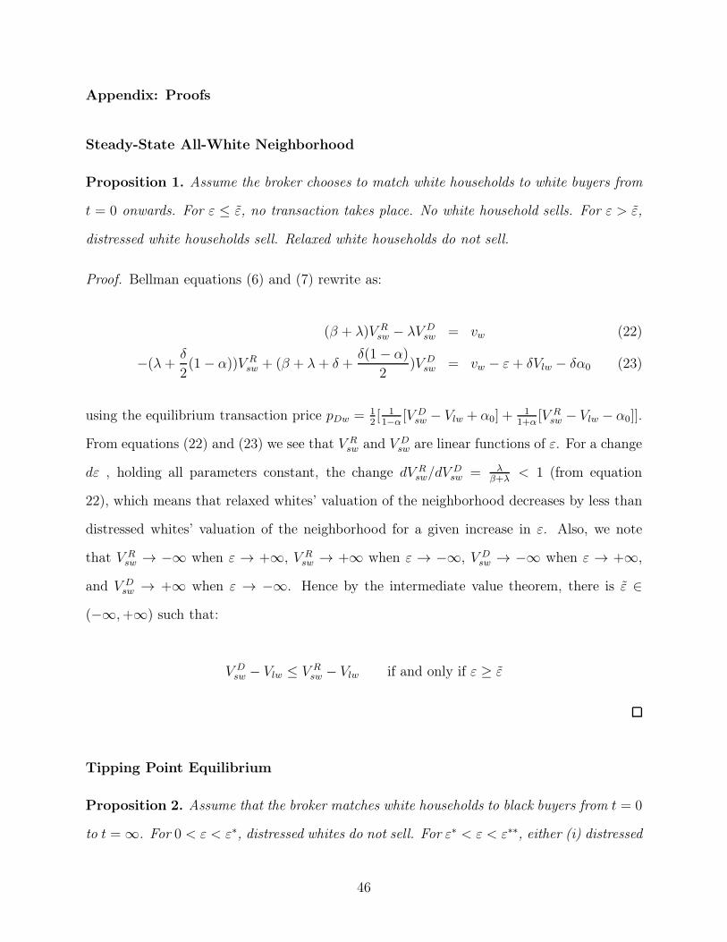
Appendix: Proofs

Steady-State All-White Neighborhood

Proposition 1. Assume the broker chooses to match white households to white buyers from

t = 0 onwards. For ε ≤ ε, no transaction takes place. No white household sells. For ε > ε,

distressed white households sell. Relaxed white households do not sell.

Proof. Bellman equations (6) and (7) rewrite as:

(β + λ)V Rsw − λV D

sw = vw (22)

−(λ+δ

2(1− α))V R

sw + (β + λ+ δ +δ(1− α)

2)V D

sw = vw − ε+ δVlw − δα0 (23)

using the equilibrium transaction price pDw = 12[ 11−α

[V Dsw − Vlw + α0] +

11+α

[V Rsw − Vlw − α0]].

From equations (22) and (23) we see that V Rsw and V D

sw are linear functions of ε. For a change

dε , holding all parameters constant, the change dV Rsw/dV

Dsw = λ

β+λ< 1 (from equation

22), which means that relaxed whites’ valuation of the neighborhood decreases by less than

distressed whites’ valuation of the neighborhood for a given increase in ε. Also, we note

that V Rsw → −∞ when ε → +∞, V R

sw → +∞ when ε → −∞, V Dsw → −∞ when ε → +∞,

and V Dsw → +∞ when ε → −∞. Hence by the intermediate value theorem, there is ε ∈

(−∞,+∞) such that:

V Dsw − Vlw ≤ V R

sw − Vlw if and only if ε ≥ ε

Tipping Point Equilibrium

Proposition 2. Assume that the broker matches white households to black buyers from t = 0

to t = ∞. For 0 < ε < ε∗, distressed whites do not sell. For ε∗ < ε < ε∗∗, either (i) distressed

46

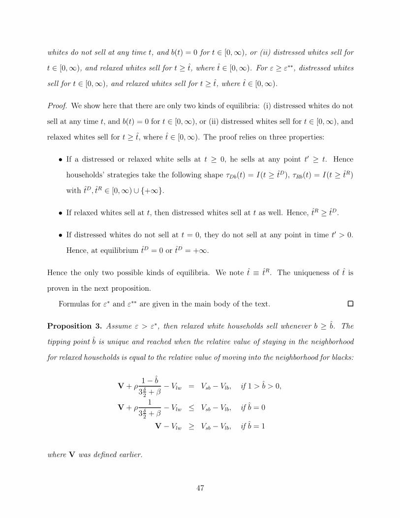
whites do not sell at any time t, and b(t) = 0 for t ∈ [0,∞), or (ii) distressed whites sell for

t ∈ [0,∞), and relaxed whites sell for t ≥ t, where t ∈ [0,∞). For ε ≥ ε∗∗, distressed whites

sell for t ∈ [0,∞), and relaxed whites sell for t ≥ t, where t ∈ [0,∞).

Proof. We show here that there are only two kinds of equilibria: (i) distressed whites do not

sell at any time t, and b(t) = 0 for t ∈ [0,∞), or (ii) distressed whites sell for t ∈ [0,∞), and

relaxed whites sell for t ≥ t, where t ∈ [0,∞). The proof relies on three properties:

• If a distressed or relaxed white sells at t ≥ 0, he sells at any point t′ ≥ t. Hence

households’ strategies take the following shape τDb(t) = I(t ≥ tD), τRb(t) = I(t ≥ tR)

with tD, tR ∈ [0,∞) ∪ {+∞}.

• If relaxed whites sell at t, then distressed whites sell at t as well. Hence, tR ≥ tD.

• If distressed whites do not sell at t = 0, they do not sell at any point in time t′ > 0.

Hence, at equilibrium tD = 0 or tD = +∞.

Hence the only two possible kinds of equilibria. We note t ≡ tR. The uniqueness of t is

proven in the next proposition.

Formulas for ε∗ and ε∗∗ are given in the main body of the text.

Proposition 3. Assume ε > ε∗, then relaxed white households sell whenever b ≥ b. The

tipping point b is unique and reached when the relative value of staying in the neighborhood

for relaxed households is equal to the relative value of moving into the neighborhood for blacks:

V + ρ1− b

3 δ2+ β

− Vlw = Vsb − Vlb, if 1 > b > 0,

V + ρ1

3 δ2+ β

− Vlw ≤ Vsb − Vlb, if b = 0

V − Vlw ≥ Vsb − Vlb, if b = 1

where V was defined earlier.

47

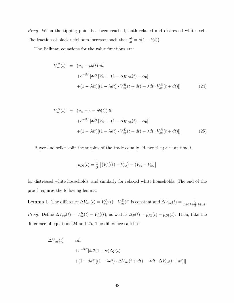
Proof. When the tipping point has been reached, both relaxed and distressed whites sell.

The fraction of black neighbors increases such that dbdt

= δ(1− b(t)).

The Bellman equations for the value functions are:

V Rsw(t) = (vw − ρb(t))dt

+e−βdt[δdt [Vlw + (1− α)pDb(t)− α0]

+(1− δdt)[(1− λdt) · V Rsw(t+ dt) + λdt · V D

sw(t+ dt)]] (24)

V Dsw(t) = (vw − ε− ρb(t))dt

+e−βdt[δdt [Vlw + (1− α)pDb(t)− α0]

+(1− δdt)[(1− λdt) · V Dsw(t+ dt) + λdt · V R

sw(t+ dt)]] (25)

Buyer and seller split the surplus of the trade equally. Hence the price at time t:

pDb(t) =1

2

[(V Dsw(t)− Vlw

)+ (Vsb − Vlb)

]

for distressed white households, and similarly for relaxed white households. The end of the

proof requires the following lemma.

Lemma 1. The difference ∆Vsw(t) = V Rsw(t)−V

Dsw(t) is constant and ∆Vsw(t) =

ε

β+2λ+ δ

2(1+α)

.

Proof. Define ∆Vsw(t) = V Rsw(t)− V D

sw(t), as well as ∆p(t) = pRb(t)− pDb(t). Then, take the

difference of equations 24 and 25. The difference satisfies:

∆Vsw(t) = εdt

+e−βdt[δdt(1− α)∆p(t)

+(1− δdt)[(1− λdt) ·∆Vsw(t + dt)− λdt ·∆Vsw(t + dt)]]

48

Noticing that ∆p(t) = 12∆Vsw(t), then

∆Vsw(t) = εdt

+e−βdt[δdt1− α

2∆Vsw(t)

+(1− δdt) · (1− 2λdt) ·∆Vsw(t + dt)]

Expanding ∆Vsw(t+ dt) = Vsw(t) +∂Vsw(t)

∂t· dt, e−βdt = 1− βdt, and neglecting terms in dt2:

β∆Vsw(t) = ε− (2λ+δ

2(1 + α))∆Vsw(t) +

∂∆Vsw(t)

∂t(26)

We assume that the value functions V Dsw and V R

sw stay finite over t ∈ [0,∞). Hence ∆Vsw(t)

does not diverge as t→ ∞. As β+2λ+ δ2(1+α) > 0, the only bounded solution to equation

26 is a constant:

∆Vsw(t) =ε

β + 2λ+ δ2(1 + α)

≡ e

This concludes the proof of the lemma.

The lemma allows us to finish the proof of proposition 3. Going back to the Bellman

equation of relaxed white households (equation 24), we use the lemma, V Dsw(t) = V R

sw(t)− e;

expand V Rsw(t+ dt) = V R

sw(t) +∂V R

sw(t)∂t

· dt, e−βdt = 1− βdt, and neglect terms in dt2. Then,

βV Rsw(t) = vw − ρb(t)

+δ

[

Vlw +1− α

2

[(V Rsw(t)− Vlw

)+ (Vsb − Vlb)

]− α0 − V R

sw(t)

]

+∂V R

sw(t)

∂t− λe

Noting ( δ2(1 + α) + β)V = δ

[Vlw + 1−α

2[−Vlw + (Vsb − Vlb)]− α0

]+ vw − ρ − λe, this leads

to the following differential equation for the value function:

∂V Rsw(t)

∂t− (

δ

2(1 + α) + β) · V R

sw(t) + (δ

2(1 + α) + β)V + ρ(1− b(t)) = 0 (27)

49

And note that V = limt→∞ V Rsw(t). To solve the first-order differential equation (27), define

a function ϕ(t) = V Rsw(t)e

−( δ2(1+α)+β)t. Then, this function satisfies a solvable first-order

equation.

ϕ′(t) = −((δ

2+ β)V + ρ(1− b(t))) · e−( δ

2(1+α)+β)t (28)

Interestingly, ϕ(∞) = 0, because the value functions of distressed and relaxed white V Rsw(t)

and V Dsw(t) are assumed bounded over t ∈ [0,∞) and e(

δ

2(1+α)+β)t → ∞ as t → ∞. Hence

the solution to equation 28 is ϕ(t) =´

∞

t(( δ

2+ β)V + ρ(1 − b(s))) · e−( δ

2(1+α)+β)sds. Finally,

plugging back this expression of ϕ(t) into the original definition of ϕ(t) = V Rsw(t)e

−( δ2(1+α)+β)t,

V Rsw(t) =

ˆ

∞

t

((δ

2(1 + α) + β)V + ρ(1− b(s))) · e−( δ

2(1+α)+β)(s−t)ds

Using the dynamics of racial composition, dbdt

= δ(1− b(t)), hence b(t) = 1− (1− b(t))e−δ(t−t)

for t ≥ t. Therefore, the integral can be calculated to get the value function of the relaxed

white household.

V Rsw(t) =

ˆ

∞

t

((δ

2(1 + α) + β)V + ρ(1− b(t))e−δ(s−t)) · e−( δ

2(1+α)+β)(s−t)ds

= V + ρ(1 − b(t))e−δ(t−t) 1

(3 δ2+ α δ

2+ β)

From this expression, we can back out the tipping point b. The tipping point is reached

when the fraction of black households in the neighborhood b(t) equals b such that:

V + ρ1− b

3 δ2+ α δ

2+ β

− Vlw = Vsb − Vlb (29)

There are then three cases in this tipping point equilibrium:

1. An interior solution b ∈ (0, 1) if V Rsw(t)− Vlw = Vsb − Vlb for some t ∈ [0,∞).

Then relaxed white households sell from t = t to t = ∞. This is the case if there is

b ∈ [0, 1] that satisfies inequality 29.

50

2. A corner solution b = 0 if V Rsw(t = 0)− Vlw < Vsb − Vlb.

Then relaxed white households sell to black from t = 0. Note that V Rsw(t = 0) =

V + ρ 1δ

2(3+α)+β

.

3. A corner solution b = 1 if V Rsw(t = ∞)− Vlw > Vsb − Vlb.

Then relaxed white households never sell to black. Note that V Rsw(t = ∞) = V.

Lemma 2. The value of living in the neighborhood before the tipping point, t ≤ t, b ≤ b, is:

Vsw(t) = eA(t−t)Vsw(t) +A−1

t− t[1− exp(−A(t− t))] · W − ρ

ˆ t

t

e−A(s−t) ·

b(s)

b(s)

ds

where Vsw(t) = (V Rsw(t) V D

sw(t))′. A and W are defined in the body of the proof.

Proof. We start by writing the dynamic Bellman equation of relaxed and distressed whites

before the tipping point. Before the tipping point, relaxed whites do not sell when matched

to black; distressed whites sell.

V Rsw(t) = (vw − ρb(t))dt

+e−βdt[(1− λdt) · V Rsw(t+ dt) + λdt · V D

sw(t+ dt)]

V Dsw(t) = (vw − ε− ρb(t))dt

+e−βdt[δdt [Vlw + (1− α)pDb(t)− α0]

+(1− δdt)[(1− λdt) · V D

sw(t+ dt) + λdt · V Rsw(t+ dt)

]]

Using the definition of price the price pDb(t) provided in equation 10 of the main body of

the paper:

Vlw + (1− α)pDb(t)− α0 =1− α

2V Dsw(t) +

1 + α

2Vlw +

1− α

2(Vsb − Vlb)− α0

51

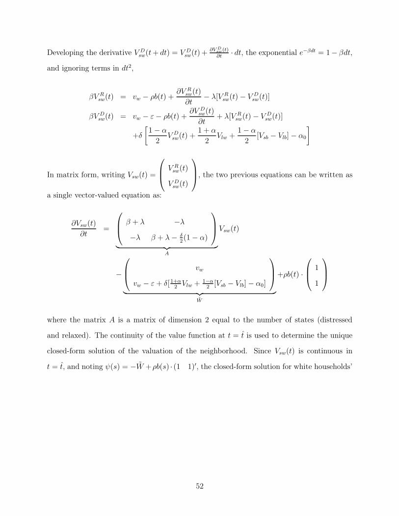
Developing the derivative V Dsw(t+ dt) = V D

sw(t) +∂V D

sw(t)∂t

· dt, the exponential e−βdt = 1− βdt,

and ignoring terms in dt2,

βV Rsw(t) = vw − ρb(t) +

∂V Rsw(t)

∂t− λ[V R

sw(t)− V Dsw(t)]

βV Dsw(t) = vw − ε− ρb(t) +

∂V Dsw(t)

∂t+ λ[V R

sw(t)− V Dsw(t)]

+δ

[1− α

2V Dsw(t) +

1 + α

2Vlw +

1− α

2[Vsb − Vlb]− α0

]

In matrix form, writing Vsw(t) =

V Rsw(t)

V Dsw(t)

, the two previous equations can be written as

a single vector-valued equation as:

∂Vsw(t)

∂t=

β + λ −λ

−λ β + λ− δ2(1− α)

︸ ︷︷ ︸

A

Vsw(t)

−

vw

vw − ε+ δ[1+α2Vlw + 1−α

2[Vsb − Vlb]− α0]

︸ ︷︷ ︸

W

+ρb(t) ·

1

1

where the matrix A is a matrix of dimension 2 equal to the number of states (distressed

and relaxed). The continuity of the value function at t = t is used to determine the unique

closed-form solution of the valuation of the neighborhood. Since Vsw(t) is continuous in

t = t, and noting ψ(s) = −W +ρb(s) · (1 1)′, the closed-form solution for white households’

52

valuation of the neighborhood for t ≤ t is, assuming the continuity of the value function.

Vsw(t) = eA(t−t)Vsw(t)−

ˆ t

t

e−A(s−t) · ψ(s)ds

= eA(t−t)Vsw(t) +

ˆ t

t

e−A(s−t) ·

W − ρb(s) ·

1

1

ds

= eA(t−t)Vsw(t) +A−1

t− t[1− exp(−A(t− t))] · W − ρ

ˆ t

t

e−A(s−t) ·

b(s)

b(s)

ds

where exp(−A(t − t)) is the exponential of the matrix −A(t − t), defined as exp X =∑

∞

k=01k!Xk. The value functions are decreasing with time as the fraction of blacks in the

neighborhood increases. Also the value functions are linear and decreasing in ρ.

Lemma 3. (Neighborhood composition at time t in racial transition) The number

of depressed and relaxed households, respectively D(t) and R(t), evolves in the following way.

• Before the tipping point, for t ≤ t, i.e. for b ≤ b.

D(t+ dt)−D(t) = −λD(t)dt+ λR(t)dt− δD(t)dt

R(t+ dt)− R(t) = −λR(t)dt+ λD(t)dt

Hence, writing D(t+dt)−D(t) = dDdt

·dt, the fraction of black, distressed white, relaxed

white households at time t is the solution to:

d

dt

D(t)

R(t)

=

−λ− δ λ

λ −λ

D(t)

R(t)

53

• After the tipping point, for t ≥ t, i.e. for b ≥ b = b(t),

D(t+ dt)−D(t) = −λD(t)dt+ λR(t)dt− δD(t)dt

R(t+ dt)− R(t) = −λR(t)dt+ λD(t)dt− δR(t)dt

And the total number of whites declines at rate δ, i.e. D(t) +R(t) = e−δ(t−t)(1− b(t)).

Hence, after the tipping point, the fraction of black, distressed white, relaxed white

households at time t is the solution to:

d

dt

D(t)

R(t)

=

−λ− δ λ

λ −λ− δ

D(t)

R(t)

The details of the solution are provided below.

Proof. Note C(t) = (D(t) R(t))′, K =

−λ− δ λ

λ −λ− δ

and L =

−λ− δ λ

λ −λ

.

Before the tipping point has been reached, note that L is a real symmetric matrix, hence

diagonalizable by the spectral theorem (Courant & Hilbert 1989). There is an orthogonal

matrix D such that K = D′Diag(k1, k2)D. Then the solution to the dynamics of the

neighborhood is C(t)=(D(t) R(t))′ = D′

c1ek1t + c2e

k2t

c1ek1t + c2e

k2t

, with c1, c2 chosen so that

D(0) equals the initial fraction of distressed whites, and R(0) = 1−D(0).

After the tipping point has been reached, note that D(t) +R(t) and D(t)− R(t) satisfy

the following homogeneous first-order differential equations:

[D(t+ dt) +R(t+ dt)]− [D(t) +R(t)] = −δ [D(t) +R(t)]

[D(t+ dt)− R(t+ dt)]− [D(t)− R(t)] = −(2λ+ δ) [D(t)−R(t)]

Hence the closed form solution for R(t) = 12{[D(t) +R(t)]− [D(t)−R(t)]}, and also for

D(t) = 12{[D(t) +R(t)] + [D(t)− R(t)]}.

54

Racial preferences and the Profit of Racial Transition

Proposition 4. Profit is linear and decreasing for ρ ≥ ρ, where ρ is the minimum level of

racial preferences for which t = b = 0.

Proof. If racial preferences ρ are above the threshold ρ, then t = b = 0. Then the p.d.v. of

revenue at time t = 0 is Π =´ t=∞

t=02δ {D(t)κ(pDb(t)) +R(t)κ(pRb(t))} e

−rtdt. Equation (16)

together with equation (17) show that the value functions V Rsw(t) and V D

sw(t) are decreasing

linear functions of ρ. Hence the prices pDb(t) and pRb(t) are linear decreasing functions of ρ

and the p.d.v. of revenues Π is a linear decreasing function of ρ for ρ ≥ ρ.

The Broker’s Discount Rate and the Profit of Racial Transition

Proposition 5. If the tipping point is b > 0, then there are two values r > 0 and r > 0 of

the time discount factor such that: when r /∈ [r; r], the p.d.v of revenue Π =´

∞

0π(t)e−rtdt

when steering to black is smaller than the p.d.v of revenues when steering to whites πss/r.

If the tipping point is b = 0, then an impatient broker has higher revenue when steering

to black than when steering to white. Formally, there is a finite r such that the p.d.v of

revenues´

∞

0π(t)e−rtdt when steering to black is larger than the p.d.v of revenues when

steering to whites for r > r, and smaller if r < r.

Proof. First, for r → 0 (an infinitely patient broker), the sign of´

∞

0π(t)e−rtdt−πss/r is the

sign of limt→∞ π(t) − πss, the difference between the revenues in an all-black neighborhood

and the revenues in a steady-state white neighborhood. This is negative. Hence, there exists

r > 0 such that r < r implies that the p.d.v. of revenues in a neighborhood in racial

transition is lower than the p.d.v of revenues in the steady-state white neighborhood.

Second, for r → ∞ (an infinitely impatient broker), the sign of´

∞

0π(t)e−rtdt− πss/r is

the sign of π(0)− πss. If the tipping point is nonzero, π(0) < πss, the broker makes initially

a lower revenue in the neighborhood in racial transition than in the all-white neighborhood.

Hence the existence of r > 0 that satisfies the conditions of the proposition.

55

Third, if the tipping point is zero, π(0) > πss, and for r → ∞, the p.d.v. of revenue

when steering to black is higher than the p.d.v. of revenue when steering to white. Also if

π(0) > πss, then π(t) is a decreasing function of time, hence´

∞

0π(t)e−rtdt is an increasing

function of r. Hence the existence of a unique r such that: the revenue of steering to black´

∞

0π(t)e−rtdt is larger than the steady-state all-white p.d.v. of revenues πss/r if and only if

r > r.

Black Households’ Outside Option and the Profit of Racial Transition

Proposition 6. Transaction prices are a decreasing function of black households’ outside

option. Formally, dpDb(t)/dVlb < 0 and dpRb(t)/dVlb < 0. The tipping point is an increasing

function of black households’ outside option. Formally, db/dVsb > 0 and dt/dVsb > 0. The

revenue of matching white sellers to black buyers is a decreasing function of blacks’ valuation

of housing outside the neighborhood. There is a value Vlb such that: steering white sellers to

black buyers leads to higher revenue than matching white sellers to white buyers for Vlb < Vlb.

Proof. First, we notice that the tipping point is an increasing function of Vlb. In equation

18, the valuation of the neighborhood (left-hand side of the equation) declines by δ(1 −

α)/2/(β + (1 + α)δ/2) when Vlb increases by 1, and the right hand side declines by 1 when

Vlb increases by 1. Since δ(1− α)/2/(β + (1+ α)δ/2) < 1, the tipping point is an increasing

function of black households’ outside option.

Second, transaction prices are a decreasing function of blacks’ outside option. Indeed,

pRb =12[(V R

sw(t)−Vlw)+(Vsb−Vlb)] and V Rsw(t) = V+e−δ(t−t) ρ(1−b(t))

(3+α) δ2+β

, with V =[δ[Vlw + 1−α

2[−Vlw + (Vsb − V

All terms are decreasing functions of Vlb.

Combining the first (increasing tipping point) and the second property (decreasing prices),

the broker’s revenue is a decreasing function of black buyers’ valuation of the outside option

Vsb.

56

Extension: Two Brokers

Proposition 7. In an equilibrium with two brokers either (i) no broker matches sellers to

blacks, and both brokers match to black t1 = t2 = ∞ or (ii) one broker, say broker 1, starts

matching sellers to blacks at t = 0, i.e. t1 = 0. The other broker, say broker 2, matches white

sellers to white buyers as long as the commission fees are larger when matching to whites,

hence t2 is the earliest point in time where π2,w(t2) = π2,b(t2) and where π2,w(t) ≥ π2,b(t) for

t ≤ t2.

Proof. Solving broker 2’s optimization program, we find that:

Π2(t) = π2,w(t)dt+ e−rdtΠ2(t+ dt) for t ≤ t2

Π2,b(t) = π2,b(t)dt+ e−rdtΠ2,b(t + dt) for t > t2

Hence, developing Π2(t+ dt) = Π2(t)+∂Π2

∂t(t)dt, e−rdt = 1− rdt and neglecting terms in dt2,

rΠ2(t) =∂Π2(t)

∂t+ π2,w(t) for t ≤ t2

rΠ2,b(t) =∂Π2,b(t)

∂t+ π2,b(t) for t > t2

The second equation is valid from t to ∞, and we know that (i) no trade takes place between

black sellers and any kind of buyer and that (ii) the neighborhood is entirely black for t→ ∞.

Hence π2,b(∞) = 0 and:

Π2,b(t) =

ˆ

∞

t

π2,b(s)e−rsds

The present discounted value of matching to blacks is equal to the present discounted value

of future revenues. By definition of the equilibrium, broker 2 matches sellers to white buyers

from t = 0 to t2. Hence,

Π2(t) = Π2,b(t2)er(t−t2) +

ˆ t2

t

π2,w(s)e−r(s−t)ds

57

t2 satisfies the following property: for t = 0 to t = t2, Π2(t) ≥ Π2,b(t) and Π2(t2) = Π2,b(t2).

That implies:ˆ t2

t

π2,w(s)e−r(s−t)ds ≥

ˆ t2

t

π2,b(s)e−r(s−t)ds

for all t ∈ [0, t2]. This therefore implies that πw(t) ≥ πb(t) for t ≤ t2 and πw(t2) = πb(t2).

Numerical Simulations for Figures 1 to 6

Parameters were set as follows: β = 6%, ρ = $1, 150 · β, vw = $9, 000, r = 5%, ε = $120,

Vsb = $10, 000, Vlb = $7, 800, Vlw = $6, 000, α = 6%, λ = 50%, δ = 1%.

58