Block 3 -Materials and Elasticity Lecture M17: Engineering Elastic Constants

There are three purposes to this block of lectures: 1. To complete our quick journey through continuum mechanics, to provide you with a

continuum version of a constitutive law - at least for linear elastic materials s pq = E ?emn

Elasticity Where does it come from?

2. Increasingly, materials are designed along with the structure, you need insight intowhat contributes to material properties. What you can control. What you cannot. This

will also allow us to understand the limits of the model of linear elasticity for a material.

3. To allow you to select quantitatively materials for applications as part of the design

process.

The lectures associated with objectives 2 and 3 will closely follow Ashby and Jones

chapters 1-7. This is an excellent reference and will not be supplemented by web-posted notes. The notes for the lectures associated with objective 1 are reproduced here.

Engineering Elastic Properties of Materials In order to understand how we link stress and strain we need to understand that there are

two points of view to this matter. There is the experimental point of view that some properties (behaviors) are easier to measure than others, and there is the mathematical

point of view that some representations of physical phenomena are mathematically easier to handle than others. In the present case, engineering elastic constants are derived from

an experimental point of view, whereas the stress and strain tensors, are mathematically

useful. Ultimately we need to resolve these two points of view.

†

†

†

Young’s modulus and Poisson’s ratio From the truss and strain laboratories you are now familiar with at least two elastic constants.

If we apply a uniaxial tensile stress s L to a constant cross-section rod of material, we

will obtain a biaxial state of strain, consisting of an axial tensile strain eL and a

transverse strain eT . The axial strain will be tensile for a tensile applied stress, and the

transverse strain will usually be compressive. We can measure the strains using resistance strain gauges.

†

†

†

For many materials, over some range of applied stress, the applied stress and the resulting

strains will follow a linear relationship. This observation is the basis for the definition of the engineering elastic constants. The Young’s modulus, E, is defined as the constant of

proportionality between a uniaxial applied stress and the resulting axial strain, i.e:

s L = EeL

Note. This only applies for a uniaxial applied stress, and the component of strain in the direction of the applied stress.

We can also define the Poisson’s ratio, n , as the ratio of the transverse strain to the axial strain. Since for the vast majority of materials the transverse strain is compressive for a

tensile applied stress, the Poisson’s ratio is defined as the negative of this ratio, to give a positive quantity. I.e:

eTn = -eL

A similar process, of performing experiments in which a well-defined stress state is applied and the resulting strain state is characterized leads us to define two other elastic

constants.

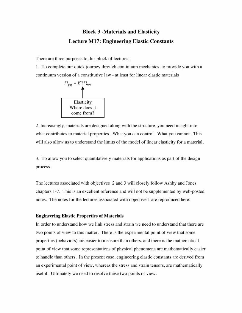
The Shear Modulus Application of a state of pure shear, leads to a shear strain:

Note angles are exaggerated in the figure.

†

†

†

†

An applied shear stress leads to an applied shear strain. The shear strain, g , is defined in

engineering notation, and therefore equals the total change in angle: g = q .

Consistent with the definition of the Young’s modulus, the Shear modulus. G, is defined as:

t = Gg

Again, note, that this relationship only holds if a pure shear is applied to a specimen.

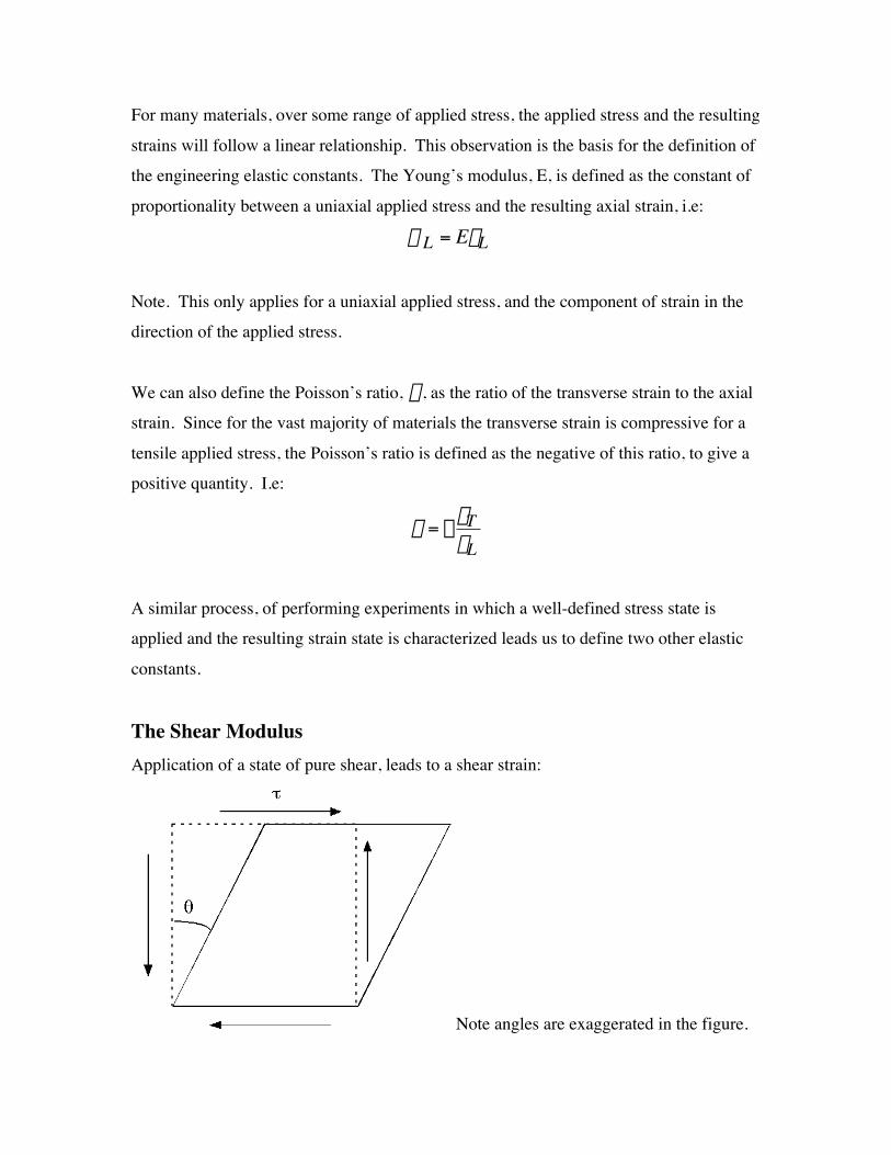
The Bulk Modulus The final elastic constant that is of interest to us is that of the bulk modulus. Materials

are slightly compressible. If a hydrostatic pressure, p, is applied to a volume of material, V, this will result in a slight reduction in volume, DV.

DVThis leads to a definition of the volumetric strain, D: D =

V

†

††

Thus we can define a bulk modulus, K, as: p = KD

Note, that if the pressure is represented as a stress, it would be negative, as would the change in volume.

For reasons that will become apparent later, The Young’s modulus, Shear Modulus, Bulk modulus and Poisson’s ratio are linked. For most materials Poission’s ratio’s are

3approximately 0.33, and for these materials K ª E and G ª E . However, values of

8 the Young’s modulus can vary widely.

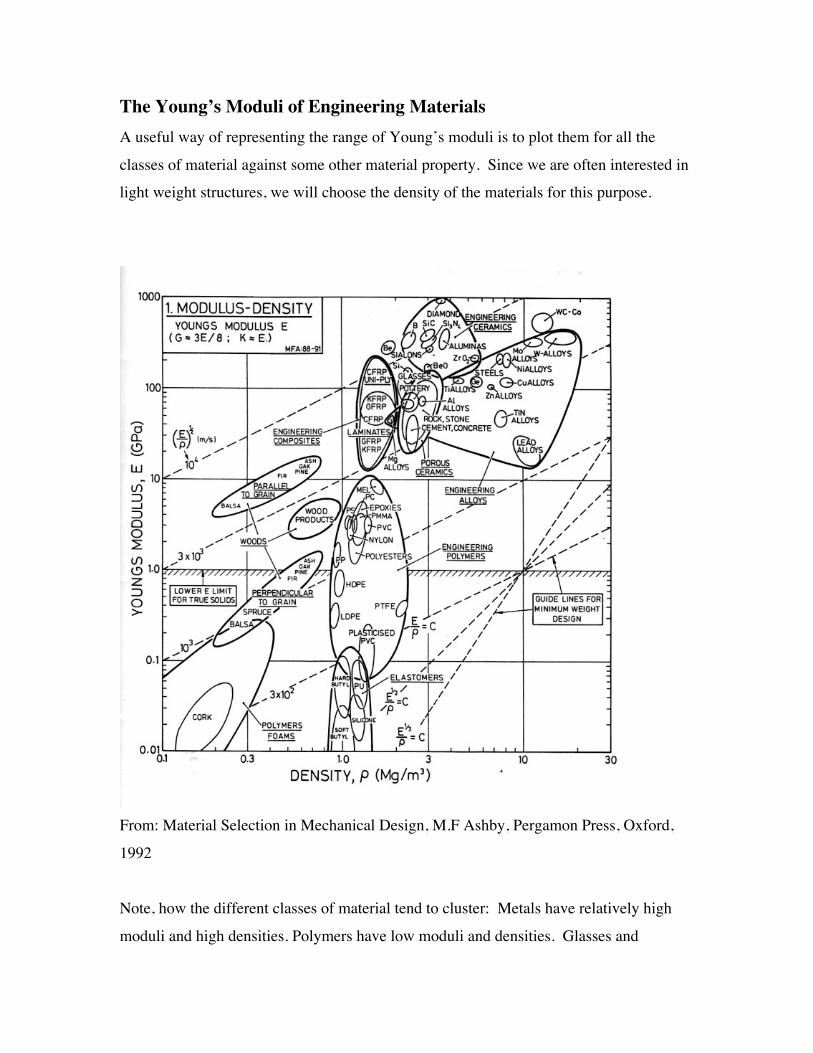
The Young’s Moduli of Engineering Materials A useful way of representing the range of Young’s moduli is to plot them for all the

classes of material against some other material property. Since we are often interested in light weight structures, we will choose the density of the materials for this purpose.

From: Material Selection in Mechanical Design, M.F Ashby, Pergamon Press, Oxford,

Note, how the different classes of material tend to cluster: Metals have relatively high

moduli and high densities. Polymers have low moduli and densities. Glasses and

1992

ceramics have high moduli and somewhat lower densities than metals. There are also

some materials that have quite wide ranges of moduli (and densities), while others (metals and ceramics) are relatively narrowly banded. Finally note how wide an overall

range of moduli is represented, from 0.01 GPA for foams to 1000 GPA for diamond. The range of densities is somewhat less, but still spans more than two orders of magnitude.

M18 Elastic moduli of composites, anisotropic materials We will return to better understand what leads to the moduli characteristic of different

classes of material in a few lectures time.

Now let’s get back to examining the elastic constants. Let us look more closely at one

particular class of material, fiber composites. Reference to the material property chart above we can see that composites (CFRP – carbon fiber reinforced polymers) have higher

modulus to density ratio’s than many metals. Why is this?

The key is that very fine (6 µm diameter) carbon fibers can be produced with a modulus

comparable to that of ceramics (200-1000 GPa). These fibers also have very tensile high strengths, much higher than normally exhibited by bulk ceramics, which tend to be

brittle, and have a low strength as a result. However, they are fibers, so they cannot carry multiaxial loads on their own. However, if they are surrounded by a “matrix” to provide

lateral support, and to transfer load between fibers if one fiber happens to break, they can

result in materials with high moduli and strengths. Polymers such as epoxy resins are often used as matrices.

E

Let us examine how we can estimate the Young’s modulus of the resulting composite

material. Initially we will consider a two dimensional case. 2-D fibers interspersed with

a 2-D matrix. The fibers have a Young’s modulus Ef and the matrix a Young’s modulus

m

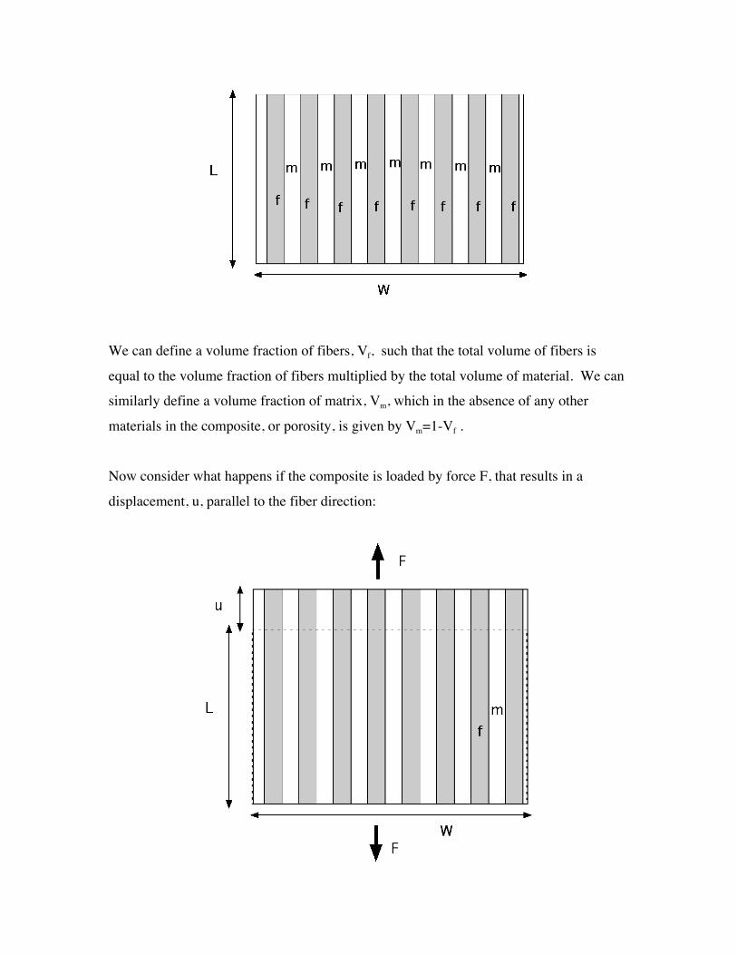
We can define a volume fraction of fibers, Vf, such that the total volume of fibers is

equal to the volume fraction of fibers multiplied by the total volume of material. We can similarly define a volume fraction of matrix, Vm, which in the absence of any other

materials in the composite, or porosity, is given by Vm=1-Vf .

Now consider what happens if the composite is loaded by force F, that results in a

displacement, u, parallel to the fiber direction:

†

† †

†

†

†

†

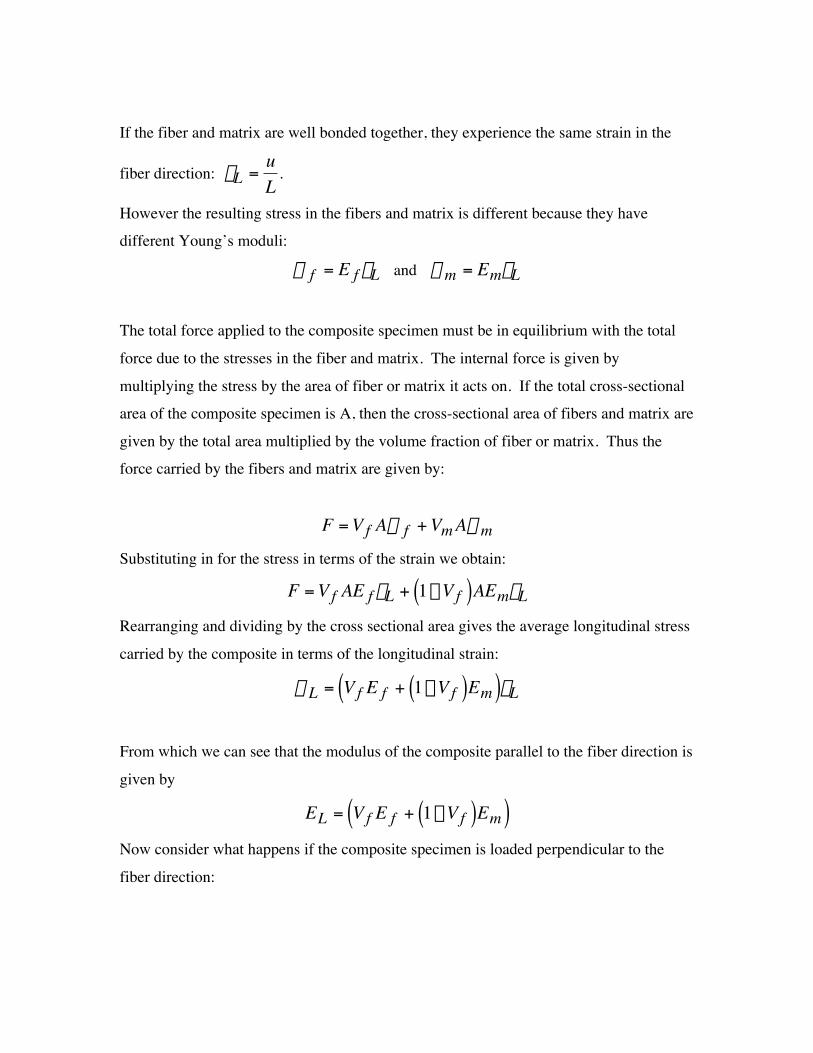
If the fiber and matrix are well bonded together, they experience the same strain in the

ufiber direction: eL = .

L However the resulting stress in the fibers and matrix is different because they have different Young’s moduli:

s f = E f eL and s m = EmeL

The total force applied to the composite specimen must be in equilibrium with the total

force due to the stresses in the fiber and matrix. The internal force is given by

multiplying the stress by the area of fiber or matrix it acts on. If the total cross-sectional area of the composite specimen is A, then the cross-sectional area of fibers and matrix are

given by the total area multiplied by the volume fraction of fiber or matrix. Thus the force carried by the fibers and matrix are given by:

F = V f As f + Vm As m

Substituting in for the stress in terms of the strain we obtain:

F = V f AE f eL + (1 - V f )AEmeL

Rearranging and dividing by the cross sectional area gives the average longitudinal stress

carried by the composite in terms of the longitudinal strain:

s L = (V f E f + (1 - V f )Em )eL

From which we can see that the modulus of the composite parallel to the fiber direction is

given by

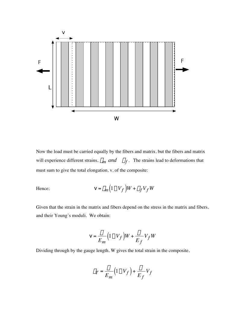
EL = (V f E f + (1 - V f )Em ) Now consider what happens if the composite specimen is loaded perpendicular to the

fiber direction:

†

†

†

†

Now the load must be carried equally by the fibers and matrix, but the fibers and matrix

will experience different strains, em and e f . The strains lead to deformations that

must sum to give the total elongation, v, of the composite:

Hence; v = em (1 - V f )W + e f V f W

Given that the strain in the matrix and fibers depend on the stress in the matrix and fibers,

and their Young’s moduli. We obtain:

s v = (1 - V f )W + E s

f V f W

Em

Dividing through by the gauge length, W gives the total strain in the composite,

s eT = (1 - V f ) +

E s

f V fEm

†

From which we can see that the Young’s modulus of the composite transverse to the fiber

direction is given by:

1ET = (1 - V f )

+ V f

Em E f

Which is different from the Young’s modulus parallel to the fiber direction. Thus fiber

composites are an example of a material that has different properties in different

directions. This is termed “anisotropy” and most fiber composites are “anisotropic”. Materials which have the same properties in all directions are termed “isotropic”.

Note, that the estimate for the Young’s modulus of a fiber composite parallel to the fiber

direction is very good, however, the estimate for the Young’s modulus perpendicular to

the fiber direction underestimates the value you would measure experimentally.

Since we are interested in composite materials for many structural applications, we would like to have a method for linking general stress and strain that can account for anisotropy.

So back to continuum elasticity.

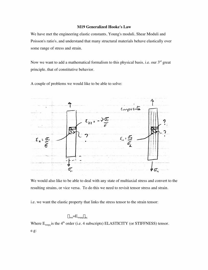
M19 Generalized Hooke's Law We have met the engineering elastic constants, Young's moduli, Shear Moduli and Poisson's ratio's, and understand that many structural materials behave elastically over

some range of stress and strain.

Now we want to add a mathematical formalism to this physical basis, i.e. our 3rd great

principle, that of constitutive behavior.

A couple of problems we would like to be able to solve:

We would also like to be able to deal with any state of multiaxial stress and convert to the

resulting strains, or vice versa. To do this we need to revisit tensor stress and strain.

i.e. we want the elastic property that links the stress tensor to the strain tensor:

esmn=Emnpq pq

Where E is the 4th order (i.e. 4 subscripts) ELASTICITY (or STIFFNESS) tensor.mnpq

e.g:

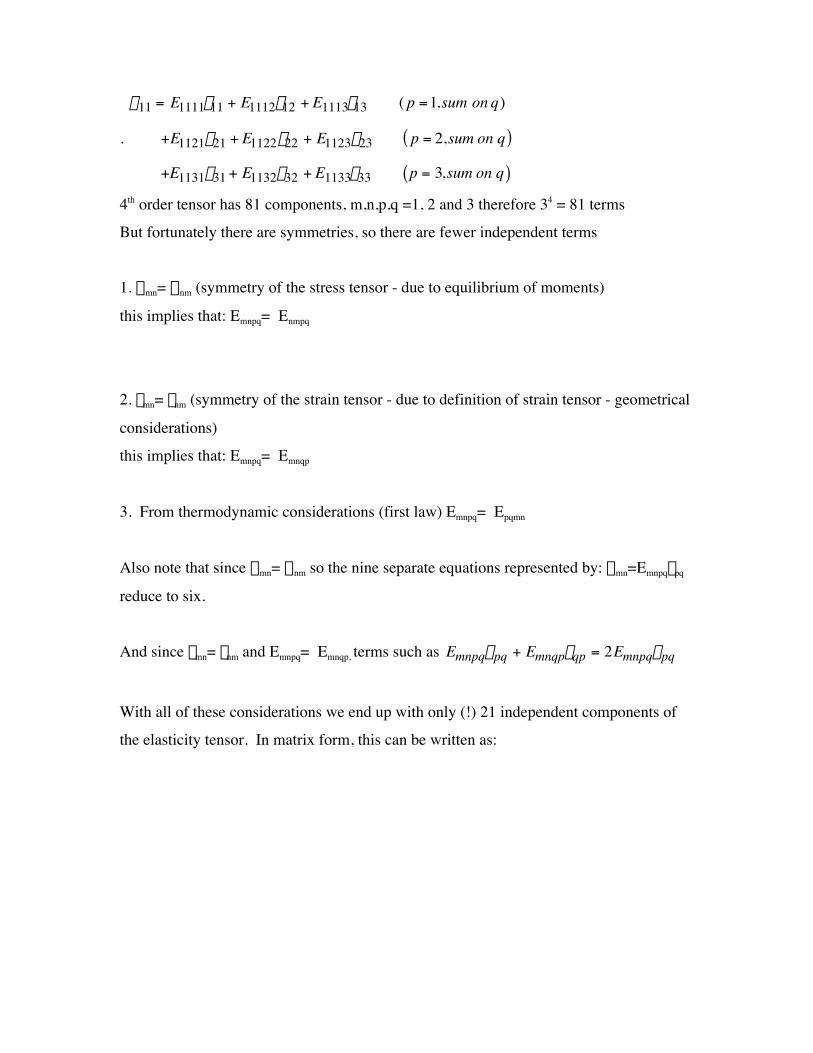
s11 = E1111e11 + E1112e12 + E1113e13 ( p = 1,sum on q )

. +E1121e21 + E1122e22 + E1123e23 ( p = 2, sum on q )

+E1131e31 + E1132e32 + E1133e33 (p = 3,sum on q )

4th order tensor has 81 components, m,n,p,q =1, 2 and 3 therefore 34 = 81 terms

But fortunately there are symmetries, so there are fewer independent terms

1. smn= snm (symmetry of the stress tensor - due to equilibrium of moments)

this implies that: Emnpq= Enmpq

2. emn= enm (symmetry of the strain tensor - due to definition of strain tensor - geometrical

considerations)

this implies that: Emnpq= Emnqp

3. From thermodynamic considerations (first law) Emnpq= Epqmn

Also note that since smn= snm so the nine separate equations represented by: smn=E emnpq pq

reduce to six.

And since emn= enm and Emnpq= E terms such as Emnpqe pq + Emnqpeqp = 2Emnpqe pqmnqp,

With all of these considerations we end up with only (!) 21 independent components of

the elasticity tensor. In matrix form, this can be written as:

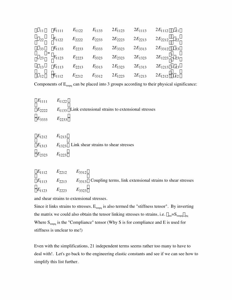
Ïs11 ̧ È E1111 E1122 E1133 2E1123 2E1113 2 E1112 ̆ Ïe11 ̧ Ô Ô Í Ô Ô

s22 E1122 E2222 E2233 2E2223 2E2213 2 E2212 ˙Ô e22

ÔÔ Í ˙Ô Ôs33 Ô Í E1133 E2233 E3333 2E3323 2E3313 2 E3312 ̇ Ôe33 Ô Ì ˝ = Í Ì ˝ Ôs23 Ô Í

E1123 E2223 E3323 2E2323 2E1323 2E1223 ˙ Ôe23 Ô˙

ÔÔs13 Ô Í E1113 E2213 E3313 2E1323 2E1313 2E1213 ̇ Ôe13 Ô Ô Í Ô Ô Ós12 ̨ ÎE1112 E2212 E3312 2E1223 2E1213 2 E1212 ̊

˙Óe12 ̨

Components of Emnpq can be placed into 3 groups according to their physical significance:

¸Ï E1111 E1122Ô Ô

˝ Link extensional strains to extensional stressesÌ E2222 E1133 Ô ÔÓ E3333 E2233 ̨

¸Ï E1212 E1213Ô Ô

Link shear strains to shear stressesÌ E1313 E1323 ̋ Ô ÔÓ E2323 E1223 ̨

¸Ï E1112 E2212 E3312Ô Ô Ì E1113 E2213 E3313 ̋ Coupling terms, link extensional strains to shear stresses Ô ÔÓ E1123 E2223 E3323 ̨

and shear strains to extensional stresses. Since it links strains to stresses, Emnpq is also termed the "stiffness tensor". By inverting

the matrix we could also obtain the tensor linking stresses to strains, i.e. emn=S smnpq pq

Where Smnpq is the "Compliance" tensor (Why S is for compliance and E is used for stiffness is unclear to me!)

Even with the simplifications, 21 independent terms seems rather too many to have to deal with!. Let's go back to the engineering elastic constants and see if we can see how to

simplify this list further.

_ _ _ _ _ _

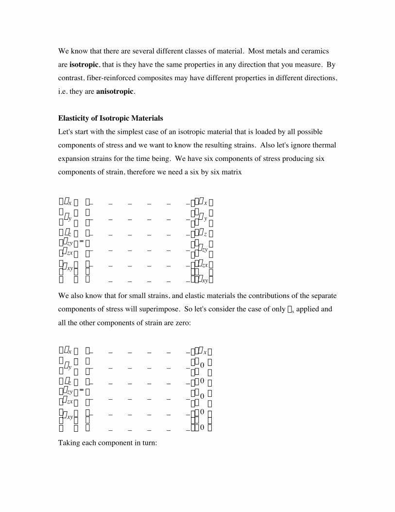
We know that there are several different classes of material. Most metals and ceramics

are isotropic, that is they have the same properties in any direction that you measure. By contrast, fiber-reinforced composites may have different properties in different directions,

i.e. they are anisotropic.

Elasticity of Isotropic Materials Let's start with the simplest case of an isotropic material that is loaded by all possible components of stress and we want to know the resulting strains. Also let's ignore thermal

expansion strains for the time being. We have six components of stress producing six components of strain, therefore we need a six by six matrix

e xÊ ˆ _Ê _ _ _ _ _ˆ s xÊ ˆ

e y Á Á

˜ ˜

_ Á Á

_ _ _ _ _ ̃ ˜

s y Á Á

˜ ˜

ezÁ ˜ _Á _ _ _ _ _˜ s zÁ ˜ g zy g zx

Á Á

˜ ˜

= _ Á

Á _ _ _ _ _ ̃

˜ t zy

Á Á

˜ ˜

g xy Á Á

˜ ˜

_Á Á

_ _ _ _ _˜ ˜

t zxÁ Á

˜ ˜

Ë ¯ Ë _ _ _ _ _¯ t xyË ¯

We also know that for small strains, and elastic materials the contributions of the separate components of stress will superimpose. So let's consider the case of only sx applied and

all the other components of strain are zero:

Ê e x ˆ Ê _ _ _ _ _ _ˆ Ês x ̂ Á

e y ˜ Á _ _ _ _ _ _ ̃ Á 0 ˜

Á ˜ Á ˜ Á ˜ Á ez ˜ Á _ _ _ _ _ _˜ Á 0 ˜

=Ág zy ̃ Á ˜ Á 0 ˜ Ág zx ̃ Á ˜ Á ˜

Á _ _ _ _ _ _˜ Á 0 ˜Ág xy ̃ ˜

ÁÁ ˜ Á ˜ Ë ¯ Ë _ _ _ _ _¯ Ë 0 ¯

Taking each component in turn:

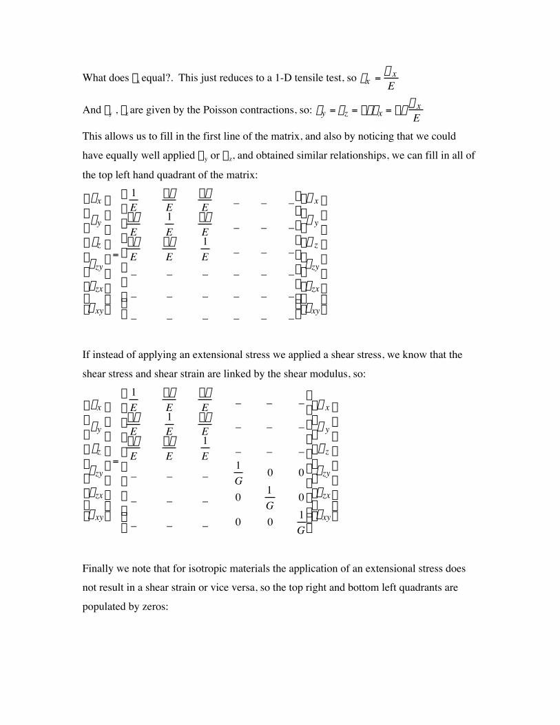
What does ex equal?. This just reduces to a 1-D tensile test, so ex =s x E

And ey , ez are given by the Poisson contractions, so: ey = e z = -ne x = -ns x E

This allows us to fill in the first line of the matrix, and also by noticing that we could

have equally well applied s or sz, and obtained similar relationships, we can fill in all ofy

the top left hand quadrant of the matrix: -n -nÊ e x ˆ

Ê 1 _ _ _ ̂ Ê s x ˆE E ˜ Á ˜Á ˜ Á Á

-E n 1 -n _ _ _˜ Á

s y ˜

e yÁ ˜ Á E E E

Á ez ˜ -n -n 1 ˜ Á s z ˜ _ _ _˜ Á ˜Á ˜ =Á E E E

tÁ g zy Á _ zy

˜ _ _ _ _ _ ̃ Á ˜ Á g zx ̃

Á ˜ Át zx ̃ _ _ _ _ _ _˜ Á ˜Á ˜ ÁÁ

Ëg xy ̄ _ ̄ ˜ Ët xy ̄Ë _ _ _ _ _

If instead of applying an extensional stress we applied a shear stress, we know that the

shear stress and shear strain are linked by the shear modulus, so:

Ê 1 -n -n ˆ _ _ _ ˜ Ê s x ˆÊ e x ˆ Á E E E

Á ˜ Á -n 1 -n _ _ _ ̃ Á s ˜e y yÁ E E Á ˜˜ Á -

E n -n 1 ˜

_ _ _ ̃Á ez ˜ Á E Á sz ˜E E=Á ˜ Á 1 tÁ g zy _ _ _ 0 0 ̃

Á Á

zy ˜

˜ Á G ˜ ˜ Á g zx ̃ Á _ _ _ 0 1 0 ̃ Á

Á t zx ̃

Á Ëg xy ̄

˜ ÁÁ

G ˜˜

Ë _ _ _ 0 0 1 ̃ Ët xy ̄ G ̄

Finally we note that for isotropic materials the application of an extensional stress does not result in a shear strain or vice versa, so the top right and bottom left quadrants are

populated by zeros:

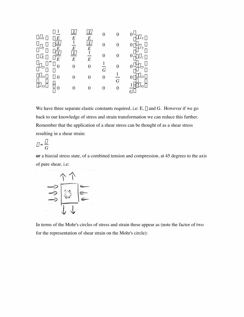
Ê 1 -n -n 0 0 0 ̂ Ê e x ˆ Á E E E ˜ Ê s x ˆ Á ˜ Á -n 1 -n 0 0 0 ̃ Á

s ˜e y yÁ E E Á ˜˜ Á -E n -n 1 ˜

Á ez ˜ Á E 0 0 0 ̃ Á sz ˜E E=Á ˜ Á 1 t

Á g zy 0 0 0 0 0 ̃

Á Á

zy ˜

˜ Á G ˜ ˜ Á g zx ̃ Á 0 0 0 0 1 0 ̃ Át zx ̃ Á Ëg xy ̄

˜ ÁÁ

G Á ˜˜

Ë 0 0 0 0 0 1 ̃ Ët xy ̄ G ̄

We have three separate elastic constants required, i.e: E, n and G. However if we go

back to our knowledge of stress and strain transformation we can reduce this further. Remember that the application of a shear stress can be thought of as a shear stress

resulting in a shear strain: t

g = G

or a biaxial stress state, of a combined tension and compression, at 45 degrees to the axis

of pure shear, i.e:

In terms of the Mohr's circles of stress and strain these appear as (note the factor of two

for the representation of shear strain on the Mohr's circle):

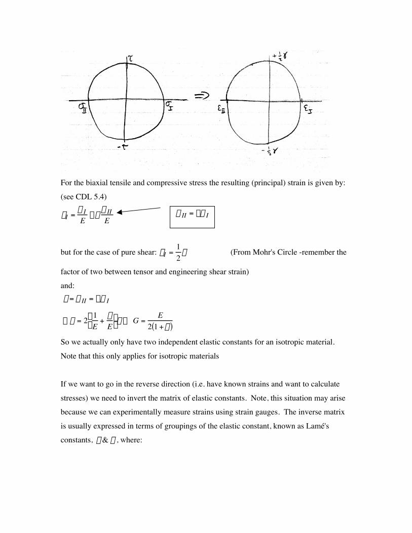
For the biaxial tensile and compressive stress the resulting (principal) strain is given by:

(see CDL 5.4) s I s II = -s IeI = -n s IIE E

1but for the case of pure shear: eI = 2

g (From Mohr's Circle -remember the

factor of two between tensor and engineering shear strain) and: t = s II = -s I

Ê 1 n ˆt fi G = E

¯ ( \g = 2Ë E

+ E 2 1 +n )

So we actually only have two independent elastic constants for an isotropic material.

Note that this only applies for isotropic materials

If we want to go in the reverse direction (i.e. have known strains and want to calculate

stresses) we need to invert the matrix of elastic constants. Note, this situation may arise because we can experimentally measure strains using strain gauges. The inverse matrix

is usually expressed in terms of groupings of the elastic constant, known as Lamé's constants, m & l , where:

- -

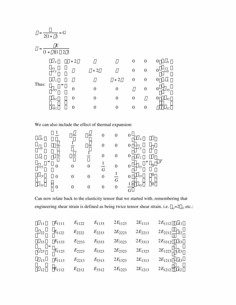
E m = = G

2 1+ n)(

nE l =

(1 +n )(1 - 2n)

Ês x ˆ Êl + 2m l l 0 0 0ˆ Ê e x ˆ Á ˜ Á ˜ Á ˜ Á

s y ˜ Á

l l + 2m l 0 0 0 e y˜ Á ˜

Á s z ̃ Á l l l + 2m 0 0 0˜ Á ez ˜ Thus: Á =

t xy ˜ Á 0 0 0 m 0 0

˜ ˜

Á Á g xy

˜ Á ˜ Á Át xz ̃ Á 0 0Á ˜ Á Ëtyz ̄ Ë 0 0

˜ 0 0 m 0˜ Ág xz ̃

˜ Á ˜ 0 0 0 m¯Ëg yz ̄

We can also include the effect of thermal expansion:

Ê 1 n n Ê e x ˆ Á E E E

0 0 0 ˆ ˜ Ês x ˆ Êaˆ

nÁ ˜ Á -n 1

- 0 0 0 ˜ Á s ˜ Á ˜e y yE E EÁ ˜ Á n n 1 ˜ Á ˜ Á

a˜

Á ez ˜ Á - E - 0 0 0 ˜ Ás z ˜ Áa˜E=Á ˜ Á 1 Á ˜

Ág zy 0 0

E

0 0 0 ˜ t zy ˜ + Á 0

DT

˜ Á G ˜ Á ˜ Á ˜ Á g zx ̃ Á 0 0 0 0 1 0 ˜ Át zx ̃ Á 0˜ Á Ëg xy ̄

˜ ÁÁ

G Á ˜ Á ˜ ˜

Ë 0 0 0 0 0 1 ˜ Ët xy ̄ Ë 0¯

G ̄

Can now relate back to the elasticity tensor that we started with, remembering that

engineering shear strain is defined as being twice tensor shear strain, i.e. gxy=2e12 etc.:

Ïs11 ̧ È E1111 E1122 E1133 2E1123 2E1113 2 E1112 ̆ Ïe11 ̧ Ô Ô Í Ô Ô

s22 E1122 E2222 E2233 2E2223 2E2213 2 E2212 ˙Ô e22

ÔÔ Í ˙Ô Ôs33 Ô Í E1133 E2233 E3333 2E3323 2E3313 2 E3312 ̇ Ôe33 Ô Ì ˝ = Í Ì ˝ Ôs23 Ô Í

E1123 E2223 E3323 2E2323 2E1323 2E1223 ˙ Ôe23 Ô˙

ÔÔs13 Ô Í E1113 E2213 E3313 2E1323 2E1313 2E1213 ̇ Ôe13 Ô Ô Í Ô Ô Ós12 ̨ ÎE1112 E2212 E3312 2E1223 2E1213 2 E1212 ̊

˙Óe12 ̨

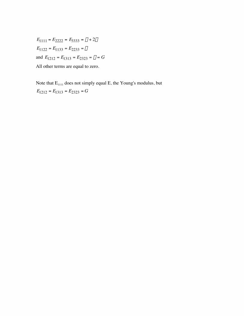
= l + 2mE1111 = E2222 = E3333

= lE1122 = E1133 = E2233

= m = Gand E1212 = E1313 = E2323

All other terms are equal to zero.

Note that E1111 does not simply equal E, the Young's modulus, but = GE1212 = E1313 = E2323

Elasticity for Non-Isotropic Materials

For more elastically complicated materials more of the elastic constants take on different

values according to the direction in which they are measured. This is known as anisotropy. We will consider two important cases of composites:

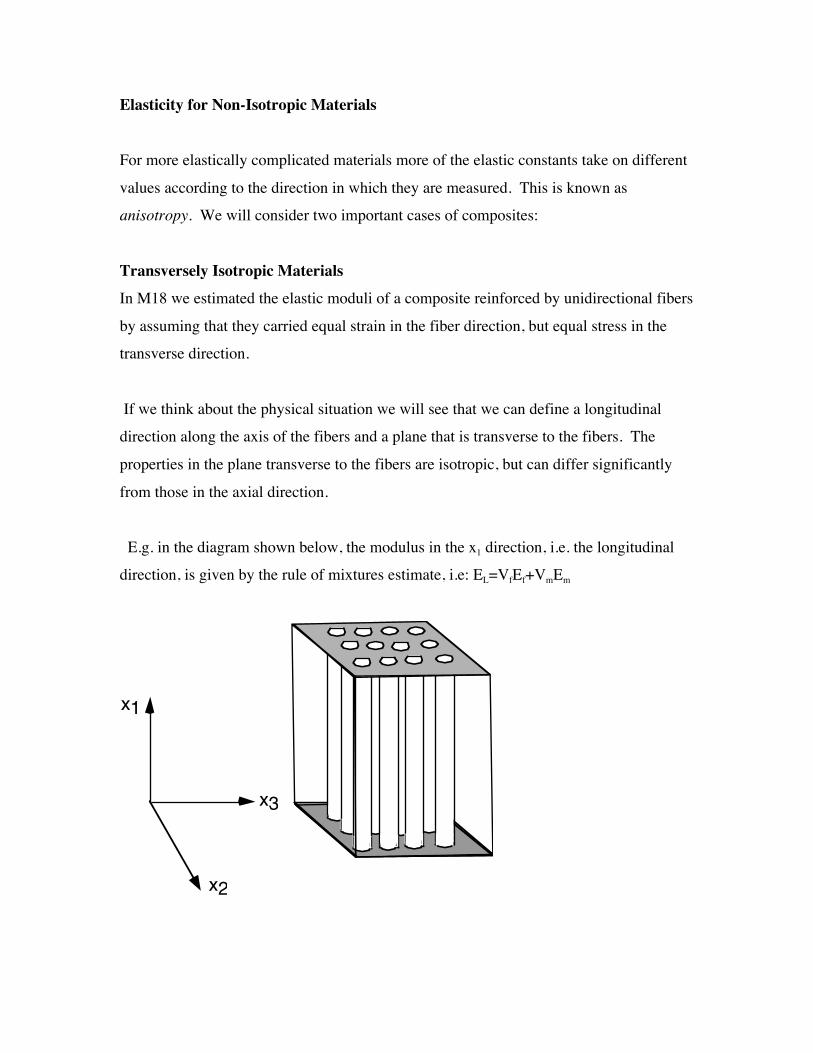
Transversely Isotropic Materials In M18 we estimated the elastic moduli of a composite reinforced by unidirectional fibers

by assuming that they carried equal strain in the fiber direction, but equal stress in the transverse direction.

If we think about the physical situation we will see that we can define a longitudinal direction along the axis of the fibers and a plane that is transverse to the fibers. The

properties in the plane transverse to the fibers are isotropic, but can differ significantly

from those in the axial direction.

E.g. in the diagram shown below, the modulus in the x1 direction, i.e. the longitudinal direction, is given by the rule of mixtures estimate, i.e: EL=VfEf+VmEm

x1

x2

x3

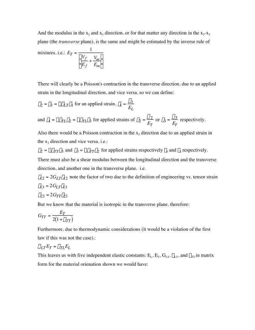
And the modulus in the x2 and x3 direction, or for that matter any direction in the x2-x3

plane (the transverse plane), is the same and might be estimated by the inverse rule of 1mixtures, i.e.: ET =

Ï Vf ¸VmÌ + ˝ Ó E f Em ̨

There will clearly be a Poisson's contraction in the transverse direction, due to an applied strain in the longitudinal direction, and vice versa, so we can define:

e2 = e3 = -nLTe1 for an applied strain, e1 =s1 EL

and e1 = -nTLe2 = -nTLe3 for applied strains of e2 =s 2 or e3 =

s3 respectively.ET ET

Also there would be a Poisson contraction in the x2 direction due to an applied strain in the x3 direction and vice versa, i.e.: e2 = -nTTe3 and e3 = -nTTe2 for applied strains respectively e3 and e2 respectively.

There must also be a shear modulus between the longitudinal direction and the transverse

direction, and another one in the transverse plane. i.e. t12 = 2GLTe12 note the factor of two due to the definition of engineering vs. tensor strain

t13 = 2GLTe13

t23 = 2GTTe23

But we know that the material is isotropic in the transverse plane, therefore: ET=GTT (2 1 +nTT )

Furthermore, due to thermodynamic considerations (it would be a violation of the first law if this was not the case).:

= nTLELn LT ET

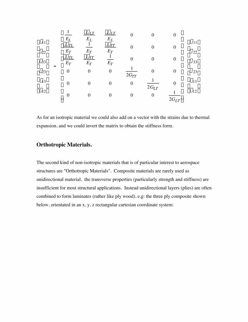
This leaves us with five independent elastic constants: EL, ET, GLT, nLT, and nTT in matrix

form for the material orienation shown we would have:

È 1 -n LT -n LT 0 0 0 ˘ Í EL EL EL ˙

Ïs11 ̧Ïe11 ̧ Í -nTL 1 -nTT 0 0 0 ˙

Ô ÔÔ Ô Ô e22 Í ET ET ET ˙

Ô s 22

Ô Ô--nTL nTTÔe33 Ô Í

ET E1 T

0 0 0 ˙ Ôs 33 Ô Ì ˝ = Í ET

1 ˙ Ì ˝ Ôe23 Ô Í 0 0 0 0 0 ˙ Ôs 23 Ô Ôe13 Ô Í

2GTT 1 0

˙ Ôs13 Ô 0 0 0 ˙ Ô ÔÔ Ô Í 0

Óe12 ̨ Í Í 0 0 0 Î

2GLT 1 ˙ Ós12 ̨

0 0 2GLT ˚̇

As for an isotropic material we could also add on a vector with the strains due to thermal expansion, and we could invert the matrix to obtain the stiffness form.

Orthotropic Materials.

The second kind of non-isotropic materials that is of particular interest to aerospace structures are "Orthotropic Materials". Composite materials are rarely used as

unidirectional material, the transverse properties (particularly strength and stiffness) are

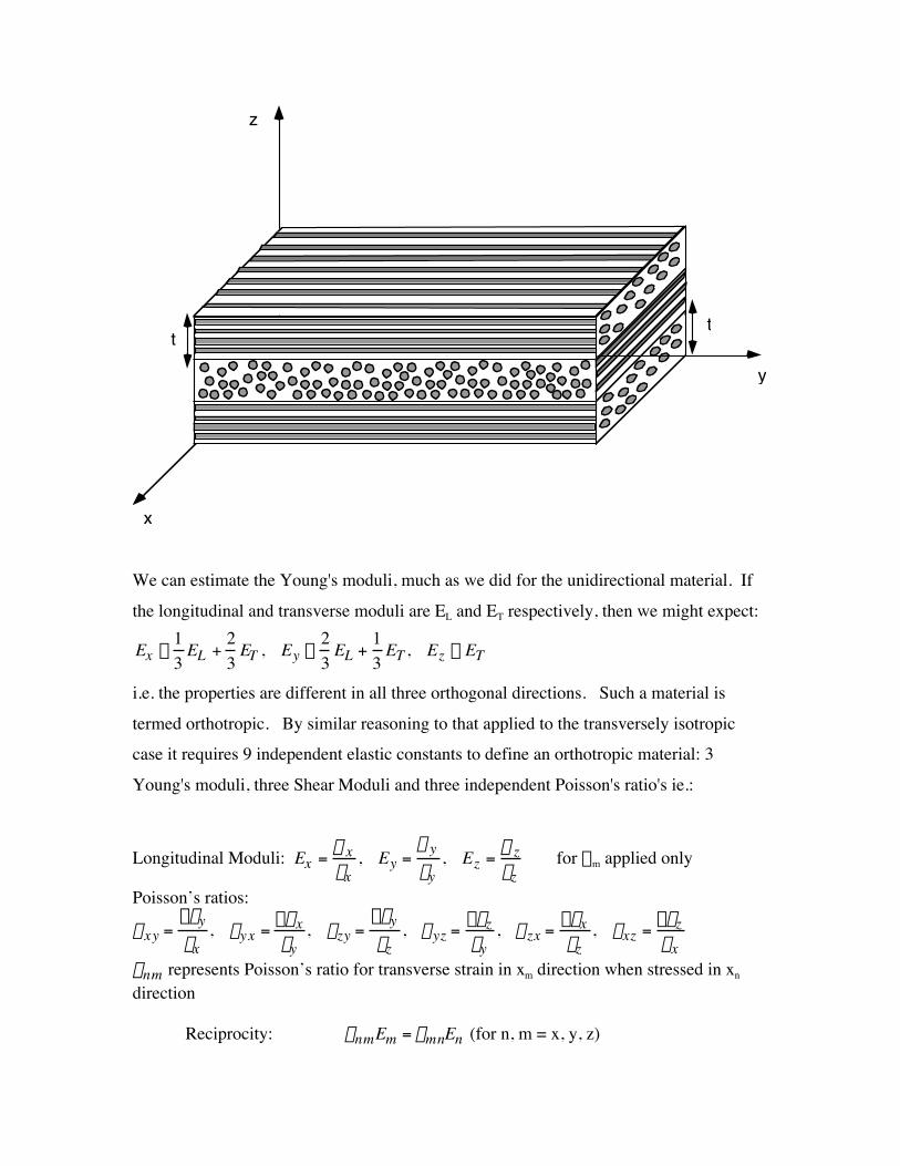
insufficient for most structural applications. Instead unidirectional layers (plies) are often combined to form laminates (rather like ply wood), e.g: the three ply composite shown

below, orientated in an x, y, z rectangular cartesian coordinate system:

y

z

t

x

t

We can estimate the Young's moduli, much as we did for the unidirectional material. If

the longitudinal and transverse moduli are EL and ET respectively, then we might expect:

Ex ª13

EL +23

ET , Ey ª23

EL +13

ET , Ez ª ET

i.e. the properties are different in all three orthogonal directions. Such a material is

termed orthotropic. By similar reasoning to that applied to the transversely isotropiccase it requires 9 independent elastic constants to define an orthotropic material: 3

Young's moduli, three Shear Moduli and three independent Poisson's ratio's ie.:

Longitudinal Moduli: Ex =s xex

, Ey =s yey

, Ez =s zez

for sm applied only

Poisson’s ratios:

n xy =-eyex

, nyx =-e xey

, nzy =-eyez

, n yz =-ezey

, n zx =-exez

, nxz =-eze x

nnm represents Poisson’s ratio for transverse strain in xm direction when stressed in xn

direction

Reciprocity: nnmEm = nmnEn (for n, m = x, y, z)

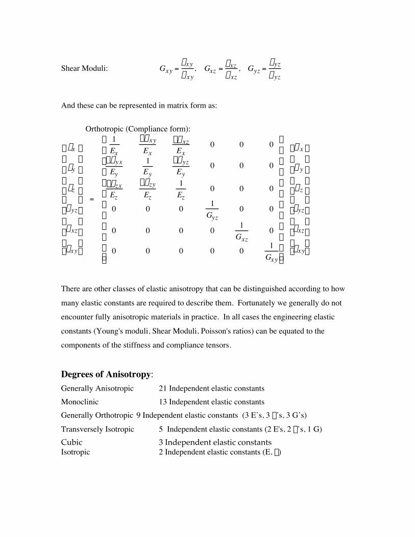
t yzShear Moduli: Gxy =t xy , Gxz =

t xz , G = g xy g xz

yz g yz

And these can be represented in matrix form as:

Orthotropic (Compliance form):

Ï ex ¸ È Í E

1 x

-n xy -n xz 0 0 0 ˙ ˘

Ïs x ¸Ex ExÔ Ô Í -nyx 1 -n yz ˙ Ô Ô Ô ey Ô Í E E E

0 0 0 ˙ Ôs y Ô y y

Ô Ô Í -nyzx -nzy 1 ˙ Ô Ô

ezÔ Ô Í Ez 0 0 0 Ôsz Ô˙

Ì ˝ = Ez Ez 1 Ì ˝

Í ˙Ôg yzÔ 0 0 0 0 0

˙ Ôt yzÔ

Í GyzÔ Ô Ô Ô1 ˙Ôg xzÔ

Í 0 0 0 0 0 Ôt xzÔ˙

Ô Ô Í Gxz Ô Ô

Óg xy˛ Í 0 0 0 0 0 1 ˙ Ót xy˛ÍÎ Gxy ̊̇

There are other classes of elastic anisotropy that can be distinguished according to how

many elastic constants are required to describe them. Fortunately we generally do notencounter fully anisotropic materials in practice. In all cases the engineering elastic

constants (Young's moduli, Shear Moduli, Poisson's ratios) can be equated to the

components of the stiffness and compliance tensors.

Degrees of Anisotropy:Generally Anisotropic 21 Independent elastic constants

Monoclinic 13 Independent elastic constants

Generally Orthotropic 9 Independent elastic constants (3 E’s, 3 n’s, 3 G’s)Transversely Isotropic 5 Independent elastic constants (2 E's, 2 n’s, 1 G)Cubic 3 Independent elastic constantsIsotropic 2 Independent elastic constants (E, n)