Block 2: Introduction to Information Theory · Block 2: Introduction to Information Theory ... 3 Source coding 4 Mutual information 5 Discrete channels 6 Entropy and mutual information

Block 2: Introduction to Information Theory

Francisco J. Escribano

April 26, 2015

Francisco J. Escribano Block 2: Introduction to Information Theory April 26, 2015 1 / 51

Table of contents

1 Motivation

2 Entropy

3 Source coding

4 Mutual information

5 Discrete channels

6 Entropy and mutual information for continuous RRVV

7 Channel capacity theorem

8 Conclusions

9 References


Motivation

Motivation


Motivation

Motivation

Information Theory is a discipline established during the 2nd half of theXXth Century.

It relies on solid mathematical foundations [1, 2, 3, 4].

It tries to address two basic questions:

◮ To what extent can we compress data for a more efficient usage of thelimited communication resources?

→ Entropy

◮ Which is the largest possible data transfer rate for given resources andconditions?

→ Channel capacity

Key concepts for Information Theory are entropy (H (X)) and mutualinformation (I (X; Y)).

◮ X, Y are random variables of some kind.


Motivation

Motivation

Up to the 40’s, it was common wisdom in telecommunications that theerror rate increased with increasing data rate.

◮ Claude Shannon demonstrated that errorfree transmission may be pos-sible under certain conditions.

Information Theory provides strict bounds for any communication sys-tem.

◮ Maximum data compression → minimum I(

X; X̂)

.

◮ Maximum data transfer rate → maximum I (X; Y).

Any given communication system works between said limits.

The mathematics behind is not always constructive, but provides guide-lines to design algorithms to improve communications given a set ofavailable resources.

◮ The resources in this context are known parameters such us available

transmission power, available bandwidth, signal-to-noise ratio andthe like.


Entropy

Entropy


Entropy

Entropy

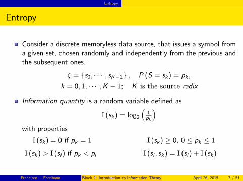
Consider a discrete memoryless data source, that issues a symbol froma given set, chosen randomly and independently from the previous andthe subsequent ones.

ζ = {s0, · · · , sK−1} , P (S = sk) = pk ,

k = 0, 1, · · · , K − 1; K is the source radix

Information quantity is a random variable defined as

I (sk) = log2

(

1pk

)

with properties

I (sk) = 0 if pk = 1

I (sk) > I (si) if pk < pi

I (sk) ≥ 0, 0 ≤ pk ≤ 1

I (sl , sk) = I (sl) + I (sk)


Entropy

Entropy

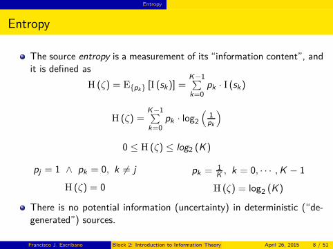
The source entropy is a measurement of its “information content”, andit is defined as

H (ζ) = E{pk } [I (sk)] =K−1∑

k=0pk · I (sk)

H (ζ) =K−1∑

k=0pk · log2

(

1pk

)

0 ≤ H (ζ) ≤ log2 (K )

pj = 1 ∧ pk = 0, k 6= j

H (ζ) = 0

pk = 1K , k = 0, · · · , K − 1

H (ζ) = log2 (K )

There is no potential information (uncertainty) in deterministic (“de-generated”) sources.


Entropy

Entropy

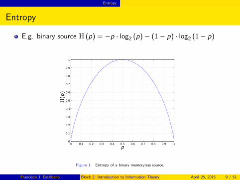
E.g. binary source H (p) = −p · log2 (p) − (1 − p) · log2 (1 − p)

0 0.1 0.2 0.3 0.4 0.5 0.6 0.7 0.8 0.9 10

0.1

0.2

0.3

0.4

0.5

0.6

0.7

0.8

0.9

1H

(p)

p

Figure 1: Entropy of a binary memoryless source.


Source coding

Source coding


Source coding

Source coding

The field of source coding addresses the issues related to handling theoutput data from a given source, from the point of view of InformationTheory.

One of the main issues is data compression, its theoretical limits andthe practical related algorithms.

◮ The most important prerequisite in communications is to keep data in-

tegrity → any transformation has to be fully invertible.◮ In related fields, like cryptography, some non-invertible algorithms are of

utmost interest (i.e. hash functions).

From the point of view of data communication (sequences of datasymbols), it is useful to define the n-th extension of the source ζ asconsidering n successive symbols from it (ζn). Given that the sequenceis independent and identically distributed (iid) for any n:

H (ζn) = n · H (ζ)


Source coding

Source coding

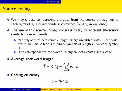
We may choose to represent the data from the source by asigning toeach symbol sk a corresponding codeword (binary, in our case).

The aim of this source coding process is to try to represent the sourcesymbols more efficiently.

◮ We only address here variable-length binary, invertible codes → the code-words are unique blocks of binary symbols of length lk , for each symbolsk .

◮ The correspondence codewords ↔ original data constitutes a code.

Average codeword length:

L = E [lk ] =K−1∑

k=0pk · lk

Coding efficiency:

η = Lmin

L≤ 1


Source coding

Shannon’s source coding theorem

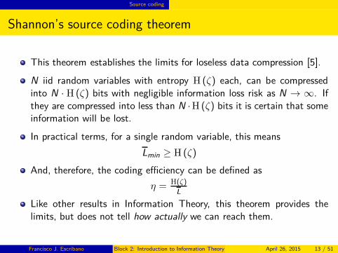
This theorem establishes the limits for loseless data compression [5].

N iid random variables with entropy H (ζ) each, can be compressedinto N · H (ζ) bits with negligible information loss risk as N → ∞. Ifthey are compressed into less than N · H (ζ) bits it is certain that someinformation will be lost.

In practical terms, for a single random variable, this means

Lmin ≥ H (ζ)

And, therefore, the coding efficiency can be defined as

η = H(ζ)

L

Like other results in Information Theory, this theorem provides thelimits, but does not tell how actually we can reach them.


Source coding

Example of source code: Huffman coding

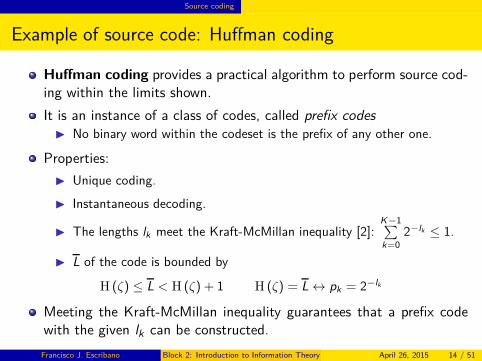
Huffman coding provides a practical algorithm to perform source cod-ing within the limits shown.

It is an instance of a class of codes, called prefix codes

◮ No binary word within the codeset is the prefix of any other one.

Properties:

◮ Unique coding.

◮ Instantaneous decoding.

◮ The lengths lk meet the Kraft-McMillan inequality [2]:K−1∑

k=0

2−lk ≤ 1.

◮ L of the code is bounded by

H (ζ) ≤ L < H (ζ) + 1 H (ζ) = L ↔ pk = 2−lk

Meeting the Kraft-McMillan inequality guarantees that a prefix codewith the given lk can be constructed.


Source coding

Huffman coding

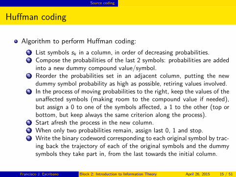
Algorithm to perform Huffman coding:

1 List symbols sk in a column, in order of decreasing probabilities.2 Compose the probabilities of the last 2 symbols: probabilities are added

into a new dummy compound value/symbol.3 Reorder the probabilities set in an adjacent column, putting the new

dummy symbol probability as high as possible, retiring values involved.4 In the process of moving probabilities to the right, keep the values of the

unaffected symbols (making room to the compound value if needed),but assign a 0 to one of the symbols affected, a 1 to the other (top orbottom, but keep always the same criterion along the process).

5 Start afresh the process in the new column.6 When only two probabilities remain, assign last 0, 1 and stop.7 Write the binary codeword corresponding to each original symbol by trac-

ing back the trajectory of each of the original symbols and the dummysymbols they take part in, from the last towards the initial column.


Source coding

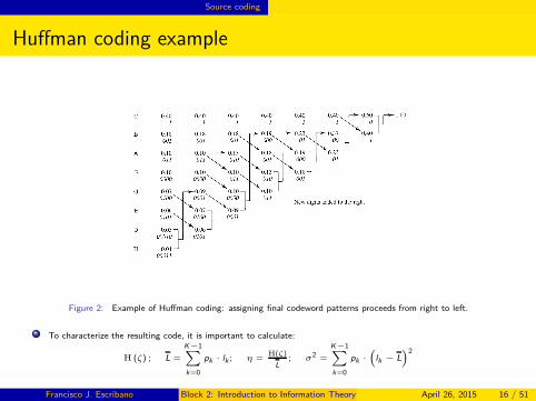
Huffman coding example

Figure 2: Example of Huffman coding: assigning final codeword patterns proceeds from right to left.

To characterize the resulting code, it is important to calculate:

H (ζ) ; L =

K−1∑

k=0

pk · lk ; η =H(ζ)

L; σ2 =

K−1∑

k=0

pk ·

(

lk − L)2


Mutual information

Mutual information


Mutual information

Joint entropy

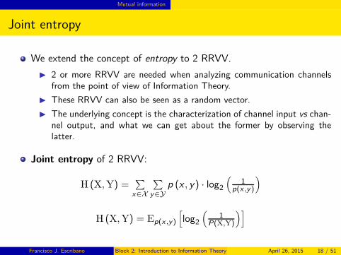
We extend the concept of entropy to 2 RRVV.

◮ 2 or more RRVV are needed when analyzing communication channelsfrom the point of view of Information Theory.

◮ These RRVV can also be seen as a random vector.

◮ The underlying concept is the characterization of channel input vs chan-nel output, and what we can get about the former by observing thelatter.

Joint entropy of 2 RRVV:

H (X, Y) =∑

x∈X

∑

y∈Yp (x , y) · log2

(

1p(x ,y)

)

H (X, Y) = Ep(x ,y)

[

log2

(

1P(X,Y)

)]


Mutual information

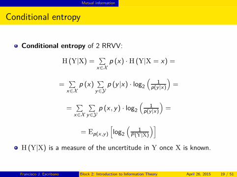
Conditional entropy

Conditional entropy of 2 RRVV:

H (Y|X) =∑

x∈Xp (x) · H (Y|X = x) =

=∑

x∈Xp (x)

∑

y∈Yp (y |x) · log2

(

1p(y |x)

)

=

=∑

x∈X

∑


(

1p(y |x)

)

=

= Ep(x ,y)

[

log2

(

1P(Y|X)

)]

H (Y|X) is a measure of the uncertitude in Y once X is known.


Mutual information

Chain rule

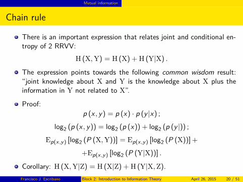
There is an important expression that relates joint and conditional en-tropy of 2 RRVV:

H (X, Y) = H (X) + H (Y|X) .

The expression points towards the following common wisdom result:“joint knowledge about X and Y is the knowledge about X plus theinformation in Y not related to X”.

Proof:

p (x , y) = p (x) · p (y |x) ;

log2 (p (x , y)) = log2 (p (x)) + log2 (p (y |)) ;

Ep(x ,y) [log2 (P (X, Y))] = Ep(x ,y) [log2 (P (X))] +

+Ep(x ,y) [log2 (P (Y|X))] .

Corollary: H (X, Y|Z) = H (X|Z) + H (Y|X, Z).


Mutual information

Relative entropy

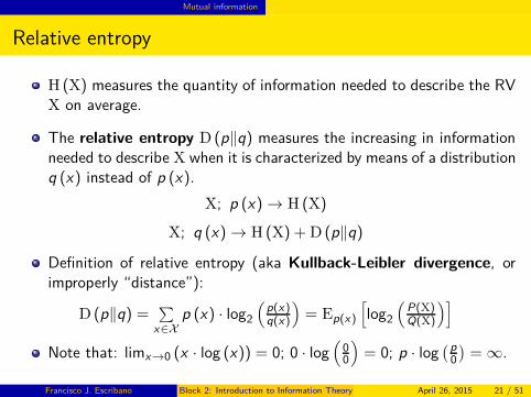
H (X) measures the quantity of information needed to describe the RVX on average.

The relative entropy D (p‖q) measures the increasing in informationneeded to describe X when it is characterized by means of a distributionq (x) instead of p (x).

X; p (x) → H (X)

X; q (x) → H (X) + D (p‖q)

Definition of relative entropy (aka Kullback-Leibler divergence, orimproperly “distance”):

D (p‖q) =∑

x∈Xp (x) · log2

(

p(x)q(x)

)

= Ep(x)

[

log2

(

P(X)Q(X)

)]

Note that: limx→0 (x · log (x)) = 0; 0 · log(

00

)

= 0; p · log( p

0

)

= ∞.


Mutual information

Relative entropy and mutual information

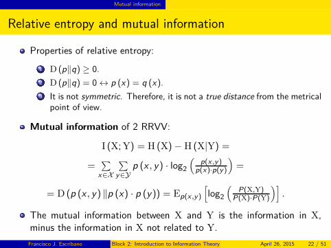
Properties of relative entropy:

1 D (p‖q) ≥ 0.

2 D (p‖q) = 0 ↔ p (x) = q (x).

3 It is not symmetric. Therefore, it is not a true distance from the metricalpoint of view.

Mutual information of 2 RRVV:

I (X; Y) = H (X) − H (X|Y) =

=∑

x∈X

∑


(

p(x ,y)p(x)·p(y)

)

=

= D (p (x , y) ‖p (x) · p (y)) = Ep(x ,y)

[

log2

(

P(X,Y)P(X)·P(Y)

)]

.

The mutual information between X and Y is the information in X,minus the information in X not related to Y.


Mutual information

Mutual information

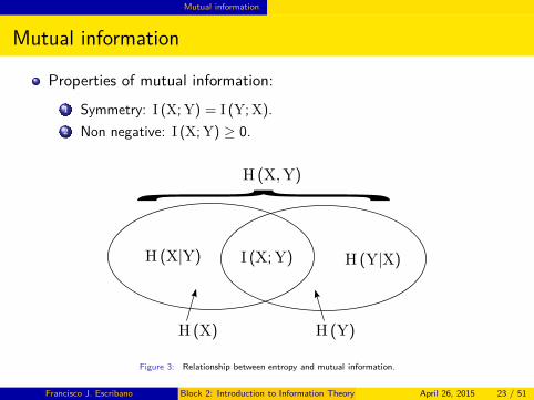
Properties of mutual information:

1 Symmetry: I (X; Y) = I (Y; X).

2 Non negative: I (X; Y) ≥ 0. }H (Y|X)I (X; Y)

H (X) H (Y)

H (X, Y)

H (X|Y)

Figure 3: Relationship between entropy and mutual information.


Discrete channels

Discrete channels


Discrete channels

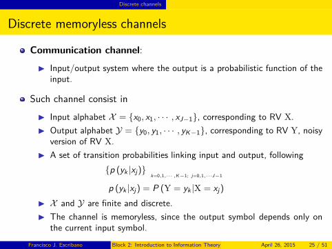
Discrete memoryless channels

Communication channel:

◮ Input/output system where the output is a probabilistic function of theinput.

Such channel consist in

◮ Input alphabet X = {x0, x1, · · · , xJ−1}, corresponding to RV X.

◮ Output alphabet Y = {y0, y1, · · · , yK−1}, corresponding to RV Y, noisyversion of RV X.

◮ A set of transition probabilities linking input and output, following

{p (yk |xj)}k=0,1,··· ,K−1; j=0,1,···J−1

p (yk |xj) = P (Y = yk |X = xj)

◮ X and Y are finite and discrete.

◮ The channel is memoryless, since the output symbol depends only onthe current input symbol.


Discrete channels


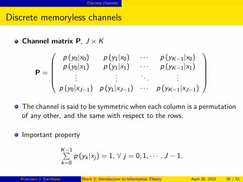
Channel matrix P, J × K

P =

p (y0|x0) p (y1|x0) · · · p (yK−1|x0)p (y0|x1) p (y1|x1) · · · p (yK−1|x1)

......

. . ....

p (y0|xJ−1) p (y1|xJ−1) · · · p (yK−1|xJ−1)

The channel is said to be symmetric when each column is a permutationof any other, and the same with respect to the rows.

Important property

K−1∑

k=0p (yk |xj) = 1, ∀ j = 0, 1, · · · , J − 1.


Discrete channels


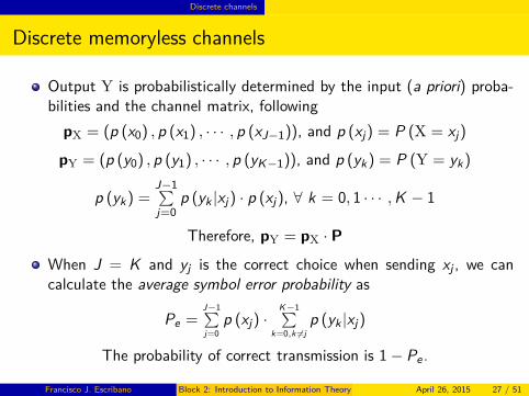
Output Y is probabilistically determined by the input (a priori) proba-bilities and the channel matrix, following

pX = (p (x0) , p (x1) , · · · , p (xJ−1)), and p (xj) = P (X = xj)

pY = (p (y0) , p (y1) , · · · , p (yK−1)), and p (yk) = P (Y = yk)

p (yk) =J−1∑

j=0p (yk |xj) · p (xj), ∀ k = 0, 1 · · · , K − 1

Therefore, pY = pX · P

When J = K and yj is the correct choice when sending xj , we cancalculate the average symbol error probability as

Pe =J−1∑

j=0

p (xj) ·K−1∑

k=0,k 6=j

p (yk |xj)

The probability of correct transmission is 1 − Pe .


Discrete channels


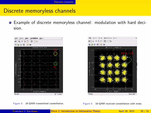
Example of discrete memoryless channel: modulation with hard deci-sion.

xj

yk

Figure 4: 16-QAM transmitted constellation.

p(yk |xj)

Figure 5: 16-QAM received constellation with noise.


Discrete channels

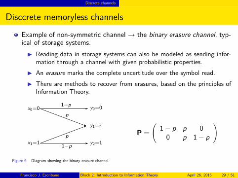
Disccrete memoryless channels

Example of non-symmetric channel → the binary erasure channel, typ-ical of storage systems.

◮ Reading data in storage systems can also be modeled as sending infor-mation through a channel with given probabilistic properties.

◮ An erasure marks the complete uncertitude over the symbol read.

◮ There are methods to recover from erasures, based on the principles ofInformation Theory.

x0=0

x1=1

y0=0

y1=ǫ

y2=11−p

1−p

p

p

Figure 6: Diagram showing the binary erasure channel.

P =

(

1 − p p 00 p 1 − p

)


Discrete channels

Channel capacity

Mutual information depends on P and pX. Characterizing the possibil-ities of the channel requires removing dependency with pX.

Channel capacity is defined as

C = maxpXI (X; Y)

◮ This is the maximum average mutual information enabled by the channel,in bits per channel use, and the best we can get out of it in point ofreliable information transfer.

◮ It only depends on the channel transition probabilities P.

◮ If the channel is symmetric, the distribution that maximizes I (X; Y) isthe uniform one (equiprobable symbols).

Channel coding is a process where controled redundancy is added toprotect data integrity.

◮ A channel encoded information sequence has n bits, encoded from ablock of k information bits → the code rate is calculated as R = k

n ≤ 1.


Discrete channels

Noisy-channel coding theorem

Consider a discrete source ζ, emitting symbols with period Ts .

◮ The binary information rate of such source is H(ζ)Ts

(bit/s).

Consider a discrete memoryless channel, used to send coded data eachTc seconds.

◮ The maximum possible data transfer rate would be C

Tc(bit/s).

The noisy-channel coding theorem states the following [5]:

◮ If H(ζ)Ts

≤ C

Tc, there exists a coding scheme that guarantees errorfree

transmission (i.e. Pe arbitrarily small).

◮ Conversely, if H(ζ)Ts

> C

Tc, the communication cannot be made reliable

(i.e. we cannot have a bounded Pe , so small as desired).

Please note that again the theorem is asymptotic, and not constructive:it does not say how to actually reach the limit.


Discrete channels


Example: a binary symmetric channel.

Consider a binary source ζ = {0, 1}, with equiprobable symbols.

◮ H (ζ) = 1 info bits/“channel use”.

◮ Source works at a rate of 1Ts

“channel uses”/s, and H(ζ)Ts

info bits/s.

Consider an encoder with rates kn info/coded bits, and 1

Tc“channel

uses”/s.

◮ Note that kn = Tc

Ts.

Maximum achievable rate is C

Tccoded bits/s.

If H(ζ)Ts

= 1Ts

≤ C

Tc, we could find a coding scheme so that Pe is made

arbitrarily small (so small as desired).

◮ This means that an appropriate coding scheme has to meet kn ≤ C in

order to exploit the possibilities of the noisy-channel coding theorem.


Discrete channels


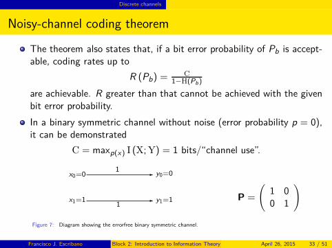
The theorem also states that, if a bit error probability of Pb is accept-able, coding rates up to

R (Pb) = C

1−H(Pb)

are achievable. R greater than that cannot be achieved with the givenbit error probability.

In a binary symmetric channel without noise (error probability p = 0),it can be demonstrated

C = maxp(x) I (X; Y) = 1 bits/“channel use”.

x0=0

x1=1

y0=0

y1=11

1

Figure 7: Diagram showing the errorfree binary symmetric channel.

P =

(

1 00 1

)


Discrete channels


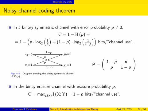
In a binary symmetric channel with error probability p 6= 0,

C = 1 − H (p) =

= 1 −(

p · log2

(

1p

)

+ (1 − p) · log2

(

11−p

))

bits/“channel use”.

replacements

x0=0

x1=1

y0=0

y1=11−p

1−p

p

p

Figure 8: Diagram showing the binary symmetric channel-BSC(p).

P =

(

1 − p p

p 1 − p

)

In the binay erasure channel with erasure probability p,

C = maxp(x) I (X; Y) = 1 − p bits/“channel use”.


Entropy and mutual information for continuous RRVV

Entropy and mutual information

for continuous RRVV



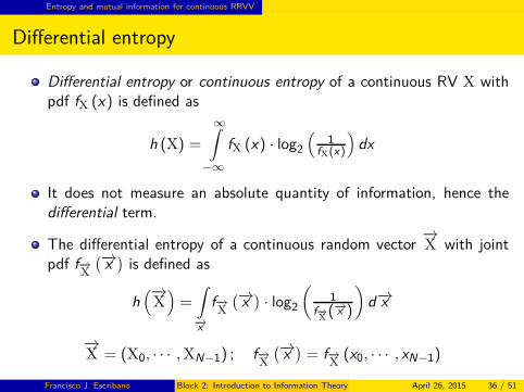
Differential entropy

Differential entropy or continuous entropy of a continuous RV X withpdf fX (x) is defined as

h (X) =

∞∫

−∞

fX (x) · log2

(

1fX(x)

)

dx

It does not measure an absolute quantity of information, hence thedifferential term.

The differential entropy of a continuous random vector−→X with joint

pdf f−→X

(−→x)

is defined as

h(−→

X)

=

∫

−→x

f−→X

(−→x)

· log2

(

1f−→

X(−→x )

)

d−→x

−→X = (X0, · · · , XN−1) ; f−→

X

(−→x)

= f−→X

(x0, · · · , xN−1)



Differential entropy

For a given variance value σ2, the Gaussian RV exhibits the largestachievable differential entropy.

◮ This means the Gaussian RV has a special place in the domain of con-tinuous RRVV within Information Theory.

Properties of differential entropy

◮ Differential entropy is invariant under translations

h (X + c) = h (X)

◮ Scaling

h (a · X) = h (X) + log2 (|a|)

h(

A ·−→X)

= h(−→

X)

+ log2 (|A|)

◮ For given variance σ2, a Gaussian RV X with variance σ2X

= σ2 and anyother RV Y with variance σ2

Y= σ2, h (X) ≥ h (Y).

◮ For a Gaussian RV X with variance σ2X

h (X) = 12 log2

(

2π e σ2X

)



Mutual information for continuous RRVV

Mutual information of two continuous RRVV X and Y

I (X; Y) =

∞∫

−∞

∞∫

−∞

fX,Y (x , y) · log2

(

fX(x |y)fX(x)

)

dxdy

fX,Y (x , y) is X and Y joint pdf, and fX (x |y) is the conditional pdf ofX given Y = y .

Properties

◮ Symmetry, I (X; Y) = I (Y; X).

◮ Non-negative, I (X; Y) ≥ 0.

◮ I (X; Y) = h (X) − h (X|Y).

◮ I (X; Y) = h (Y) − h (Y|X).

h (X|Y) =

∞∫

−∞

∞∫

−∞

fX,Y (x , y) · log2

(

1fX(x |y)

)

dxdy

This is the conditional differential entropy of X given Y.


Channel capacity theorem




Continuous channel capacity

Gaussian discrete memoryless channel, described by

◮ x(t) is a stocastic stationary process, with mx = 0 and bandwidth Wx =B Hz.

◮ Process is sampled at sampling rate Ts = 12B , and Xk = x (k · Ts) are

thus a bunch of continuous RRVV ∀ k , with E [Xk ] = 0.

◮ A RV Xk is transmitted each Ts seconds over a noisy channel withbandwidth B, during a total of T seconds (n = 2BT total samples).

◮ The channel is AWGN, adding noise samples described by RRVV Nk

with mn = 0 and Sn (f ) = N0

2 , so that σ2n = N0B.

◮ The received samples are statistically independent RRVV, described asYk = Xk + Nk .

◮ The cost function for any maximization of the mutual information is thesignal power E

[

X2k

]

= S.



Continuous channel capacity

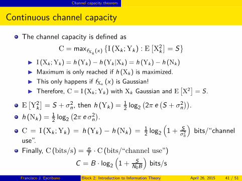
The channel capacity is defined as

C = maxfXk(x)

{

I (Xk ; Yk) : E[

X2k

]

= S}

◮ I (Xk ; Yk) = h (Yk) − h (Yk |Xk) = h (Yk) − h (Nk)

◮ Maximum is only reached if h (Xk) is maximized.

◮ This only happens if fXk(x) is Gaussian!

◮ Therefore, C = I (Xk ; Yk) with Xk Gaussian and E[

X2]

= S.

E[

Y2k

]

= S + σ2n, then h (Yk) = 1

2 log2

(

2π e(

S + σ2n

))

.

h (Nk) = 12 log2

(

2π e σ2n

)

.

C = I (Xk ; Yk) = h (Yk) − h (Nk) = 12 log2

(

1 + Sσ2

n

)

bits/“channel

use”.

Finally, C (bits/s) = nT · C (bits/“channel use”)

C = B · log2

(

1 + SN0B

)

bits/s



Shannon-Hartley theorem

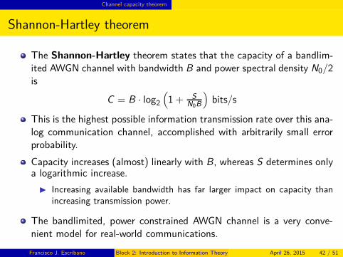
The Shannon-Hartley theorem states that the capacity of a bandlim-ited AWGN channel with bandwidth B and power spectral density N0/2is

C = B · log2

(

1 + SN0B

)

bits/s

This is the highest possible information transmission rate over this ana-log communication channel, accomplished with arbitrarily small errorprobability.

Capacity increases (almost) linearly with B, whereas S determines onlya logarithmic increase.

◮ Increasing available bandwidth has far larger impact on capacity thanincreasing transmission power.

The bandlimited, power constrained AWGN channel is a very conve-nient model for real-world communications.



Implications of the channel capacity theorem

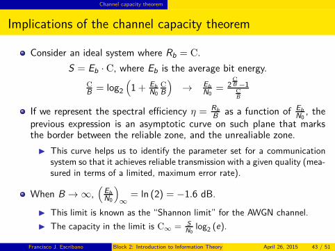
Consider an ideal system where Rb = C.

S = Eb · C, where Eb is the average bit energy.

C

B = log2

(

1 + EbN0

C

B

)

→ EbN0

= 2CB −1CB

If we represent the spectral efficiency η = RbB as a function of Eb

N0, the

previous expression is an asymptotic curve on such plane that marksthe border between the reliable zone, and the unrealiable zone.

◮ This curve helps us to identify the parameter set for a communicationsystem so that it achieves reliable transmission with a given quality (mea-sured in terms of a limited, maximum error rate).

When B → ∞,(

EbN0

)

∞= ln (2) = −1.6 dB.

◮ This limit is known as the “Shannon limit” for the AWGN channel.

◮ The capacity in the limit is C∞ = SN0

log2 (e).



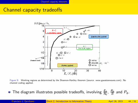
Channel capacity tradeoffs

Figure 9: Working regions as determined by the Shannon-Hartley theorem (source: www.gaussianwaves.com). Nochannel coding applied.

The diagram illustrates possible tradeoffs, involving EbN0

, RbB and Pb.




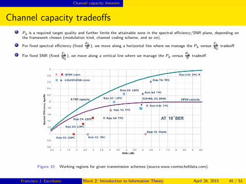
Pb is a required target quality and further limits the attainable zone in the spectral efficiency/SNR plane, depending onthe framework chosen (modulation kind, channel coding scheme, and so on).

For fixed spectral efficiency (fixedRbB

), we move along a horizontal line where we manage the Pb versusEbN0

tradeoff.

For fixed SNR (fixedEbN0

), we move along a vertical line where we manage the Pb versusRbB

tradeoff.

Figure 10: Working regions for given transmission schemes (source:www.comtechefdata.com).




The lower, left hand side of the plot is the so-called power limitedregion.

◮ There, the Eb

N0is very poor and we have to sacrifice spectral efficiency to

get a given transmission quality (Pb).

◮ An example of this are deep space communications, where the SNRreceived is extremely low due to the huge free space losses in the link.The only way to get a reliable transmission is to drop data rate at verylow values.

The upper, right hand side of the plot is de so-called bandwidth limitedregion.

◮ There, the desired spectral efficiency Rb

B for fixed B (desired data rate)is traded-off against unconstrained transmission power (unconstrainedEb

N0), under a given Pb.

◮ An example of this would be a terrestrial DVB transmitting station,where Rb

B is fixed (standarized), and where the transmitting power isonly limited by regulatory or technological constraints.


Conclusions

Conclusions


Conclusions

Conclusions

Information Theory represents a cutting-edge research field with appli-cations in communications, artificial intelligence, data mining, machinelearning, robotics...

We have seen three fundamental results from Shannon’s 1948 seminalwork, that constitute the foundations of all modern communications.

◮ Source coding theorem, that states the limits and possibilities of loss-less data compresion.

◮ Noisy-channel coding theorem, that states the need of channel codingtechniques to achieve a given performance, using constrained resources.It establishes the asymptotic possibility of errorfree transmission overdiscrete-input discrete-output noisy channels.

◮ Shannon-Hartley theorem, which establishes the absolute (asymp-totic) limits for errorfree transmission over AWGN channels, and de-scribes the different tradeoffs involved among the given resources.


Conclusions

Conclusions

All these results build the attainable working zone for practical andfeasible communication systems, managing and trading-off constrainedresources and under a given target performance (BER).

◮ The η = Rb

B against Eb

N0plane (under a target BER) constitutes the

playground for designing and bringing into practice any communicationstandards.

◮ Any movement over the plane has a direct impact over business andrevenues in the telco domain.

When addressing practical designs in communications, these results andlimits are not much heeded, but they underlie all of them.

◮ There are lots of common practice and common wisdom rules of thumbin the domain, stating what to use when (regarding modulations, channelencoders and so on).

◮ Nevertheless, optimizing the designs so as to profit as much as possiblefrom all the resources at hand require making these limits explicit.


References

References


References

Bibliography I

[1] J. M. Cioffi, Digital Communications - coding (course). Stanford University, 2010. [Online]. Available:http://web.stanford.edu/group/cioffi/book

[2] T. M. Cover and J. A. Thomas, Elements of Information Theory. New Jersey: John Wiley & Sons, Inc., 2006.

[3] D. MacKay, Information Theory, Inference, and Learning Algorithms. Cambridge University Press, 2003. [Online]. Available:http://www.inference.phy.cam.ac.uk/mackay/itila/book.html

[4] S. Haykin, Communications Systems. New York: John Wiley & Sons, Inc., 2001.

[5] Claude E. Shannon, “A mathematical theory of communication,” Bell Systems Technical Journal. [Online]. Available:http://plan9.bell-labs.com/cm/ms/what/shannonday/shannon1948.pdf


http://web.stanford.edu/group/cioffi/book

http://www.inference.phy.cam.ac.uk/mackay/itila/book.html

http://plan9.bell-labs.com/cm/ms/what/shannonday/shannon1948.pdf

Documents

Block 2: Introduction to Information Theory · Block 2: Introduction to Information Theory ... 3 Source coding 4 Mutual information 5 Discrete channels 6 Entropy and mutual information