Int J Speech Technol (2010) 13: 1–12DOI 10.1007/s10772-010-9066-0

Blind separation of audio signals using trigonometric transformsand wavelet denoising

Hossam Hammam · Atef Abou Elazm ·Mohamed E. Elhalawany · Fathi E. Abd El-Samie

Received: 20 April 2009 / Accepted: 10 February 2010 / Published online: 3 March 2010© Springer Science+Business Media, LLC 2010

Abstract This paper deals with the problem of blind sep-aration of audio signals from noisy mixtures. It proposesthe application of a blind separation algorithm on the dis-crete cosine transform (DCT) or the discrete sine transform(DST) of the mixed signals, instead of performing the sepa-ration on the mixtures in the time domain. Wavelet denois-ing of the noisy mixtures is recommended in this paper asa preprocessing step for noise reduction. Both the DCT andthe DST have an energy compaction property, which con-centrates most of the signal energy in a few coefficients inthe transform domain, leaving most of the transform domaincoefficients close to zero. As a result, the separation is per-formed on a few coefficients in the transform domain. An-other advantage of signal separation in transform domainsis that the effect of noise on the signals in the transform do-mains is smaller than that in the time domain due to the av-eraging effect of the transform equations, especially whenthe separation algorithm is preceded by a wavelet denoisingstep. The simulation results confirm the superiority of trans-form domain separation to time domain separation and theimportance of the wavelet denoising step.

H. HammamTelecom Egypt, Alexandria, Egypte-mail: hossammha@yahoo.com

A.A. Elazm · M.E. Elhalawany · F.E. Abd El-Samie (�)Department of Electronics and Electrical Communications,Faculty of Electronic Engineering, Menoufia University,Menouf 32952, Egypte-mail: fathi_sayed@yahoo.com

A.A. Elazme-mail: abouelazm_atef@yahoo.com

M.E. Elhalawanye-mail: halawany_m85@yahoo.com

Keywords DCT · DST · Wavelet denoising · Signalseparation

1 Introduction

Blind signal separation is an important branch of signalprocessing. It deals mainly with mixed signals, which arefrequently encountered in real life. Real life signals are fre-quently mixed with undesired signals. This fact has moti-vated the evolution of blind signal separation algorithms.The word blind means that there is no a priori informa-tion about the mixed signals and there sources. Several ap-proaches have been proposed for blind signal separation(Sakai and Mitsuhashi 2008; Dam et al. 2007, 2008; Man-montri and Naylor 2008; Curnew and How 2007; Szupiluket al. 2006; Moreau et al. 2007; Won and Lee 2008). Some ofthese approaches depend on independent component analy-sis. Other approaches depend on higher order statistics.There is also a category of correlation based separation al-gorithms. Adaptive signal separation algorithms also exist.

Generally, most of the separation algorithms deal withthe problem in the presence of noise. The existence of noisecauses some deterioration in the quality of the separated sig-nals. As a result, there is a need for a technique to reduce theeffect of noise on the separation process. Wavelet denois-ing is well known as an effective denoising technique (Proc-hazka et al. 1998; Walker 1999). This technique is based onthe decomposition of the noisy signal into sub-bands andneglecting samples of less importance in the high frequencysub-bands, which may be due to noise. This process has theeffect of reducing the noise effect on the signal. The signaldecomposed into sub-bands is then reconstructed again us-ing an inverse wavelet transform.

2 Int J Speech Technol (2010) 13: 1–12

This paper proposes the application of wavelet denoisingon the noisy mixtures as a preprocessing step, then the appli-cation of the blind signal separation algorithm after applyingthe DCT or the DST on the denoised mixtures. The rest ofthe paper is organized as follows. Sections 2 and 3 presentthe blind signal separation algorithm. Section 4 gives theprinciples of wavelet denoising. Section 5 gives the trigono-metric transforms. Section 6 introduces some metrics to as-sess the perceptual quality of the separated audio signals.Section 7 gives the simulation results. Finally, the conclud-ing remarks are given in Sect. 8.

2 Problem formulation

Blind signal separation deals with mixtures of signals in thepresence of noise. If there are two original signals s1(k) ands2(k), which are mixed together to give two observationsx1(k) and x2(k), these observations can be represented asfollows (Chan 1997):

x1(k) =p∑

i=0

h11(i)s1(k − i)

+p∑

i=0

h12(i)s2(k − i) + v1(k)

x2(k) =p∑

i=0

h21(i)s1(k − i)

+p∑

i=0

h22(i)s2(k − i) + v2(k)

(1)

or in matrix form as follows:(

x1(k)

x2(k)

)=

(hT

11 hT12

hT21 hT

22

)(s1(k)

s2(k)

)+

(v1(k)

v2(k)

)(2)

where

hTij = [

hij (0), . . . , hij (p)]

sTi (k) = [

si(k), . . . , si(k − p)] (3)

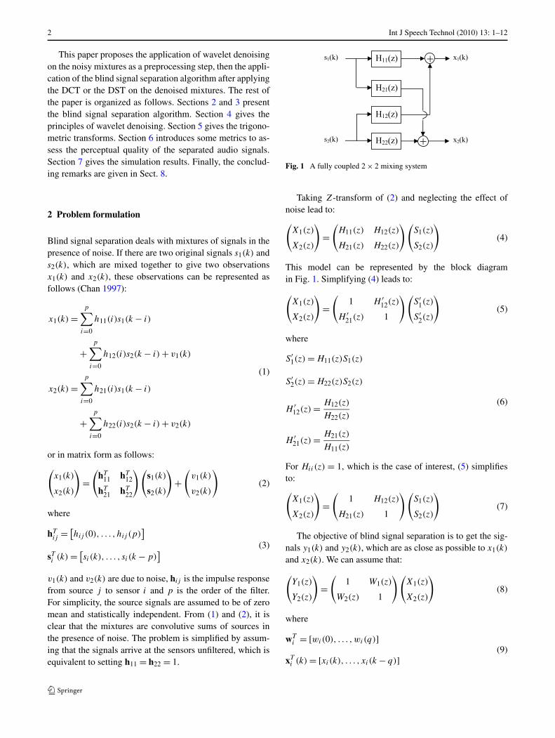
v1(k) and v2(k) are due to noise, hij is the impulse responsefrom source j to sensor i and p is the order of the filter.For simplicity, the source signals are assumed to be of zeromean and statistically independent. From (1) and (2), it isclear that the mixtures are convolutive sums of sources inthe presence of noise. The problem is simplified by assum-ing that the signals arrive at the sensors unfiltered, which isequivalent to setting h11 = h22 = 1.

Fig. 1 A fully coupled 2 × 2 mixing system

Taking Z-transform of (2) and neglecting the effect ofnoise lead to:(

X1(z)

X2(z)

)=

(H11(z) H12(z)

H21(z) H22(z)

)(S1(z)

S2(z)

)(4)

This model can be represented by the block diagramin Fig. 1. Simplifying (4) leads to:

(X1(z)

X2(z)

)=

(1 H ′

12(z)

H ′21(z) 1

)(S′

1(z)

S′2(z)

)(5)

where

S′1(z) = H11(z)S1(z)

S′2(z) = H22(z)S2(z)

H ′12(z) = H12(z)

H22(z)

H ′21(z) = H21(z)

H11(z)

(6)

For Hii(z) = 1, which is the case of interest, (5) simplifiesto:(

X1(z)

X2(z)

)=

(1 H12(z)

H21(z) 1

)(S1(z)

S2(z)

)(7)

The objective of blind signal separation is to get the sig-nals y1(k) and y2(k), which are as close as possible to x1(k)

and x2(k). We can assume that:

(Y1(z)

Y2(z)

)=

(1 W1(z)

W2(z) 1

)(X1(z)

X2(z)

)(8)

where

wTi = [wi(0), . . . ,wi(q)]

xTi (k) = [xi(k), . . . , xi(k − q)]

(9)

Int J Speech Technol (2010) 13: 1–12 3

Substituting (7) into (8) leads to Chan (1997):

(Y1(z)

Y2(z)

)=

(1 + W1(z)H21(z) W1(z) + H12(z)

W2(z) + H21(z) 1 + W2(z)H12(z)

)

×(

S1(z)

S2(z)

)(10)

3 Block based separation algorithm

This section deals with a time domain iterative separa-tion algorithm for the 2 × 2 convolutive system. The algo-rithm minimizes the output cross-correlations for an arbi-trary number of lags with q + 1 tap FIR filters. From (9),it is clear that the solution of the problem is to find suitableW1(z) and W2(z), such that each of Y1(z) and Y2(z) containsonly S1(z) or S2(z). This is achieved only if either the diag-onal or the anti-diagonal elements of the cross-correlationmatrices are zeros.

Assuming s1(k) and s2(k) are stationary, zero mean andindependent random signals, the cross-correlation betweenthe two signals is equal to zero, that is (Chan 1997):

rs1s2(l) = E[s1(k)s2(k + l)] = 0 ∀l (11)

If each of y1(k) and y2(k) contains components of s1(k)

or s2(k) only, then the cross-correlation between y1(k) andy2(k) should also be zero, then:

ry1y2(l) = E[y1(k)y2(k + l)] = 0 ∀l (12)

Substituting (8) into (12) gives:

ry1y2(l) = E[(x1(k) + wT1 x2(k))

× (x2(k + l) + wT2 x1(k + 1))] (13)

If rxixj(l) = E[xi(k)xj (k + l)], (13) becomes:

ry1y2(l) = rx1x2(l) + wT1

⎛

⎜⎝rx2x2(l)

...

rx2x2(l + q)

⎞

⎟⎠

+ wT2

⎛

⎜⎝rx1x1(l)

...

rx1x1(l + q)

⎞

⎟⎠ + wT1 Rx2x1(l)w2 (14)

where Rx2x1(l) = E[x2(k)(x1(k+ l))T ] is a (q +1)×(q +1)

matrix, which is a function of the cross-correlation betweenx1 and x2.

The cost function C is defined as the sum of the squaresof the cross-correlations between the two inputs as follows

Fig. 2 Schematic diagram of the 2 × 2 separation algorithm

(Chan 1997):

C =l2∑

l=l1

[ry1y2(l)

]2 (15)

where l1 and l2 constitute a range of cross-correlation lags.C can also be expressed as

C = rTy1y2

ry1y2 (16)

where

ry1y2 = [ry1y2(l1), . . . , ry1y2(l2)]T (17)

Thus

ry1y2 = rx1x2 + [Q+x2x2

]T w1 + [Q−x1x1

]T w2

+ RTx2x1

A(w2)w1 (18)

or

ry1y2 = rx1x2 + [Q+x2x2

]T w1 + [Q−x1x1

]T w2

+ RTx1x2

A(w1)w2 (19)

where Q+x2x2

and Q−x1x1

are (q + 1) × (l2 − l1 + 1) ma-trices, Rx2x1 is a (2q + 1) × (l2 − l1 + 1) matrix. Theseare all correlation matrices of x1 and x2 and are estimatedusing sample correlation estimates. A(w1) and A(w2) are(2q + 1) × (q + 1) matrices, which contain w1 and w2, re-spectively. In order to find some suitable w1 and w2,C isminimized such that:

∂C

∂wk

= [0, . . . ,0]T , k = 1,2 (20)

Let

ψ1 = ([Q+x2x2

]T + RTx2x1

A(w2))

ψ2 = ([Q−x1x1

]T + RTx1x2

A(w1))

(21)

Substituting (21) into (18) and (19) gives:

ry1y2 = rx1x2 + ψ1w1 + [Q−x1x1

]T w2 (22)

4 Int J Speech Technol (2010) 13: 1–12

or

ry1y2 = rx1x2 + ψ2w2 + [Q+x2x2

]T w1 (23)

From (20), we obtain (Chan 1997):

w1 = −(ψT1 ψ1)

−1ψT1 (rx1x2 + [Q−

x1x1]T w2)

w2 = −(ψT2 ψ2)

−1ψT2 (rx1x2 + [Q+

x2x2]T w1)

(24)

w1 and w2 can be obtained by iterating between the twoequations until convergence is achieved, when the rate ofchange of parameter values is less than a pre-set threshold.By estimating w1 and w2, we then obtain a set of outputsy1(k) and y2(k). Each output contains s1(k) or s2(k), only.

4 Wavelet denoising

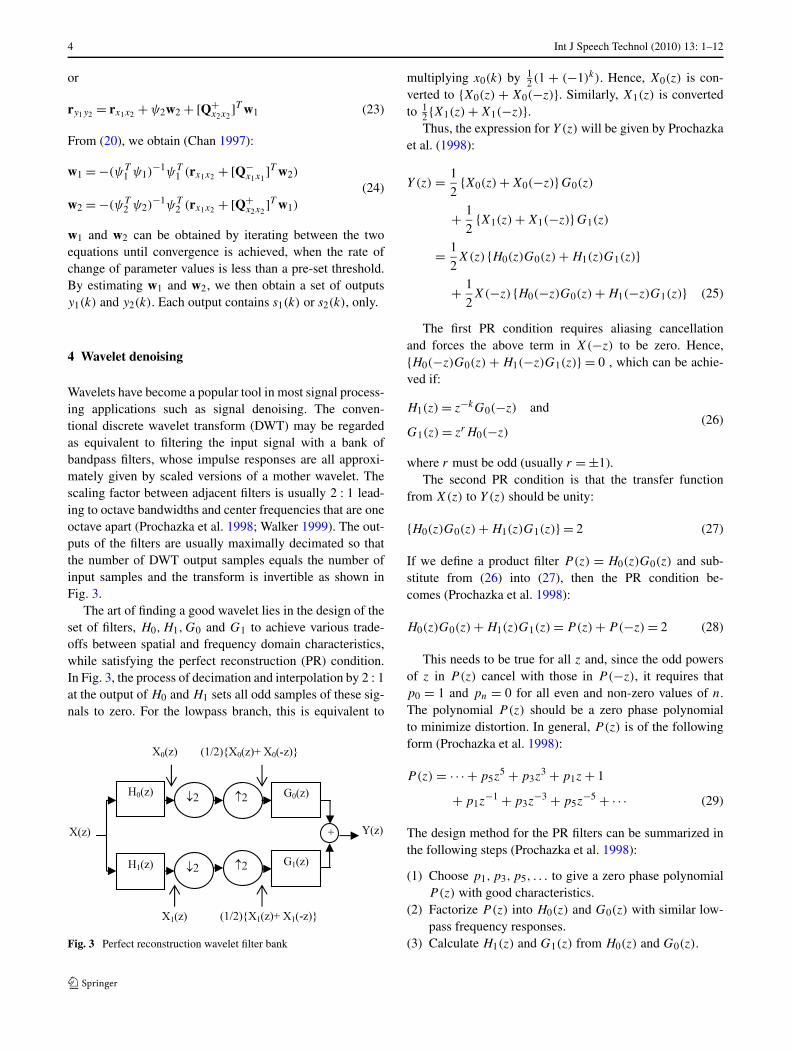
Wavelets have become a popular tool in most signal process-ing applications such as signal denoising. The conven-tional discrete wavelet transform (DWT) may be regardedas equivalent to filtering the input signal with a bank ofbandpass filters, whose impulse responses are all approxi-mately given by scaled versions of a mother wavelet. Thescaling factor between adjacent filters is usually 2 : 1 lead-ing to octave bandwidths and center frequencies that are oneoctave apart (Prochazka et al. 1998; Walker 1999). The out-puts of the filters are usually maximally decimated so thatthe number of DWT output samples equals the number ofinput samples and the transform is invertible as shown inFig. 3.

The art of finding a good wavelet lies in the design of theset of filters, H0,H1,G0 and G1 to achieve various trade-offs between spatial and frequency domain characteristics,while satisfying the perfect reconstruction (PR) condition.In Fig. 3, the process of decimation and interpolation by 2 : 1at the output of H0 and H1 sets all odd samples of these sig-nals to zero. For the lowpass branch, this is equivalent to

Fig. 3 Perfect reconstruction wavelet filter bank

multiplying x0(k) by 12 (1 + (−1)k). Hence, X0(z) is con-

verted to {X0(z) + X0(−z)}. Similarly, X1(z) is convertedto 1

2 {X1(z) + X1(−z)}.Thus, the expression for Y(z) will be given by Prochazka

et al. (1998):

Y(z) = 1

2{X0(z) + X0(−z)}G0(z)

+ 1

2{X1(z) + X1(−z)}G1(z)

= 1

2X(z) {H0(z)G0(z) + H1(z)G1(z)}

+ 1

2X(−z) {H0(−z)G0(z) + H1(−z)G1(z)} (25)

The first PR condition requires aliasing cancellationand forces the above term in X(−z) to be zero. Hence,{H0(−z)G0(z) + H1(−z)G1(z)} = 0 , which can be achie-ved if:

H1(z) = z−kG0(−z) and

G1(z) = zrH0(−z)(26)

where r must be odd (usually r = ±1).The second PR condition is that the transfer function

from X(z) to Y(z) should be unity:

{H0(z)G0(z) + H1(z)G1(z)} = 2 (27)

If we define a product filter P(z) = H0(z)G0(z) and sub-stitute from (26) into (27), then the PR condition be-comes (Prochazka et al. 1998):

H0(z)G0(z) + H1(z)G1(z) = P(z) + P(−z) = 2 (28)

This needs to be true for all z and, since the odd powersof z in P(z) cancel with those in P(−z), it requires thatp0 = 1 and pn = 0 for all even and non-zero values of n.The polynomial P(z) should be a zero phase polynomialto minimize distortion. In general, P(z) is of the followingform (Prochazka et al. 1998):

P(z) = · · · + p5z5 + p3z

3 + p1z + 1

+ p1z−1 + p3z

−3 + p5z−5 + · · · (29)

The design method for the PR filters can be summarized inthe following steps (Prochazka et al. 1998):

(1) Choose p1,p3,p5, . . . to give a zero phase polynomialP(z) with good characteristics.

(2) Factorize P(z) into H0(z) and G0(z) with similar low-pass frequency responses.

(3) Calculate H1(z) and G1(z) from H0(z) and G0(z).

Int J Speech Technol (2010) 13: 1–12 5

To simplify this procedure, we can use the following re-lation:

P(z) = Pt (Z) = 1 + pt,1Z + pt,3Z3 + pt,5Z

5 + · · · (30)

where

Z = 1

2(z + z−1) (31)

For wavelet denoising, we will use the Haar wavelet, whichis the simplest type of wavelets. In discrete form, the Haarwavelet is related to a mathematical operation called theHaar transform. The Haar transform serves as a prototypefor all other wavelet transforms. This transform decomposesa discrete signal into two sub-signals of half its length. Onesub-signal is a running average or trend and the other sub-signal is a running difference or fluctuation.

This uses the simplest possible Pt (Z) with a single zeroat Z = −1, which is represented as follows:

Pt(Z) = 1 + Z (32)

Thus

P(z) = 1

2(z + 2 + z−1) = 1

2(z + 1)(1 + z−1)

= G0(z)H0(z) (33)

We can find H0(z) and G0(z) as follows (Prochazka et al.1998):

H0(z) = 1

2(1 + z−1) (34)

G0(z) = (z + 1) (35)

Using (26) with r = 1:

G1(z) = zH0(−z) = 1

2z(1 − z−1) = 1

2(z − 1) (36)

H1(z) = z−1G0(−z) = z−1(−z + 1) = (z−1 − 1) (37)

Wavelet denoising is a simple operation which aims at re-ducing noise in a noisy signal. It is performed by choosing athreshold that is a sufficiently large multiple of the standarddeviation of the noise in the signal. Most of the noise poweris removed by thresholding the high frequency wavelettransform coefficients. There are two types of thresholding;hard and soft thresholding. The equation of the hard thresh-olding is given by Walker (1999):

fhard(x) ={

x |x| ≥ T

0 |x| < T(38)

On the other hand, that of soft thresholding is given byWalker (1999):

fsoft(x) =

⎧⎪⎪⎪⎪⎨

⎪⎪⎪⎪⎩

x |x| ≥ T

2x − T T/2 ≤ x < T

T + 2x −T < x ≤ −T/2

0 |x| < T/2

(39)

T denotes the threshold value and x represents the coeffi-cients of the high frequency components of the DWT. Wewill use soft thresholding in this paper, because it has a bet-ter performance than hard thresholding.

5 Trigonometric transforms

Trigonometric transforms include the DCT and the DST. Itis known that these transforms have an energy compactionproperty. The effect of noise is reduced in these transformsdue to the averaging process in the transform equations. As aresult, signal separation in these transform domains can givebetter results than in the time domain. In the following sub-sections, a brief explanation of these transforms is presented.

5.1 The DCT

The DCT expresses the samples of a signal in terms of a sumof cosine functions oscillating at different frequencies. TheDCT is defined by the following equation (Prochazka et al.1998):

X(m) = w(m)

K−1∑

k=0

x(k) cos

(π(2k − 1)(m − 1)

2K

)

m = 0, . . . ,K − 1 (40)

where x(k) is the signal with length K .

w(m) =⎧⎨

⎩

1√K

m = 0√

2K

m = 1, . . . ,K − 1(41)

5.2 The DST

The DST is similar to the DCT, but it uses sine functionsoscillating at different frequencies rather than cosine func-tions. The DST is defined by the following equation (Proc-hazka et al. 1998):

X(m) =K−1∑

k=0

x(k) sin

(πmk

K + 1

)m = 0, . . . ,K − 1 (42)

6 Int J Speech Technol (2010) 13: 1–12

6 Objective quality metrics for audio signals

There is a need of some metrics to assess the perceptualquality of the audio signals resulting from any signal separa-tion algorithm. Several approaches, based on subjective andobjective metrics, have been adopted in the literature for thispurpose (Kubichek 1993; Wang et al. 1992; Yang et al. 1998;Crochiere et al. 1980). Concentration in this paper will be onthe objective metrics.

Objective metrics are generally divided into intrusive andnon-intrusive metrics. Intrusive metrics can be classified intothree main groups. The first group includes time domainmetrics such as the traditional signal-to-noise ratio (SNR)and segmental signal-to-noise ratio (SNRseg). The secondgroup includes linear predictive coefficients (LPCs) met-rics, which are based on the LPCs of the audio signal andits derivative parameters, such as the linear reflection co-efficients (LRCs), the log likelihood ratio (LLR), and thecepstral distance (CD). The third group includes the spec-tral domain metrics, which are based on the comparisonbetween the power spectrum of the original signal and theprocessed signal. An example of such metrics is the spec-tral distortion (SD) (Kubichek 1993; Wang et al. 1992;Yang et al. 1998; Crochiere et al. 1980).

6.1 The SNR

The SNR is defined as follows (Kubichek 1993; Wang et al.1992; Yang et al. 1998; Crochiere et al. 1980):

SNR = 10 log10

∑Ki=1 x2(i)

∑Ki=1(x(i) − y(i))2

(43)

where x(i) is the original audio signal, y(i) is the outputaudio signal, i is the sample index, and K is the number ofsamples of the output audio signal.

6.2 The SNRseg

The most popular one of the time domain metrics is the seg-mental signal-to-noise ratio (SNRseg). SNRseg is defined asthe average of the SNR values of short segments of the out-put signal. It is a good estimator for audio signal quality.It is defined as follows (Kubichek 1993; Wang et al. 1992;Yang et al. 1998; Crochiere et al. 1980):

SNRseg = 10

M

M−1∑

m=0

log10

Nm+N−1∑

i=Nm

(x2(i)

(x(i) − y(i))

)2

(44)

where M is the number of segments in the output audio sig-nal, and N is the length of each segment.

6.3 The LLR

The LLR metric for an audio segment is based on the as-sumption that the segment can be represented by a p-th or-der all-pole linear predictive coding model of the form (Ku-bichek 1993; Wang et al. 1992; Yang et al. 1998; Crochiereet al. 1980):

x(k) =p∑

m=1

amx(k − m) + Gxu(k) (45)

where x(k) is the kth audio sample, am (for m = 1,2, . . . , p)are the coefficients of an all-pole filter, Gx is the gain ofthe filter and u(k) is an appropriate excitation source for thefilter. The audio signal is windowed to form frames of 15 to30 ms length. The LLR metric is then defined as (Crochiereet al. 1980):

LLR =∣∣∣∣log

( �axR̄y�aTx

�ayR̄y�aTy

)∣∣∣∣ (46)

where �ax is the LPCs coefficient vector [1, ax(1), ax(2), . . . ,

ax(p)] for the original audio signal x(k), �ay is the LPCscoefficient vector [1, ay(1), ay(2), . . . , ay(p)] for the outputaudio signal y(k), and R̄y is the autocorrelation matrix of theoutput audio signal. The closer the LLR to zero, the higheris the quality of the output audio signal.

6.4 The SD

The SD is a form of metrics that is implemented in fre-quency domain on the frequency spectra of the original andthe output signals. It is calculated in dB to show how faris the spectrum of the output signal from that of the originalsignal. The SD can be calculated as follows (Kubichek 1993;Wang et al. 1992; Yang et al. 1998; Crochiere et al. 1980):

SD = 1

M

M−1∑

m=0

Nm+N−1∑

i=Nm

∣∣Vx(i) − Vy(i)∣∣ (47)

where Vx(i) is the spectrum of the original audio signal indB for a certain segment and Vy(i) is the spectrum of theoutput audio signal in dB for the same segment. The smallerthe SD, the better is the quality of the audio output sig-nal.

7 Results and discussion

In this section, several experiments are carried out to testthe blind signal separation algorithm on mixtures of audiosignals using trigonometric transforms and compare the ob-tained results with those obtained with signal separation in

Int J Speech Technol (2010) 13: 1–12 7

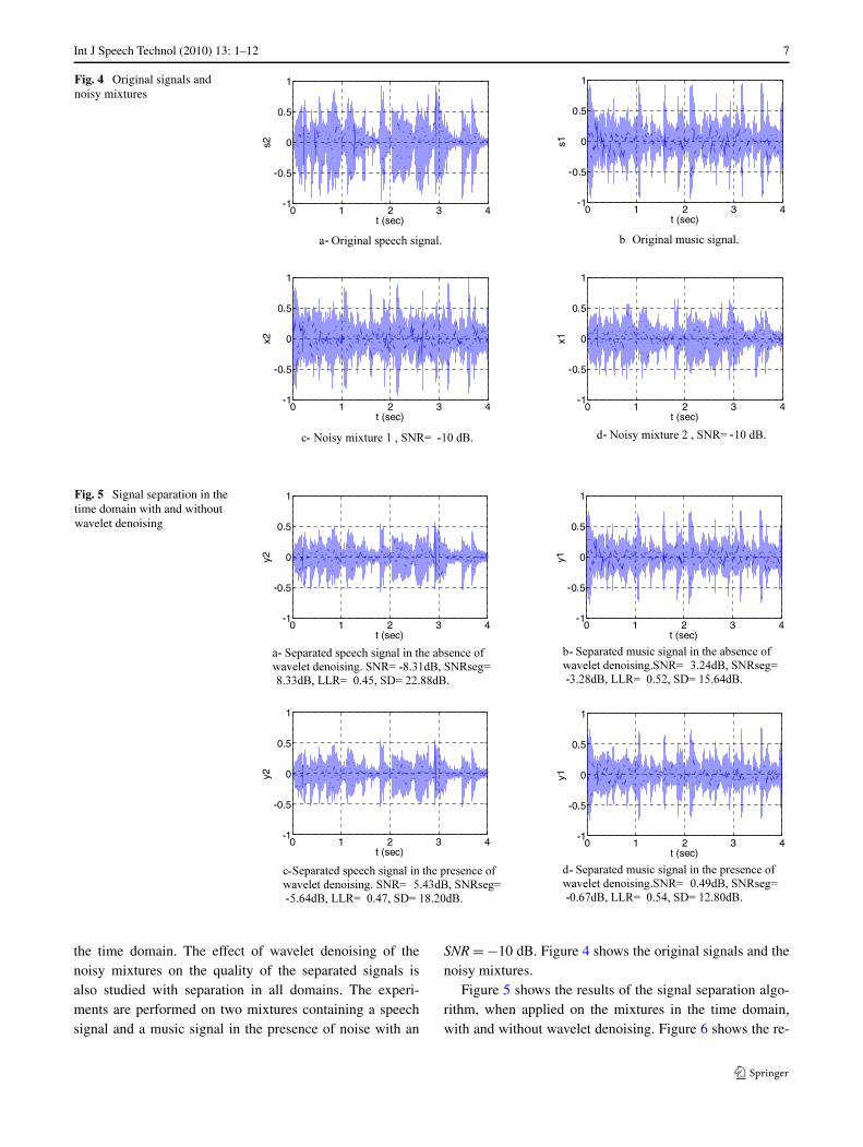
Fig. 4 Original signals andnoisy mixtures

Fig. 5 Signal separation in thetime domain with and withoutwavelet denoising

the time domain. The effect of wavelet denoising of thenoisy mixtures on the quality of the separated signals isalso studied with separation in all domains. The experi-ments are performed on two mixtures containing a speechsignal and a music signal in the presence of noise with an

SNR = −10 dB. Figure 4 shows the original signals and thenoisy mixtures.

Figure 5 shows the results of the signal separation algo-rithm, when applied on the mixtures in the time domain,with and without wavelet denoising. Figure 6 shows the re-

8 Int J Speech Technol (2010) 13: 1–12

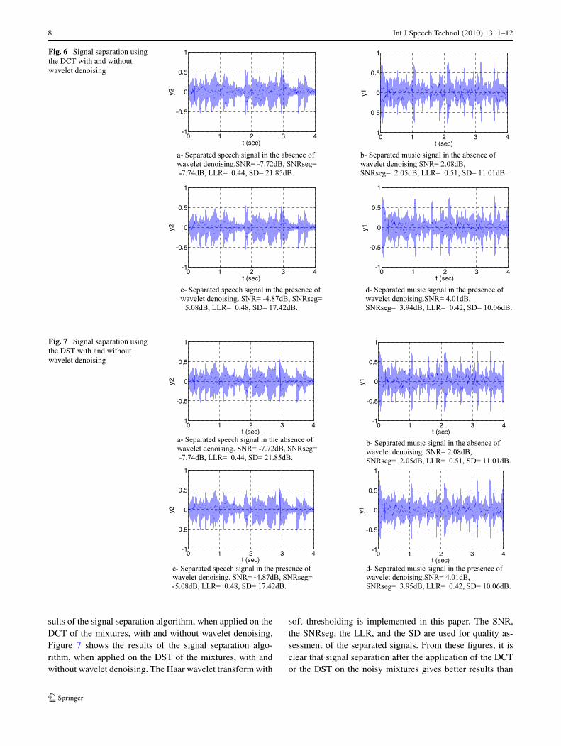
Fig. 6 Signal separation usingthe DCT with and withoutwavelet denoising

Fig. 7 Signal separation usingthe DST with and withoutwavelet denoising

sults of the signal separation algorithm, when applied on theDCT of the mixtures, with and without wavelet denoising.Figure 7 shows the results of the signal separation algo-rithm, when applied on the DST of the mixtures, with andwithout wavelet denoising. The Haar wavelet transform with

soft thresholding is implemented in this paper. The SNR,the SNRseg, the LLR, and the SD are used for quality as-sessment of the separated signals. From these figures, it isclear that signal separation after the application of the DCTor the DST on the noisy mixtures gives better results than

Int J Speech Technol (2010) 13: 1–12 9

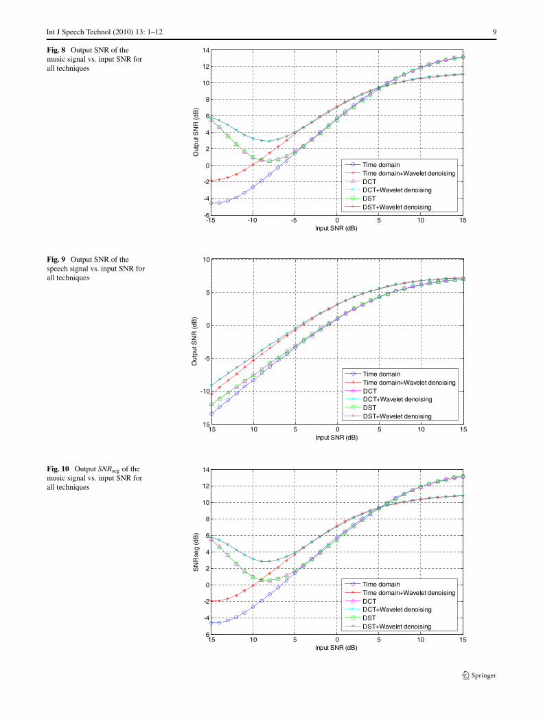
Fig. 8 Output SNR of themusic signal vs. input SNR forall techniques

Fig. 9 Output SNR of thespeech signal vs. input SNR forall techniques

Fig. 10 Output SNRseg of themusic signal vs. input SNR forall techniques

10 Int J Speech Technol (2010) 13: 1–12

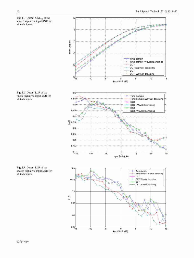
Fig. 11 Output SNRseg of thespeech signal vs. input SNR forall techniques

Fig. 12 Output LLR of themusic signal vs. input SNR forall techniques

Fig. 13 Output LLR of thespeech signal vs. input SNR forall techniques

Int J Speech Technol (2010) 13: 1–12 11

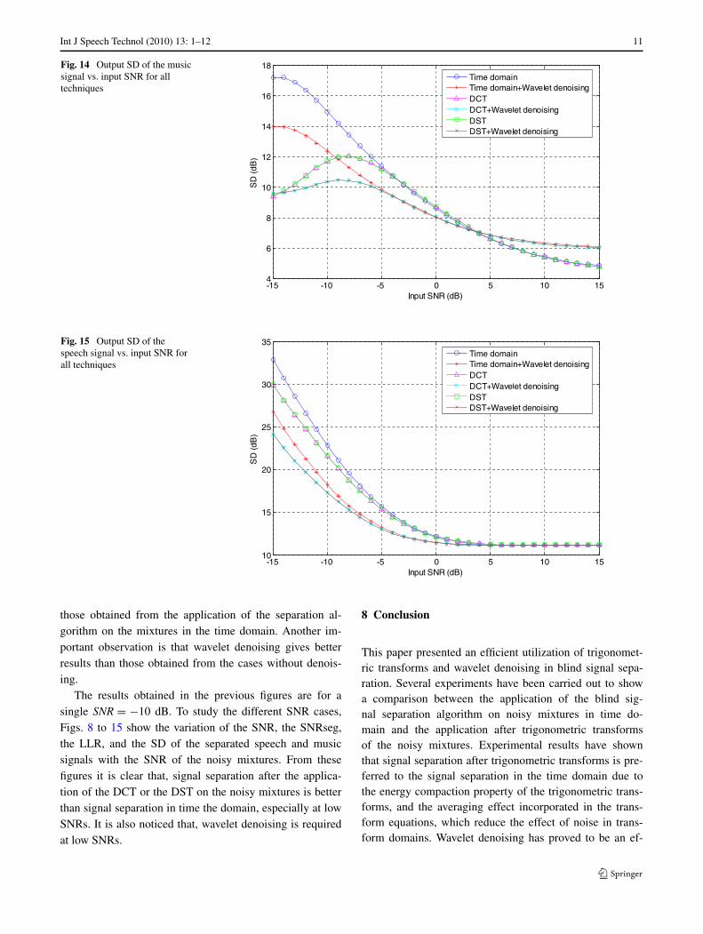
Fig. 14 Output SD of the musicsignal vs. input SNR for alltechniques

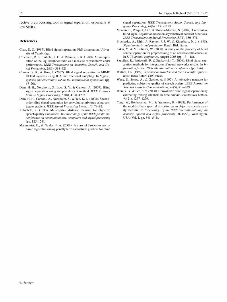
Fig. 15 Output SD of thespeech signal vs. input SNR forall techniques

those obtained from the application of the separation al-gorithm on the mixtures in the time domain. Another im-portant observation is that wavelet denoising gives betterresults than those obtained from the cases without denois-ing.

The results obtained in the previous figures are for asingle SNR = −10 dB. To study the different SNR cases,Figs. 8 to 15 show the variation of the SNR, the SNRseg,the LLR, and the SD of the separated speech and musicsignals with the SNR of the noisy mixtures. From thesefigures it is clear that, signal separation after the applica-tion of the DCT or the DST on the noisy mixtures is betterthan signal separation in time the domain, especially at lowSNRs. It is also noticed that, wavelet denoising is requiredat low SNRs.

8 Conclusion

This paper presented an efficient utilization of trigonomet-ric transforms and wavelet denoising in blind signal sepa-ration. Several experiments have been carried out to showa comparison between the application of the blind sig-nal separation algorithm on noisy mixtures in time do-main and the application after trigonometric transformsof the noisy mixtures. Experimental results have shownthat signal separation after trigonometric transforms is pre-ferred to the signal separation in the time domain due tothe energy compaction property of the trigonometric trans-forms, and the averaging effect incorporated in the trans-form equations, which reduce the effect of noise in trans-form domains. Wavelet denoising has proved to be an ef-

12 Int J Speech Technol (2010) 13: 1–12

fective preprocessing tool in signal separation, especially atlow SNRs.

References

Chan, D. C. (1997). Blind signal separation. PhD dissertation, Univer-sity of Cambridge.

Crochiere, R. E., Tribolet, J. E., & Rabiner, L. R. (1980). An interpre-tation of the log likelihood ratio as a measure of waveform coderperformance. IEEE Transactions on Acoustics, Speech, and Sig-nal Processing, 28(3), 318–323.

Curnew, S. R., & How, J. (2007). Blind signal separation in MIMOOFDM systems using ICA and fractional sampling. In Signals,systems and electronics, ISSSE’07, international symposium (pp.67–70).

Dam, H. H., Nordholm, S., Low, S. Y., & Cantoni, A. (2007). Blindsignal separation using steepest descent method. IEEE Transac-tions on Signal Processing, 55(8), 4198–4207.

Dam, H. H., Cantoni, A., Nordholm, S., & Teo, K. L. (2008). Second-order blind signal separation for convolutive mixtures using con-jugate gradient. IEEE Signal Processing Letters, 15, 79–82.

Kubichek, R. (1993). Mel-cepstral distance measure for objectivespeech quality assessment. In Proceedings of the IEEE pacific rimconference on communications, computers and signal processing(pp. 125–128).

Manmontri, U., & Naylor, P. A. (2008). A class of Frobenius norm-based algorithms using penalty term and natural gradient for blind

signal separation. IEEE Transactions Audio, Speech, and Lan-guage Processing, 16(6), 1181–1193.

Moreau, E., Pesquet, J. C., & Thirion-Moreau, N. (2007). Convolutiveblind signal separation based on asymmetrical contrast functions.IEEE Transactions on Signal Processing, 55(1), 356–371.

Prochazka, A., Uhlir, J., Rayner, P. J. W., & Kingsbury, N. J. (1998).Signal analysis and prediction. Basel: Birkhäuser.

Sakai, Y., & Mitsuhashi, W. (2008). A study on the property of blindsource separation for preprocessing of an acoustic echo cancellar.In SICE annual conference, August 2008 (pp. 13 – 18).

Szupiluk, R., Wojewnik, P., & Zabkowski, T. (2006). Blind signal sep-aration methods for integration of neural networks results. In In-formation fusion, 2006 9th international conference (pp. 1–6).

Walker, J. S. (1999). A primer on wavelets and their scientific applica-tions. Boca Raton: CRC Press.

Wang, S., Sekey, A., & Gersho, A. (1992). An objective measure forpredicting subjective quality of speech coders. IEEE Journal onSelected Areas in Communications, 10(5), 819–829.

Won, Y. G., & Lee, S. Y. (2008). Convolutive blind signal separation byestimating mixing channels in time domain. Electronics Letters,44(21), 1277–1279.

Yang, W., Benbouchta, M., & Yantorno, R. (1998). Performance ofthe modified bark spectral distortion as an objective speech qual-ity measure. In Proceedings of the IEEE international conf. onacoustic, speech and signal processing (ICASSP), Washington,USA (Vol. 1, pp. 541–544).