Blind prediction of solvation free energies from the SAMPL4challenge

David L. Mobley • Karisa L. Wymer •

Nathan M. Lim • J. Peter Guthrie

Received: 15 January 2014 / Accepted: 24 January 2014 / Published online: 11 March 2014

� Springer International Publishing Switzerland 2014

Abstract Here, we give an overview of the small mole-

cule hydration portion of the SAMPL4 challenge, which

focused on predicting hydration free energies for a series of

47 small molecules. These gas-to-water transfer free

energies have in the past proven a valuable test of a variety

of computational methods and force fields. Here, in con-

trast to some previous SAMPL challenges, we find a rel-

atively wide range of methods perform quite well on this

test set, with RMS errors in the 1.2 kcal/mol range for

several of the best performing methods. Top-performers

included a quantum mechanical approach with continuum

solvent models and functional group corrections, alchem-

ical molecular dynamics simulations with a classical all-

atom force field, and a single-conformation Poisson–

Boltzmann approach. While 1.2 kcal/mol is still a signifi-

cant error, experimental hydration free energies covered a

range of nearly 20 kcal/mol, so methods typically showed

substantial predictive power. Here, a substantial new focus

was on evaluation of error estimates, as predicting when a

computational prediction is reliable versus unreliable has

considerable practical value. We found, however, that in

many cases errors are substantially underestimated, and

that typically little effort has been invested in estimating

likely error. We believe this is an important area for further

research.

Keywords Hydration free energy � Transfer free energy �SAMPL � Free energy calculation

Introduction

Small molecule transfer free energies, and in particular

hydration free energies, have been an important topic of

research in the last few years, and have formed a portion of

every statistical assessment of modeling of proteins and

ligands (SAMPL) challenge to date [1–6]. These are

interesting in part because they are thought to provide a

proxy for the level of accuracy which could be expected for

free energy calculations in drug discovery applications, and

because they often can be calculated quite precisely, pro-

viding a quantitative test of computational methods.

Additionally, in many cases computational methods have

not been empirically adjusted to reproduce hydration free

energies, meaning that hydration free energies provide a

fair test of methods. This is especially true when new

experimental data is available, as a new set of experimental

data can be used either to assess a current method, or to

improve the method to better fit known data. The blind

challenge format we use here is designed to ensure a fair

comparison of the stated methods on new data.

Unfortunately, hydration free energies are measured

only rarely experimentally, if at all, so it is difficult to stage

a true hydration free energy prediction challenge. Typi-

cally, instead, SAMPL challenges have been based on

Electronic supplementary material The online version of thisarticle (doi:10.1007/s10822-014-9718-2) contains supplementarymaterial, which is available to authorized users.

D. L. Mobley (&) � K. L. Wymer � N. M. Lim

Departments of Pharmaceutical Sciences and Chemistry,

University of California, Irvine, 147 Bison Modular, Irvine,

CA 92697, USA

e-mail: dmobley@mobleylab.org

D. L. Mobley

Department of Chemistry, University of New Orleans,

2000 Lakeshore Drive, New Orleans, LA 70148, USA

J. P. Guthrie

Department of Chemistry, University of Western Ontario,

London, ON, Canada

123

J Comput Aided Mol Des (2014) 28:135–150

DOI 10.1007/s10822-014-9718-2

careful extraction of experimental data from obscure older

literature, where considerable expertise goes into identi-

fying relevant data, converting it to the appropriate format,

and curating it. This can include data on Henry’s law

constants, vapor pressures, solubilities, and a variety of

other sources. This SAMPL challenge is no exception, and

we are grateful to J. Peter Guthrie for his continued dedi-

cation to providing curated experimental data for the

challenge. His work for this challenge is detailed elsewhere

in this issue [7]. As in previous SAMPL challenges, the

hydration free energy component here is not truly ‘‘blind’’,

in the sense that experimental values for the compounds

can actually be extracted from the literature, but the com-

pounds examined here are typically not found in standard

hydration free energy test sets, and values are typically

difficult to extract from the primary literature. Addition-

ally, participants were asked, when submitting predictions,

to disclose any literature values consulted.

Here, our challenge involved 47 compounds selected

from a hydration free energy dataset being prepared by J.

Peter Guthrie. This set was actually divided into two por-

tions, which we called ‘‘blind’’ and ‘‘supplementary’’.

While none of the compounds were truly blind (i.e. all

experimental data used was previously published in one

form or another) the supplementary compounds were rel-

atively less obscure and values were easier to obtain from

the primary literature. In this work, we have analyzed

performance on both subsets separately, but most of our

analysis will focus on the combined set, as overall con-

clusions are qualitatively similar. Statistics for the separate

subsets are found in the Supporting Material.

In this work, we detail preparation for the SAMPL4

hydration free energy challenge, including challenge

logistics, and describe the analysis methods and metrics

used for evaluation of submissions. We also give an

overview of results from the challenge, and highlight some

of the range of methods applied. Full details of the methods

applied will be provided in reports from the individual

participants elsewhere in this issue.

SAMPL challenge preparation and logistics

The SAMPL4 challenge began with a set of 52 small

molecules represented by chemical names and SMILES

strings as provided by Guthrie [7]. From these, we gener-

ated 3D structures and isomeric SMILES strings using the

OpenEye unified Python toolkits [8]. In cases where ste-

reochemistry was not fully specified by the initial names

we were provided, stereochemistry was specified by con-

sultation with Guthrie who resolved the issue with refer-

ence to the original literature. In some cases,

stereochemistry was unimportant. Particularly, for

hydration free energy calculations, since water is an achiral

solvent, hydration free energies of enantiomers with a

single stereocenter are identical since handedness is

unimportant for the hydration free energy.1 In such cases,

one enantiomer was selected at random for the challenge.

All SAMPL participants were provided with SMILES

strings and 3D structures for all 52 compounds, and each

compound was assigned a unique identifier from

SAMPL4_001 through SAMPL4_052. Compound names

were not provided to participants prior to data submission.

Compounds with IDs through SAMPL4_021 were the

‘‘blind’’ subset, and later IDs were the ‘‘supplementary’’

subset.

The SAMPL4 challenge was advertised via the SAMPL

website (http://sampl.eyesopen.com) and e-mails to past

participants, others in the field, and the computational

chemistry list (CCL), beginning in January, 2013. The

hydration portion of the challenge was made available via

the SAMPL website February 19, 2013. Submissions for all

challenge components were due Friday, August 16, and

experimental values were provided to the participants

shortly thereafter. Statistics comparing all submissions to

experiment and to one another followed shortly thereafter.

The challenge wound up with the SAMPL4 workshop on

September 20 at Stanford University. Submissions were

allowed to be anonymous, though we received very few

anonymous submissions. Because of this, however, we

typically refer to submissions by their submission ID (a

three digit number) rather than by the authors’ names.

Method descriptions and submitter identities (from those

who were willing to share this information) are provided in

the Supporting Material.

SAMPL4 submissions involved a predicted hydration

free energy (1 M to 1M) in kcal/mol for each compound, a

predicted statistical uncertainty, and a predicted model

uncertainty. (Due to a late submission format change, a

handful of participants provided a qualitative confidence

estimate, ranging from 1 (not confident) to 5 (very confi-

dent) for each compound rather than the model uncer-

tainty). Here, we chose to distinguish between statistical

uncertainty and model uncertainty because a specific

method can often yield free energy estimates which are

very precise given the particular parameters, yet their

expected discrepancy from experiment may be substan-

tially larger than this level of precision. Our intent was that

the statistical uncertainty would represent the level of

uncertainty in the estimate given the particular model,

1 For experimental measurements, the enantiomer composition could

in principle be important if the hydration free energy is determined in

part by a solubility measurement, because the solubility of a mixture

of two enantiomers of a particular solute might be different than the

solubility of either enantiomer alone. This mainly applies to racemic

solids which form crystals with a racemic unit cell.

136 J Comput Aided Mol Des (2014) 28:135–150

123

while the model uncertainty would represent the level of

uncertainty expected due to the details of the model. For

example, a set of alchemical molecular dynamics simula-

tions based on AM1-BCC and GAFF might yield hydration

free energies to a precision of 0.2 kcal/mol (so that other

participants using the same approach and simulation

parameters, but different starting conditions or simulation

packages, might see a typical variance of 0.2 kcal/mol) but

the expected error relative to experiment could be sub-

stantially higher, perhaps 1.4 kcal/mol [9]. Similarly, for

single-conformation methods, the statistical uncertainty

might reflect variations in the selected solute conformation

and other factors, while the model uncertainty would reflect

expected error relative to experiment. Ideally a given

approach would accurately quantify both of these uncer-

tainties—the level of reproducibility given the overall

approach, and the level of expected error relative to

experiment.

After the challenge was launched, problems with

experimental values, SMILES strings, or structures for a

number of compounds were uncovered, resulting in

removal of some five compounds from the challenge. Most

of these removals occurred prior to the SAMPL meeting,

and were reflected in the analysis provided to participants

prior to the meeting. Specifically, SAMPL4_040, 018, and

031 were removed because they were not the intended

compounds. However, investigation around and after the

SAMPL meeting of several problematic members of the

guaiacol series resulted in removal of 4,5-dichloroguaiacol

(SAMPL4_007) and and 5-chloroguaiacol (SAMPL4_008)

on October 24. Additional, values of SAMPL4_006 (4-

propyl-guaiacol), 024 (ami-triptyline), 013 (carveol), 012

(dihydrocarvone), 016 (menthol), 017 (menthone), and 015

(piperitone) were revised slightly at that time based on a re-

analysis of the experimental data, though the only com-

pound for which the value changed more than the experi-

mental uncertainty was 4-propylguaiacol. These changes

brought essentially every method into better agreement

with experiment, but did not appear to substantially affect

the overall rank-ordering of the performance of different

submissions. The value of SAMPL4_021, 1-benzylimida-

zole, was also corrected post-SAMPL (September 10) after

a mistake was identified in a table reporting the original

experimental data, and the authors provided a correction

[7].

In some past SAMPLs, specific functional groups or

classes of molecules have proven particularly challenging.

In an anticipation that this might also be true here, we

conceptually divided the set into five groups. Group 1

consists of linear or branched alkanes or alkenes with

various polar functional groups. Group 2 consists of

methoxyphenol and guaiacol, chlorinated derivatives, and

other rather similar compounds. Group 3 consists of

cyclohexane derivatives, often also with an attached oxy-

gen or hydroxyl. Group 4 consists of anthracene deriva-

tives, many of which have attached polar functional

groups. And group 5 is polyfunctional or other compounds,

and contains the largest and most flexible compounds in the

set.

Several of the submissions discussed here came from the

Mobley lab. Specifically, submission IDs 004, 005, 014,

and 015 were run internally in the Mobley lab. 004 and 005

were run by KLW, an undergraduate student in the lab,

who had no involvement in other portions of the hydration

challenge setup or analysis. These predictions were done

prior to the SAMPL submission deadline, and their blind

nature means they were done on equal footing with any of

the SAMPL submissions, despite the fact that they were

conducted in the lab coordinating this aspect of the chal-

lenge. In contrast, 014 and 015 are null or comparison

models run after the SAMPL challenge by DLM and KLW,

and were done knowing (but not utilizing) the results of the

challenge.

Submissions IDs 014 and 015 were included out of a

desire to include a simplistic knowledge-based model for

comparison with the more physical approaches employed

by most participants. Both approaches compared each

SAMPL challenge compound to a database of 640 small

molecules studied previously by the Mobley lab including

those from all previous SAMPLs [3–6, 9, 10]. For each

compound in this SAMPL, the submission assigned a

‘‘predicted’’ value equal to the experimental value of the

most similar compound (submission 014) or the average of

the three most similar compounds (submission 015).

Chemical similarities were assigned based on OpenEye’s

Shape ? color score. Thus, this provided a crude knowl-

edge-based approach simply based on chemical similarity.

SAMPL analysis methods

Analysis metrics

SAMPL analysis was conducted via Python script, using

NumPy and SciPy for numerics and Matplotlib for plots.

All submissions were analyzed by a variety of standard

metrics, including average error, average unsigned error,

RMS error, Pearson correlation coefficient (R), and Ken-

dall tau, as well as the slope of a best linear fit of calculated

to predicted values, the ‘‘error slope’’, explained below. We

also looked at the largest error each method makes, by

compound, to get a better sense of overall reliability.

Furthermore, we computed the Kendall W, discussed

below. Additionally, we compared the median Kullback–

Leibler (KL) divergence for all methods, adjusted to avoid

penalizing for predicted uncertainties that are smaller than

J Comput Aided Mol Des (2014) 28:135–150 137

123

the experimental error when the calculated value is close to

the experimental value, as we explain further below.

Because KL divergences are difficult to average when

performance is poor, we also looked at the expected loss, L,

given by

L ¼ h1� e�KLi ð1Þ

where KL is the KL divergence for an individual predic-

tion, and the average runs over all predictions within a

submission.

KL divergence

Our interest in KL divergence here was motivated partly by

the realization that even an unreliable computational method

could, in the right hands, be extremely useful as long as one

can predict when it will be unreliable. Or, to put it another

way, an ideal metric for evaluating methods would:

1. Maximally reward only predictions which are high

confidence, high accuracy

2. Provide only a small reward to predictions which are

low confidence, high accuracy

3. Provide only a small penalty to predictions which are

low confidence, low accuracy

4. Maximally penalize only predictions which are high

confidence, low accuracy

5. Recognize experimental measurements have error, and

incorporate experimental uncertainties

6. Neither penalize nor reward predictions for being more

precise than the experimental point of comparison, if

they are consistent with it

On item 6, we can imagine a hypothetical computational

method which could produce extremely accurate and precise

predictions, with even greater precision than experiment.

While we could not fully validate such predictions, there

should be no penalty for methods which are more precise

than experiment (but neither should there be any reward).

KL divergence is given by:

KL ¼Z

p lnp

qdu ð2Þ

where p and q are the two distributions being compared

(here, p represents the distribution of experimental values

and q the distribution of calculated values). It is zero only if

the two distributions are identical, and infinite when they

have no overlap. If both the experimental and calculated

distributions are modeled as Gaussians, as here, the

expression simplifies further [2].

The KL divergence method was employed in a previous

SAMPL because it has a number of the right properties [2].

Specifically, it essentially covers points 1–5. Both experi-

mental and calculated values are modeled by distributions,

and are rewarded for overlap, with overlap increasing both

by increasingly accurate predictions, and (at least for pre-

dictions disagreeing with experimental values) improving

uncertainty estimates.

Unfortunately, without further modification, KL diver-

gence fails at handling item 6. Specifically, predicted values

with uncertainty estimates smaller than the experimental

uncertainty are penalized—effectively, the ideal method,

within this framework, would be as precise as the experi-

mental measurements but no more precise. This is prob-

lematic, so a first-order fix is to use the experimental error as

the predicted error in all cases [2]. While this prevents

unfairly penalizing precise computational methods, it also

removes the penalty warranted by item 4—high precision,

low accuracy predictions are no longer penalized more than

low precision, low accuracy predictions. Wood et al. alter-

natively addressed this problem by replacing the predicted

error with the experimental error whenever the predicted

error is smaller than the experimental error. Unfortunately,

this too reduces the penalty for methods which are more

precise than the experiment but substantially wrong 1.

We believe, if the KL divergence is to be employed as a

metric, the correct approach is to smoothly transition

between two limits. In one limit, when the experimental

value and the prediction fundamentally agree, predictions

should not be penalized for being more precise than

experiment, and so if the predicted uncertainty is smaller

than the experimental uncertainty, it should be made to

match, for optimal overlap (minimal divergence). In the

other limit, where the predicted and experimental values

completely disagree, the original predicted uncertainty

estimate should be retained. Thus, if two substantially

incorrect predictions which are the same are compared to

experiment, the one with the larger uncertainty estimate

will always result in a better KL divergence. We would like

to transition smoothly between these two limits.

Thus, here our approach for computing the KL diver-

gence is to model the experimental value and the prediction

as Gaussian distributions. The experimental distribution

always has a variance re, the experimental uncertainty.

And the predicted distribution has a variance of

max(rp, r0p), where rp is the original uncertainty estimate

for the prediction, r0p = f 9 re ? (1 - f) 9 rp, and f is a

mixing factor given by either:

f ¼ expð�jDlj=rcÞ ð3Þ

or

f ¼ expð�ðDl=rcÞ2Þ ð4Þ

138 J Comput Aided Mol Des (2014) 28:135–150

123

where rc = re2 ? rp

2 is the mutual uncertainty, and Dl ¼le � lc is the difference between the predicted and

experimental values (or the means of the predicted and

experimental distributions). We call these the exponential

and Gaussian mixing schemes, respectively. In either case,

f = 0 when the calculated and experimental values are far

separated, so that r0p = rp, and f = 1 when the predicted

and experimental mean are identical, so that r0p = re. This

results in substantial changes in the KL divergence relative

to alternative approaches, as we highlight in Fig. 1. Here,

while we see significant differences between KL diver-

gences obtained via Eqs. 3 and 4 in a few cases, we are not

aware of a strong reason to prefer one approach over the

other so we use the simpler scheme, Eq. 3 (Fig. 1).

There is one additional nuance here, in that submis-

sions actually provided two uncertainty estimates—the

statistical uncertainty and the model uncertainty. Ideally,

we would have made it very clear to participants in

advance how we intended to use these, but as our plans

came together after we began analyzing submissions, we

were unable to do so. Ideally, we would have made it

clear that ‘‘model uncertainty’’ estimates would be used

to assess how well participants did at estimating how

well their methods would agree with experiment, on

each compound. But since this was not sufficiently clear,

for KL divergence, we used the larger of the two

uncertainty estimates submitted, which in general

resulted in more favorable KL divergences than alter-

native approaches.

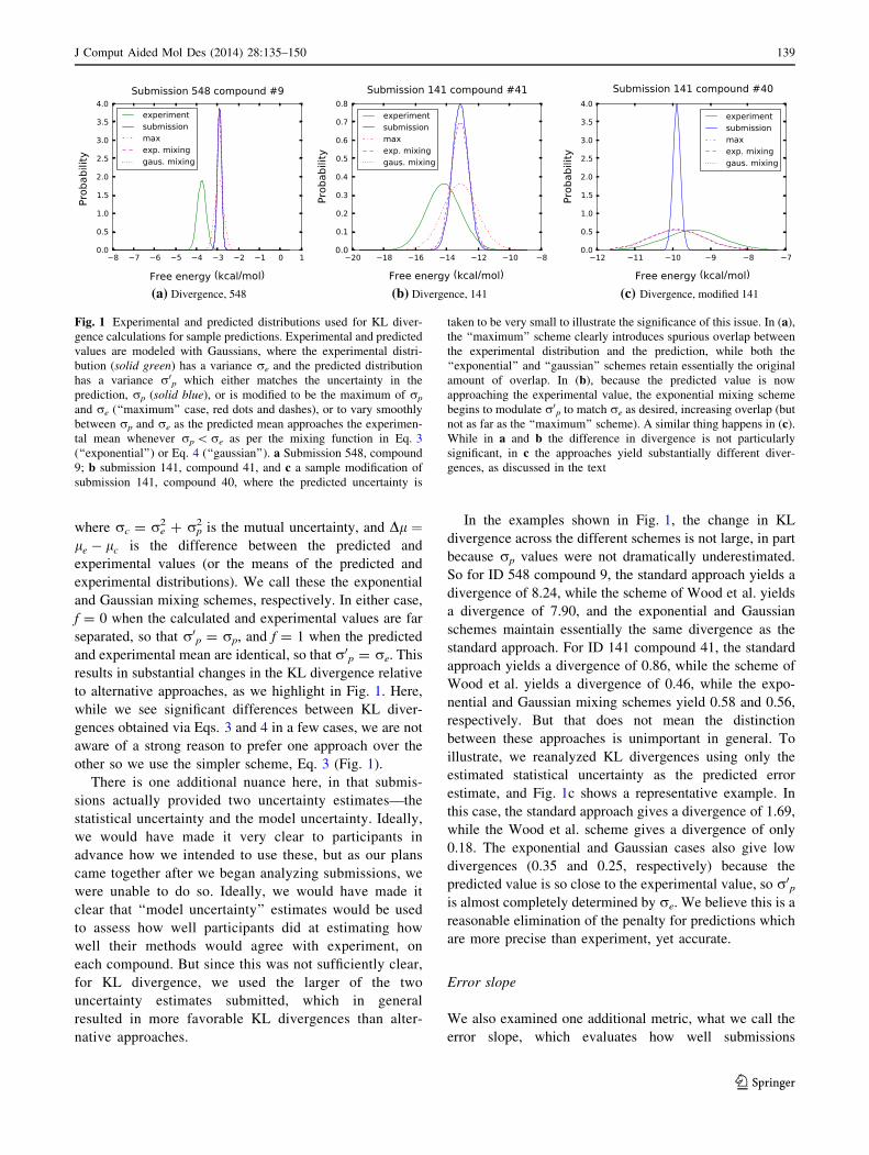
In the examples shown in Fig. 1, the change in KL

divergence across the different schemes is not large, in part

because rp values were not dramatically underestimated.

So for ID 548 compound 9, the standard approach yields a

divergence of 8.24, while the scheme of Wood et al. yields

a divergence of 7.90, and the exponential and Gaussian

schemes maintain essentially the same divergence as the

standard approach. For ID 141 compound 41, the standard

approach yields a divergence of 0.86, while the scheme of

Wood et al. yields a divergence of 0.46, while the expo-

nential and Gaussian mixing schemes yield 0.58 and 0.56,

respectively. But that does not mean the distinction

between these approaches is unimportant in general. To

illustrate, we reanalyzed KL divergences using only the

estimated statistical uncertainty as the predicted error

estimate, and Fig. 1c shows a representative example. In

this case, the standard approach gives a divergence of 1.69,

while the Wood et al. scheme gives a divergence of only

0.18. The exponential and Gaussian cases also give low

divergences (0.35 and 0.25, respectively) because the

predicted value is so close to the experimental value, so r0pis almost completely determined by re. We believe this is a

reasonable elimination of the penalty for predictions which

are more precise than experiment, yet accurate.

Error slope

We also examined one additional metric, what we call the

error slope, which evaluates how well submissions

(a) Divergence, 548 (b) Divergence, 141 (c) Divergence, modified 141

Fig. 1 Experimental and predicted distributions used for KL diver-

gence calculations for sample predictions. Experimental and predicted

values are modeled with Gaussians, where the experimental distri-

bution (solid green) has a variance re and the predicted distribution

has a variance r0p which either matches the uncertainty in the

prediction, rp (solid blue), or is modified to be the maximum of rp

and re (‘‘maximum’’ case, red dots and dashes), or to vary smoothly

between rp and re as the predicted mean approaches the experimen-

tal mean whenever rp \re as per the mixing function in Eq. 3

(‘‘exponential’’) or Eq. 4 (‘‘gaussian’’). a Submission 548, compound

9; b submission 141, compound 41, and c a sample modification of

submission 141, compound 40, where the predicted uncertainty is

taken to be very small to illustrate the significance of this issue. In (a),

the ‘‘maximum’’ scheme clearly introduces spurious overlap between

the experimental distribution and the prediction, while both the

‘‘exponential’’ and ‘‘gaussian’’ schemes retain essentially the original

amount of overlap. In (b), because the predicted value is now

approaching the experimental value, the exponential mixing scheme

begins to modulate r0p to match re as desired, increasing overlap (but

not as far as the ‘‘maximum’’ scheme). A similar thing happens in (c).

While in a and b the difference in divergence is not particularly

significant, in c the approaches yield substantially different diver-

gences, as discussed in the text

J Comput Aided Mol Des (2014) 28:135–150 139

123

predicted uncertainties. This begins by looking at the

fraction of experimental values (resampled with noise

drawn from the experimental distribution) falling within a

given multiple of a submissions assigned statistical

uncertainty, and compares it to the fraction expected

graphically. This initial plot is effectively a Q–Q plot,

comparing the expected number of values within a partic-

ular quantile with the actual number within a particular

quantile. A similar approach was used previously by

Chodera and Noe to validate computed uncertainty esti-

mates [11]. Here, however, we seek a numerical metric for

the quality of uncertainty estimates, so we perform a linear

least-squares fit to our Q–Q plot, with the intercept con-

strained to be zero. This gives us the slope of the best fit

line which best relates the observed fraction of experi-

mental values within a given number of quantiles of the

calculated value to the expected fraction within the same

range, as shown in Fig. 2. A slope of 1 corresponds to

uncertainty estimates which are accurate on average, while

a slope larger or smaller than 1 corresponds to uncertainty

estimates which are on average too high or too low

respectively, so the target value here is 1. We call this

value the ‘‘error slope’’ for brevity.

Again, because we had not made our plans for han-

dling of statistical uncertainty and model uncertainty

sufficiently clear to participants, we had to be careful how

to handle the two uncertainty estimates as they pertained

to error slope. Our final solution was to compute the error

slope both for the statistical uncertainty, and the model

uncertainty, and report the slope value which was closer

to 1. Effectively, we gave participants credit for which-

ever error estimate was the more reasonable of the two

they submitted.

Kendall W

Here, we also applied the Kendall W statistic to assess the

level of agreement about which submission or method

performed best overall. Kendall W ranges from 0 to 1, and

assesses the degree of consistency between evaluations,

with 0 representing complete disagreement and 1 repre-

senting complete agreement. For example, a group of

judges might rank a series of wines, and a W value of 1

would correspond to complete agreement between judges

about which wine was best, while a W value of zero would

correspond to complete disagreement. Here, each com-

pound effectively serves as a judge, and we evaluate sub-

missions based on their ranked performance on different

compounds. A Kendall W value of 1 would mean that a

single method was the top performer across all compounds,

while a value not significantly different from 0 would mean

no method was a clear leader across all compounds.

Error analysis

In addition to calculating various metrics comparing per-

formance, we computed uncertainties in these values using

a bootstrapping procedure accounting for experimental

noise. Specifically, for every set of predicted values, we

conducted 1000 bootstrap trials, and our uncertainty esti-

mate was taken as the variance in each metric computed

across those trials. Each bootstrap trial consisted of con-

structing a new set of calculated and experimental values

(of the same length) by selecting compounds from the

original set, with replacement. In each bootstrap trial, noise

was added independently to each experimental value with a

value drawn from a Gaussian distribution with a mean of

zero and a variance equal to the experimental uncertainty.

Thus bootstrapped error estimates effectively include both

variation due to the composition of the set, and due to the

experimental uncertainties themselves.

Significance testing

In some cases we sought to compare whether methods with

marginally different performance are actually significantly

different, or in other words we seek to determine whether

our data (the comparison of predicted with experimental

values for two different methods) is enough to reject the

null hypothesis that two methods being compared are in

fact no different. To do this, we here applied Student’s

paired t test [12] to the difference between the calculated

and experimental values for the sets being compared. This

allowed us to test whether methods yielded predictions

which were substantially different—predictions drawn

from significantly different distributions. This test does not

indicate whether one method is superior to another, but

simply whether their predictions are different in a signifi-

cant way. This allows us, among other things, to compare

whether two top-performing methods are different in a

statistically significant way, or whether a given method

yields predictions which are different in a significant way

from a control model such as a similarity-based model

(submission 014 or 015).

Results and discussion

Performance statistics

The SAMPL4 hydration challenge involved 49 submis-

sions from 19 groups. As in past SAMPLs, many groups

submitted multiple sets of predictions to test and cross-

compare diverse methods. Overall, we ran the full range of

statistics on all submissions, and results on the full set are

shown in Table 1. To allow graphical comparison of

140 J Comput Aided Mol Des (2014) 28:135–150

123

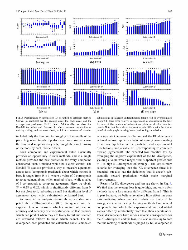
methods, we also ranked all submissions by each metric we

examined and provide the same statistics in bar graph form

in Fig. 3. It is worth highlighting that uncertainties are

substantial, and in many cases larger than the difference

between submissions, so while submissions can be ranked

by these metrics, the precise order of the ranking would be

subject to statistical fluctuations if the set were modified or

even if experiments were repeated. Qualitatively, this can

be seen graphically from the figures by looking at the level

of overlap between error bars.

One participant (five submissions) focused exclusively

on the blind component of the challenge, and thus statistics

for these submissions could not be computed for the full

set. Separate tables showing performance on the blind and

supplementary portions of the challenge are provided in the

Supporting Information. Submissions 530–534, which

(a) Performance, 561 (b) Performance, 567

(c) Error estimation, 561 (d) Error estimation, 567

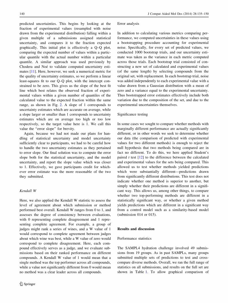
Fig. 2 Overall performance and error estimation performance for

submissions ID 561 and 567. The top plots show the overall

performance at prediction hydration free energies for two represen-

tative submissions. Superficially, performance looks similar. How-

ever, in the top right panel, one compound has an extremely large

error, and far more compounds are not within the predicted

uncertainty of the experimental value. In other words, submission

ID 567 underestimated uncertainties. This is supported by examining

Q–Q plots (bottom) looking at the fraction of experimental values

falling within a given range of the predicted value versus the expected

fraction. The black line shows x = y, expected if uncertainty

estimates are on average correct, and purple is the best-fit line with

intercept 0; we call the slope of this line the error slope. Overall,

submission 561 appears to overestimate uncertainties (slope 1.23 [1)

while submission 567 substantially underestimates uncertainties

(slope 0.62 \1)

J Comput Aided Mol Des (2014) 28:135–150 141

123

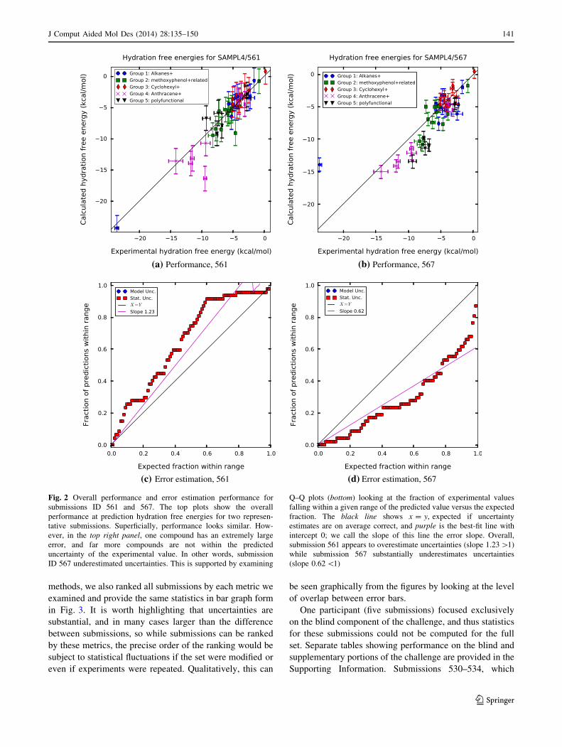
Table 1 Statistics for SAMPL4 hydration prediction

ID Avg. err. RMS AUE tau R Err. slope Max. err.

004 0.13 ± 0.13 1.40 ± 0.12 1.10 ± 0.10 0.73 ± 0.06 0.93 ± 0.02 0.99 ± 0.07 4.98 ± 0.47

005 -0.42 ± 0.18 1.22 ± 0.15 0.96 ± 0.12 0.78 ± 0.06 0.96 ± 0.01 1.06 ± 0.05 1.81 ± 0.67

014 1.11 ± 0.57 3.07 ± 0.72 1.90 ± 0.51 0.36 ± 0.15 0.71 ± 0.26 1.01 ± 0.10 10.69 ± 0.70

015 1.02 ± 0.49 3.09 ± 0.46 2.02 ± 0.34 0.36 ± 0.09 0.65 ± 0.20 1.00 ± 0.07 10.37 ± 0.42

137 2.24 ± 0.23 2.89 ± 0.30 2.48 ± 0.20 0.70 ± 0.06 0.89 ± 0.03 0.70 ± 0.08 8.38 ± 0.50

138 0.51 ± 0.29 2.00 ± 0.23 1.66 ± 0.20 0.65 ± 0.06 0.90 ± 0.05 0.57 ± 0.08 5.25 ± 0.23

141 -0.07 ± 0.28 1.46 ± 0.18 1.07 ± 0.11 0.74 ± 0.07 0.93 ± 0.02 0.72 ± 0.08 6.02 ± 0.46

145 -0.44 ± 0.16 1.23 ± 0.16 0.87 ± 0.09 0.81 ± 0.03 0.98 ± 0.01 0.86 ± 0.08 1.24 ± 0.89

149 0.03 ± 0.24 1.46 ± 0.14 1.12 ± 0.12 0.73 ± 0.05 0.94 ± 0.02 0.55 ± 0.04 2.74 ± 0.89

152 -3.48 ± 0.98 5.52 ± 1.25 4.05 ± 0.85 0.39 ± 0.08 0.57 ± 0.17 0.31 ± 0.06 3.93 ± 3.84

153 -2.35 ± 0.52 3.95 ± 0.40 3.07 ± 0.41 0.49 ± 0.04 0.75 ± 0.10 0.57 ± 0.06 2.95 ± 0.77

158 0.55 ± 1.76 10.14 ± 1.91 7.23 ± 1.09 0.63 ± 0.05 0.48 ± 0.08 0.09 ± 0.02 9.29 ± 6.10

166 -0.38 ± 0.22 1.58 ± 0.09 1.24 ± 0.08 0.70 ± 0.05 0.92 ± 0.05 1.28 ± 0.03 3.55 ± 0.33

167 -0.41 ± 0.52 4.48 ± 1.20 2.15 ± 0.61 0.49 ± 0.12 0.57 ± 0.14 1.20 ± 0.08 4.94 ± 3.18

168 -0.42 ± 0.89 4.53 ± 1.49 2.22 ± 0.72 0.49 ± 0.11 0.56 ± 0.17 1.18 ± 0.08 4.91 ± 5.36

169 -0.53 ± 0.29 2.32 ± 0.32 1.75 ± 0.24 0.51 ± 0.10 0.83 ± 0.07 1.15 ± 0.06 4.26 ± 1.42

178 0.25 ± 0.17 1.52 ± 0.11 1.28 ± 0.11 0.71 ± 0.05 0.93 ± 0.02 1.32 ± 0.03 3.42 ± 0.16

179 0.24 ± 0.29 1.55 ± 0.20 1.23 ± 0.16 0.68 ± 0.07 0.92 ± 0.02 1.27 ± 0.04 4.42 ± 0.39

180 -0.73 ± 0.18 1.96 ± 0.24 1.54 ± 0.17 0.66 ± 0.07 0.94 ± 0.03 1.32 ± 0.04 2.36 ± 0.86

181 -0.49 ± 0.23 1.55 ± 0.13 1.24 ± 0.12 0.69 ± 0.08 0.94 ± 0.04 1.31 ± 0.04 3.19 ± 0.74

189 0.28 ± 0.39 2.74 ± 0.43 1.95 ± 0.28 0.49 ± 0.11 0.76 ± 0.14 1.13 ± 0.06 8.72 ± 1.33

196 0.78 ± 1.36 9.88 ± 1.89 7.17 ± 1.19 0.64 ± 0.03 0.44 ± 0.08 0.11 ± 0.01 9.29 ± 8.23

197 0.87 ± 0.97 10.60 ± 1.15 7.74 ± 0.68 0.62 ± 0.05 0.38 ± 0.07 0.04 ± 0.01 10.29 ± 2.07

529 0.26 ± 0.30 2.39 ± 0.34 1.82 ± 0.25 0.60 ± 0.07 0.85 ± 0.05 1.13 ± 0.05 6.83 ± 0.69

542 -0.10 ± 0.29 1.89 ± 0.26 1.30 ± 0.18 0.64 ± 0.07 0.90 ± 0.07 1.04 ± 0.04 5.24 ± 0.26

543 0.35 ± 0.18 1.80 ± 0.22 1.35 ± 0.15 0.64 ± 0.05 0.90 ± 0.06 0.98 ± 0.04 5.44 ± 0.92

544 0.37 ± 0.18 1.26 ± 0.15 1.00 ± 0.09 0.77 ± 0.03 0.95 ± 0.01 1.12 ± 0.04 4.22 ± 0.20

545 1.04 ± 0.25 2.96 ± 0.28 2.32 ± 0.21 0.47 ± 0.11 0.73 ± 0.13 0.64 ± 0.07 8.02 ± 1.73

548 1.29 ± 0.31 2.80 ± 0.49 2.08 ± 0.31 0.54 ± 0.11 0.83 ± 0.13 0.57 ± 0.07 9.22 ± 0.91

561 -0.22 ± 0.26 1.58 ± 0.34 1.08 ± 0.19 0.77 ± 0.03 0.94 ± 0.02 1.23 ± 0.04 2.60 ± 1.47

562 0.67 ± 0.21 1.68 ± 0.13 1.45 ± 0.13 0.73 ± 0.06 0.92 ± 0.02 1.01 ± 0.06 3.66 ± 0.60

563 -0.16 ± 0.26 2.49 ± 0.28 1.87 ± 0.23 0.50 ± 0.09 0.78 ± 0.03 0.95 ± 0.09 7.30 ± 0.40

564 0.26 ± 0.29 2.82 ± 0.34 2.21 ± 0.25 0.43 ± 0.11 0.77 ± 0.08 0.85 ± 0.04 8.66 ± 1.14

565 0.48 ± 0.17 1.30 ± 0.20 0.98 ± 0.15 0.77 ± 0.04 0.95 ± 0.02 0.93 ± 0.05 4.34 ± 0.47

566 0.34 ± 0.14 1.23 ± 0.16 0.94 ± 0.11 0.78 ± 0.04 0.95 ± 0.01 0.95 ± 0.07 4.22 ± 0.25

567 -0.69 ± 0.21 2.34 ± 0.32 1.72 ± 0.19 0.63 ± 0.05 0.83 ± 0.04 0.62 ± 0.09 9.72 ± 0.61

568 -0.87 ± 0.18 1.56 ± 0.11 1.21 ± 0.11 0.76 ± 0.05 0.94 ± 0.02 0.83 ± 0.05 2.72 ± 0.15

569 -2.97 ± 0.59 4.34 ± 0.60 3.25 ± 0.50 0.55 ± 0.05 0.77 ± 0.05 0.41 ± 0.06 4.12 ± 2.05

570 -2.48 ± 0.33 3.27 ± 0.41 2.53 ± 0.31 0.72 ± 0.05 0.88 ± 0.04 0.36 ± 0.05 0.55 ± 0.57

572 -0.68 ± 0.18 2.24 ± 0.32 1.64 ± 0.22 0.63 ± 0.09 0.84 ± 0.03 0.66 ± 0.07 9.12 ± 0.24

573 -0.85 ± 0.16 1.46 ± 0.13 1.15 ± 0.12 0.78 ± 0.06 0.95 ± 0.03 0.83 ± 0.07 1.92 ± 0.54

575 -0.81 ± 0.25 2.11 ± 0.35 1.59 ± 0.19 0.67 ± 0.09 0.89 ± 0.05 0.60 ± 0.07 3.16 ± 1.33

582 0.27 ± 1.01 4.50 ± 0.79 3.25 ± 0.59 0.67 ± 0.11 0.84 ± 0.05 0.55 ± 0.09 8.50 ± 2.49

Shown are statistics for each submission, by submission ID. We report average error, RMS error, average unsigned error, Kendall tau, Pearson R,

the slope of a best fit line comparing predicted error with actual error (with an ideal value of 1, as described in the text), and the maximum error

on any individual compound. Units, when applicable, are kcal/mol. Submission 575 was apparently affected with a propagation bug when

running the molecular dynamics simulations, introducing errors [13]

142 J Comput Aided Mol Des (2014) 28:135–150

123

included only the blind set, fall roughly in the middle of the

pack. In general, trends in performance were similar across

the blind and supplementary sets, though the exact ranking

of methods by each metric differs.

Each compound and experimental value essentially

provides an opportunity to rank methods, and if a single

method provided the best prediction for every compound

considered, such a method would be a clear winner. The

Kendall W statistic provides a way to measure agreement

across tests (compounds predicted) about which method is

best. It ranges from 0 to 1, where a value of 0 corresponds

to no agreement about which method is best, while a value

of 1 corresponds to complete agreement. Here, we obtain

W = 0.28 ± 0.02, which is significantly different from 0,

but not close to 1, indicating a small but significant level of

agreement about which submissions performed best.

As noted in the analysis section above, we also com-

puted the Kullback–Leibler (KL) divergence and the

expected loss as measures which combine both method

accuracy and accuracy of error estimation, so that methods

which can predict when they are likely to fail and succeed

are rewarded relative to those which cannot. For KL

divergence, each predicted and calculated value is modeled

as a separate Gaussian distribution and the KL divergence

is based on overlap, with a value of infinity corresponding

to no overlap between the predicted and experimental

distributions, and a value of 0 corresponding to complete

overlap (agreement). The expected loss modifies this by

averaging the negative exponential of the KL divergence,

yielding a value which ranges from 0 (perfect predictions)

to 1 (a high KL divergence on average). The loss is more

suitable for averaging than the KL divergence since it is

bounded, but also has the deficiency that it doesn’t sub-

stantially reward predictions which make marginal

improvements.

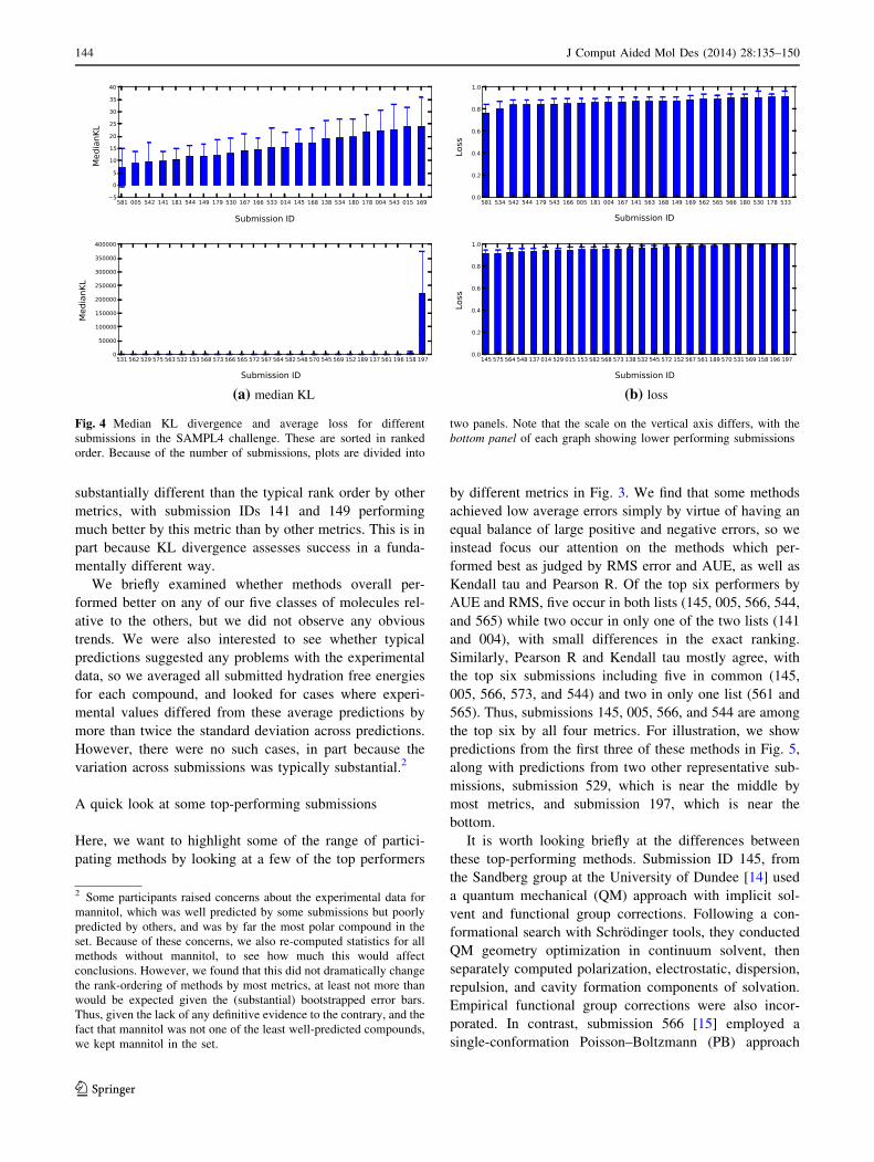
Results for KL divergence and loss are shown in Fig. 4.

We find that the average loss is quite high, and only a few

methods have a loss substantially different from 1. This is

in part because, we believe, relatively little effort has gone

into predicting when predicted values are likely to be

wrong, so even the best performing methods have several

compounds for which the experimental and calculated

values differ by substantially more than their uncertainties.

These discrepancies have serious adverse consequences for

the KL divergence and the loss. It is also interesting to note

that the ranking of methods as judged by KL divergence is

(a) avg. err (b) RMS (c) AUE

(d) tau (e) R (f) err. slope

Fig. 3 Performance by submission ID, as ranked by different metrics.

Shown (in kcal/mol) are the average error, the RMS error, and the

average unsigned error (AUE) (a–c). Additionally, we show the

Kendall tau value and Pearson R, which measure correlation or

ranking ability, and the error slope, which is a measure of whether

submissions on average underestimated (slope \1) or overestimated

(slope[1) their error relative to experiment, as discussed in the text.

Because of the number of submissions, plots are divided into two

panels. Note that the scale on the vertical axis differs, with the bottom

panel of each graph showing lower performing submissions

J Comput Aided Mol Des (2014) 28:135–150 143

123

substantially different than the typical rank order by other

metrics, with submission IDs 141 and 149 performing

much better by this metric than by other metrics. This is in

part because KL divergence assesses success in a funda-

mentally different way.

We briefly examined whether methods overall per-

formed better on any of our five classes of molecules rel-

ative to the others, but we did not observe any obvious

trends. We were also interested to see whether typical

predictions suggested any problems with the experimental

data, so we averaged all submitted hydration free energies

for each compound, and looked for cases where experi-

mental values differed from these average predictions by

more than twice the standard deviation across predictions.

However, there were no such cases, in part because the

variation across submissions was typically substantial.2

A quick look at some top-performing submissions

Here, we want to highlight some of the range of partici-

pating methods by looking at a few of the top performers

by different metrics in Fig. 3. We find that some methods

achieved low average errors simply by virtue of having an

equal balance of large positive and negative errors, so we

instead focus our attention on the methods which per-

formed best as judged by RMS error and AUE, as well as

Kendall tau and Pearson R. Of the top six performers by

AUE and RMS, five occur in both lists (145, 005, 566, 544,

and 565) while two occur in only one of the two lists (141

and 004), with small differences in the exact ranking.

Similarly, Pearson R and Kendall tau mostly agree, with

the top six submissions including five in common (145,

005, 566, 573, and 544) and two in only one list (561 and

565). Thus, submissions 145, 005, 566, and 544 are among

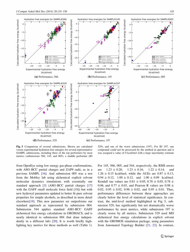
the top six by all four metrics. For illustration, we show

predictions from the first three of these methods in Fig. 5,

along with predictions from two other representative sub-

missions, submission 529, which is near the middle by

most metrics, and submission 197, which is near the

bottom.

It is worth looking briefly at the differences between

these top-performing methods. Submission ID 145, from

the Sandberg group at the University of Dundee [14] used

a quantum mechanical (QM) approach with implicit sol-

vent and functional group corrections. Following a con-

formational search with Schrodinger tools, they conducted

QM geometry optimization in continuum solvent, then

separately computed polarization, electrostatic, dispersion,

repulsion, and cavity formation components of solvation.

Empirical functional group corrections were also incor-

porated. In contrast, submission 566 [15] employed a

single-conformation Poisson–Boltzmann (PB) approach

(a) median KL (b) loss

Fig. 4 Median KL divergence and average loss for different

submissions in the SAMPL4 challenge. These are sorted in ranked

order. Because of the number of submissions, plots are divided into

two panels. Note that the scale on the vertical axis differs, with the

bottom panel of each graph showing lower performing submissions

2 Some participants raised concerns about the experimental data for

mannitol, which was well predicted by some submissions but poorly

predicted by others, and was by far the most polar compound in the

set. Because of these concerns, we also re-computed statistics for all

methods without mannitol, to see how much this would affect

conclusions. However, we found that this did not dramatically change

the rank-ordering of methods by most metrics, at least not more than

would be expected given the (substantial) bootstrapped error bars.

Thus, given the lack of any definitive evidence to the contrary, and the

fact that mannitol was not one of the least well-predicted compounds,

we kept mannitol in the set.

144 J Comput Aided Mol Des (2014) 28:135–150

123

from OpenEye using low energy gas-phase conformations,

with AM1-BCC partial charges and ZAP9 radii, as in a

previous SAMPL [16]. And submission 005 was a test

from the Mobley lab using alchemical explicit solvent

molecular dynamics simulations with essentially our

standard approach [3] (AM1-BCC partial charges [17]

with the GAFF small molecule force field [18]) but with

new hydroxyl parameters updated to better fit pure solvent

properties for simple alcohols, as described in more detail

elsewhere[19]. This new parameter set outperforms our

standard approach as represented by submission 004.

Submission 544 applies standard AM1-BCC GAFF

alchemical free energy calculations in GROMACS, and is

nearly identical to submission 004 (but done indepen-

dently in a different lab) [20]. It is worth briefly high-

lighting key metrics for these methods as well (Table 1).

For 145, 566, 005, and 544, respectively, the RMS errors

are 1.23 ± 0.20, 1.23 ± 0.16, 1.22 ± 0.14, and

1.26 ± 0.15 kcal/mol, while the AUEs are 0.87 ± 0.13,

0.94 ± 0.12, 1.00 ± 0.12, and 1.00 ± 0.09 kcal/mol.

Kendall tau values are 0.81 ± 0.05, 0.78 ± 0.05, 0.78 ±

0.06, and 0.77 ± 0.03, and Pearson R values are 0.98 ±

0.02, 0.95 ± 0.02, 0.96 ± 0.02, and 0.95 ± 0.01. Thus,

performance differences between these approaches are

clearly below the level of statistical significance. In con-

trast, the mid-level method highlighted in Fig. 5, sub-

mission 529, has significantly but not dramatically worse

performance by most metrics, while submission 197 is

clearly worse by all metrics. Submission 529 used MD

alchemical free energy calculations in explicit solvent

with the GROMOS simulation package, using parameters

from Automated Topology Builder [21, 22]. In contrast,

(a) Performance, 566 (b) Performance, 145 (c) Performance, 005

(d) Performance, 529 (e) Performance, 197

Fig. 5 Comparison of several submissions. Shown are calculated

versus experimental hydration free energies for several representative

SAMPL submissions, including three of the top performers by most

metrics (submissions 566, 145, and 005), a middle performer (ID

529), and one of the worst submissions (197). For ID 197, one

compound could not be processed by the method in question and it

was assigned a value of 0 kcal/mol with a large uncertainty estimate

J Comput Aided Mol Des (2014) 28:135–150 145

123

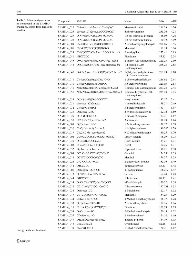
Table 2 Mean unsigned error

by compound in the SAMPL4

challenge, sorted from largest to

smallest

Energy units are kcal/mol

Compound SMILES Name MW AUE

SAMPL4_022 Cc1c(cccc1Nc2ccccc2C(=O)O)C Mefenamic acid 241.29 4.36

SAMPL4_023 c1ccccc1C(c2ccccc2)OCCN(C)C diphenhydramine 255.36 4.28

SAMPL4_027 O(N(=O)=O)C(CCON(=O)=O)C 1,3-bis-(nitrooxy)propane 166.09 4.26

SAMPL4_028 O(N(=O)=O)C(CCON(=O)=O)C 1,3-bis-(nitrooxy)butane 180.12 4.19

SAMPL4_009 Clc1c(C=O)c(Cl)c(OC)c(O)c1OC 2,6-dichlorosyringaldehyde 251.06 3.95

SAMPL4_001 C(C(C(C(C(CO)O)O)O)O)O Mannitol 182.18 3.94

SAMPL4_024 CN(C)CCC=C1c2ccccc2CCc3c1cccc3 Amitriptyline 277.41 3.83

SAMPL4_041 N1CCCCC1 Piperidine 85.15 3.54

SAMPL4_045 O=C1c2c(ccc(N)c2)C(=O)c2c1cccc2 2-amino-9,10-anthraquinone 223.23 2.99

SAMPL4_048 O=C1c2c(C(=O)c3c1cccc3)c(N)ccc2N 1,4-diamino-9,10-

anthraquinone

238.25 2.85

SAMPL4_047 O=C1c2c(cccc2NCCO)C(=O)c2c1cccc2 1-(2-hydroxyethylamino)-

9,10-anthraquinone

267.28 2.68

SAMPL4_011 Clc1c(OC)c(O)c(OC)cc1C=O 2-chlorosyringaldehyde 216.62 2.61

SAMPL4_010 Clc1cc(Cl)c(OC)c(O)c1OC 3,5-dichlorosyringol 223.05 2.54

SAMPL4_046 Nc1c2c(ccc1)C(=O)c3c(cccc3)C2=O 1-amino-9,10-anthraquinone 223.23 2.45

SAMPL4_051 Nc1c2c(c(cc1)O)C(=O)c3c(cccc3)C2=O 1-amino-4-hydroxy-9,10-

anthraquinone

239.23 2.45

SAMPL4_029 O([N?](=O)[O-])CCCCCC Hexyl nitrate 147.17 2.4

SAMPL4_021 c1(ccccc1)Cn2cncc2 1-benzylimidazole 159.214 2.19

SAMPL4_032 Clc1cc(O)ccc1Cl 3,4-dichlorophenol 163 1.97

SAMPL4_035 Oc1ccccc1C=O 2-hydroxybenzaldehyde 122.12 1.89

SAMPL4_025 O(CC(O)C)CCCC 1-butoxy-2-propanol 132.2 1.87

SAMPL4_050 c12c(cc3c(c1)cccc3)cccc2 Anthracene 178.23 1.84

SAMPL4_005 O(C)c1ccccc1OC 1,2-dimethoxybenzene 138.17 1.79

SAMPL4_020 C=C(c1ccccc1)c2ccccc2 1,1-diphenylethene 180.245 1.79

SAMPL4_019 C1c2c(Cc3c1cccc3)cccc2 9,10-dihydroanthracene 180.25 1.76

SAMPL4_002 CC(=CCCC(C)(C=C)OC(=O)C)C Linalyl acetate 196.29 1.73

SAMPL4_030 O(C(=O)C)CCCCCC Hexyl acetate 144.21 1.71

SAMPL4_003 CC(=CCCC(=CCO)C)C Nerol 154.25 1.7

SAMPL4_052 O(c1ccccc1)c1ccccc1 Diphenyl ether 170.21 1.58

SAMPL4_004 OC\ C=C(\ CCC=C(C)C)/ C Geraniol 154.25 1.53

SAMPL4_016 OC1CC(CCC1C(C)C)C Menthol 156.27 1.53

SAMPL4_026 C(C)OCCOC(=O)C 2-Ethoxyethyl acetate 132.16 1.49

SAMPL4_042 O1CCCCC1 Tetrahydropyran 86.13 1.48

SAMPL4_006 Oc1ccc(cc1OC)CCC 4-Propylguaiacol 166.217 1.47

SAMPL4_013 OC1CC(CC=C1C)C(C)=C Carveol 152.24 1.43

SAMPL4_044 O1CCOCC1 1,4-dioxane 88.11 1.41

SAMPL4_014 O=C\ C1=C\CC(\C(=C)C)CC1 l-Perillaldehyde 150.22 1.38

SAMPL4_012 CC1C(=O)CC(CC1)C(=C)C Dihydrocarvone 152.238 1.32

SAMPL4_036 Oc1ccccc1CC 2-Ethylphenol 122.17 1.32

SAMPL4_017 CC1CCC(C(=O)C1)C(C)C Menthone 154.25 1.29

SAMPL4_034 Cc1cc(c(cc1)O)OC 4-Methyl-2-methoxyphenol 138.17 1.28

SAMPL4_033 O(C)c1cccc(OC)c1O 2,6-dimethoxyphenol 154.16 1.26

SAMPL4_015 CC1=CC(=O)C(CC1)C(C)C Piperitone 152.238 1.23

SAMPL4_038 O=Cc1ccccc1C 2-Methylbenzaldehyde 120.15 1.22

SAMPL4_037 COc1c(cccc1)O 2-Methoxyphenol 124.14 1.19

SAMPL4_049 O1c2c(Oc3c1cccc3)cccc2 dibenzo-p-dioxin 184.19 1.15

SAMPL4_043 C1CCC=CC1 Cyclohexene 82.15 1.12

SAMPL4_039 c1cccc(C)c1CC 1-Ethyl-2-methylbenzene 120.2 1.07

146 J Comput Aided Mol Des (2014) 28:135–150

123

submission 197 used the AMSOL solvation model [23]

from the ZINC processing pipeline [24] for hydration free

energy predictions, with conformations predicted by

OpenEye’s Omega [8, 25, 26].

Evaluation of difficult compounds

In order to assess whether some compounds were more

difficult than others, we calculated the average unsigned

error (AUE) across all submissions for each compound in

the set. A low value means that all submissions provided

fairly accurate predictions, while a high value means that

many methods agreed poorly with experiment. Average

errors range from 1.1 to 4.4 kcal/mol as in Table 2, where

compounds are sorted from largest error to smallest.

The ten compounds which were most poorly predicted

(with the largest average error) came from all five groups:

three from group 1, one from group 2, one from group 3, two

from group 4, and three from group 5. So the initial grouping

was not effective at isolating problem compounds.

Instead, we found that the compounds which tended to

be well-predicted were typically fairly simple, without

strongly interacting functional groups, while compounds

which presented more challenges were mostly polyfunc-

tional with several interacting groups. There also seems to

be a tendency for errors to be higher with greater molecular

weight, but molecular weight alone is not a good predictor.

And, since higher molecular weight compounds tend to

have more functional groups, this may simply be due to

increasing complexity.

Still, several compounds stand out as giving particularly

high errors even given their molecular weights. If we fit a

quadratic (passing through zero) to the error versus molec-

ular weight, four compounds in particular stand out as having

higher-than-expected errors. Three of these are unsurpris-

ing—1,3-bis-(nitrooxy)propane, 1,3-bis-(nitrooxy)butane,

and mannitol, all of which are polyfunctional with several

interacting groups. The fourth is surprising: piperidine,

which seems quite simple, yet has an AUE of 3.54 kcal/mol

which is nearly as high as that of mannitol (3.94). Thus, even

simple amines may pose a problem for a variety of methods.

It is also worth noting that piperidine was a ‘‘supplementary’’

compound, meaning the experimental value is relatively

readily available. If we instead do a linear fit to the error

versus molecular weight, several additional compounds have

higher-than-expected errors. These include mefenamic acid,

2,6-dichlorosyringaldehyde, and diphenhydramine. These,

too, are unsurprising given their polyfunctional nature.

The overall tendency we see for error to rise with

molecular weight seems somewhat disconcerting, given that

drug-like molecules can have substantially higher molecular

weights than any of the compounds in this set. Thus further

work may be needed on polyfunctional compounds to

improve accuracies for larger, drug-like molecules.

Of the 47 compounds in the challenge, only 17 had

mean absolute errors less than 1.5 kcal/mol. A further 17

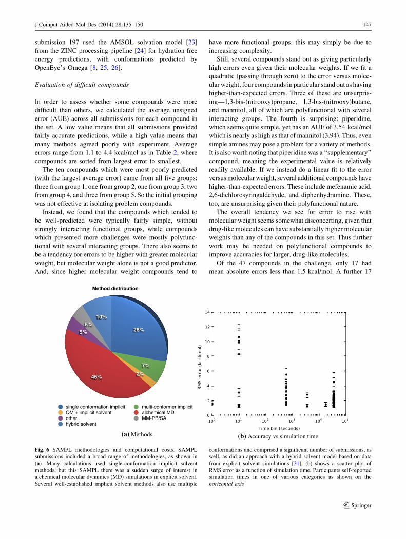
26%

7%

2%45%

5%5%

10%

Method distribution

single conformation implicit multi-conformer implicitQM + implicit solvent alchemical MDother MM-PB/SAhybrid solvent

(a) Methods (b) Accuracy vs simulation time

Fig. 6 SAMPL methodologies and computational costs. SAMPL

submissions included a broad range of methodologies, as shown in

(a). Many calculations used single-conformation implicit solvent

methods, but this SAMPL there was a sudden surge of interest in

alchemical molecular dynamics (MD) simulations in explicit solvent.

Several well-established implicit solvent methods also use multiple

conformations and comprised a significant number of submissions, as

well, as did an approach with a hybrid solvent model based on data

from explicit solvent simulations [31]. (b) shows a scatter plot of

RMS error as a function of simulation time. Participants self-reported

simulation times in one of various categories as shown on the

horizontal axis

J Comput Aided Mol Des (2014) 28:135–150 147

123

had mean absolute errors greater than 2.0 kcal/mol, sug-

gesting further improvement is needed. Thus, we believe

there remains a further need for solvation challenges to

help drive further improvements in solvation modeling.

SAMPL methodologies

SAMPL4 submissions represented a broad range of meth-

odologies (Fig. 6). Interestingly, unlike previous SAMPL

challenges, this challenge saw a surge of interest in explicit

solvent alchemical free energy calculations based on

molecular dynamics simulations, with more submissions in

that category than any other. But single conformation

implicit solvent calculations, such as with Poisson–Boltz-

mann calculations or semi-empirical models such as AM-

SOL, continued to play a major role. As noted above, an

ab initio quantum calculation combined in implicit solvent

also looked interesting in this challenge. Multiple confor-

mation implicit solvent methods (COSMO, FiSH) [27–30]

also continued to play a role, as did a hybrid solvent model

based on data from molecular dynamics simulations. We

also saw several simulations based on an MM-PB/SA

approach. Several newer methods, including a solvent

density functional theory approach, filled out the challenge.

It is difficult to declare any particular class of methods the

‘‘victor’’. As noted above, the top three submissions by most

metrics involved a wide range of methods. As a function of

simulation time, the methods with the lowest computational

cost actually appear best (Fig. 6b), but this is primarily

because there were only two methods in this bracket (149 and

561), both of which did quite well. At the opposite end in

terms of speed are alchemical molecular dynamics simula-

tions, but using these simulations alone was no sure predictor

of success. Simulation details, including force field and

protocol, seem to have mattered a great deal.

As noted above, we also ran two simple knowledge-

based models for comparison purposes, IDs 014 and 015,

which ‘‘predict’’ hydration free energies based assigning

the value of the most similar compound in a database of

knowns (ID 014) or an average of the three most similar

compounds (ID 015). These were in the bottom half of

submissions by every metric of typical error, and per-

formed worst by Kendall tau. We found this encouraging,

as it suggests that even the more empirical methods tested

here are building in substantially more transferability than

a naive approach to knowledge-based modeling. Still, RMS

errors in the vicinity of 3 kcal/mol were possible with this

crude approach.

Significance testing

As noted above, we used Student’s paired t test on the error

of different submissions to examine whether differences

between methods were statistically significant. We find

that, given the relatively small size of the set and the nearly

comparable accuracy of many submissions, that many

differences are in fact not statistically significant. Consider,

for example, the best submission by ranked AUE, sub-

mission 145, with an AUE of 0.87 ± 0.13 kcal/mol.

Comparing this to other submissions via the t test with a

significance threshold of p = 0.01, we find that only sub-

missions 138, 015, 566, 544, 545, 014, 565, 153, 562, 548,

152, 569, 570, and 137 (ordered by significance, from least

to most) yield significantly different predictions. This

represents just 14 submissions out of the 44 full submis-

sions examined here, and attests partially to the fact that the

vast majority of submissions did quite well and yielded

predictions tightly clustered around the true values. If we

adjusted the threshold to p = 0.05, another four submis-

sions would be considered significantly different, but still

more than half of the total submissions are not significantly

different than 145 by this analysis.

We also used the t test to examine how many methods

yielded predictions substantially different from our simi-

larity-based control models, 014 and 015. Here, we found

that some 16 submissions were significantly distinct from

014 (submissions 561, 169, 166, 567, 181, 005, 572, 145,

180, 575, 568, 573, 153, 152, 569, and 570) at p = 0.01,

and 16 from submission 015 (169, 166, 005, 181, 567, 145,

572, 180, 575, 568, 573, 153, 152, 569, and 570). Thus,

while these control models were certainly not top per-

formers, they were also not particularly easy to beat in a

statistically significant way, partly because their typical

errors are not that large. This probably stems from the

substantial size of the database they draw from.

On the whole, we believe these results are encouraging

and indicate that a range of methods are converging on

fairly high accuracy hydration free energy calculations, and

are able to outperform a simple knowledge-based model in

a statistically significant way.

Outlook for method evaluation and error estimation

Overall, we find that relatively little work seems to have

gone into error estimation, but we believe this is extremely

important, since a method which can predict when it will

succeed and fail will be of much more practical value than

one which cannot. Thus error estimation is, we believe, an

important goal for computational methods. In this SAMPL,

most participants estimated a constant error across all

compounds for a given method/submission. So, while some

participants were better than others at giving reasonable

error estimates, error estimates had very little predictive

power. As noted in the analysis section, for example,

submissions which have superficially similar accuracies

148 J Comput Aided Mol Des (2014) 28:135–150

123

may actually have quite different performance when

judged by metrics which reflect their ability to estimate

likely errors.

We believe more work is needed in this area both on our

metrics and from the standpoint of prediction methods. We

still need error metrics which can penalize predictions

which are precise but wrong more than those which are

imprecise and wrong, and reward those which are precise

and correct more than those which are imprecise and cor-

rect. While KL divergence has some of the right properties,

it is unbounded in the case of profound disagreement with

experiment. This is undesirable both from the standpoint of

computing averages, and also because a more realistic

metric would reflect the experimental reality that once a

computational prediction is sufficiently bad, it becomes

effectively useless and, in a discovery setting, would need

to be tested experimentally to be of any value. We are not

yet aware of a metric which has all the necessary properties

in this regard.

At the same time, submitters and methods need to do a

better job estimating error or model uncertainty. To a first

approximation, one could simply compare compounds

being predicted to a library of past predictions, and base

error/uncertainty estimates on performance on similar

compounds in the past. Compounds containing new

chemical functionality not studied previously could be

assigned substantially less confidence. As far as we are

aware, such an experience-based approach has not yet been

applied in SAMPL to help estimate uncertainty.

Conclusions

For the SAMPL4 hydration challenge, a remarkably broad

range of methods were employed, and several very dispa-

rate methods performed remarkably well. Indeed, a sub-

stantial number of submissions typically performed within

error of the top methods, making it difficult to declare clear

winners and losers. One overall sense at the SAMPL4

meeting was that this was actually a plus—many methods

are apparently converging on robust, predictive protocols

with RMS errors under 1.5 kcal/mol. This is encouraging,

and hopefully with further work we can begin to see similar

levels of accuracy in more challenging problems which

comprise the other components of SAMPL—in this case,

host-guest binding and protein-ligand binding.

At the same time, we believe much work still needs to

be done on how best to evaluate methods, and in particular

we would like to see more emphasis from predictors on

providing realistic error estimates. And better metrics to

simultaneously evaluate prediction accuracy and confi-

dence are needed.

Supporting information

In the Supporting Information, we provide full submission

data for all submissions for which participants were willing

to share the data; this includes predicted values, as well as

method descriptions. We also provide the SAMPL chal-

lenge inputs, and error/analysis statistics for the ‘‘blind’’

and ‘‘supplementary’’ components separately. We also give

SMILES strings and IUPAC names for the compounds and

give tables showing results of our t test experiments.

Acknowledgments We acknowledge the financial support of the

National Institutes of Health (1R15GM096257-01A1), and computing

support from the UCI GreenPlanet cluster, supported in part by NSF

Grant CHE-0840513. We also thank J. Peter Guthrie for help with

sorting out structure and naming confusion in SAMPL preparation,

several SAMPL participants including Jens Reinisch and Samuel

Genheden for helpful exchanges on issues with the guaiacol series,

and Andreas Klamt for help on data relating to 1-benzylimidazole.

We also thank OpenEye for their support of the SAMPL meeting and

for running the web server, and Matt Geballe (OpenEye) for help

managing the web site and automated submission system.

References

1. Geballe MT, Guthrie JP (2012) The SAMPL3 blind prediction

challenge: transfer energy overview. J Comput Aided Mol Des

26(5):489–496

2. Geballe MT, Skillman AG, Nicholls A, Guthrie JP, Taylor PJ

(2010) The SAMPL2 blind prediction challenge: introduction and

overview. J Comput Aided Mol Des 24(4):259–279

3. Klimovich P, Mobley DL (2010) Predicting hydration free

energies using all-atom molecular dynamics simulations and

multiple starting conformations. J Comput Aided Mol Des

24(4):307–316

4. Mobley DL, Bayly CI, Cooper MD, Dill KA, Dill KA (2009)

Predictions of hydration free energies from all-atom molecular

dynamics simulations. J Phys Chem B 113:4533–4537

5. Mobley DL, Liu S, Cerutti DS, Swope WC, Rice JE (2012)

Alchemical prediction of hydration free energies for SAMPL.

J Comput Aided Mol Des 26(5):551–562

6. Nicholls A, Mobley DL, Guthrie JP, Chodera JD, Bayly CI,

Cooper MD, Pande VS (2008) Predicting small-molecule solva-

tion free energies: an informal blind test for computational

chemistry. J Med Chem 51(4):769–779

7. Guthrie JP (2014) SAMPL4, a blind challenge for computational

solvation free energies: the compounds considered. J Comput

Aided Mol Des. doi:10.1007/s10822-014-9738-y

8. OpenEye Python Toolkits (2013)

9. Mobley DL, Bayly CI, Cooper MD, Shirts MR, Dill KA (2009)

Small molecule hydration free energies in explicit solvent: an

extensive test of fixed-charge atomistic simulations. J Chem

Theory Comput 5(2):350–358

10. Mobley DL, Dumont E, Chodera JD, Dill K (2007) Comparison

of charge models for fixed-charge force fields: small-molecule

hydration free energies in explicit solvent. J Phys Chem B

111(9):2242–2254

11. Chodera JD, Noe F (2010) Probability distributions of molecular

observables computed from Markov models. II. Uncertainties in

J Comput Aided Mol Des (2014) 28:135–150 149

123

observables and their time-evolution. J Chem Phys

133(10):105,102

12. Press WH, Teukolsky SA, Vetterling WT, Flannery BP (1999)

Numerical recipes in C, 2nd edn. Cambridge University Press,

Cambridge

13. Yang W (2013) Personal Communication

14. Sandberg L (2013) Predicting hydration free energies with

chemical accuracy: The SAMPL4 challenge. J Comput Aided

Mol Des. doi:10.1007/s10822-014-9725-3

15. Ellingson BA, Geballe MT, Wlodek S, Bayly CI, Skillman AG,

Nicholls A (2014) Efficient calculation of SAMPL4 hydration

free energies using OMEGA, SZYBKI, QUACPACK, and Zap

TK. J Comput Aided Mol Des. doi:10.1007/s10822-014-9720-8

16. Nicholls A, Wlodek S, Grant JA (2010) SAMPL2 and continuum

modeling. J Comput Aided Mol Des 24(4):293–306

17. Jakalian A, Jack D, Bayly CI (2002) Fast, efficient generation of

high-quality atomic charges. AM 1(BCC model): II. Parameter-

ization and validation. J Comput Chem 23(16):1623–1641

18. Wang J, Wolf R, Caldwell J, Kollman P, Case D (2011) Devel-

opment and testing of a general amber force field. J Comput

Chem 25(9):1157–1174

19. Fennell CJ, Wymer KL, Mobley DL (2014) Polarized alcohol in

condensed-phase and its role in small molecule hydration

20. Muddana HS, Sapra NV, Fenley AT, Gilson MK (2014) The

SAMPL4 hydration challenge: evaluation of partial charge sets

with explicit-water molecular dynamics simulations. J Comput

Aided Mol Des. doi:10.1007/s10822-014-9714-6

21. Canzar S, El-Kebir M, Pool R, Elbassioni K, Malde AK, Mark AE,

Geerke DP, Stougie L, Klau GW (2013) Charge group partitioning

in biomolecular simulation. J Comput Biol 20(3):188–198

22. Malde AK, Zuo L, Breeze M, Stroet M, Poger D, Nair PC,

Oostenbrink C, Mark AE (2011) An automated force field

topology builder (ATB) and repository: version 1.0. J Chem

Theory Comput 7(12):4026–4037

23. Hawkins GD, Giesen DJ, Lynch GC, Chambers CC, Rossi I,

Storer JW, Li J, Zhu T, Thompson J, Winget P, Lynch BJ AM-

SOL. http://comp.chem.umn.edu/amsol/

24. Irwin JJ, Sterling T, Mysinger MM, Bolstad ES, Coleman RG

(2012) ZINC: a free tool to discover chemistry for biology.

J Chem Inf Model 52(7):1757–1768

25. Hawkins PCD, Nicholls A (2012) Conformer generation with

OMEGA: learning from the data set and the analysis of failures.

J Chem Inf Model 52(11):2919–2936

26. Hawkins PCD, Skillman AG, Warren GL, Ellingson BA, Stahl

MT (2010) Conformer generation with OMEGA: algorithm and

validation using high quality structures from the Protein Data-

bank and Cambridge structural database. J Chem Inf Model

50(4):572–584

27. Hogues H, Sulea T, Purisima EO (2014) Exhaustive docking and

solvated interaction energy scoring: lessons learned from the

SAMPL4 challenge. J Comput Aided Mol Des. doi:10.1007/

s10822-014-9715-5

28. Klamt A, Eckert F, Diedenhofen M (2009) Prediction of the free

energy of hydration of a challenging set of pesticide-like com-

pounds. J Phys Chem B 113(14):4508–4510

29. Reinisch J, Klamt A (2014) Prediction of free energies of

hydration with COSMO-RS on the SAMPL4 data set. J Comput

Aided Mol Des. doi:10.1007/s10822-013-9701-3

30. Sulea T, Purisima EO (2011) Predicting hydration free energies of

polychlorinated aromatic compounds from the SAMPL-3 data set

with FiSH and LIE models. J Comput Aided Mol Des 26(5):661–667

31. Li L, Dill KA, Fennell CJ (2014) Hydration assembly tests in the

SAMPL4 challenge. J Comput Aided Mol Des. doi:10.1007/

s10822- 014-9712-8

150 J Comput Aided Mol Des (2014) 28:135–150

123