Optics Communications 285 (2012) 5051–5061

Contents lists available at SciVerse ScienceDirect

Optics Communications

0030-40

http://d

n Corr

E-m

journal homepage: www.elsevier.com/locate/optcom

Blind image deconvolution using the Fields of Experts prior

Wende Dong, Huajun Feng n, Zhihai Xu, Qi Li

State Key Laboratory of Modern Optical Instrumentation, No.38, Zheda road, West Lake district, Hangzhou city, Zhejiang province 310027, China

a r t i c l e i n f o

Article history:

Received 7 January 2012

Received in revised form

30 July 2012

Accepted 16 August 2012Available online 31 August 2012

Keywords:

Blind image deconvolution

Fields of Experts (FoE) prior

Student-t prior

Alternating minimization (AM) approach

18/$ - see front matter & 2012 Elsevier B.V. A

x.doi.org/10.1016/j.optcom.2012.08.041

esponding author. Tel./fax: þ86 571 8795118

ail address: fenghj@zju.edu.cn (H. Feng).

a b s t r a c t

In this paper, we present a method for single image blind deconvolution. To improve its ill-posedness,

we formulate the problem under Bayesian probabilistic framework and use a prior named Fields of

Experts (FoE) which is learnt from natural images to regularize the latent image. Furthermore, due to

the sparse distribution of the point spread function (PSF), we adopt a Student-t prior to regularize it. An

improved alternating minimization (AM) approach is proposed to solve the resulted optimization

problem. Experiments on both synthetic and real world blurred images show that the proposed method

can achieve results of high quality.

& 2012 Elsevier B.V. All rights reserved.

1. Introduction

In photography, image blurring is often caused by defocusing,atmospheric disturbance, relative motion, etc. Noise may also beintroduced owing to the quantization error, recording deviceand so on. The degradation process is modeled by convolvingthe latent image with a point spread function (PSF) plus somenoise, i.e.,

g¼ kfþn ð1Þ

where g, f and n represent the vector forms of the blurred image,latent image and noise respectively, k is the convolution matrix ofthe PSF. In frequency domain, it is formulated by

GðuÞ ¼ KðuÞFðuÞþNðuÞ ð2Þ

where G(u), K(u), F(u) and N(u) denote the discrete FourierTransforms of the blurred image, PSF, latent image and noiserespectively.

The inverse process of image blurring is called image decon-volution which aims to restore the latent image from the blurred.There are two kinds of image deconvolution methods in termsof whether the PSF is known, i.e., blind and non-blind imagedeconvolution.

In blind image deconvolution, we need to restore both thelatent image and PSF from the blurred. There are many appro-aches of this kind, e.g., in [1], the authors propose a methodbased on the Richardson–Lucy (RL) algorithm (RL algorithm is anon-blind image deconvolution method [2,3]). In [4], the authors

ll rights reserved.

2.

present an asymmetric multiplicative iterative algorithm. How-ever, since the problem is severely ill-posed, the restored imagesare often contaminated by amplified noise and ringing. Toimprove its ill-posedness, researchers have designed variousregularization methods, such as the Tikhonov regularization [5]and total variation (TV) regularization [6,7].

Blind image deconvolution can also be formulated underBayesian probabilistic framework where the priors of the latentimage and PSF play the role of regularization. In recent years, dueto the usage of some well designed priors, effective blind imagedeconvolution methods emerge. For example, the authors of [8]used two mixture of Gaussian functions to model the sparsedistributions of the natural image gradients and PSF respectively,then a variational Bayesian approach is adopted to compute thePSF, the blurred image is finally restored with the RL algorithm. In[9], the authors also adopt the natural image gradient prior forregularization but use a piecewise function to model it. The PSF isregularized with an l1-norm based prior. The resulted maximum aposteriori (MAP) estimation problem is solved with a variablesplitting approach. In [10], the latent image is regularized with anew prior based on the responses of some edge detectors and thePSF is regularized with the TV, the latent image and PSF arealternately estimated until convergence. In [11], the noise termn is assumed to follow Poisson distribution and a prior based onthe Huber–Markov random field is introduced. The latent imageand PSF are estimated using the expectation maximization (EM)algorithm. In [12], the authors use a normalized sparse prior toregularize the high frequency components of the latent image.The PSF is estimated with an alternating minimization (AM)approach and the blurred image is restored with the non-blinddeconvolution method proposed in [13]. In [14], the weights of the

W. Dong et al. / Optics Communications 285 (2012) 5051–50615052

PSF (the authors model the PSF as a linear weighted combination ofGaussian kernel functions), local image differences and the imagingmodel errors are all modeled with Student-t priors, the resultedproblem is solved with a variational Bayesian inference method.However, since these approaches are complicated, the optimizationprocess is slow. To solve this problem, the authors of [15] design afast blind deconvolution method, it uses the shock filter to predictthe sharp edges of the latent image and adopt Gaussian priors forregularization. Since the shock filter is simple and the resultedquadratic optimization problem can be solved efficiently, thisalgorithm is very fast. Furthermore, the GPU technique is alsoutilized to accelerate the optimization. Blind image deconvolutionalso includes the approaches using more than one images, e.g., themethods adopting image pairs [16–19] or multi-frames [20–24].

There are also many approaches for non-blind image decon-volution in which the PSF is obtained in advance (e.g., in remotesensing, the PSF is usually calculated using the edge method [25]),such as the famous Wiener filtering [26] and Richardson–Lucy(RL) algorithm [2,3]. However, even the PSF is known, non-blindimage deconvolution is also ill-posed, so regularization is neces-sary, e.g., the methods using Tikhonov regularization [27], TVregularization [28–30], sparse prior regularization [31], GaussianMarkov random field regularization [32] and so on.

From the above, we can see that priors play an important rolein image deconvolution, but constructing image priors is achallenging task due to their high dimensionality, non-Gaussianstatistics, and the need to model relations over extended neigh-borhoods. In previous work such as [8,9,31], the latent image ismodeled by formulating the responses of difference filters withGaussian or sparse distributions. However, since both the filtersand parameters are handcrafted, they are lack of variations and

Fig. 1. (a) The learnt filters which are used to construct the FoE prior. (b) A natural imag

natural image shown in (b) with the first filter shown in (a)) and the Student-t functio

may not capture the features of the latent image accurately. Toimprove the situation, in [33], the authors propose a robust priornamed Fields of Experts (FoE) for natural images, all its filters andparameters of the potential function are learnt from naturalimages, experiments on image denoising and inpainting haveexhibited its effectiveness. In this paper, we introduce this priorinto blind image deconvolution to regularize the latent image.Furthermore, unlike the previous work in which the PSF ismodeled with TV [6] or l1-norm based prior [9], we adopt aStudent-t prior to regularize it. Although it is simpler than theStudent-t prior used in [14], it fits the distribution of the PSF wellenough to ensure a good result. To solve the resulted Bayesianmodel, we propose an improved AM algorithm to estimate thePSF and use a non-blind image deconvolution method which alsoadopts the FoE prior to restore the blurred image. Experiments onboth synthetic and real world blurred images show that theresults are comparable with that of some state of the art methods.

The rest of the paper is organized as follow. In section 2, wemake a description of the adopted priors and formulate theproblem under Bayesian framework. In section 3, we demonstratethe optimization approach. In section 4, the proposed method istested using both synthetic and real world blurred images. Finally,a conclusion is made in section 5.

2. Problem formulation

Under Bayesian framework, blind image deconvolution is formu-lated by the following MAP estimation problem:

ðf,kÞ ¼ arg maxðf,kÞPðf,k9gÞ ¼ arg maxðf,kÞPðg9f,kÞ*PðfÞ*PðkÞ ð3Þ

e. (c) The empirical probabilistic distribution of the filter response (convolving the

n used model it.

Fig. 2. (a) PSF1: a Gaussian PSF. (b) PSF2: a motion caused PSF. (c) The probabilistic distributions of the PSFs and the Student-t prior used to model them.

W. Dong et al. / Optics Communications 285 (2012) 5051–5061 5053

Take the negative logarithm of Eq. (3), it is converted into thefollowing equation, i.e.,

ðf,kÞ ¼ arg minðf,kÞ½�ln Pðg9f,kÞ�ln PðfÞ�ln PðkÞ� ð4Þ

There are three terms �lnPðg9f,kÞ, �lnPðfÞ and �lnPðkÞ thatneed to be modeled in Eq. (4). Suppose that the conditionallikelihood P(g9f,k)follows a Gaussian distribution, then

�lnPðg9f,kÞp:kf�g:2

2 ð5Þ

To model the term P(f), we adopt the FoE prior proposed in [33]which is essentially a Markov random field. With Hammersley–Clifford theorem [34], the FoE model for P(f) can be expressed by

PðfÞ ¼1

Z

Yi

YJ

j ¼ 1

fjðwTj fðiÞ; ajÞ ð6Þ

fjðwTj fðiÞ; ajÞ ¼ 1þ

1

2ðwT

j fðiÞÞ2

� ��aj

ð7Þ

where i and j denote the pixel index and filter index respectively,J is the total number of filters used to construct the prior, eachwj denotes a learnt filter, f(i) represents a clique centered on thei-th pixel and wT

j fðiÞ is the result of convolving f(i) with the filterwj, Z is a normalizing constant. In contrast to the previous priors,all the filters and parameters of the FoE prior are learnt fromnatural images using a method called contrastive divergence.

The principle of the FoE prior is, if we convolve a natural imagewith an arbitrary learnt filter wj, the response follows a heavy-tailed distribution which can be properly fitted by the Student-tfunction shown in Eq. (7). Taking the products of the responses ofseveral filters makes it more robust to model natural images.

We take an example in Fig. 1 to demonstrate the features ofthe FoE prior. Fig. 1(a) shows the learnt filters which are used toconstruct the prior. Fig. 1(b) is a natural image, convolving it withthe first filter in Fig. 1(a), the blue curve in Fig. 1(c) shows theempirical distribution of the response and the red curve repre-sents the Student-t function used to model it. In [33], the authorshave pointed out that the typical handcrafted priors just considersimple nearest neighbor relations that they can only crudelycapture the statistics of natural images. While in the FoE prior,all the filters are larger and of more complex structures, whichmeans the relations between the pixels in a larger local area in theimage are considered. Furthermore, unlike the handcrafted priors,all the filters and other parameters of the FoE prior are learnt fromnatural images using the mathematical approach, thus it can

model the probabilistic distribution of the natural images moreaccurately.

From Eq. (6) and (7), we obtain that

�lnPðfÞ ¼ lnðZÞþX

i

XJ

j ¼ 1

ajln 1þ1

2ðwT

j fðiÞÞ2

� �ð8Þ

The next task is to model the term P(k). In most cases, the PSFk follows a sparse distribution, e.g., in a motion caused PSF, mostof the elements are zeros. In [8], the authors use a mixture ofGaussian functions to model it, while in [9] it is modeled by anl1-norm based prior. In this paper, we adopt a Student-t functionto model it, i.e.,

PðkÞpY

l

½1þmðklÞ2��g ð9Þ

where l denotes the element index in k, m and g are twocoefficients for the Student-t function, so

�lnPðkÞpX

l

ln½1þmðklÞ2� ð10Þ

Fig. 2(a) and (b) show two PSFs, one is a Gaussian PSF and theother is a motion caused PSF. In Fig. 2(c), the red and green curvesrepresent the empirical distributions of the two PSFs respectively,the blue curve denotes the proposed Student-t prior (Eq. (9)) usedto model them. We can see that although it is simpler than theStudent-t prior used in [14], it fits the distributions of the PSFswell, which is enough to ensure a good result.

From Eqs. (4), (5), (8) and (10), we obtain that

ðf,kÞ ¼ arg minðf,kÞl2:kf�g:2

2þX

i

XJ

j ¼ 1

ajln 1þ1

2ðwT

j fðiÞÞ2

� �8<:

þx2

Xl

ln½1þmðklÞ2�

)ð11Þ

where l and x are the regularization coefficients.

3. The optimization approach

Just like the method in [8], our blind image deconvolutionapproach consists of two phases, i.e., we first estimate the PSFfrom Eq. (11) with an improved AM algorithm and then use theestimated PSF to deblur the image. The details are given in thefollowing subsections.

W. Dong et al. / Optics Communications 285 (2012) 5051–50615054

3.1. The general alternating minimization (AM) approach for PSF

estimation

The most commonly used method to solve the problem inEq. (11) is the AM approach (e.g., in [5,10]) which is realizedby iteratively implementing the following two steps untilconvergence:

(i) Fix the PSF obtained from a certain iteration and estimatethe latent image for the next iteration, i.e.,

ftþ1¼ arg minf

l2:ktf�g:2

2þX

i

XJ

j ¼ 1

ajln 1þ1

2ðwT

j fðiÞÞ2

� �8<:

9=; ð12Þ

(ii) Fix the latent image and estimate the PSF, i.e.,

ktþ1¼ arg mink

l2:kftþ1

�g:2

2þx2

Xl

ln½1þmðklÞ2�

( )ð13Þ

where t is the iteration number.Eq. (12) is essentially a non-blind image deconvolution

problem. To solve it efficiently, we adopt the variable splittingapproach proposed in [13,28]. We first introduce J auxiliaryvariables vj (j¼1, 2, y, J) and convert Eq. (12) into the followingequation (to make a clear description, we have removed thesuperscript t and tþ1)

f ¼ arg minfl2:kf�g:2

2þb2

Xi

XJ

j ¼ 1

aj ðvjÞi�wTj fðiÞ

h i2

8<:

þX

i

XJ

j ¼ 1

ajln 1þ1

2ðvjÞ

2i

� �9=; ð14Þ

where (vj)i denotes the i-th element in vj. As b-N, the solutionof Eq. (14) converges to that of Eq. (12).

In practice, b is usually initialized with 1 and increased bymultiplying a scale factor R (R41). For each given b, we first fix f(if b¼1, f is initialized with the blurred image g) and estimate allthe terms (vj)i, i.e.,

ðvjÞi ¼ arg minðvjÞiJ ðvjÞi� �

¼ arg minðvjÞi

b2ðvjÞi�wT

j fðiÞh i2

þ ln 1þ1

2ðvjÞ

2i

� �� �ð15Þ

Since Eq. (15) is differentiable, its solution can be chosen fromthe real roots of J

0

[(vj)i]¼0(it is essentially a cubic equationand the three roots can be calculated with certain formula).However, we find that the root finding and choosing process istime-consuming, so we turn to use the Newton–Raphson method,

Fig. 3. (a) Flow chart of step (i) for the general AM algorithm. (b) Flow chart of the whole

T is the total number of iterations).

i.e.,

ðvjÞnþ1i ¼ ðvjÞ

ni �

J0½ðvjÞni �

J00½ðvjÞni �

ð16Þ

where J0

and J00denote the first and second derivatives of J, n is theiteration number for the Newton–Raphson method.

After all the variables vj (j¼1, 2,y, J) are calculated, the nexttask is to estimate f, i.e.,

f ¼ arg minfl2:kf�g:2

2þb2

Xi

XJ

j ¼ 1

aj ðvjÞi�wTj fðiÞ

h i2

8<:

9=; ð17Þ

It is equal to Eq. (18) and can be solved efficiently in frequencydomain by Eq. (19)

f ¼ arg minfl2:kf�g:2

2þb2

XJ

j ¼ 1

aj:vj�wTj f:2

2

8<:

9=; ð18Þ

FðuÞ ¼lKnðuÞGðuÞþb

PJj ¼ 1 ajW

n

j ðuÞVjðuÞ

lKnðuÞKðuÞþb

PJj ¼ 1 ajW

n

j ðuÞWjðuÞð19Þ

where Wj(u) and Vj(u) represent the discrete Fourier transforms ofthe variables wj and vj, the superscript n denotes the complexconjugation, f can be calculated using the inverse discrete Fouriertransform.

After f is obtained, we increase b by b¼b*R and start anotherround of optimization for the auxiliary variables. The alternatingprocess is terminated until b reaches bmax. The flow chart for step(i) is shown in Fig. 3(a). Here, we should point out that since theFoE prior is very robust in modeling the latent image, the abovedescribed algorithm is an effective non-blind deconvolutionmethod. In subsection 3.3, it will be used to improve the qualityof the restored image.

To solve the problem in Eq. (13), we adopt the iterativelyreweighted least squares (IRLS) method. Assuming that jðklÞ ¼

ln½1þmðklÞ2� (to make a clear description, we have removed the

superscript tþ1), then the reweighted term for kl (where kl

denotes the l-th element in k) is

fðklÞ ¼1

kl

djðklÞ

dkl¼

2m

1þmðklÞ2

ð20Þ

and the reweighted matrix is K¼diag[j(kl)], i.e., K is a diagonalmatrix whose l-th element on the diagonal is j(kl).

In IRLS, the matrix K in each iteration is constructed with the kobtained from the former iteration, i.e., Kpþ1

¼ diag½fðkpl Þ� (where

general AM algorithm (where t denotes the iteration number in Eqs. (12) and (13),

Fig. 4. (a) Flow chart of step (i) for the improved AM algorithm (where t denotes the iteration number in Eqs. (12) and (13)). (b) Flow chart of the whole improved

AM algorithm.

W. Dong et al. / Optics Communications 285 (2012) 5051–5061 5055

p is the iteration number for IRLS). So

kpþ1¼ arg mink

l2:kf�g:2

2þx2

kT Kpþ1k

� �ð21Þ

which can be solved with the conjugate gradient (CG) method.But in this paper, we make some changes on it and result in thefollowing equation:

kpþ1¼ arg mink

l2:kT1ðdfÞ�dg:2

2þx2

kT Kpþ1k

� �ð22Þ

where d¼d1þd2, d1 and d2 are the vertical and horizontaldifference filters, i.e., [�1, 1] and [�1, 1]T. T1(f)is a pixel-wisethreshold function defined by

T1ðf iÞ ¼0 if f ircf

f i else

(ð23Þ

where cf is a constant, fi denotes the i-th pixel in f.There are two advantages of Eq. (22) over Eq. (21). Firstly, the

authors of [15] have shown that using difference filters on f and gcan accelerate the convergence of the CG method. Secondly, thethreshold function T1(f) eliminates the inaccurate tiny textures indf caused by noise and ringing, which helps to improve theaccuracy of the estimated PSF.

After the PSF is estimated, we also adopt a pixel-wise thresh-old function T2(kl) to remove the noise, i.e.,

T2ðklÞ ¼0 if klr maxðkÞnck

kl else

(ð24Þ

where ck is a constant. Then the estimated PSF is normalized bykl ¼ kl=

Plkl. The flow chart of the whole general AM algorithm is

shown in Fig. 3(b).

3.2. An improved alternating minimization (AM) approach for PSF

estimation

But in practice, we find that the general AM approach usuallydoes not converge to a satisfactory result, e.g., in the experimentshown in Fig. 6, both its estimated PSF and restored image are ofrelatively low quality. This phenomenon may be explained by thetheory presented in [35]. The authors of [35] analyze the limita-tions of the MAP estimation method for single image blinddeconvolution and indicate that the general AM algorithm tendsto converge to a blurry solution. To achieve a better result, wepropose an improved version of the above AM approach. The new

flow charts of step (i) and the whole algorithm are shown inFig. 4(a) and (b) respectively.

Comparing Fig. 4(b) with Fig. 3(b), we can see that there is anew coefficient Z, just like the b in Fig. 3(a), it is initialized with1 and increased with the same scale factor R. The differencebetween Figs. 4(a) and 3(a) is the initialization. From Fig. 3(a) weknow that the step (i) of the general AM algorithm always startsfrom the blurred image, so the latent image estimated from thelast iteration is abandoned, while in the improved AM algorithm(Fig. 4(a)), it is used for initialization in the new iteration.Furthermore, since b is initialized with Z in step (i) and Z isincreased with the same rate as b, after certain iterations, theinitialized b will be large enough in Eq. (14) to keep the quality ofmid-restored image and PSF at a high level. With these changes,the performance of the AM algorithm will be much improved, e.g.,in Fig. 6, we can see that the improved AM algorithm converges toa better result than the general AM algorithm. In addition,because b is initialized with Z in the improved AM algorithm,the inner iterations of step (i) will be less than that of the generalAM algorithm when Z41, thus it is faster than the general AMalgorithm.

3.3. Image restoration

Although we can obtain a restored image from the improvedAM approach, its quality is not high enough. This is because in theoptimization process, we must assign l a relatively small value toensure the latent image estimated from step (i) free of noise andringing, otherwise, the negative artifacts will in turn affect theaccuracy of the estimated PSF. To achieve a restored image ofhigher quality, we only use the PSF estimated by the improvedAM algorithm, then we assign l a larger value and adopt the non-blind image deconvolution method which is used to solve theproblem in step (i) of the general AM approach (the flow chart isshown in Fig. 3(a)) to deblur the image. Due to the robustnessof the FoE prior, it can evidently improve the quality of therestored image.

3.4. Implementation details

To use the proposed method, we should first initialize the PSFwith a Gaussian PSF whose size is larger than the ground truth.l is chosen between 300 and 1500 in the phase of PSF estimation,while for image restoration, it is chosen between 500 and 2000.The values of the parameters x and m are empirically set to

Fig. 5. (a) The clear image. (b) Blurred image and the PSF, the noise is zero-mean Gaussian with standard deviation s¼0.01. (c) The PSF estimated with the method

in [8] and the image restored with the method in [13]. (d) The result of the method in [9]. (e) The result of the proposed method.

Table 1SNR and SSIM values of corresponding figures in Fig. 5.

Fig. 5(b) Fig. 5(c) Fig. 5(d) Fig. 5(e)

SNR (dB) 14.18 21.44 21.52 22.31

SSIM 0.64 0.90 0.89 0.91

W. Dong et al. / Optics Communications 285 (2012) 5051–50615056

0.2 and 5 respectively. The scale factor R is set between 2 and 3,and the value for bmax is larger than 216. The parameter cf ischosen between 10 and 20 while ck is chosen between 0.05 and0.15. For the Newton–Raphson method, the stopping criterion isthe absolute value of the error between two consecutive itera-tions is smaller than 1/10,000, i.e., ðvjÞ

nþ1i �ðvjÞ

ni

��� ���o1=10,000,where n is the iteration number for the Newton–Raphson method,i is the element index in vj. For the IRLS algorithm, the stoppingcriterion is, for each element in k, the absolute value of the errorbetween two consecutive iterations is smaller than 1/10,000, i.e.,

kpþ1l �kp

l

��� ���o1=10,000, where p is the iteration number for IRLS, l

is the element index in k.Furthermore, if the size of the PSF is large, we adopt the multi-

scale optimization approach [8,15], i.e., we first down-sample theblurred image to form an image pyramid and estimate the PSF inthe coarsest scale, then the estimated PSF is up-sampled as aguide for the PSF estimation in the adjacent finer scale, theprocess is repeated until it reaches the finest scale and the finallyestimated PSF is obtained. The down-sampling factor betweenadjacent scales is

ffiffiffi2p

.

4. Experimental results

In this section, we use both synthetic and real world blurredimages to demonstrate the effectiveness of the proposed method.We compare it with two state of the art methods which areproposed in [8] and [9]. However, since in [8], the RL algorithm isused to restore the blurred image, the result is contaminated bynoise and ringing, we substitute the RL algorithm with a morerobust non-blind deconvolution method proposed in [13]. Wealso take an example to compare the performances of the generaland improved AM algorithms. Furthermore, the performances ofthe FoE prior regularization and another two more popularregularization methods i.e., the Tikhonov-like regularization andthe TV regularization are also compared.

We adopt SNR and another effective method named StructuralSimilarity and Index (SSIM) [36] to evaluate the restored images.SSIM is designed based on human visual perception and con-sidering three components, i.e., local luminance, local contrastand structure to assess an image. Eq. (25) is its expression

SSIM¼ LaCbSg ð25Þ

where L, C and S denote the comparison functions for localluminance, local contrast and structure respectively, a, b, g40.

4.1. Experiments using synthetic blurred images

Fig. 5(a) is a clear image, it is convolved with a PSF which isshown in the top-left inset in Fig. 5(b) and noised with zero-meanGaussian noise whose standard deviation is 0.01. The degradedimage is shown in Fig. 5(b). Fig. 5(c) and (d) show the estimatedPSFs and restored images of the methods proposed in [8] and [9]respectively (for the method in [8], we only use the estimatedPSF, the blurred image is restored with the method in [13]).Fig. 5(e) shows the PSF estimated by the improved AM algorithmand the image restored with the method proposed in subsection3.3. The SNR and SSIM values of corresponding figures are givenin Table 1. We can see that the PSF estimated by the improved AMalgorithm is the most similar to the true PSF and our non-blinddeconvolution method achieves the best result.

We also make a comparison about the performances of thegeneral and improved AM approaches, the parameters of bothmethods are tuned to ensure the best results. The directly restoredimages (without the assistance of the non-blind deconvolution

Fig. 6. Directly obtained results of the general and improved AM algorithms. (a) The directly restored image of the general AM algorithm (SNR¼20.89 dB, SSIM¼0.89).

(b) The directly restored image of the improved AM algorithm (SNR¼21.65 dB, SSIM¼0.89). (c) The true and the estimated PSFs: the top is the true PSF, the bottom-left

and bottom-right are the PSFs estimated by the general and improved AM algorithms respectively.

Fig. 7. (a) The clear image. (b) Blurred image and the PSF, the noise is zero-mean Gaussian with standard deviation s¼0.01. (c) The result of the method in [9].

(d) The result of the proposed method.

Table 2SNR and SSIM values of corresponding figures in Fig. 7.

Fig. 7(b) Fig. 7(c) Fig. 7(d)

SNR (dB) 20.08 24.28 24.40

SSIM 0.68 0.84 0.84

W. Dong et al. / Optics Communications 285 (2012) 5051–5061 5057

method proposed in subsection 3.3) of the two algorithms arepresented in Fig. 6(a) and (b) respectively, Fig. 6(c) exhibits the truePSF and the estimated PSFs. Both visual perception and assessmentvalues show that the result of the improved AM approach is better.

Fig. 7 is another example in which the ‘‘Lena’’ image (Fig. 7(a))is blurred by a larger and more complex PSF, the additive noise iszero-mean Gaussian with standard deviation s¼0.01, the truePSF and degraded image are shown in Fig. 7(b). Just like in Fig. 5,we compare the result of our method with that of the methodsproposed in [8] and [9]. However, maybe due to the contents ofthe blurred image, the method in [8] fails to estimate the PSF.Fig. 7(c) shows the result of the method proposed in [9] andFig. 7(d) presents the result of our approach. We can see that the

PSF obtained by the improved AM algorithm is more accurate, theSNR and SSIM values in Table 2 also show that the restored imageof the proposed method is better.

From section 2, we see that the FoE prior is robust in modelingthe probabilistic distribution of natural images, and it has been

Fig. 8. The results using Tikhonov-like regularization. (a) The result of the blurred image shown in Fig. 5(b). (b) The result of the blurred image shown in Fig. 7(b).

Fig. 9. The results using TV regularization. (a) The result of the blurred image shown in Fig. 5(b). (b) The result of the blurred image shown in Fig. 7(b).

Table 3SNR and SSIM values of corresponding figures in Figs. 8 and 9.

Fig. 8(a) Fig. 8(b) Fig. 9(a) Fig. 9(b)

SNR (dB) 19.64 21.14 21.79 24.30

SSIM 0.83 0.76 0.89 0.84

W. Dong et al. / Optics Communications 285 (2012) 5051–50615058

successfully used as a regularization term for image denoisingand inpainting [33]. To prove its effectiveness in the applicationof blind image deconvolution, in the following paragraphs,we will make a comparison between the FoE prior regularizationand another two more popular regularization methods, i.e., theTikhonov-like regularization (the Tikhonov-like regularization isdefined as Q ðfÞ ¼

PJj ¼ 1 :djf:

2

2, where dj (j¼1, 2, y, J) denote theconvolution matrices of certain difference filters. If all dj (j¼1, 2,y, J) are identity matrices, Q(f) is the standard Tikhonov regular-ization) and the TV regularization.

In the experiment shown in Fig. 8, we replace the regulariza-tion term for the latent image in Eq. (11) with the Tikhonov-likeregularization and obtain a new equation

ðf,kÞ ¼ arg minðf,kÞl2:kf�g:2

2þX2

j ¼ 1

:djf:2

2þx2

Xl

ln½1þmðklÞ2�

8<:

9=;ð26Þ

where dj (j¼1, 2) represent the convolution matrices of thevertical and horizontal difference filters.

While in the experiment presented in Fig. 9, the TV regular-ization term is used to regularize the latent image and Eq. (11) isrewritten as

ðf,kÞ ¼ arg minðf,kÞl2:kf�g:2

2þX

i

ffiffiffiffiffiffiffiffiffiffiffiffiffiffiffiffiffiffiffiffiffiffiffiffiffiffiffiffiffiffiffiðd1fÞ2i þðd2fÞ2i

qþx2

Xl

ln½1þmðklÞ2�

( )

ð27Þ

To make a fair comparison with the FoE prior regularization,we also use the improved AM algorithm to solve the problems inEqs. (26) and (27). Just like in subsection 3.3, we only use theestimated PSFs. Then the blurred images are restored with thecorresponding regularization methods. The details of the optimi-zation process are given in the appendix, and the SNR and SSIMvalues are presented in Table 3.

From the results, we can see that the Tikhonov-like regular-ization does not perform well. This is because it essentially tendsto overly smooth the sharp image edges which will affect theestimation of the PSF. In contrast, the TV regularization performsbetter and the FoE prior regularization achieves the best result.

4.2. Experiments using real world blurred images

Since there are many differences between the synthetic andreal world blurred images, besides the above experiments, we

Fig. 10. (a) Blurred image of a toy rabbit. (b) The PSF estimated with the method in [8] and the image restored with the method in [13]. (c) The result of the method in [9].

(d) The result of the proposed method. (e–h) Zoom of the contents in the green rectangle of corresponding figures.

Fig. 11. (a) Blurred image of a microscope. (b) The PSF estimated with the method in [8] and the image restored with the method in [13]. (c) The result of the method

in [9]. (d) The result of the proposed method. (e–h) Zoom of the contents in the green rectangle of corresponding figures.

W. Dong et al. / Optics Communications 285 (2012) 5051–5061 5059

also use two color blurred images which are captured by a digitalcamera to test our approach. The results are shown in thefollowing experiments.

In Fig. 10(a) and 11(a), two real world blurred photographs arepresented. We first adopt the methods in [8] and [9] to deal withthem (for the method in [8], we only use the estimated PSF, theblurred image is restored with the method in [13]), the estimatedPSFs and restored images are shown in Figs. 10(b and c) and11(b and c) respectively.

To use the proposed method, we first convert the color imagesinto grayscale ones and estimate their PSFs with the improved AMalgorithm. Then we use the non-blind deconvolution methodproposed in subsection 3.3 to restore the RGB channels of theblurred images separately. The results are shown in Figs. 10(d)and 11(d). Figs. 10(e and h) and Fig. 11(e and h) are the zoom ofthe contents in the green rectangles of corresponding figures, wecan see that the results of our approach are comparable with thatof the other two methods.

W. Dong et al. / Optics Communications 285 (2012) 5051–50615060

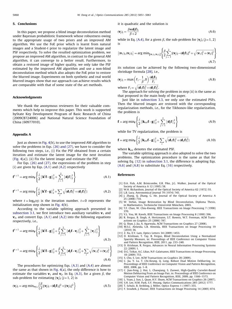
5. Conclusions

In this paper, we propose a blind image deconvolution methodunder Bayesian probabilistic framework whose robustness owingto the appropriate usage of two priors and an improved AMalgorithm. We use the FoE prior which is learnt from naturalimages and a Student-t prior to regularize the latent image andPSF respectively. To solve the resulted optimization problem, wepropose an improved AM algorithm, in contrast to the general AMalgorithm, it can converge to a better result. Furthermore, toobtain a restored image of higher quality, we only take the PSFestimated by the improved AM algorithm and use a non-blinddeconvolution method which also adopts the FoE prior to restorethe blurred image. Experiments on both synthetic and real worldblurred images show that our approach can achieve results whichare comparable with that of some state of the art methods.

Acknowledgments

We thank the anonymous reviewers for their valuable com-ments which help to improve this paper. This work is supportedbyState Key Development Program of Basic Research of China(2009CB724006) and National Natural Science Foundation ofChina (60977010).

Appendix A

Just as shown in Fig. 4(b), to use the improved AM algorithm tosolve the problems in Eqs. (26) and (27), we have to consider thefollowing two steps, i.e., (i) Fix the PSF obtained from a certainiteration and estimate the latent image for the next iteration(Fig. 4(a)). (ii) Fix the latent image and estimate the PSF.

For Eqs. (26) and (27), the expressions of the problem in step(i) are given by Eqs. (A.1) and (A.2) respectively

ftþ1¼ arg minf

l2:ktf�g:2

2þX2

j ¼ 1

:djf:2

2

8<:

9=; ðA:1Þ

ftþ1¼ arg minf

l2:ktf�g:2

2þX

i

ffiffiffiffiffiffiffiffiffiffiffiffiffiffiffiffiffiffiffiffiffiffiffiffiffiffiffiffiffiffiffiðd1fÞ2i þðd2fÞ2i

qg

(ðA:2Þ

where t¼ logRðZÞ is the iteration number. t¼0 represents theinitialization step shown in Fig. 4(b).

According to the variable splitting approach presented insubsection 3.1, we first introduce two auxiliary variables v1 andv2, and convert Eqs. (A.1) and (A.2) into the following equationsrespectively, i.e.,

ftþ1¼ arg minf

l2:ktf�g:2

2þb2

X2

j ¼ 1

:djf�vj:2

2þX2

j ¼ 1

:vj:2

2

8<:

9=;ðA:3Þ

ftþ1¼ arg minf

l2:ktf�g:2

2þb2

X2

j ¼ 1

:djf�vj:2

2þX

i

ffiffiffiffiffiffiffiffiffiffiffiffiffiffiffiffiffiffiffiffiffiffiffiffiffiffiðv1Þ

2i þðv2Þ

2i

q8<:

9=;

ðA:4Þ

The procedures for optimizing Eqs. (A.3) and (A.4) are almostthe same as that shown in Fig. 4(a), the only difference is how toestimate the variables v1 and v2. In Eq. (A.3), for a given b, thesub-problem for estimating (vj)i (j¼1, 2) is

ðvjÞi ¼ arg minðvjÞi

b2½ðvjÞi�ðdjfÞi�

2þ½ðvjÞi�2

� �ðA:5Þ

it is quadratic and the solution is

ðvjÞi ¼bnðdjfÞibþ2

ðA:6Þ

while in Eq. (A.4), for a given b, the sub-problem for (vj)i (j¼1, 2)is

ðv1Þi,ðv2Þi� �

¼ arg min ðv1Þi ,ðv2Þi½ �b2

X2

j ¼ 1

½ðvjÞi�ðdjfÞi�2þ

ffiffiffiffiffiffiffiffiffiffiffiffiffiffiffiffiffiffiffiffiffiffiffiffiffiffiðv1Þ

2i þðv2Þ

2i

q8<:

9=;

ðA:7Þ

its solution can be achieved by the following two-dimensionalshrinkage formula [28], i.e.,

ðvjÞi ¼max Fi�1

b,0

�ðdjfÞi

FiðA:8Þ

where Fi ¼

ffiffiffiffiffiffiffiffiffiffiffiffiffiffiffiffiffiffiffiffiffiffiffiffiffiffiffiffiffiffiffiðd1fÞ2i þðd2fÞ2i

q.

The approach for solving the problem in step (ii) is the same asthat proposed in the main body of the paper.

Just like in subsection 3.3, we only use the estimated PSFs.Then the blurred images are restored with the correspondingregularization methods, i.e., for the Tikhonov-like regularization,the problem is

f ¼ arg minfl2:kestf�g:2

2þX2

j ¼ 1

:djf:2

2

8<:

9=; ðA:9Þ

while for TV regularization, the problem is

f ¼ arg minfl2:kestf�g:2

2þX

i

ffiffiffiffiffiffiffiffiffiffiffiffiffiffiffiffiffiffiffiffiffiffiffiffiffiffiffiffiffiffiffiðd1fÞ2i þðd2fÞ2i

qg

(ðA:10Þ

where kest denotes the estimated PSF.The variable splitting approach is also adopted to solve the two

problems. The optimization procedure is the same as that forsolving Eq. (12) in subsection 3.1, the difference is adopting Eqs.(A.6) and (A.8) to substitute Eq. (16) respectively.

References

[1] D.A. Fish, A.M. Brinicombe, E.R. Pike, J.G. Walker, Journal of the OpticalSociety of America A 12 (1995) 58.

[2] W.H. Richardson, Journal of the Optical Society of America 62 (1972) 55.[3] L.B. Lucy, Astronomical Journal 79 (1974) 745.[4] J. Zhang, Q. Zhang, G. He, Journal of the Optical Society of America A

25 (2008) 710.[5] W. Stefan, Image Restoration by Blind Deconvolution, Diploma Thesis,

in Mathematics, Technische Universitat Munchen, 2003.[6] T.F. Chan, W. Chiu-Kwong, IEEE Transactions on Image Processing 7 (1998)

370.[7] Y.L. You, M. Kaveh, IEEE Transactions on Image Processing 8 (1999) 396.[8] R. Fergus, B. Singh, A. Hertzmann, S.T. Roweis, W.T. Freeman, ACM Trans-

actions on Graphics 25 (2006) 787.[9] Q. Shan, J. Jia, A. Agarwala, ACM Transactions on Graphics 27 (2008).

[10] M.S.C. Almeida, L.B. Almeida, IEEE Transactions on Image Processing 19(2010) 36.

[11] Z. Xu, E.Y. Lam, Optics Letters 34 (2009) 1453.[12] D. Krishnan, T. Tay, R. Fergus, Blind Deconvolution Using a Normalized

Sparsity Measure, in: Proceedings of IEEE Conference on Computer Visionand Pattern Recognition, IEEE, 2011, pp. 233–240.

[13] D. Krishnan, R. Fergus, Advances in Neural Information Processing Systems22 (2009) 1.

[14] D.G. Tzikas, A.C. Likas, N.P. Galatsanos, IEEE Transactions on Image Processing18 (2009) 753.

[15] S. Cho, S. Lee, ACM Transactions on Graphics 28 (2009).[16] C. Jia, Y. Lu, T. Chi-Keung, Q. Long, Robust Dual Motion Deblurring, in:

Proceedings of IEEE Conference on Computer Vision and Pattern Recognition,IEEE, 2008, pp. 1–8.

[17] C. Jian-Feng, J. Hui, L. Chaoqiang, S. Zuowei, High-Quality Curvelet-BasedMotion Deblurring From an Image Pair, in: Proceedings of IEEE Conference onComputer Vision and Pattern Recognition, IEEE, 2009, pp. 1566–1573.

[18] L. Yuan, J. Sun, L. Quan, H.Y. Shum, ACM Transactions on Graphics 26 (2007).[19] S.H. Lee, H.M. Park, S.Y. Hwang, Optics Communications 285 (2012) 1777.[20] T. Schulz, B. Stribling, J. Miller, Optics Express 1 (1997) 355.[21] F. Sroubek, J. Flusser, IEEE Transactions on Image Processing 14 (2005) 874.

W. Dong et al. / Optics Communications 285 (2012) 5051–5061 5061

[22] Y.-W. Wen, C. Liu, A.M. Yip, Applied Optics 49 (2010) 2761.[23] D.F. Shi, C.Y. Fan, H. Shen, P.F. Zhang, C.H. Qiao, X.X. Feng, Y.J. Wang, Optics

Communications 284 (2011) 5556.[24] W.D. Dong, H.J. Feng, Z.H. Xu, Q. Li, Optics Communications 285 (2012) 2276.[25] F. Viallefont-Robinet, D. Leger, Optics Express 18 (2010) 3531.[26] R.C. Gonzalez, R.E. Woods, Digital Image Processing, second edition, Publishing

House of Electronics Industry, 2002, pp. 262–266.[27] A.N. Tikhonov, On the Stability of Inverse Problems, in: Proceedings

of Doklady Akademii Nauk SSSR, Russian Academy of Sciences, 1943,pp. 195–198.

[28] Y.L. Wang, J.F. Yang, W.T. Yin, Y. Zhang, SIAM Journal on Imaging Sciences1 (2008) 248.

[29] P. Rodriguez, B. Wohlberg, IEEE Transactions on Image Processing 18 (2009)322.

[30] J.M. Bioucas-Dias, M.A.T. Figueiredo, J.P. Oliveira, Total Variation-Based ImageDeconvolution: A Majorization–Minimization Approach, in: Proceedings of

IEEE International Conference on Acoustics, Speech and Signal Processing,IEEE, 2006, pp. 861–864.

[31] A. Levin, R. Fergus, F. Durand, W.T. Freeman, ACM Transactions on Graphics

26 (2007).[32] W.D. Dong, H.J. Feng, Z.H. Xu, Q. Li, Optics and Laser Technology 43 (2011)

926.[33] S. Roth, M.J. Black, Fields of Experts: A Framework for Learning Image Priors,

in: Proceedings of IEEE Conference on Computer Vision and Pattern Recogni-tion, IEEE, 2005, vol. 862, pp. 860–867.

[34] J. Moussouris, Journal of Statistical Physics 10 (1974) 11.[35] A. Levin, Y. Weiss, F. Durand, W.T. Freeman, Understanding and Evaluating

Blind Deconvolution Algorithms, in: Proceedings of IEEE Conference onComputer Vision and Pattern Recognition, IEEE, 2009, pp. 1964–1971.

[36] W. Zhou, A.C. Bovik, H.R. Sheikh, E.P. Simoncelli, IEEE Transactions on ImageProcessing 13 (2004) 600.