Embed Size (px)
Citation preview

Blackwell Dominance in Large Samples∗
Xiaosheng Mu† Luciano Pomatto‡ Philipp Strack§ Omer Tamuz¶
July 27, 2019
Abstract
We study repeated independent Blackwell experiments. Standard examples includedrawing multiple samples from a population, or performing a measurement in differentlocations. In the baseline setting of a binary state of nature, we compare experiments interms of their informativeness in large samples. Addressing a question due to Blackwell(1951) we show that generically, an experiment is more informative than another inlarge samples if and only if it has higher Rényi divergences. As an application ofour techniques we in addition provide a novel characterization of kth-order stochasticdominance as second-order stochastic dominance of large i.i.d. sums.
1 Introduction
Statistical experiments form a general framework for modeling information: Given a setΘ of parameters, an experiment (or information structure) P produces an observationdistributed according to Pθ, given the true parameter value θ ∈ Θ. Blackwell’s celebratedtheorem (Blackwell, 1951) provides a partial order for comparing experiments in terms oftheir informativeness.
As is well known, requiring two experiments to be ranked in the Blackwell order is ademanding condition. Consider the problem of testing a binary hypothesis θ ∈ 0, 1, basedon random samples drawn from one of two experiments P or Q. According to Blackwell’sordering, P is more informative than Q if, for every test performed based on observationsproduced by Q, there exists another test based on P that has lower probabilities of both∗We would like to thank Kim Border, Laura Doval, Federico Echenique, Tobias Fritz, George Mailath,
Massimo Marinacci, Margaret Meyer, Marco Ottaviani and Peter Norman Sørensen for their commentsand suggestions.†Columbia University. Email: [email protected]. Xiaosheng Mu appreciates the hospitality of the
Cowles Foundation at Yale University, which hosted him during parts of this research.‡Caltech. Email: [email protected].§UC Berkeley. Email: [email protected].¶Caltech. Email: [email protected]. Omer Tamuz was supported by a grant from the Simons
Foundation (#419427).
1

Type-I and Type-II errors (Blackwell and Girshick, 1979). This is a strong notion ofinformativeness which needs to apply if only one sample is produced by each experiment.
In many applications, the information produced by an experiment does not consist of asingle observation but of multiple i.i.d. samples. We study a weakening of the Blackwellorder that is appropriate for comparing experiments in terms of their large sample properties.Our starting point is the question, first posed by Blackwell (1951), of whether it is possiblefor n independent observations from an experiment P to be more informative than n
observations from another experiment Q, even though P and Q are not comparable in theBlackwell order. The question was answered in the affirmative by Torgersen (1970) andAzrieli (2014). However, identifying the precise conditions under which this phenomenoncan occur has remained an open problem.
We say that P dominates Q in large samples if for every n large enough, n independentobservations from P are more informative, in the Blackwell order, than n independentobservations from Q. We focus on a binary set of parameters Θ, and show that genericallyP dominates Q in large samples if and only if the first is more informative in terms ofRényi divergences (Theorem 1). Rényi divergences are a one-parameter family of measuresof informativeness for experiments; introduced and characterized axiomatically in Rényi(1961), we show that they capture the asymptotic informativeness of an experiment.
The result crucially relies on two ingredients. First, the proof uses techniques fromlarge deviations theory to compare sums of i.i.d. random variables in terms of stochasticdominance. In addition, we provide and apply a new characterization of the Blackwellorder: We associate to each experiment a new statistic, the perfected log-likelihood ratio,and show that the comparison of these statistics in terms of first-order stochastic dominanceis in fact equivalent to the Blackwell order.
By applying the methods we employed to study experiments, in the second part of thepaper we establish new laws of large numbers for comparing sums of i.i.d. random variablein terms of stochastic dominance. We say that a random variable X kth-order dominatesa random variables Y in large numbers if for large n, the sum X1 + · · · + Xn of n i.i.d.copies of X dominates the sum of n i.i.d. copies of Y with respect to k-th order stochasticdominance. Stochastic dominance in large numbers is implied by, but strictly weaker than,stochastic dominance between X and Y . We focus on stochastic dominance for its manyapplications, both in economics and in other fields, as well as for its conceptual simplicity.In the same way the classic law of large numbers provides non-parametric predictionsabout long-run frequencies, stochastic dominance provides unambiguous choice predictionsthat are independent of the decision maker’s preferences. Dominance in large numbers is alikewise natural criterion for comparing prospects that involve repeated independent risks,such as the return of a long-term investment.
We show that stochastic dominance in large numbers admits a simple characterizationin terms of the unanimous rankings of CARA preferences. Theorem 3 shows that all CARA
2

agents rank a gamble X above a gamble Y if and only if X first-order dominates Y inlarge numbers. Second-order dominance is characterized by the unanimous rankings ofrisk-averse and the opposite rankings of risk-loving CARA preferences (Theorems 4 and 5).These results shed new light on a classic question, raised first by Samuelson (1963), on therelation between preferences over one-shot gambles and preferences over repeated gambles.
Finally, we provide a novel characterization of higher order stochastic dominance,showing that dominance in the kth order for some k ≥ 2 is equivalent to second-orderstochastic dominance in large numbers, which in turn is equivalent to kth-order dominancein large numbers for every k ≥ 2. Thus, perhaps surprisingly, higher-order attitudes overrisk (e.g., prudence, temperance, etc.) reduce to simple risk aversion when considering i.i.d.sums of gambles.
The paper is organized as follows. In §2 we provide our main definitions. Section §3contains the characterization of Blackwell dominance in large samples, while §4 presents aproof sketch. In §5 we study stochastic dominance in large numbers. Finally, we furtherdiscuss our results and their relation to the literature in §6.
2 Model
2.1 Statistical Experiments
A state of the world θ can take two possible values, 0 or 1. A Blackwell-Le Cam experimentP = (Ω, P0, P1) consists of a sample space Ω and a pair of probability measures (P0, P1)defined on a σ-algebraA of subsets of Ω, with the interpretation that Pθ(A) is the probabilityof observing A ∈ A in state θ ∈ 0, 1. To ease the exposition we will suppress the σ-algebraA from the notation. This framework is commonly encountered in simple hypothesis testsas well as in information economics. In §6 we discuss the case of experiments for morethan two states.
We restrict attention to experiments where the measures P0 and P1 are mutuallyabsolutely continuous, so that no signal realization ω ∈ Ω perfectly reveals either state.Given two experiments P = (Ω, P0, P1) and Q = (Ξ, Q0, Q1), we can form the productexperiment P ⊗Q given by
P ⊗Q = (Ω× Ξ, P0 ×Q0, P1 ×Q1).
where Pθ × Qθ, given θ ∈ 0, 1, denotes the product of the two measures. Under theexperiment P ⊗ Q the realizations produced by P and Q are observed, and the twoobservations are independent conditional on the state. For instance, if P and Q consist ofdrawing samples from two different populations, then P ⊗Q consists of the joint experimentwhere a sample from each population is drawn. We denote by
P⊗n = P ⊗ · · · ⊗ P
3

the n-fold product experiment where n conditionally independent observations are generatedaccording to the experiment P .
Consider now a Bayesian decision maker whose prior belief assigns probability 1/2 tothe state being 1. Fixing a uniform prior simplifies the discussion, but it is without lossof generality. To each experiment P = (Ω, P0, P1) we can associate a Borel probabilitymeasure π over [0, 1] that represents the distribution over posterior beliefs induced bythe experiment. Formally, let p(ω) be the posterior belief that the state is 1 given therealization ω:
p(ω) = `(ω)1 + `(ω) where `(ω) = dP1
dP0(ω).
and define, for every Borel B ⊆ [0, 1]
πθ(B) = Pθ (ω : p(ω) ∈ B)
as the probability that the posterior belief will belong to B, given state θ. We then defineπ = (π0 + π1)/2 as the unconditional measure over posterior beliefs. We say that P istrivial if P0 = P1, and bounded if the support of π is strictly included in (0, 1).
2.2 The Blackwell Order
We first review the main concepts behind Blackwell’s order over experiments (Bohnenblust,Shapley, and Sherman, 1949; Blackwell, 1953). Consider two experiments P and Q andtheir induced distribution over posterior beliefs denoted by π and τ , respectively. Theexperiment P Blackwell dominates Q, denoted P Q, if∫ 1
0v(p) dπ(p) ≥
∫ 1
0v(p) dτ(p) (1)
for every continuous convex function v : (0, 1)→ R. We write P Q if P Q and Q 6 P .So, P Q if and only if (1) holds with a strict inequality whenever v is strictly convex.
As is well known, each convex function v can be seen as the indirect utility, or valuefunction, induced by some decision problem. That is, for each convex v there exists a setof actions A and a utility function u defined on A× 0, 1 such that v(p) is the maximalexpected utility that a decision maker can obtain in such a decision problem given a beliefp. Hence, P Q if and only if in any decision problem, an agent can obtain a higherpayoff by basing her action on the experiment P rather than on Q.
Blackwell’s theorem shows that the order can be equivalently defined by “garbling”operations: Intuitively, P Q if and only if the outcome of the experiment Q can begenerated from the experiment P by compounding the latter with additional noise, withoutadding further information about the state.1
As discussed in the introduction, we are interested in understanding the large sampleproperties of the Blackwell order. This motivates the next definition.
1Formally, given two experiments P = (Ω, P0, P1) and Q = (Ξ, Q0, Q1), P Q iff there is a measurable
4

Definition 1. An experiment P dominates an experiment Q in large samples if thereexists an N ∈ N such that
P⊗n Q⊗n for every n ≥ N. (2)
This order was first defined by Azrieli (2014) under the terminology of eventualsufficiency. The definition captures the informal notion that a large sample drawn from P
is more informative than an equally large sample drawn from Q. Consider, for instance,the case of hypothesis testing. The experiment P dominates Q in the Blackwell order ifand only if for every test based on Q there exists a test based on P that has weakly lowerprobabilities of both Type-I and Type-II errors. Definition 1 extends this notion to largesamples, in line with the standard paradigm of asymptotic statistics: P dominates Q ifevery test based on n conditionally i.i.d. realizations of Q is dominated by another testbased on n conditionally i.i.d. realizations of P for sufficiently large n.
A natural alternative definition would require P⊗n Q⊗n to hold for some n, but aswe show below the resulting order is equivalent under a mild genericity assumption.
2.3 Rényi Divergence and the Rényi Order
Our main result relates Blackwell dominance in large samples to a well-known notionof informativeness due to Rényi (1961). Given an experiment (Ω, P0, P1), a state θ, andparameter t > 0, the Rényi t-divergence is defined as
RθP (t) = 1t− 1 log
∫ (dPθdP1−θ
(ω))t−1
dPθ (3)
when t 6= 1, and, to ensure continuity,
RθP (1) =∫
Ωlog dPθ
dP1−θ(ω) dPθ(ω).
Equivalently, RθP (1) is the Kullback-Leibler divergence between the measures Pθ and P1−θ.Intuitively, observing a sample realization for which the likelihood-ratio (dPθ/dP1−θ)(ω)
is high constitutes evidence that favors state θ over 1− θ. For instance, in case t = 2, ahigher value of RθP (2) describes an experiment that, in expectation, more strongly producesevidence in favor of the state θ when this is the correct state. Varying the parameter t allowsto consider different moments for the distribution of likelihood ratios. The Rényi divergencehas found applications to statistics and information theory (Liese and Vajda, 2006; Csiszár,2008), machine learning (Póczos et al., 2012; Krishnamurthy et al., 2014), computer science
kernel (also known as “garbling”) σ : Ω → ∆(Ξ), where ∆(Ξ) is the set of probability measures over Ξ,such that for every θ and every measurable A ⊆ Ξ, Qθ(A) =
∫σ(ω)(A)dPθ(ω). In other terms, there is a
(perhaps randomly chosen) measurable map f with the property that for both θ = 0 and θ = 1, if X is arandom quantity distributed according to Pθ then Y = f(X) is distributed according to Qθ.
5

Fritz (2017), and quantum information (Horodecki et al., 2009; Jensen, 2019). Anotherwell known measure of informativeness is the Hellinger transform (Torgersen, 1991, p.39),which amounts to a monotone transformation of the Rényi divergences of an experiment.
Rényi Order. We say that an experiment P dominates an experiment Q in the Rényiorder if it holds that
RθP (t) > RθQ(t)
for all θ ∈ 0, 1 and all t > 0. The Rényi order is a refinement of the (strict) Blackwellorder. In the proof of Theorem 1 below, we explicitly construct a one-parameter family ofdecision problems with the property that dominance in the Rényi order is equivalent tohigher expected utility with respect to each decision problem in this family.
A simple calculation shows that if P = Q⊗ T is the product of two experiments, thenfor every state θ,
RθP = RθQ +RθT
A key implication is that P dominates Q in the Rényi order if and only if the samerelation holds for their n-th fold repetitions P⊗n and Q⊗n, for any n. Hence, the Rényiorder compares experiments in terms of properties that are unaffected by the number ofrepetitions. Because, in turn, the Rényi order refines the Blackwell order, it follows thatdomination in the Rényi order is a necessary condition for domination in large samples.
3 Characterization
We call two bounded experiments P and Q generic if the essential maxima of the log-likelihood ratios log dP1
dP0and log dQ1
dQ0are different, and if their essential minima are also
different.
Theorem 1. For a generic pair of bounded experiments P and Q, the following areequivalent:
(i). P dominates Q in large samples.
(ii). P dominates Q in the Rényi order.
It seems difficult to obtain an applicable characterization of large sample dominancewithout imposing any genericity conditions. In §G in the appendix we discuss the knife-edgecase where the maxima or the minima of the supports might be equal, and show that theconclusions of Theorem 1 no longer hold.
6

3.1 An Example
In this section we introduce a new example of two experiments that are not Blackwellranked, but are ranked in large samples.
The experiment P appears in Smith and Sørensen (2000). The signal space is theinterval [0, 1], and the conditional measures P0 and P1 are absolutely continuous withdensities f0(s) = 1 and f1(s) = 1/2 + s.
Our second experiment Q is binary, with signal space 0, 1. The conditional measureQ0 assigns probability 1/2 to both signals, while the other conditional measure is Q1(1) = p
and Q1(0) = 1− p.For p = 0.625, P Blackwell dominates Q, as witnessed by the garbling from [0, 1] to
0, 1 that maps all signal realizations above 1/2 to 1 and all realizations below 1/2 to0. For larger p, P is no longer Blackwell dominant. To see this, consider the decisionproblem in which the prior belief is uniform, the set of actions is the set of states, and theutility is one if the action matches the state and zero otherwise. It is easy to check thatfor p > 0.625, the experiment Q yields a larger expected utility in this decision problem.
Nevertheless, if we choose p = 0.63, then as Figure 1 below suggests, P dominates Q inthe Rényi order even though the two experiments are not Blackwell ranked.2
5 10 15 20 25
0.1
0.2
0.3
0.4
0.5
Figure 1: The Rényi divergences R0P (blue), and R0
Q (orange) for p = 0.63. The comparisonbetween R1
P and R1Q yields a similar graph.
2The Rényi divergences as defined in (3) are computed to be
R0P (t) = 1
t− 1 log(
(3/2)2−t − (1/2)2−t
2− t
); R1
P (t) = 1t− 1 log
((3/2)t+1 − (1/2)t+1
t+ 1
)and
R0Q(t) = 1
t− 1 log(2−t · (p1−t + (1− p)1−t)
); R1
Q(t) = 1t− 1 log
(2t−1 · (pt + (1− p)t)
).
7

Thus, by Theorem 1, there is some n so that n independent samples from P Blackwelldominate n independent samples from Q.
We end this section with a proposition that generalizes the example above, showingthat a binary experiment Q with the same properties can be constructed for (almost) anyexperiment P .
Proposition 1. Let P be a bounded experiment with induced distribution over posteriors π.Assume that the support of π has cardinality at least 3. Then there is a binary experimentQ such that P and Q are not Blackwell ranked, and P dominates Q in large samples.
The proof of this proposition crucially relies on Theorem 1.
3.2 A Conjecture by Azrieli (2014)
We next apply Theorem 1 to revisit an example due to Azrieli (2014) and to complete hisanalysis. The example provides a simple instance of two experiments that are not ranked inBlackwell order but become so in large samples. Despite its simplicity, the analysis of thisexample is not straightforward, as shown by Azrieli (2014). We will show that applying theRényi order greatly simplifies the analysis, and elucidates the logic behind the example.
Consider the following two experiments P and Q, parametrized by β and α, respectively.In each matrix, entries are conditional probabilities of observing each signal realizationgiven the state θ:
P :θ x1 x2 x3
0 β 12
12 − β
1 12 − β
12 β
Q :θ y1 y2
0 α 1− α1 1− α α
The parameters satisfy 0 ≤ β ≤ 1/4 and 0 ≤ α ≤ 1/2. The experiment Q is asymmetric, binary experiment. The experiment P with probability 1/2 yields a completelyuninformative signal realization x2, and with probability 1/2 yields an observation fromanother symmetric binary experiment. As shown by Azrieli (2014, Claim 1), the experimentsP and Q are not ranked in the Blackwell order for parameter values 2β < α < 1/4 + β.
Azrieli (2014) points out that a necessary condition for P to dominate Q in largesamples is that the Rényi divergences are ranked at 1/2, that is R1
P (1/2) > R1Q(1/2).3
In addition, he conjectures it is also a sufficient condition, and proves it in the special3As in his paper, this condition can be written in terms of the parameter values as√
α(1− α) >√β(1
2 − β) + 14 .
Thus, when α = 0.1 and β = 0 for example, the experiment P does not Blackwell dominate Q but doesdominate it in large samples, as shown by Azrieli (2014).
8

case of β = 0. We show that for the experiments in the example, the fact that the Rényidivergences are ranked at 1/2 is enough to imply dominance in the Rényi order, andtherefore, by Theorem 1, dominance in large samples. This settles the above conjecture inthe affirmative.4
Proposition 2. Suppose R1P (1/2) > R1
Q(1/2). Then R1P (t) > R1
Q(t) for all t > 0 and bysymmetry R0
P (t) > R0Q(t), hence P dominates Q in large samples.
4 Overview of the Proof and Methods
In this section we illustrate the main ideas and insights behind the proof of Theorem 1.In §4.2 we point out a novel characterization of Blackwell dominance that reduces thecomparison of experiments to the comparison in terms of first-order stochastic dominanceof an appropriate statistic of the experiments. In §4.3 we use this observation to applyuniform large-deviation techniques. Omitted proofs are deferred to the Appendix.
4.1 Repeated Experiments and Log-Likelihood Ratios
The distribution over posteriors induced by a product experiment P⊗n can be difficult toanalyze directly. A more suitable approach consists in studying the distribution of theinduced log-likelihood ratio
log dPθdP1−θ
. (4)
As is well known, given a repeated experiment P⊗n = (Ωn, Pn0 , Pn1 ), its log-likelihood ratio
satisfies, for every realization ω = (ω1, . . . , ωn) in Ωn,
log dPn1dPn0
(ω) =n∑i=1
log dP1dP0
(ωi)
and moreover the random variables
Xi(ω) = log dP1dP0
(ωi) i = 1, . . . , n
are i.i.d. under Pnθ , for θ ∈ 0, 1. Focusing on the distributions of log-likelihood ratioswill allow us to transform the study of repeated experiments to the study of sums of i.i.d.random variables.
4We mention that in general, P⊗n Blackwell dominates Q⊗n does not imply dominance for every samplesize N ≥ n. The case of α = 0.305, β = 0.1 provides a counterexample of this kind, where P⊗2 Blackwelldominates Q⊗2, but P⊗3 does not dominate Q⊗3. Nonetheless, for generic pairs of experiments P andQ, dominance for some sample size n does imply dominance for all large sample size N . This is furtherdiscussed in §6.
9

4.2 From Blackwell Dominance to First-Order Stochastic Dominance
Our first result is a novel characterization of the Blackwell order expressed in terms ofthe distributions of the log-likelihood ratios (4). Given two experiments P = (Ω, P0, P1)and Q = (Ξ, Q0, Q1) we denote by Fθ and Gθ, respectively, the cumulative distributionfunction of the log-likelihood ratios conditional on state θ. That is,
Fθ(a) = Pθ
(log dPθ
dP1−θ≤ a
)a ∈ R, θ ∈ 0, 1 (5)
and Gθ, θ ∈ 0, 1, are defined analogously using Qθ.We associate to P a new quantity, which we call the perfected log-likelihood ratio of the
experiment. DefineL = log dP1
dP0− E
where E is a random variable that, under P1, is independent from log(dP1/dP0) anddistributed according to an exponential distribution with support R+ and cumulativedistribution function H(x) = 1 − e−x for all x ≥ 0. We denote by F the cumulativedistribution function of L under P1. That is, F (a) = P1(L ≤ a) for all a ∈ R.
More explicitly, F is the convolution of the distribution F1 with the distribution of −E,and thus can be defined as
F (a) =∫R
(1−H(u− a))dF1(u) = F1(a) + ea∫
(a,∞)e−udF1(u). (6)
The next result shows that the Blackwell order over experiments can be reduced tofirst-order stochastic dominance of the corresponding perfected log-likelihood ratios.
Theorem 2. Let P and Q be two experiments, and let F and G, respectively, be theassociated distributions of perfected log-likelihood ratios. Then
P Q if and only if F (a) ≤ G(a) for all a ∈ R.
Proof. Let π and τ be the distributions over posterior beliefs induced by P and Q,respectively. As is well known, Blackwell dominance is equivalent to the requirement thatπ is a mean-preserving spread of τ . Equivalently, the functions defined as
Λπ(p) =∫ p
0(p− q)dπ(q) and Λτ (p) =
∫ p
0(p− q)dτ(q) (7)
must satisfy Λπ(p) ≥ Λτ (p) for every p ∈ (0, 1).We now express (7) in terms of the distributions of log-likelihood ratios Fθ and Gθ. We
haveΛπ(p) = p
(12 −
∫(p,1]
1 dπ)−∫ p
0q dπ(q). (8)
10

Using the fact that q dπ(q) = 12 dπ1(q) (see (29) for a proof of this fact) we obtain
2Λπ(p) = p
(1−
∫(p,1]
1q
dπ1(q))−∫ p
0dπ1(q).
A change of variable from posterior beliefs to log-likelihood ratios, letting a = log p1−p ,
implies
2Λπ(p) = ea
1 + ea
(1−
∫(a,∞)
1 + eu
eu dF1(u))− F1(a). (9)
Since ∫(a,∞)
1 + eu
eu dF1(u) =∫
(a,∞)e−u dF1(u) + 1− F1(a),
(9) leads to2(1 + ea)Λπ(p) = −F1(a)− ea
∫(a,∞)
e−u dF1(u) = −F (a),
where the final equality follows from (6). It then follows that P dominates Q if and only ifF (a) ≤ G(a) for all a ∈ R, as desired.
Intuitively, transferring probability mass from lower to higher values of log(dPθ/dP1−θ)leads to an experiment that, conditional on the state being θ, is more likely to shiftthe decision maker’s beliefs towards the correct state. Hence, one might conjecture thatBlackwell dominance of the experiments P and Q is related to stochastic dominance ofthe distributions Fθ and Gθ. However, since the likelihood-ratio dP1/dP0 must satisfy thechange of measure identity
∫ dP0dP1
dP1 = 1, the distribution F1 must satisfy∫R
e−u dF1(u) = 1.
Because the function e−u is strictly decreasing and convex, and the same identity musthold for G1, it is impossible for F1 to stochastically dominate G1. Theorem 2 shows that amore useful comparison is between the perfected log-likelihood ratios.5
The next lemma simplifies the study of the perfected log-likelihood ratios, by showingthat their first-order stochastic dominance can be deduced from comparisons of the originaldistributions Fθ and Gθ over subintervals.
Lemma 1. Consider two experiments P and Q. Let Fθ and Gθ, respectively, be thedistributions of the corresponding log-likelihood ratios, and F and G be the distributions ofthe perfected log-likelihood ratios. For b ∈ R, the following hold:
(i). If F1(a) ≤ G1(a) for all a ≥ b, then F (a) ≤ G(a) for all a ≥ b.
(ii). If F0(a) ≤ G0(a) for all a ≥ b, then F (−a) ≤ G(−a) for all a ≥ b.5It might appear puzzling that two distributions F1 and G1 that are not ranked by stochastic dominance
become ranked after the addition of the same independent random variable. In a different context andunder different assumptions, the same phenomenon is studied by Pomatto, Strack, and Tamuz (2019).
11

4.3 Large Deviations and the Rényi Order
We now illustrate how dominance in the Rényi order translates into properties of thelog-likelihood ratios, and provide a sketch of the proof of Theorem 1. In what follows,given a bounded random variable X we denote by max[X] = mina : P [X ≤ a] = 1 theessential maximum of X; this is the maximum of the support of its distribution. We denoteby MX(t) = E
[etX
]its moment generating function.
This proof will use as a crucial ingredient the following uniform large deviation result.A similar statement is proved in Aubrun and Nechita (2008, Lemma 2); we provide anindependent proof in the appendix, which additionally provides explicit estimates for thethreshold N described below.
Proposition 3. Let X and Y be bounded random variables that satisfy
(i). max[X] 6= max[Y ],
(ii). E [X] > E [Y ],
(iii). and MX(t) > MY (t) for all t > 0.
Then there exists N such that for all n ≥ N and a ≥ E [Y ],
P [X1 + · · ·+Xn ≥ na] ≥ P [Y1 + · · ·+ Yn ≥ na]. (10)
The result is based on the following intuition. The fact that E [X] > E [Y ] guaranteesthat the dominance condition
P [X1 + · · ·+Xn ≥ na] ≥ P [Y1 + · · ·+ Yn ≥ na]. (11)
holds with respect to all values of a that lie between E [X] and E [Y ]. This is establishedby applying the Berry-Esseen Theorem, a uniform version of the Central Limit Theorem.The main step in the proof Proposition 3 uses large-deviations techniques to obtainlower and upper bounds on the probabilities of the events X1 + · · · + Xn ≥ na andY1 + · · ·+ Yn ≥ na for the remaining values of a.
Large deviation theory studies low probability events, and in particular the odds withwhich an i.i.d. sum deviates from its expectation. The Law of Large Numbers implies thatthe probability of the event X1 + · · · + Xn ≥ na is low for a > E [X] and large n. Acrucial insight due to Cramér (1938) is that the order of magnitude of the probability ofthis event is determined by the behavior of the moment generating function MX(t).
The key difficulty is in obtaining bounds that allow, for a fixed n, a comparison betweenthe two probabilities in (11) over a whole interval of values for a. This requires a carefulapplication of uniform large deviation theorems due to Bahadur and Rao (1960) and Petrov(1965).
12

Proposition 3 has the following implications for the study of experiments. Considertwo bounded, generic experiments P = (Ω, P0, P1) and Q = (Ξ, Q0, Q1), with the propertythat P dominates Q in the Rényi order, and let
X = log dP1dP0
and Y = log dQ1dQ0
be the corresponding log-likelihood ratios. We are interested in their properties conditionalon θ = 1, and so treat X as a random variable defined on the probability space (Ω, P1),and Y as defined on (Ξ, Q1), so that their distributions are F1 and G1, respectively.
The variables X and Y satisfy all the conditions of Proposition 3. Indeed, it followsimmediately from its definition that the Rényi divergence is formally related to the momentgenerating functions of the log-likelihood ratios. For any t > 0,
R1P (t) = 1
t− 1 logMX(t− 1) and R1Q(t) = 1
t− 1 logMY (t− 1). (12)
In addition, R1P (0) = E [X] and R1
Q(0) = E [Y ]. Finally, since the two experiments aregeneric, the maxima of X and Y are different.
Hence, letting (Xi) and (Yi) be i.i.d. copies of X and Y , Proposition 3 implies theexistence of a large enough N such that for for all n ≥ N and a ≥ E [Y ],
P [X1 + · · ·+Xn ≥ na] ≥ P [Y1 + · · ·+ Yn ≥ na]. (13)
As discussed earlier, X1 + · · ·+Xn has the same distribution as the log-likelihood ratiolog(dPn1 /dPn0 ) of the repeated experiment. It follows, therefore, that the distribution F ∗n1of log(dPn1 /dPn0 ) and the distribution G∗n1 of log(dQn1/dQn0 ) satisfy
F ∗n1 (na) ≤ G∗n1 (na) for all a ≥ E [Y ] = D(Q1‖Q0).
In turn, Lemma 1 implies that the distributions of the perfected log-likelihood ratios ofthe two repeated experiments are ranked for all values above nD(Q1‖Q0). Note that inapplying Proposition 3, we have only used the assumption that MX(t) > MY (t) for t ≥ 0,or equivalently R1
P (t) > R1Q(t) for t ≥ 1.
We show the same ranking holds for the range [−nD(Q0‖Q1), nD(Q1‖Q0)]. Thisfollows from the assumption that R1
P (t) > R1Q(t) for t ∈ (0, 1). Finally, to compare the
perfected log-likelihood ratios at values below −nD(Q0‖Q1), we apply Proposition 3 asabove, but to the opposite pair of log-likelihood ratios log(dP0/dP1) and log(dQ0/dQ1).
5 Stochastic Dominance in Large Numbers
In this section we study and characterize notions of stochastic dominance for sums of i.i.d.random variables. The results are a natural application of the methods developed to study
13

repeated experiments. They provide robust criteria for comparing prospects in decisionproblems that involve multiple independent risks, as in the case of a physician treatingmultiple patients, or of an investor managing a large portfolio of assets.
The study of aggregate risks has a long history in economics. Samuelson (1963) askedunder what conditions an agent would reject a gamble, but accept n independent copies ofit. He deemed inconsistent the behavior of a decision maker who is willing to accept ncopies of a lottery but not one, and attributed this choice reversal to a naive interpretationof the law of large numbers. The critical point in Samuelson’s argument is that the law oflarge numbers does not provide information about the odds of rare but large deviations,and it is therefore insufficient as a guide for action. The paper yielded a large literaturestudying retirement decisions and insurance strategies (see, e.g., Pratt and Zeckhauser,1987; Kimball, 1993; Gollier, 1996; Benartzi and Thaler, 1999), as well as in behavioraleconomics (Rabin and Thaler, 2001), and finance (Ross, 1999).
In contrast to the existing literature, our study of repeated gambles makes no assump-tions over the decision maker’s preferences, beyond monotonicity with respect to stochasticdominance.
5.1 Definition
Recall that a random variable X dominates Y in kth-order stochastic dominance, denotedby X ≥k Y , if E [φ(X)] ≥ E [φ(Y )] for every bounded and k-fold differentiable function φthat is increasing and whose first k derivatives alternate in sign. That is, all functions φthat satisfy (−1)nφ(n) ≤ 0 for all n ≤ k.
Definition 2. Let X and Y be random variables, and let (Xi) and (Yi) be i.i.d. copies ofX and Y , respectively. The random variable X is said to kth-order dominate Y in largenumbers if for all n large enough
X1 + · · ·+Xn ≥k Y1 + · · ·+ Yn. (14)
It is well-known that stochastic dominance in large numbers is implied by stochasticdominance. In fact if X ≥k Y then
∑ni=1Xi ≥k
∑ni=1 Yi for any number n of i.i.d. replicas
of the two random variable (a proof is provided in Lemma 6 in the appendix). The converseimplication, however, is not true.
As a simple example, let X be a lottery that pays 1 or 0 with probability 1/2, andlet Y be distributed uniformly over [−1/5, 4/5]. For instance, X might correspond to anArrow-Debreu security, while Y might correspond to an insurance contract that costs 1/5and offers a smoothed distribution of payoff that is uniform on the unit interval. Thecumulative distribution functions of X and Y are depicted in Figure 2, from which it isclear that neither first-order dominates the other. In fact, the two distributions are notranked in terms of second-order stochastic dominance either. To see this, note that Y has
14
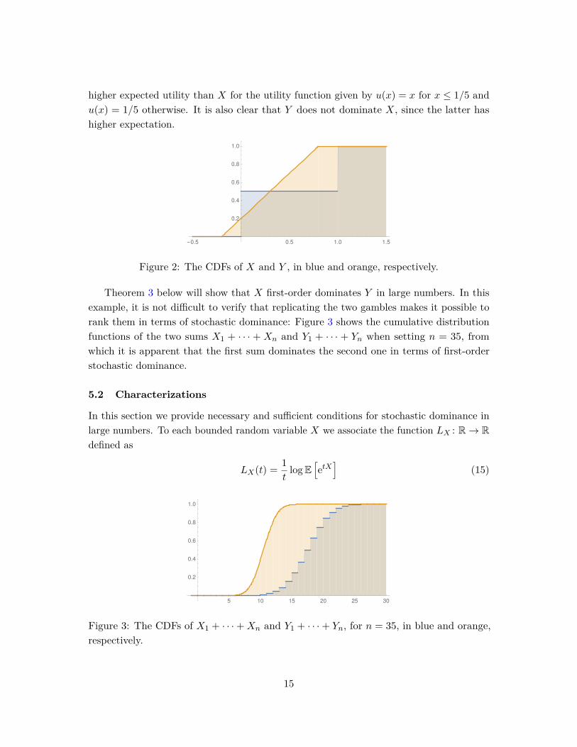
higher expected utility than X for the utility function given by u(x) = x for x ≤ 1/5 andu(x) = 1/5 otherwise. It is also clear that Y does not dominate X, since the latter hashigher expectation.
-0.5 0.5 1.0 1.5
0.2
0.4
0.6
0.8
1.0
Figure 2: The CDFs of X and Y , in blue and orange, respectively.
Theorem 3 below will show that X first-order dominates Y in large numbers. In thisexample, it is not difficult to verify that replicating the two gambles makes it possible torank them in terms of stochastic dominance: Figure 3 shows the cumulative distributionfunctions of the two sums X1 + · · · + Xn and Y1 + · · · + Yn when setting n = 35, fromwhich it is apparent that the first sum dominates the second one in terms of first-orderstochastic dominance.
5.2 Characterizations
In this section we provide necessary and sufficient conditions for stochastic dominance inlarge numbers. To each bounded random variable X we associate the function LX : R→ Rdefined as
LX(t) = 1t
logE[etX
](15)
5 10 15 20 25 30
0.2
0.4
0.6
0.8
1.0
Figure 3: The CDFs of X1 + · · ·+Xn and Y1 + · · ·+ Yn, for n = 35, in blue and orange,respectively.
15

for all t 6= 0, and, to guarantee continuity,
LX(0) = E [X]. (16)
If X is a gamble, then LX(t) is the certainty equivalent that a decision maker ascribes toX, under expected utility and a utility function u whose coefficient of absolute risk aversionis constant and equal to −t.6 Note that for t positive, such a decision maker is in factrisk-loving; we include these agents for the analysis of first-order stochastic dominance.
The quantity LX is a standard tool in the theory of choice under risk, finance, probabilitytheory, and other fields. Because it amounts to a simple normalization of the momentgenerating function of X, the certainty equivalent LX is known or can be easily computedfor most families of distributions commonly used in applications.
We similarly impose a mild genericity assumption: Say that a pair (X,Y ) is genericif min[X] 6= min[Y ] and max[X] 6= max[Y ]. The next result characterizes first-orderdominance in large numbers:
Theorem 3. Let X and Y be a generic pair of bounded random variables. Then thefollowing are equivalent:
(i). LX(t) > LY (t) for all t ∈ R,
(ii). X first-order dominates Y in large numbers.
The result is an immediate corollary of Proposition 3 introduced in the proof of Theorem1; see also Aubrun and Nechita (2008, Lemma 2). Figure 4 depicts the certainty equivalentsLX and LY for the two gambles introduced in our earlier example. As shown in the figureand can be verified analytically, the certainty equivalent of X lies above that of Y .
-20 -10 10 20
0.2
0.4
0.6
0.8
1.0
Figure 4: LX and LY in the example of §5.1, in blue and orange, respectively.6Up to an affine transformation, u is of the form u(x) = etx for t positive, u(x) = −etx for t negative
and u(x) = x for t = 0.
16

We now turn our attention to preferences that display risk aversion. The next theoremcharacterizes higher-order dominance in large numbers:
Theorem 4. Let X and Y be a generic pair of bounded random variables such thatE [X] 6= E [Y ]. Then the following are equivalent:
(i). LX(t) > LY (t) for all t ≤ 0.
(ii). X second-order dominates Y in large numbers.
(iii). X kth-order dominates Y in large numbers, for some k ≥ 2.
(iv). X ≥k Y , for some k ≥ 2.
Theorem 4 establishes a sharp equivalence between stochastic dominance in largenumbers and an elementary and well-known class of preferences. The correspondence of(i) and (ii) shows that whenever all risk averse CARA agents unanimously prefer X overY , then, for a large enough number of repetitions, all agents with monotone risk-aversepreferences will agree on this ranking. Moreover, this condition is both sufficient andnecessary.
The equivalence of (ii) and (iii) shows that there is no difference between secondand higher order risk attitudes when it comes to large numbers: For every k ≥ 2, Xkth-order dominates Y in large numbers if and only if it second-order dominates it inlarge numbers. This fact might appear surprising. Higher-order risk attitudes describeincreasingly nuanced properties of a decision maker’s preferences. Prudence (Kimball,1990), i.e. the requirement that the third derivative of the decision maker’s utility functionis positive, and temperance (Kimball, 1991), i.e. the requirement that its fourth derivative isnegative, are known to have strong implications for comparative statics in decision problemsunder risk, including precautionary saving problems and decisions under background risk(Gollier, 2004). Theorem 4 shows that when considering a sum of a sufficiently largenumber of i.i.d. gambles, the distinction between risk aversion and higher-order riskattitudes collapses.
Finally, the equivalence between (iv) and (ii) establishes a novel characterization ofhigher-order risk dominance based on the study of compound gambles: for every k ≥ 2, k-thorder stochastic dominance implies second-order stochastic dominance in large numbers,which in turn implies k-th order stochastic dominance for some k.
Next, we recall that Y is a mean preserving spread of X if both have the sameexpectation and X second-order stochastically dominates Y . We define the notion of amean preserving spread in large numbers analogously to Definition 2, so that for equal meanrandom variables it coincides with second-order stochastic dominance in large numbers.
17

Theorem 5. Let X and Y be a generic pair of bounded random variables such thatE [X] = E [Y ]. Then the following are equivalent:
(i). Var(X) < Var(Y ), LX(t) > LY (t) for all t < 0, and LX(t) < LY (t) for all t > 0.
(ii). Y is a mean preserving spread of X in large numbers.
Hence, when X and Y have the same expected value, X second-order dominates Y inlarge numbers if and only if X has lower variance and is preferred to Y by any risk-averseCARA agent, while Y is preferred to X by all CARA agents who are risk-loving.
One may wonder about the difference between condition (i) here and condition (i) inTheorem 3. Note that first-order dominance in large numbers is equivalent to LX(t) > LY (t)for all t, whereas Theorem 5 requires LX(t) to be smaller for t > 0. There is however noinconsistency, because the assumption E [X] = E [Y ] in Theorem 5 already rules out thepossibility that X1 + · · · + Xn can first-order dominate Y1 + · · · + Yn. Furthermore, inorder for X1 + · · ·+Xn to second-order dominate Y1 + · · ·+ Yn, the former sum must be amean-preserving contraction of the latter. This suggests that the right-tail of X1 + · · ·+Xn
should be less spread-out, as captured by LX(t) < LY (t) for t > 0, unlike in the case offirst-order stochastic dominance.
We conclude by observing that stochastic dominance in large numbers can be naturallyextended to compare compound i.i.d. returns. Two random returns X and Y can be rankedby requiring that for every n large enough their compounded i.i.d. returns satisfy
X1 × · · · ×Xn ≥k Y1 × · · · × Yn. (17)
The resulting stochastic order amounts to stochastic dominance in large numbers appliedto log(X) and log(Y ), and is characterized in terms of the certainty equivalents inducedby all preferences that display constant relative risk aversion.
6 Discussion and Related Literature
Comparison of Experiments. Blackwell (1951, p.101) posed the question of whetherdominance of two experiments is equivalent to dominance of their n-fold repetitions. Inthe statistics literature, Torgersen (1970) provides an early example of two experimentsthat are not comparable in the Blackwell order, but are comparable in large samples.
Moscarini and Smith (2002) produce an alternative criterion for comparing repeatedexperiments. According to their notion, an experiment P dominates an experiment Q iffor every decision problem with finitely many actions, there exists some N such that thepayoff achievable from P⊗n is higher than that from Q⊗n whenever n ≥ N . This orderis characterized by the efficiency index of an experiment, defined, in our notation, as theminimum over t ∈ (0, 1) of the function (t− 1)R0
P (t). While in Moscarini and Smith (2002)
18

the number n of repetitions is allowed to depend on the decision problem, dominance inlarge samples is a criterion for comparing experiments uniformly over decision problems,and thus is conceptually closer to Blackwell dominance.7
Azrieli (2014) shows that the Moscarini-Smith order is a strict refinement of dominancein large samples. Perhaps surprisingly, this conclusion is reversed under a modificationof their definition: When extended to consider all decision problems, including problemswith infinitely many actions, the Moscarini-Smith order over experiments coincides withdominance in large samples.8
Our notion of dominance in large samples is prior-free. In contrast, several authors(Kelly, 1956; Lindley, 1956; Cabrales, Gossner, and Serrano, 2013) have studied a completeordering of experiments, indexed by the expected reduction of entropy from prior toposterior beliefs (i.e., mutual information between states and signals). We note that unlikeBlackwell dominance, dominance in large samples does not guarantee a higher reduction ofuncertainty given any prior belief.9
Majorization and Quantum Information. Our work is related to the study of ma-jorization in the quantum information literature. Majorization is a stochastic ordercommonly defined for distributions on countable sets. For distributions with a givensupport size, this order is closely related to the Blackwell order. Let P = (Ω, P0, P1) andQ = (Ξ, Q0, Q1) be two experiments such that Ω and Ξ are finite and of the same size, andP0 and Q0 are the uniform distributions on Ω and Ξ. Then P Blackwell dominates Q ifand only if P1 majorizes Q1 (see Torgersen, 1985, p. 264). This no longer holds when Ωand Ξ are of different sizes.
Motivated by questions in quantum information, Jensen (2019) asks the followingquestion: Given two finitely supported distributions µ and ν, when does the n-fold productµ×n = µ× · · · × µ majorize ν×n for all large n? He shows that for the case that µ and νhave different support sizes, the answer is given by the ranking of their Rényi entropies.10
7Recent work by Hellman and Lehrer (2019) generalizes the Moscarini-Smith order to Markov (ratherthan i.i.d.) sequences of experiments. An interesting question for future work is whether dominance inlarge samples admits a similar generalization.
8Consider the following extension of the Moscarini-Smith order: say that P dominates Q if for everydecision problem (with possibly infinitely many actions) there exists an N such that the expected utilityachievable from P⊗n is higher than that from Q⊗n whenever n ≥ N . Each Rényi divergence RθP (t)corresponds to the indirect utility defined by a decision problem (see the proof of Theorem 1 in theappendix), and for such decision problems the ranking over repeated experiments is independent of thesample size n. We deduce that P dominates Q in this order only if P dominates Q in the Rényi order. ByTheorem 1, P must then dominate Q in large samples.
9To see this, consider the example in §3.2 with parameters α = 0.1 and β = 0. Then Proposition 2ensures that the experiment P dominates Q in large samples. However, given a uniform prior, the residualuncertainty under P is calculated as the expected entropy of posterior beliefs, which is 1
2 log(2) ≈ 0.346.The residual uncertainty under Q is −α logα− (1− α) log(1− α) ≈ 0.325, which is lower.
10As discussed above, majorization with different support sizes does not imply Blackwell dominance.
19

For the case of equal support size, our Theorem 1 implies a similar result, which Jensen(2019, Remark 3.9) conjectures to be true. We prove his conjecture in the appendix.
Fritz (2018) uses an abstract algebraic approach to prove a result that is complementaryto Theorem 3. While Fritz’s theorem does not require our genericity condition, thecomparison of distributions is stated in terms of a notion of approximate stochasticdominance. As we mentioned above, a statement similar to Theorem 3 is implied by theproof of Lemma 2 in Aubrun and Nechita (2008), also in the context of majorization andquantum information theory.
Stochastic Orders. Müller and Stoyan (2002) and Shaked and Shanthikumar (2007)are comprehensive sources on stochastic orders. The ordering generated by the functionalsof the form LX(t) for t > 0, is known in the literature as the Laplace Transform Order, andstudied in Reuter and Riedrich (1981), Fishburn (1980), Alzaid et al. (1991) and Caballéand Pomansky (1996), among others.
Hart (2011) proposes two complete stochastic orders that refine second-order stochasticdominance: wealth-uniform dominance and utility-uniform dominance. He further showsthat dominance in these orders is characterized by having a smaller riskiness index/measuregiven in Aumann and Serrano (2008) and Foster and Hart (2009), respectively. But sincethese measures of risk are distinct, an open question left by Hart (2011) is whether the twostochastic orders agree on interesting cases beyond second-order stochastic dominance. In§K, we show that the two uniform dominance orders both refine second-order dominancein large numbers.
Experiments for Many States. Our analysis leaves open a number of questions. Themost salient is the extension of Theorem 1, our characterization of dominance in largesamples, to experiments with more than two states. A natural conjecture is that the rankingof the multidimensional moment generating function of the log-likelihood ratio—whichtranslates to Rényi divergences in the two state case—characterizes this order for anynumber of states. Unfortunately, our proof technique does not straightforwardly extendto this general case. In particular, we do not know how to extend the reduction of theBlackwell order to first-order stochastic dominance (Theorem 2). The technical difficultythat arises when studying the Blackwell order for more than two states is not new to theliterature. As Jewitt (2007) writes, “the problem is the need to deal with a multivariatestochastic dominance relation for a class of functions (convex) for which the set of extremalrays is too complex to be of service.”
Indeed, the ranking based on Rényi entropies is distinct from our ranking based on Rényi divergences unlessthe support sizes are equal. See §L in the appendix for details.
20

Appendix
A Uniform Large Deviations
We begin by reviewing some standard concepts from large deviations theory. For everybounded random variable X we define ρX : R→ R+ as
ρX(a) = inft∈R
e−atMX(t).
whereMX(t) = E[etX
]is the moment generating function ofX. We note that e−atMX(t) =
MX−a(t), hence ρX(a) is the infimum of the moment generating function of X − a.We call a random variable non-degenerate if its distribution is not a point mass. In
this case, as is well known, MX is strictly log-convex, and if min[X] < a < max[X] thenMX−a(t)→∞ as |t| → ∞. It follows that for every a in the range min[X] < a < max[X]the minimization problem in the definition of ρX , which is equivalent to minimizing thestrictly convex function −at+ logMX(t), has a unique solution. We denote this minimizerby
tX(a) = argmint∈R
e−atMX(t).
LetKX(t) = logMX(t) denote the “cumulant generating function” of X. The first-ordercondition gives that tX(a) solves
K ′X(t(a)) = M ′X(t(a))MX(t(a)) = a.
Note that MX(0) = 1 and M ′X(0) = E [X]. So K ′X(0) = E [X]. This, together with theconvexity of KX , shows that t(a) ≥ 0 if and only if a ≥ E [X].
Finally, for every min[X] < a < max[X] we define
σX(a) =√M ′′X(t(a))MX(t(a)) − a
2.
Using the above formula for t(a), we also have σX(a) =√K′′X(t(a)) which is strictly
positive whenever X is non-degenerate.We will refer to quantities above as simply ρ(·), t(·) and σ(·) whenever X is unam-
biguously explicit from the context. The following technical lemma relates these functionsfor a random variable X to the corresponding functions for its negative −X; it will allowus to focus on large deviations “on one side” (of the expected value) and quickly deduceanalogous results for the other side.
21

Lemma 2. Let X be a bounded and non-degenerate random variable. Then ρ−X(a) =ρX(−a) for every a. If in addition min[X] < a < max[X] then t−X(a) = −tX(−a) andσ−X(a) = σX(−a).
Proof. Notice that MX(t) = M−X(−t). Hence, given a, we have that for every t,e−atM−X(t) = ea·(−t)MX(−t). It follows from this that ρ−X(a) = ρX(−a) and t−X(a) =−tX(−a). σ−X(a) = σX(−a) then follows from the definition.
The main technical tool of this paper is the following lemma, due, in various forms,to (Bahadur and Rao, 1960, Lemma 2) and to (Petrov, 1965, Theorems 5 and 6). It is asharp, quantitative large deviations estimate, which will be useful not only for proving ourasymptotic results above, but can also be used for estimating the number n of repetitionsrequired to achieve stochastic dominance.
Lemma 3. Let X be a bounded and non-degenerate random variable and let b > 0 satisfyP [|X| ≤ b/2] = 1. Let X1, X2, . . . be i.i.d. copies of X.
Then for every E [X] ≤ a < max[X] and every n, it holds that
P [X1 + · · ·+Xn ≥ a · n] ≤ ρ(a)n. (18)
And for every E [X] ≤ a < max[X] and n ≥ (10b/σ(a))2 it holds that
P [X1 + · · ·+Xn ≥ a · n] ≥ C(a) · ρ(a)n√n
(19)
whereC(a) = e−10t(a)b · b
σ(a) ·
Inequalities similar to (18) and (19) apply to values of a that lie below the expectationof X. Consider the case where min[X] < a ≤ E [X]. Then, by applying the inequality (19)to the random variable −X and using Lemma 2, we obtain that for every n ≥ (10b/σX(a))2,
ρX(a)n = ρ−X(−a)n ≥ P [−X1 − · · · −Xn ≥ −a · n] = P [X1 + · · ·+Xn ≤ a · n]
≥ e−10t−X(−a)b · bσ−X(−a) · ρ−X(−a)n√
n= e10tX(a)b · b
σX(a) · ρX(a)n√n
.(20)
A corollary of this lemma is a lower estimate that is uniform over a ∈ [E [X],max[X]−ε].
Corollary 1. In the setting of Lemma 3, let A = [a, a] ⊂ [E [X],max[X]) be a giveninterval. Then
CA = infa∈A
C(a) and nA = supa∈A
(10b/σ(a))2
are positive and finite, and hence for every a ∈ A and every n ≥ nA
P [X1 + · · ·+Xn ≥ a · n] ≥ CA ·ρ(a)n√n· (21)
22

Proof. Since t(a) solves K ′X(t(a)) = a and KX is strictly convex, t(a) must be strictlyincreasing in a. It is thus continuous and bounded above on the compact set A. Similarlyσ(a) is continuous and strictly positive, so it is bounded above and away from zero on A.Thus CA > 0 and nA <∞.
The next lemma is a refined version of Lemma 3, applicable to the regime of a thatvanishes with n.
Lemma 4. In the setting of Lemma 3, for every E [X] ≤ a < max[X] and every n it holdsthat
P [X1 + · · ·+Xn ≥ an] ≤ 1 +√
2π · t(a)b√2π · σ(a)t(a)
· ρ(a)n√n.
And for every E [X] ≤ a < max[X] and n ≥ 2[σ(a)t(a)]−2 it holds that
P [X1 + · · ·+Xn ≥ an] ≥ 1− 2√
2π · t(a)b2√
2π · σ(a)t(a)· ρ(a)n√
n.
This, and the previous lemma 3, are proved in the rest of this section.
A.1 Proof of Lemma 3
We follow Bahadur and Rao (1960). For each a such that E [X] ≤ a < max[X], denote
pn(a) = P [X1 + · · ·+Xn ≥ an].
Let Y a = X − a and let Fa be its cumulative distribution function. Consider, in addition,a random variable Za whose c.d.f. is given by
G(z) = 1ρ(a) ·
∫ z
−∞et(a)·y dFa(y).
Note that G(∞) = 1 because by definition MY a(t(a)) = ρ(a).More generally, the moment generating function of Za is given by
MZa(r) = MY a(r + t(a))ρ(a) = MY a(r + t(a))
MY a(t(a))
It follows from M ′Y a(t(a)) = 0 that M ′Za(0) = 0, hence Za has mean 0. Moreover
σ(a)2 = M ′′Y a(t(a)) = M ′′Za(0) = Var(Za).
It is clear that Za has the same support as Y a, which, for the entire range of values of awe consider, is contained in [−b, b]. Thus we further have
E[|Za|3
]≤ b · E
[(Za)2
]= b · σ(a)2.
23

Let Za1 , . . . , Zan be i.i.d. copies of Za, and define
Uan = Za1 + · · ·+ Zan√n · σ(a) .
Denote by Han(z) = P [Uan ≤ z] the c.d.f. of Uan . Then we can apply Lemma 2 in Bahadur
and Rao (1960) to obtain11
pn(a) = ρ(a)n ·√nσ(a)t(a) ·
∫ ∞0
e−√nσ(a)t(a)z · (Ha
n(z)−Han(0)) dz.
Clearly, Han(z)−Ha
n(0) ≤ 1 for each z. So pn(a) ≤ ρ(a)n, which yields (18), also known asthe Chernoff bound.
In the other direction, for any z0 > 0 we have
pn(a) ≥ ρ(a)n ·√nσ(a)t(a) ·
∫ ∞z0
e−√nσ(a)t(a)z · (Ha
n(z0)−Han(0)) dz
= ρ(a)n · e−√nσ(a)t(a)z0 · (Ha
n(z0)−Han(0)). (22)
By the Berry-Esseen Theorem12
Han(z0)−Ha
n(0) ≥∫ z0
0
1√2π
e−x2/2 dx− E[|Za|3
]σ(a)3√n
≥∫ z0
0
1√2π
e−x2/2 dx− b
σ(a)√n.
Note that if z0 ≤ 1 then the first term on the right hand side is at least z0/5. Hence, if wepick z0 = 10b/(σ(a)
√n), and let n0 = (10b/σ(a))2, then for all n ≥ n0 we have that z0 ≤ 1
and so the above yields Han(z0)−Ha
n(0) ≥ b/(σ(a)√n). Hence from (22) it holds for all
n ≥ n0 that
pn(a) ≥ ρ(a)n · e−√nσ(a)t(a)z0 · (Ha
n(z0)−Han(0))
≥ ρ(a)n · e−10t(a)b · b
σ(a)√n,
which shows (19).
A.2 Proof of Lemma 4
We initially proceed as in the proof of Lemma 3, arriving at
pn(a) = ρ(a)n ·√nσ(a)t(a) ·
∫ ∞0
e−√nσ(a)t(a)z · (Ha
n(z)−Han(0)) dz.
Let Φ denote the cdf of a standard Gaussian distribution. By the Berry-Esseen Theorem
Han(z)−Ha
n(0) ≤ Φ(z)− Φ(0) + b
σ(a)√n·
11The lemma follows from the definitions and integration by parts. We do not repeat the details.12In fact, to obtain a simpler expression we use some recent improvements in the estimate of the constant
in the Berry-Esseen Theorem by Tyurin (2010).
24

Hence
pn(a) ≤ ρ(a)n ·√nσ(a)t(a) ·
∫ ∞0
e−√nσ(a)t(a)z ·
(Φ(z)− Φ(0) + b
σ(a)√n
)dz.
Let c =√nσ(a)t(a). Then integration by parts implies
c
∫ ∞0
e−cz · (Φ(z)− Φ(0)) dz = ec2/2 · Φ(−c) (23)
Standard bounds for Φ assert that
1c√
2π
(1− 1
c2
)≤ ec2/2 · Φ(−c) ≤ 1
c√
2π. (24)
We thus obtain from the upper bound and (23) that
pn(a) ≤ ρ(a)n(
1√2π√nσ(a)t(a)
+ b
σ(a)√n
)
= ρ(a)n 1√2π√nσ(a)t(a)
(1 +√
2πt(a)b).
In the other direction, applying Berry-Esseen again, we have
Han(z)−Ha
n(0) ≥ Φ(z)− Φ(0)− b
σ(a)√n·
For n ≥ 2[σ(a)t(a)]−2, we have c ≥√
2, and so the lower bound in (24) implies
ec2/2Φ(−c) ≥ 12√
2πc.
It follows from this estimate and (23) that
pn(a) ≥ ρ(a)n(
12√
2π√nσ(a)t(a)
− b
σ(a)√n
)
= ρ(a)n 12√
2π√nσ(a)t(a)
(1− 2
√2πt(a)b
).
B Proof of Proposition 3 and Theorem 3
It is not difficult to see that Proposition 3 implies Theorem 3. Indeed, to prove Theorem 3we just need to show one direction, that LX(t) > LY (t) for all t (recall the definition of LXin (15) and (16)) implies X1 + · · ·+Xn dominates Y1 + · · ·+Yn for large n. By Proposition3,
P [X1 + · · ·+Xn ≥ na] ≥ P [Y1 + · · ·+ Yn ≥ na]
25

for every a ≥ E [Y ] and n ≥ N . Moreover, LX(t) > LY (t) for t ≤ 0 implies thatL−Y (t) > L−X(t) for t ≥ 0. Thus, applying Proposition 3 to the pair −Y and −X, weobtain
P [−Y1 − · · · − Yn ≥ na] ≥ P [−X1 − · · · −Xn ≥ na]
for every a ≥ E [−X] and n ≥ N . Setting a = −a, this is equivalent to
P [X1 + · · ·+Xn > na] ≥ P [Y1 + · · ·+ Yn > na]
for every a ≤ E [X]. Thus the inequality holds for all a when n is sufficiently large, andTheorem 3 holds.
To prove Proposition 3, let b be a positive number so that X and Y are supportedon [−b/2, b/2]. Without loss of generality we assume X and Y are non-degenerate.13
Moreover, since LX(t) > LY (t) for all t ≥ 0 (as this is equivalent to conditions (ii) and(iii)), letting t→∞ yields max[X] ≥ max[Y ]. Since they are unequal by assumption, wein fact have max[X] > max[Y ].
Denote by F ∗n (respectively G∗n) the c.d.f. of the sum of n i.i.d. copies ofX (respectivelyY ). We need to show 1−F ∗n(na) ≥ 1−G∗n(na) for a ≥ E [Y ] and n large. We divide theproof into cases.
Case 1: a > max[Y ]. In this case G∗n(na) = 1, and so trivially 1−F ∗n(na) ≥ 1−G∗n(na)for any n.
Case 2: E [X] ≤ a ≤ max[Y ]. Assume, without loss of generality, that max[Y ] > E [X].Let A = [E [X],max[Y ]] and consider CA, nA as defined in Corollary 1, applied to therandom variable X. When a ∈ A we have e−atMX(t) > e−atMY (t) for every t > 0.
Since for a > E [X] we have tX(a) > 0, this implies
ρX(a) = MX−a(tX(a)) > MY−a(tX(a)) ≥ ρY (a).
But even if a = E [X], it still holds that ρX(a) = 1 = MY−a(0) > ρY (a) since tY (a) > 0.Thus ρX(a) > ρY (a) whenever a ∈ A.
Now, Corollary 1 implies that for all a ∈ A and n ≥ nA,
1− F ∗n(an) ≥ CA ·ρX(a)n√
n, (25)
while Lemma 3 implies1−G∗n(an) ≤ ρY (a)n. (26)
13Otherwise, we can find non-degenerate random variables X and Y with distributions close to X and Y ,such that X dominates X and Y dominates Y in first-order stochastic dominance, and that LX(t) > LY (t)still holds for every t ≥ 0. The result of Proposition 3 for the pair X, Y implies the corresponding result forthe pair X,Y .
26

As ρX and ρY are continuous functions and ρX(a) > ρY (a) on A, the ratio ρX/ρY isbounded below by 1 + ε for some ε > 0.14
Hence, for any n such that
CA >
√n
(1 + ε)n and n ≥ nA
it follows from (25) and (26) that 1− F ∗n(an) > 1−G∗n(an) for all a ∈ A.
Case 3: E [Y ] ≤ a ≤ E [X]. By the Berry-Esseen Theorem there exist constants kX andkY such that for all a, ∣∣∣∣F ∗n(na)− Φ
(√n · a− E [X]
σX
)∣∣∣∣ ≤ kX√n
(27)∣∣∣∣G∗n(na)− Φ(√
n · a− E [Y ]σY
)∣∣∣∣ ≤ kY√n.
where Φ denotes the cdf of a standard Gaussian distribution, and σX , σY denote thestandard deviations of X and Y .
Fix a0 = 12(E [X] + E [Y ]). Since a0 > E [Y ] there exists an N such that n ≥ N implies
G∗n(na0) ≥ Φ(√
n · a0 − E [Y ]σY
)− κY√
n> 0.99− κY√
n≥ 1
2 + κX√n≥ F ∗n(n · E [X]).
where the first and the last inequalities follow directly from (27). Similarly, there exists N ′
such that n ≥ N ′ implies
F ∗n(na0) ≤ Φ(√
n · a0 − E [X]σY
)+ κX√
n< 0.01 + κX√
n≤ 1
2 −κY√n≤ G∗n(n · E [Y ]).
Hence for n ≥ maxN,N ′, if a0 ≤ a ≤ E [X], then
G∗n(na) ≥ G∗n(na0) > F ∗n(n · E [X]) ≥ F ∗n(na).
Conversely, if E [Y ] ≤ a ≤ a0 then
F ∗n(na) ≤ F ∗n(na0) < G∗n(n · E [Y ]) ≤ G∗n(na).
Therefore 1− F ∗n(na) > 1−G∗n(na) holds for all a in this range. Proposition 3 follows.14For E [X] ≤ a ≤ max[Y ], and ρY (a) = 0 if and only if a = max[Y ] and the distribution of Y has an
atom at max[Y ]. On the other hand, ρX is strictly positive on this interval.
27

C Preliminaries for Comparison of Experiments
We collect here some useful facts regarding the distributions of log-likelihood ratios inducedby an experiment. Let P = (Ω, P0, P1) be an experiment and let
Π = dP1/dP01 + dP1/dP0
be the random variable corresponding to the posterior probability that θ equals 1. Forevery A ⊆ [0, 1] we have
π1(A) =∫
Π∈AdP1 =
∫Π∈A
dP1dP0
dP0 =∫
Π∈A
Π1−Π dP0
Thus
dπ1dπ0
(p) = p
1− p. (28)
Recall that π = 12π0 + 1
2π1, sodπdπ1
(p) = 12p (29)
We also observe that for every function φ that is integrable with respect to F1, definedas in (4), ∫
Rφ(u) dF1(u) =
∫Rφ(−v)e−v dF0(v). (30)
This implies that the moment generating function of F1
MF1(u) =∫ ∞−∞
etudF1(u)
satisfiesMF1(t) = MF0(−t− 1) (31)
Hence, in particular, MF1(−1) = 1.
C.1 Proof of Lemma 1
Given an exponential distribution with support R+ and cdf H(x) = 1− e−x for all x ≥ 0,F and G can be written as
F (a) =∫ ∞
0F1(a+ u)dH(u) =
∫ ∞0
F1(a+ u)e−udu
and similarlyG(a) =
∫ ∞0
G1(a+ u)e−udu.
28

Consider the first part of the lemma. Suppose a ≥ b, then by assumption F1(a+ u) ≤G1(a+ u) for all u ≥ 0, which implies F (a) ≤ G(a).
For the second part of the lemma, we will establish the following identities:
F (a) =∫ ∞−a
F0(v)e−vdv and G(a) =∫ ∞−a
G0(v)e−vdv. (32)
Given this, the result would follow easily: If F0(a) ≤ G0(a) for all a ≥ b, then the aboveimplies F (−a) ≤ G(−a) for all a ≥ b.
We now show how (32) follows from (30). We first observe that by taking φ(u) =1(a,∞)(u) · e−u, (30) implies
F (a) = F1(a) + ea∫
(a,∞)e−udF1(u) = F1(a) + eaF0((−a)−) (33)
where F0((−a)−) denotes the left limit of F0 evaluated at −a. Moreover, taking φ to bethe indicator function of (−∞, a] implies
F1(a) =∫ ∞−a
e−vdF0(v).
Integration by parts leads to
F1(a) =∫ ∞−a
e−vdF0(v) = −eaF0((−a)−)−∫ ∞−a
F0(v)e−vdv
Hence by (33), we obtainF (a) =
∫ ∞−a
F0(v)e−vdv
as desired.
D Proof of Theorem 1
Throughout the proof, we use the notation introduced in §4.1 and §4.2 and further discussedin §C, as well as the notation related to large deviation estimates introduced in §A.
We first show that (i) implies (ii). As discussed in the main text, the comparison ofRényi divergences between two experiments is independent of the number of repetitions.Thus it suffices to show that the Rényi order refines the Blackwell order.
For t > 1, the function v1(p) = 2pt(1− p)1−t is strictly convex. Thus it is the indirectutility function induced by some decision problem. Moreover, it is straightforward to checkthat ∫ 1
0v1(p) dπ(p) = exp((t− 1)R1
P (t)),
which is a monotone transformation of the Rényi divergence. Thus, experiment P yieldshigher expected payoff in this decision problem (with indirect utility v) than Q only ifR1P (t) > R1
Q(t).
29

For t ∈ (0, 1), we consider the indirect utility function v2(p) = −2pt(1− p)1−t, which isnow convex due to the negative sign. Observe similarly that∫ 1
0v2(p) dπ(p) = − exp((t− 1)R1
P (t))
is again a monotone transformation of the Rényi divergence. So P yields higher payoff inthis decision problem only if R1
P (t) > R1Q(t).
For t = 1, we consider the indirect utility function v3(p) = 2p log( p1−p), which is strictly
convex. Since ∫ 1
0v3(p) dπ(p) = R1
P (1),
P yields higher payoff only if R1P (1) > R1
Q(1).Summarizing, the above family of decision problems show that P Blackwell-dominates
Q only if R1P (t) > R1
Q(t) for all t > 0. Since the two states are symmetric, we also haveR0P (t) > R0
Q(t) for all t > 0. This shows P dominates Q in the Rényi order.
We now show that (ii) implies (i). The assumptions that R0P (1) > R0
Q(1) and thatR1P (1) > R1
Q(1) are, in terms of the notation introduced in (5), is equivalent to
E [G0] < E [F0] and E [G1] < E [F1],
where, with slight abuse of notation, given a cdf H we denote by E [H] the expectation ofa random variable with distribution H.
Let X,X1, . . . , Xn be i.i.d. and distributed according to F1 and let Y, Y1, . . . , Yn bei.i.d. and distributed according to G1. By (12) the assumption that RθP (t) > RθQ(t) forall positive t 6= 1 is equivalent to having MX(t) > MY (t) for t > 0 and t < −1, andMX(t) < MY (t) for t ∈ (−1, 0). In particular, LX(t) > LY (t) for all t > −1.
By Theorem 2, it suffices to show that for n large,
X1 + · · ·+Xn − E ≥1 Y1 + · · ·+ Yn − E.
where E is an independent, positive, exponential random variable with density e−x. Thatis, we need to show for n large and all a ∈ R,
P [X1 + · · ·+Xn − E ≥ na] ≥ P [Y1 + · · ·+ Yn − E ≥ na] (34)
We consider a number of cases.
Case 1: a ≥ E [G1]. The random variables X and Y satisfy the conditions of Proposi-tion 3. Thus, for every n large enough and every a in this range it holds that
P [X1 + · · ·+Xn ≥ na] ≥ P [Y1 + · · ·+ Yn ≥ na]
30

Hence F ∗n1 (na) ≤ G∗n1 (na), and so the first statement of Lemma 1 applied to F ∗n1 , G∗n1implies
F ∗n(na) ≤ G∗n(na),
which implies (34).
Case 2: a ≤ −E [G0]. Here we repeat the argument of the previous case, but applied toF0 and G0, instead of F1 and G1. The hypothesis that MF1(t) < MG1(t) for all t < −1 isequivalent, by (31), to MF0(t) > MG0(t) for all t > 0. Moreover E [F0] > E [G0], and sothe same conditions that applied in the previous case apply here. Thus there exists N suchthat for n ≥ N it holds that
F ∗n0 (na) ≤ G∗n0 (na),
for every a ≥ E [G0]. Hence the second statement of Lemma 1 implies
F ∗n(na) ≤ G∗n(na)
for all a ≤ −E [G0].
Case 3: −E [G0] ≤ a ≤ E [G1]. Here we will still show (as in case 1) that
P [X1 + · · ·+Xn ≥ na] ≥ P [Y1 + · · ·+ Yn ≥ na],
which would imply the result via Lemma 1.Recall that tY (a) satisfies K ′Y (tY (a)) = a. Observe that K ′Y (0) = E [G1] ≥ a and
K ′Y (−1) = K ′G1(−1) = −K ′G0(0) = −E [G0] ≤ a.
Thus by convexity ofKY , we have tY (a) ∈ [−1, 0]. Since E [F1] > E [G1] and E [F0] > E [G0],it follows that tX(a) ∈ (−1, 0).
Denote A = [−E [G0], E [G1]]. By (20), we have for all n ≥ ( 10bmina∈A σY (a))2 and a ∈ A,
P [X1 + · · ·+Xn ≥ na] ≥ 1− ρX(a)n
andP [Y1 + · · ·+ Yn ≥ na] ≤ 1− C(a)√
nρY (a)n,
whereC(a) = e10tY (a)b · b
σY (a)is strictly positive when a ∈ A.
We now argue that ρX(a) < ρY (a) for a in this range. Indeed, since MY (t) > MX(t)for t ∈ (0, 1), and since (as is true for any distribution of a log-likelihood ratio) MX(0) =MX(−1) = MY (0) = MY (−1) = 1, we have
ρY (a) = e−atY (a) ·MY (tY (a)) ≥ e−atY (a) ·MX(tY (a)) ≥ e−atX(a) ·MX(tX(a)) = ρX(a).
31

But the first inequality holds equal only if tY (a) ∈ −1, 0, in which case the secondinequality must be strict, because tX(a) = argmint e−at ·MX(t) is strictly between −1 and0.
Therefore ρX(a) < ρY (a) for a ∈ A. By continuity,
γ := maxa∈A
ρX(a)ρY (a)
is strictly below 1. We therefore conclude that
P [X1 + · · ·+Xn ≥ na] ≥ P [Y1 + · · ·+ Yn ≥ na]
for every n large enough to satisfy
γn <mina∈AC(a)√
n.
This completes the proof.
E Proof of Proposition 1
Let p1 (resp. p3) be the essential minimum (resp. maximum) of the distribution π ofposterior beliefs induced by P . Since the support of π has at least 3 points, we can findp2 ∈ (p1, p3) such that π([p1, p2]) > π(p1) and π([p2, p3]) > π(p3).
We use this p2 to construct an experiment Q which has signal space 0, 1, and whichis a garbling of P . Specifically, if a signal realization under P leads to posterior beliefbelow p2, the garbled signal is 0. If the posterior belief under P is above p2, the garbledsignal is 1. Finally, if the posterior belief is exactly p2, we let the garbled signal be 0 or 1with equal probabilities.
Since π([p1, p2]) > π(p1), the signal realization “0” under experiment Q induces aposterior belief that is strictly bigger than p1, and smaller than p2. Likewise, the signalrealization “1” induces a belief strictly smaller than p3, and bigger than p2. Thus Pand Q form a generic pair, and the distribution τ of posterior beliefs under Q is a strictmean-preserving contraction of π. We now recall that the Rényi divergences are derivedfrom strictly convex indirect utility functions u(p) = −pt(1 − p)1−t for 0 < t < 1 andv(p) = pt(1− p)1−t for t > 1. Thus, RθP (t) > RθQ(t) for all θ ∈ 0, 1 and t > 0.
We will perturb Q to be a slightly more informative experiment Q′, such that P stilldominates Q′ in the Rényi order but not in the Blackwell order. For this, suppose thatunder Q the posterior belief equals q1 ∈ (p1, p2) with some probability λ, and equalsq2 ∈ (p2, p3) with remaining probability. Choose any small positive number ε, and let Q′
be another binary experiment inducing the posterior belief q1 − ε(1− λ) with probabilityλ, and inducing the posterior belief q2 + ελ otherwise. Such an experiment exists, becausethe expected posterior belief is unchanged. By continuity, RθP (t) > RθQ′(t) still holds when
32

ε is sufficiently small.15 Since P and Q′ also form a generic pair, Theorem 1 shows that Pdominates Q′ in large samples.
It remains to prove that P does not dominate Q′ according to Blackwell. Consider adecision problem where the prior is uniform, the set of actions is 0, 1, and payoffs aregiven by u(θ = a = 0) = p2, u(θ = a = 1) = 1− p2 and u(θ 6= a) = 0. The indirect utilityfunction is v(p) = max(1− p)p2, p(1− p2), which is piece-wise linear on [0, p2] and [p2, 1]but convex at p2. Recall that in constructing the garbling from P to Q, those posteriorbeliefs under P that are below p2 are “averaged” into the single posterior belief q1 underQ, and those above p2 are averaged into the belief q2. Thus Q achieves the same expectedutility in this decision problem as P (despite being a garbling). Nevertheless, observe thatQ′ achieves higher expected utility in this decision problem than Q.16 Hence Q′ achieveshigher expected utility than P , implying that it is not Blackwell dominated.
F Proof of Proposition 2
It is easily checked that the condition R1P (1/2) > R1
Q(1/2) reduces to√α(1− α) >
√β(1
2 − β) + 14 . (35)
Since the experiments form a generic pair, by Theorem 1, we just need to check dominancein the Rényi order. Equivalently, we need to show
(12 − β)rβ1−r + (1
2 − β)1−rβr + 12 < (1− α)rα1−r + (1− α)1−rαr, ∀0 < r < 1; (36)
(12 − β)rβ1−r + (1
2 − β)1−rβr + 12 > (1− α)rα1−r + (1− α)1−rαr, ∀r < 0 or r > 1;
(37)
β · ln( β12 − β
) + (12 − β) · ln(
12 − ββ
) > α · ln( α
1− α) + (1− α) · ln(1− αα
). (38)
To prove these, it suffices to consider the α that makes (35) hold with equality.17 Wewill show that the above inequalities hold for this particular α, except that (36) holdsequal at r = 1
2 . Let us define the following function
∆(r) := (12 − β)rβ1−r + (1
2 − β)1−rβr + 12 − (1− α)rα1−r − (1− α)1−rαr.
15Using the relation between R0P (t) and R1
P (1 − t), it suffices to show RθP (t) > RθQ′(t) for θ ∈ 0, 1and t ≥ 1/2. Fixing a large T , then by uniform continuity, RθP (t) > RθQ(t) implies RθP (t) > RθQ′(t) fort ∈ [1/2, T ] when ε is small. This also holds for t large, because as t→∞ the growth rate of the Rényidivergences are governed by the maximum of likelihood ratios, which is larger under P than under Q′.
16Formally, since q1 − ε(1− λ) < q1 < p2 and q2 + ελ > q2 > p2, it holds that
λ · v(q1 − ε(1− λ)) + (1− λ) · v(q2 + ελ) > λ · v(q1) + (1− λ) · v(q2).
17It is clear that inequalities are easier to satisfy when α increases in the range [0, 12 ].
33

When (35) holds with equality, we have ∆(0) = ∆(12) = ∆(1) = 0. Thus ∆ has roots
at 0, 1 as well as a double-root at 12 . But since ∆ is a weighted sum of 4 exponential
functions plus a constant, it has at most 4 roots (counting multiplicity).18 Hence theseare the only roots, and we deduce that the function ∆ has constant sign on each of theintervals (−∞, 0), (0, 1
2), (12 , 1), (1,∞).
Now observe that since 2β < α ≤ 12 , it holds that 1/2−β
β > 1−αα > 1. It is then easy
to check that ∆(r) → ∞ as r → ∞. Thus ∆(r) is strictly positive for r ∈ (1,∞). As∆(1) = 0, its derivative is weakly positive. But recall that we have enumerated the 4 rootsof ∆. So ∆ cannot have a double-root at r = 1, and it follows that ∆′(1) is strictly positive.Hence (38) holds.
Note that ∆′(1) > 0 and ∆(1) = 0 also implies ∆(1− ε) < 0. Thus ∆ is negative on(1
2 , 1). A symmetric argument shows that ∆ is positive on (−∞, 0) and negative on (0, 12).
Hence (36) and (37) both hold, completing the proof.
G Necessity of Genericity Assumption
Here we present examples to show that Theorem 3 and Theorem 1 do not hold withoutthe genericity assumption.
Gambles. The following is an example where LX(t) > LY (t) for all t ∈ R, but X doesnot dominate Y in large numbers because max[X] = max[Y ]. Fix any q ∈ (0, 1), andconsider
X =
10, w.p. q
2, w.p. 1−q2
0, w.p. 1−q2
; Y =
10, w.p. q
1, w.p. 2(1−q)3
−1, w.p. 1−q3
Let X be the random variable that takes values 2 and 0 with equal probabilities; notethat X is distributed as X, conditional on X 6= 10. Similarly define Y to take value 1w.p. 2/3 and value −1 w.p. 1
2 . It is easy to check that X1 + X2 first-order stochasticallydominates Y1 + Y2. As a result, LX(t) > LY (t) for all t. Since
MX(t) = q · e10t + (1− q) ·MX(t),
we conclude that LX(t) > LY (t) for all t.Nonetheless, we now show that X does not dominate Y in large numbers. For each n,
consider P [X1 + · · ·+Xn ≥ 10n− 9]. In other for this to happen, either every Xi takesvalue 10, or all but one Xi equals 10 and the remaining one equals 2. Thus
P [X1 + · · ·+Xn ≥ 10n− 9] = qn + nqn−1 · 1− q2 .
18This follows from Rolle’s theorem and an induction argument.
34

Similarly we have
P [Y1 + · · ·+ Yn ≥ 10n− 9] = qn + nqn−1 · 2(1− q)3 .
Since the latter probability is larger, X1 + · · ·+Xn does not first-order dominate Y1 + · · ·+Yn.19
Nonexistence of a Generator. The above example shows that stochastic dominancein large numbers does not admit a generator. Suppose, by way of contradiction, that V wasa family of functions φ : R→ R with the property that for all bounded random variablesX and Y , X first-order dominates Y in large numbers if and only if E [φ(X)] ≥ E [φ(Y )]for all φ ∈ V .
Let X, X, Y and Y be defined as in the previous paragraph. Since X dominates Y inlarge numbers, then it must hold that E
[φ(X)
]≥ E
[φ(Y )
]for all φ ∈ V . Hence,
E [φ(X)] = (1− q)E[φ(X)
]+ qφ(10) = (1− q)E
[φ(Y )
]+ qφ(10) ≥ E [φ(Y )],
implying that X dominates Y , a contradiction.
Experiments. Consider the experiments P and Q described in §3.2. Fix α = 14 and
β = 116 , which satisfy (35). Then by Proposition 2, P dominates Q in large samples.
But similar to the preceding example, we will perturb these two experiments by addinganother signal realization (to each experiment) which strongly indicates the true state is 1.The perturbed conditional probabilities are given below:
P :θ x0 x1 x2 x3
0 ε 116
12
716 − ε
1 100ε 716
12
116 − 100ε
Q :θ y0 y1 y2
0 ε 14
34 − ε
1 100ε 34
14 − 100ε
If ε is a small positive number, then by continuity P still dominates Q in the Rényiorder. Nonetheless, we show below that P⊗n does not Blackwell-dominate Q⊗n for any nand ε > 0.
To do this, let p := 100n−1
100n−1+1 be a threshold belief. We will show that a decision makerwhose indirect utility function is (p− p)+ strictly prefers Q⊗n to P⊗n. Indeed, it suffices tofocus on posterior beliefs p > p; that is, the likelihood-ratio should exceed 100n−1. UnderQ⊗n, this can only happen if every signal realization is y0, or all but one signal is y0 and
19Related, a slightly modification of this example shows that even if X1 + · · ·+Xn ≥1 Y1 + · · ·+ Yn forall large n, this does not imply that X1 + · · ·+Xn ≥1 X1 + · · ·+Xn−1 +Yn for all large n. Indeed, supposethat Y = 9 (instead of 10) w.p. q in this example, then Theorem 3 applies and shows that X dominates Yin large numbers, but P [X1 + · · ·+Xn ≥ 10n− 9] < P [X1 + · · ·+Xn−1 + Yn ≥ 10n− 9].
35

the remaining one is y1. Thus, in the range p > p, the posterior belief has the followingdistribution under Q⊗n:
p =
100n
100n+1 w.p. 12(100n + 1)εn
3·100n−1
3·100n−1+1 w.p. n8 (3 · 100n−1 + 1)εn−1
Similarly, under P⊗n the relevant posterior distribution is
p =
100n
100n+1 w.p. 12(100n + 1)εn
7·100n−1
7·100n−1+1 w.p. n32(7 · 100n−1 + 1)εn−1
Recall that the indirect utility function is (p − p)+. So Q⊗n yields higher expectedpayoff than P⊗n if and only if
n
8 (3·100n−1+1)εn−1·(
3 · 100n−1
3 · 100n−1 + 1 − p)>
n
32(7·100n−1+1)εn−1·(
7 · 100n−1
7 · 100n−1 + 1 − p).
That is,
4(3·100n−1+1)·(
3 · 100n−1
3 · 100n−1 + 1 −100n−1
100n−1 + 1
)> (7·100n−1+1)·
(7 · 100n−1
7 · 100n−1 + 1 −100n−1
100n−1 + 1
).
The LHS is computed to be 8·100n−1
100n−1+1 , while the RHS is 6·100n−1
100n−1+1 . Hence the above inequalityholds, and it follows that P⊗n does not Blackwell dominate Q⊗n.
H Proof of Theorem 4
(i) is equivalent to (ii). If X second-order dominates Y in large numbers, then, byconsidering risk-averse CARA utility functions, we obtain that LX(t) > LY (t) for all t < 0;the strict inequality is because these utility functions are strictly concave. By continuitywe thus have LX(0) ≥ LY (0), which implies E [X] ≥ E [Y ]. Since by assumption they areunequal, we in fact have E [X] > E [Y ]. Hence (ii) implies (i).
To show (i) implies (ii), suppose LX(t) > LY (t) for all t ≤ 0. As in the proof ofTheorem 3, We assume without loss of generality that X and Y are non-degenerate, anddenote by F ∗n (resp. G∗n) the c.d.f. of the sum of n i.i.d. copies of X (resp. Y ). Furthermore,by shifting X and Y by a constant, we can assume E [X] = µ and E [Y ] = −µ for somepositive number µ.
To prove second-order stochastic dominance, we need to show that for n large enoughand for every x ∈ R it holds that∫ x
−∞G∗n(t)− F ∗n(t) dt ≥ 0 (39)
We again consider a few cases.
36

Case 1: x ≤ 0. In this case Proposition 3 applied to the random variables −Y and −Ximplies G∗n(x) ≥ F ∗n(x) for all x ≤ nµ. Hence (39) holds too.
Case 2: x ≥ 0. Note that, as can be shown by integration by parts,∫ ∞−∞
G∗n(t)− F ∗n(t) dt = nE [X]− nE [Y ] = 2nµ
Hence ∫ x
−∞G∗n(t)− F ∗n(t) dt = 2nµ−
∫ ∞x
G∗n(t)− F ∗n(t) dt
= 2nµ−∫ ∞x
(1− F ∗n(t))− (1−G∗n(t)) dt
≥ 2nµ−∫ ∞
01− F ∗n(t) dt (40)
Now, again using integration by parts we have that∫ ∞0
1− F ∗n(t) dt = nµ+∫ 0
−∞F ∗n(t) dt
= nµ+∫ 0
nmin[X]F ∗n(t) dt ≤ nµ+ n · |min[X]| · F ∗n(0).
By the Chernoff bound (i.e., (18) in Lemma 3), F ∗n(0) ≤ ρ−X(0)n. Since ρ−X(0) < 1, forn large enough we have that the above is at most 3
2nµ. Applying this estimate to (40)yields ∫ x
−∞G∗n(t)− F ∗n(t) dt ≥ 1
2nµ
for all x ≥ 0, and we have ths shown that (i) is equivalent to (ii).(ii) is equivalent to (iii). Condition (ii) trivially implies (iii). Conversely, suppose it
holds for some n and k that X1 + · · ·+Xn ≥k Y1 + · · ·+ Yn. Since the risk-averse CARAutility function u(x) = e−tx has derivatives that alternate signs, by definition of ≥k weknow that each risk-averse CARA agent prefers X1 + · · · + Xn to Y1 + · · · + Yn. ThusLX(t) > LY (t) for all t ≤ 0. Hence (ii) follows by Theorem 4.
(i) is equivalent to (iv). This follows by applying Theorem 4 in Fishburn (1980),which shows that for bounded random variables X and Y with min[X] 6= min[Y ] andE [X] 6= E [Y ], X ≥k Y for some k ≥ 2 if and only if LX(t) > LY (t) for all t < 0.20 SinceLX(t) > LY (t) for all t < 0 holds by Theorem 4.
20In the notation used there, F,G ∈ P ∗ because X and Y are bounded, the condition G <0 F is satisfiedsince min[X] > min[Y ], and the condition µF >L µG is satisfied because E [X] > E [Y ].
37

I Proof of Theorem 5
We first show (ii) implies (i). Observe that by assumption, E [X1 + · · ·+Xn] = E [Y1 + · · ·+ Yn]for each n. Thus X1 + · · ·+Xn second-order stochastically dominates Y1 + · · ·+ Yn if andonly if the latter is a mean-preserving spread of the former. Thus, for every strictly convexfunction φ : R→ R (not necessarily increasing), it holds that
E [φ(X1 + · · ·+Xn)] < E [φ(Y1 + · · ·+ Yn)].
Choosing φ(x) = x2 and using E [X1 + · · ·+Xn] = E [Y1 + · · ·+ Yn], we deduce thatVar(X1 + · · ·+Xn) < Var(Y1 + · · ·+ Yn), and so Var(X) < Var(Y ). Moreover, choosingφ(x) = etx implies that MX(t) < MY (t) for all t 6= 0. This is equivalent to LX(t) < LY (t)for all t > 0 and LX(t) > LY (t) for all t < 0, as we desire to show.
Below we prove that (i) implies (ii). Since LX(t) < LY (t) for all t > 0, taking t→∞yields max[X] ≤ max[Y ] by continuity. But since X and Y are generic, we in fact havemax[X] < max[Y ]. Similarly we have min[X] > min[Y ]. We also assume without lossof generality that E [X] = E [Y ] = 0. Thus X and Y are bounded, zero mean randomvariables satisfying the following conditions:
(i). min[X] > min[Y ].
(ii). max[X] < max[Y ].
(iii). Var(X) < Var(Y )
(iv). MX(t) < MY (t) for all t 6= 0.
As in the proof of Theorem 3, denote by F ∗n (resp. G∗n) the c.d.f. of the sum of ni.i.d. copies of X (resp. Y ). Let b > 0 be a number such that X and Y are supported on[−b/2, b/2].
To prove (ii) we need to show that for n large enough and for every x ∈ R it holds that
W (x) :=∫ x
−∞G∗n(y)− F ∗n(y) dy ≥ 0. (41)
Since E [X] = E [Y ], integration by parts shows that W (x) = 0 for x sufficiently large.Thus we also have W (x) =
∫∞x F ∗n(y)−G∗n(y) dy. The above inequality reduces to∫ ∞
xF ∗n(t)−G∗n(t) dt ≥ 0. (42)
We will show that (42) holds for all x ≥ 0. The case of x ≤ 0 follows by applying the sameargument to −X and −Y , which also satisfy the above four conditions.
As before, we write x = na and consider a few cases.
38

Case 1: max[X] < a. In this range F ∗n = 1, and hence F ∗n ≥ G∗n point-wise.
Case 2: ε ≤ a ≤ max[X], with ε > 0 chosen in case 3 below. Note that LY (t) > LX(t)for all t > 0, so the random variables Y and X almost satisfy the assumptions of Proposition3, except that LY (0) = LX(0) (which equals their common expected value). However,since we have a ≥ ε, we can follow the analysis in the proof of Proposition 3 and deducethat ρY (a) > ρX(a) in this range. The result of Proposition 3 thus gives
1−G∗n(na) ≥ 1− F ∗n(na)
for all n large enough (depending on ε) and a ≥ ε. The integral in (42) is thus positive inthis range.
Case 3:√
12 Var(X) logn
n ≤ a ≤ ε. Define rX(a) = log ρX(a) (and rY analogously). Itfollows from Lemma 4 that
1− F ∗n(na) ≤ exp (n · rX(a)) · 1 +√
2πtX(a)b√2πσX(a)tX(a)
√n,
and that
1−G∗n(na) ≥ exp (n · rY (a)) 1− 2√
2πtY (a)b2√
2πσY (a)tY (a)√n,
provided thatn ≥ [σY (a)tY (a)]−2.
By Lemma 5 below r′X(0) = −tX(0) = 0 and
r′′X(0) = −t′X(0) = − 1K ′′X(0) = − 1
Var(X) .
Hence by Taylor expansion, we can write
rX(a) = rX(0) + r′X(0) + 12r′′X(0)a2 +O(a3) = − 1 +O(ε)
2 Var(X)
for 0 ≤ a ≤ ε; similarly for rY (a).Note that tX(0) = 0, so tX(a) = O(ε). Also, σX(0) = Std(X) (the standard deviation
of X), which implies σX(a) = (1 + O(ε)) Std(X). Moreover, t′X(0) = 1Var(X) > t′Y (0), so
tX(a) > tY (a) for 0 ≤ a ≤ ε whenever ε is sufficiently small. Plugging all of these estimatesinto the above inequality for F ∗n, we have
1− F ∗n(na) ≤ exp(−D(ε)a2n
2 Var(X)
)1
2√
2πVar(X)n · tY (a)D(ε), (43)
39

where D(ε) < 1 is a shorthand for 1−O(ε), which approaches 1 as ε→ 0.Similarly,
1−G∗n(na) ≥ exp(− a2n
2D(ε) Var(Y )
)D(ε)
2√
2πVar(Y )n · tY (a), (44)
provided that
n ≥ [σY (a)tY (a)]−2. (45)
Considering the ratio between (43) and (44), we obtain
1−G∗n(na)1− F ∗n(na) ≥ exp
(12
(D(ε)
Var(X) −1
D(ε) Var(Y )
)a2n
) Std(X)2 Std(Y ) .
Denote
VXY = 14
( 1Var(X) −
1Var(Y )
), (46)
which is positive since Var(X) < Var(Y ). We now choose ε small enough so that
12
(D(ε)
Var(X) −1
D(ε) Var(Y )
)> VXY > 0.
For this ε, it thus holds that
1−G∗n(na)1− F ∗n(na) ≥ exp
(VXY a
2n) Std(X)
2 Std(Y ) .
Since we are considering the case that a2 ≥ 12 Var(X) logn
n we have that
1−G∗n(na)1− F ∗n(na) ≥ exp
(12VXY Var(X) logn
) Std(X)2 Std(Y ) .
This is larger than one for n large enough. So we still have F ∗n(na) ≥ G∗n(na) point-wise.Lastly, we need to verify the condition (45). As we noted above, σY (0) = Std(Y ),
tY (0) = 0 and t′Y (0) = 1/Var(Y ). So for ε small enough and all a such that 12 Var(X) logn
n ≤a2 ≤ ε2 we have σY (a) = (1 +O(ε)) Std(Y ) and tY (a) = (1 +O(ε))a/Var(Y ). Hence
[σY (a)tY (a)]−2 ≤ 2 Var(Y )a2 ≤ 4 Var(Y )
Var(X)n
logn,
And so condition (45) will hold for all n sufficiently large.
40

Case 4:√
1n ≤ a ≤
√12 Var(X) logn
n . By the Berry-Esseen Theorem
F ∗n(na) ≥ 1√2π
∫ a√n/Std(X)
−∞e−x2/2 dx− k√
n
and
G∗n(na) ≤ 1√2π
∫ a√n/Std(Y )
−∞e−x2/2 dx+ k√
n,
where k is a constant depending only on the distribution of X and Y . Hence
F ∗n(na)−G∗n(na) ≥ 1√2π
∫ a√n/Std(X)
a√n/Std(Y )
e−x2/2 dx− 2k√n.
Since e−x2/2 is decreasing in this range we can lower bound the integrand by its right limit,yielding
F ∗n(na)−G∗n(na) ≥( 1
Std(X) −1
Std(Y )
)a√n · e−a2n/(2 Var(X)) − 2k√
n. (47)
Applying the assumption 1n ≤ a
2 ≤ 12 Var(X) logn
n yields
F ∗n(na)−G∗n(na) ≥( 1
Std(X) −1
Std(Y )
)n−1/4 − 2k · n−1/2, (48)
which is again positive for all n large enough.
Case 5: 0 ≤ a ≤√
1n . Recall that we defined
W (x) =∫ ∞x
F ∗n(y)−G∗n(y) dy.
From cases 1-4, we have shown that for y ≥√n, F ∗n(y)−G∗n(y) ≥ 0 point-wise. Moreover,
from (48) we in fact haveF ∗n(y)−G∗n(y) ≥ cn−1/4
for n large enough and√n ≤ y ≤
√12 Var(X)n logn, where c is a positive constant
independent of n. Integrating this estimate over the range of y to which it applies, wededuce
W (√n) ≥
∫ √ 12 Var(X)n logn
√n
F ∗n(y)−G∗n(y) dy = cn1/4.
On the other hand, for y ∈ [0,√n], it follows from 47 that
F ∗(x)−G∗n(x) ≥ − 2k√n.
41

So for any x ∈ [0,√n],
W (x) =∫ ∞x
F ∗n(y)−G∗n(y) dt
=∫ √nx
F ∗n(y)−G∗n(y) dy +W (√n)
≥ − 2k√n
√n+W (
√n)
= −2k + cn1/4
which is positive for n large enough. This completes the proof that W (x) ≥ 0 for all x ≥ 0,and the theorem follows.
I.1 Additional Lemma
Lemma 5. Let X be a bounded, zero mean random variable, and define rX(a) = log ρX(a).Then r′X(0) = −tX(0) = 0 and r′′X(0) = −t′X(0) = −1/Var(X).
Proof. We suppress the subscript X in this proof. Observe that r(a) = inftK(t)− at. Soby the envelope theorem, r′(a) = −t(a). Since t(E [X]) = 0, we deduce r′(0) = −t(0) = 0.
Moreover, we have r′′(a) = −t′(a). Now recall that t(a) satisfies K ′(t(a)) = a, and sot′(a) = 1
K′′(t(a)) . But from K(t) = logE[etX
]it is easy to deduce K ′′(0) = Var(X). Hence
r′′X(0) = −t′X(0) = −1/Var(X) as desired.
J Stochastic Dominance implies Dominance in Large Numbers
Lemma 6. Suppose X ≥k Y for some k ≥ 1. Then for each n and i.i.d. replicas X1, . . . , Xn
of X and Y1, . . . , Yn of Y , it holds that
X1 + · · ·+Xn ≥k Y1 + · · ·+ Yn.
Proof. We first show that if X ≥k Y , then X + Z ≥k Y + Z whenever Z is independentof both X and Y . Indeed, by definition we need to show E [u(X + Z)] ≥ E [u(Y + Z)] forany u whose first k derivatives have alternating signs. The assumption that X ≥k Y showsE [u(X + z)] ≥ E [u(Y + z)] for every realization z, since u(· + z) also has k derivativesthat alternate signs. Integrating over z then yields the claim. Repeatedly applying thisresult, we obtain
X1+· · ·+Xn ≥k X1+· · ·+Xn−1+Yn ≥k X1+· · ·+Xn−2+Yn−1+Yn ≥k · · · ≥k Y1+· · ·+Yn.
This proves the lemma.
42

K Connection to Other Stochastic Orders
Aumann and Serrano (2008) and Foster and Hart (2009) propose two criteria for measuringthe riskiness of a gamble. They focus on random variables X with E [X] > 0 andP [X < 0] > 0. The Aumann-Serrano riskiness index is the unique positive number RAS(X)such that
E[e− XRAS(X)
]= 1.
On the other hand, the Foster-Hart measure of riskiness is the unique positive numberRFH(X) such that
E[log
(1 + X
RFH(X)
)]= 0.
Hart (2011) recognizes that these indices induce two complete orderings over gamblesthat refine second-order stochastic dominance. That is, we can define X to dominateY if and only if RAS(X) ≤ RAS(Y ) (or RFH(X) ≤ RFH(Y ), respectively). He providesbehavioral characterizations of these orders, which are called “uniform-wealth dominance”and “uniform-utility dominance.”
In what follows, we show that if LX(t) ≥ LY (t) for all t ≤ 0, then X is less risky thanY according to both Aumann-Serrano and Foster-Hart. This, together with one directionof Theorem 4, then proves that the two uniform dominance orders in Hart (2011) bothrefine our second-order in large numbers dominance order.
To show RAS(X) ≤ RAS(Y ), let a denote 1RAS(X) and b denote 1
RAS(Y ) . By definitionwe have MX(−a) = 1. But since LX(−a) ≥ LY (−a) by assumption, we obtain MY (−a) ≥MX(−a) = 1. From MY (−a) ≥ 1, MY (0) = MY (−b) = 1, and the strict convexity ofMY (t), we can conclude that b ≤ a. Thus
RAS(X) = 1/a ≤ 1/b = RAS(Y ).
To show RFH(X) ≤ RFH(Y ), we similarly denote c = 1RFH(X) and d = 1
RFH(Y ) . Bydefinition,
E [log(1 + cX)] = 0 = E [log(1 + dY )].
Consider the utility function u(x) = log(1 + dx). Observe that for x > −1d , u(x) has
derivatives that alternate signs. By Bernstein’s theorem, u(x) can be written as a mixtureof linear functions and exponential functions −e−tx0≤t≤∞. Since by assumptionMX(t) ≤MY (t) for all t ≤ 0, we deduce that E [u(X)] ≥ E [u(Y )].21 In other words,
E [log(1 + dX)] ≥ E [log(1 + dY )] = 0.21Note that LX(t) ≥ LY (t) for t → −∞ implies min[X] ≥ min[Y ]. Thus whenever E [log(1 + dY )] is
defined, so is E [log(1 + dX)].
43

Now observe that the function g(λ) = E [log(1 + λX)] is strictly concave in λ, and g(0) =g(c) = 0 ≤ g(d). Hence d ≤ c. It follows that
RFH(X) = 1/c ≤ 1/d = RFH(Y ).
L Proof of a Conjecture Regarding Majorization
Jensen (2019) studies the majorization order on finitely supported distributions. Giventwo such distributions µ and ν, µ is said to majorize ν if for every n ≥ 1 it holds that thesum of the largest n probabilities in µ is greater than or equal to the sum of the n largestprobabilities in ν. The Rényi entropy of a distribution µ defined on a finite set S is givenby
Hµ(α) = 11− α log
(∑s∈S
µ(s)α),
for α ∈ [0,∞) \ 1. As with our definition of Rényi divergences, this definition is extendedto α = 1 by continuity to equal the Shannon entropy, and extended to α = ∞ to equal− log maxs µ(s). Hence Hµ is defined on [0,∞].
Note that Hµ(0) is the size of the support of µ. In his Proposition 3.7, Jensen showsthat if Hµ(α) < Hν(α) for all α ∈ [0,∞] then the n-fold product µ×n majorizes ν×n.
Commenting on his Proposition 3.7, Jensen writes “The author cautiously conjecturesthat . . . the requirement of a sharp inequality at 0 could be replaced by a similar conditionregarding the α-Rényi entropies for negative α.”
To understand this statement in terms of the nomenclature and notation of our paper,we identify each distribution µ whose support is a finite set S with the experimentPµ = (S, P1, P0), where P1 = µ and P0 is the uniform distribution on S. There is a simpleconnection between the Rényi entropy of µ and the Rényi divergence of Pµ. For α ≥ 0,
Hµ(α) = log |S| −R1P (α). (49)
As Jensen suggests, Hµ(α) for negative α is also important, as it relates to R0P . For α ≤ 0,
Hµ(α) = log |S| − α
1− αR0P (1− α), (50)
which extends to α = −∞ to equal − log mins µ(s). Moreover, note that
H ′µ(0) = −R0P (1) = log |S|+ 1
|S|∑s∈S
logµ(s). (51)
As shown by Torgersen (1985, p. 264), when µ and ν have the same support size, thenmajorization of ν by µ is equivalent to Blackwell domination of P ν by Pµ. Thus Jensen’sProposition 3.7, which assumes that the support sizes are different, has no implications forBlackwell dominance. However, our result on Blackwell dominance does have implicationsfor majorization. In particular, the following proposition follows immediately from theapplication of Theorem 1 to experiments of the form Pµ.
44

Proposition 4. Let µ, ν be finitely supported distributions with the same support size (i.e.,Hµ(0) = Hν(0)), and such that Hµ(∞) 6= Hν(∞) and Hµ(−∞) 6= Hν(−∞). Then thefollowing are equivalent:
(i). Hµ(α) < Hν(α) for all α ∈ (0,∞], Hµ(α) > Hν(α) for all α ∈ [−∞, 0) andH ′µ(0) < H ′ν(0).22
(ii). There exists an N such that µ×n majorizes ν×n for every n ≥ N .
Proof. For notational ease, let P denote Pµ and Q denote P ν . The assumption Hµ(α) <Hν(α) for all α > 0 is equivalent, via (49), to R1
P (t) > R1Q(t) for all t > 0, and to
R0P (t) > R0
Q(t) for all t ∈ (0, 1), using R0P (t) = t
1−tR1P (1− t) for 0 < t < 1.
On the other hand, Hµ(α) > Hν(α) for all α < 0 and H ′µ(0) < H ′ν(0) is equivalent, via(50) and (51), to R0
P (t) > R0Q(t) for all t ≥ 1. So (i) is equivalent to P dominating Q in
the Rényi order.Finally, the assumptions that Hµ(∞) 6= Hν(∞) and Hµ(−∞) 6= Hν(−∞) translate
into maxs µ(s) 6= maxs ν(s) and mins µ(s) 6= mins ν(s), which are in turn equivalent torequiring that P and Q be a generic pair. Therefore, by Theorem 1, (i) is equivalent toP⊗n Blackwell dominates Q⊗n for every large n. It follows from Torgersen (1985) that (i)is equivalent to (ii).
References
A. Alzaid, J. S. Kim, and F. Proschan. Laplace ordering and its applications. Journal ofApplied Probability, 28(1):116–130, 1991.
G. Aubrun and I. Nechita. Catalytic majorization and `p norms. Communications inMathematical Physics, 278(1):133–144, 2008.
R. J. Aumann and R. Serrano. An economic index of riskiness. Journal of PoliticalEconomy, 116(5):810–836, 2008.
Y. Azrieli. Comment on “the law of large demand for information”. Econometrica, 82(1):415–423, 2014.
R. R. Bahadur and R. R. Rao. On deviations of the sample mean. Ann. Math. Statist, 31(4):1015–1027, 1960.
S. Benartzi and R. H. Thaler. Risk aversion or myopia? choices in repeated gambles andretirement investments. Management science, 45(3):364–381, 1999.
22This last condition is necessary for majorization, but it was not recognized in the original conjecture ofJensen (2019).
45

D. Blackwell. Comparison of experiments. In Proceedings of the Second Berkeley Symposiumon Mathematical Statistics and Probability, pages 93—102. University of California Press,1951.
D. Blackwell. Equivalent comparisons of experiments. The Annals of MathematicalStatistics, pages 265–272, 1953.
D. A. Blackwell and M. A. Girshick. Theory of games and statistical decisions. CourierCorporation, 1979.
H. F. Bohnenblust, L. S. Shapley, and S. Sherman. Reconnaissance in game theory. 1949.
J. Caballé and A. Pomansky. Mixed risk aversion. Journal of economic theory, 71(2):485–513, 1996.
A. Cabrales, O. Gossner, and R. Serrano. Entropy and the value of information for investors.American Economic Review, 103(1):360–377, 2013.
H. Cramér. Sur un nouveau théoreme-limite de la théorie des probabilités. Actual. Sci.Ind., 736:5–23, 1938.
I. Csiszár. Axiomatic characterizations of information measures. Entropy, 10(3):261–273,2008.
P. C. Fishburn. Continua of stochastic dominance relations for unbounded probabilitydistributions. Journal of Mathematical Economics, 7(3):271–285, 1980.
D. P. Foster and S. Hart. An operational measure of riskiness. Journal of Political Economy,117(5):785–814, 2009.
T. Fritz. Resource convertibility and ordered commutative monoids. Mathematical Struc-tures in Computer Science, 27(6):850–938, 2017.
T. Fritz. A generalization of Strassen’s Positivstellensatz and its application to largedeviation theory. arXiv preprint arXiv:1810.08667v3, 2018.
C. Gollier. Repeated optional gambles and risk aversion. Management Science, 42(11):1524–1530, 1996.
C. Gollier. The economics of risk and time. MIT press, 2004.
S. Hart. Comparing risks by acceptance and rejection. Journal of Political Economy, 119(4):617–638, 2011.
Z. Hellman and E. Lehrer. Valuing information by repeated markov signals. WorkingPaper, 2019.
46

R. Horodecki, P. Horodecki, M. Horodecki, and K. Horodecki. Quantum entanglement.Reviews of modern physics, 81(2):865, 2009.
A. K. Jensen. Asymptotic majorization of finite probability distributions. IEEE Transac-tions on Information Theory, 2019.
I. Jewitt. Information order in decision and agency problems. Technical report, NuffieldCollege, 2007.
J. L. Kelly. A new interpretation of information rate. IRE Transactions on InformationTheory, 2(3):185–189, 1956.
M. S. Kimball. Precautionary saving in the small and in the large. Econometrica, 58(1):53–73, 1990.
M. S. Kimball. Precautionary motives for holding assets. Technical report, National Bureauof Economic Research, 1991.
M. S. Kimball. Standard risk aversion. Econometrica, pages 589–611, 1993.
A. Krishnamurthy, K. Kandasamy, B. Poczos, and L. Wasserman. Nonparametric estimationof renyi divergence and friends. In International Conference on Machine Learning, pages919–927, 2014.
F. Liese and I. Vajda. On divergences and informations in statistics and information theory.IEEE Transactions on Information Theory, 52(10):4394–4412, 2006.
D. V. Lindley. On a measure of the information provided by an experiment. The Annalsof Mathematical Statistics, 27(4):986–1005, 1956.
G. Moscarini and L. Smith. The law of large demand for information. Econometrica, 70(6):2351–2366, 2002.
A. Müller and D. Stoyan. Comparison methods for stochastic models and risks, volume389. Wiley New York, 2002.
V. V. Petrov. On the probabilities of large deviations for sums of independent randomvariables. Theory of Probability & Its Applications, 10(2):287–298, 1965.
B. Póczos, L. Xiong, and J. Schneider. Nonparametric divergence estimation with applica-tions to machine learning on distributions. arXiv preprint arXiv:1202.3758, 2012.
L. Pomatto, P. Strack, and O. Tamuz. Stochastic dominance under independent noise.arXiv preprint arXiv:1807.06927, 2019.
47

J. W. Pratt and R. J. Zeckhauser. Proper risk aversion. Econometrica, pages 143–154,1987.
M. Rabin and R. H. Thaler. Anomalies: risk aversion. Journal of Economic perspectives,15(1):219–232, 2001.
A. Rényi. On measures of entropy and information. In Proceedings of the Fourth BerkeleySymposium on Mathematical Statistics and Probability, Volume 1: Contributions to theTheory of Statistics. The Regents of the University of California, 1961.
H. Reuter and T. Riedrich. On maximal sets of functions compatible with a partial orderingfor distribution functions. Mathematische Operationsforschung und Statistik. SeriesOptimization, 12(4):597–605, 1981.
S. A. Ross. Adding risks: Samuelson’s fallacy of large numbers revisited. Journal ofFinancial and Quantitative Analysis, 34(3):323–339, 1999.
P. A. Samuelson. Risk and uncertainty: A fallacy of large numbers. Scientia, 1963.
M. Shaked and J. G. Shanthikumar. Stochastic orders. Springer Science & Business Media,2007.
L. Smith and P. Sørensen. Pathological outcomes of observational learning. Econometrica,68(2):371–398, 2000. ISSN 1468-0262.
E. Torgersen. Majorization and approximate majorization for families of measures, appli-cations to local comparison of experiments and the theory of majorization of vectors in rn (schur convexity). In Linear Statistical Inference, pages 259–310. Springer, 1985.
E. Torgersen. Comparison of statistical experiments, volume 36. Cambridge UniversityPress, 1991.
E. N. Torgersen. Comparison of experiments when the parameter space is finite. ProbabilityTheory and Related Fields, 16(3):219–249, 1970.
I. S. Tyurin. An improvement of upper estimates of the constants in the Lyapunov theorem.Russian Mathematical Surveys, 65(3):201–202, 2010.
48