BlackHolesIVU - TU Wienquark.itp.tuwien.ac.at/~grumil/pdf/BHLectureNotes.pdf · BlackHolesIVU Lecture notes written by Stefan Prohazka, Max Riegler and Sebastian Singer Supervised

Black Holes I VU

Lecture notes written byStefan Prohazka, Max Riegler and Sebastian Singer

Supervised by Daniel GrumillerWS 2009/10

Version 0.0 prepared by Daniel Grumiller and Stefan ProhazkaJanuary 26, 2016

Preliminary version – January 26, 2016

Contents

1. Historical Overview 5

2. Gravitational Collapse – Chandrasekhar Limit 72.1. Chandrasekhar Limit . . . . . . . . . . . . . . . . . . . . . . . . . . . . . . . 7

3. Phenomenology of and Experiments with Black Holes 93.1. “Fishy” Gedankenexperiment . . . . . . . . . . . . . . . . . . . . . . . . . . 93.2. Brief Review of Special Relativity . . . . . . . . . . . . . . . . . . . . . . . . 103.3. Mathematical Aspects of Special Relativity . . . . . . . . . . . . . . . . . . 12

4. Metric and Geodesic Equation 134.1. Euclidean Coordinate Transformation . . . . . . . . . . . . . . . . . . . . . 134.2. The Geodesic Equation . . . . . . . . . . . . . . . . . . . . . . . . . . . . . 14

4.2.1. Geodesics in Euclidean Space . . . . . . . . . . . . . . . . . . . . . . 144.2.2. Timelike Geodesics . . . . . . . . . . . . . . . . . . . . . . . . . . . . 154.2.3. Geodesics in a Special Metric: The Newton Limit . . . . . . . . . . . 164.2.4. General Geodesics . . . . . . . . . . . . . . . . . . . . . . . . . . . . 17

5. Geodesics for Schwarzschild Black Holes 185.1. Schwarzschild Solution: Asymptotic Behavior, Light in Radial Motion . . . 185.2. Gravitational Redshift (equivalence principle) . . . . . . . . . . . . . . . . . 195.3. Geodesic Equation of the Schwarzschild Solution . . . . . . . . . . . . . . . 20

5.3.1. Timelike Geodesic . . . . . . . . . . . . . . . . . . . . . . . . . . . . 215.3.2. Lightlike Geodesic . . . . . . . . . . . . . . . . . . . . . . . . . . . . 22

5.4. Orbits of the Schwarzschild Black Hole . . . . . . . . . . . . . . . . . . . . . 225.5. Perihelion shift . . . . . . . . . . . . . . . . . . . . . . . . . . . . . . . . . . 235.6. Gravitational Light Bending . . . . . . . . . . . . . . . . . . . . . . . . . . . 24

6. Curvature and Basics of Differential Geometry 286.1. Manifolds and Tangent Spaces . . . . . . . . . . . . . . . . . . . . . . . . . 286.2. Tensors . . . . . . . . . . . . . . . . . . . . . . . . . . . . . . . . . . . . . . 306.3. Another View at the Metric . . . . . . . . . . . . . . . . . . . . . . . . . . . 316.4. Covariant Derivatives . . . . . . . . . . . . . . . . . . . . . . . . . . . . . . 32

6.4.1. Properties of the Covariant Derivative . . . . . . . . . . . . . . . . . 336.5. Covariant Derivative acting on Dual Vectors . . . . . . . . . . . . . . . . . . 346.6. Parallel Transport . . . . . . . . . . . . . . . . . . . . . . . . . . . . . . . . 356.7. Fixing Γ Uniquely . . . . . . . . . . . . . . . . . . . . . . . . . . . . . . . . 366.8. The Riemann-Tensor . . . . . . . . . . . . . . . . . . . . . . . . . . . . . . . 37

6.8.1. Properties of the Riemann-Tensor . . . . . . . . . . . . . . . . . . . 376.9. Jacobi / Bianchi Identity . . . . . . . . . . . . . . . . . . . . . . . . . . . . 386.10. Lie Derivatives . . . . . . . . . . . . . . . . . . . . . . . . . . . . . . . . . . 396.11. Killing Vectors . . . . . . . . . . . . . . . . . . . . . . . . . . . . . . . . . . 406.12. Tensor Densities . . . . . . . . . . . . . . . . . . . . . . . . . . . . . . . . . 40

6.12.1. The Levi-Civita Symbol as a Tensor Density . . . . . . . . . . . . . 41

7. Hilbert Action and Einstein Field Equations 437.1. The Action Integral in QED . . . . . . . . . . . . . . . . . . . . . . . . . . . 437.2. Hilbert Action . . . . . . . . . . . . . . . . . . . . . . . . . . . . . . . . . . 447.3. Einstein Field Equations . . . . . . . . . . . . . . . . . . . . . . . . . . . . . 44


8. Spherically Symmetric Black Holes and the Birkhoff Theorem 468.1. Birkhoff’s Theorem . . . . . . . . . . . . . . . . . . . . . . . . . . . . . . . . 468.2. Killing vectors . . . . . . . . . . . . . . . . . . . . . . . . . . . . . . . . . . 48

8.2.1. Spacetime Singularity . . . . . . . . . . . . . . . . . . . . . . . . . . 508.2.2. Near horizon region of Schwarzschild geometry . . . . . . . . . . . . 508.2.3. Global coordinates of the Schwarzschild geometry . . . . . . . . . . . 52

8.3. Zeroth law of black hole mechanics . . . . . . . . . . . . . . . . . . . . . . . 558.4. Komar mass . . . . . . . . . . . . . . . . . . . . . . . . . . . . . . . . . . . . 56

9. Rotating Black Holes: The Kerr Solution 589.1. Uniqueness Theorem . . . . . . . . . . . . . . . . . . . . . . . . . . . . . . . 599.2. No-hair Theorem . . . . . . . . . . . . . . . . . . . . . . . . . . . . . . . . . 599.3. The Ergosphere . . . . . . . . . . . . . . . . . . . . . . . . . . . . . . . . . . 599.4. The Penrose Process . . . . . . . . . . . . . . . . . . . . . . . . . . . . . . . 609.5. Frame-dragging/Thirring-Lense Effect [gravimagnetism] . . . . . . . . . . . 60

10.Geodesics for Kerr Black Holes 6310.1. Geodesic Equation of the Kerr Black Hole . . . . . . . . . . . . . . . . . . . 6310.2. ISCO of the Kerr Black Hole . . . . . . . . . . . . . . . . . . . . . . . . . . 64

11.Accretion Discs and Black Hole Observations 6611.1. Simple Theoretical Model: General Relativistic Perfect Fluid . . . . . . . . 67

12.Black hole analogs in condensed matter physics 6912.1. Analogy theorem . . . . . . . . . . . . . . . . . . . . . . . . . . . . . . . . . 6912.2. Proof . . . . . . . . . . . . . . . . . . . . . . . . . . . . . . . . . . . . . . . . 7012.3. General remaks . . . . . . . . . . . . . . . . . . . . . . . . . . . . . . . . . . 7212.4. Example: Vortex geometry . . . . . . . . . . . . . . . . . . . . . . . . . . . 72

A. Useful formulas 75


4

PrefaceThese lecture notes were written as part of three student projects at TU Wien (by Ste-fan Prohazka, Max Riegler and Sebastian Singer, supervised by Daniel Grumiller) in2009/2010. The current version 0.0 was edited by Stefan Prohazka and corrected byDaniel Grumiller. However, the authors would be surprised if this first public version wasfree of mistakes.If you find typos or errors please contact [email protected].

Note on unitsIf not noted otherwise this script will use natural units (also known as Planck units) wherewe set human conversion factors equal to one, i.e. c = ~ = GN = kB = 1, where c is thespeed of light (Einstein’s constant), ~ is Planck’s constant, GN is Newton’s constant andkB is Boltzmann’s constant.Note that this is not neglecting anything, it just amounts to a more convenient choice of

units than the historically grown ones. c = 1 means we measure time in the same units asdistances; ~ = 1 means we measure additionally energy in inverse units of time; GN = 1then means that we set the Planck mass (and thus Planck length and Planck time) tounity and measure everything else in Planck units; kB = 1 means we measure informationin e-bits and that energy and temperature have the same units. For an enjoyable paperon dimensionfull and dimensionless constants see http://arxiv.org/abs/1412.2040 (it isinteresting to note how many well-known physicists appear to be confused about units).

Further readingInformation about running lectures by Daniel Grumiller and additional resources can befound at the teaching webpage http://quark.itp.tuwien.ac.at/ grumil/teaching.shtml.Here is further selected literature:

• Einstein gravity in a nutshell, (A. Zee, 2013, Princeton U. Press)

• Spacetime and Geometry: An Introduction to General Relativity, (S. Carroll, 2003,Addison Wesley)

• Gravitation und Kosmologie, (R.U. Sexl and H.K. Urbantke, 1987, Wissenschaftsver-lag, Mannheim/Wien/Zürich)

• General Relativity, (R. Wald, 1984, U. Chicago Press, Chicago)

• Gravitation and Cosmology: Principles and Applications of the General Theory ofRelativity (S. Weinberg, 1972, John Wiley)

• The large scale structure of space-time, (S.W. Hawking and G.F.R. Ellis, 1973,Cambridge University Press, Cambridge)

• Accretion Power in Astrophysics (J. Frank, A. King and D. Raine, 2002, CambridgeUniversity Press, Cambridge)

• Active galactic nuclei: from the central black hole to the galactic environment (J.Krolik, 1998, Princeton University Press, Princeton)

• Black Hole Physics: Basic Concepts and New Developments (V.P. Frolov and I.D.Novikov, 1998, Springer, New York)

• Gravitation, (C. Misner, K.S. Thorne and J.A. Wheeler, 1973)


mailto:[email protected]

http://arxiv.org/abs/1412.2040

http://quark.itp.tuwien.ac.at/~grumil/teaching.shtml

5

1. Historical OverviewAs an introduction to black hole physics we want to start our lecture notes by a briefhistorical overview on black hole science.

• O.C. Rømer (1676): the speed of light is finite

• I. Newton (1686): the law of gravity

Fr = −GNmM

r2 (1.1)

• J. Michell (1783): referring to Newtonian black holes, “All light emitted fromsuch a body would be made to return towards it by its own proper gravity”

• P.S. Laplace (1796): “Exposition du systéme du Monde” (“dark stars”)

• T. Young (1801): interference experiments confirm Huygens’ theory of the wavenature of light; Newton’s theory of light is dead, and so are dark stars

• A. Einstein (1905): Special Relativity

• A. Einstein (1915): General Relativity (GR)

• K. Schwarzschild (1916): first exact solution of GR is a black hole!

• S. Chandrasekhar (1931): gravitational collapse of Fermi gas

• A. Eddington (1935): regarded the idea of black holes with skepticism, “I thinkthere should be a law of Nature to prevent a star from behaving in this absurd way!”

• M. Kruskal; G. Szekeres (1960): global structure of Schwarzschild spacetime

• R. Kerr (1963): exact (and essentially unique) rotating (and charged) black holesolution sparks interest of astrophysics community

• Cygnus X-1 (1964): first detection of X-ray emission from a black hole in a binarysystem (though realized only in 1970ties that it might be black hole; conclusiveevidence only in 1990ies)

• J. Wheeler (December 1967): invention of the term “black hole”

• S. Hawking and R. Penrose (1970): black holes contain singularities

• J. Bekenstein (1972): speculation that black holes might have entropy

• N.I. Shakura and R.A. Sunyaev (1972): first accretion disk model

• J. Bardeen, B. Carter and S. Hawking (1973): four laws of black hole me-chanics

• S. Hawking (1974): black holes evaporate due to quantum effects

• W. Unruh (1981): black hole analogs in condensed matter physics

• S. Deser, R. Jackiw, C. Teitelboim et al. (1982): gravity in lower dimensions

• E. Witten et al. (1984): first superstring revolution


6 1. Historical Overview

• H.-P. Nollert; N. Andersson (1992): quasinormal modes of a “ringing” Schwarzschildblack hole

• M. Bañados, C. Teitelboim and J. Zanelli (1992): black holes in 2 + 1 dimen-sions

• M. Choptuik (1993): Critical collapse in numerical relativity discovered

• G. ’t Hooft and L. Susskind (1993): holographic principle

• M. Veltman (1994): black holes still sometimes regarded with skepticism, “Blackholes are probably nothing else but commercially viable figments of the imagination.”

• J. Polchinski (1995): p-branes and second superstring revolution

• A. Strominger and C. Vafa (1996): microscopic origin of black hole entropy

• J. Maldacena (1997): AdS/CFT correspondence

• S. Dimopoulos and G.L. Landsberg; S.B. Giddings and S. Thomas (2001):black holes at the LHC?

• Saggitarius A∗ (2002): supermassive black hole in center of Milky Way

• R. Emparan and H. Reall (2002): black rings in five dimensions

• G. ‘t Hooft (2004): “It is however easy to see that such a position is untenable.”(comment on Veltman a decade earlier)

• S. Hawking (2004): concedes bet on information paradox; end of “black holewars”

• P. Kovtun, D. Son and A. Starinets (2004): viscosity in strongly interactingquantum field theories from black hole physics

• F. Pretorius (2005): breakthrough in numerical treatment of binary problem

• C. Barcelo, S. Liberati, and M. Visser (2005): “Analogue gravity” - blackhole analogon in condensed matter physics

• J.E. McClintock et al. (2006): measuring of spin of GRS1915+105 – nearlyextremal Kerr black hole!

• E. Witten (2007) and W. Li, W. Song and A. Strominger (2008): quantumgravity in three dimensions?

• S. Hughes (2008): “Unambiguous observational evidence for the existence of blackholes has not yet been established.”

• S. Hughes (2008): “Most physicists and astrophysicists accept the hypothesis thatthe most massive, compact objects seen in many astrophysical systems are describedby the black hole solutions of general relativity.”

• S. Gubser; S. Hartnoll, C. Herzog and G. Horowitz (2008): “holographicsuperconductors”

• D. Son; K. Balasubramanian and J. McGreevy (2008): black hole duals forcold atoms proposed

More recent developments are not included in this list, but will be updated in the listpresented in the first lectures of “Black holes I”.


7

2. Gravitational Collapse – Chandrasekhar Limit

Four fundamental interactions are known to physicists today - gravitational, electromag-netic, strong and weak interaction.On large (cosmological) scales, only gravity – the weakest of these forces – plays a majorrole. This is easily understood by the facts that the nuclear forces are extremely shortranged (about the radius of nuclei) and that our Universe is electrically neutral on largescales.

During the history of the Universe it was gravity that intensified local density fluctua-tions. This process finally led to the formation of planets, stars, galaxies and even blackholes.

So, in order to understand the formation of a black hole, we must investigate the influ-ence of gravity in stellar dynamics. Accordingly, the aim of this chapter will be to deriveapproximate stability limits for stars.

2.1. Chandrasekhar Limit

As long as a star can fusion lighter elements into more heavy ones, the thermal and ra-diation outward pressure counteracts gravitational collapse. Only when the end of stellarfusion is reached, gravitational collapse can begin. This process continues until all energylevels up to the Fermi level are occupied by the star’s electrons. At that point the re-sulting Fermi pressure (caused by Pauli’s exclusion principle) of the degenerate Fermi gasprevents further collapse. Now, we derive a limit where the Fermi pressure balances thegravitational force. In our derivation FG is the force of gravity, ρ the density of the star,M its mass, R its radius, P is (gravitational) pressure, A an area element of the star’ssurface; finally EF denotes the Fermi energy and mN the nucleon mass. f is the equationof state of the given system.) Also, we drop most factors of the order of unity, because weare solely interested in orders of magnitude.

FG ∼MρR3

R2 P ∼ FGA∼ FGR2 (2.1)

P

ρ∼ M

R(2.2)

P

ρ∼ f(ρ) ∼ EF

mN(2.3)

Equation (2.3) is valid because in the star we can consider a degenerate Fermi gas, wherethe equation of state is independent of the temperature T . We distinguish between rela-tivistic and non-relativistic case for the Fermi energy:

EF =

non-rel. p2F

2merelat. pF

(2.4)

Here pF is the Fermi momentum, which is in the same order of magnitude as the de-Brogliewavelength. Therefore it is proportional to 1

d , where d is the typical distance between twoelectrons in the collapsing star. Additionally, we get for ρ

ρ ∝ mN

d3 ⇒ pF ∼( ρ

mN

)1/3. (2.5)


8 2. Gravitational Collapse – Chandrasekhar Limit

While the conclusions would not change drastically, it is a good assumption to considerthe electrons as relativistic. Then, with (2.2)-(2.5) we get

M

R∼ P

ρ∼ pFmN

∼(

ρ

mN

) 13 1mN

(2.6)

Using

R ∼(M

ρ

) 13

(2.7)

yieldsM

M13ρ

13 ∼ ρ

13

1(mN )4/3 . (2.8)

Thus we establish our estimateM ∼ 1

m2N

(2.9)

Our estimate is independent of the electron mass—so the mass of the particles that causethe Fermi pressure are not relevant for a stellar mass limit estimate. To get a grasp of themagnitude of the Chandrasekhar limit, let us insert the neutron mass mN ≈ 10-19

MCh ∼ 1038 ∼ 1030kg ∼ M (2.10)

where M is the Sun’s mass. More detailed calculations show for the Chandrasekharlimit:

MCh ≈ 1.4 M (2.11)

We now discuss what happens when a star collapses to a neutron star. There are twomajor nuclear reactions ongoing while a neutron star is formed:

p+ + e− → n+ νe n→ p+ + e− + νe (2.12)

These are inverse and “normal” β-decay, respectively. Whilst the second reaction is favoredin vacuum the first one is predominant in neutron stars since almost every energy levelup to the Fermi niveau is filled with electrons. Hence, the second reaction is forbidden byPauli’s principle and all electron-proton pairs are subsequently converted into neutrons.Up until now we only talked about “normal” stars collapsing into neutron stars; but we

have made no statements about the possible collapse of a neutron star into a black hole.Precisely the same estimation we made above can be conducted for neutron stars – onlythe me-terms have to be exchanged with mN -terms in all formulas that led to the estimate(2.9). But since the latter does not depend on me, we obtain the same estimate (2.9) forthe mass limit of the neutron stars.A far more exact (but as well more complicated) way of determining the neutron-star

mass limit is solving the Tolman–Oppenheimer–Volkov equation. This results in:

MTOV ∼ (1.5− 3)M (2.13)

The large error bars of the result (2.13) originate in the fact that the equations of stategoverning neutron-stars are not fully understood in detail yet.In conclusion, cold matter stars slightly heavier than the sun collapse to neutron stars.1

Neutron stars that exceed the TOV limit (2.13), M > MTOV, then collapse to a blackhole. Therefore, black holes emerge from common objects in our Universe, namely oldstars that are not so different from our Sun, but slightly heavier.

1 Stars, like the sun, that are still in the process of burning hydrogen to helium need at this stage atleast a mass of approximately 15M to form (after a supernova explosion) a neutron star and at leasta mass of 20M to form (again after a supernova explosion) a black hole.


9

3. Phenomenology of and Experiments with Black Holes

3.1. “Fishy” Gedankenexperiment

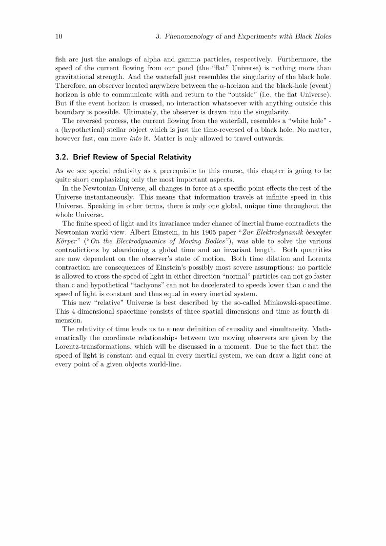
Imagine a pond populated by two kinds of fish — the fast gammas and the slower alphas.The tranquility of the pond is only disturbed by a small creek that flows out of it. Sinceour fish are curious, they send an alpha explorer down the creek. Unfortunately theydo not know that the speed of the water-flow continuously increases down the creek. Soour poor alpha ultimately gets to a point where the water-speed exceeds his maximumswimming capability, a point of no-alpha-return. We call this the α-horizon. From theviewpoint of the fish in the pond something really bad must happen to the alpha at thatpoint; maybe a bigger fish is swallowing it there or a fisherman is catching it. They do notknow for sure what is going on but it definitely must be something “fishy”. But, and thatis the curious thing, for the alpha fish only the water-speed increases a little there. As thepond fish get no sign of life from the brave alpha explorer, they send a fast gamma to lookfor it. The gamma finally reaches the alpha thereby crossing the α-horizon unharmed.The gamma returns to the pond, with considerable effort due to the meanwhile quite

high current and tells the pond-dwellers alpha’s fate. Matter-of-factly these fish are quitehigh on the evolutionary ladder, so their curiousness beats the concerns about risking thelife of another fish. So the heroic gamma again throws itself down the creek. Again, itpasses the α-horizon and again he meets alpha. But now, something has happened: thecurrent has increased so much that even the fastest fish in pond, the gamma-explorer, cannot swim back anymore. We call the point at which the current speed is equal to gamma’sspeed the “black-hole-horizon”. Here again, something “fishy” is noticed by the pond fish,whereas gamma and alpha only feel the slight increase in water-speed. For a picture ofthe pond with all its interesting points, see figure 3.1.So both alpha and gamma are doomed to travel on downwards. Unlucky as they are,

the creek ends in a ripping waterfall! With the help of a great portion luck, both our fishsurvive their ride on the waterfall. They discover that the creek continues to a new pond— obviously getting slower and slower as they get nearer to the new pond.After living there a while, our fish get homesick and try to swim back up the creek.

But, and that is the sad ending of our short story, the countercurrent is too strong for ourgamma at a certain point. So alpha and gamma have to stay in the new pond . . .

Figure 3.1: The pond and the waterfall

Now, back to physics: As the attentive reader might have noticed, alpha and gamma


10 3. Phenomenology of and Experiments with Black Holes

fish are just the analogs of alpha and gamma particles, respectively. Furthermore, thespeed of the current flowing from our pond (the “flat” Universe) is nothing more thangravitational strength. And the waterfall just resembles the singularity of the black hole.Therefore, an observer located anywhere between the α-horizon and the black-hole (event)horizon is able to communicate with and return to the “outside” (i.e. the flat Universe).But if the event horizon is crossed, no interaction whatsoever with anything outside thisboundary is possible. Ultimately, the observer is drawn into the singularity.The reversed process, the current flowing from the waterfall, resembles a “white hole” -

a (hypothetical) stellar object which is just the time-reversed of a black hole. No matter,however fast, can move into it. Matter is only allowed to travel outwards.

3.2. Brief Review of Special RelativityAs we see special relativity as a prerequisite to this course, this chapter is going to bequite short emphasizing only the most important aspects.In the Newtonian Universe, all changes in force at a specific point effects the rest of the

Universe instantaneously. This means that information travels at infinite speed in thisUniverse. Speaking in other terms, there is only one global, unique time throughout thewhole Universe.The finite speed of light and its invariance under chance of inertial frame contradicts the

Newtonian world-view. Albert Einstein, in his 1905 paper “Zur Elektrodynamik bewegterKörper” (“On the Electrodynamics of Moving Bodies”), was able to solve the variouscontradictions by abandoning a global time and an invariant length. Both quantitiesare now dependent on the observer’s state of motion. Both time dilation and Lorentzcontraction are consequences of Einstein’s possibly most severe assumptions: no particleis allowed to cross the speed of light in either direction “normal” particles can not go fasterthan c and hypothetical “tachyons” can not be decelerated to speeds lower than c and thespeed of light is constant and thus equal in every inertial system.This new “relative” Universe is best described by the so-called Minkowski-spacetime.

This 4-dimensional spacetime consists of three spatial dimensions and time as fourth di-mension.The relativity of time leads us to a new definition of causality and simultaneity. Math-

ematically the coordinate relationships between two moving observers are given by theLorentz-transformations, which will be discussed in a moment. Due to the fact that thespeed of light is constant and equal in every inertial system, we can draw a light cone atevery point of a given objects world-line.


3.2. Brief Review of Special Relativity 11

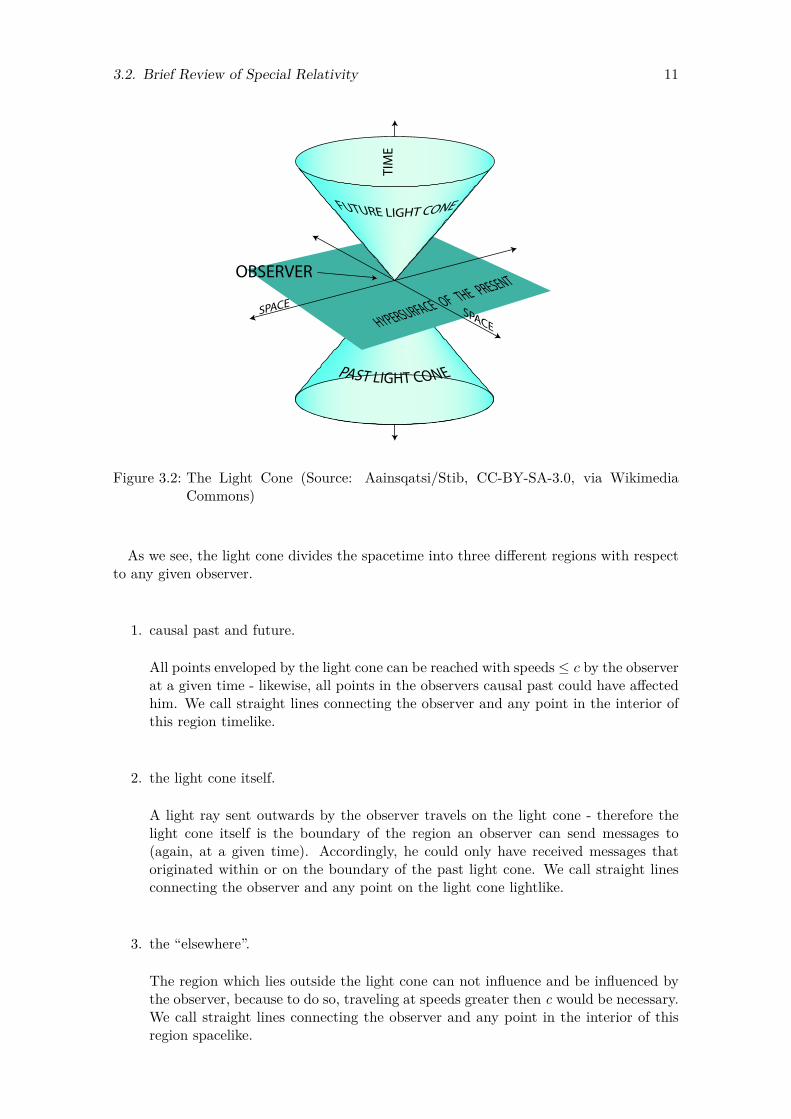
Figure 3.2: The Light Cone (Source: Aainsqatsi/Stib, CC-BY-SA-3.0, via WikimediaCommons)

As we see, the light cone divides the spacetime into three different regions with respectto any given observer.

1. causal past and future.

All points enveloped by the light cone can be reached with speeds ≤ c by the observerat a given time - likewise, all points in the observers causal past could have affectedhim. We call straight lines connecting the observer and any point in the interior ofthis region timelike.

2. the light cone itself.

A light ray sent outwards by the observer travels on the light cone - therefore thelight cone itself is the boundary of the region an observer can send messages to(again, at a given time). Accordingly, he could only have received messages thatoriginated within or on the boundary of the past light cone. We call straight linesconnecting the observer and any point on the light cone lightlike.

3. the “elsewhere”.

The region which lies outside the light cone can not influence and be influenced bythe observer, because to do so, traveling at speeds greater then c would be necessary.We call straight lines connecting the observer and any point in the interior of thisregion spacelike.


https://commons.wikimedia.org/wiki/File:World_line.svg

http://creativecommons.org/licenses/by-sa/3.0/

12 3. Phenomenology of and Experiments with Black Holes

3.3. Mathematical Aspects of Special RelativityTo describe the special causality structure of the Minkowski-spacetime we need a pseudo-Euclidean metric. With µ, ν = t, x, y, z, it reads:

ηµν =

−1 0 0 00 1 0 00 0 1 00 0 0 1

(3.1)

Accordingly,with aµ,bν ∈ R4 we define the inner product:

a · b = aµbνηµν (3.2)

The Minkowski metric is called a pseudo-Euclidean metric because its norm is not positivedefinite.

‖a‖ = aµaνηµν

> 0 : spacelike= 0 : lightlike; with aµ 6= 0< 0 : timelike

(3.3)

In Euclidean space we can change from on set of relative coordinates to another usingarbitrary rotations (here, for simplicity, in a 2-dimensional form):

Λ =(

cosϕ sinϕ− sinϕ cosϕ

)∈ SO(2) (3.4)

ΛT δΛ = δ (3.5)

In 2-dimensional Minkowski spacetime we have to use a hyperbolic rotation matrix to takerespect of the different metric:

Λ =(

cosh ξ sinh ξsinh ξ cosh ξ

)∈ SO(1, 1) (3.6)

With the quantity ξ, sometimes called “rapidity” being defined as

cosh ξ = 1√1− v2

= γ (3.7)

To emphasize the fact that time plays no “special” role (i.e. it is just another coordinate)in special relativity, an exemplary coordinate transformation is shown here:(

t′

x′

)=(

cosh ξ sinh ξsinh ξ cosh ξ

)(tx

)= γ

(t− vxx− vt

)(3.8)


13

4. Metric and Geodesic Equation

In this chapter we will recall metrics in different coordinate systems and we are going toderive the geodesic equation which represents the equation of motion for a point particlein curved spacetime.If we perform an arbitrary change of coordinates in special relativity then the Minkowski

metric ηµν is transformed into a new metric gµν . In order to find this new metric gµν wehave to perform an appropriate sufficiently smooth coordinate transformation by mappingthe old coordinates to the new ones

xi → xi(xk) (4.1)

dxi = ∂xi

∂xkdxk ∂i = ∂xj

∂xi∂j (4.2)

Therefore an infinitesimal line element in the new coordinates can be written as

ds2 = ηijdxidxj = gijdx

idxj = gij∂xi

∂xkdxk

∂xj

∂xldxl (4.3)

Since ds2 has to be invariant due to coordinate transformations we obtain the followingrelation between the components of the new metric components gij and the ones of theold metric components ηij by comparing the coefficients of (4.3)

ηkl = gij∂xi

∂xk∂xj

∂xl(4.4)

4.1. Euclidean Coordinate Transformation

Let us consider a 2-dimensional euclidean metric δij → ds2 = dx2 + dy2 and a coordinatetransformation to polar coordinates r =

√x2 + y2 and ϕ = arctan( yx). Using (4.3) we

obtain for the line element

ds2 = gijdxidxj = grrdr

2 + 2grϕdrdϕ+ gϕϕdϕ2 (4.5)

After evaluating the total derivatives of the new coordinates the line element can be writtenas

ds2 = grr

(xdx+ ydy√x2 + y2

)2

+ 2grϕ

(xdx+ ydy√x2 + y2

)(xdy − ydxx2 + y2

)+ gϕϕ

(xdy − ydxx2 + y2

)2(4.6)

By rearranging the right hand side of (4.6) we get

ds2 = dx2(grr

x2

x2 + y2 − 2grϕxy

(x2 + y2)32

+ gϕϕy2

(x2 + y2)2

)︸︷︷︸

A

+ (4.7a)

dy2(grr

y2

x2 + y2 + 2grϕxy

(x2 + y2)32

+ gϕϕx2

(x2 + y2)2

)︸︷︷︸

B

+ (4.7b)

dxdy

(grr

2xyx2 + y2 + 2grϕ

x2 − y2

(x2 + y2)32− gϕϕ

2xy(x2 + y2)2

)︸︷︷︸

C

(4.7c)


14 4. Metric and Geodesic Equation

Since ds2 is invariant under coordinate transformations it follows that A = B = 1 andC = 0. This yields three linear equations in three variables

A+B = 2 = grr + gϕϕ1r2 (4.8a)

A = 1 =(grrx

2 + gϕϕy2

r2) 1r2 − 2grϕ

xy

(x2 + y2)32

(4.8b)

C = 0 =(grr − gϕϕ

1r2) 2xyx2 + y2 + 2grϕ

x2 − y2

(x2 + y2)32

(4.8c)

⇒ grr = 1 gϕϕ = r2 grϕ = 0 (4.8d)

Hence the line element in polar coordinates is given by

ds2 = gijdxidxj = dr2 + r2dϕ2 (4.9)

4.2. The Geodesic Equation

In order to derive the geodesic equation we will consider two arbitrary points in spacetime.There are two possible ways to find the minimal distance between the two points. Thefirst is the so-called parallel transport where all possible vectors are drawn outwards fromone point, then they are parallel transported until one of these vectors finally “hits” thetarget2. The other method is to find a curve of minimal length connecting the to pointsby variational calculus. We will use this way to derive the geodesic equation, with thelocally shortest connection of two points being called a geodesic.For an arbitrary curve the arc length can be obtained by evaluation of the following integralin the special case of an euclidean metric

τ1∫τ0

dτ

√δijdxi

dτ

dxj

dτ(4.10)

Similarly for a Minkowski metric and spacelike line elements with ds2 > 0 the arc lengthis given by

τ1∫τ0

dτ

√ηijdxi

dτ

dxj

dτ(4.11)

and for timelike line elements with ds2 < 0τ1∫τ0

ds

√−ηij

dxi

dτ

dxj

dτ(4.12)

4.2.1. Geodesics in Euclidean Space

Consider a line element in 2 dimensional euclidean space andy = y(x) : ds2 = dx2

(1 +

(dydx

)2). Hence the arc length of this line element can be

written as

s =x1∫x0

dx

√1 +

(dy

dx

)2(4.13)

2In order to be able to parallel transport a vector one has to find of course a satisfying definition forparallel transported vectors in curved spacetime


4.2. The Geodesic Equation 15

By variation of the arc length (4.13) we can find the path y(x) with minimal arc lengthsuch that δs = 0.

δs =x1∫x0

dx

1√1 +

(dydx

)2

dy

dx

d

dxδy

(4.14)

In order to get rid of the derivative acting on the variation partial integration can be used

δs = 1√1 +

(dydx

)2

dy

dxδy∣∣∣x1

x0︸︷︷︸0

−x1∫x0

dxδy1(

1 +(dydx

)2) 3

2

︸︷︷︸>0

(d2y

dx2

)(4.15)

The boundary term can be dropped by choosing appropriate boundary conditions. Sincethe square root is greater than zero for arbitrary y(x) the variation can only be zero for(

d2y

dx2

)= 0 or dy

dx= ±∞ (4.16)

which is the equation of a straight line in euclidean space in either of the cases. This isindeed the shortest path between two points in euclidean space.

4.2.2. Timelike Geodesics

For an arbitrary metric, a geodesic minimizes the arc length S which for timelike curvesis given by

S =∫ s1

s0ds =

τ1∫τ0

dτ

√−gµν

dxµ

dτ

dxν

dτ(4.17)

The minus sign in front of the metric ensures reality of S for timelike curves. In order toget rid of the square root in S we use a little trick by introducing the einbein. The einbeinis a variable which can be viewed as a parameter “measuring” how fast the curve is beingtraversed as a function of the parameter. Hence the arc length (4.17) can be rewritten as

S = 12

τ1∫τ0

dτ e

(1− e−2gµν

dxµ

dτ

dxν

dτ

)(4.18)

In order to show that this rewritten arc length (4.18) is indeed equal to the original formof the arc length (4.17) the variation in rep-sect of the einbein of the rewritten arc length(4.18) has to vanish

δS

δe= 1

2

τ1∫τ0

dτ

[1 + e−2gµν

dxµ

dτ

dxν

dτ

]= 0 (4.19a)

⇒ e = ±

√−gµν

dxµ

dτ

dxν

dτ(4.19b)

Since the rewritten arc length containing the einbein (4.18) equals the original expressionof the arc length (4.17), the rewritten arc length (4.18) can be varied instead of the original


16 4. Metric and Geodesic Equation

one (4.17) (∂α denotes ∂∂xα ).

δS =12

τ1∫τ0

dτ

[−e−2 (∂αgµν) δxαdx

µ

dτ

dxν

dτ+

d

dτ

e−2gµν δxµ︸︷︷︸δαµδxα

dxν

dτ+ e−2gµν δxν︸︷︷︸

δανδxα

dxµ

dτ

= 0 (4.20)

The variation of the arc length (4.20) has to be zero for arbitrary δα ((xµ) denotes d2xµ

dτ2 ).

e−2gαν xν + e−2gµαx

µ + e−2 (∂βgαν) xβxν + e−2 (∂βgµα) xβxµ−

e−2 (∂αgµν) xµxν + de−2

dτ

(gµνδα

µdxν

dτ+ gµνδα

ν dxµ

dτ

)= 0 (4.21)

The term de−2

dτ (. . . ) can be eliminated by a reparametrization dτ ′ = e dτ which is calledaffine parametrization. Since we want to have an equation of the form xµ + (. . . ) = 0we multiply the reparameterized expression of the variated arc length (4.21) with e2gαγ ,rename some indices (xµ → xν and β → µ) and use gαγgγδ = δα

δ.

2δνγ xν + xµxν (∂µgαν + ∂νgαµ − ∂αgµν) gαγ = 0

⇒ xγ + 12 x

µxν (∂µgαν + ∂νgαµ − ∂αgµν) gαγ = 0 (4.22)

WithΓαµν = 1

2 (∂µgαν + ∂νgαµ − ∂αgµν) (4.23)

being the Christoffel symbols of the first kind. By contracting one index with the metricand multiplying the factor 1

2 we obtain the Christoffel symbols of the second kind Γγµν

Γγµν = gαγΓαµν (4.24)

Hence minimum condition for a geodesic (4.22) can be written as

xγ + Γγµν xµxν = 0 (4.25)

Equation (4.25) is called geodesic equation and determines the equations of motion incurved spacetime, or more general it defines the geodesics in a curved space. To quoteJohn Archibald Wheeler: “Space tells matter how to move and matter tells space how tocurve”. The geodesic equation does indeed relate to the first part of this quote, i.e thatthe movement of a point particle can be determined by the curvature of the spacetime.We will derive the equations that will motivate the second part of this quote in chapter 7.

4.2.3. Geodesics in a Special Metric: The Newton Limit

Consider a metric of the form

ds2 = −(1 + 2φ(xi)

)dt2 + dx2 + dy2 + dz2 xi = (x, y, z) (4.26)

First we have to calculate the Christoffel symbols of the first kind for the metric given forthe line element (4.26)

Γijk = 0 Γtij = 0 Γtti = 12 (∂igtt) = −∂iφ

Γitt = −12 (∂igtt) = ∂iφ Γttt = 0 Γijt = 0


4.2. The Geodesic Equation 17

Since Γγµν = gγαΓαµν the geodesic equation is given by

xγ + gγαΓαµν xµxν =

xt + gttΓtµν xµxν = 0xi + gij︸︷︷︸

δij

Γjttxtxt = 0 (4.27)

With xi = vi, xi = ai and v 1, vµ can be approximated by vµ =(

1 +O(v2)vi

)and the

second equation in (4.27) is simplified to

ai + δij∂jφ = 0~a = −~∇φ ⇒ m~a = −m~∇φ (4.28)

Since we can neglect higher order terms of v we can also neglect the first equation givenby the geodesic equation in (4.27) because it contains such higher order terms of v.For φ one could use −M

r for example. This choice for φ would lead to Newton’s gravitylaw. Hence the interaction between particles with masses can be ascribed to the curvatureof spacetime. Since mass deforms spacetime — a result we are going to derive in chapter7 — the geodesics aren’t straight lines anymore as they would be in flat spacetime andthe equations of motion are given by the geodesic equation. That’s a quite extraordinaryresult, since we only used geometrical principles and were hence able to ascribe gravitationas a geometric phenomenon without the need of a special force. Gravitation can thereforebe “reduced” to a fictitious force. An observer on earth for example seems to be attractedby some kind of gravitational force just because the ground on earth prevents the observerfrom following a geodesic path along the curved spacetime. Without the ground the ob-server would follow his geodesic path and would therefore “feel” no force! Or take forexample an elevator. An observer resting in an elevator which is relatively acceleratingwith respect to a chosen rest frame at 9.81 m

s2 would not be able to tell the difference ofbeing in an relatively accelerating elevator, or being in an relatively resting elevator ina gravitational field. This equivalence of a gravitational field and a corresponding accel-eration of the reference system is a manifestation of the equivalence of gravitational andinertial mass and therefore the mass independence of relative acceleration in a gravitationalfield.

4.2.4. General Geodesics

If the curve whose length we extremize is not timelike, but instead spacelike or lightlike,we have to make minor adjustments to the geodesic action (4.18). The most general caseis covered by extremizing the action

S = k

τ1∫τ0

dτ gµνdxµ

dτ

dxν

dτ(4.29)

with some irrelevant normalization constant k and the additional normalization condition

gµνdxµ

dτ

dxν

dτ=

−1 : timelike

0 : lightlike+1 : spacelike

(4.30)

Note the action (4.29) is essentially equivalent to the action (4.18) provided we choosee = −1. In that case τ is the proper time. In the lightlike or spacelike cases it makesno sense to call τ “proper time”, so in those cases (and in full generality) τ is referred toas “affine parameter”. The action (4.29) is a 1-dimensional analog of the 2-dimensionalPolyakov action of string theory.


18 5. Geodesics for Schwarzschild Black Holes

5. Geodesics for Schwarzschild Black HolesAfter Einstein published the Einstein field equations, Schwarzschild was the first whofound a nontrivial exact solution. We are going to introduce the Schwarzschild solutionand show some important physical results.After the definition of the Schwarzschild metric we look at the asymptotic behavior

of light rays and try to interpret them. The redshift of photons, the perihelion shift ofmercury and the bending of light are important tests of general relativity (especially ofthe Schwarzschild solution) and will be discussed in this chapter. The geodesic equationsare going to tell us something about the trajectories of test particles and the differencesto the Newtonian world.The Schwarzschild solution is not only of great importance in black hole physics, it also

describes the gravitational field in the region outside of ordinary spherically symmetricstars.

5.1. Schwarzschild Solution: Asymptotic Behavior, Light in Radial MotionThe Schwarzschild metric in natural units has the form

ds2 = −(

1− 2Mr

)dt2 + 1

1− 2Mr

dr2 + r2dθ2 + r2 sin2 θdϕ2 (5.1)

The relativistic Schwarzschild solution describes the gravitational field around a sphericalsymmetric mass M which is placed at r = 0.Limits of the Schwarzschild solution:

• r →∞: Asymptotically flat space in spherical coordinates.

• r → 0: True singularity of the spacetime structure.

• r → 2M : The singularity is caused by a breakdown of the coordinates (5.1). Thespacetime is not singular at r = 2M .

• M → 0: Flat space in spherical coordinates.

The only difference of the Schwarzschild solution (5.1) to the Newtonian approximation(4.26) is the dr2 coefficient which asymptotes to the Newtonian result for r → ∞. Thatmeans as long as we are staying far away of the central mass there are only marginaldifferences to Newton’s law of gravity. The closer we get and the heavier the central massbecomes the more our classical approach fails.Let us now derive how light behaves under radial motion. For photons we have to

set ds = 0 and since we are looking at radial motion we also have to set dϕ = dθ = 0.Substituting this into equation (5.1) we obtain the coordinate velocity

dr

dt= ±

(1− 2M

r

)(5.2)

If the light is far away (r → ∞) the coordinate velocity takes the expected value 1.Recalling section 3.1 this is the case where the gamma fish are in the pond and do not feelthe flow of the water. At r = 2M the coordinate velocity is 0. Here the gamma fish wantto swim back but they do not get closer to the pond. So r = 2M is the already mentionedevent horizon of the black hole.Now we want to see what happens to the light ray in its local coordinate system. Here

we have to differentiate the proper time dτ with respect to the proper length dx

dτ2 =(

1− 2Mr

)dt2 dx2 = dr2

1− 2Mr

(5.3)


5.2. Gravitational Redshift (equivalence principle) 19

and using (5.2) we getdx

dτ= dr

dt

11− 2M

r

= ±1 (5.4)

So the light ray has in its local coordinate system the expected velocity 1 (c in SI units).

5.2. Gravitational Redshift (equivalence principle)Consider two static observers OA and OB with the radial coordinates rA and rB in aSchwarzschild geometry. OA sends light signals with the wavelength τA to observer OB.

ds2 = −(

1− 2MrA

)dt2 = − dτA 2 ds2 = −

(1− 2M

rB

)dt2 = − dτB 2 (5.5)

The ratio of the frequency ωA (measured by the emitter) and the frequency ωB (measuredby the observer who receives the signal) results in

ωBωA

= dτAdτB

=

√1− 2M

rA√1− 2M

rB

(5.6)

The closer the emitter comes to rA = 2M the more the frequency ωB gets redshifted (weassume that rA < rB). So for an observer who is looking at an object which is falling intoa black hole it looks like the object moves slower and slower and the frequency gets redderand redder. The observer would never see the emitter reach rA = 2M .We assume that Observer OB is in the asymptotic flat region (rB → ∞) and M

rA 1

(which is the case for an “ordinary body”) we obtainωBωA≈ 1− M

rA(5.7)

∆ωωA

= ωB − ωAωA

≈ −MrA

= φA (5.8)

∆ωωA≈ φA (5.9)

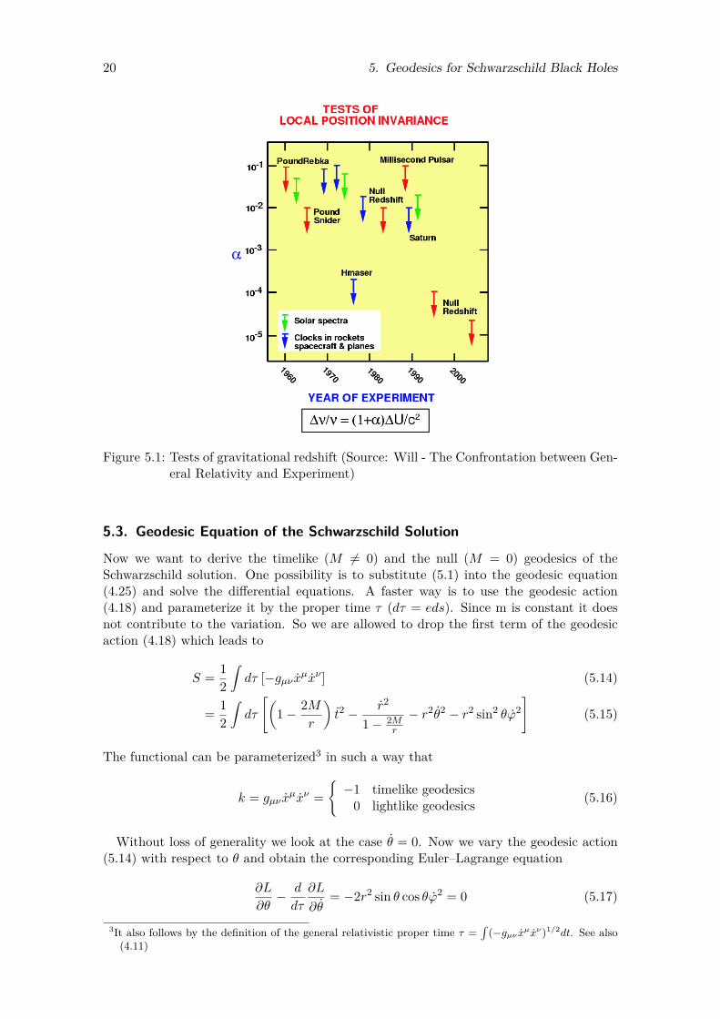
Hence the frequency change equals to the change in potential energy. This effect is knownas gravitational redshift and was observed by Pound and Rebka in 1960 (see figure 5.1).For a stable static spherical body (with dρ/dr ≤ 0 everywhere inside the body) the

theoretical minimal radius rstar for a given mass Mstar is given by

rstar ≥94Mstar . (5.10)

This minimum radius is valid independently of the specific equation of state of the star.We can now use equation (5.6) to estimate what the maximum redshift of light emittedfrom the surface of such a star is

ω∞ωstar

=

√1− 2Mstar

rstar√1− 2M

∞

→ ωstar = 3 (5.11)

The redshift factor is in general given by

z = λB − λAλA

= ωAωB− 1 (5.12)

and leads in our current estimation to an maximal redshift of

zmax = ωstarω∞

− 1 = 2 . (5.13)

This means that observed redshifts of greater than 2 (as measured for example for Quasars)can not arise solely from gravitational redshift of a static spherical body.



Figure 5.1: Tests of gravitational redshift (Source: Will - The Confrontation between Gen-eral Relativity and Experiment)

5.3. Geodesic Equation of the Schwarzschild Solution

Now we want to derive the timelike (M 6= 0) and the null (M = 0) geodesics of theSchwarzschild solution. One possibility is to substitute (5.1) into the geodesic equation(4.25) and solve the differential equations. A faster way is to use the geodesic action(4.18) and parameterize it by the proper time τ (dτ = eds). Since m is constant it doesnot contribute to the variation. So we are allowed to drop the first term of the geodesicaction (4.18) which leads to

S = 12

∫dτ [−gµν xµxν ] (5.14)

= 12

∫dτ

[(1− 2M

r

)t2 − r2

1− 2Mr

− r2θ2 − r2 sin2 θϕ2]

(5.15)

The functional can be parameterized3 in such a way that

k = gµν xµxν =

−1 timelike geodesics

0 lightlike geodesics (5.16)

Without loss of generality we look at the case θ = 0. Now we vary the geodesic action(5.14) with respect to θ and obtain the corresponding Euler–Lagrange equation

∂L

∂θ− d

dτ

∂L

∂θ= −2r2 sin θ cos θϕ2 = 0 (5.17)

3It also follows by the definition of the general relativistic proper time τ =∫

(−gµν xµxν)1/2dt. See also(4.11)


5.3. Geodesic Equation of the Schwarzschild Solution 21

10 20 30 40 50 60

r

-0.05

0.05

0.1

0.15

V

E1

E0

E2

Figure 5.2: The effective potential for the timelike (solid, in the case of L2 > 12M2) andthe Newtonian (dotted) trajectory. L=5,M=1

In general r 6= 0 6= ϕ thus 2 sin θ cos θ = sin (2θ) = 0. Without loss of generality weconsider θ = π

2 . The Euler–Lagrange equations for t and ϕ define two constants of motion

d

dτ

((1− 2M

r

)2t)

= 0 =⇒(

1− 2Mr

)t = F = const (5.18)

d

dτ

(r2ϕ

)= 0 =⇒ r2ϕ = l = const (5.19)

Substituting (5.18) and (5.19) into (5.16) gives

K = F 2

1− 2Mr

− r2

1− 2Mr

− l2

r2 (5.20)

Since the problem is equal to the Kepler problem in the Newtonian case we want to getan equation that looks like

r2

2 + V eff = E (5.21)

5.3.1. Timelike Geodesic

For timelike geodesics (k = −1) we get from (5.20) and (5.21) the effective potential ofthe timelike geodesic

r2

2 −M

r+ l2

2r2 −l2M

r3 = E = F 2 − 12 (5.22)

V eff = −Mr

+ l2

2r2 −l2M

r3 (5.23)

The only difference between the relativistic and the Newtonian trajectory of a massiveparticle is the − l2M

r3 term. The trajectories for different energy levels are (see figure 5.2):



5 10 15 20 25 30

r

0.1

0.2

0.3

0.4

0.5

V

E

Figure 5.3: The effective potential for the lightlike (solid) and the Newtonian (dotted)trajectory. L=5,M=1

E0 At the right side of the maximum of V eff there are stable circular states. If the energyis equal to the minimum of the potential the motion is circular. When that circularstate is slightly perturbed the motion leads to a perihelion shifted elliptic trajectory(see figure 5.4).

E1 Particles left of the maximum will bounce against the potential barrier and fall intothe black hole. Particles on the right side behave similar to the Newtonian case andare able to escape to infinity.

E2 Contrary to the classical physical expectations the particle falls directly towards r = 0.In Kepler’s problem that is only possible for L = 0. If the energy equals to V eff atthe maximum r is zero and the mass point moves on an unstable circular orbit.

5.3.2. Lightlike Geodesic

For lightlike geodesics (k = 0) we get

r2

2 + l2

2r2 −l2M

r3 = E = F 2

2 (5.24)

V eff = l2

2r2 −l2M

r3 (5.25)

The trajectories is similar to the timelike case except that there are no stable circularorbits. Also mind the scale factor of the two figures.

5.4. Orbits of the Schwarzschild Black Hole

The stable circular orbits of the timelike trajectories are the minima of the timelike effectivepotential (5.23)

dV eff

dr= 0 d2V eff

dr2 > 0 (5.26)


5.5. Perihelion shift 23

Figure 5.4: Perihelion shift

The extrema are

r± = l2

2M

1±

√1− 12M2

l2

(r+r− = 3l2

)(5.27)

where r+ is the stable orbit and r− is the unstable orbit (the formula in the parentheseswill be usefull in the next section). Since the square root of the potential should not benegative the bound states are restricted to the condition l2 ≥ 12M2.For the Innermost marginally Stable Circular Orbit we need

d2V eff

dr2 = 0 (5.28)

so the square root of the extrema (5.27) has to vanish

l2 = 12M2 (5.29)⇒ rISCO = 6M (5.30)

We can now, following section 5.2, calculate the maximal redshift for signals from thisorbit

zISCO =(

1− 2M6M

)−1/2− 1 ≈ 0.2 (5.31)

The same can be done for lightlike trajectories to get the Lightlike Unstable CircularOrbit which is always at

rLUCO = 3M (5.32)

5.5. Perihelion shiftFor calculating the perihelion shift in general relativity we assume that the body is at astable circular orbit (meaning that we are in a region near r+) and perturb it slightly. Ifwe would perturb it too much the form of an ellipsis would get lost.The “radius frequency” of the motion is given by

ωr2 = d2V eff

dr2

∣∣∣∣∣r=r+

= 1r+ 4

(3l2 − 2Mr+ − 4Mr−

)(5.33)

(in the last term we have used the equation in the parentheses of (5.27) to eliminate a1/r+ term).With (5.19) we get the angular frequency ωϕ

ωϕ2 = ϕ2 = l2

r4+

(5.34)

and derive (by inserting (5.26) and (5.34) into (5.33))

ωr = ωϕ

(1− 12M2

l2

)1/4

(5.35)

≈ ωϕ

(1− 3M2

l2

)for M l . (5.36)



The precession rate ∆ϕ is the difference between ωr and ωϕ

∆ϕ = T∆ω = 2π (ωϕ − ωr) ≈6πM2

l2(5.37)

If the precession rate is zero the orbit is closed perfectly. This is the case for the Newtoniantheory where we have a effective potential

V eff = −Mr

+ l2

2r2 −l2M

r3 (5.38)

andωr = ωϕ = M2

l3(5.39)

The nonzero ∆ϕ in general relativity leads to a perihelion shift (see figure 5.4).Combining now the Newtonian formula for bound motion

l2

M≈ A(1− e2) (5.40)

with (5.37) leads to

∆ϕ = 6πMA(1− e2) = 6πGM

c2A(1− e2) (5.41)

where e is the eccentricity and A is the aphelion of the ellipsis.This remarkable result can be used to calculate the general relativistic contribution to

the perihelion shift of the Mercury. We have to insert

M ≈ 2 · 1030kg ≈ 1038 (5.42)A ≈ 6· 107km ≈ 4· 1045 (5.43)e ≈ 0.2 (5.44)

into (5.41) to get∆ϕ ≈ 2· 10−5 ≈ 0, 1′′/revolution (5.45)

Since there are around 415 revolutions/century we are now able to compare our calculatedto the observed result

∆ϕ ≈ 42′′/century (5.46)∆ϕobs = (43.11± 0.5)′′/century (5.47)

When Einstein released his work this result was one of the great achievements of generalrelativity.

5.6. Gravitational Light Bending

We are now going to derive another remarkable prediction of general relativity, the grav-itational light-bending. We are searching for a formula for the deflection angle ∆ϕ of alight-ray (which moves on a null geodesic) in the gravitational field of a point source (likethe Sun). So we use the Schwarzschild metric (5.1) and the results we derived for nullgeodesics in the Schwarzschild background in section 5.3.First we establish an integral formula for the azimuthal angle ϕ as a function of the

radial coordinate r. We takeϕ = l

r2 (5.48)


5.6. Gravitational Light Bending 25

∆ϕ

r0

Figure 5.5: Gravitational light bending; ∆ϕ is related to ϕ∞ by ∆ϕ = ϕ∞ − π

and divide it by

r =

√2E − l2

r2 + 2l2Mr3 (5.49)

to getdϕ

dr= 1r2√

2El2 −

1r2 + 2M

r3

(5.50)

To get the total change in of the azimuthal angle ϕ∞ we have to integrate (5.50) between−∞ and +∞ (see figure 5.5). That is the same as integrating twice from the turning pointof the light ray r0 to infinity

ϕ∞ = 2∫ ∞r0

1r2√

2El2 −

1r2 + 2M

r3

dr (5.51)

The integration is more convenient if we make the variable change u = 1/r

ϕ∞ = 2∫ 1/r0

0

1√2El2 − u2 + 2Mu3

du (5.52)

To eliminate E and l we use the fact that

dr

dϕ

∣∣∣∣r0

= 0 (5.53)

which leads to2El2

= 1r0 2 −

2Mr0 3 (5.54)

For the case of flat spacetime we predict a total change of the azimuthal angle ϕ∞ of πwhich leads to a straight line. So we set M = 0 in (5.52) and (5.54) to derive

ϕ∞ = 2∫ 1/r0

0

1√2El2 − u2

du (5.55)

= 2 arctan

u√2El2 − u2

∣∣∣∣∣∣1/r0

0

(5.56)

= π (5.57)

For M 6= 0 the trajectory of the light-ray is no straight line anymore. The deflectionis interpreted as the gravitational attraction of the Schwarzschild geometry. To calculate



the deflection angle ∆ϕ to first order in M we first calculate the change of the angularcoordinate to first order. We substitute (5.54) into (5.52)

ϕ∞ = 2∫ 1/r0

0

du

(r0−2 − 2Mr0−3 − u2 + 2Mu3)1/2 (5.58)

For the total change of the azimuthal angle ϕ∞ in first order ofM we have to differentiateϕ∞ by M and evaluate the result at M = 0

∂(ϕ∞)∂M

∣∣∣∣M=0

= 2∫ 1/r0

0

(r0−3 − u3)du

(r0−2 − 2Mr0−3 − u2 + 2Mu3)3/2

∣∣∣∣∣M=0

(5.59)

= 2∫ 1/r0

0

(r0−3 − u3)

(r0−2 − u2)3/2du (5.60)

= −2√r−2

0 − u2 2 + r0u

1 + r0u

∣∣∣∣1/r0

0(5.61)

= 4r−10 (5.62)

So the deflection angle ∆ϕ in first order of M is

∆ϕ = ϕ∞ − π ≈M∂(ϕ∞)∂M

∣∣∣∣M=0

= 4Mr0

. (5.63)

Inserting

M ≈ 2 · 1030kg ≈ 1038 (5.64)r ≈ 7· 108m ≈ 7 · 1043 (5.65)

predicts a deflection of∆ϕ ≈ 1, 75′′ (5.66)

for light-rays which graze the sun. Eddington proved this gravitational light bending ofstarlight at a solar eclipse in 1919 (up to a measurement accuracy of 10%). Nowadays thethe effect can be measured to an accuracy much better than 1% (see figure 5.6).For more information about the confrontation between General Relativity and experi-

ment see [1].


5.6. Gravitational Light Bending 27

Figure 5.6: Tests for the gravitational light deflection. General relativity predicts γ = 1.The not very precise optical experiments (Optical) were the first conforma-tion of general relativity (the top arrows denote anomalously large values fromearly eclipse expeditions). Later radio-interferometery (Radio) and very-long-baseline radio interferometry (VLBI), produced measurements with greatlyimproved determinations of the deflection of light. (Source: Will - The Con-frontation between General Relativity and Experiment)


28 6. Curvature and Basics of Differential Geometry

6. Curvature and Basics of Differential GeometryGeneral Relativity is a theory of spacetime curvature. Therefore we need to define andintroduce some of the basic concepts of differential geometry and develop the mathematicaltools to thoroughly describe the phenomenons appearing whilst studying black holes.In Chapter 4 we have introduced the concept of a geodesic as shortest lines between

two points in a given spacetime. Additionally, we briefly discussed parallel transport and“autoparallels” (i.e. straightest lines in a spacetime). In Euclidean spacetime, both notionsare identical. In general this is not the case, and we shall see why. It is one of the aimsof this chapter to find circumstances and conditions for arbitrary spacetimes, so that thisequivalence remains true.

6.1. Manifolds and Tangent SpacesWhen visiting an one-year course on topology, you will probably go through sets, enlargethis to topologies and finally arrive at something called a manifold. We do not have timeenough to do so, therefore we will just focus on a special type of manifold - manifolds witha metric - and define them quite sloppily as “something that locally looks like Rn”. Thiscould be a strip of paper, a Moebius strip, our Universe, ...Next to consider is the concept of tangent space. There are various kinds of manifolds.

The ones we are exclusively concerned with have a metric and we can can attach to everypoint x of our manifold a tangent space, a real vector space which intuitively contains thepossible “directions” in which one can tangentially pass through x. For example, if thegiven manifold is a 2-sphere, one can picture the tangent space at a point as the planewhich touches the sphere at that point and is perpendicular to the sphere’s radius throughthe point.

Figure 6.1: Tangent Space of a 2-sphere


6.1. Manifolds and Tangent Spaces 29

By definition, the directional derivatives ∂i in a certain point form a base of the tangentspace attached to this point. This may be illustrated in the following picture:

γ(t)

υ x

TxM

M

Figure 6.2: Tangent vector of a given path on a 2-sphere

This leads us to the next definition: What is a vector? Hopefully, the definition of avector v as linear combination of the base-vectors (v := vµ∂µ) is not new to the reader.More formal, we define a vector as follows:

Assuming we have a manifold M and there exist a smooth maps F : M → R with F ∈ C∞then a tangent vector at point P maps an element of F → R.

v(f) = vµ∂µf f ∈ F (6.1)

A vector must fulfill two criteria (with f, g ∈ F and a, b ∈ R):

1. linearity:v(af + bg) = av(f) + bv(g) (6.2)

2. Leibnitz rule:

v(f · g) = f · v(g) + g · v(f) (6.3)

Linearity combined with the Leibnitz rule implies that a vector acting on any con-stant h vanishes.

⇒ h · v(h) = v(h · h) = 2hv(h) = 0 (6.4)

There are two important facts about tangent spaces. First, the tangent space in pointP (from here on called VP ) fulfills all criteria of a vector space (please, take a look at yourlinear algebra lecture notes for them) and, second, dim(VP ) = dim(M).The next important concept is the dual vector space. To a given vector space VP ,

the dual space V ∗P consists of all linear maps VP → R . About the dimension of V ∗P wemay say:

dim(V ∗P ) = dim(VP ) (6.5)

With e1, · · · , eD being a basis of VP ( ∂∂xn in a coordinate basis) and e1, · · · , eD of V ∗P (dxn

in a coordinate basis), we get:

eµeν = δµν or dxµ(

∂

∂xν

)= δµν (6.6)

This is a generalization of the fact that differentiation (represented by elements of V ∗P ) isthe dual (i.e. inverse) operation of integration—here represented by the elements of VP .Since V ∗∗P = VP vectors can also be seen as linear maps V ∗P → R.



6.2. TensorsA multi-linear map T of the kind

V ∗ ⊗ · · · ⊗ V ∗︸︷︷︸p copies

⊗V ⊗ · · · ⊗ V︸︷︷︸q copies

→ R (6.7)

is called a “tensor of type (p,q)”.Accordingly a

• vector is a (1,0)-tensor,

• dual-vector is a (0,1)-tensor,

• metric is a (0,2) tensor: gµνvµwν = α ∈ R

Taking into account the definition of the basis of vector and dual vector space and definition6.7 we may write an arbitrary (p,q)-tensor in the following form:

T = Tµ1,...,µpν1,...,νqeµ1 ⊗ · · · ⊗ eµp ⊗ eν1 ⊗ · · · ⊗ eνq (6.8)

= Tµ1,...,µpν1,...,νq∂µ1 ⊗ · · · ⊗ ∂µp ⊗ dxν1 ⊗ · · · ⊗ dxνq (6.9)

In this notation, a change of basis can be calculated straightforwardly. With

x′µ = x′µ(xν) (6.10)

∂′µ = ∂

∂x′µ= (∂ν) ∂x

ν

∂x′µ(6.11)

dx′ν = ∂x′ν

∂xµdxµ (6.12)

and the requirement that T is invariant under such transformation (tensors are multi-linearmaps and do not change when altering the basis), we get:

T′α1,...,αq

β1,...,βp= Tµ1,...,µq

ν1,...,νp

∂x′α1

∂xµ1. . .

∂x′αq

∂xµq· ∂x

ν1

∂x′β1. . .

∂xνp

∂x′βp(6.13)

Maybe here is a good point to explain the differences between local and global quantities.When speaking locally, you consider a tensor evaluated at a specific point P . We shallalso call a tensor field loosely “tensor” — the same applies to vectors/vector fields andscalars/scalar fields.


6.3. Another View at the Metric 31

6.3. Another View at the MetricUp until now, we have used the metric only to calculate the length of a vector or the innerproduct between two vectors.With our newly acquired knowledge concerning dual vector-spaces, we are able to interpretthe metric as a map between a given vector space and its dual space.

gµνvν = vµ gµνvν = vµ (6.14)

Even more, this connection provides us with a natural isomorphism of the vector- and thedual-vector space.By multiplying equation 6.14 by gµα from “left”, we obtain

gµαgµνvν = gµαvµ (6.15)

gµνgµαvν = vα (6.16)

⇒ gµνgµα = δαν (6.17)

This last result is important for reasons of consistency.Example: We start with a metric

ds2 = gµνdxµdxν = 2dudr − rdu2 = g′µ′ν′dx

′µ′dx′ν′ (6.18)

where we have xµ = (r, u). We want to make a coordinate transformation to the coordi-nates x′µ′ = (t, R) given by

u = t+ 2 lnR (6.19)

t = R2

4 (6.20)

In general we could just use the the tensor transformation law (6.13) but it is often moreconvenient to use

du = dt+ 2RdR (6.21)

dr = R

2 dR (6.22)

to get

ds2 = −R2

4 dt2 + dR2 (6.23)

or in matrix form

gµν =(−r 11 0

)µν

g′µ′ν′ =(−R2

4 00 1

)µ′ν′

(6.24)



6.4. Covariant DerivativesTo begin with, we have to define the action of a covariant derivative ∇ on an element ofour vector space. With v ∈ V

∇µvα = ∂µvα + Γαµβvβ︸︷︷︸

linear transformation

(6.25)

The last term in equation (6.25) accounts for linear transformations acting on a vectoras it is transported from an element in VP to an element in VP ′ , where P ′ is a pointsufficiently close to P . In other words: the covariant derivative is the derivative along thecoordinates with correction terms which are unspecified at the moment. Now, by lookingat the first term of above equation, we require that the covariant derivative of a vector isa tensor — therefore, we can use what we know about tensor transformation to calculatethe covariant derivative in a new basis. Just inserting into 6.13 yields:

∇′µ′vα′ = ∂xµ

∂xµ′· ∂x

α′

∂xν

(∂µv

ν + Γνµλvλ)

(6.26)

We expand the left-hand side of above equation and rewrite it as transformation of the“old” (unprimed) coordinates:

∂µ′vα′ + Γα′µ′ν′vν

′ = ∂xµ

∂xµ′· ∂x

α′

∂xν∂µv

ν + ∂xµ

∂xµ′· ∂2xα

′

∂xµ∂xνvν + Γα′µ′ν′

∂xν′

∂xνvν

= ∂xµ

∂xµ′· ∂x

α′

∂xν

(∂µv

ν + Γνµλvλ)

(6.27)

This finally leads us to a generic transformation rule of the Γ-element. Note here that wehave not defined this object yet — but the fact that we called it Γ might be a hint that itis equal to the known Christoffel-symbol under certain conditions. . .The transformation rule is:

Γν′µ′λ′ = Γνµλ · ∂xµ

∂xµ′· ∂xλ∂xλ′· ∂xν

′

∂xν −∂xµ

∂xµ′· ∂xλ∂xλ′· ∂2xν

′

∂xµ∂xλ(6.28)

As the Γ-components do not transform as the components of a tensor the quantity Γ it isno tensor. Only the combination of the partial derivative and the Γ-elemtent do transformas a tensor. Generally, the expression Γ is called a “connection”, as it allows to “connect”the tangent spaces at different points that are infinitesimally separated from each other.


6.4. Covariant Derivatives 33

6.4.1. Properties of the Covariant Derivative

In this short subsection we will just list four important properties of the covariant deriva-tive. We do so without proof, but the identities can be checked by inserting definition(6.25). In all definitions T, T are a (p,q)-tensors, α, β ∈ R, v is a vector and f a scalarfunction.

1. Linearity:∇µ

(αT + βT

)= α∇µT + β∇µT (6.29)

2. Leibnitz-Rule:∇µ

(T T

)= (∇µT ) T +

(∇µT

)T (6.30)

3. Consistency with directional derivation:

v(f) = vα∇αf = vα∂αf (6.31)

4. Absence of torsion∇α∇βf = ∇β∇αf (6.32)

5. Metric compatibility (we shall define and use this property below in section 6.7)

Note that 4 and 5 are requirements that are not implicit in the definition (6.25). Let uswrite the equation (6.32) in the following form:

∇a (∂bf) = ∇b (∂af) (6.33)∂a∂bf − Γcab∂cf = ∂b∂af − Γcba∂cf (6.34)

⇒ Γc[a,b] = 0 ⇔ no torsion (6.35)

In equation (6.35) we introduced a new short-hand notation for anti-symmetrization:

Γc[a,b] = 12(Γcab − Γcba

)(6.36)



6.5. Covariant Derivative acting on Dual VectorsUp until now, we have only considered a covariant derivative acting on vectors. To givean overview on covariant derivatives, we have to fill this void. We start with the followingansatz

∇µwν = ∂µwν + Γαµνwα (6.37)

We use now that the covariant derivative of a scalar is equal to its partial derivative (point3. in section 6.4.1) and the Leibnitz-Rule (point 4. in section 6.4.1) to get

∇µ( vαwα︸︷︷︸= scalar

) = ∂µ(vαwα) = vα∂µwα + wα∂µvα (6.38)

= wα(∂µvα + Γαµνvν) + vα(∂µwα + Γβµαwβ) (6.39)

So the combination of the non-underlined terms in above equation has to be zero due andwe conclude that (with a little index renaming)

wαΓαµνvν + vαΓαµνwα = 0 (6.40)

wαvν(Γαµν + Γαµν

)= 0 (6.41)

⇒ Γαµν = −Γαµν (6.42)

Using this result our ansatz now reads:

∇µwν = ∂µwν − Γαµνwα (6.43)

As a consequence we are able to calculate the covariant derivative of a (p,q)-tensor to getan (p,q+1)-tensor:

∇µTµ1,...,µpν1,...,νq = ∂µT

µ1,...,µpν1,...,νq (6.44)

+ Γµ1µαT

αµ2,...,µpν1,...,νq

+ Γµ2µαT

µ1α,...,µpν1,...,νq

+ · · ·++ Γµp µαTµ1,...,α

ν1,...,νq

− Γα ν1µTµ1,...,µp

αν2,...,νq

− · · ·−− Γα νqµT

µ1,...,µpν1,...,α

Despite looking complicated, the rule governing above derivative is quite simple: eachupper index (vector index) leads to a connection term with positive sign, while each lower(dual) index leads to a connection term with negative sign.


6.6. Parallel Transport 35

6.6. Parallel TransportFinally, we arrived at the point where our knowledge on differential geometry is sufficientto discuss parallel transport. Take two vectors v, t ∈ V . Then we call a vector v paralleltransported along t if:

ta∇avb = 0 (6.45)

In the beginning of this chapter we mentioned the auto-parallels. With definition (6.45)

Figure 6.3: Parallel transport on a 2-Sphere (Source: Fred the Oyster, CC BY-SA 4.0, viaWikimedia Commons)

we define an auto-parallel as a curve along a which a vector v is transported parallel toitself.

va∇avb = 0 (6.46)

Expanding this expression results in

va∂avb + Γbacvavc = 0 (6.47)

Since vb = xb; va∂a = ∂τ we arrive at

xb + Γbacxaxc = 0 (6.48)

This is, if Γ = Γ, exactly the geodesic equation (4.25).


https://en.wikipedia.org/wiki/File:Parallel_Transport.svg

https://creativecommons.org/licenses/by-sa/4.0/


6.7. Fixing Γ UniquelyTo derive the Γ we have to impose another condition on parallel transport, namely that iftwo vectors v, w ∈ V are transported parallel along t, the angle between v and w shouldnot change. This means that

ta∇a(gbcv

bwc)

= 0 (6.49)

∀ta, vb, wc. By assumingta∇avb = ta∇awb = 0 (6.50)

we obtaintavbwc (∇agbc) = 0 (6.51)

which is only true ∀ta, vb, wc if∇agbc = 0 (6.52)

Result (6.52) is called “metricity” or “metric compatibility”.As said before, we can use this result and the torsion free condition to derive a unique

Γ. We expand (6.52) and rewrite it twice with permuted indicies:

∇ρgµν = ∂ρgµν − Γλρµgλν − Γλρνgµλ = 0 (6.53)

∇µgνρ = ∂µgνρ − Γλµνgλρ − Γλµρgνλ = 0 (6.54)

∇νgρµ = ∂νgρµ − Γλρνgλµ − Γλµνgλρ = 0 (6.55)

No we subtract (6.53) - (6.54) - (6.55) and with identity (6.35) all underlined and double-underlined terms in the above equations cancel, resulting in the determining equation forΓ:

∂ρgµν − ∂µgνρ − ∂νgρµ + 2Γλµνgλρ = 0 (6.56)

After rearranging this equation, we have finally arrived at the key result:

Γλµν = 12g

λρ (∂µgνρ + ∂νgµρ − ∂ρgµν) = Γλµν (6.57)

In a space-time with no torsion and with metric compatibility, the covariant derivativeis determined by the Christoffel-symbols of the second kind. Thus, the connection isdetermined only by the metric—we call a connection with these properties “Levi-Civita-connection”.


6.8. The Riemann-Tensor 37

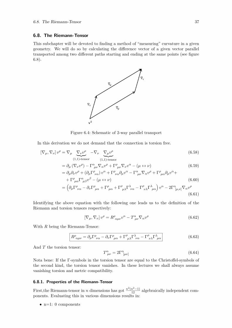
6.8. The Riemann-TensorThis subchapter will be devoted to finding a method of “measuring” curvature in a givengeometry. We will do so by calculating the difference vector of a given vector paralleltransported among two different paths starting and ending at the same points (see figure6.8).

Figure 6.4: Schematic of 2-way parallel transport

In this derivation we do not demand that the connection is torsion free.

[∇µ,∇ν ] vρ = ∇µ ∇νvρ︸︷︷︸(1,1)-tensor

−∇ν ∇µvρ︸︷︷︸(1,1)-tensor

(6.58)

= ∂µ (∇νvρ)− Γαµν∇αvρ + Γρµν∇νvα − (µ↔ ν) (6.59)= ∂µ∂νv

ρ + (∂µΓρνα) vα + Γρνα∂µvα − Γαµν∇αvρ + Γρµα∂µvα++ ΓρµαΓαµβvβ − (µ↔ ν) (6.60)

=(∂µΓρνα − ∂νΓρµα + Γρµα + ΓρµλΓλνα − ΓρνλΓλµα

)vα − 2Γα[µ,ν]∇αv

ρ

(6.61)

Identifying the above equation with the following one leads us to the definition of theRiemann and torsion tensors respectively:

[∇µ,∇ν ] vρ = Rραµνvα − Tαµν∇αvρ (6.62)

With R being the Riemann-Tensor:

Rραµν = ∂µΓρνα − ∂νΓρµα + ΓρµλΓλνα − ΓρνλΓλµα (6.63)

And T the torsion tensor:Tαµν = 2Γα[µν] (6.64)

Nota bene: If the Γ-symbols in the torsion tensor are equal to the Christoffel-symbols ofthe second kind, the torsion tensor vanishes. In these lectures we shall always assumevanishing torsion and metric compatibility.

6.8.1. Properties of the Riemann-Tensor

First,the Riemann-tensor in n dimensions has got n2(n2−1)12 algebraically independent com-

ponents. Evaluating this in various dimensions results in:

• n=1: 0 components



• n=2: 1 component



• n=11: 1210 componentsThe Riemann-tensor has the following symmetries:

Rαβµν = −Rαβνµ (6.65)Rαβµν = −Rβαµν (6.66)Rαβµν = +Rµναβ (6.67)Rα[βµν] = 0 (→ R[αβµν] = 0) (6.68)

There are also some noteworthy contractions of the Riemann-tensor - especially theRicci-tensor and the Ricci-scalar are very important due to their role in Einstein’s generaltheory of relativity.We obtain the (symmetric) Ricci-tensor by contracting the Riemann-tensor over the

“upper” and the third “lower” index:

Rµν := Rρµρν (6.69)

The Ricci-scalar is equal to the trace of the Ricci-tensor:

R := Rµµ (6.70)

When reading literature on differential geometry, you may stumble across the Weyl-tensor(in n ≥ 3 spacetime dimensions):

Cρσµν = Rρσµν −2

n− 2

(gρ[µRν]σ − gσ[µRν]ρ + 2

(n− 2)(n− 1)Rgρ[µgν]σ

)(6.71)

This tensor has sysmmetries equal to those of the Riemann-tensor, but is additionallytraceless with respect to all possible index contractions: Cρµρν = 0.

6.9. Jacobi / Bianchi IdentityLike any other derivative, the covariant derivative satisfies the Jacobi identity:

[[∇λ,∇ρ] ,∇σ] + [[∇ρ,∇σ] ,∇λ] + [[∇σ,∇λ] ,∇ρ] = 0 (6.72)

Which in the context of General Relativity is also known as Bianchi identity. This, whenapplied to the Riemann-curvature-tensor, yields:

∇λRρσµν +∇ρRσλµν +∇σRλρµν = 0 (6.73)

Or, in our short-hand notation∇[λRρσ]µν = 0 (6.74)

One quite interesting result, noteworthy here, is obtained by multiplying (6.73) twicewith the metric:

gνσgµλ · Bianchi identity = ∇µRµρ −∇ρR+∇νRνρ = 0 (6.75)

This leaves us with:∇µ(Rµρ −

12gµρR︸︷︷︸

:= Einstein tensor

)= 0 (6.76)

With the Einstein tensor:Gµρ = Rµρ −

12gµρR (6.77)

In a subsequent chapter - dealing with Einstein’s field equations - the importance of thistensor will become obvious.


6.10. Lie Derivatives 39

6.10. Lie DerivativesThe next important concept to introduce during this differential geometry overview is thatof Lie derivatives - named after Sophus Lie, the Norwegian mathematician who achievedgreat breakthroughs in the field of symmetry transformations. Speaking generally, Liederivatives allow us to evaluate the change of a given vector (or vector field) along thetime evolution of another known vector (or vector field).We start be defining a scalar field Φ (x) = Φ (x). Now we introduce a so-called “diffeomor-phism”, which is an invertible map between two manifolds so that both the function andit’s inverse are smooth. In this case you can visualize it as “moving points on a sphere”

xµ = xµ − ξµ +O(ξ2)

(6.78)

Applying this to the scalar field Φ results in

Φ (x) = Φ (x+ ξ) = Φ (x) = Φ (x) + ξµ∂µΦ (x) +O(ξ2)

(6.79)

In this equation the last term is obtained by Taylor-expansion at x = x. Rewriting thislast statement gives us the definition of the Lie-derivative of Φ (x) in respect to ξ:

LξΦ (x) := Φ (x)− Φ (x) = ξµ∂µΦ (x) (6.80)

Similarly, we define the Lie-derivative of vectors as the Lie-bracket between these twovectors:

Lξvµ := [ξ, v]µ = ξν∂νvµ − vν∂νξµ (6.81)

For dual vectors we use again the Leibniz rule

Lξ(vµwµ

)= wµLξvµ + vµLξwµ = ξα∂α

(vµwµ

)= wµξ

α∂αvµ + vµξα∂αwµ (6.82)

and thus can read off the action of the Lie-derivative on dual vectors:

Lξwµ = ξα∂αwµ + wα∂µξα (6.83)

Again, like with co- and contravariant derivatives, we can use these results to calculatethe Lie-derivative of a (q, p)-tensor:

LξTν1...νq

µ1...µp := ξµ∂µTν1...νq

µ1...µp + Tν1...νq

µµ2...µp ∂µ1ξµ + · · · − T µν2...νq

µ1...µp ∂µξν1 − . . .

(6.84)This expression is equally valid for any symmetric (torsion free) covariant derivative, i.e.,one could substitute everywhere ∂ → ∇ in equation (6.84).



6.11. Killing Vectors

We calculate now the Lie derivative of a metric gµν along a vector ξ.

Lξ (gµν) = ξα∂αgµν + gµα∂νξα + gµα∂µξ

α (6.85)= ξα∇αgµν︸︷︷︸

=0

+gµα∇νξα + gνα∇µξα (6.86)

This simplifies toLξ (gµν) = ∇νξµ +∇µξν (6.87)

A vector that makes the Lie derivate of the metric vanish is called a Killing vector; i.e.a vector ξ is a Killing vector if

Lξ (gµν) = ∇νξµ +∇µξν = 0 (6.88)

Equation (6.88) is called the Killing-equation.Killing vectors generate isometries, meaning that the metric is invariant under the flow

generated by a Killing vector. Thus, every Killing vector generates a certain symmetryand by Noether’s theorem we expect them to produce conserved quantities. We shall seelater how this works in detail when establishing results for the Komar mass and angularmomentum in section 8.4.The existence of Killing vectors can considerably simplify the geometry and often allows

to find exact solutions (even with “paper-and-pencil”), which is another pragmatic reasonwhy Killing vectors are useful.Consider as an example the Schwarzschild metric:

ds2 = −(

1− 2Mr

)dt2 + dr2

1− 2Mr

+ r2dθ2 + r2 sin2 θdϕ2 (6.89)

Here, four Killing vectors exist, namely

ξ0 = ∂t (6.90)ξ1 = ∂φ (6.91)ξ2 = − cosφ∂θ + sinφ cot θ∂φ (6.92)ξ3 = sinφ∂θ + cosφ cot θ∂φ (6.93)

ξ0 creates time translations, so the fact that ξ0 is a Killing vector means that the Schwarzschildmetric (6.89) is static. ξ1...3 generate rotations on a 2-sphere—so, the Schwarzschild metricis spherically symmetric due to the fact that these are Killing vectors. The existence of fourKilling vectors is one way to understand why Schwarzschild was able to find this solutionmerely a few weeks after Einstein wrote down the field equations of general relativity.

6.12. Tensor Densities

An object ist called a tensor density of weight ω if it transforms like

Tα...β = Tα...β∂xα

∂xα. . .

∂xβ

∂xβ

(det

(∂xµ

∂xµ

))ω(6.94)

Hence a tensor density transforms like a tensor under coordinate transformation exceptthat it is additionally weighted by a power of the Jacobian.


6.12. Tensor Densities 41

6.12.1. The Levi-Civita Symbol as a Tensor Density

The Levi-Civita symbol is defined as

εµ1...µD =

+1 for even permutation of µ1 . . . µD

−1 for odd permutation of µ1 . . . µD

0 if 2 or more indices are equal(6.95)

The determinant of a matrix M can also be written with the Levi-Civita-Symbol

εµ1...µD det(M) = εµ1...µDMµ1µ1 . . .M

µDµD (6.96)

Hence the Levi-Civita-Symbol transforms under a general coordinate transformationMµ

µ = ∂xµ

∂xµas

εµ1...µD = det(∂xµ

∂xµ

)εµ1...µD

∂xµ1

∂xµ1. . .

∂xµD

∂xµD(6.97)

This implies that the Levi-Civita-Symbol is a tensor density of weight 1.

In order to get an expression that will allow us to convert tensor densities of weightω into tensors, we recall the transformation of an arbitrary metric.

gµν = ∂xµ

∂xµ∂xν

∂xνgµν (6.98)

Taking the determinant of (6.98) yields

g := det (gµν) (6.99)

g = g

(det

(∂xµ

∂xµ

))−2

(6.100)

The transformation law (6.100) implies that the determinant of a metric is a tensor densityof weight -2. Therefore we can use the determinant of the metric to promote tensordensities of weight ω to tensors.

(tensor density of weight ω) |g|ω2 = tensor (6.101)

Remembering that dDx is a tensor density of weight 1 the result of (6.101) can now beused to create an invariant volume element of the form

dDx |g|12 = invariant volume element (6.102)

dDx can also be written as

dx0 ∧ dx1 ∧ . . . ∧ dxD−1 = 1D! εµ1...µDdx

µ1 ∧ . . . ∧ dxµD (6.103)

Combining the invariant volume element (6.102) and equation (6.103) yields√|g|dx0 ∧ dx1 ∧ . . . ∧ dxD−1 = 1

D!εµ1...µDdxµ1 ∧ . . . ∧ dxµD (6.104)

→ εµ1...µD︸︷︷︸ε-tensor

= εµ1...µD

√|g| (6.105)

This equation for the epsilon tensor (6.105) also shows that the Levi-Civita-Symbol in flatspace(time) equals the epsilon-tensor since in that case

√|g| = 1.



As a useful application let us consider now the covariant action of a free scalar field inD dimensions and derive the Klein–Gordon equation on some arbitrary curved spacetime:

S ∝∫

d Dx√|g|gµν∂µφ∂νφ

→ δS ∝∫

d Dxδφ∂µ(√|g|gµν∂νφ

),

using∂µ

(√|g|gµν∂νφ

)= ∇µ

(√|g|gµν∇νφ

)=√|g|gµν∇µ∇νφ = φ,

this can also be written asδS ∝

∫d Dxδφφ.

The result above can also be used to derive the Laplace equation in arbitrary coordinatesystems.


43

7. Hilbert Action and Einstein Field Equations

In this chapter we derive the Hilbert action. Its variation yields the Einstein equationsthrough the principle of least action. First of all we want to obtain some kind of actionthat depends functionally on the metric.

S[g] =∫

(volume)(scalar) (7.1)

7.1. The Action Integral in QED

We have found an invariant expression for the volume in section 6.12. Only the scalarpart of the action (7.1) has to be determined. In order to achieve this let us first take alittle excursus to quantum electrodynamics. The action in QED should depend on Aµ,the covariant four potential of the electromagnetic field. Using the Minkowski metric thevolume element of the action integral becomes d4x since

√|det (ηµν)| = 1. The only thing

missing is a scalar element in the action integral which depends on Aµ. We can also writethe scalar part of the action integral in terms of a derivative expansion

S [Aµ] =∫d4x [α1AµA

µ + α2∂µAµ + α3 (∂µAν) (∂νAµ) . . .] (7.2)

The action integral should be invariant under gauge transformations Aµ → Aµ = Aµ+∂µχwith χ being an arbitrary scalar field. Therefore the action should only depend on thegauge invariant Faraday tensor Fµν = ∂µAν − ∂νAµ. We hence obtain an expression forthe action integral of the form

S [Aµ] =∫d4x

[αFµνF

µν + βFµνFαβεµναβ+

γ (Fµν)Fµν + δ (FµνFµν)2 + . . .]

(7.3)

This scalar part of the action integral could have an arbitrary number of terms as long asthey are gauge invariant. The dimensions of the coefficients α, β, γ, δ can be obtained bya dimensional analysis. Comparison with the dimension of the volume element which hasthe dimension of a (length)4 and the Faraday tensor which by definition has a dimensionof a (length)−2 yields for α and β no dimension, for γ4 (length)2, for δ (length)4 and forthe higher order term scalars a dimension>(length)4.If a field theory is valid for arbitrary energies/lengths then none of these derivative expan-sion terms could be neglected in the scalar part of the action integral. However, most fieldtheories are not valid for arbitrary energies/lengths. QED for example is only valid upto a certain energy limit which is called UV cut. Since high energies correspond to smalllengths, terms with coefficients that contain higher dimensions of length are suppressedby the UV cut-off scale. Therefore all higher order terms are suppressed by this UV cutoffand only α and β contribute significantly to the action. This leads to an expression of theelectromagnetic action integral like

S [Aµ] =∫d4x

αFµνFµν + βFµνFαβεµναβ︸︷︷︸

boundary term

(7.4)

4dim = −2


44 7. Hilbert Action and Einstein Field Equations

7.2. Hilbert ActionThe derivative expansion used to find an expression for the action in QED can also beused for the scalar part of the Hilbert action integral

S [gµν ] = − 12κ

∫d4x

√|g|[−2Λ +R+ αR2 + βRµνR

µν+

γCµναβCµναβ + . . .

](7.5)

Λ being the cosmological constant, R the Ricci scalar, Rµν the Ricci Tensor and Cµναβthe Weyl tensor. The factor κ = 8π is called gravitational coupling constant and refers tothe strength of the gravitational interaction5. Now let us derive which parts of this actioncan be omitted and which not.If the Lagrangian for the spacetime metric is to be a scalar, it cannot solely depend onthe first derivatives of the metric since ∇αgµν = 0. Since the scalar part of the actionshould contain as few derivations as possible we have to find a scalar consisting of secondderivatives. This leads to the Ricci scalar R as it is the only scalar linear in the secondderivatives of the metric. By analogy to the QED case above we can neglect the higherorder terms proportional to α, β, γ, . . . . Therefore we obtain the Einstein-Hilbert action

S [gµν ] = − 12κ

∫d4x√−g [R− 2Λ] (7.6)

7.3. Einstein Field EquationsThe Einstein field equations can now be obtained by varying the Einstein-Hilbert action(7.6) with respect to the metric (R = gµνRµν).

δS ∝∫dDx

[(δ√−g)

(R− 2Λ) +√−g (δgµνRµν + gµνδRµν)

]= 0 (7.7)

The variation of the first term is pretty straight forward δ√−g = − 1

2√−g δg. First let us

write g as

g = det(M−1gµνM

)=

D∏i=1

λi = exp(

D∑i=1

ln (λi))

= eTr (ln(gµν)), (7.8)

with M being an invertible matrix that brings gµν into upper triangular form and λi theeigenvalues of gµν . This implies

δg = g gµνδgµν = −g gµνδgµν , (7.9)

where we have made use of the relation

δ (gµαgαν) = 0. (7.10)

The variation of the determinant of the metric (7.9) follows directly from the followingrelation

gµνgνα = δµ

α → δ (gµνgνα) = δgµνgνα + gµνδg

να = 0 (7.11)

After this short calculation the variation of the Einstein-Hilbert action is given by

δS =∫dDx√−g

[(Rµν −

12gµνR+ gµνΛ

)δgµν + gµνδRµν

]= 0 (7.12)

5In SI units this factor equals 8πGNc4


7.3. Einstein Field Equations 45

The remaining term gµνδRµν is a boundary term and can hence be dropped.

δRµν =[∂λδΓλµν − ∂µδΓλλν + δΓαµνΓλλα + ΓαµνδΓλλα

− δΓαµλΓλνα − ΓαµλδΓλνα]

(7.13)

This yieldsδRµν = ∇λδΓλµν −∇µδΓλλν︸︷︷︸

boundary term

(7.14)

Therefore we obtain the vacuum Einstein equations

Rµν −12gµνR+ gµνΛ = 0 (7.15)

For many applications Λ is neglected (Λ ≈ 0). Hence the vacuum Einstein equations canoften be simplified to

Rµν −12gµνR = Gµν = 0 (7.16)

and by taking the trace of the vacuum Einstein equaions (7.16)

Tr (Gµν) = R

(1− D

2

)= 0 (7.17)

it follows that the Ricci scalar has to be 0 in higher dimensions i.e D 6= 2. Gµν is calledEinstein tensor. This reduces the Einstein vacuum equations to

Rµν = 0 (7.18)

Even though equation (7.18) looks simple it nevertheless represents 10 non linear coupledPDEs which are very hard to solve6.If we now allow matter to appear in addition to the Einstein-Hilbert action we obtain theinhomogenous Einstein equations

Rµν −12gµνR+ gµνΛ = κTµν (7.19)

The tensor Tµν is called energy-momentum tensor. Taking the covariant divergence of theleft hand side of the inhomogeneous Einstein equations yields zero, since the covariantdivergence of the Einstein tensor vanishes — ∇µGµν = ∇µ

(Rµν − 1

2gµνR

)= 0 — and

due to metric compatibility ∇µ (Λgµν) = 0. Therefore, also the covariant divergence ofthe energy-momentum tensor vanishes.

∇µTµν = 0 (7.20)

Equation (7.20) is called energy-momentum conservation. In chapter 4 we quoted JohnWheeler and found out, that the geodesic equation is equivalent to the statement that“space tells matter how to move”. We also stated, that “matter tells spacetime how tocurve” and promised to derive the equation motivating that statement in this chapter. Ifwe take a closer look at the inhomogeneous Einstein equations (7.19) we see that indeedmatter, or to be more accurate the Energy-Momentum tensor tells spacetime how tocurve. Hence the geodesic equation (4.25) and the inhomogeneous Einstein equations(7.19) motivated the quote of John Wheeler.

6in the case D = 4


46 8. Spherically Symmetric Black Holes and the Birkhoff Theorem

8. Spherically Symmetric Black Holes and the Birkhoff Theorem

In this section we are going to prove that the only spherically symmetric vacuum solu-tion in general relativity is the Schwarzschild solution which is static. Then we discusssome concepts concerning Killing vector fields namely Killing horizons, the Killing vectorlemma and surface gravity. After motivating and introducing global coordinates for theSchwarzschild metric we prove the zeroth law of black hole mechanics. Finally we showhow a mass can be defined in general relativity.

8.1. Birkhoff’s Theorem

We are going to sketch the proof of Birkhoff’s theorem and derive the Schwarzschildsolution

Birkhoff’s theorem: All spherically symmetric vacuum solutions of Einsteins fieldequations are static.

First we have to declare what the terms mean:

• Vacuum solution: Remembering the Einstein equations and looking back to (7.18)vacuum solution means that the Ricci-tensor vanishes Rµν = 0.

• Stationary spacetime: In a stationary spacetime it is possible to find a timelikeKilling vector field7 kµ. This means that if you look at the spacetime after sometime is elapsed it should look the same. More practical insert t 7→ t + a (a is aconstant) into our metric gµν and check if it changes.

As an example imagine a fluid which is rotating around some axis. For the fluid tobe stationary it is allowed to flow as long as the velocity distribution of the fluiddoes not change in time.

• Static spacetime: A spacetime is static if in addition to stationary the Killingvector field is orthogonal to a spacelike hypersurface8. That means if coordinatesare used in which the killing vector kµ = ∂µt the metric is not allowed to have anycross terms of the form dtdxi. Looking for example at the Schwarzschild solution(6.89) we have the Killing vector field kµ = ∂µt ; there are no cross terms dt dxi. Thusthe Schwarzschild spacetime is static.

As another example we use again the example of our rotating fluid. In a staticspacetime the fluid is not allowed to move contrary to the stationary case. It isinteresting to note that the failure of a spacetime to be static is due to not beingtime reflective. While in the case of staticity the time reflection t 7→ −t makes nodifference in stationary spacetimes the cross terms get influenced. The rotating fluidis stationary and not static because the time reflection inverts the rotation direction.

• Spherical symmetric spacetime: With an spherical symmetric spacetime9 wemean a spacetime which has the same symmetries as a 2-sphere i.e. a dΩ2 = dθ2 +sin2 θdϕ2 term.

7This is equivalent to the existence of a one-parameter group of isometries whose orbits are timelikecurves.

8An necessary and sufficient condition for a timelike Killing vector field to be hypersurface orthogonal isk[µ∇νkπ] = 0 (this can be derived using the Frobenius Theorem).

9A more precise definition is: A spherical symmetric spacetime has an isometry group which contains asubgroup isomorphic to the group SO(3). The orbits of the SO(3) have to be 2-spheres.


8.1. Birkhoff’s Theorem 47

Using spherical symmetry one can show10 that the spacetime metric has the form

ds2 = gαβ(xγ)dxαdxβ +X(xγ)dΩ(θ, ϕ)2 (8.1)

where in this case the greek indices only have the values 0, 1. So gαβ(xγ) is a two dimen-sional metric and X(xγ) is a scalar field. We are now able to fix locally our coordinatesxγ in such a way that

X(xγ) = r2 gtr(xγ) = 0 (8.2)

where we use t = x0 and r = x1. So it has the form

ds2 = gtt(t, r)dt2 + grr(t, r)dr2 + r2dΩ2 (8.3)

Since our spacetime is Lorentzian we require gtt(t, r) to be negative and grr(t, r) to bepositive which can be achieved by writing

ds2 = −e2a(t,r)dt2 + e2b(t,r)dr2 + r2dΩ2 (8.4)

Since our metric should be a solution to the vacuum Einstein equations (Rµν = 0) wecalculate now the Ricci tensor. The nonzero components are given by (the dot ˙ means∂/∂t while the prime ′ means ∂/∂r)

Rtt = e2(a−b)(2ra′ + a′2 − a′b′ + a′′

)+ ab− b2 − b = 0 (8.5)

Rtr = 2br

= 0 (8.6)

Rrr = e2(b−a)(b+ b2 − ab

)− a′′ − a′2 + a′b′ + 2

rb′ = 0 (8.7)

Rθθ = e−2b (−1− ra′ + rb′)

+ 1 = 0 (8.8)Rϕϕ = Rθθ sin2 θ = 0 (8.9)

Looking at equation (8.6) we see that Rtr = 0 only if

b(t, r) = 0→ b(t, r) = b(r) (8.10)

which is the first half of Birkhoff’s theorem.Using that (8.9) we calculate

Rθθ = −re−2b(r)a′(t, r) = 0→ a′(t, r) = 0→ a(t, r) = a(r) + f(t) (8.11)

Inserting this into the metric (8.4) gives an −e2(a(r)+f(t))dt2 term. We can parameterizethe time such that dt→ e−f(t)dt. Therefore we have a(t, r) = a(r) and we get the metric

ds2 = −e2a(r)dt2 + e2b(r)dr2 + r2dΩ2 (8.12)

which is stationary since there is no time dependence in the gµν terms. There is atimelike Killing vectorfield kµ = ∂µt where t parametrizes the metric and there are nocross terms with dt which implies staticity and proves Birkhoff’s theorem.Furthermore we are now showing that this solution is the Schwarzschild metric. We

combine (8.5) and (8.7) suitably to get

e2(b−a)Rtt +Rrr = 2r

(a′ + b′) = 0 (8.13)

10See for example [2, Section 5.2] or [3, Appendix B].



which is solved bya(r) = −b(r) + c (8.14)

The constant c can be set to zero since we can again reparametrize dt→ e−cdt.One of the remaining nonzero Ricci tensor components is

Rθθ = 1− e2a(1 + 2ra′) = 1− (re2ar)′ = 0 (8.15)

which leads toe2a = 1 + c

r(8.16)

If we compare the integration constant c with the weak field regime in the Newtonian limit(4.26) we get c = −2M . So our solution is the Schwarzschild solution

ds2 = −(

1− 2Mr

)dt2 + 1

1− 2Mr

dr2 + r2dθ2 + r2 sin2 θdϕ2 (8.17)

So every spherical symmetric vacuum spacetime is described by the Schwarzschild solu-tion. A consequence is that there are no gravitational waves if a spherical symmetric starcollapses.

8.2. Killing vectors

Null hypersurfaces

A general co-dimension 1 hypersurface is defined by some condition on the coordinates,f(xµ) = 0 where f is some smooth function of the coordinates xµ (a simple examplewould be a linear function of the coordinates in 3-dimensional Euclidean space, whichdefines a 2-dimensional plane). The normal vector to this hypersurface is given by k =f(xα)gµν∂νf∂µ, where f 6= 0 is some arbitrary normalization function. If the normalvector becomes null, k2 = 0, the hypersurface is called a null hypersurface.Example: consider constant r hypersurfaces in the Schwarzschild spacetime, f = r−2M .

Then the normal vector has a norm given by k2 = f2gµν(∂µf)(∂νf) = f2grr = (1 −2M/r)f2. The hypersurface becomes a null hypersurface at r = 2M .

Killing horizon

In a stationary spacetime there exists a timelike Killing vector kµ. A null hypersurfaceN is a Killing horizon of a Killing vector field k if, on N , k is normal to N . In the caseof Schwarzschild geometry with the killing vector kµ = (∂t)µ we get the Killing horizonr = 2M

kµkµ = −(

1− 2Mr

)= 0 =⇒ r = 2M (8.18)

Killing vector lemma

Killing vector lemma: ∇µ∇νkρ = Rρνµαkα (8.19)

Before we discuss the consequences of the Killing vector lemma we prove it. RememberKilling’s equation (6.88)

∇(µkν) = 0 (8.20)

We start with the definition of the Riemann tensor

[∇µ,∇ν ] kρ = Rραµνkα (8.21)


8.2. Killing vectors 49

which we expand. With the help of Killing’s equation we get

∇µ∇νkρ +∇ν∇ρkµ = Rραµνkα (8.22)

Now we lower all indices and write down the same equation with permutations of (µνρ)to (νρµ) and (ρµν). If we add the (µνρ) to the (νρµ) term and subtract the (ρµν) termwe obtain

2∇ν∇ρkµ = (Rραµν +Rµανρ −Rναρµ)kα (8.23)

Using the antisymmetry condition Rρ[αµν] = 0 (6.68) leads us to

∇ν∇ρkµ = Rανρµkα (8.24)

Permuting the indices of the Riemann tensor gives

∇ν∇ρkµ = Rµρναkα (8.25)

Renaming and raising the indices completes the proof.As you can see via the Killing vector lemma (8.19) the Killing vector field is completely

determined by kµ and ∇νkµ. So for an n dimensional manifold there are maximally asmany independent Killing vector fields as we are able to construct initial data for kµ and∇νkµ. A maximally symmetric space has

n︸︷︷︸kµ

+ n(n− 1)2︸︷︷︸

∇νkµ is antisymmetric

= n(n+ 1)2 (8.26)

linear independent Killing fields. Consider as an example Euclidean space Rn where wehave n translation and n(n−1)

2 rotation symmetries.

Surface gravity

On a stationary black hole there exists a Killing field kµ which is normal to the horizon.Since kνkν = 0 on the horizon ∇µ(kνkν) is also normal to the horizon. So on the horizonthere exists a function κ defined by

12∇µ(kνkν) = −κkµ (8.27)

κ is the surface gravity of the black hole and is constant on orbits of kµ.To get a explicit formula for κ we use the condition for hypersurface orthogonality of

section 8.1 which leads us tok[µ∇νkρ] = 0 (8.28)

Expanding (8.28) and using Killing’s equation (8.20) we find

kρ∇µkν = −2k[µ∇ν]kρ (8.29)

We multiply it now by the antisymmetric (∇µkν) which makes the brackets on the r.h.s.needless

kρ(∇µkν)(∇µkν) = −2(∇µkν)kµ∇νkρ (8.30)= 2kµ(∇νkµ)∇νkρ (8.31)= ∇ν(kµkµ)∇νkρ (8.32)



Now we use the definition of the surface gravity (8.27) and again Killings’s equation toget

kρ(∇µkν)(∇µkν) = −2κkν∇νkρ (8.33)= 2κkν∇ρkν (8.34)= κ∇ρ(kνkν) (8.35)= −2κ2kρ (8.36)

So the explicit formula for the surface gravity κ evaluated at the horizon H is

κ2 = −12(∇µkν)(∇µkν)

∣∣H (8.37)

Evaluating (8.37) for the Schwarzschild metric gives

κ = 14M (8.38)

Before we come back to Killing vector fields we need to introduce some new concepts.

8.2.1. Spacetime Singularity

We have already mentioned in the beginning of section 5.1 that there are different causesfor singularities. In general it is not easy to determine which type of singularity a regionor point is but we give here some guidelines:

1. Real singularity: The spacetime is in fact singular. One way to prove that a point isa real singularity is by calculating a curvature scalar like RαβχδRαβχδ and show thatit blows up at the suspected region. You have to show that the point can be reachedby an geodesics with some finite affine parameter to show that the singularity is not”at infinity” like e.g. r → ∞ in Schwarzschild. Be aware that it is a sufficient butnot a necessary condition. So even if you are not able to find a curvature scalar thatblows up it could be that there is a real singularity. Conversely if you are able tofind a curvature scalar which blows up at a finite affine parameter you have found areal singularity.

2. Coordinate singularity: The spacetime is nonsingular but the coordinates fail tocover the region properly. In this case we try to find a coordinate transformation ofthe metric where the metric in the new coordinates is not singular anymore. It ispossible to extend the original metric if the transformed metric includes the originalas a proper set.

In Schwarzschild coordinates the calculation of RαβχδRαβχδ shows that there is a realsingularity at r = 0 which can be reached by a geodesic with a finite affine parameter.The singularity at r = 2M will be discussed in the next two sections.

8.2.2. Near horizon region of Schwarzschild geometry

We are now taking a closer look at the near horizon region r = 2M of the Schwarzschildsolution

ds2 = −(

1− 2Mr

)dt2 + 1

1− 2Mr

dr2 + r2dΩ2 (8.39)

We now identify

r − 2M = x2

8M (8.40)



Transforming this equation and substituting the surface gravity for the Schwarzschildmetric (8.38) gives

1− 2Mr

= (κx)2

1 + (κx)2 (8.41)

Near the horizon r = 2M or accordingly at x = 0 we get

1− 2Mr≈ (κx)2 (8.42)

If we differentiate (8.40)dr2 = (κx)2dx2 (8.43)

and insert this and (8.42) into the Schwarzschild solution we get for the near horizon regionr ≈ 2M the Rindler spacetime

ds2 ≈ −(κx)2dt2 + dx2 + 14κ2dΩ2 (8.44)

We now analyze the 2-dim Rindler spacetime

ds2 = −(κx)2dt2 + dx2 x > 0 −∞ < t <∞ (8.45)

This metric seems to be singular at x = 0. Since no curvature invariant shows a badbehavior at x → 0 we guess that it is maybe a coordinate singularity. So we search fora proper coordinate transformation to eliminate the singularity. We first introduce nullcoordinates. They are constant along incoming/outgoing null geodesics. The conditionfor null geodesics parametrized by an affine parameter is

gµνkµkν = −(κx)2t2 + x2 = 0 (8.46)

Transforming (8.46) to (dt

dx

)2= 1

(κx)2 (8.47)

and solving this differential equation for t gives

κt = ± ln x+ constant (8.48)

So we define the outgoing null coordinate u and the ingoing null coordinate v by

u = κt− ln x (8.49)v = κt+ ln x (8.50)

The Rindler metric in our (u, v) coordinates is

ds2 = −ev−udu dv (8.51)

Since our singularity is not removed yet we make another transformation

U = −e−u (8.52)V = ev (8.53)

to getds2 = −dU dV (8.54)

The original Rindler coordinates with x > 0 cover only the U < 0, V > 0 region. Sincethere is no singularity at U = V = 0 anymore we extend our spacetime to−∞ < U, V <∞.



Figure 8.1: Rindler spacetime (Source: Townsend-Black holes: Lecture notes)

Figure 8.2: Worldlines of particles moving at constant x. It is a hyperbolic motion withconstant proper acceleration a = 1

x . (Source: Townsend-Black holes: Lecturenotes)

So in our approximation there are no difficulties at r = 2M . We now make the finaltransformation

T = U + V

2 (8.55)

X = V − U2 (8.56)

to convert the metric in the well known form

ds2 = −dT 2 + dX2 (8.57)

This shows that the Rindler spacetime is the 2-dimensinal Minkowski spacetime in unusualcoordinates.The original Rindler coordinates with x > 0 cover only a certain region (see figure 8.1)

of the Minkowski spacetime (see figure 8.1). The time translation symmetry of the Rindlermetric corresponds to the boost symmetry of Minkowski space (see figure 8.2).The name “surface gravity” can be explained by the following proposition: The surface

gravity κ is the acceleration of a static particle near the horizon as measured at spatialinfinity.So κ is the acceleration a particle needs to stay at a static orbit compared to an observer

at infinity. For more information please take a look at [4, Section 2.3.7]

8.2.3. Global coordinates of the Schwarzschild geometry

In this section we will proceed very similar to the previous section. We start again withthe Schwarzschild metric (8.39) and search for radial null geodesics. They have to satisfy(

dt

dr

)2= 1(

1− 2Mr

)2 (8.58)



Figure 8.3: Collapsing star in ingoing Eddington-Finkelstein coordinates (Source:Townsend-Black holes: Lecture notes)

which can be solved byt = ±r∗ + constant (8.59)

where r∗ denotes the Regge-Wheeler radial coordinate

r∗ = r + 2M ln∣∣∣∣r − 2M

2M

∣∣∣∣ (8.60)

So we define the ingoing radial null coordinate v by

v = t+ r∗ −∞ < v <∞ (8.61)

which leads to the Schwarzschild metric in ingoing Eddington-Finkelstein coordinates(v, r, θ, ϕ)

ds2 = −(

1− 2Mr

)dv2 + 2 dr dv + r2dΩ2 (8.62)

Here we can see already that the metric can be extended to r > 0. To see a collapsing starant the light-cone structure in ingoing Eddington-Finkelstein coordinates look at figure8.3. We define the outgoing radial null coordinate u by

u = t− r∗ −∞ < v <∞ (8.63)

and transform the Schwarzschild metric in outgoing Eddington-Finkelstein coordinates(u, r, θ, ϕ)

ds2 = −(

1− 2Mr

)du2 − 2 dr du+ r2dΩ2 (8.64)

We combine ingoing and outgoing Eddington-Finkelstein coordinates to get

ds2 = −(

1− 2Mr

)du dv + r2dΩ2 (8.65)

We finally introduce

U = −e−u/4M (8.66)V = e−v/4M (8.67)



Figure 8.4: Kruskal diagram of Schwarzschild space. Note that each point corresponds toa 2-sphere. (Source: Townsend-Black holes: Lecture notes)

to get the Schwarzschild metric in Kruskal-Szekeres coordinates

ds2 = −32M3

re−r/2MdU dV + r2dΩ2 (8.68)

where r is given implicitly by

UV = −r − 2M2M er/2M (8.69)

There is no singularity at r = 2M (i.e. U = 0, V = 0) so we are allowed to extend theSchwarzschild solution to all values of U and V which are compatible with r > 0.The Kruskal extension of Schwarzschild spacetime (see figure 8.4) has the following

structure:

• Region I: It is our initial ”outside region“ r > 2M of the Schwarzschild solution.

• Region II: This is the region of the black hole. Once anything crosses the r = 2Mborder between region I and region II it in finite proper time ends up at r = 0 .

• Region III: This time-reversed region of region II is called a white hole. Anythingstaying in this region has to leave region III after finite proper time.

• Region IV: This asymptotically flat space has the same properties as region I. Thereis no possibility of classical communication between region I and region IV.

How serious should we take this diagram? Since the Schwarzschild solution is a vacuumsolution it only describes the region outside of a collapsing star. The past of the spacetimeof a collapsing star is not fully described by the Schwarzschild metric so region III and IVare replaced by the spacetime of the matter distribution (see figure 8.5). Region I and IIhowever, should be taken seriously.


8.3. Zeroth law of black hole mechanics 55

Figure 8.5: Spacetime of a gravitational collapse of a spherical symmetric body. Thedashed region is not described by the Schwarzschild solution (Tµν 6= 0).(Source: Townsend-Black holes: Lecture notes)

Figure 8.6: Orbits of the Killing vector field in Kruskal coordinates. (Source: Townsend-Black holes: Lecture notes)

8.3. Zeroth law of black hole mechanicsWe are now going back to our discussion of Killing vectors. The time translation isometryin Kruskal coordinates is generated by the Killing vector field

kµ = 14M (V ∂V − U∂U )µ (8.70)

which is equal to k = ∂t in region I. It follows that U = 0 and V = 0 are fixed sets (seefigure 8.6). The point U = V = 0 is a fixed point (2-sphere) of kµ called the bifurcationpoint (bifurcation 2-sphere). Note that the Killing field vanishes at this locus. In otherwords, to have a bifurcate Killing horizon we need kµ|S = 0, where S is an (n − 2)-dimensional spacelike hypersurface where the null surfaces generating the Killing horizonintersect.Now we want to prove that the surface gravity κ is constant on the killing horizon. So

we use (8.37) to get

kµ∇µκ2∣∣H = −1

2kµ∇µ

[(∇αkν)(∇αkν)

]∣∣H (8.71)

= −kµ(∇αkν)∇µ∇αkν∣∣H (8.72)



Now use the Killing vector lemma (8.19) and the fact that Rναµρ is antisymmetric (6.65)in (µρ) while the Killing vector fields are symmetric in this indices

kµ∇µκ2∣∣H = −(∇αkν)Rναµρkµkρ

∣∣H = 0 (8.73)

So we have the proof that κ is constant along orbits of kµ.Now we want to prove that κ is also constant on the whole bifurcation 2-sphere S. We

take a vector field tµ tangent to S to prove

tµ∇µκ2∣∣S

= −tµ(∇αkν)∇µ∇αkν∣∣S

= −(∇αkν)Rναµρtµkρ∣∣S

= 0 (8.74)

In the last equality we used that we have a bifurcate Killing horizon, i.e., kρ|S = 0. So κis constant along the bifurcation sphere and we get:Zeroth law of black hole mechanics: κ is constant on a (bifurcate) Killing horizon H.Note that this statement resembles the zeroth law of thermodynamics if we identify

surface gravity κ with temperature (up to some multiplicative constant). Thus, we havea first weak hint that black holes might be thermal states; of course, we need much moreinformation to really conclude this (see the lectures Black Holes II), but the conclusionturns out to be correct.

8.4. Komar massThe Komar mass is a concept of mass in general relativity. Note that is is restricted tostationary spacetimes and it is not the only mass definition in general relativity.In this section we are using Stokes theorem so remember∫

Mdω =

∫∂M

ω (8.75)

∫MdDx

√|g| ∇µV µ =

∫∂M

dD−1x√|γ| nµV µ (8.76)

where γ is the induced metric at the boundary, ∂M is the boundary of M and nµ is theunit normal vector to ∂M .As motivation we discuss the definition of chargeQ in electrodynamics. One of Maxwell’s

equations is∇µF νµ = jν (8.77)

where F νµ is the antisymmetric electromagnetic field tensor and jν is the current density.It is important to note that jν is a conserved quantity

∇ν∇µF νµ = 12[∇ν ,∇µ]F νµ = RνµF

νµ = ∇νjν = 0 (8.78)

Our definition of the ’Komar charge’ is

QK : = 14π

∫Md3x

√|γ| nµjµ (8.79)

= − 14π

∫Md3x

√|γ| nν∇µFµν (8.80)

and leads with the help of Stokes theorem (8.76) to the so called Komar integral

QK = − 14π

∫∂M

d2x√|γ| nνσµFµν (8.81)

where γ is the induced metric at the boundary ∂M and σn is the outward pointing unitnormal. Considering

A0 = QCr

F0r = −∂rA0 = QCr2 (8.82)


8.4. Komar mass 57

shows us that our definition reduces to

QK = − 14π

∫ π

0dθ

∫ 2π

0dφ sin2 θ r2

(−QCr2

)= QC (8.83)

where QC is the Coulomb charge, thus the Komar charge is equivalent to the Coulombcharge.In general relativity the situation is more difficult. We need again a conserved mass-

energy current density∇νjν = 0 (8.84)

If we would define it equivalently to special relativityjν = T νµvµ (8.85)

where vµ is a velocity our conservation condition would require∇νjν = ∇ν(T νµvµ) = (∇νT νµ︸︷︷︸

=0

)vµ + T νµ(∇νvµ)︸︷︷︸=0 if ∇(νvµ)=0

= 0 (8.86)

That means that we need a Killing vector field for a conserved quantity.So we define the conserved current

jµ := Rµνkν (8.87)We suppose now that there is a timelike killing vector kν . We define the Komar mass by

MK : = 14π

∫Md3x

√|γ| nµjµ (8.88)

= 14π

∫Md3x

√|γ| nµRµνkν (8.89)

Inserting the contracted Killing vector lemma (8.19)∇ν∇µkν = Rµνk

ν (8.90)and using Stokes theorem leads to

MK = 14π

∫Md3x

√|γ| nµ∇ν(∇µkν) (8.91)

= 14π

∫∂M

d2x√|γ| nµσν∇µkν (8.92)

With this procedure we are able to construct conserved quantities for different Killingvector fields.We calculate the Komar mass for the Schwarzschild black hole. For unit vectors we have

the requirementsnµn

µ = −1 σµσµ = 1 (8.93)

which lead to

nt =(

1− 2MS

r

) 12

σr =(

1− 2MS

r

)− 12

(8.94)

nµσν∇µkν = ∇tkr = gtt(∂tkr︸︷︷︸=0

+ Γrttkt︸︷︷︸=− 1

2grr∂rgtt

) (8.95)

= −12∂rgtt = MS

r2 (8.96)

Substitute this into our Komar integral (8.92) to get

MK = 14π

∫ π

0dθ

∫ 2π

0dφ sin θ r2MS

r2 = MS (8.97)

Hence our Komar mass definition corresponds to the mass we used in the Schwarzschildmetric.


58 9. Rotating Black Holes: The Kerr Solution

9. Rotating Black Holes: The Kerr SolutionIn this chapter we will discuss rotating black holes. They are described by the Kerr metric.

ds2 = −(∆− a2 sin2 θ

)Σ dt2 − 2a sin2 θ

(r2 + a2 −∆

)Σ dtdϕ+((

r2 + a2)2 −∆a2 sin2 θ)

Σ sin2 θdϕ2 + Σ∆dr2 + Σdθ2 (9.1)

Σ = r2 + a2 cos2 θ ∆ = r2 − 2Mr + a2 a = L

M= const. (9.2)

L denotes the angular momentum and M the mass of the body. Equation (9.1) is calledthe Kerr solution of the Einstein field equations and describes the geometry of spacetimearound a rotating massive body. It is also quite easy to see that if a → 0 i.e. L → 0 inequation (9.1) we recover the Schwarzschild solution which describes non-rotating blackholes. If on the other hand a 6= 0 then we have nontrivial rotation and obtain a spacetimewhich is stationary but not static11.This spacetime has two killing vectors i.e. ∂t and ∂φ. Additionally one can also find an

object called killing tensor kµνwhich also leads to constants of motion like a killing vector,but does not have the same geometrical meaning as a killing vector. This killing tensorsatisfies the killing equation ∇(µkνλ) = 0. We also find two classes of singularities, one for∆ = 0 and one for Σ = 0.The case ∆ = 0 is a coordinate singularity and is the defining equation for the killing

horizons of the killing vectors ξ± = ∂t+Ω±∂φ with Ω± = ar±2+a2 and r± = M±

√M2 − a2.

To see that ∆ = 0 leads to Killing horizons consider the normal vector n ∝ grr∂r whosenorm vanishes when grr = 0, which implies indeed ∆ = 0.The killing horizon for r+ is also the event horizon of the rotating black hole. While

the Kerr metric for r > r+ is able to describe the space outside the outer horizon r+ weknow very little about the region inside the inner horizon r < r− and a solution for theEinstein field equations for this region has still not been discovered yet.The other singularity appears for Σ = 0 which implies r = 0 and θ = π

2 and is calledring singularity because the gravitational singularity for r = 0 is shaped like a ring. Thecurvature invariant RαβγδRαβγδ diverges as we approach Σ = 0.If we compare mass and Kerr parameter of the rotating black hole then we can distin-

guish 3 cases

• M2 > a2 yields 2 killing horizons at r = r± and therefore a Kerr black hole.

• M2 = a2 describes an extremal Kerr black hole where the two killing horizonscoincide and form one event horizon at r = M .

• M2 < a2 would describe a naked singularity that would not be hidden behind anevent horizon i.e. r± would be imaginary.

Since the case M2 < a2 would describe a naked singularity Roger Penrose conceived inthe year 1969 the concept of cosmic censorship conjecture which basically states thatno naked singularities exist in the universe. In 1991 John Preskill and Kip Thorne betagainst Stephen Hawking that the hypothesis was false. Interestingly this was the betHawking lost most clearly even though he was also very close to the up until now acceptedsolution to the problem. In 1997 Hawking conceded the bet because numerical relativistsfound initial data leading to a naked singularity which falsified the strict cosmic censorship11Not static means k[µ∇νkλ] 6= 0 or, equivalently, that the line-element fails to be invariant under time-

inversion t→ −t for a 6= 0.


9.1. Uniqueness Theorem 59

conjecture introduced by Penrose. After this violation of the cosmic censorship conjecturewas discovered, a not less restrictive definition of a cosmic censorship was introduced whichhas not been falsified up until now.Though one may assume that a ratio a

M ≈ 1 would be rare for real black holes, sinceit is an extremal case and that a

M 1 would be the expected common ratio for mostobservable black holes, that is interestingly not the case. For most of the observed blackholes so far a ratio of a

M ≈ 0.1 − 0.98 has been observed. In particular the ratio for theblack hole GRS1915+105 has been observed to be 1 > a

M > 0.98 which is very close tothe extremal black hole limit.

9.1. Uniqueness TheoremThe uniqueness theorem by Carter and Robinson states that if an asymptotically flatspacetime solving the vacuum Einstein field equations which is stationary, axial symmetric,with an event horizon and no singularities outside the horizon, then it has to be the Kerrsolution.This uniqueness theorem makes the Kerr solution one of the most important spacetimes

for black hole physics since nearly every observed black hole up until now is a Kerr blackhole and not a Schwarzschild black hole.

9.2. No-hair TheoremThe no-hair theorem postulates that all black hole solutions of the Einstein-Maxwell equa-tions of gravitation and electromagnetism in general relativity can be completely charac-terized by only three externally observable classical parameters:

• mass

• eletric charge

• angular momentum

All other information about the matter which formed a black hole or is falling into it islost disappears behind the black hole horizon and is therefore permanently inaccessible toexternal observers.

9.3. The ErgosphereAccording to the Kerr solution rotating black holes do not only have more than one Killinghorizon, they also allow an area with very interesting properties to exist called ergosphere.In order to see where this area is located let us consider the time translation killing

vector ka = (∂t)a. With this relation the squared norm is given as

kaka = kbgbak

a = ktgttkt = 0 (9.3)

→ gtt = −(∆− a2 sin2 θ

)Σ = 0 (9.4)

→ r = M +√M2 − a2 cos2 θ (9.5)

The calculated radius (9.5) defines the outer radius of the ergosphere and a sketch of thisergosphere along the killing horizons is given in figure 9.1. The ergosphere is limited bythe radius (9.5) and the event horizon.Note: a particle can enter this ergosphere — unlike the black hole region behind the

event horizon - and leave the region again if it is thrown in the ergosphere region. In orderto remain stationary, however, an observer would have to go faster than light.



Figure 9.1: Kerr black hole horizons and ergosphere

9.4. The Penrose Process

The existence of the ergoregion allows an interesting process where energy can be extractedfrom a rotating black hole, which is called the Penrose process.Assume an unstable particle with Energy E1 > 0 comes from infinity and enters the

ergosphere region. Inside this region the particle decays into two new particles, one withenergy −E2 < 0 and the other one with energy E3 = E1 + E2 > E1. Now one may askwhy a particle with negative energy12 could exist inside this ergoregion. This is possiblebecause the time translation killing vector ka = (∂t)a is spacelike in the ergosphere whichimplies that the energy E = −paka of a particle with four momentum pa can be of eithersign. If the particle with −E2 < 0 now passes the event horizon and the particle withenergy E3 escapes the ergosphere region, the escaped particle would now have more energythan before the decay inside the ergoregion and the black hole must therefore have lostsome of its energy13. Since the surface area of the black hole cannot decrease most of theenergy lost is rotational energy, hence the black hole loses angular momentum during theprocess.Due to this Penrose process one can also find the area theorem mentioned before (see ex.10.2) for black holes which states that the surface area of a black hole cannot decrease.Using this area theorem it is also possible to calculate the amount of radiated energyduring the merger of two axial black holes (see ex. 10.3).

Eout = Ein − Ecap > Ein if Ecap < 0 (9.6)

9.5. Frame-dragging/Thirring-Lense Effect [gravimagnetism]

Frame-dragging means that a rotating spacetime can cause inertial observers to rotateeven if they have no angular momentum. Let us consider such an observer. As weshall see explicitly in section 10.1 the angular momentum parameter is given by ` =gtϕd t/d τ + gϕϕdϕ/d τ so that vanishing ` implies (dϕ/d τ)/(d t/d τ) = −gtϕ/gϕϕ. Theangular coordinate velocity for trajectories with vanishing angular momentum then reads

ω(r, θ) = dϕd t = dϕ

d τ

( d td τ

)−1= − gtϕ

gϕϕ. (9.7)

That fact that ω 6= 0 for ` = 0 is called “frame dragging”.

12The energy that would be measured by an observer at infinity13For more details on this phenomenon called super radiance see e.g. section 4.4.2 in gr-qc/9707012


9.5. Frame-dragging/Thirring-Lense Effect [gravimagnetism] 61

Relatedly, also the Thirring-Lense effect is a phenomenon predicted by general relativityfor non-static (stationary) spacetimes and is caused by rotating bodies which drag space-time around themselves. This effect causes objects to be dragged out of their originalposition relatively to the rotating body. For example an object which moves contrariwise

1Figure 9.2: Frame dragging

on a circular orbit in respect to the rotation of a rotating black hole, would be draggedalong by the black hole spacetime and would be forced to follow the black holes rotation.It is a bit like trying to swim upwards against a current but you are not strong enough toswim upwards so the current drags you along.A satellite orbiting earth for example would not hit the exact point where it started afterone orbit14 and a gyroscope would undergo a precession depending on the location of thegyroscope.One experiment to measure the displacement of satellite orbits15 was done by NASA andthe Italian space agency ASI. The orbits and the displacement of the two satellites LA-GEOS and LAGEOS 2 have been recorded for years and then evaluated, which provedto be very difficult because of the deviation of Earth’s gravitational field from sphericalsymmetry and many other perturbations. In 2004 evaluation of 11 years of position dataled to 99%±5% of the predicted value of orbital displacement. However these results havenot been confirmed by another independent research group evaluating the given data. An-other experiment to measure gravitational effects including frame dragging is the Gravityprobe B experiment. Gravity probe B is a satellite placed in a polar orbit around Earthcontaining four gyroscopes with quartz rotors — the roundest objects ever made —. The

14The predicted effect is small for a body like the earth - about 0,1 mm for an orbit like that of GravityProbe B for example.

15The original task of this experiment involving the two satellites mentioned was a precise determinationof the Earth’s gravitational field.



goal is to measure the precession whose frequency can be determined via

ωµ = −12ε

µνρσξν∇ρξσ, (9.8)

where ξµ is a timelike killing vector16, of these four gyroscopes as accurate as possiblewhich proved to be very difficult. The experiment concluded with an article published inthe journal Physical Rewiev Letters in 2011 which confirmed the precission effect predictedby general relativity caused by frame dragging within an discrepancy of 5%.

x

zaxis of rotation

precession

1

Figure 9.3: Thirring-Lense precession

16For more details see IJMPD 14, Special issue on the Thirring-Lense effect.


63

10. Geodesics for Kerr Black HolesTo derive the geodesics for Kerr black holes we proceed similar to section 5.3. We aregoing to point out the differences of the Kerr geodesics to the Schwarzschild geodesics.Finally we calculate the innermost stable circular orbit.

10.1. Geodesic Equation of the Kerr Black HoleWe assume that θ = π/2. So the Kerr solution (9.1) reduces to

Σ = r2 ∆ = r2 − 2Mr + a2 a = L

M= const. (10.1)

ds2 = −(

1− 2Mr

)dt2 − 4aM

rdtdϕ+ r2

∆dr2 +(r4 + a2 + 2Ma2

r

)dϕ2 (10.2)

We use again the geodesic action (5.14)

S = 12

∫dτ [−gµν xµxν ] (10.3)

= 12

∫dτ

[(1− 2M

r

)t2 + 4aM

rtϕ− r2

∆ r2 −(r2 + a2 + 2Ma2

r

)ϕ2]

(10.4)

Varying the action in order to derive the Euler-Lagrange equations for t and ϕ we findtwo constants of motion (

1− 2Mr

)t+ 2aM

rϕ = F = const (10.5)

− 2aMr

t+(r2 + a2 + 2Ma2

r

)ϕ = l = const (10.6)

In addition we can also write down a corresponding Hamiltonian

F t− lϕ− r2

∆ r2 = k =

1, spacelike Geodesic0, lightlike Geodesic−1, timelike Geodesic.

(10.7)

Solving this two equations for t and ϕ and rearranging the equations to get an equationof the form

r2

2 + V eff = E = F 2 − 12 (10.8)

leads to the effective potential Veff (k = −1)

Veff = −Mr

+ l2 − 2a2E

2r2 −M(l − a

√2E + 1

)2

r3 (10.9)

In comparison to the effective potential of the Schwarzschild case (5.23) we see:• The energy is also in the potential. It is not possible to solve the equation for r andE simultaneous.

• If l2 < 2a2E the centrifugal term gets attractive.

• Both effects are most pronounced for extremal Kerr M2 = a2.For a graphical comparison see figure 10.1.Above we have solved the geodesic equation in the plane θ = π/2. Thanks to the Killing-

tensor of the Kerr solution it turns out that the geodesic equations are integrable evenfor arbitrary values of θ, so that all orbits around the Kerr black hole can be described inclosed form, depending on three constants of motion (in addition to the norm k = −1, 0).


64 10. Geodesics for Kerr Black Holes

1 2 3 4 5 6r2M

-0.4

-0.2

0.2

0.4

VHrL

Extremal Kerr aM=1

Kerr aM=0,99

Kerr aM=12

Schwarzschild

Newton

Figure 10.1: Effective potentials for Newton, Schwarzschild and Kerr

10.2. ISCO of the Kerr Black HoleTo calculate the Innermost (marginally) Stable Circular Orbit of the Kerr solution we usethree algebraic equations in the three unknown r, E and l

V eff = E (10.10)dV eff

dr= 0 (10.11)

d2V eff

dr2 = 0 (10.12)

Since there should be no radial motion r = 0 we get (10.10). Combined with (10.11) itensures circularity of the orbit. To get the innermost marginally stable orbit at r = r∗ wealso need the marginality condition (10.12). We can solve these three algebraic equationsfor r∗, ` and E. Suitably combining them yields a cubic equation for the value of theradius of the ISCO:

r2∗ (r∗ − 6M)2 − 2a2r∗ (3r∗ + 14M) + 9a4 = 0 (10.13)

Solving this equation leads tor∗M

= 3 +√x2 + 3a2/M2 ∓

√(3− x)A (10.14)

A = 3 + x+ 2√x2 + 3a2/M2 (10.15)

x = 1 +(1− a2/M2

)1/3 [(1 + a/M)1/3 + (1− a/M)1/3

], (10.16)

where the upper sign denotes co-rotation and the lower sign represents counter-rotation.If we set a = 0 we see that x = 3 and (10.14) reduces to

r∗ = 6M (10.17)

which is the innermost stable circular orbit rISCO of the Schwarzschild solution.For the extremal Kerr solution (a/M = 1 :→ x = 1, A = 8) the equation leads to

r∗/M = 5∓ 4 (10.18)→ r∗CO = M (10.19)

→ r∗COUNT = 9M (10.20)


10.2. ISCO of the Kerr Black Hole 65

In the case of a counter-rotating test-particle the ISCO of the Kerr Solution is r∗COUNT.For co-rotating particles the ISCO is r∗CO. Since the innermost stable circular orbit r∗COequals to the event horizon of the extremal Kerr Solution there is no gap between theaccretion disc and the horizon. This means that accretion disks in extremal Kerr blackhole backgrounds are able to probe physics close to a black hole horizon. By contrast,in the Schwarzschild black hole there is a gap of minimum 4M between the horizon andsome circular orbit.


66 11. Accretion Discs and Black Hole Observations

11. Accretion Discs and Black Hole ObservationsUp until now we explained and elaborated only theoretical concepts of black hole sciences.This chapter will introduce a method to obtain knowledge about a specific black hole byobserving not the hole itself - which is, matter-of-factedly impossible - but a phenomenonassociated with black holes in binary systems: the accretion disc.In the (quite rare) case that a black hole has formed out of the partner in a binary star

system or a that black hole was “attracted” by a single, massive star, it could be the casethat the black hole starts “sucking” out mass (i.e. matter) from its star-partner. As thismatter streams nearer to the black hole it is heated up (due to inter-particle friction) andultimately starts spiraling into the black hole - and this “spiral” region is what we callaccretion disc. Below is depicted an artists’ impression of such process:

Figure 11.1: Artistic depiction of an accretion disc (Illustration Credit: ESA, NASA, andFelix Mirabel)

So, why are these accretion discs so important to us? As mentioned above, the matteraccredited starts to heat up during the process - thus sending out electromagnetic wavesup to the X-ray spectrum. And these X-rays (more precisely, their spectrum) containsinformation about the spin and mass of the black hole17 and - even more important - theyallow us to distinguish between black holes, neutron stars, protostars and white dwarfs -all of which can form accretion discs in binary systems!This is the point where theory kicks in again - to extract information out of the X-ray

spectrum we need to understand and describe the processes in the accretion discs leadingto the X-ray spectra. From here on we try to establish a (simplified) model of accretiondiscs.

17One model used to describe accretion discs coined by Kip Thorne yields an angular momentum to massratio as |a|

M≤ 0.998.


11.1. Simple Theoretical Model: General Relativistic Perfect Fluid 67

11.1. Simple Theoretical Model: General Relativistic Perfect FluidWe start with an assumption that greatly simplifies our calculation, though it does notcapture all essential aspects of accretion disc physics (in particular, we neglect here vis-cosity and magnetic fields). Our assumption is that we only consider perfect fluids (i.e.with no viscosity). This is owed to the fact the general relativistic fluid dynamics is quitea demanding topic and it would be far beyond the scope of this course to thoroughlyinvestigate it.Furthermore, we define:

• fluid velocity: uµ and its norm: uµuµ = −1

• a density function: ρ

• and the pressure distribution P .

In General Relativity the stress-energy-tensor for perfect fluids reads:

Tµν = (ρ+ P )uµuν + Pgµν (11.1)

This, in flat space with uµuν only having a (0,0)-component, would be Tµν = diag (ρ, P, P, P )For consistency we have to assume conservation of the energy momentum tensor.

∇µTµν = 0 (11.2)

Equation (11.2) imposes a quite strong restriction on the stress-energy-tensor with anastonishing consequence:

∇µTµν = 0 (11.3)uν∇µ ((ρ+ P )uµuν + Pgµν) = 0 (11.4)

uνuµuν︸︷︷︸

=−uµ∇µ (ρ+ P ) + (ρ+ P )

[uν (∇µuν)uµ︸︷︷︸

=−(∇µuµ)

+uν (∇µuν)uµ︸︷︷︸= 1

2∇µ(uνuν)=0

]+ uµg

µν∇µP = 0 (11.5)

− (∇µuµ) (ρ+ P )− uµ∇µ (ρ+ P ) + uµ∇µP = 0 (11.6)

∇µ (uµρ) + P (∇µuµ) = 0 (11.7)

Equation (11.7) is nothing less then the general relativistic continuity equation for idealfluids! In classical mechanics, we need 2 equations to describe ideal fluids - first, the conti-nuity equation (which we’ve already found) and second, a force equation (Euler equation),which we have yet to find.We do so in contracting eq. (11.2) with the projection operator18 δσν + uσuν = Πσ

ν :

(δσν + uσuν)∇µ [(ρ+ P )uµuν ] + (δσν + uσuν)∇νP = 0 (11.8)

(ρ+ P )[∇µ (uµuσ)︸︷︷︸

=uµ∇µuσ+uσ∇µuµ

+uσ uν (∇µuµ)uν︸︷︷︸=−∇µuµ

]+ uµuν (δσν + uσuν)︸︷︷︸

=uµuσ+uµuσ(uµuν)=0

∇µ (ρ+ P ) +

+ (δσν + uσuν)∇νP = 0 (11.9)

(ρ+ P )uµ∇µuσ + (δσν + uσuν)∇νP = 0 (11.10)

These are the force equations for — again — general relativistic, ideal fluids. The onlything left to do now is to prove that — in non-relativistic limits — equations (11.7) and(11.10) are identical to the known continuitiy and Euler equations (11.11) & (11.12):

∂ρ

∂t+ ~∇ · (ρ~v) = 0 (11.11)

18This projection operator satisfies Πµνu

ν = 0 and ΠµνΠν

α = Πµα.


68 11. Accretion Discs and Black Hole Observations

∂ (ρ~v)∂t

+ ~∇ · [~v ⊗ ρ~v] + ~∇P = 0 (11.12)

As done before, we introduce the classic limit by setting

uµ =(1 +O

(v2), vi)

P ρ (11.13)

With this eq. (11.7) reads (N.B.: no curvature):

∇t(ρ ut︸︷︷︸

=1

)+∇i

(ρvi)

+ P(∇tut +∇ivi

)︸︷︷︸

≈0+O(P ·v)

= 0 (11.14)

∂ρ

∂t+ ∂i

(ρvi)≈ 0 +O (P · v) (11.15)

And this is the classic continuity equation. No we apply all limits to eq. (11.10) and resultin:

ρ[∂t~v +

(~v~∇)~v]

+ ~∇P = 0 (11.16)

Taking the difference of (11.16) and (11.12) shows that they are equivalent if the continuityequation holds. Thus we have proved that — in classic limits — both general relativisticfluid equations are identical to the Euler and continuity equations, respectively.Actually, there are some types of perfect fluids — with special equations of state —

these equations apply to:

• dust: P = 0 ⇒ Tµν = ρuµuν

• light-like fluid: ρ = 3P ⇒ Tµµ = 0

• polytropic: P = αρn

• barotropic: P = P (ρ)

Summarizing, the main purpose of this chapter was to learn something about the influenceof the background geometry on a relativistic fluid and the corresponding equation of state.In order to treat real accretion discs one would also have to take into account viscosity

and electromagnetic interactions. This is hard to do in a full general relativistic frameworkand therefore is often done in quasi-Newtonian simulations, where the Newton potentialis replaced by some effective potential similar to (10.9).


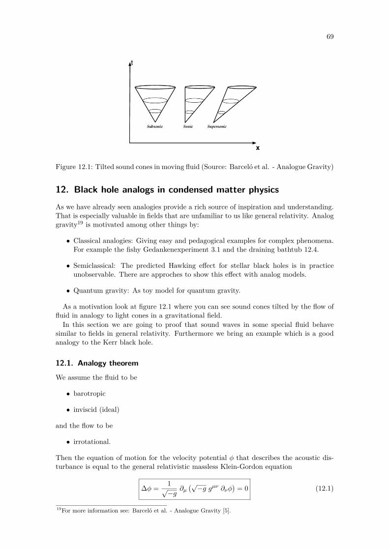
69

Figure 12.1: Tilted sound cones in moving fluid (Source: Barceló et al. - Analogue Gravity)

12. Black hole analogs in condensed matter physics

As we have already seen analogies provide a rich source of inspiration and understanding.That is especially valuable in fields that are unfamiliar to us like general relativity. Analoggravity19 is motivated among other things by:

• Classical analogies: Giving easy and pedagogical examples for complex phenomena.For example the fishy Gedankenexperiment 3.1 and the draining bathtub 12.4.

• Semiclassical: The predicted Hawking effect for stellar black holes is in practiceunobservable. There are approches to show this effect with analog models.

• Quantum gravity: As toy model for quantum gravity.

As a motivation look at figure 12.1 where you can see sound cones tilted by the flow offluid in analogy to light cones in a gravitational field.In this section we are going to proof that sound waves in some special fluid behave

similar to fields in general relativity. Furthermore we bring an example which is a goodanalogy to the Kerr black hole.

12.1. Analogy theorem

We assume the fluid to be

• barotropic

• inviscid (ideal)

and the flow to be

• irrotational.

Then the equation of motion for the velocity potential φ that describes the acoustic dis-turbance is equal to the general relativistic massless Klein-Gordon equation

∆φ = 1√−g

∂µ(√−g gµν ∂νφ

)= 0 (12.1)

19For more information see: Barceló et al. - Analogue Gravity [5].


70 12. Black hole analogs in condensed matter physics

with the acoustic metric

gµν(t, ~x) = ρ

c

[−(c2 − v2) −vi−vj δij

](12.2)

(where i, j = 1..3). The acoustic metric depends on the density ρ, the flow velocity ~v andthe local speed of sound in the fluid c.

12.2. ProofWe start with the continuity equation

∂tρ+ ~∇ · (ρ~v) = 0 (12.3)

and Euler’s equation of inviscid flow

ρ[∂t~v +

(~v · ~∇

)~v]

+ ~∇P = 0 (12.4)

We use the fact that (~v · ~∇

)~v + ~v ×

(~∇× ~v

)= 1

2~∇v2 (12.5)

and get with some manipulations on Euler’s equation

∂t~v = ~v ×(~∇× ~v

)− 1ρ~∇P − 1

2~∇v2 (12.6)

We assume the flow to be irrotational ~∇×~v = 0. Locally the velocity flow is given by thevelocity potential ~v = −~∇φ. Our fluid is also barotropic which means that ρ is a functionof P . That makes it possible to define the specific enthalpy h(P )

h(P ) =∫ p

0

dP ′

ρ(P ′) =⇒ ~∇h = 1ρ~∇P (12.7)

Using the above informations Euler’s equation (12.6) simplifies to

− ∂tφ+ h+ 12(~∇φ)2

= 0 (12.8)

Now we split our equations of motion in background (ρ0, P0, φ0) and linearized fluctu-ations (ερ1, εP1, εφ1)

ρ = ρ0 + ερ1 +O(ε2) (12.9)P = P0 + εP1 +O(ε2) (12.10)φ = φ0 + εφ1 +O(ε2) (12.11)

You can imagine the background as the motion of the fluid “in total”. The linearizedfluctuations are the small relative oscillatory motions known by definition as sound. Asan example you can think of some floating liquid (background) where somewhere in themiddle of this liquid a small disturbance (sound) occurred.We use the Taylor expansions (12.9) and (12.11) to linearize the continuity equation

(12.3) to zeroth

∂tρ0 + ~∇ · (ρ0~v0) = 0 (12.12)

and first order in ε

∂tρ1 + ~∇ · (ρ1~v0 + ρ0~v1) = 0 (12.13)


12.2. Proof 71

Using the barotropic condition we derive

h(P ) = h(P0 + εP1 +O(ε2)) = h(P0) + εh′(P0)P1 +O(ε2) = h0 + εP1ρ0

+O(ε2) (12.14)

With the above result we linearize the Euler equation (12.8) to zeroth

−∂tφ0 + h0 + 12(~∇φ0)2 = 0 (12.15)

and first order in ε

−∂tφ1 + P1ρ0− ~v0 · ~∇φ1 = 0 (12.16)

We transform the last equation to get

P1 = ρ0(∂tφ1 + ~v0 · ~∇φ1) (12.17)

The fact that our fluid is barotropic leads us to

ρ1 = ∂ρ

∂PP1 = ∂ρ

∂Pρ0(∂tφ1 + ~v0 · ~∇φ1) (12.18)

In this equation we recognize the term for the speed of sound

c−2 := ∂ρ

∂P(12.19)

We substitute ρ1 into our linearized continuity equation (12.13) to get the wave equation

∂t

(∂ρ

∂Pρ0(∂tφ1 + ~v0 · ~∇φ1)

)+ ~∇ ·

(∂ρ

∂Pρ0(∂tφ1 + ~v0 · ~∇φ1)~v0 − ρ0~∇φ1

)= 0 (12.20)

Substituting the speed of light in this equation and rearranging the terms leads us to

− ∂t

ρ0c2 (∂tφ1 + ~v0︸︷︷︸

vj0

·~∇φ1)

− ~∇ ·

ρ0c2 [ ~v0︸︷︷︸

vi0

∂tφ1 + ~v0(~v0︸︷︷︸vi0v

j0

·~∇φ1)− c2~∇φ1]

= 0 (12.21)

Since we got rid of the ρ1 and P1 terms we have a wave equation where we just have toknow ρ0 and v0 to solve for φ1. Once we have solved this equation we are able to calculateρ1 and P1 by (12.17) and (12.18). Also observe that if there is no background speed v0 = 0and if the background density is constant the equation (12.21) reduces to the well knownform

∂t2 φ1 = c2∆φ1 (12.22)

We now define the matrix

fµν(t, ~x) := ρ0c2

[−1 −vj0−vi0 (c2δij − vi0v

j0)

](12.23)

and observe that it is possible to write our wave equation (12.21) compactly as

∂µ(fµν∂νφ1) = 0 (12.24)

That looks already similar to our Klein-Gordon equation (g =det(gµν))

∆φ = 1√−g

∂µ(√−g gµν ∂νφ

)= 0 (12.25)



For them to coincide we have to set√−g gµν := fµν (12.26)

We use the determinant property det(aA) = andet(A) for n× n matrices to get

det(fµν) = (√−g)4g−1 = g (12.27)

Expanding the determinant by minors leads to

det(fµν) = − ρ04

c2(12.27)=⇒ g = − ρ0

4

c2 =⇒√−g = ρ0

2

c(12.28)

So we get the inverse acoustic metric

gµν(t, ~x) = 1√−g

fµν = 1ρ0c

[−1 −vj0−vi0 (c2δij − vi0v

j0)

](12.29)

and by matrix inversion the acoustic metric

gµν(t, ~x) = ρ0c

[−(c2 − v2) −vi−vj δij

](12.30)

This completes the proof. Q.e.d

12.3. General remaks• gµν has the signature (−,+,+,+)

• There are two different metrics– Physical spacetime metric: Since we neglect general relativity it is the flat

metric of Minkowski space. It is used for all fluid particles.– Acoustic metric: The sound waves propagate effectively on the acoustic metric.

• Concepts like killing horizon, ergo-region and event horizon generalize to acousticmetrics:– Killing horizon: Equivalent to general relativity (8.18) we calculate kµkµ = 0

with kµ = ∂µt and get |~v| = c for the killing horizon.– Ergo-region: The region where |~v| > c i.e. the region of supersonic flow is an

ergo-region.– Event horizon: Is the boundary of the region from where sound with the speed

of c is not able to escape (see figure 12.2).

12.4. Example: Vortex geometryAs an example we are now considering the vortex geometry which looks similar to adraining bathtub (see figure 12.3). The background velocity potential has the form

φ0 = −A ln(r/a)−B θ (12.31)

which leads to a velocity of the fluid flow of

vi0 = (∂rφ, ∂θφ) = (∂rφ, ∂θφ/r2) = −(A

r,B

r2

)(12.32)


12.4. Example: Vortex geometry 73

Figure 12.2: Trapped surfaces formed by moving fluid. (Source: Barceló et al. - AnalogueGravity)

Figure 12.3: Vortex Geometry: The spirals are the streamlines of the fluid flow. The outercircle is the killing horizon of ∂µt while the inner is the event horizon. Theregion in between is the ergo-region. (Source: Barceló et al. - AnalogueGravity)



and tov2

0 = A2 +B2

r2 (12.33)

Calculating the acoustic metric explicitly leads to

ds2 = −(c2 − A2 +B2

r2

)dt2 − 2A

rdr dt− 2B dθ dt+ dr2 + r2 dθ2 + dz2 (12.34)

The killing horizon is at

rergo =√A2 +B2

c(12.35)

Since for the event horizon only the radial part counts we set B = 0 and get the eventhorizon

rhorizon = |A|c

(12.36)

Given this similarities with the Kerr black hole makes it an interesting and acceptableanalogy.


75

A. Useful formulasThe following formulas were collected by Robert McNess and are available online athttp://jacobi.luc.edu/Useful.html.


http://jacobi.luc.edu/Useful.html

Conventions, Definitions, Identities,and Other Useful Formulae

V

Contents

1 Curvature tensors 1

2 Conventions for Differential Forms 2

3 Euler Densities 3

4 Hypersurfaces 3

5 Sign Conventions for the Action 4

6 Hamiltonian Formulation 5

7 Conformal Transformations 5

8 Small Variations of the Metric 6

9 The ADM Decomposition 8

10 Converting to ADM Variables 10

1. Curvature tensors

Consider a d + 1 dimensional manifold M with metric gµν . The covariant derivative on M that is metric-compatible with gµν is ∇µ.

Christoffel Symbols

Γλµν =1

2gλρ (∂µgρν + ∂νgµρ − ∂ρgµν) (1)

Riemann TensorRλµσν = ∂σΓλµν − ∂νΓλµσ + ΓκµνΓλκσ − ΓκµσΓλκν (2)

Ricci TensorRµν = δσλR

λµσν (3)

Schouten Tensor

Sµν =1

d− 1

(Rµν −

1

2 dgµνR

)(4)

∇νSµν = ∇µSνν (5)

Weyl Tensor

Cλµσν = Rλµσν + gλν Sµσ − gλσ Sµν + gµσ Sλν − gµν Sλσ (6)

1


Commutators of Covariant Derivatives

[∇µ,∇ν ]Aλ = RλσµνAσ (7)

[∇µ,∇ν ]Aλ = RλσµνAσ (8)

Bianchi Identity

∇κRλµσν −∇λRκµσν +∇µRκλσν = 0 (9)

∇νRλµσν = ∇µRλσ −∇λRµσ (10)

∇νRµν =1

2∇µR (11)

Bianchi Identity for Weyl

∇νCλµσν = (d− 2)(∇µSλσ −∇λSµσ

)(12)

∇λ∇σCλµσν =d− 2

d− 1

[∇2Rµν −

1

2dgµν∇2R− d− 1

2d∇µ∇νR−

(d+ 1

d− 1

)R λµ Rνλ (13)

+ CλµσνRλσ +

(d+ 1)

d(d− 1)RRµν +

1

d− 1gµν

(RλσRλσ −

1

dR2

)]

2. Conventions for Differential Forms

p-Form Components

A(p) =1

p!Aµ1...µp dx

µ1 ∧ . . . ∧ dxµp (14)

Exterior Derivative(dA(p)

)µ1...µp+1

= (p+ 1) ∂ [µ1Aµ2...µp+1 ] (15)

B [µ1...µn] :=1

n!

(Bµ1...µn + permutations

)(16)

Hodge-Star

(?A(p)

)µ1...µd+1−p

=1

p!εµ1...µd+1−p

ν1...νp Aν1...νp (17)

? ? =(− 1

)p(d+1−p)+1(18)

Wedge Product

(A(p) ∧B(q)

)µ1...µp+q

=(p+ q)!

p! q!A [µ1...µp Bµp+1...µp+q ] (19)

2


3. Euler Densities

Let M be a manifold with dimension d+ 1 = 2n an even number. Normalized so that χ(S2n) = 2.

Euler Number

χ(M) =

∫

Md 2nx

√g E2n (20)

=

∫

Me2n (21)

Euler Density

E2n =1

(8π)n Γ(n+ 1)εµ1 ...µ2n εν1 ...ν2n R

µ1µ2ν1ν2 . . . Rµ2n−1µ2nν2n−1ν2n (22)

e2n =1

(4π)n Γ(n+ 1)εa1 ...a2nRa1a2 ∧ . . . ∧Ra2n−1a2n (23)

Curvature Two-Form

Rab =

1

2Rab c d ec ∧ ed (24)

Examples

E2 =1

8πεµνελρR

µνλρ (25)

=1

4πR

E4 =1

128π2εµνλρ εαβγδ R

µναβ Rλργδ (26)

=1

32π2

(RµνλρRµνλρ − 4RµνRµν +R2

)

=1

32π2CµνλρCµνλρ −

1

8π2

(d− 2

d− 1

) (RµνRµν −

d+ 1

4 dR2

)

4. Hypersurfaces

Let Σ ⊂M be a d dimensional hypersurface whose embedding is described locally by an outward-pointing, unitnormal vector nµ. Rather than keeping track of the signs associated with nµ being either spacelike or timelike,we will just assume that nµ is spacelike. Indices are lowered and raised using gµν and gµν , and symmetrizationof indices is implied when appropriate.

First Fundamental Form / Induced Metric on Σ

hµν = gµν − nµnν (27)

Projection onto Σ⊥Tµ ... ν ... = hµλ . . . h

σν . . . T

λ ...σ ... (28)

Second Fundamental Form / Extrinsic Curvature of Σ

Kµν = ⊥(∇µnν) = h λµ h σ

ν ∇λnσ =1

2£nhµν (29)

3


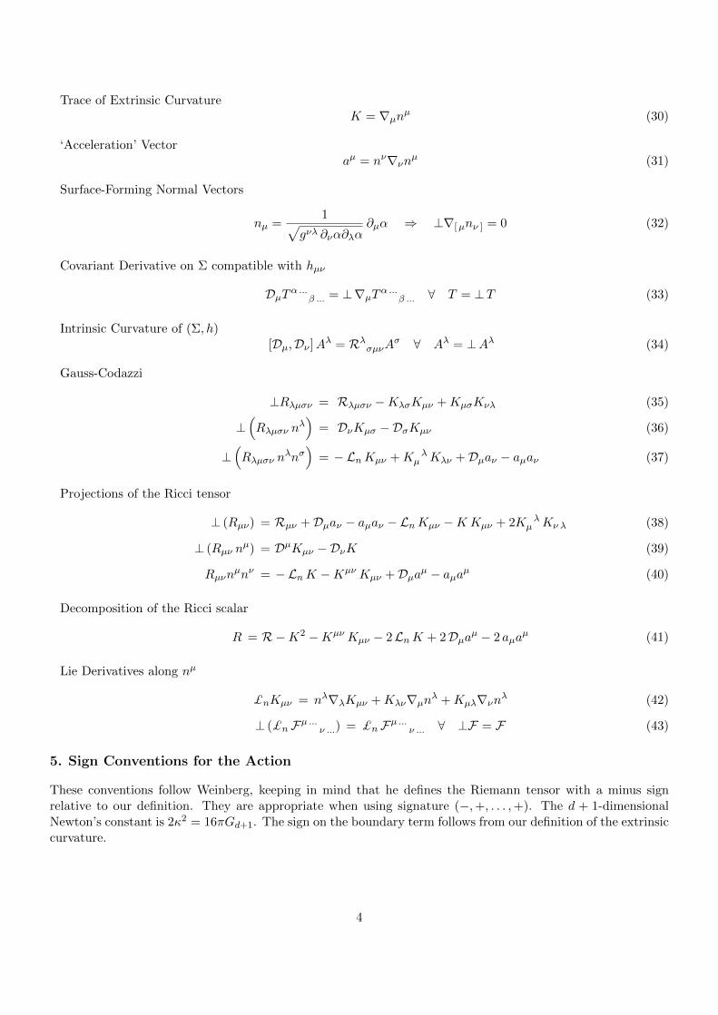
Trace of Extrinsic CurvatureK = ∇µnµ (30)

‘Acceleration’ Vectoraµ = nν∇νnµ (31)

Surface-Forming Normal Vectors

nµ =1√

gνλ ∂να∂λα∂µα ⇒ ⊥∇[µnν ] = 0 (32)

Covariant Derivative on Σ compatible with hµν

DµTα ... β ... = ⊥∇µTα ... β ... ∀ T = ⊥T (33)

Intrinsic Curvature of (Σ, h)[Dµ,Dν ]Aλ = RλσµνAσ ∀ Aλ = ⊥Aλ (34)

Gauss-Codazzi

⊥Rλµσν = Rλµσν −KλσKµν +KµσKνλ (35)

⊥(Rλµσν n

λ)

= DνKµσ −DσKµν (36)

⊥(Rλµσν n

λnσ)

= − LnKµν +K λµ Kλν +Dµaν − aµaν (37)

Projections of the Ricci tensor

⊥ (Rµν) = Rµν +Dµaν − aµaν − LnKµν −KKµν + 2K λµ Kν λ (38)

⊥ (Rµν nµ) = DµKµν −DνK (39)

Rµνnµnν = − LnK −Kµν Kµν +Dµaµ − aµaµ (40)

Decomposition of the Ricci scalar

R = R−K2 −Kµν Kµν − 2LnK + 2Dµaµ − 2 aµaµ (41)

Lie Derivatives along nµ

£nKµν = nλ∇λKµν +Kλν∇µnλ +Kµλ∇νnλ (42)

⊥ (£nFµ ... ν ...) = £nFµ ... ν ... ∀ ⊥F = F (43)

5. Sign Conventions for the Action

These conventions follow Weinberg, keeping in mind that he defines the Riemann tensor with a minus signrelative to our definition. They are appropriate when using signature (−,+, . . . ,+). The d + 1-dimensionalNewton’s constant is 2κ2 = 16πGd+1. The sign on the boundary term follows from our definition of the extrinsiccurvature.

4


Gravitational Action

IG =1

2κ2

∫

Md d+1x

√g(R− 2 Λ

)+

1

κ2

∫

∂Md dx√γ K (44)

=1

2κ2

∫

Md d+1x

√g(R+K2 −Kµν Kµν − 2 Λ

)(45)

Gauge Field Coupled to Particles

IM = − 1

4

∫

Md d+1x

√g FµνFµν (46)

−∑

n

mn

∫dp

(−gµν(xn(p))

dxµn(p)

dp

dxνn(p)

dp

)1/2

(47)

+∑

n

en

∫dpdxµn(p)

dpAµ(xn(p)) (48)

Gravity Minimally Coupled to a Gauge Field

I =

∫

Md d+1x

√g

[1

2κ2(R− 2 Λ)− 1

4FµνFµν

]+

1

κ2

∫

∂Md dx√γ K (49)

6. Hamiltonian Formulation

The canonical variables are the metric hµν on Σ and its conjugate momenta πµν . The momenta are definedwith respect to evolution in the spacelike direction nµ, so this is not the usual notion of the Hamiltonian as thegenerator of time translations.

Bulk Lagrangian Density

LM =1

2κ2

(K2 −Kµν Kµν +R− 2 Λ

)(50)

Momentum Conjugate to hµν

πµν =∂LM

∂ (£nhµν)=

1

2κ2(hµν K −Kµν

)(51)

Momentum Constraint

Hµ =1

κ2⊥ (nνGµν) = 2Dνπµν = 0 (52)

Hamiltonian Constraint

H = − 1

κ2nµnνGµν = 2κ2

(πµν πµν −

1

d− 1π2)

+1

2κ2(R− 2 Λ

)= 0 (53)

7. Conformal Transformations

The dimension of spacetime is d+ 1. Indices are raised and lowered using the metric gµν and its inverse gµν .

Metric

gµν = e 2σ gµν (54)

5


Christoffel

Γλµν = Γλµν + Θλµν (55)

Θλµν = δλµ∇νσ + δλν ∇µσ − gµν ∇λσ (56)

Riemann Tensor

Rλµρν = Rλµρν + δλν ∇µ∇ρσ − δλρ∇µ∇νσ + gµρ∇ν∇λσ − gµν ∇ρ∇λσ (57)

+ δλρ∇µσ∇νσ − δλν ∇µσ∇ρσ + gµν ∇ρσ∇λσ − gµρ∇νσ∇λσ (58)

+(gµρ δ

λν − gµν δλρ

)∇ασ∇ασ (59)

Ricci Tensor

Rµν = Rµν − gµν ∇2σ − (d− 1)∇µ∇νσ + (d− 1)∇µσ∇νσ (60)

− (d− 1) gµν∇λσ∇λσ (61)

Ricci Scalar

R = e−2σ(R− 2 d∇2σ − d (d− 1)∇µσ∇µσ

)(62)

Schouten Tensor

Sµν = Sµν −∇µ∇νσ +∇µσ∇νσ −1

2gµν∇λσ∇λσ (63)

Weyl Tensor

Cλµρν = Cλµρν (64)

Normal Vector

nµ = e−σ nµ nµ = eσ nµ (65)

Extrinsic Curvature

Kµν = eσ(Kµν + hµν n

λ∇λσ)

(66)

K = e−σ(K + dnλ∇λσ

)(67)

8. Small Variations of the Metric

Consider a small perturbation to the metric of the form gµν → gµν + δgµν . All indices are raised and loweredusing the unperturbed metric gµν and its inverse. All quantities are expressed in terms of the perturbation tothe metric with lower indices, and never in terms of the perturbation to the inverse metric. As in the previoussections, ∇µ is the covariant derivative on M compatible with gµν and Dµ is the covariant derivative on ahypersurface Σ compatible with hµν .

Inverse Metricgµν → gµν − gµα gνβ δgαβ + gµα gνβ gλρ δgαλ δgβρ + . . . (68)

6


Square Root of Determinant√g → √g

(1 +

1

2gµνδgµν + . . .

)(69)

Variational Operator

δ(gµν) = δgµν δ 2(gµν) = δ(δgµν) = 0 (70)

δ(gµν) = −gµα gνβ δgαβ δ 2(gµν) = δ(−gµλ gνρ δgλρ

)= 2 gµα gνβ gλρ δgαλ δgβρ (71)

F(g + δg) = F(g) + δF(g) +1

2δ 2F(g) + . . .+

1

n!δ nF(g) + . . . (72)

Christoffel (All Orders)

δ Γλµν =1

2gλρ

(∇µ δgρν +∇ν δgµρ −∇ρ δgµν

)(73)

δ 2 Γλµν = −gλα gρβ δgαβ(∇µ δgρν +∇ν δgµρ −∇ρ δgµν

)(74)

δ n Γλµν =n

2δ n−1

(gλρ) (∇µ δgρν +∇ν δgµρ −∇ρ δgµν

)(75)

Riemann Tensor

δ Rλµσν = ∇σδ Γλµν −∇νδ Γλµσ (76)

Ricci Tensor

δ Rµν = ∇λδ Γλµν −∇νδ Γλµλ (77)

=1

2

(∇λ∇µ δgλν +∇λ∇ν δgµλ − gλρ∇µ∇ν δgλρ −∇2 δgµν

)(78)

Ricci Scalar

δ R = −Rµν δgµν +∇µ(∇ν δgµν − gλρ∇µ δgλρ

)(79)

Surface Forming Normal Vector

δ nµ =1

2nµ n

νnλδgνλ =1

2δgµν n

ν + cµ (80)

cµ =1

2nµ n

νnλδgνλ −1

2δgµν n

ν = −1

2h λµ δgλνn

ν (81)

Extrinsic Curvatures

δ Kµν =1

2nαnβδgαβKµν + δgλρ n

ρ(nµK

λν + nνK

λµ

)(82)

− 1

2hµ

λ hνρnα

(∇λδgαρ +∇ρδgλα −∇αδgλρ

)

δ K = −1

2Kµν δgµν −

1

2nµ(∇νδgµν − gνλ∇µδgνλ

)+Dµcµ (83)

7


9. The ADM Decomposition

The conventions and notation in this section (and the next) are different than what was used in the precedingsections. We consider a d-dimensional spacetime with metric hab.

We start by identifying a scalar field t whose isosurfaces Σt are normal to the timelike unit vector given by

ua = −α∂at , (84)

where the lapse function α is

α :=1√

−hab ∂at ∂bt. (85)

An observer whose worldline is tangent to ua experiences an acceleration given by the vector

ab = uc · d∇cub , (86)

which is orthogonal to ua. The (spatial) metric on the d− 1 dimensional surface Σt is given by

σab = hab + uaub . (87)

The intrinsic Ricci tensor built from this metric is denoted by Rab, and its Ricci scalar is R. The covariantderivative on Σt is defined in terms of the d dimensional covariant derivative as

DaVb := σacσb

e(d∇cVe

)for any Vb = σb

cVc . (88)

The extrinsic curvature of Σt embedded in the ambient d dimensional spacetime (the constant r surfaces fromthe previous section) is

θab := −σacσbd(d∇cud

)= −d∇aub − uaab = −1

2£uσab . (89)

This definition has an additional minus sign, compared to the extrinsic curvature Kµν for the constant r surfacesof the previous section. This is merely for compatibility with the standard conventions in the literature.

Now we consider a ‘time flow’ vector field ta, which satisfies the condition

ta ∂at = 1 . (90)

The vector ta can be decomposed into parts normal and along Σt as

ta = αua + βa , (91)

where α is the lapse function (85) and βa := σabtb is the shift vector. An important result in the derivations

that follow relates the Lie derivative of a scalar or spatial tensor (one that is orthogonal to ua in all of itsindices) along the time flow vector field, to Lie derivatives along ua and βa. Let S be a scalar. Then

£tS = £αuS + £βS = α£uS + £βS . (92)

Rearranging this expression then gives

£uS =1

α

(£tS −£βS

). (93)

Similarly, for a spatial tensor with all lower indices we have

£tWa... = α£uWa... + £βWa... . (94)

8


This is not the case when the tensor has any of its indices raised. In a moment, these identities will allow us toexpress certain Lie derivatives along ua in terms of regular time derivatives and Lie derivatives along the shiftvector βa.

Next, we construct the coordinate system that we will use for the decomposition of the equations of motion.The adapted coordinates (t, xi) are defined by

∂txa := ta . (95)

The xi are d dimensional coordinates along the surface Σt. If we define

Pia :=

∂xa

∂xi, (96)

then it follows from the definition of the coordinates that Pia∂at = 0 and we can use Pi

a to project tensors ontoΣt. For example, in the adapted coordinates the spatial metric, extrinsic curvature, and acceleration and shiftvectors are

σij = PiaPj

bσab (97)

θij = PiaPj

bθab (98)

aj = Pjbab (99)

βi = Piaβa = Pi

ata . (100)

The line element in the adapted coordinates takes a familiar form:

habdxadxb = hab

(∂xa

∂tdt+

∂xa

∂xidxi)(

∂xb

∂tdt+

∂xb

∂xjdxj)

(101)

= hab(tadt+ Pi

adxi)(tbdt+ Pj

bdxj)

(102)

= tatadt2 + 2tadtPi

adxi + habPiaPj

bdxidxj (103)

=(− α2 + βiβi

)dt2 + 2βidtdx

i + σijdxidxj (104)

⇒ habdxadxb = − α2dt2 + σij

(dxi + βidt

)(dxj + βjdt

). (105)

Thus, in the adapted coordinate system we can express the components of the (d dimensional) metric hab andits inverse hab as

hab =

(−α2 + βiβi σijβ

j

σijβj σij

)(106)

hab =

(− 1α2

1α2 β

i

1α2 β

i σij − 1α2 β

iβj

)(107)

det(hab) = −α2 det(σij) (108)

Obtaining the components of the inverse is a short algebraic calculation. Note that the spatial indices ‘i, j, . . .’in the adapted coordinates are lowered and raised using the spatial metric σij and its inverse σij .

In adapted coordinates there are several results concerning the projections of Lie derivatives of scalars andtensors which will be important in what follows. The first, which is trivial, is that the Lie derivative of a scalarS along the time-flow vector ta is just the regular time-derivative

£tS = ta∂aS =∂xa

∂t

∂S

∂xa= ∂tS . (109)

Next, we consider the projector Pia applied to the Lie derivative along ta of a general vector Wa, which gives

Pia£tWa = ∂tWa ∀ Wa . (110)

9


The important point is that this applies not just to spatial vectors but to any vector Wa, as a consequence ofthe result

Pia£tua = 0 . (111)

Finally, we can show that the Lie derivative along ta of any contravariant spatial vector satisfies

P ia£tVa = ∂tV

i ∀ V i = P iaVa . (112)

This follows from a lengthier calculation than what is required for the first two results.Given these results, we can express various geometric quantities and their projections normal to and along

Σt in terms of quantities intrinsic to Σt and simple time derivatives. First, the extrinsic curvature is

θij = − 1

2PiaPj

b£uσab (113)

= − 1

2PiaPj

b

(1

α

(£tσab −£βσab

))(114)

⇒ θij = − 1

2α

(∂tσab −

(Daβb +Dbβa

)). (115)

Since θab is a spatial tensor, projections of its Lie derivative along ua can be expressed in a similar manner

PiaPj

b£uθab =1

α

(∂tθab −£βθab

). (116)

Now we present the Gauss-Codazzi and related equations in adapted coordinates:

PiaPj

b(dRab

)= Rij + θθij − 2θi

kθjk −1

α

(∂tθij −£βθij

)− 1

αDiDjα (117)

Pia(dRabu

b)

= Diθ −Djθij (118)

dRabuaub =

1

α

(∂tθ − βi∂iθ

)− θijθij +

1

αDiD

iα (119)

dR = R+ θ2 + θijθij −2

α

(∂tθ − βi∂iθ

)− 2

αDiD

iα . (120)

10. Converting to ADM Variables

The metric is often presented in the form

habdxadxb = httdt

2 + 2htidtdxi + hijdx

idxj . (121)

We would like to relate these components to the ADM variables: the lapse function α, the shift vector βi, andthe spatial metric σij . This is a fairly straightforward exercise in linear algebra. Comparing with (105), we firstnote that

σij = hij . (122)

The inverse spatial metric, σij , is literally the inverse of hij , which is not the same thing as hij

σij = (σij)−1 = (hij)

−1 6= hij . (123)

For the shift vector we have

hti = σijβj → σikhtk = σikσklβ

l = βi (124)

⇒ βi = σijhtj . (125)

Finally, for the lapse we obtain

α2 = σijhtihtj − htt . (126)

10


86 References

References[1] C. M. Will, “The confrontation between general relativity and experiment,” Living

Reviews in Relativity 9 (2006), no. 3,.

[2] S. M. Carroll, Spacetime and Geometry: An Introduction to General Relativity.Addison Wesley, 2004.

[3] S. Hawking and G. Ellis, The Large scale structure of space-time. CambridgeUniversity Press, 1973.

[4] P. K. Townsend, “Black holes: Lecture notes,” gr-qc/9707012.

[5] C. Barceló, S. Liberati, and M. Visser, “Analogue gravity,” Living Reviews inRelativity 8 (2005), no. 12,.


http://www.arXiv.org/abs/gr-qc/9707012

Documents

BlackHolesIVU - TU Wienquark.itp.tuwien.ac.at/~grumil/pdf/BHLectureNotes.pdf · BlackHolesIVU Lecture notes written by Stefan Prohazka, Max Riegler and Sebastian Singer Supervised