This content has been downloaded from IOPscience. Please scroll down to see the full text.

Download details:

IP Address: 155.33.16.124

This content was downloaded on 11/10/2014 at 12:55

Please note that terms and conditions apply.

Black holes in large N gauge theories

View the table of contents for this issue, or go to the journal homepage for more

2006 Class. Quantum Grav. 23 S927

(http://iopscience.iop.org/0264-9381/23/21/S03)

Home Search Collections Journals About Contact us My IOPscience

INSTITUTE OF PHYSICS PUBLISHING CLASSICAL AND QUANTUM GRAVITY

Class. Quantum Grav. 23 (2006) S927–S956 doi:10.1088/0264-9381/23/21/S03

Black holes in large N gauge theories

Shiraz Minwalla

Tata Institute of Fundamental Research, Mumbai 400 005, India

Received 1 September 2006Published 3 October 2006Online at stacks.iop.org/CQG/23/S927

AbstractGeneralizations of the AdS/CFT correspondence provide a dual Yang–Millsformulation of gravitational physics. In these lectures we investigate the gaugetheoretic description of black holes in AdS5 × S5 and in backgrounds dual toclasses of confining gauge theories. We are motivated by the hope that theYang–Mills description of black holes will shed new light on long-standingpuzzles involving these objects.

PACS number: 04.70.−s

(Some figures in this article are in colour only in the electronic version)

1. Introduction

In 1997 Maldacena argued that certain gravitational systems admit reformulation as gaugetheories. This discovery could prove an important step in our understanding of quantumgravity.

As is well known, the general theory of relativity is incomplete even classically. Generalrelativity evolves generic initial conditions into singular space times. Understanding the‘resolution’ of these singularities (i.e. learning how to evolve space times through them) is oneof the most pressing unsolved problems in the theory of gravity. It seems likely that such aresolution will make crucial use of non-perturbative quantum effects, and has proven difficultto understand directly. The gauge gravity duality could provide a completely new way ofaddressing this issue.

In these lectures we will focus our attention on black holes; singularities that are cloakedbehind event horizons. Event horizon leads to a new set of puzzles. In the mid 1970s Hawkinghad argued that in the presence of black holes, the locality and causality of physics appear tobe in conflict with the unitarity of quantum mechanics. It now seems clear (see below) thatthe formation and evaporation of black holes is, in fact, unitary. Does Hawking’s argumentcontain a subtle flaw? Or are either locality or causality significantly violated in blackhole backgrounds? The gauge gravity duality may prove useful in answering this questionas well.

0264-9381/06/210927+30$30.00 © 2006 IOP Publishing Ltd Printed in the UK S927

S928 S Minwalla

Before we can address these exciting issues, we need a precise description of black holesin gauge theories; the subject of this write-up. In these lectures we will describe the gaugetheoretic description of black holes—to the extent that it has been understood—in two differentsettings; as saddle points in the Euclidean path integral for N = 4 Yang–Mills on S3 and asplasma balls; static lumps of quark gluon plasma in certain confining gauge theories. Ourlectures focus completely on these two examples, and are based almost entirely on [1–4],which may be consulted for more details, as also for a more comprehensive list of referencesto relevant literature. The presentation in these notes closely follows that of my papers [2, 4]written in collaboration with O Aharony, J Marsano, K Papadodimas, M Van Ramsdonk andT Wiseman. Throughout these notes we focus completely on the two examples mentionedabove and do not describe any of the several other interesting attempts that have been made togain gauge theoretic insights into black hole physics.

The constructions we describe in these lectures may or may not eventually prove usefulin resolving singularities, or in solving the Hawking information paradox; that will be decidedby future work.

2. Black holes in AdS5 as saddle points in thermal Yang–Mills on S3

The string dual to N = 4 SYM on S3 × R (where the S3 is taken to be of unit radius) istype IIB string theory on AdS5 × S5, whose metric may be written as

ds2 = R20

(−cosh2 ρ dτ 2 + dρ2 + sinh2 ρ d�23 + d�2

5

). (2.1)

The Hamiltonian of the Yang–Mills theory is identified with the generator of global timetranslations ∂τ in the geometry (2.1). As finite energy excitations in (2.1) are localized aboutρ = 0, it follows immediately from (2.1) that the energy E of the gauge theory on a sphere ofunit radius is related to the proper energy in string theory by Eprop ∼ E/R0. According to thestandard AdS/CFT dictionary, the radius R0 of the AdS5 × S5 space is related to the t’Hooftcoupling λ and the inverse string tension α′ by R0 � λ

14

√α′ (we will ignore all numbers

of order unity in our qualitative discussion). Further, the bulk string coupling g is givenby g = λ

N.

The t’Hooft coupling λ is the loop counting parameter N = 4 U(N) gauge theory; Yang–Mills perturbation theory is reliable only when λ is small. In these lectures we will restrict ourattention throughout to the t’Hooft limit (N → ∞, g2

YM → 0 with λ held fixed). As the bulkstring coupling vanishes in this limit, it follows that N = 4 Yang–Mills on S3 is described byclassical IIB string theory on AdS5 × S5 at every λ. At large λ all length scales in (2.1) arelarge in string units, and the bulk description further simplifies; it reduces to IIB supergravityon the same background.

It turns out that IIB supergravity on AdS5 × S5 hosts a rich spectrum of static black holesolutions. These black holes appear in at least two qualitatively distinct classes. At low energieswe have ‘small’ black holes; solutions that approximate ten-dimensional Schwarzschild blackholes sitting at ρ = 0 in AdS5 space and at any point on the S5. Although these solutionshave never explicitly been constructed, they may be argued to exist at low enough energies.At all energies we also have ‘big black holes’; black holes that are smeared over the S5 (i.e.,whose event horizon has the topology of S3 × S5). These solutions turn out to be dynamicallyunstable at low energies, but become stable at higher energies (of order N2, measured in gaugetheory units) (see [5] and references therein).

In this section we will propose dual descriptions of some of these black holes in EuclideanYang–Mills theory on S3. For this purpose it will be useful first to review the role played bythese black holes in the thermodynamics of IIB theory AdS5 × S5.

Black holes in large N gauge theories S929

2.1. Density of states of weakly coupled IIB theory on AdS5 × S5 at large λ

The density of states of weakly coupled IIB string theory on (2.1) at large R0/√

α′ (large t’Hooftcoupling) is dominated by qualitatively distinct excitations in different energy regimes. See[6] for a more detailed discussion than the one we will present here.

Gravitons. The only states in the spectrum with proper energy1 smaller than the string scale,E � λ1/4, are ten-dimensional supergravitons whose entropy scales as S(E) ∝ E9/10.

String oscillators. For E λ1/4, excited string states are added to the spectrum; thecontribution of these states to the entropy is S � Eprop

√α′ � λ−1/4E. The linear growth of

entropy with energy is a direct consequence of the exponential or Hagedorn growth of string ofstringy states. The entropy of string oscillator dominates over the contribution of the gravitongas when E λ5/2.

Small black holes. When the proper energy exceeds the Planck mass (namely, E msR0/g

1/4s = N1/4) small black holes are also added to the spectrum. The entropy of

such black holes is proportional to S ∼ (lP E/R0)8/7 = (E/N1/4)8/7; they have negative

specific heat and positive free energy. This entropy of black holes dominates over that of theHagedorn strings for E N2/λ7/4.

Big black holes. Finally, at an energy E1 ∼ N2 (the energy at which the radius of 10DSchwarzschild black holes becomes comparable R0) big black holes become stable (anddevelop positive specific heat). At a higher energy E2 (also of O(N2)) the free energy of theseblack holes becomes negative. For E N2 it turns out that S ∝ N1/2E3/4, the expected highenergy behaviour for a four-dimensional conformal field theory.

2.2. Thermodynamics of weakly coupled IIB theory on AdS5 × S5 as a function oftemperature

As we have seen in the previous subsection, black holes dominate the density of states of IIBtheory on AdS5 × S5 at energies larger than N2

λ74

. The reader might wonder whether states

at these high energies contribute to any well-defined computation in the strict t’Hooft limit.In fact this is the case. As we will argue in this subsection, big black holes dominate theYang–Mills thermal partition function at temperatures that are finite in the t’Hooft limit.

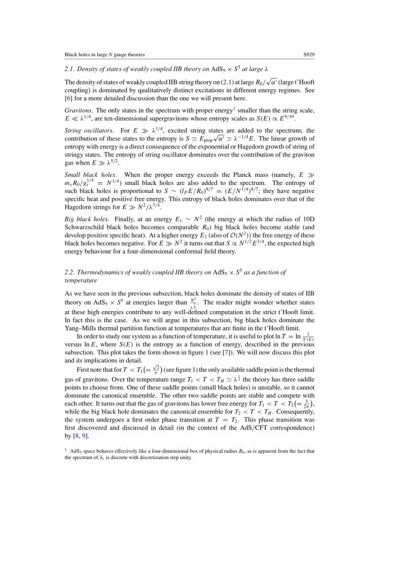
In order to study our system as a function of temperature, it is useful to plot ln T = ln 1S ′(E)

versus ln E, where S(E) is the entropy as a function of energy, described in the previoussubsection. This plot takes the form shown in figure 1 (see [7]). We will now discuss this plotand its implications in detail.

First note that for T < T1(= √

2π

)(see figure 1) the only available saddle point is the thermal

gas of gravitons. Over the temperature range T1 < T < TH � λ14 the theory has three saddle

points to choose from. One of these saddle points (small black holes) is unstable, so it cannotdominate the canonical ensemble. The other two saddle points are stable and compete witheach other. It turns out that the gas of gravitons has lower free energy for T1 < T < T2

(= 32π

),

while the big black hole dominates the canonical ensemble for T2 < T < TH . Consequently,the system undergoes a first order phase transition at T = T2. This phase transition wasfirst discovered and discussed in detail (in the context of the AdS/CFT correspondence)by [8, 9].

1 AdS5 space behaves effectively like a four-dimensional box of physical radius R0, as is apparent from the fact thatthe spectrum of ∂τ is discrete with discretization step unity.

S930 S Minwalla

Log(T_1)

Black HolesBig AdS

Gravitons

Small Black Holes

Hagedorn

Log(T_2)

= Log(T)

Log(S’(E))

Log(E) Log(E_1) Log(E_2)

−

Figure 1. log(T ) as a function of log(E) (in the microcanonical ensemble) for all the ‘phases’ oftype IIB string theory on AdS5 × S5, when R0 √

α′.

T = TH is the Hagedorn temperature beyond which the graviton gas saddle point doesnot exist. For T > TH the generic state of the theory continues to be a big black hole, the onlyphase available to the system at these temperatures.

3. Thermodynamics of N = 4 Yang–Mills in the limit λ → 0

The interesting thermal behaviour of weakly coupled IIB theory on a large radius AdS5 mustbe mirrored in the thermal partition function of N = 4 Yang–Mills theory at large λ. Thispartition function, while currently inaccessible at large λ, is easily computed in the oppositeweak coupling limit. The surprise is that, even in this apparently trivial limit, the system hasvery rich behaviour. In particular, it undergoes a sharp phase transition, strongly reminiscentof the phase transition to black hole nucleation, even in the free limit.

3.1. Setting up the computation

We choose to work in the gauge

∂iAi = 0, (3.1)

where i = 1, 2, 3 runs over the sphere coordinates, and ∂i are covariant derivatives. The choice(3.1) fixes the gauge freedom only partially; it leaves spatially independent but time-dependentgauge transformations unfixed. We fix this residual gauge invariance with the condition

∂tα(t) = 0, (3.2)

where

α ≡ 1

ω3

∫S3

A0, (3.3)

where ω3 is the volume of S3.The mode α will play a special role in what follows because it is the only zero mode

(mode whose action vanishes at quadratic order) in the decomposition of Yang–Mills theoryinto Kaluza–Klein modes on S3 × S1. Consequently, α fluctuations are strongly coupled atevery value of λ, including in the limit λ → 0. In particular, they cannot directly be integratedout in perturbation theory.

Black holes in large N gauge theories S931

In order to proceed with the perturbative evaluation of the partition function we will adopta two-step procedure. In the first step, discussed in this section, we integrate out all non-zeromodes2 and generate an effective action Seff(α) for α. As we will see Seff(α) is non-trivialeven at zero coupling and is further modified perturbatively in λ. Once we have obtainedSeff(α), we must then proceed to perform the integral over α using saddle point techniques(that are exact in the large N limit) in order to obtain Z(T ).

3.2. The integration measure

In this subsection we will define Seff(α) more carefully. Recall that the Yang–Mills free energymay be written as

e−βF =∫

dα

∫DA12 e−SYM(A,α), (3.4)

where 1 is the Fadeev Popov determinant conjugate to (3.1), 2 is the Fadeev Popovdeterminant conjugate to (3.2), and SYM is the Yang–Mills action. It is not difficult toexplicitly evaluate 2 (see later in this subsection) and verify that it is independent of A.Consequently, (3.4) may be rewritten as

e−βF =∫

dα2 exp[−Seff(α)], (3.5)

where

exp[−Seff(α)] =∫

DA1 exp[−SYM(A, α)]. (3.6)

In the rest of this subsection, we will explicitly evaluate 2 and so determine the effectivemeasure of integration (3.5).

It follows from (3.2) that

2 = det′ (∂0 − i [α, ∗]) , (3.7)

where the prime asserts that the determinant is over non-zero modes of A0. Denoting byλi (i = 1, . . . , n) the eigenvalues of α, and choosing a convenient basis of matrix functionswhose time dependence is given by exp(2π int/β), the determinant is easily evaluated as theproduct

2 =∏n�=0

∏i,j

[2π in

β− i(λi − λj )

]

=∏

m�=0

2π im

β

∏i,j

2

β(λi − λj )sin

(β(λi − λj )

2

). (3.8)

Notice that up to an overall constant,

dα2 = [dU ], (3.9)

where

dα =∏

i

dλi

∏i<j

(λi − λj )2 (3.10)

is the left–right invariant integration measure over Hermitian matrices α, and

[dU ] =∏

i

dλi

∏i<j

sin2

(β(λi − λj )

2

)(3.11)

2 As α is a zero mode this is a standard Wilsonian procedure.

S932 S Minwalla

is the left–right invariant integration measure in the integral over the unitary matrices

U ≡ eiβα. (3.12)

As we will see below, Seff may be regarded as a function of U rather than α, so that (3.5) maybe written as

e−βF =∫

[dU ] e−Seff(U) (3.13)

where Seff(U) is defined in (3.6).

3.3. Evaluation of Seff at one loop

The path integral in (3.5) may be evaluated diagrammatically, generating an expansion ofSeff(U) in powers of the gauge coupling. In this section we use this method to evaluate Seff(U)

to lowest order in λ (O(λ0)). This evaluation is rather simple as only one-loop graphs in theexpansion of (3.5) contribute to Seff at this order.

Although we are principally interested in N = 4 Yang–Mills theory, our computationsand results are very similar for all gauge theories. In order to keep things simple, we firstcompute Seff for pure gauge theories. The Fadeev–Popov determinant for gauge-fixing (3.1)is

det ∂iDi =

∫DcDc e−c∂iD

ic, (3.14)

where Di denotes a gauge covariant derivative

Dic = ∂i − i[Ai, c] (3.15)

and c and c are complex ghosts. Consequently, the action of the free gauge theory may bewritten as

e−Seff(U) =∫

DAiDA0DcDcδ(∂iAi) exp

[−∫

Tr

(1

2Ai(D

20 + ∂2)Ai +

1

2A0∂

2A0 + c∂2c

)],

(3.16)

where

D0X ≡ ∂0X − i[α,X]. (3.17)

To proceed further we note that any vector field on the sphere may be decomposed as

Ai = ∂iϕ + Bi (3.18)

where ∂iBi = 0. The integral over ϕ in (3.16) is easily performed using the δ function,

yielding 1/√

det′(∂i∂i) where the derivatives act on scalar functions on S3 and the primedenotes omission of the zero mode. The integral over A0 yields the identical factor (the zeromode is α which is not integrated over). The integral over the ghosts, on the other hand,evaluates to det′(∂i∂

i). These three factors cancel nicely, so that (3.16) simplifies to

e−Seff(U) =∫

DBi exp

[−1

2

∫Tr

(Bi

(D2

0 + ∂2)Bi)]

. (3.19)

Thus,

Seff = 12 ln

(det

(−D20 − ∂2

)), (3.20)

where the operator acts on the space of divergenceless vector functions on the sphere, i.e. thespace of vector functions spanned by the vector spherical harmonics. Consequently

Seff = 1

2

∑

n() ln det(−D2

0 + 2), (3.21)

Black holes in large N gauge theories S933

where 2 are the eigenvalues of the Laplacian acting on vector spherical harmonics on thecompact manifold and n() is the degeneracy of each eigenvalue. When the compact spaceis an S3 of unit radius we have = h + 1 (for integer h � 0) and n() = 2h(h + 2) ( see [3]for more on vector spherical harmonics).

The determinant of(−D2

0 +2)

is easily evaluated by passing to Fourier space in the timedirection, yielding the infinite product

detU(N)

[ ∞∏n=−∞

(4π2n2

β2+

4πn

βα + α2 + 2

)]. (3.22)

The infinite product of matrices may be rewritten as

(α2 + 2)

∏m�=0

β

2πm

−2 ∏n�=0

(1 +

βα

πn+

(α2 + 2)β2

4π2n2

)= (α2 + 2)

∏m�=0

β

2πm

−2 [ ∞∏n=1

(1 − β2(α + i)2

4π2n2

)(1 − β2(α − i)2

4π2n2

)]

=∏

m�=0

β

2πm

−2 (4

β2

)sin

[β(α + i)

2

]sin

[β(α − i)

2

]

= 2

β2

∏m�=0

β

2πm

−2

[cosh(β) − cos(βα)]

= N eβ(1 − e−β+iβα)(1 − e−β−iβα), (3.23)

where

N =

1

β2

∏m�=0

β

2πm

−2 . (3.24)

The divergent factor N is a constant independent of both and α, and we set it to unityto reproduce the free energy of the harmonic oscillator. Thus

ln(det

(−D20 + 2

)) = Tr(β + ln(1 − e−β+iβα) + ln(1 − e−β−iβα)), (3.25)

where the trace is over N2 ×N2-dimensional matrices and α acts in the adjoint representation.Expanding the logarithms in a power series, summing over , and passing from the adjoint tothe fundamental (Tr adj(einβα) → tr(Un) tr(U−n)) and using (3.20) we obtain

Seff = 1

2βN2

∑

n() −∞∑

n=1

zV (xn)

ntr(Un) tr(U−n) (3.26)

where zV (x) = 6x2−2x3

(1−x)3 is the trace of xE over the set of all vector spherical harmonics on S3.3

We will find it useful below to note that the equation zV (x) = 1 is solved at x = xH = 2−√3.

The corresponding temperature, TH = −1/ ln(2 − √3) � 0.759 326.

We now turn to the computation of Seff in theN = 4 Yang–Mills theory (our considerationsare very simply generalized to arbitrary free gauge theories). It is a simple matter to include

3 For the case of an S3 of unit radius the first term (appropriately regularized) is equal to 11120 βN2, where 11

120 is theCasimir energy

∑∞0 h(h + 1)(h + 2) for a vector field on the unit sphere.

S934 S Minwalla

the contributions from free conformally coupled scalar and spinor fields to our computations.When the compact manifold is S3, the contribution to Seff from a single additional scalar fieldis

δSeff = 12 ln

(det

(−D20 − ∂2 + 1

)), (3.27)

where the operator acts on scalar fields on S3 × S1 and the constant piece of the operator is aconsequence of the Rϕ2 term in the Lagrangian for conformally coupled scalars. As above,this determinant is easily evaluated to yield

Seff = 1

240βN2 −

∞∑n=1

zS(xn)

ntr(Un) tr(U−n), (3.28)

where 1240 = 1

2

∑∞n=0(n + 1)3 and zS(x) = x+x2

(1−x)3 is the partition function over scalar spherical

harmonics on S3. A Weyl spinor field on S3 contributes4

Seff = −ln(det(−∂0γ0 − ∂/)) = 17

960βN2 −

∞∑n=1

(−1)n+1zFW(xn)

ntr(Un) tr(U−n), (3.29)

where zFW(x) = 4x32

(1−x)3 and 17960 = −∑∞

n=1 n(n + 1)(n + 1

2

).

As the N = 4 Yang–Mills theory has one vector, six scalar and four Weyl fermion fields,the effective action for that theory is given by

Seff =∞∑

n=1

[zB(xn) − (−1)nzF (xn)]Tr UnTr U−n

n(3.30)

where zB(x) = zV (x) + 6zS(x) = 6x+12x2−2x3

(1−x)3 and zF (x) = 4zFW(x) = 16x32

(1−x)3 . Below we will

find it useful to note that zB(xH ) + zF (xH ) = 1 at xH = 7 − 4√

3, TH = −1/ ln(7 − 4√

3) �0.379 663.

This completes our derivation of Seff for N = 4 Yang–Mills theory in the limit λ → 0.We will now turn to the evaluation of the integral over the ‘Polyakov loop’ U.

3.4. Solution of the free Yang–Mills unitary integral: generalities

In this section we proceed to directly analyse the unitary matrix model (3.13) for the exactpartition function of free U(N) Yang–Mills theory in order to extract its thermodynamicbehaviour. (3.13) was first obtained by [1] using different techniques to those adopted in theprevious subsection. Although we are principally interested in N = 4 Yang–Mills theory,it turns out that all Yang–Mills theories with purely adjoint matter content display similarbehaviour; we will analyse all these theories together.

We begin by recalling that any unitary matrix model with gauge-invariant action andmeasure may be rewritten entirely in terms of the eigenvalues of the unitary matrix, whichmust lie on the unit circle. Denoting these eigenvalues by {eiαi } (with −π < αi � π ), we mayrewrite the partition function (3.13) in terms of the eigenvalues by the replacements∫

[dU ] →∏

i

∫ π

−π

[dαi]∏i<j

sin2

(αi − αj

2

), tr(Un) →

∑j

einαj . (3.31)

With only adjoint matter, we find from (3.13) that the effective theory for the eigenvalues isgoverned entirely by a pairwise potential,

4 We take the spinor field to be anti-periodic on the S1 in order to compute the trace of e−βH rather than the trace of(−1)F e−βH .

Black holes in large N gauge theories S935

Z(x) =∫

[dαi] e−∑i �=j V (αi−αj ) (3.32)

where

V (θ) = −ln|sin(θ/2)| −∞∑

n=1

1

n[zB(xn) + (−1)n+1zF (xn)] cos(nθ)

= ln(2) +∞∑

n=1

1

n(1 − zB(xn) − (−1)n+1zF (xn)) cos(nθ). (3.33)

In the first line, the first term coming from the measure is a temperature-independent repulsivepotential, while the remaining terms provide an attractive potential which increases from zeroto infinite strength as the temperature increases from zero to infinity.5 This suggests that at lowtemperatures, the minimum action configurations will correspond to eigenvalues distributedevenly around the circle, while at high temperatures, the eigenvalues will tend to bunch up.

For finite N, the partition function receives contributions from all configurations ofeigenvalues and depends smoothly on the temperature. On the other hand, it is well knownthat in the large N limit, the matrix model partition function is dominated by the minimumaction configurations, with the exact leading and subleading terms in the 1/N expansion ofthe free energy given, respectively, by the minimum of the action and by the Gaussian integralabout the minimum action configuration. When this minimum action configuration (or itsderivatives) changes abruptly as a function of temperature, we may have a phase transition inthe large N limit (see, for example, [10]). We will now see that exactly this behaviour occursand leads to a phase transition for our model.

3.5. Low temperature behaviour of the unitary integral

Consider first the theory at low temperatures, where the effective potential between theeigenvalues is dominated by the repulsive term. In this case, we expect that the pairwiserepulsion drives the eigenvalues to spread uniformly around the circle. In fact, since thereis no difference between displacing any individual eigenvalue in the uniform distribution tothe left and displacing it to the right, the uniform eigenvalue distribution will always be astationary point of the action for a pairwise potential. To see when this stationary point isa minimum, it is convenient to introduce an eigenvalue distribution ρ(θ) proportional to thedensity of eigenvalues eiθ of U at the point θ . Note that ρ must be everywhere non-negative,and we may choose its normalization so that∫ π

−π

dθρ(θ) = 1. (3.35)

With this definition, the effective action for the eigenvalues becomes

S[ρ(θ)] = N2∫

dθ1

∫dθ2ρ(θ1)ρ(θ2)V (θ1 − θ2)

= N2

2π

∞∑n=1

|ρn|2Vn(T ), (3.36)

5 To see that the second term in the potential is always attractive, note that we may rewrite it as

V2(θ) = 1

2

∫dE{ρB(E) ln(1 − 2xE cos(θ) + x2E) − ρF (E) ln(1 + 2xE cos(θ) + x2E)}, (3.34)

where ρB and ρF give the single-particle density of states for bosonic and fermionic modes . This potential is alwaysattractive since for any value of E and x the integrand is decreasing in the interval θ ∈ [−π, 0] and increasing in theinterval θ ∈ [0, π ].

S936 S Minwalla

where in the second line, we have defined ρn ≡ ∫dθρ(θ) cos(nθ) and Vn ≡ ∫

dθV (θ) cos(nθ)

to be the Fourier modes on the circle of ρ and V , respectively, and we assume without lossof generality that the eigenvalue distribution is symmetric around θ = 0. From the latterexpression, it is clear that the uniform distribution (ρn�1 = 0) will be an absolute minimumof the potential as long as all Vn are positive. From (3.33) we see that

Vn = 2π

n(1 − zB(xn) − (−1)n+1zF (xn)), (3.37)

so the uniform distribution is an absolute minimum if and only if

zB(xn) + (−1)n+1zF (xn) < 1 (3.38)

for all n. But, since the single-particle partition functions are monotonically increasing, and0 � x < 1, the n = 1 condition is always strongest, and the uniform distribution will be stablefor temperatures T < TH = −1/ ln(xH ) where xH is the solution to

z(xH ) ≡ zB(xH ) + zF (xH ) = 1, (3.39)

xH and TH were determined for pure Yang–Mills and N = 4 Yang–Mills behind; as wewill see below, the temperature TH may be thought of as both a phase transition and aHagedorn temperature. As long as we have more than a single quantum-mechanical mode,equation (3.39) always has a unique solution with 0 < x < 1, so the uniform distributionbecomes an unstable extremum beyond some finite temperature TH determined by the single-particle partition function.

For T < TH , we may now evaluate the free energy at leading and subleading order in N.Since tr(Un) vanishes for any n � 1 for the uniform distribution, the classical value for theaction (3.13) (and thus the leading O(N2) contribution to the free energy) vanishes. The firstnon-zero contribution to the free energy thus arises from the Gaussian integral around thisconfiguration. From the quadratic action (3.36), (3.37), we see that the leading contributionto the partition function is6

Z(x) =∞∏

n=1

1

1 − zB(xn) − (−1)n+1zF (xn), (3.40)

where the normalization has been arbitrarily fixed by choosing the vacuum free energy tovanish, Z(x = 0) = 1 (more physically, we could choose Z(0) to account for the Casimirenergy of the vacuum, see the previous subsection).

This partition function diverges at T = TH , as should be expected, since this is thepoint where the quadratic action (3.36) develops an unstable direction. The correspondingdivergence in the free energy F = −T ln(Z) goes like

F → TH ln(TH − T ) (3.41)

as T approaches TH from below. This divergence is associated with a Hagedorn density ofstates,

ρ(E) ∝ E0 eβH E. (3.42)

Thus, just as for perturbative string theory, the partition function free, large N Yang–Millstheory on S3 has a Hagedorn divergence which is associated with an unstable mode in theEuclidean path integral. The ‘tachyon’ that causes the divergence is the lowest ‘momentum’fluctuation mode ρ1 of the eigenvalues. In the next subsection, we will be able to see explicitlywhat the endpoint of this tachyon condensation brings as we raise the temperature beyond theHagedorn temperature.

6 The ‘Jacobian’ for the ‘change of variables’ from λi to ρn appears to be irrelevant at every order in the 1/N

expansion, see [11].

Black holes in large N gauge theories S937

3.6. Behaviour near the transition

At the temperature T = TH , V1 vanishes and the mode ρ1 (the lowest momentum fluctuation inthe eigenvalue distribution) becomes massless. Since the action is quadratic, this correspondsto an exactly flat direction in the potential, and the corresponding family of minimum actionconfigurations are given (up to overall translations of θ ) by

ρ(θ) = 1

2π(1 + t cos(θ)), 0 � t � 1, (3.43)

which interpolate between the uniform distribution and a sinusoid vanishing at a singlepoint. For T > TH , the quadratic form S has negative coefficients, so all minimum actionconfigurations must lie at the boundary of configuration space, at a point where a hyperboloidof constant S lies tangent to this boundary. Since this boundary is provided by the positivitycondition ρ(θ) � 0, these minimum action eigenvalue distributions necessarily vanish on asubset of the circle.

In the limit of small, positive T = T − TH , the action contour S = 0 is a cone withopening angle going to zero. The contours of smaller S are hyperboloids inside this cone,so the minimum action configuration lies on the boundary of the configuration space insidethe cone. Finally, it is easy to see that the region of allowed ρ’s is convex (if points {ρn}and {ρ ′

n} are in the region then all points {tρn + (1 − t)ρ ′n} are in the region for 0 � t � 1).

Thus, the boundary region interior to the cone is a simply-connected neighbourhood of thet = 1 configuration in (3.43) whose size goes to zero as T → TH . We conclude that theminimizing configuration changes continuously from the t = 1 configuration in (3.43) for Tin some interval above TH .

The leading behaviour of the free energy in this vicinity of TH is then given by evaluatingthe V1 term in the action (3.36) on the t = 1 configuration in (3.43), since the effects ofchanging the eigenvalue distribution come in at higher orders.

Thus, the leading result for the minimum action is

SminT >TH

(x) = N2

8π(T − TH )V ′

1(TH ) + · · · (3.44)

from which we may obtain the free energy as F = T Smin. The leading behaviour near thetransition is therefore given by

limN→∞

1

N2FT →TH

(T ) =0 T < TH

−1

4(T − TH )z′(xH )

xH

TH

T > TH

(3.45)

so we have a first order phase transition at the Hagedorn temperature. Note also that thebehaviour is characteristic of a deconfinement transition, since the free energy is O(1) belowthe transition and O(N2) above the transition. This will be verified in section 5.7 below whenwe discuss the behaviour of a second order parameter for confinement, related to the Polyakovloop.

3.7. High temperature behaviour

For general values of T > TH , we will not be able to write down an exact expression for the freeenergy (though it is possible to generate a perturbation series for the solution, in T − TH thatmay be used to evaluate the free energy to arbitrary accuracy). However, the theory simplifiesagain in the large temperature limit, where the potential becomes strongly attractive7. In

7 The high temperature regime and its relation to string theory was discussed for uncompactified theories in [12] in avery similar language to the one we are using here, and this discussion was applied to two-dimensional QCD in [13]

S938 S Minwalla

N

2lim (F/N )

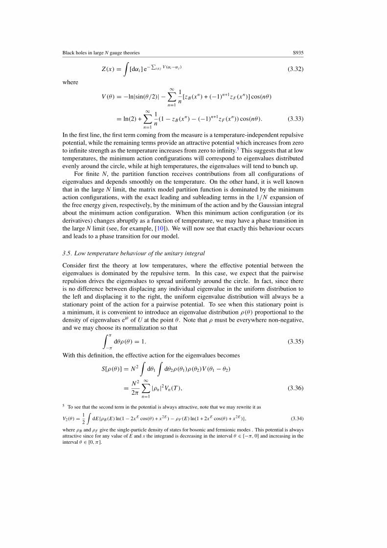
TTH

Figure 2. Free energy as a function of temperature in free Yang–Mills theories.

this case, the action is minimized by a tightly clustered configuration of eigenvalues thatapproaches a delta function in the limit of infinite temperature. Thus, we should have ρn = 1to leading order, and

S = N2

2π

∞∑n=1

Vn(T 1). (3.46)

The high temperature limit of the single-particle partition functions depends only on thespace-time dimension d and the number of physical polarizations N dof of the fields in thetheory,

zi(x) → 2N dofi T d−1 + O(T d−2). (3.47)

Using (3.37), we find that the high temperature limit of the free energy is

F(x → 1) = −2N2T dζ(d)

[N dof

B +

(1 − 1

2d−1

)N dof

F

]+ O(T d−1). (3.48)

The limiting free energy density here coincides with that of the flat space theory, which shouldbe expected since in the free field analysis we are dealing with a scale-invariant theory, sotaking the dimensionless temperature T R to infinity is equivalent to taking the limit of largevolume at fixed temperature (see [14–16] among others for the high temperature expansion ofthe free energy for the U(1) theory).

3.8. Summary of thermodynamic behaviour as for λ → 0

We are now in a position to present a reasonably detailed picture of the behaviour of the freeenergy of the free gauge theory at all temperatures, depicted in figure 2.

We find that the uniform eigenvalue distribution provides an absolute minimum of thematrix model potential for all temperatures below some TH determined by the single-particlepartition function as

z(TH ) = 1. (3.49)

The free energy in this regime, given by (3.40), is O(1) and decreases monotonically to alogarithmic divergence (3.41) at T = TH , characteristic of a Hagedorn density of states (3.42).

As T increases past TH , the uniform eigenvalue distribution develops an unstable modewhich condenses to give a pure sinusoid distribution (3.43) for T just above TH , and adistribution with a gap for T > TH . For small (T − TH ), the O(N2) free energy decreases

Black holes in large N gauge theories S939

linearly in T − TH , so the first derivative of the free energy is discontinuous and we have afirst order phase transition. Although we have not described this here, the free energy as afunction of temperature may be written as a perturbation expansion in T − TH [2].

In the high temperature limit, the pairwise potential between eigenvalues becomes stronglyattractive, and the eigenvalue distribution approaches a delta function. In this regime, thefree energy asymptotes to (3.48) which corresponds to the expected flat-space free-energydensity. It is possible to work out the high temperature behaviour as a perturbation expansionin 1/T [2].

3.9. Comparison with λ → ∞At both λ → ∞ and λ → 0,N = 4 Yang–Mills theory undergoes a single first order phasetransition at a temperature of order unity. In both limits, the low and high temperature phase aredistinguished by the same order parameters; F/N2 (where F is the free energy) and Tr U/N 8

are both non-zero in the high temperature phase but zero in the low temperature phase.Despite these similarities, thermodynamics at λ = 0 and λ = ∞ are different in one

important respect. The phase transition at λ = ∞ results from a competition between twodifferent phases, each of which is metastable over an open set of temperatures that includesthe phase transition temperature. In this range of temperatures the system also possesses athird, unstable, saddle point. On the other hand at λ = 0 the low temperature phase is unstableabove the phase transition temperature, while the high temperature phase is unstable belowthis temperature (so that we never have more than one stable phase at any temperature) ; andwe have seen no sign of a third saddle point.

As we will explain in the next section, these differences all a consequence of the factthat Seff in Free Yang–Mills theory is extremely finely tuned. In particular it is an exactlyquadratic function of the order parameter u1. Yang–Mills interactions do not preserve thisspecial feature of Seff , and thus modify the detailed nature of thermodynamics in a qualitativefashion.

4. Turning on the coupling constant

In this section we will investigate how λ → 0 thermodynamics, for any Yang–Mills theory onS3 (including the N = 4 theory) is modified by coupling constant effects.

4.1. Exact constraints on Seff from gauge invariance

Gauge invariance imposes tight constraints on the form of the effective action Seff(α) (3.6)for the zero mode of the gauge field; Seff(α) should be invariant under all space-time gaugetransformations that

(1) are single valued (up to an element of the centre of U(N)) on M × S1,(2) preserve the gauge-fixing conditions (3.1) and (3.2).

We will restrict attention to gauge transformations U(t) that are independent of theposition on the compact space. Under such a transformation

A0 → V (t)A0V†(t) − i∂tV V †, (4.1)

so that

α → V (t)αV †(t) − i∂tV V †. (4.2)

8 The second order parameter is a little subtle; see [2] for a discussion of this point.

S940 S Minwalla

V (t) obeys the condition (2) above (and (4.2) makes sense) only when the right-hand side of(4.2) is independent of time.

Constant (time independent) gauge transformations clearly satisfy the requirements (1)and (2) above. Consequently, Seff(α) is invariant under α → V αV †. We may use thisinvariance to diagonalize α. Once this has been done, we consider the further gaugetransformations

V (t) = eitD, (4.3)

where D is a diagonal matrix, whose eigenvalues are all integral multiples of 2π/β. α

transforms under the gauge transformation generated by (4.3) as α → α + D. This impliesthat Seff(α) is invariant under separate shifts of any of the eigenvalues of α by multiples of2π/β. It follows from these invariances that Seff is really a function only of tr(Un) (for all n)where U = eiβα (see equation (3.12)) is the zero mode holonomy around the time circle.

Finally, consider V (t) = e2π iktβN where k is an integer if the gauge group is SU(N), and

arbitrary for U(N). V (t) obeys the single-valuedness condition (1), as e2π ikN belongs to the

centre of the gauge group. Under the gauge transformation generated by V (t), α → α + 2πkNβ

.

Consequently, Seff should be invariant under U → e2πikN U , for all integers k if the gauge group

is SU(N), and for any k for U(N). In the limit N → ∞ the two cases coincide, and Seff(U)

must be invariant under U → eiθU for arbitrary θ . Putting everything together, we concludethat Seff may depend on U only in combinations of the form

tr(Un1) · · · tr(Unk ) tr(U−n1−···−nk ). (4.4)

4.2. The general form of the effective action in perturbation theory

In large N perturbation theory, Seff is generated by planar vacuum diagrams obtained byintegrating out the massive modes. In this calculation, α is a background field, which appearsdiagrammatically via external line insertions on the index loops of diagrams. Planar diagramsat order λk−1 include (k+1) index loops, each of which leads to a trace in the final result (whichmay contain arbitrarily many factors of α). From the discussion of the previous subsection,the only terms with (k + 1) traces allowed by gauge invariance take the form (4.4). It followsthat the most general form of the planar contribution to Seff in perturbation theory is

Seff(U) = N2

[∑n

m2n(x)|un|2 + λ

∑m,n

Fm,n(x)(umunu−n−m + c.c.)

+ λ2∑m,n,p

Fm,n,p(x)(umunupu−m−n−p + c.c.) + · · ·], (4.5)

where we have defined un ≡ tr(Un)/N (note that u∗n = u−n and u0 = 1). This agrees, of

course, with the quadratic form of the one-loop effective action that we found in sections 3and 4. Also, the un coincide with the variables ρn used in section 5 for eigenvalue distributionswhich are symmetric about θ = 0, so the values of m2

n in the free field theory may be read offfrom equation (3.37).

4.3. Possible phase structures at weak coupling

Recall that at λ = 0, u1 is massless at the phase transition temperature TH , while the other un’sare all massive. Consequently, u1 will continue to be the lightest mode in the vicinity of thephase transition at weak coupling. Thus, for analysing the phase transition at weak coupling, itis useful to obtain an effective action for u1 by integrating out the un’s with n > 1.9 It follows9 As we are interested in the large N limit, it is sufficient to integrate out these modes classically.

Black holes in large N gauge theories S941

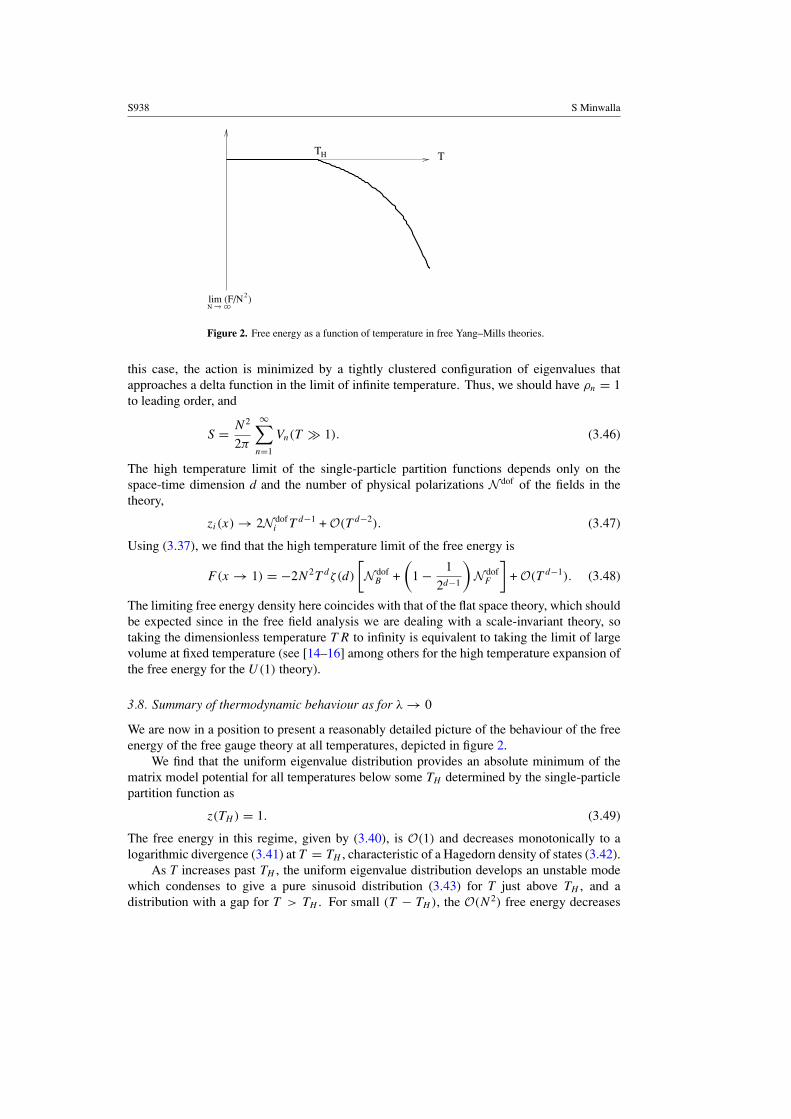
from (4.5) that the leading large N terms in the resulting effective action are of the form

Seff(u1) = N2

(m2

1(x, λ)|u1|2 +∞∑

n=2

λ2n−2Bn(x, λ)|u1|2n

), (4.6)

where m21 and the Bn’s are functions of the temperature and power series in λ starting

(generically) from a λ0 term.In particular to O(λ2), we have

Seff(u1) = N2 (m21|u1|2 + b|u1|4

), (4.7)

where b(x) = B2(x, 0)λ2 is a function of temperature which is generically non-zero. It is notdifficult to compute B2(0) starting from (4.5). The only terms in (4.5) that contribute are

S ′eff(U) = N2 (m2

1|u1|2 + m22|u2|2 + λI

(u−2u

21 + u2u

2−1

)+ λ2A|u1|4

). (4.8)

At this order, u2 may be integrated out from (4.8) by setting it to be equal to its classicalvalue u2 = −Iλu2

1

/m2

2,10 yielding (4.7) with b = (A − I 2

/m2

2

)λ2. Note that because the

eigenvalue density (4.9) has to be non-negative everywhere, our expressions for the effectiveaction (4.6) and (4.7) are valid only for u1 such that |u1| � 1

2 + O(λ).As in the previous section, the one-loop contribution to the free energy coming from

integrating over u1 diverges at the temperature TH (λ) at which m21(x, λ) goes to zero and u1

becomes massless. For any value of the coupling, at leading order in the distance from thistemperature, we have m2

1 � K(TH (λ) − T ) for some positive constant K. This divergencesignals a Hagedorn behaviour of the single-particle spectrum of the theory with Hagedorntemperature TH (computable in perturbation theory), so this behaviour persists (at least in themicrocanonical ensemble) even at non-zero t’Hooft coupling.

As the saddle point at u1 = 0 is unstable for T > TH , the theory described by (4.7)clearly undergoes a phase transition (to another saddle point) at some T � TH . Whetherthis phase transition occurs at T < TH or T = TH depends on whether the value of b(defined in (4.7)) at the Hagedorn temperature TH is positive or negative, as we now argue indetail11. The formulae in the remainder of this section are all correct only to leading order in b(or in λ).

First, consider the case b > 0. For T < TH , u1 = 0, corresponding to the uniformeigenvalue distribution, is clearly a global minimum of the effective action (4.7). For T > TH ,however, u1 = 0 is unstable and Seff is minimized at |u1|2 = |m1|2/2b. The value of theeffective action at this minimum is Seff = −N2|m1|4/4b, which is of order (T − TH )2, andso the phase transition at T = TH is of second order. As the temperature is raised aboveTH , the eigenvalue distribution smoothly becomes non-uniform until we reach |u1|2 = 1/4;this occurs at m2

1 = −b/2. At this point, ρ(θ) vanishes at some θ and we have reached theboundary of the space of eigenvalue distributions and the edge of the validity of (4.7). Asthe temperature is further raised the eigenvalue distribution develops a gap on the circle, andthe theory undergoes a further phase transition similar to the Gross–Witten transition [10].This second phase transition (at T = TH + b

2K) is of third order. The behaviour above this

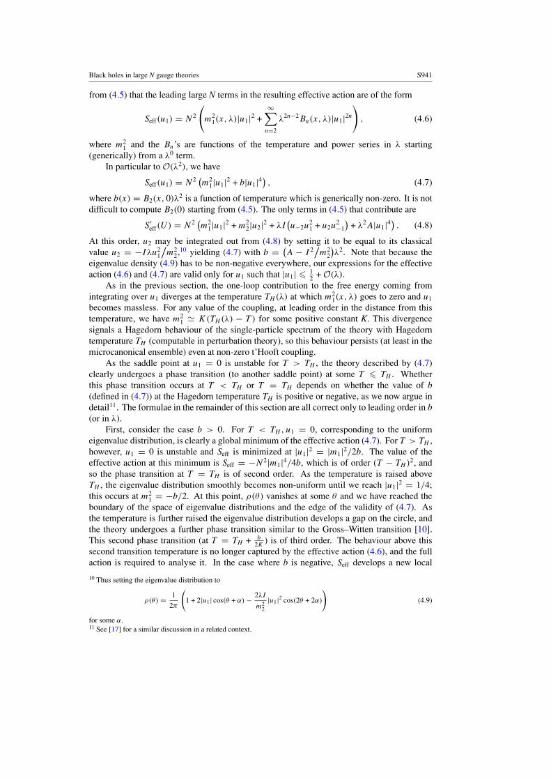
second transition temperature is no longer captured by the effective action (4.6), and the fullaction is required to analyse it. In the case where b is negative, Seff develops a new local

10 Thus setting the eigenvalue distribution to

ρ(θ) = 1

2π

(1 + 2|u1| cos(θ + α) − 2λI

m22

|u1|2 cos(2θ + 2α)

)(4.9)

for some α.11 See [17] for a similar discussion in a related context.

S942 S Minwalla

0.1 0.2 0.3 0.4 0.5

-0.125

-0.1

-0.075

-0.05

-0.025

0.025

0.05

Figure 3. Plots of Seff(u1) as a function of u1 for small positive b, in units of N2b, at severalvalues of m2

1 (from top to bottom) : m21 = 0 (Hagedorn temperature and first phase transition

temperature), m21 = − b

4 , m21 = − b

2 (second phase transition temperature), and m21 = − 3b

4 .

0.10.20.30.40.5

-0.025

0.025

0.05

0.075

0.1

0.125

Figure 4. Plots of Seff(u1) as a function of u1 for small negative b, in units of N2|b|, at severalvalues of m2

1 (from top to bottom) : m21 = 3|b|

4 , m21 = |b|

2 (new phase nucleated), m21 = |b|

4 (first

order phase transition temperature), m21 = |b|

8 , and m21 = − |b|

8 .

minimum at |u1| = 12 (the boundary of our order parameter space) when m2

1 < |b|/2; notethis happens below the Hagedorn temperature. When m2

1 > |b|/4, the free energy at thisnew local minimum is positive, and the saddle point |u1| = 1

2 is disfavoured compared tou1 = 0. However, when we raise the temperature to m2

1 < |b|/4, the free energy at |u1| = 12

becomes negative, and so this saddle dominates over the u1 = 0 saddle point. Consequently,at T = TH − |b|

2K, |u1| jumps discontinuously from zero to 1

2 and the theory undergoes a firstorder phase transition. When the temperature is further raised, the eigenvalue distributiondevelops a break on the circle and the theory is no longer described by (4.6). This behaviouris qualitatively similar to that of the free theory which we analysed in section 5, except thatthe phase transition now happens below the Hagedorn temperature TH .

If b vanishes exactly then the higher order terms in (4.6) are required for analysingthe phase transition, but generically b will not vanish at the Hagedorn temperature. In

Black holes in large N gauge theories S943

TR

PHASE III

λ

Hagedorn Temperature

PHASE I

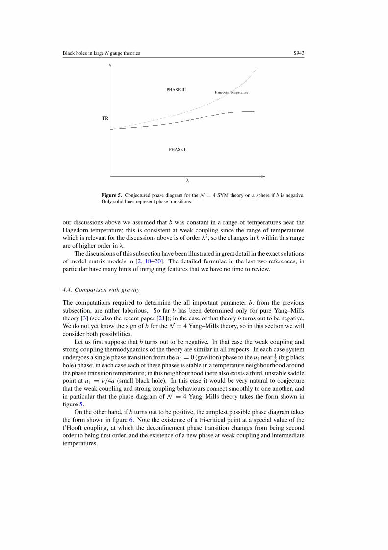
Figure 5. Conjectured phase diagram for the N = 4 SYM theory on a sphere if b is negative.Only solid lines represent phase transitions.

our discussions above we assumed that b was constant in a range of temperatures near theHagedorn temperature; this is consistent at weak coupling since the range of temperatureswhich is relevant for the discussions above is of order λ2, so the changes in b within this rangeare of higher order in λ.

The discussions of this subsection have been illustrated in great detail in the exact solutionsof model matrix models in [2, 18–20]. The detailed formulae in the last two references, inparticular have many hints of intriguing features that we have no time to review.

4.4. Comparison with gravity

The computations required to determine the all important parameter b, from the previoussubsection, are rather laborious. So far b has been determined only for pure Yang–Millstheory [3] (see also the recent paper [21]); in the case of that theory b turns out to be negative.We do not yet know the sign of b for the N = 4 Yang–Mills theory, so in this section we willconsider both possibilities.

Let us first suppose that b turns out to be negative. In that case the weak coupling andstrong coupling thermodynamics of the theory are similar in all respects. In each case systemundergoes a single phase transition from the u1 = 0 (graviton) phase to the u1 near 1

2 (big blackhole) phase; in each case each of these phases is stable in a temperature neighbourhood aroundthe phase transition temperature; in this neighbourhood there also exists a third, unstable saddlepoint at u1 = b/4a (small black hole). In this case it would be very natural to conjecturethat the weak coupling and strong coupling behaviours connect smoothly to one another, andin particular that the phase diagram of N = 4 Yang–Mills theory takes the form shown infigure 5.

On the other hand, if b turns out to be positive, the simplest possible phase diagram takesthe form shown in figure 6. Note the existence of a tri-critical point at a special value of thet’Hooft coupling, at which the deconfinement phase transition changes from being secondorder to being first order, and the existence of a new phase at weak coupling and intermediatetemperatures.

S944 S Minwalla

Hagedorn

HagedornPHASE II

PHASE III

PHASE I

λ

TR

Figure 6. Conjectured phase diagram for the N = 4 SYM theory on a sphere if b is positive. Onlysolid lines represent phase transitions.

While the two possibilities above are different in detail, they share one important feature.In both cases the saddle point near u1 = 1

2 is the analytic continuation, to weak coupling, ofthe big black hole saddle point.

It certainly seems possible that puzzling features of classical gravity, such as the existenceof singularities or the Hawking information puzzle, persist to all orders in the α′ expansion, butare resolved by quantum effects. If this is indeed the case, it should be possible to formulatea computation in weakly coupled Yang–Mills, whose result would explain the resolution ofthese paradoxes.

4.5. An aside: phase diagram of pure Yang–Mills theory as a function of �QCDR andtemperature

Pure Yang–Mills theory on an S3 or radius R has an effective coupling constant, givenby a monotonic function of �QCDR. As we have explained above, b is negative for thistheory. Further, lattice studies demonstrate that this theory undergoes a single first order phasetransition, at a temperature of order �QCD, at infinite R�QCD. Putting these two pieces of datatogether, it is natural to conjecture that the phase diagram of pure Yang–Mills theory takes theform shown in figure 7.

We have no understanding of the extreme right end of figure 7 (in fact a demonstrationthat the deconfinement transition, on that diagram, occurs at a temperature of order �QCD isliterally a million dollar question). On the other hand the LHS of the same diagram is underperfect analytic control. We thus see that putting pure Yang–Mills on a sphere adds a new axisto the problem of confinement in Yang–Mills theory, one that at least provides a new startingpoint for an analytic expansion of this challenging problem.

5. Black holes in the gravity duals to confining gauge theories

In this section, and for the rest of these lectures, we completely shift gears. We turn to a studyof black holes—and the gauge theoretic interpretation thereof—in gravity duals to confininggauge theories.

Black holes in large N gauge theories S945

RΛ QCD

T R

PHASE I

PHASE III

Hagedorn Temperature

Figure 7. The simplest phase diagram for a compactified confining theory with negative b and afirst order phase transition at R = ∞ . Only solid lines represent phase transitions.

As we will see below, the black holes we will consider below are more interesting thanbig black holes in AdS space from some points of view. Black holes in AdS5 are stable (theyare in thermal equilibrium with their Hawking radiation). Further, they exist in a theory withno asymptotic states. For both these reasons it is not possible to discuss the formation ofthese black holes via scattering and their subsequent decay via Hawking radiation. The blackholes we study below can easily be studied created by scattering; they subsequently decayvia Hawking radiation. We will pay a price for these new interesting features; the dual gaugedynamics that captures these black holes will turn out to be always strongly coupled, and sowill be under only qualitative control.

5.1. The Gravitational background under study

Consider the space

ds2 = L2α′(

e2u(−dt2 + T2π (u) dθ2 + dw2

i

)+

1

T2π (u)du2

)+ ds2

M, (5.1)

where i = 1, . . . , d − 1, θ ≡ θ + 2π and

Tx(u) = 1 −( x

4π(d + 1)eu

)−(d+1)

. (5.2)

This metric, known as the AdS soliton [22], is a solution to the d + 2-dimensional Einsteinequations with a cosmological constant

Rµν = −d + 1

L2α′ gµν, (5.3)

and has a simple physical interpretation [9]. It may roughly be thought of as a Scherk–Schwarzcompactification of AdSd+2 on a circle. Indeed, at large u, Tx(u) � 1 and (5.1) reduces toAdSd+2 in Poincare-patch coordinates, with u as the radial scale coordinate, and with oneof the spatial boundary coordinates, θ , compactified on a circle (the remaining boundarycoordinates, wi and t, remain non-compact). At smaller values of u, (5.1) deviates fromthe metric of periodically identified AdSd+2. In particular the θ circle shrinks to zero atu = u0 = −ln(d + 1)/2, smoothly cutting off the IR region of AdSd+2.

S946 S Minwalla

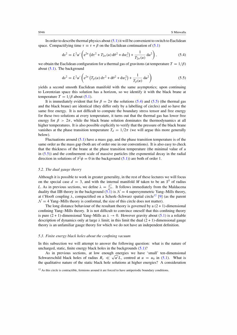
In order to describe thermal physics about (5.1) it will be convenient to switch to Euclideanspace. Compactifying time τ ≡ τ + β on the Euclidean continuation of (5.1)

ds2 = L2α′(

e2u(dτ 2 + T2π (u) dθ2 + dw2

i

)+

1

T2π (u)du2

), (5.4)

we obtain the Euclidean configuration for a thermal gas of gravitons (at temperature T = 1/β)about (5.1). The background

ds2 = L2α′(

e2u(Tβ(u) dτ 2 + dθ2 + dw2

i

)+

1

Tβ(u)du2

)(5.5)

yields a second smooth Euclidean manifold with the same asymptotics; upon continuingto Lorentzian space this solution has a horizon, so we identify it with the black brane attemperature T = 1/β about (5.1).

It is immediately evident that for β = 2π the solutions (5.4) and (5.5) (the thermal gasand the black brane) are identical (they differ only by a labelling of circles) and so have thesame free energy. It is not difficult to compute the boundary stress tensor and free energyfor these two solutions at every temperature, it turns out that the thermal gas has lower freeenergy for β > 2π , while the black brane solution dominates the thermodynamics at allhigher temperatures. It is also possible explicitly to verify that the pressure of the black branevanishes at the phase transition temperature Td = 1/2π (we will argue this more generallybelow).

Fluctuations around (5.1) have a mass gap, and the phase transition temperature is of thesame order as the mass gap (both are of order one in our conventions). It is also easy to checkthat the thickness of the brane at the phase transition temperature (the minimal value of uin (5.5)) and the confinement scale of massive particles (the exponential decay in the radialdirection in solutions of ∂2φ = 0 in the background (5.1)) are both of order 1.

5.2. The dual gauge theory

Although it is possible to work in greater generality, in the rest of these lectures we will focuson the special case d = 3, and with the internal manifold M taken to be an S5 of radiusL. As in previous sections, we define λ = L4

α′2 . It follows immediately from the Maldacenaduality that IIB theory in the background (5.1) is N = 4 supersymmetric Yang–Mills theory,at t’Hooft coupling λ, compactified on a Scherk–Schwarz spatial circle12 [9] (as the parentN = 4 Yang–Mills theory is conformal, the size of this circle does not matter).

The long distance behaviour of the resultant theory is governed by a (2 + 1)-dimensionalconfining Yang–Mills theory. It is not difficult to convince oneself that this confining theoryis pure (2 + 1)-dimensional Yang–Mills as λ → 0. However gravity about (5.1) is a reliabledescription of dynamics only at large λ limit; in this limit the dual (2 + 1)-dimensional gaugetheory is an unfamiliar gauge theory for which we do not have an independent definition.

5.3. Finite energy black holes about the confining vacuum

In this subsection we will attempt to answer the following question: what is the nature ofuncharged, static, finite energy black holes in the backgrounds (5.1)?

As in previous sections, at low enough energies we have ‘small’ ten-dimensionalSchwarzschild black holes of radius Rs � √

α′L, centred at u = u0 in (5.1). What isthe qualitative nature of the static black hole solutions at higher energies? A consideration

12 As this circle is contractible, fermions around it are forced to have antiperiodic boundary conditions.

Black holes in large N gauge theories S947

of the opposite, high energy limit gives us a clue. As we have seen above (5.1) hosts infiniteenergy translationally invariant (in the field theory R

2 directions) black brane solutions. Theseblack branes are clearly extensive (their energy and entropy are proportional to their volumein R

2). Further correlation functions of all fields in (5.1) decay exponentially in the R2

directions. Putting these statements together, it is natural to guess there exist large disc-shaped(in the in R

2 directions) black holes which, in their interior (meaning away from its edge ofthe disc) closely resemble a translationally invariant black brane. But a black brane at whattemperature? This question is easily answered by a ‘force balance’ argument, as we will nowpause to explain.

As we have reviewed in the appendix, gravitational theories in asymptotically AdS spaceshave well defined, conserved boundary stress tensors. In p spatial dimensions (p = 2 above,but it is just as easy to present the argument for general p) the equation ∇µTµr = 0, for staticconfigurations, reduces to

∂rTrr +1

r(pTrr − gijTij ) = 0, (5.6)

where i, j are summed over all spatial coordinates. When the effective gravitational fluid isisotropic (as is the case for black branes, and is approximately the case in the centre of ourdisc-like black holes) pTrr = gijTij , and any constant Trr solves (5.6). Near the edge of thedisc of our black hole, however, the stress tensor is not isotropic. Integrating (5.6) we find

Trr(∞) − Trr(0) = P(0) = −∫ ∞

0

dr

r(pTrr − gijTij ), (5.7)

where P(0) is the pressure in the centre of our disc. The integral on the right-hand side of(5.7) receives contributions only from the neighbourhood of the boundary of the disc. Weconclude that P(0) = p �′

rwhere

�′(r) = 1

p − 1

∫ ∞

0dr(gijTij − pTrr). (5.8)

The bubble walls of very large discs are well approximated by bubble walls of infinitely largediscs, and we find

�′(r) = � + O(

1

r

)� = 1

p − 1

∫ ∞

−∞dx gijTij =

∫ ∞

−∞dxTyy (5.9)

where x and y are Cartesian coordinates perpendicular and parallel to the disc, respectively.We find

P(0) = (p − 1)�

r+ O

(1

r2

). (5.10)

Now recall that P(Tc) = 0. Using the thermodynamic relation dPdT

= s (where s is the entropydensity) we find that the effective black brane temperature at the centre of the disc is given by

T (r) = Td +(p − 1)�

s(Td)× 1

r+ O

(1

r2

)(5.11)

where Td = 12π

is the phase transition temperature and s(Td) is a positive number, easilydetermined from the formulae of the appendix.

In summary, the intuition of the previous paragraphs suggests that there exist disc-shaped(in the R2 directions) finite energy black holes at all radii r 1 (1 is the length scale associatedwith the mass gap in this background) which in their interior are well approximated by blackbranes at temperature T (r) given by (5.11). The RHS of (5.11) contains a quantity, � that isa priori unknown. As a consequence a really sharp prediction that emerges from this discussion

S948 S Minwalla

only in the limit r → ∞; specializing our discussion to this limit we predict the existence of asolution, translationally invariant along the y direction, that interpolates between the vacuum(5.1) as x → −∞ and the black brane (5.5) at Td = 1

2pias x → ∞.

Although this solution has proven difficult to find analytically, it has been constructednumerically in [4]. Unfortunately this rather beautiful numerical construction is too intricateto describe here. It yields results precise enough to determine all the properties of this ‘domainwall’, including the positive domain wall tension �, and thus the RHS of (5.11) to within afew per cent. We take the existence of this domain wall solution as strong supporting evidencefor the intuitive arguments of this section. In the rest of these lectures we will assume thatthe disc-like black holes described in this subsection do indeed exist (and are stable) for largeenough r.

Although we have presented the arguments of this subsection in the case of the particularbackground (5.1), we believe that the qualitative results generalize to a much larger class ofwarped gravitational backgrounds; however we will not pause here to formulate a preciseconjecture along these lines.

We emphasize that the black holes described in this subsection have thermodynamicalproperties that are qualitatively different from black holes in flat space; in particular theirtemperature tends to a finite value Td in the limit of infinite mass.

5.4. Dual interpretation as plasma balls

In this sub-section we will argue for the existence of meta-stable localized lumps of plasmafluid (in the deconfined phase)—a plasma ball—in certain large N theories that undergo firstorder phase transitions. As we will see, most of this subsection consists of a simple reworkingof the force balance arguments presented in the previous section, but in an apparently different(though in reality some times dual) context.

Consider an isolated spherical ball of static plasma fluid of radius R 1/�gap in p spatialdimensions. In equilibrium its effective temperature T and the pressure P are both uniform inthe bulk of the ball13. In order for the ball to be static, the pressure of the plasma in the ballmust precisely balance the tension of the domain wall separating the two phases (the ‘surfacetension’ of the plasma fluid; see the previous subsection for precise definition). Denoting thistension by �, the forces balance when

ωp−2Rp−2� = ωp−2

p − 1Rp−1P �⇒ P = (p − 1)�

R, (5.12)

where ωp−2 is the surface area of the unit (p − 2)-sphere, and ωp−2/(p − 1) is the volumeof the unit (p − 1)-ball. Since the bubble is in the deconfined phase, its pressure and surfacetension are both of order N2,14 and are functions of the plasma-ball temperature. Accordingto (5.12) static plasma balls exist at asymptotically large R if and only if the pressure of thedeconfined phase vanishes at a finite temperature.

While the precise functional form of P(T ) (the pressure of the deconfined phase as afunction of temperature) depends on details, this function is constrained by thermodynamicconsiderations. First, a simple thermodynamical identity ensures that the pressure increasesmonotonically with temperature, provided that the specific heat of the deconfined phase ispositive. Second, as pressure is continuous across a phase transition, the pressure of thedeconfined phase is O(1) (rather than the generic O(N2)) at the deconfinement temperature

13 Here we ignore energy loss by ‘radiation’ from the surface of the plasma ball; we will see below that thisapproximation is justified in the large N limit.14 The pressure is simply minus the free energy density of the bubble. The fact that the surface tension should scaleas N2 is predicted from general arguments, since planar diagrams should contribute to it.

Black holes in large N gauge theories S949

Td . Provided that the phase transition is of first order (an assumption we will make in mostof the rest of this paper) the specific heat, and so dP/dT , are positive and of order N2 atT = Td (see the appendix).15 It follows that the pressure of the deconfined plasma vanishes atT = Td − O(1/N2). We conclude that uniform, asymptotically large lumps of fluid plasmaare static at the deconfinement temperature in large N gauge theories that undergo first orderphase transitions. Provided that � is positive, large but finite static spherical lumps of plasmafluid exist at a temperature slightly above the deconfinement temperature, and have an energydensity slightly above the critical energy density. These static lumps are also hydrodynamicallystable provided that the effective surface tension is positive.

Note that according to (5.12) the pressure (hence temperature) of a plasma ball withpositive surface tension is a decreasing function of its radius (hence mass), so plasma ballshave negative specific heat16. Of course, plasma balls are not completely stable; they eventuallyhadronize.

The discussion presented in this subsection has so far been very general—it applies toall confining large N gauge theories (including pure Yang–Mills at large N) that undergodeconfining transitions. Specializing now to the gauge theories dual to the gravitationalbackground (5.1), a moment’s thought shows that plasma balls are the gauge duals to thedisc-shaped black holes argued for (and constructed in the large r limit) in the previoussubsection.

5.5. The decay of Plasma Balls at large N and Hawking radiation

As the disc-shaped black holes constructed earlier in this section are not infinitely stable,they eventually decay into a collection of gravitons via Hawking radiation over a time periodinversely proportional to the Planck mass. If these black holes are indeed dual to plasma balls,the later must also decay into a collection of the glueballs (the duals to gravitons) over a timeperiod of order N2. In this section we argue that this is indeed the case.

We model the plasma ball as a gas of initially thermally distributed uncorrelated gluons,whose collisions sometimes produce glueballs. We then determine the N dependence of allFeynman graphs (with arbitrary numbers of interaction vertices) that contribute to glueballproduction. We find that the rate at which any particular glueball is produced is independentof N.

Of course, the gluonic constituents of a plasma ball are not really uncorrelated; howeverall correlations may be switched off without encountering a phase transition (for instanceby going to high temperatures in an asymptotically free theory), so they should not affectthe N-scaling of the gluon production rates computed in this section. The arguments of thissubsection are valid at all orders in perturbation theory; however, experience with countingpowers of N in the t’Hooft limit (e.g., in exactly solvable matrix models) suggests that thepowers of N obtained from this argument will be correct even non-perturbatively.

5.6. Counting powers of N

Consider a connected Feynman graph that describes n initial gluons scattering into m finalgluons and k glueballs. The graph in question has n + m external gluon lines, and includes kinsertions of glueball creation operators such as Tr FµνF

µν . These operators are normalized

15 More precisely this is true of the limit of the specific heat, as T approaches Td from above. This limit determinesthe speed of sound of the deconfined plasma fluid within the plasma ball.16 Note that the (negative) specific heat of the plasma ball as an object is distinct from the (positive) specific heat perunit volume of the deconfined phase of which the plasma ball is composed.

S950 S Minwalla

Figure 8. The localized black hole. The vertical axis is the radial coordinate, and the horizontalaxis x is one of the spatial R

p coordinates.

Figure 9. A typical sewn graph contributing to the glueball production rate, in double-line notation.

so that their two-point functions are of order N0 to ensure that they create glueballs with unitprobability; this means that each such operator’s insertion in a Feynman diagram appears withan extra factor of 1/N compared to an insertion of an interaction vertex. The contribution ofthis graph to the inclusive probability for glueball production is obtained by squaring the graphand summing over all initial and final gluon states. We will now determine the N dependenceof the result of this process.

Consider the graph in question, drawn using the t’Hooft double line notation, togetherwith its CPT conjugate (a graph in which fundamental and anti-fundamental indices areinterchanged). Sew these two graphs together, as in figure 9, by attaching every free gluonline in the first graph to the corresponding conjugate gluon line in the conjugate graph; thisgluing preserves the flow of all colour indices. The resulting graph has no free gluon lines,so the faces may be filled in to form a genus g Riemann surface in the usual manner. TheN dependence of the contribution of this graph to inclusive glueball production is obtainedby freely summing over all indices of the sewn graph17, and so is proportional to N2−2g−2k

17 This may be argued as follows. Colour indices attached to the m final gluons must be summed over in summingover all final states. Colour indices attached to the n initial gluons must be summed over in summing over all initialgluons—in this step we use the fact that the plasma ball has a finite density of gluons of any given colour variety. Allinternal colour indices must be summed over in squaring the original Feynman graph.

Black holes in large N gauge theories S951

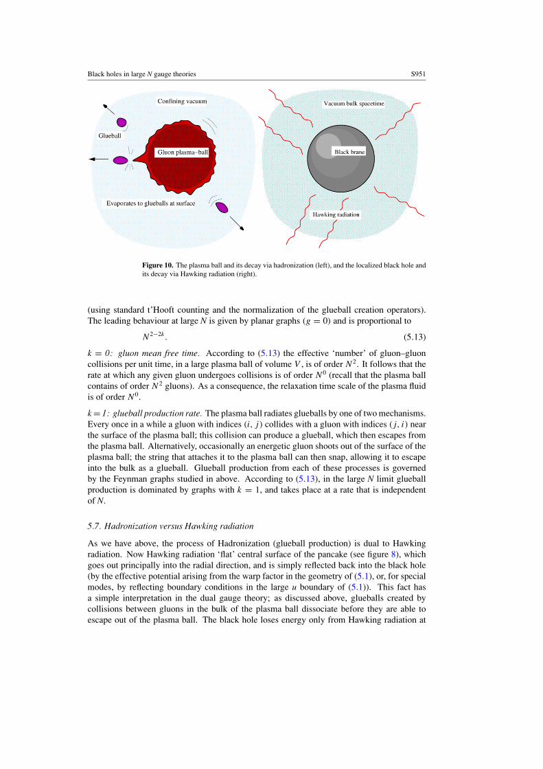
Figure 10. The plasma ball and its decay via hadronization (left), and the localized black hole andits decay via Hawking radiation (right).

(using standard t’Hooft counting and the normalization of the glueball creation operators).The leading behaviour at large N is given by planar graphs (g = 0) and is proportional to

N2−2k. (5.13)

k = 0: gluon mean free time. According to (5.13) the effective ‘number’ of gluon–gluoncollisions per unit time, in a large plasma ball of volume V , is of order N2. It follows that therate at which any given gluon undergoes collisions is of order N0 (recall that the plasma ballcontains of order N2 gluons). As a consequence, the relaxation time scale of the plasma fluidis of order N0.

k = 1: glueball production rate. The plasma ball radiates glueballs by one of two mechanisms.Every once in a while a gluon with indices (i, j) collides with a gluon with indices (j, i) nearthe surface of the plasma ball; this collision can produce a glueball, which then escapes fromthe plasma ball. Alternatively, occasionally an energetic gluon shoots out of the surface of theplasma ball; the string that attaches it to the plasma ball can then snap, allowing it to escapeinto the bulk as a glueball. Glueball production from each of these processes is governedby the Feynman graphs studied in above. According to (5.13), in the large N limit glueballproduction is dominated by graphs with k = 1, and takes place at a rate that is independentof N.

5.7. Hadronization versus Hawking radiation

As we have above, the process of Hadronization (glueball production) is dual to Hawkingradiation. Now Hawking radiation ‘flat’ central surface of the pancake (see figure 8), whichgoes out principally into the radial direction, and is simply reflected back into the black hole(by the effective potential arising from the warp factor in the geometry of (5.1), or, for specialmodes, by reflecting boundary conditions in the large u boundary of (5.1)). This fact hasa simple interpretation in the dual gauge theory; as discussed above, glueballs created bycollisions between gluons in the bulk of the plasma ball dissociate before they are able toescape out of the plasma ball. The black hole loses energy only from Hawking radiation at

S952 S Minwalla

its edge, reflecting the fact that only glueballs produced by gluon–gluon collisions near thesurface of the plasma ball can escape out into open space.

In this subsection we have focused on the radiation of glueballs from plasma balls.However the arguments of this section apply equally well to the time-reversed process.Consider a glueball incident upon the plasma ball from outside. Equation (5.13) impliesthat the interaction cross section for this glueball, per unit length traversed through the plasmaball, is of order N0. We expect this interaction process to lead to the glueballs dissolving intothe plasma ball. Similarly, glueballs formed in a gluon collision far from the surface of a largeplasma ball will dissolve before they escape, so the hadronization rate is proportional to thesurface area of the plasma ball rather than its volume.

5.8. Plasma-ball production in hadron–hadron collisions

Consider the collision of two stable glueballs (with masses of order �gap) at centre-of-massenergies large compared to N2�gap. In the large λ string theory dual these glueballs mapto light modes such as gravitons (or other light fields). Giddings [23] has emphasized that,at large λ, black hole production saturates the inclusive cross section for graviton collisionsat high enough energies (up to numbers of order unity); furthermore, this cross section alsosaturates the Froissart unitarity bound. We pause to review this argument. An upper boundfor the inclusive scattering cross section is easily estimated by assuming that gravitationalforces dominate at high enough energies. Then, the force between two colliding particlesseparated by impact parameter b may be estimated to be of order G4E

2

b2 e−�gapb, where wehave used the fact that gravity is massive in the relevant backgrounds. Consequently, incidentparticles simply sail past each other when b is larger than a number of order ln(E)/�gap (upto corrections that are subleading at large energies), and the inclusive cross section is boundedfrom above by

σ ∼ ln2(E)/�2

gap. (5.14)

However, one may independently use shock wave metrics and singularity theorems todemonstrate that the cross section for black hole formation is of the order of σ in (5.14)[23, 24].

As we have explained above, localized black holes map to localized lumps of gluonplasma in the dual field theory. It follows as a prediction of the AdS/CFT correspondencethat, at large N and large λ, two glueballs shot at each other (in the corresponding dual gaugetheory) with an impact parameter smaller than (ln(E)/�gap) will coalesce into a lump of gluonplasma with a probability close to one when E N2�gap. This lump of plasma, produced ata rate that saturates the Froissart bound, will typically settle into a very long lived plasma ball,which proceeds to slowly hadronize over a time scale of order N2, in the manner described inthe previous subsection. Note that even though the black hole forms with a size of order ln(E)

in the spatial directions of the field theory, it quickly expands to a size of order E1/p (whenthe dual field theory has p spatial dimensions) for which it can be meta-stable.

The reader may find the picture sketched in the last paragraph clashing with her QCD-trained intuition, which might lead her to expect the fast partonic constituents of the glueball toeither pass right through each other or to undergo a small number of hard collisions rather thansmoothly coalescing into a plasma ball. Of course the utility of partonic ideas is questionableat large λ (where partons interact strongly at all energies). Nevertheless, to the extent that thisnotion is valid, rapid gluon radiation ensures that the parton distribution function is peaked at

Black holes in large N gauge theories S953

small values of x [25] so that the average parton energy is of order

Eparton ≈ E

(�gap

E

)λ

(5.15)

where E is the centre-of-mass energy of the collision, ensuring that Eparton � �gap at large λ, sothat glueballs simply do not contain fast partons. Thus, at large N and large λ, glueball–glueballcollisions are conceptually similar to heavy ion collisions, with the large centre-of-mass energyshared between a large number of constituents.

At small λ, as mentioned above, most of the energy of the glueballs is carried by a smallnumber of partons, each of which carries a significant fraction (an energy of order E/ln(E))of the energy of the glueball (at high energies the partons tend to have smaller values of xdue to asymptotic freedom, but this is a logarithmic effect that does not affect our arguments).These very energetic partons interact weakly; their interactions will not form a plasma. As aconsequence we expect a crossover in the dominant behaviour of high energy scattering at λ

of order 1.18

It would be interesting (and may be possible) to quantitatively verify the qualitative picturesketched in this subsection.

6. Preliminary lessons for black holes from plasma balls

We will end these lectures with an extremely preliminary discussion of lessons for black holephysics that may be obtained from a study of plasma balls. This discussion will be short ofdetail, as very little work has yet been done along these lines.

6.1. Information conservation in Hawking radiation

It has often been pointed out that the AdS/CFT correspondence ensures that black holeevaporation is a unitary process. Our identification of specific gauge theory configurations(occurring in the decay process of plasma balls) with ‘small’ ten-dimensional Schwarzschildblack holes makes this argument more specific. The production of a plasma ball in a glueball–glueball collision, and its subsequent decay via hadronization is clearly a unitary process; theend point of this process is only approximately thermal.

Of course a full resolution of the information paradox requires the identification of the flawin Hawking’s argument that predicts a breakdown of unitarity. While the dual description ofHawking radiation is manifestly unitary, it has not yet proved possible to formulate Hawking’sargument in gauge theory language in order to identify its flaw. This is an important problemthat deserves attention.

6.2. How black is a black hole

It is a striking feature of classical black holes in general relativity (the feature responsible fortheir name) that a particle squarely incident on the black hole is always absorbed, no matterhow large its energy.

18 Note that even at small λ the glueball still contains a large number of small x partons whose strong interactionsmight create a lump of gluon plasma. However, this lump will not carry a finite fraction of the centre-of-mass collisionenergy. One might think that even if only a small plasma ball is formed, the fast partons would be bound to it bya string (since they carry a colour charge) so they would eventually be pulled back into it, given that strings cannotbreak in the large N limit. However, since in order to form the plasma we need an energy at least of order N2, the fastpartons will also carry an energy of order N2, allowing the relevant strings to snap even in the large N limit (sincetheir length would be of order N2).

S954 S Minwalla

In this paper we have identified a black hole with a plasma ball, a localized lump of gluonplasma at temperature Td . It might, at first, seem that a particle incident on the plasma ball atan energy E much larger than Td would sail right through it (undergoing a series of grazingcollisions that hardly affect it), in blatant contradiction with the expectations of black holephysics. We have already explained in subsection 6.2 that this naive expectation is incorrect.The only objects available to be hurled at the plasma ball are glueballs. At large λ glueballsmay be thought of as consisting of a very large number of low energy partons; the averageparton energy is Eparton in (5.15). Note that Epart � �gap even in the limit E → ∞. Asa consequence, glueballs may always be absorbed by plasma balls, no matter how high theincidence energy.

As we have explained in subsection 6.2, however, glueballs at small λ are composeddominantly of a small number of high energy partons. We expect that these partons shouldsimply blast through the plasma ball at high enough E (note that E may have to be of orderN in order to permit these partons to snap confining strings that may bind them to the plasmaball and to escape all the way to infinity, since the snapping probability per unit time and unitlength of the string is of order 1/N2). Thus, plasma balls at small λ (where string correctionsare very important) do not share all the properties of their large λ cousins (in particular theyno longer efficiently absorb glueballs).

7. Outlook for the future

We began these lectures expressing the conviction that dual gauge description of gravitationalsystems should prove useful in addressing long-standing puzzles in the theory of gravity. Thecomputations, constructions and ideas presented in these lectures only constitute a preliminarystep in this direction. In order to make further progress, it would be useful to formulate asharply defined gauge (and preferably ‘natural’) theory computation, whose result (no matterhow hard this would be to obtain in practice) would yield a clear answer to a gravitationalanswer. This has proven difficult to achieve so far, partly because our current understandingof the AdS/CFT dictionary does not permit an easy investigation of local bulk physics. It maywell turn out that, in order to make further progress we will be forced to better understandhow the strong coupling dynamics of Yang–Mills theory generates physics that is (at leastapproximately) local and (exactly) general coordinate invariant. We end these lectures withthis thought.

Appendix. The boundary stress tensor for compactifications of AdSd+2

Asymptotically AdSd+2 backgrounds possess a conserved (d + 1)-dimensional stress tensor[26–30]. The stress tensor associated with (5.1) is (see equations (4) and (25) in [31])

Tµν = �µν − γµν� − (d − 1)γµν = α e−(d−1)u

2(−δµν + (d + 1)δµθδνθ ), (A.1)

where the indices µ and ν run over i, t, θ, γµν is the restriction of (5.1) to a constant u slice,�µν = − 1

21√guu

dγµν

duand α = (d + 1)−(d+1). The boundary field theory stress tensor associated

with (5.1) is obtained by multiplying (A.1) by e(d−1)u, so that

T confined vacuumµν = α

2(−δµν + (d + 1)δµθδνθ ). (A.2)

The boundary stress tensor for the black brane solution (5.5) is obtained similarly, giving,

T black braneµν = (2πT )d+1 α

2(−δµν + (d + 1)δµt δνt ). (A.3)

Black holes in large N gauge theories S955

The subtraction we used to define the stress tensor in (A.1) is the standard subtractionfor the (d + 1)-dimensional field theory, which gives a vanishing stress tensor in the vacuumof this theory. From the point of view of the d-dimensional field theory which we obtainafter compactifying on the circle, it is more natural to use a different subtraction in which thestress tensor in the vacuum (5.1) of this theory evaluates to zero. Performing the necessarysubtraction we find

T black brane-subµν = α

2[−((2πT )d+1 − 1)δµν + (d + 1)((2πT )d+1δµtδνt − δµθδνθ )]. (A.4)

In particular, the energy density ε, free energy density f and pressure P of the black brane(the deconfined phase) are given as functions of temperature by

ε = α

2(d(2πT )d+1 + 1); P = −f = α

2((2πT )d+1 − 1). (A.5)

References

[1] Sundborg B 2000 The Hagedorn transition, deconfinement and N = 4 SYM theory Nucl. Phys. B 573 349(Preprint hep-th/9908001)

[2] Aharony O, Marsano J, Minwalla S, Papadodimas K and Van Raamsdonk M 2004 The Hagedorn/deconfinementphase transition in weakly coupled large N gauge theories Adv. Theor. Math. Phys. 8 603 (Preprinthep-th/0310285)

[3] Aharony O, Marsano J, Minwalla S, Papadodimas K and Van Raamsdonk M 2005 A first orderdeconfinement transition in large N Yang–mills theory on a small 3-sphere Phys. Rev. D 71 125018 (Preprinthep-th/0502149)

[4] Aharony O, Minwalla S and Wiseman T 2006 Plasma balls in large-N gauge theories and localized black holesClass. Quantum Grav. 23 2171 (Preprint hep-th/0507219)

[5] Hubeny V E and Rangamani M 2002 Unstable horizons J. High Energy Phys. JHEP05(2002)027 (Preprinthep-th/0202189)

[6] Aharony O, Gubser S S, Maldacena J M, Ooguri H and Oz Y 2000 Large N field theories, string theory andgravity Phys. Rep. 323 183 (Preprint hep-th/9905111)

[7] Barbon J L and Rabinovici E 2002 Closed-string tachyons and the Hagedorn transition in AdS space J. HighEnergy Phys. JHEP03(2002)057 (Preprint hep-th/0112173)

[8] Hawking S W and Page D N 1983 Thermodynamics of black holes in anti-de Sitter space Commun. Math.Phys. 87 577

[9] Witten E 1998 Anti-de Sitter space, thermal phase transition, and confinement in gauge theories Adv. Theor.Math. Phys. 2 505 (Preprint hep-th/9803131)

[10] Gross D J and Witten E 1980 Possible third order phase transition in the large N lattice gauge theory Phys. Rev.D 21 446

Wadia S A study of U(N) lattice gauge theory in two-dimensions Preprint EFI-79/44-CHICAGOWadia S R 1980 N = ∞ phase transition in a class of exactly soluble model lattice gauge theories Phys. Lett.

B 93 403[11] Goldschmidt Y Y 1980 1/N expansion in two-dimensional lattice gauge theory J. Math. Phys. 21 1842[12] Polchinski J 1992 High temperature limit of the confining phase Phys. Rev. Lett. 68 1267 (Preprint

hep-th/9109007)[13] Kutasov D 1994 Two-dimensional QCD coupled to adjoint matter and string theory Nucl. Phys. B 414 33

(Preprint hep-th/9306013)[14] Burgess C P, Constable N R and Myers R C 1999 The free energy of N = 4 Super Yang–Mills and the AdS/CFT

correspondence J. High Energy Phys. JHEP08(1999)017 (Preprint hep-th/9907188)[15] Kutasov D and Larsen F 2001 Partition sums and entropy bounds in weakly coupled CFT J. High Energy Phys.

JHEP01(2001)001 (Preprint hep-th/0009244)[16] Landsteiner K and Lopez E 1999 The thermodynamic potentials of Kerr–AdS black holes and their CFT duals

J. High Energy Phys. JHEP12(1999)020 (Preprint hep-th/9911124)[17] Pisarski R D and Tytgat M 1997 Why the SU(infinity) deconfining phase transition might be of second order

Preprint hep-ph/9702340[18] Alvarez-Gaume L, Gomez C, Liu H and Wadia S 2005 Finite temperature effective action, AdS(5) black holes,

and 1/N Phys. Rev. D 71 124023 (Preprint hep-th/0502227)

S956 S Minwalla

[19] Basu P and Wadia S R 2006 Phys. Rev. D 73 045022 (Preprint hep-th/0506203)[20] Alvarez-Gaume L, Basu P, Marino M and Wadia S R 2006 Blackhole/string transition for the small

Schwarzschild blackhole of AdS5 × S5 and critical unitary matrix models Preprint hep-th/0605041[21] Aharony O, Marsano J and Van Raamsdonk M 2006 Two loop partition function for large N pure Yang–Mills

theory on a small 3-sphere Preprint hep-th/0608156[22] Horowitz G T and Myers R C 1999 The AdS/CFT correspondence and a new positive energy conjecture for

general relativity Phys. Rev. D 59 026005 (Preprint hep-th/9808079)[23] Giddings S B 2003 High energy QCD scattering, the shape of gravity on an IR brane, and the Froissart bound

Phys. Rev. D 67 126001 (Preprint hep-th/0203004)Eardley D M and Giddings S B 2002 Phys. Rev. D 66 044011 (Preprint gr-qc/0201034)

[24] Kang K and Nastase H 2005 Phys. Lett. B 624 125 (Preprint hep-th/0501038)[25] Polchinski J and Strassler M J 2003 Deep inelastic scattering and gauge/string duality J. High Energy Phys.

JHEP05(2003)012 (Preprint hep-th/0209211)[26] Brown J D and York J W 1993 Quasilocal energy and conserved charges derived from the gravitational action

Phys. Rev. D 47 1407[27] Balasubramanian V and Kraus P 1999 Commun. Math. Phys. 208 413 (Preprint hep-th/9902121)[28] Henningson M and Skenderis K 2000 Fortsch. Phys. 48 125 (Preprint hep-th/9812032)[29] de Haro S, Solodukhin S N and Skenderis K 2001 Holographic reconstruction of spacetime and renormalization

in the AdS/CFT Commun. Math. Phys. 217 595 (Preprint hep-th/0002230)[30] Skenderis K 2001 Int. J. Mod. Phys. A 16 740 (Preprint hep-th/0010138)[31] Kraus P, Larsen F and Siebelink R 1999 The gravitational action in asymptotically AdS and flat spacetimes

Nucl. Phys. B 563 259 (Preprint hep-th/9906127)