Black-Box Obfuscation for d-CNFs

Zvika Brakerski Guy N. Rothblum

Abstract

We show how to securely obfuscate a new class of functions: conjunctions of NC0d circuits.These are functions of the form C(~x) =

∧mi=1 Ci(~x), where each Ci is a boolean NC0d circuit,

whose output bit is only a function of d = O(1) bits of the input ~x. For example, d-CNFs,where each clause is a disjunction of at most d variables, are in this class. Given such a function,we produce an obfuscated program that preserves the input-output functionality of the givenfunction, but reveals nothing else. Our construction is based on multilinear maps, and can beinstantiated using the recent candidates proposed by Garg, Gentry and Halevi (EUROCRYPT2013) and by Coron, Lepoint and Tibouchi (CRYPTO 2013).

We prove that the construction is a secure obfuscation in a generic multilinear group model,under the black-box definition of Barak et al. (CRYPTO 2001). Security is based on a new worst-case hardness assumption about exponential hardness of the NP-complete problem 3-SAT, theBounded Speedup Hypothesis.

One of the new techniques we introduce is a method for enforcing input consistency, whichwe call randomizing sub-assignments. We hope that this technique can find further applicationin constructing secure obfuscators.

The family of functions we obfuscate is considerably richer than previous works that considerblack-box obfuscation.1 As one application, we show how to achieve obfuscated functional pointtesting: namely, to construct a circuit that checks whether f(~x) = ~y, where f is an arbitrary“public” polynomial-time computable function, but ~y is a “secret” point that is hidden in theobfuscation.

1 Introduction

A code obfuscator is a compiler that makes computer programs impossible to reverse engineer, whilepreserving their input-output functionality. Code obfuscation is a central question in the theoryand practice of cryptography. Despite the problem’s importance, very few techniques or heuristicswere known. Recently, however, several works have leveraged new constructions of cryptographi-cally secure multilinear maps [GGH12, CLT13] to construct obfuscators for complex functionalities[BR13, GGH+13].

In this work, we present a candidate obfuscator for a rich new circuit class: conjunctions ofNC0 circuits. In particular, this includes the family of d-CNF formulas (for constant d). Our con-struction relies on (asymmetric) multilinear maps, and can be instantiated using the new candidateconstructions of Garg, Gentry and Halevi [GGH12], or of Coron, Lepoint and Tibouchi [CLT13].

We prove the construction’s security in a generic multilinear map model, under a worst-casecomplexity assumption (see below). An important ingredient in this construction, which we hope

1A concurrent and independent work of Garg et al. [GGH+13] considers the weaker security notion of “indis-tinguishability obfuscation”, and proposes a candidate obfuscator for any function computed by a polynomial sizecircuit.

1

will find further applications, is a new technique for enforcing input consistency using randomizingsub-assignments.

Obfuscation: Definitions. Intuitively, an obfuscator should generate a new program that pre-serves the the original program’s functionality, but is impossible to reverse engineer. The theoreticalstudy of this problem was initiated by Barak et al. [BGI+12]. They formalized a strong simulation-based security requirement of black box obfuscation: namely, the obfuscated program should exposenothing more than what can be learned via oracle access to its input-output behavior. We refer tothis notion as “black-box” obfuscation, and we use this strong formalization throughout this work(except where we note otherwise).

A weaker notion of obfuscation, known as indistinguishability or best-possible obfuscation wasstudied in [BGI+12, GR07]. An indistinguishability obfuscator guarantees that the obfuscations ofany two programs (boolean circuits) with identical functionalities are indistinguishable. We notethat, unlike the black-box definition of security, indistinguishability obfuscation does not quantifyor qualify what information the obfuscation might expose. In particular, the obfuscation mightreveal non-black-box information about the functionality.

Prior Work: Negative Results. In their work, [BGI+12] proved the impossibility of general-purpose black-box obfuscators (i.e. ones that work for any polynomial-time functionality) in thevirtual black box model. This impossibility result was extended in [GK05]. While these negativeresults show serious limitations on the possibility of general-purpose obfuscation, they focus onspecific (often cryptographic or contrived) functionalities. Thus, they do not rule out that obfus-cation may be possible for many programs of interest. Goldwasser and Rothblum [GR07] showedobstacles to the possibility of achieving indistinguishability obfuscation with information-theoreticsecurity, and to achieving it in the random oracle model.

Prior Work: Positive Results. Positive results on obfuscation focused on specific, simple pro-grams. One program family, which has received extensive attention, is that of “point functions”:password checking programs that only accept a single input string, and reject all others. Startingwith the work of Canetti [Can97], several works have shown obfuscators for this family under vari-ous assumptions [CMR98, LPS04, Wee05], as well as extensions [CD08, BC10]. Canetti, Rothblumand Varia [CRV10] showed how to obfuscate a function that checks membership in a hyperplane ofconstant dimension (over a large finite field). Other works showed how to obfuscate cryptographicfunction classes under different definitions and formalizations. These function classes include check-ing proximity to a hidden point [DS05], vote mixing [AW07], and re-encryption [HRSV11]. Severalworks [Can97, CMR98, HMLS10, HRSV11] relaxed the security requirement so that obfuscationonly holds for a random choice of a program from the family.

More recently, Brakerski and Rothblum [BR13] showed that multilinear maps could be used toobfuscate richer function families. They constructed an obfuscator for conjunctions, the family offunctions that test whether a subset of the input bits take on specified values. The constructionwas shown to be secure in the generic multilinear map model. It was also shown to be secure under(falsifiable [Nao03]) multilinear DDH-like assumptions, so long as the conjunction is drawn from afamily with sufficient entropy.

2

Related Concurrent Work [GGH+13]. In a concurrent and independent work, Garg etal. [GGH+13] use cryptographic multilinear maps to give a candidate indistinguishability obfuscator(see above) for all polynomial-size circuits. The main differences with our work are: (i) we constructan obfuscator with the stronger security notion of black-box obfuscation (albeit for a smaller classof functions). And (ii) we prove the security of our construction in the generic multilinear groupmodel. See more on the generic multilinear group model below. Our proof uses a worst-casecomplexity-theoretic assumption. Garg et al. [GGH+13] pose the security of their construction inthe generic multilinear group model as a major open question. We note that [GGH+13] do provesecurity in a new “generic colored matrix model”, which restricts an adversary to a subset of themultilinear group operations.

Our Work: Black-Box Obfuscation for Conjunctions of NC0. An NC0d circuit is a boolean

circuit on n-bit inputs, whose output depends only on d input bits. If a circuit (or rather a circuitensemble) is in NC0

d for some fixed d ≥ 0, then we say that it is in NC0 (and we drop the d). Aconjunction of NC0 circuits is a circuit C =

∧mi=1Ci, where each Ci is an NC0 circuit. We use

CNC0 to refer to the class of circuits that are conjunctions of NC0 circuits. For example, any d-CNF(a CNF formula, where each clause has at most d literals) is a CNC0 circuit. Another example issimple conjunction circuits: there each Ci only depends on (at most) a single input bit.

In this work we build a black-box obfuscator for CNC0 circuits. In more detail, the obfuscatortakes as input a CNC0

d circuit C, runs in time O(nd), and outputs and obfuscation that exposesnothing beyond the input-output functionality of C (the obfuscation also exposes d). We note thatthe class CNC0 is limited in computational power. In particular, it is contained in AC0, and sothere are simple and natural functions (such as XOR) that cannot be computed in CNC0. Still,it is significantly richer than previous classes for which obfuscators were known. For example,the Cook-Levin Theorem shows that NP-complete statements can be verified in CNC0, and thereare secure digital signature schemes where verification is in CNC0. Moreover, impossibility results[BGI+12, GK05] rule out general-purpose black-box obfuscation even for AC0. Obfuscating CNC0

brings us close to the dovetailing with these impossibility results.One important ingredient in this construction is a new technique for enforcing input consistency

by randomizing sub-assignments. We are hopeful that this technique may find further applications.We prove that the construction is a secure black-box obfuscator in the generic multilinear

group model. In the generic multilinear group model, an adversary must operate independently ofgroup elements’ representations. Rather, the adversary is given arbitrary strings representing theseelements, and can only manipulate them using oracles for addition, subtraction, multilinear mapsand more (see below). In our proof, we make use of a new worst-case assumption about exponentialhardness of the NP-complete problem 3-SAT. We call this new assumption the bounded speeduphypothesis, a strengthening of the long-standing exponential time hypothesis (ETH) for solvingSAT [IP99].2 See further details below.

We find this proof of security intriguing for several reasons. First, as stated above, it tells usthat (under the bounded-speedup hypothesis) the construction is completely impervious to genericattacks—a rich class that of attacks, which in particular includes all known attacks against thecandidate cryptographic multilinear groups. While we distrust the generic model (especially inlight of impossibility results [BGI+12, GK05]), results in this model can still be used to obfuscate

2We note that is both the adversary and the simulator are allowed to run in quasi-polynomial tim, security canbe based on the (standard) Exponential-Time Hypothesis.

3

provided we have simple secure hardware implementing the generic group. Finally, to the bestof our knowledge, no impossibility results for black-box obfuscation are known in generic models(or in the random oracle model). This raises the possibility that our techniques could be used toconstruct a secure black-box obfuscator for richer classes, and even for any polynomial-size circuit,in the generic multilinear group model.

An Application: Obfuscated Functional Point Tests. Consider the following setting: thereis an arbitrary polynomial-size “public” circuit computing a function f , and a “secret” target value~y. We want to release an obfuscation that can test, for any input ~x, whether f(~x) = ~y, but withoutrevealing anything about the secret ~y. For example, perhaps C checks that its input contains amessage m, and a digital signature on m from a trusted authority (otherwise C rejects). If this testpasses, C runs a sophisticated analysis to determine m’s topic, and flags whether m’s topic equalsy. An adversary that receives the obfuscation (and knows the topic analysis algorithm) should notbe able to determine what the “target topic” y is—it can only test messages that have been signedby the trusted authority, and see whether their topic is y.

A obfuscator for CNC0 can be used for this application as follows. By the Cook-Levin theorem,for any polynomial-size C, there exists a CNC0

3 circuit C ′ that takes as input (~x,C(~x), w), wherew is “advice” computed as a function of C and of ~x only, and accept if and only if C(~x) = y.By obfuscating C ′ gives the desired application. We note that this type of application, involvinggeneral computations, is well beyond what was known to be possible for black-box obfuscation.

We proceed with further details and discussions.

1.1 Our Construction and its Security

Background on Multilinear Maps and Graded Encoding Schemes. We begin by recallingthe notion of multilinear maps, due to Boneh and Silverberg [BS02]. Rothblum [Rot13] consideredthe asymmetric case, where the groups may be different (this is crucial for our construction).

Definition 1.1 (Asymmetric Multilinear Map [BS02, Rot13]). For τ + 1 cyclic groups G1, . . . , Gτ ,GT of the same order p, a τ -multilinear map e : G1 × . . .×Gτ → G has the following properties:

1. For elements gi ∈ Gii=1,...,τ , index i ∈ [τ ] and integer α ∈ Zp, it holds that:

e(g1, . . . , α · gi, . . . , gτ ) = α · e(g1, . . . , gτ )

2. The map e is non-degenerate: when its inputs are all generators of their respective groupsGi, then its output is a generator of the group G.

Recently, [GGH12] suggested a candidate for graded encoding, a generalization of (symmetricor asymmetric) multilinear maps. See Section 2.1 for a more complete overview on these. For thisintroduction, we treat them as a generalization of asymmetric multilinear maps in the followingway. For the i-th group Gi, of prime order p, we consider the ring Zp. For an element σ ∈ Zp,we can think of gσi as an “encoding” of σ in Gi. We denote this by enci(σ). We note that thisencoding is easy to compute, but (presumably) hard to invert. The multilinear map e lets ustake τ encodings enci(σi)i∈[τ ],σi∈Zp

, and compute an encoding encT (∏i σi) in the “final group”

G. Graded encoding schemes provide a similar functionality, albeit with randomized and noisyencodings, and with a procedure for testing equality of encoded elements in the final group G.

4

Obfuscating Conjunctions of Bit-Predicates [BR13]. Recently, [BR13] show how to obfus-cate conjunction functions: conjunctions of single-bit predicates. A conjunction C(~x) =

∧i∈[n]Ci(~x[i])

is made up of a single circuit Ci for each input bit ~x[i]. The circuit Ci can equal ~x[i], its negation, orbe a constant 1 (meaning it has no effect) or 0 (meaning that C ≡ 0). For each i ∈ [n], the [BR13]obfuscator chooses an “accepting” ring element αi,0 and a “rejecting” ring element αi,1. It thenencodes the circuit Ci using a two-entry table, where each entry v ∈ 0, 1 contains the encodingsof a pair of ring elements:

(ρi,v, (ρi,v) · αi,Ci(v)))

(the ρi,v value is uniformly random). We emphasize that the obfuscation only produces the encod-ings of these ring elements. Note that e.g. if Ci ≡ 1, then both of these table entries use the sameα variable, and are thus not independent. Nonetheless, since the encodings are hard to invert, anadversary will not be able to tell that this is the case (which is essential for security).

To complete the obfuscation, the obfuscator also produces encodings of an “unlocking” or“checking” pair:

(ρchk, (ρchk · (∏i∈[n]

αi,1)))

(where again ρ is uniformly random, and chk is just a notation for the last group, n + 1 in thiscase).

To evaluate the obfuscated program on an input ~x ∈ 0, 1n, they use the multilinear map totest the equality:3ρchk · (∏

i∈[n]

(ρi,~x[i]) · αi,Ci(~x[i]))

?=

(ρchk · (∏i∈[n]

αi,1)) · (∏i∈[n]

ρi,~x[i])

(1)

Correctness follows by construction: the equality holds if and only if ∀i ∈ [n] : Ci(~x[i]) = 1 (exceptfor a negligible error probability).

Security is not as straightforward. Intuitively, security holds because for each i ∈ [n], theentries of the i-th table do not reveal anything about Ci (the complication is that the “checking”pair creates correlations between the different table entries. See [BR13]).

Our Contribution: Obfuscating Conjunctions of Multi-Bit Predicates. Our goal is ob-fuscating a CNC0 circuit C, where C is a conjunction of NC0 predicates C1, . . . , Cm. A naturalinitial approach is starting with the construction of [BR13], which obfuscates conjunctions of single-bit predicates, and trying to extend that construction to conjunctions of predicates on many (d)bits as follows. We can “group” every d-tuple of inputs bits into a “super-symbol”. This stretchesthe n-bit input into a vector of

(nd

)“super-symbols” in 0, 1d. Now, any predicate on d bits be-

comes a predicate on a single “super-symbol”, and we might hope to directly apply the conjunctionobfuscator.

There are two issues with this approach:

1. Each input “super-symbol” is now in 0, 1d (rather than 0, 1)3For the candidate of [GGH12], the encodings are randomized, but there is a procedure for testing equality between

encoded elements in the final group.

5

Examine one such super-symbol I, corresponding to a d-tuple of input bits (i.e. I is a set

of d elements out of [n], which we denote I ∈([n]d

)). Let CI be the circuit in C that takes

the d bits in I as its input bits.4 Of the 2d assignments to the bits in I, there is a subsetS1 ⊆ 0, 1d that makes CI accept. The remaining assignments S0 ⊆ 0, 1d, make CI reject.

Building on the conjunction obfuscator, we can now have a table of size 2d for the circuit CI ,where each table entry corresponds to an assignment for the variables in I. We choose an“accepting ring element” αI,1 and a “rejecting group element” αI,0. In each entry ~s ∈ 0, 1dwe encode either an “accepting pair” (ρI,~s, (ρI,~s ·αI,1)), or a “rejecting pair” (ρI,~s, (ρI,~s ·αI,0)).Intuitively, hardness of discreet log problems guarantees that an adversary cannot use thesetable to distinguish whether or not any given assignment satisfies the I-th sub-circuit.

Finally, to complete the obfuscation, we also include a “checking pair” that encodes a productof all the accepting group elements (ρchk, (ρchk ·

∏I∈([n]

d ) αI,1)).

To evaluate the obfuscated program on an input ~x ∈ 0, 1n, use the multilinear map, as inthe conjunction obfuscator, to test the equality:ρchk · ( ∏

I∈([n]d )

(ρI,~x|I · αI,~x|I ))

?=

ρchk · ( ∏I∈([n]

d )

αI,1) · (∏

I∈([n]d )

ρI,~x|I )

By construction, equality will hold if and only if ~x is an accepting input (except for a negligibleerror probability). The size of the resulting obfuscation is O(nd · 2d).

2. Enforcing Consistency

A more serious issue with the idea above, is enforcing consistency. Namely, there is nothing tostop an adversary from picking

(nd

)arbitrary assignments ~sI ∈ 0, 1dI∈([n]

d ), and evaluating

the “checking equality”:ρchk · ( ∏I∈([n]

d )

(ρI,~sI · αI,~sI ))

?=

ρchk · ( ∏I∈([n]

d )

αI,1) · (∏

I∈([n]d )

ρI,~sI )

We emphasize that the assignments ~sI might not be consistent: they need not correspond toany input ~x ∈ 0, 1n. For example, the first bit of ~x might be set to 0 in one set I, and to 1in another set I ′! Allowing an adversary to test such equalities would immediately leak nonblack-box information about the circuit C and would break security.

The main technical challenge in our construction is disallowing such attacks, and enforcingconsistency in the adversary’s choices. We view this as one of our main contributions, andwe hope that it can find further applications as a building-block for constructing secureobfuscators.

4We assume w.l.o.g. that there is a single such circuit CI in C: if there is none, then CI is the constant-1 circuits.If there are multiple such circuits, they can be merged into their conjunction, which is itself an NC0d circuit. Bothtransformations maintain the functionality of C and also maintain |C| ≤ O(n)d.

6

Randomizing Sub-Assignments and Enforcing Consistency. We want to avoid lettingan adversary choose inconsistent sub-assignments for the circuits CII∈([n]

d ). In particular, if

i ∈ I, I ′, then we want to ensure that the adversary can only pick sub-assignments ~sI , ~sI′ where~sI [i] = ~sI′ [i] ∈ 0, 1. Towards this end, we randomize each sub-assignment’s table entry as follows.

For each i ∈ [n] and I 3 i (we use I 3 i to denote I ∈([n]d

): i ∈ I), and for each bit value

b ∈ 0, 1, choose a uniformly random randomizer βI,i,b, and multiply it into each entry ~s ∈ 0, 1dof the table for I, so that entry now has encodings of:

(ρI,~s, (ρI,~s · αI,CI(~s) · (∏i∈I

βI,i,~s[i])))

Now in evaluating the “checking equality”, on the left-hand side we have a product of all theseβ-randomizers, i.e. we get an additional multiplicative term:∏

I∈([n]d ),i∈I

βI,i,~sI [i] =∏i∈[n]

(∏I3i

βI,i,~sI [i])

We pick the β-randomizers under the additional restriction that ∀i ∈ [n]:

(∏I3i

βI,i,0) = (∏I3i

βI,i,1) = γi

Otherwise the β variables are uniformly random. This has the effect that as long as the adversarypicks the sub-assignments involving variable i consistently, the new multiplicative term is exactly γi,regardless of whether the bit value assigned to the i-th input bit is 0 or 1. However, if assignmentsinvolving input bit i get inconsistent values, then the added multiplicative term will be differentfrom γi (indeed, it will be close to uniformly random and independent of γi).

We use the above randomization to enforce consistency. To allow functionality, we multiply thenew terms into the “checking pair”, which now has encodings of:

(ρchk, (ρchk ·∏

I∈([n]d )

αI,1 ·∏i∈[n]

γi))

The obfuscated program can now be evaluated using the target equation similarly to the above(with the added β terms enforcing consistency). Functionality follows by construction. Security isnot so straightforward: while the randomized sub-assignments do intuitively seem to aid in avoidinginconsistent assignments to the sub-circuits, proving that the construction is secure seems to beconsiderably more difficult.

Security in the Generic Model and the Bounded-Speedup Hypothesis We prove thatour construction is a secure black-box obfuscator in the generic multilinear group model. In thisproof, we make use of a new worst-case assumption about exponential hardness of the NP-completeproblem 3-SAT. We call this new assumption the bounded speedup hypothesis, a strengthening ofthe long-standing exponential time hypothesis for solving SAT [IP99]. The exponential-time hy-pothesis states that no sub-exponential time algorithm can resolve satisfiability of 3-CNF formulas.Intuitively, the bounded-speedup hypothesis states that no polynomial-time algorithm for resolv-ing satisfiability of 3-CNFs can have “super-polynomial speedup” over a brute-force algorithm that

7

tests assignments one-by-one. More formally, there does not exist an ensemble of polynomial-sizecircuits An, and an ensemble of super-polynomial-size sets of assignments Xn, such that oninput a 3-CNF Φ on n-bit inputs, w.h.p. An finds a satisfying assignment for Φ in Xn if such anassignment exists. We emphasize that this is a worst-case hypothesis, i.e. it only says that for everyensemble A, there exists some 3-CNF on which A fails. See Definition 5.3, and further discussionin Appendix A below.

At an intuitive (and somewhat inaccurate) level, the security proof uses the randomizing sub-assignments to argue that the only “interesting” computations that an adversary can run in thegeneric model are: (i) evaluate the “checking equation” on a consistently chosen input ~x, or (ii)evaluate a linear combination of the checking equations for a set X of inputs. For any othercomputations that the adversary runs, the answer is essentially independent of the obfuscatedcircuit C, and can be simulated.

For computations that evaluate a linear combination of the checking equation for inputs in a setX , the answer can be simulated using only black-box access to C on those inputs. The remainingchallenge is to argue that the adversary can only evaluate a linear combination of polynomially manyinputs, i.e. that the set X must be of polynomial size. To show this, we prove that an adversarythat computes a linear combination of the checking equation for a set of inputs X , can also resolve3-SAT on this same set X : given any 3-CNF Φ, it can find a satisfying assignment for Φ in X (ifone exists). Thus, under the Bounded Speedup Hypothesis, the set X must be of polynomial size,and the adversary can be simulated. We note that one detail (among many) omitted above, is howthe simulator can “extract” the set X to complete the simulation. See details in Section 5.

2 Preliminaries

For all n, d ∈ N we define([n]d

)to be the set of lexicographically ordered sets of cardinality d in [n].

More formally: ([n]

d

)=〈i1, . . . , id〉 ∈ [n]d : i1 < · · · < id

.

Note that∣∣∣([n]

d

)∣∣∣ =(nd

).

For ~x ∈ 0, 1n and I = 〈i1, . . . , id〉 ∈([n]d

), we let ~x|I ∈ 0, 1d denote the vector 〈~x[i1], . . . , ~x[id]〉.

We often slightly abuse notation when working with ~s = ~x|I , and let ~s[ij ] denote the element x[ij ]

(rather than the ijth element in ~s). We sometimes overload notation and use I ∈([n]d

)to denote

the lexicographic ordinal of I in([n]d

)(which is an integer in

[(nd

)]). We use I 3 i to denote the set

of sets I ∈([n]d

): i ∈ I. Namely, all the sets in

([n]d

)which contain the element i.

2.1 Graded Encoding Schemes

We begin with the definition of a graded encoding scheme, due to Garg, Gentry and Halevi [GGH12].While their construction is very general, for our purposes a more restricted setting is sufficient asdefined below.

Definition 2.1 (τ -Graded Encoding Scheme [GGH12]). A τ -encoding scheme for an integer τ ∈ Nand ring R, is a collection of sets S = S(α)

~v ⊂ 0, 1∗ : ~v ∈ 0, 1τ , α ∈ R with the followingproperties:

8

1. For every index ~v ∈ 0, 1τ , the sets S(α)~v : α ∈ R are disjoint, and so they are a partition

of the indexed set S~v =⋃α∈R S

(α)~v .

2. There are binary operations “+” and “−” such that for all ~v ∈ 0, 1τ , α1, α2 ∈ R and for all

u1 ∈ S(α1)~v , u2 ∈ S(α2)

~v :

u1 + u2 ∈ S(α1+α2)~v and u1 − u2 ∈ S(α1−α2)

~v ,

where α1 + α2 and α1 − α2 are addition and subtraction in R.

3. There is an associative binary operation “×” such that for all ~v1, ~v2 ∈ 0, 1τ such that

~v1 + ~v2 ∈ 0, 1τ , for all α1, α2 ∈ R and for all u1 ∈ S(α1)~v1

, u2 ∈ S(α2)~v2

, it holds that

u1 × u2 ∈ S(α1·α2)~v1+~v2

,

where α1 · α2 is multiplication in R.

In this work, the ring R will always be Zp for a prime p.

For the reader who is familiar with [GGH12], we note that the above is the special case oftheir construction, in which we consider only binary index vectors (in the [GGH12] notation, thiscorresponds to setting κ = 1), and we construct our encoding schemes to be asymmetric (as willbecome apparent below when we define our zero-text index vzt = ~1).

Definition 2.2 (Efficient Procedures for a τ -Graded Encoding Scheme [GGH12]). We considerτ -graded encoding schemes (see above) where the following procedures are efficiently computable.

• Instance Generation: InstGen(1λ, 1τ ) outputs the set of parameters params, a description ofa τ -Graded Encoding Scheme. (Recall that we only consider Graded Encoding Schemes overthe set indices 0, 1τ , with zero testing in the set S~1). In addition, the procedure outputsa subset evparams ⊂ params that is sufficient for computing addition, multiplication andzero testing5 (but possibly insufficient for encoding or for randomization).

• Ring Sampler: samp(params) outputs a “level zero encoding” a ∈ S(α)0 for a nearly uniform

α ∈R R.

• Encode and Re-Randomize:6 encRand(params, i, a) takes as input an index i ∈ τ and a ∈S

(α)0 , and outputs an encoding u ∈ S(α)

~ei, where the distribution of u is (statistically close to

being) only dependent on α and not otherwise dependent of a.

• Addition and Negation: add(evparams, u1, u2) takes u1 ∈ S(α1)~v , u2 ∈ S

(α2)~v , and outputs

w ∈ S(α1+α2)~v . (If the two operands are not in the same indexed set, then add returns ⊥).

We often use the notation u1 + u2 to denote this operation when evparams is clear from the

context. Similarly, negate(evparams, u1) ∈ S(−α1)~v .

5The “zero testing” parameter pzt defined in [GGH12] is a part of evparams.6This functionality is not explicitly provided by [GGH12], however it can be obtained by combining their encoding

and re-randomization procedures.

9

• Multiplication: mult(evparams, u1, u2) takes u1 ∈ S(α1)~v1

, u2 ∈ S(α2)~v2

. If ~v1 + ~v2 ∈ 0, 1τ (i.e.

every coordinate in ~v1 + ~v2 is at most 1), then mult outputs w ∈ S(α1·α2)~v1+~v2

. Otherwise, multoutputs ⊥. We often use the notation u1 × u2 to denote this operation when evparams isclear from the context.

• Zero Test: isZero(evparams, u) outputs 1 if u ∈ S(0)~1

, and 0 otherwise.

In the [GGH12, CLT13] constructions, encodings are noisy and the noise level increases withaddition and multiplication operations, so one has to be careful not to go over a specified noisebound. However, the parameters can be set so as to support O(τ) operations, which are sufficient forour purposes. We therefore ignore noise management throughout this manuscript. An additionalsubtle issue is that with negligible probability the initial noise may be too big. However this canbe avoided by adding rejection sampling to samp and therefore ignored throughout the manuscriptas well.

As was done in [BR13], our definition deviates from that of [GGH12]. We define two sets ofparameters params and evparams. While the former will be used by the obfuscator in our con-struction (and therefore will not be revealed to an external adversary), the latter will be used whenevaluating an obfuscated program (and thus will be known to an adversary). When instantiatingour definition, the guideline is to make evparams minimal so as to give the least amount of infor-mation to the adversary. In particular, in the known candidates [GGH12, CLT13], evparams onlyneeds to contain the zero-test parameter pzt (as well as the global modulus).

2.2 Obfuscation

Definition 2.3 (Virtual Black-Box Obfuscator [BGI+12]). Let C = Cnn∈N be a family ofpolynomial-size circuits, where Cn is a set of boolean circuits operating on inputs of length n.And let O be a PPTM algorithm, which takes as input an input length n ∈ N, a circuit C ∈ Cn, asecurity parameter λ ∈ N, and outputs a boolean circuit O(C) (not necessarily in C).O is an obfuscator for the circuit family C if it satisfies:

1. Preserving Functionality: For every n ∈ N, and every C ∈ Cn, and every ~x ∈ 0, 1n, with allbut negl(λ) probability over the coins of O:

(O(C, 1n, λ))(~x) = C(~x)

2. Polynomial Slowdown: For every n, λ ∈ N and C ∈ C, the circuit O(C, 1n, 1λ) is of size atmost poly(|C|, n, λ).

3. Virtual Black-Box: For every (non-uniform) polynomial size adversary A, there exists a (non-uniform) polynomial size simulator S, such that for every n ∈ N and for every C ∈ Cn:∣∣ Pr

O,A[A(O(C, 1n, 1λ)) = 1]− Pr

S[SC(1|C|, 1n, 1λ) = 1]

∣∣ = negl(λ)

Remark 2.4. A stronger notion of functionality, which also appears in the literature, requires thatwith overwhelming probability the obfuscated circuit is correct on every input simultaneously. Weuse the relaxed requirement that for every input (individually) the obfuscated circuit is correct withoverwhelming probability (in both cases the probability is only over the obfuscator’s coins). We notethat our construction can be modified to achieve the stronger functionality property (by using a ringof sufficiently large size and the union bound).

10

3 The Generic Graded Encoding Scheme Model

We would like to prove the security of our construction against generic adversaries. To this end,we will use the generic graded encoding scheme model, which was previously used in [BR13], and isanalogous to the generic group model (see Shoup [Sho97] and Maurer [Mau05]). In this model, analgorithm/adversary A can only interact with the graded encoding scheme via oracle calls to theadd, mult, and isZero operations from Definition 2.2. Note that, in particular, we only allow accessto the operations that can be run using evparams. To the best of our knowledge, non-genericattacks on known schemes, e.g. [GGH12], require use of params and cannot be mounted whenonly evparams is given.

We use G to denote an oracle that answers adversary calls. The oracle operates as follows:

for each index ~v ∈ 0, 1τ , the elements of the indexed set S~v =⋃α∈R S

(α)~v are arbitrary binary

strings. The adversary A can manipulate these strings using oracle calls (via G) to the gradedencoding scheme’s functionalities. For example, the adversary can use G to perform an add call:

taking strings s1 ∈ S(α1)~v , s2 ∈ S(α2)

~v , encoding indexed ring elements (~v, α1), (~v, α2) (respectively),

and obtaining a string s ∈ S(α1+α2)~v , encoding the indexed ring element (~v, (α1 + α2)).

We say that A is a generic algorithm (or adversary) for a problem on graded encoding schemes(e.g. for computing a moral equivalent of discreet log), if it can accomplish this task with respectto any oracle representing a graded encoding scheme, see below.

In the add example above, there may be many strings/encodings in the set S(α1+α2)~v . One

immediate question is which of these elements should be returned by the call to add. In ourabstraction, for each ~v ∈ 0, 1τ and α ∈ R, G always uses a single unique encoding of the indexedring element (~v, α). I.e. the set Sα~v is a singleton. Thus, the representation of items in the gradedencoding scheme is given by a map σ(~v, α) from ~v ∈ 0, 1τ and α ∈ R, to 0, 1∗. We restrict ourattention to the case where this mapping has polynomial blowup.

Remark 3.1 (Unique versus Randomized Representation). We note that the known candidates ofsecure graded encoding schemes [GGH12, CLT13] do not provide unique encodings: their encodingsare probabilistic. Nonetheless, in the generic graded encoding scheme abstraction we find it helpful torestrict our attention to schemes with unique encodings. For the purposes of proving security againstgeneric adversaries, this makes sense: a generic adversary should work for any implementation ofthe oracle G, and in particular also for an implementation that uses unique encodings.

Moreover, our perspective is that unique encodings are more “helpful” to an adversary than ran-domized encodings: a unique encoding gives the adversary the additional power to “automatically”check whether two encodings are of the same indexed ring element (without consulting the oracle).Thus, we prefer to prove security against generic adversaries even for unique representations.

It is important to note that the set of legal encodings may be very sparse within the set ofimages of σ, and indeed this is the main setting we will consider when we study the generic model.In this case, the only way for A to obtain a valid representation of any element in any graded setis via calls to the oracle (except with negligible probability). Finally, we note that if oracle callscontain invalid operators (e.g. the input is not an encoding of an element in any graded set, theinputs to add are not in the same graded set, etc.), then the oracle returns ⊥.

Random Graded Encoding Scheme Oracle. We focus on a particular randomized oracle:the random generic encoding scheme (GES) oracle RG. RG operates as follows: for each indexed

11

ring element (with index ~v ∈ 0, 1τ and ring element σ ∈ R), its encoding is of length ` =(|τ | · log |R| ·poly(λ)) (where |τ | is the bit representation length of τ). The encoding of each indexedring element is a uniformly random string of length `. In particular, this implies that the only waythat A can obtain valid encodings is by calls to the oracle RG (except with negligible probability).

The definition of secure obfuscation in the random GES model is as follows.

Definition 3.2 (Virtual Black-Box in the Random GES Model). Let C = Cnn∈N be a family ofcircuits and O a PPTM as in Definition 2.3.

A generic algorithm ORG is an obfuscator in the random generic encoding scheme model, if itsatisfies the functionality and polynomial slowdown properties of Definition 2.3 with respect to Cand to any GES oracle RG, but the virtual black-box property is replaced with:

3. Virtual Black-Box in the Random GES Model: For every (non-uniform) polynomial sizegeneric adversary A, there exists a (non-uniform) generic polynomial size simulator S, suchthat for every n ∈ N and every C ∈ Cn:∣∣( Pr

RG,O,A[ARG(ORG(C, 1n, 1λ))] = 1)− ( Pr

RG,S[SC(1|C|, 1n, 1λ)] = 1)

∣∣ = negl(λ)

We remark that while it makes sense to allow S to access the oracle RG, this is in fact notnecessary. This is since RG can be implemented in polynomial time (as described below), andtherefore S can just implement it by itself.

Online Random GES Oracle. In our proof, we will use the property that the oracle RG can beapproximated to within negligible statistical distance by an online polynomial time process, whichsamples the representations on-the-fly. Specifically, the oracle will maintain a table of entries of

the form (~v, α, label~v,α), where label~v,α ∈ 0, 1` is the representation of S(α)~v in RG (the table is

initially empty). Every time RG is called for some functionality, it checks that its operands indeedcorrespond to an entry in the table, in which case it can retrieve the appropriate (~v, α) to performthe operation (if the operands are not in the table, RG returns ⊥). Whenever RG needs to return a

value S(α)~v , it checks whether (~v, α) is already in the table, and if so returns the appropriate label~v,α.

Otherwise it samples a new uniform label, and inserts a new entry into the table.When interacting with an adversary that only makes a polynomial number of calls, the online

version of RG is within negligible statistical distance of the offline version (in fact, the statisticaldistance is exponentially small in λ) . This is because the only case when the online oracle imple-mentation differs from the offline one is when when the adversary guesses a valid label that it hasnot seen (in the offline setting). This can only occur with exponentially small probability due tothe sparsity of the labels. The running time of the online oracle is polynomial in the number oforacle calls.

4 Obfuscating CNC0

We formally define CNC0 circuits (conjunctions of NC0d circuits).

Definition 4.1 (CNC0d). For an integer d and input length n, a CNC0

d circuit C is a predicate onn-bit inputs. It is defined by a set of NC0

d subcircuits (C1, . . . , Cm), where m ≤(nd

).

12

We associate each subcircuit CI with a set I ∈ [d]n of input bits on which CI operates. Without

loss of generality, we always consider the case m =(nd

), where for every d-tuple I ∈

([n]d

)of distinct

input indices, there is a unique subcircuit CI in C over the variables xii∈I .For every input ~x ∈ 0, 1n:

C(~x) ≡∧

I∈([n]d )

CI(~x)

Observe that any d-CNF is (by definition) a CNC0d-circuit (where each sub-circuit computes a

d-variable disjunction). We note that the above definition is without loss of generality, because wecan always add dummy sub-circuits that output the constant 1 function so that C has a sub-circuitCI for each I ∈

([n]d

). We can also eliminate multiple sub-circuits on the same I (or son subsets of

I), by merging them into a single sub-circuit computing their conjunction (which is still in CNC0d).

Remark 4.2. Unlike many classes of functionalities that were previously studied in the context ofobfuscation, even given an accepting input to a CNC0 circuit C, it might still be hard to recoverC using black-box access. This is in contract to, say, point functions [Can97], or even conjunc-tions [BR13], and it makes obfuscation more challenging.

An ensemble of conjunctions of CNC0 circuits is defined in the natural way.

Definition 4.3 (Ensemble of CNC0d Circuits). An ensemble C = C(n)n∈N is a collection of CNC0

d

circuits, one for each input length.

Remark 4.4. When we obfuscate a CNC0d circuit C, we allow the obfuscation to expose d (but

nothing more). We also allow the obfuscator to run in time poly(λ, nd).

Our obfuscator for the class of conjunctions is presented in Figure 1. Correctness follows ina straightforward manner as described in the following lemma (the proof is omitted). We notethat the error is one sided, it is always the case that if C(~x) = 1 then for the obfuscated programOC(~x) = 1 as well.

Lemma 4.5 (Obfuscator Functionality). Let C be an n-variable CNC0d circuit and let OC =

CNCZObf(1λ, 1n, 1d, C). Then for every ~x ∈ 0, 1n,

Pr[OC(~x) 6= C(~x)] ≤ poly(n)/p ,

where p = 2Ω(λ) is the order of the group in the graded encoding scheme, and the probability is takenover the randomness of CNCZObf.

5 Security Against Generic Adversaries

In this section, we prove virtual black-box security for the obfuscator CNCZObf in the randomGES model, as per Definition 3.2. The security relies on a new worst case complexity theoreticassumption, which we call the bounded speedup hypothesis (BSH). This assumption is a “scaled-down” version of the exponential time hypothesis (ETH) [IP99]: whereas the latter asserts thatSAT solvers cannot do much better than a brute force search over the space of 2n solutions, BSHasserts that even solving SAT over smaller solution spaces cannot improve much over brute forcesearch. See Assumption 5.3 below for a formal statement. In Appendix A we discuss the relation

13

Obfuscator CNCZObf, on input (1λ, 1n, 1d, C = (C1, . . . , Cm)) where m =(nd

)1. generate (params, evparams)← InstGen(1λ, 1m+1)

2. for each I ∈([n]d

)and z ∈ 0, 1: aI,z ← samp(params) ∈ S(αI,z)

0 :

3. for each i ∈ [n], let I∗ be the first set in([n]d

)s.t. i ∈ I∗:

(a) for each I ∈ (([n]d

)\I∗) s.t. i ∈ I, and each v ∈ 0, 1: bI,i,v ← samp(params) ∈ S(βI,i,v)

0

(b) b′i ← samp(params) ∈ S(β′i)0

bI∗,i,0 ← b′i ×(∏

I∈(([n]d )\I∗):i∈I bI,i,1

)∈ S(βI∗,i,0)

0

bI∗,i,1 ← b′i ×(∏

I∈(([n]d )\I∗):i∈I bI,i,0

)∈ S(βI∗,i,1)

0

(c) ci ←∏I∈([n]

d ):i∈I bI,i,0 ∈ S(γi)0 , where γi =

∏I∈([n]

d ):i∈I βI,i,0,

and note that γi = β′i ·∏I∈(([n]

d )\I∗):i∈I(βI,i,0 · βI,i,1) =∏I∈([n]

d ):i∈I βI,i,1

4. for each I ∈([n]d

)and ~s ∈ 0, 1d:

(a) dI,~s ← (aI,CI(~s) ·∏i∈I bI,i,~s[i]) ∈ S

(αI,CI (~s)·∏

i∈I βI,i,~s[i])

0

and denote δI,~s = (αI,CI(~s) ·∏i∈I βI,i,~s[i])

(b) rI,~s ← samp(params) ∈ S(ρI,~s)0

(c) sI,~s ← (rI,~s × dI,~s) ∈ S(ρI,~s·δI,~s)0

(d) wI,~s ← encRand(params, I, rI,~s) ∈ S(ρI,~s)

~eI

(e) uI,~s ← encRand(params, I, sI,~s) ∈ S(ρI,~s·δI,~s)~eI

5. Letting chk denote the (m+ 1) group:

dchk ←(∏

I∈([n]d ) aI,1 ×

∏i∈I ci

)∈ S(δchk)

0 , where δchk = (∏I∈([n]

d ) αI,1 ·∏i∈[n] γi)

rchk ← samp(params) ∈ S(ρchk)0

schk ← rchk × dchk ∈ S(ρchk·δchk)0

wchk ← encRand(params, chk, rchk) ∈ S(ρchk)~echk

uchk ← encRand(params, chk, schk) ∈ S(ρchk·δchk)~echk

6. output the obfuscation: (evparams, (wchk,uchk), (wI,~s,uI~s)I∈([n]d ),~s∈0,1d)

Evaluation, on input ~x ∈ 0, 1n

1. t←(wchk ×

∏I∈([n]

d ) uI,~x|I)∈ S

(ρchk·(

∏I∈([n]

d )ρI,~x|I )·(

∏I∈([n]

d )δI,~x|I )

)(1,1,...,1)

2. t′ ←(uchk ×

∏I∈([n]

d ) wI,~x|I

)∈ S

(ρchk·(

∏I∈([n]

d )ρI,~x|I )·δchk

)(1,1,...,1)

3. output the bit: isZero(evparams, (t− t′)).

Figure 1: Obfuscator for Conjunctions.

14

between BSH and ETH, and show that the latter implies the former for some parameter range.We find the occurrence of a complexity-theoretic worst-case assumption in a cryptographic prooffairly unusual and intriguing. Whether a proof can be derived without this assumption is left asopen problem.

Formally, to conclude that CNCZObf is secure against generic adversaries the following theoremwill be proven.

Theorem 5.1. Under the bounded speedup hypothesis, CNCZObf is a virtual black-box obfuscatorin the random GES model for the class CNC0.

The bounded speedup hypothesis is formally defined as follows.

Definition 5.2. Consider a family of sets X = Xnn∈N such that Xn ⊆ 0, 1n. We say thatan algorithm A is a X -3-SAT solver if it solves the 3-SAT problem, restricted to inputs in X .Namely, given a 3-CNF formula Φ : 0, 1n → 0, 1, A finds whether there exists x ∈ Xn suchthat Φ(x) = 1.

Note that a standard self reduction argument shows that if A is efficient, then the alleged xcan also be found efficiently. This is done by restricting each variable in turn to either 0 or 1, andchecking if the formula is still satisfiable by an assignment in Xn.

Assumption 5.3 (Bounded Speedup Hypothesis). There exists a polynomial p(·), such that forany X -3-SAT solver that runs in time t(·), the family of sets X is of size at most p(t(·)).

In Appendix A we show that a quasi-polynomial version of BSH is in fact implied by ETH. Wenote that this implies that allowing quasi-polynomial time adversaries and quasi-polynomial timesimulators, our proof can be based on ETH.

Assumption 5.4 (quasi-Bounded Speedup Hypothesis (qBSH)). For any X -3-SAT solver thatruns in time t(n), the family of sets X is of size at most (t(n))O(log(n)).

The remainder of this section is dedicated to proving Theorem 5.1. We follow the methodologyof [BR13] and share some of their notation. Our simulator will attempt to execute the adversary Awhile simulating the onlineRG oracle (see Section 3). In some cases, however, the simulator needs tooutput labels for unknown ring elements (most notably, the simulated obfuscated program itself). Inthose cases, S returns a completely random label, and marks the variable as an unknown in its table.Throughout the execution, S keeps track of the relations between the unknown variables. This isimportant because if two variables, whose underlying encoded ring elements are both unknown tothe simulator, are supposed to be equal (when the real RG is used), then they should also be giventhe same label in the simulation. To this end, we will show that S can always check for equality oftwo unknown variables in the obfuscation (or rather, test if their difference is equal to zero) givenonly oracle access to C. In our construction, the relations between the unknowns are much morecomplicated than in [BR13] and therefore we need to develop new tools in order to perform thesimulation.

For a security parameter λ ∈ N, consider the obfuscation of a CNC0 circuit C. The obfus-cation is generated by choosing parameters for a graded encoding scheme, and then picking ringelements for the various labelings. The output labelings are defined by the underlying ring elementsρI,~s, δI,~sI∈([n]

d )∪chk. Note that these ring elements are not independently distributed (though each

15

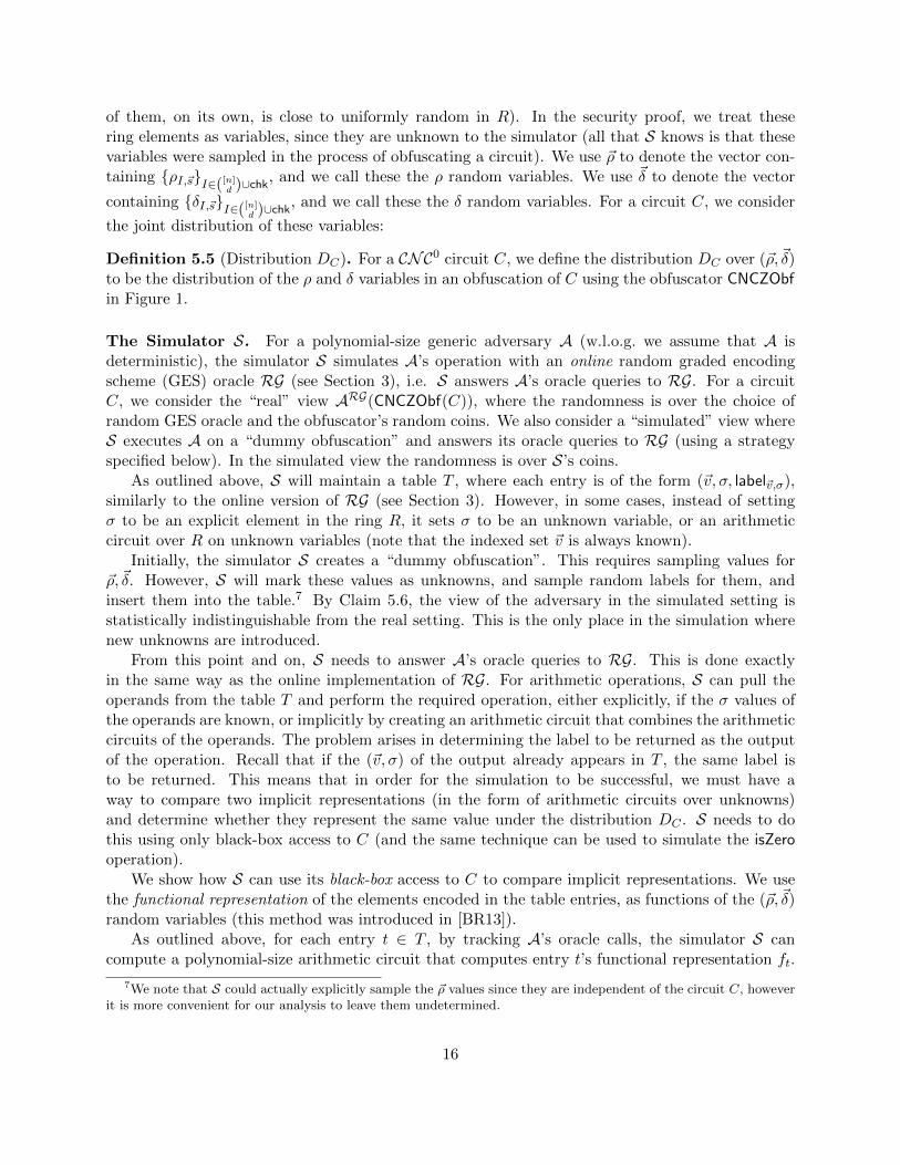
of them, on its own, is close to uniformly random in R). In the security proof, we treat thesering elements as variables, since they are unknown to the simulator (all that S knows is that thesevariables were sampled in the process of obfuscating a circuit). We use ~ρ to denote the vector con-taining ρI,~sI∈([n]

d )∪chk, and we call these the ρ random variables. We use ~δ to denote the vector

containing δI,~sI∈([n]d )∪chk, and we call these the δ random variables. For a circuit C, we consider

the joint distribution of these variables:

Definition 5.5 (Distribution DC). For a CNC0 circuit C, we define the distribution DC over (~ρ, ~δ)to be the distribution of the ρ and δ variables in an obfuscation of C using the obfuscator CNCZObfin Figure 1.

The Simulator S. For a polynomial-size generic adversary A (w.l.o.g. we assume that A isdeterministic), the simulator S simulates A’s operation with an online random graded encodingscheme (GES) oracle RG (see Section 3), i.e. S answers A’s oracle queries to RG. For a circuitC, we consider the “real” view ARG(CNCZObf(C)), where the randomness is over the choice ofrandom GES oracle and the obfuscator’s random coins. We also consider a “simulated” view whereS executes A on a “dummy obfuscation” and answers its oracle queries to RG (using a strategyspecified below). In the simulated view the randomness is over S’s coins.

As outlined above, S will maintain a table T , where each entry is of the form (~v, σ, label~v,σ),similarly to the online version of RG (see Section 3). However, in some cases, instead of settingσ to be an explicit element in the ring R, it sets σ to be an unknown variable, or an arithmeticcircuit over R on unknown variables (note that the indexed set ~v is always known).

Initially, the simulator S creates a “dummy obfuscation”. This requires sampling values for~ρ, ~δ. However, S will mark these values as unknowns, and sample random labels for them, andinsert them into the table.7 By Claim 5.6, the view of the adversary in the simulated setting isstatistically indistinguishable from the real setting. This is the only place in the simulation wherenew unknowns are introduced.

From this point and on, S needs to answer A’s oracle queries to RG. This is done exactlyin the same way as the online implementation of RG. For arithmetic operations, S can pull theoperands from the table T and perform the required operation, either explicitly, if the σ values ofthe operands are known, or implicitly by creating an arithmetic circuit that combines the arithmeticcircuits of the operands. The problem arises in determining the label to be returned as the outputof the operation. Recall that if the (~v, σ) of the output already appears in T , the same label isto be returned. This means that in order for the simulation to be successful, we must have away to compare two implicit representations (in the form of arithmetic circuits over unknowns)and determine whether they represent the same value under the distribution DC . S needs to dothis using only black-box access to C (and the same technique can be used to simulate the isZerooperation).

We show how S can use its black-box access to C to compare implicit representations. We usethe functional representation of the elements encoded in the table entries, as functions of the (~ρ, ~δ)random variables (this method was introduced in [BR13]).

As outlined above, for each entry t ∈ T , by tracking A’s oracle calls, the simulator S cancompute a polynomial-size arithmetic circuit that computes entry t’s functional representation ft.

7We note that S could actually explicitly sample the ~ρ values since they are independent of the circuit C, howeverit is more convenient for our analysis to leave them undetermined.

16

The adversary is limited to multi-linear operations over the inputs, so the functional representationshave very specific cross-linear structure (see below). We use this structure to show that wheneverS needs to check equality of an entry t to 0, S can determine (given the arithmetic circuit thatcomputes ft and black-box access to C) whether w.h.p. over (~ρ, ~δ) ∼ DC , it is the case thatft(~ρ, ~δ) = 0. Similarly, S can use this zero-testing procedure to identify whether two table entriesare equal, by comparing their difference function to 0. This is used to determine whether the outputof a new oracle call to RG is already in the table (and if so, to return its label rather than createa new one). Thus, S can answer all of the adversary’s oracle queries, and generate a statisticallyclose view to the real execution.

The remainder of the proof is organized as follows: first, we formalize the above notions offunctional representations and their structural properties. We then show that for any table entryt, the simulator can determine with high accuracy and in polynomial time whether or not thefunctional representation ft(~ρ, ~δ) equals 0 w.h.p. when (~ρ, ~δ) are drawn from DC . This will allowto complete the simulation as described above. The latter is proven under the bounded speeduphypothesis (Assumption 5.3), which we view as a flavor of the exponential time hypothesis.

5.1 Functional Representations and Structural Properties

We start by exploring the probability space underlying the distribution DC . As explained above,and can be seen from the description of CNCZObf, the ~ρ variables are uniform and independent.The ~δ variables, in contrast, are products of more basic variables. We recall that these variablesinclude:

1. the variables αI,vI∈([n]d ),v∈0,1, which are all uniform and independent in R.

2. The variables βI,i,v, for all i ∈ [n], I 3 i, except the lexicographically first I∗ for each i, andv ∈ 0, 1. These are also uniform and independent (and also independent of the previousvariables). We note that the variables βI∗,i,v are also defined, but are not independent of theother variables, see below.

3. The variables β′ii∈[n] that are also uniform and independent in R (and also independent ofthe previous variables).

Based on these variables, we define βI∗,i,v, for all i, as follows:

βI∗,i,v = β′i ·∏I3i,I 6=I∗

βI,i,1−v .

Note that this implies that βI∗,i,v are uniform subject to the constraint that for all i,∏I3i

βI,i,0 =∏I3i

βI,i,1 (= γi) .

We note the important property that all βI,i,v, β′i, γi variables are completely independent between

different i’s.Finally, δI,~s is defined as

δI,~s = αI,CI(~s) ·∏i∈I

βI,i,~s[i] ,

17

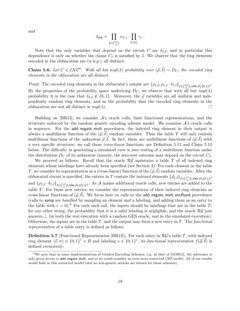
andδchk =

∏I∈([n]

d )

αI,1 ·∏i∈[n]

γi .

Note that the only variables that depend on the circuit C are δI,~s, and in particular thisdependence is only on whether the clause CI is satisfied by ~s. We observe that the ring elementsencoded in the obfuscation are (w.h.p.) all distinct:

Claim 5.6. Let C ∈ CNC0. With all but negl(λ) probability over (~ρ, ~δ) ∼ DC , the encoded ringelements in the obfuscation are all distinct.

Proof. The encoded ring elements in the obfuscator’s output are ρI,~s, ρI,~s · δI,~sI∈([n]d )∪chk,~s∈0,1d .

By the properties of the probability space underlying DC , we observe that with all but negl(λ)probability it is the case that δI,~s 6∈ 0, 1. Moreover, the ~ρ variables are all uniform and inde-pendently random ring elements, and so the probability that the encoded ring elements in theobfuscation are not all distinct is negl(λ).

Building on [BR13], we consider A’s oracle calls, their functional representations, and thestructure enforced by the random generic encoding scheme model. We examine A’s oracle callsin sequence. For the add, negate,mult procedures, the indexed ring element in their output isalways a multilinear function of the (~ρ, ~δ) random variables. Thus the table T will only containmultilinear functions of the unknowns ~ρ, ~δ. In fact, these are multilinear functions of (~ρ, ~δ) witha very specific structure: we call these cross-linear functions, see Definition 5.11 and Claim 5.12below. The difficulty in generating a simulated view is zero testing of a multilinear function underthe distribution DC of its unknowns (namely, the zero-test outcome may depend on the circuit C).

We proceed as follows. Recall that the oracle RG maintains a table T of all indexed ringelements whose labelings have already been specified (see Section 3). For each element in the tableT , we consider its representation as a (cross-linear) function of the (~ρ, ~δ) random variables. After theobfuscated circuit is specified, the entries in T contain the indexed elements ~ρI,~sI∈([n]

d )∪chk,~s∈0,1d

and ρI,~s · δI,~sI∈([n]d )∪chk,~s∈0,1d . As A makes additional oracle calls, new entries are added to the

table T . For these new entries, we consider the representations of their indexed ring elements ascross-linear functions of (~ρ, ~δ). We focus here on calls to the add, negate,mult, encRand procedures(calls to samp are handled by sampling an element and a labeling, and adding them as an entry tothe table with τ = 0).8 For each such call, the inputs should be labelings that are in the table T :for any other string, the probability that it is a valid labeling is negligible, and the oracle RG justanswers ⊥ (in both the real execution with a random GES oracle, and in the simulated execution).Otherwise, the inputs are in the table T , and the output may form a new entry in T . The functionalrepresentation of a table entry is defined as follows.

Definition 5.7 (Functional Representation [BR13]). For each entry in RG’s table T , with indexedring element (~v, σ) ∈ 0, 1τ × R and labeling s ∈ 0, 1∗, its functional representation f(~ρ, ~δ) isdefined recursively:

8We note that in some implementations of Graded Encoding Schemes, e.g. in that of [GGH12], the adversary isonly given access to add, negate,mult, and so we could consider an even more restricted GES model. All of our resultswould hold in this restricted model (and no non-generic attacks are known for those schemes).

18

1. Initially, the only table entries are labelings that appear in the obfuscation. I.e., the entriesfor the ring elements (ρI,~s, (ρI,~s · δI,~s))I∈([n]

d ),~s∈0,1d , where the variables associated with

the index set I are indexed by ~eI . These table entries are all distinct (except with negligibleprobability), and for each table entry its functional representation is simply f(~ρ, ~δ) = ρI,~s or

f(~ρ, ~δ) = (ρI,~s · δI,~s) (respectively).

2. For subsequent entries that are created on A’s calls to RG, their functional representation isdefined recursively. E.g. for an add call, with input labelings s1 and s2, if s1 or s2 is not inRG’s table T , then that input does not represent a valid labeling, the output is ⊥ and no newtable entry is created. If the inputs are in the table T , let (~v1, σ1) and (~v2, σ2) be the indexedring elements that they encode. If ~v1 6= ~v2 then again the output is ⊥ and no new table entryis created. The remaining case is ~v1 = ~v2 = ~v. In this case, let f1 and f2 be the functionalrepresentations of the input labeling. If a new table entry is created for the output, then itsrepresentation is (f1 + f2).

The cases of samp, encRand, negate,mult calls are handled similarly.

We remark that for a table entry t, its functional representation is completely independent ofthe circuit being obfuscated. By definition, the functional representation indeed computes the ringelement in a table entry (for any setting of (~ρ, ~δ)). Moreover, for any table entry, S can computea polynomial-size arithmetic circuit computing that table entry’s functional representation (see[BR13] for the proofs):

Claim 5.8. For any setting of the initial random variables (~ρ, ~δ), and for an entry t in the table Tcontaining the indexed ring element (~vt, σt) and with functional functional representation ft, it isthe case that σt = ft(~ρ, ~δ).

Claim 5.9. For each entry t in RG’s table T , the simulator S can compute a polynomial-sizearithmetic circuit computing its functional representation ft(~ρ, ~α).

As noted above, the functional representations of all table entries are multilinear functions in(~ρ, ~δ). Moreover, they are multilinear functions with a specific structure, defined as cross-linearfunctions in [BR13]. We proceed to define structural properties of these functions, and then usethese to prove security.

Definition 5.10 (cross-linear monomial). A function h(~ρ) is a cross-linear monomial of ~ρ, or aρ-monomial, if it is of the form:

h(~δ) = η · (∏I∈S

ρI,y(I))

where S ⊆(([n]

d

)∪ chk

), y :

(nd

)→ 0, 1d is a partial function defined over S (by notation y(chk)

is the empty string), and η ∈ R. We also say that h is a cross-linear monomial in the variablesρI,y(I)I∈S .

Similarly, a function h(~δ) is a cross-linear monomial of ~δ, or a δ-monomial, if it is of the form:

h(~δ) = η · (∏I∈S

δI,y(I))

where S, y, and η are as above. Similarly to the above, here we say that h is cross-linear in thevariables δI,y(I)I∈S .

19

A cross-linear function in the variables δI,y(I)I∈S is a sum of cross-linear monomials in thesame variables.

Definition 5.11 (cross-linear polynomial [BR13]). A function g(~ρ, ~δ) is a cross-linear term of (~ρ, ~δ)if it is of the form:

g(~ρ, ~δ) = hρ(~ρ) ·

(∑h∈H

h(~δ)

)where hρ is a ρ-monomial (as per Definition 5.10) w.r.t a set S and assignment y, and for eachh ∈ H, h is a δ-monomial over a subset of variables S′ ⊆ S and the assignment y.

A function f is a cross-linear polynomial of (~ρ, ~δ) if it can be expressed as a sum of cross-linearterms. I.e., it is of the form:

f(~ρ, ~δ) =∑g∈G

g(~ρ, ~δ)

where each g ∈ G is a cross-linear term of (~ρ, ~δ) as above. We assume that the expansion is compactin the sense that the for each term g, the set S (of its ρ-monomial) is distinct. We call this particularexpansion the cross-linear expansion of f .

It was shown in [BR13] that in the GES model, the functional representations of all table entriesare cross-linear polynomials:

Claim 5.12. For any entry in the table T , its functional representation is a cross-linear polynomialof (~ρ, ~δ).

5.2 Testing Equality to Zero

For a given table entry t (or difference between table entries), S needs to test whether its functionalrepresentation equals 0. More formally: S wants to test whether it is the case that when (~ρ, ~δ) ∼ DC ,with all but negligible probability the output of ft is zero (we show below that it is always the casethat either ft is always 0, or it is only 0 with negligible probability). We assume that the functionalrepresentation ft(~ρ, ~δ) contains at least one cross-linear term as per Definition 5.11 (otherwise ft istrivially identically 0 under the distribution DC).

At this point we deviate from [BR13], and present a new set of tools. To analyze the possiblestructure of ft, we introduce the notion of consistent assignments, and consistent monomials:

Definition 5.13 (consistent and full assignments). Let y :([n]d

)→ 0, 1d be a partial function

(i.e. one that is not necessarily defined on its entire domain). We say that y is consistent with

~x ∈ 0, 1n, if for all I ∈([n]d

)for which y(I) is defined, it holds that ~x|I = y(I). We say that y is

consistent if it is consistent with some ~x. If y is a total function, we say that it is also full.

Definition 5.14 (full and consistent ρ-monomials). We say that h is a full ρ-monomial if it is aρ-monomial of total degree

(nd

)+1, i.e. of maximal total degree. In this case, for some total function

y :([n]d

)→ 0, 1d, we have h = η ·

((∏I∈(nd)

ρI,y(I)) · ρchk)

. We say that h is the full ρ-monomial

for y. Further, if y is a consistent assignment for some ~x ∈ 0, 1n, as per Definition 5.13, then his a full and consistent ρ-monomial (for the input ~x).

Lemma 5.15 below shows that if ft is not a sum of full and consistent ρ-monomials correspondingto accepting inputs for C (each multiplied by a polynomial in δ), then ft is only 0 with negligibleprobability over DC .

20

The Zero Testing Procedure. The simulator S begins by identifying ρ-monomials of ft. Thiscan be done efficiently by Lemma 5.21. If S finds a non-full or non-consistent monomial, or a fulland consistent monomial for ~x s.t. C(~x) = 0, then by Lemma 5.15 it knows that ft is non-zero(under the distribution DC). If f is a sum of full and consistent ρ-monomials that all correspondto accepting inputs for C (each multiplied by a polynomial in δ), then by Lemma 5.22, S can testwhether ft gets a 0 or non-zero value when (~ρ, ~δ) are drawn by DC .

The only remaining issue is determining whether or not f is a sum of full and consistent ρ-monomials. Lemma 5.21 shows that S can identify any k ρ-monomials of f in time poly(k). Thisis not sufficient, however, because f might be a sum of super polynomially many full and consistentρ-monomials. To rule this out, we show that for an efficient adversary A, with all but negligibleprobability over its coins, all the differences between the functional representations of table entriesthat it creates can only be sums of a polynomial number of full and consistent ρ-monomials. Thisis where we use the bounded-speedup hypothesis.

We show in Lemma 5.18 that any function which is a sum of super-polynomially many full andconsistent ρ-monomials can be used to solve 3-SAT on a super-polynomial set of inputs, which isin contradiction to the BSH (Assumption 5.3). We note that this only requires black-box access tothe functional description.

This finalizes the proof of Theorem 5.1. The formal statements and proof of the aforementionedlemmas follows.

Lemma 5.15. Let C be any CNC0 circuit. Let f be any cross-linear polynomial of (~ρ, ~δ) s.t. f 6≡ 0,where f =

∑g∈G g(~ρ, ~δ), and each function g ∈ G is a cross-linear term (as in Definition 5.11).

If there exists g∗ ∈ G s.t. g∗(~ρ, ~δ) = hρ(~ρ) ·(∑

h∈H h(~δ))

, where hρ is not a full and consistent

ρ-monomial for some input x ∈ 0, 1n s.t. C(x) = 1, then:

Pr(~ρ,~δ)∼DC

[f(~ρ, ~δ) = 0] = negl(λ)

Proof. Consider the monomial g∗ in the lemma statement. Since g∗ is either not full and consistent,or is full and consistent with x such that C(x) = 0, we can apply either Claim 5.16 or Claim 5.17below. We get that the variables ~δ in g∗, when sampled from the distribution DC , are statisticallyclose to being uniform and independent. We can thus apply the Schwatz-Zippel lemma to arguethat with all but negl(λ) probability over ~δ, it holds that

∑h∈H h(~δ) 6= 0. This is because the total

degree of∑

h∈H h(~δ) 6= 0 is at most(nd

)+ 1.

Now, let us consider the function f , restricted to an assignment of all δ variables accordingto DC . This is now a polynomial in the ~ρ variables, with total degree

(nd

)+ 1. Furthermore, this

polynomial is non-zero with all but negligible probability, since the monomial that corresponds to g∗

will not zero out. This implies that by Schwartz-Zippel again, that sampling all ~ρ values accordingto DC (namely, independently and almost uniformly), f(~ρ, ~δ) 6= 0 and the lemma follows.

Claim 5.16. Let y :([n]d

)→ 0, 1d be an assignment that is not consistent or not full. Then the

variables δI,y(I)I∈([n]d )∪chk in DC are negl(λ)-statistically close to uniform and independent.

Proof. We prove that if samp(params) samples labelings of uniform elements in Z∗p (rather than inZp), then the variables stated in the claim are uniform in Z∗p and independent. Since the statisticaldistance from the real setting is (poly(n)/p), the claim follows.

We show two properties:

21

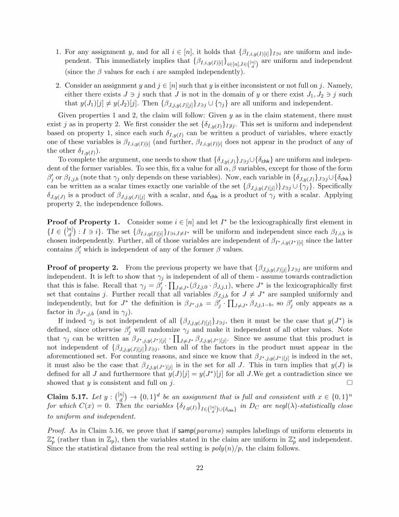
1. For any assignment y, and for all i ∈ [n], it holds that βI,i,y(I)[i]I3i are uniform and inde-pendent. This immediately implies that βI,i,y(I)[i]i∈[n],I∈([n]

d ) are uniform and independent

(since the β values for each i are sampled independently).

2. Consider an assignment y and j ∈ [n] such that y is either inconsistent or not full on j. Namely,either there exists J 3 j such that J is not in the domain of y or there exist J1, J2 3 j suchthat y(J1)[j] 6= y(J2)[j]. Then βJ,j,y(J)[j]J3j ∪ γj are all uniform and independent.

Given properties 1 and 2, the claim will follow: Given y as in the claim statement, there mustexist j as in property 2. We first consider the set δI,y(I)I 63j . This set is uniform and independentbased on property 1, since each such δI,y(I) can be written a product of variables, where exactlyone of these variables is βI,i,y(I)[i] (and further, βI,i,y(I)[i] does not appear in the product of any ofthe other δI,y(I)).

To complete the argument, one needs to show that δJ,y(J)J3j∪δchk are uniform and indepen-dent of the former variables. To see this, fix a value for all α, β variables, except for those of the formβ′j or βI,j,b (note that γj only depends on these variables). Now, each variable in δJ,y(J)J3j∪δchkcan be written as a scalar times exactly one variable of the set βJ,j,y(J)[j])J3j ∪ γj. SpecificallyδJ,y(J) is a product of βJ,j,y(J)[j] with a scalar, and δchk is a product of γj with a scalar. Applyingproperty 2, the independence follows.

Proof of Property 1. Consider some i ∈ [n] and let I∗ be the lexicographically first element in

I ∈([n]d

): I 3 i. The set βI,i,y(I)[i]I3i,I 6=I∗ will be uniform and independent since each βI,i,b is

chosen independently. Further, all of those variables are independent of βI∗,i,y(I∗)[i] since the lattercontains β′i which is independent of any of the former β values.

Proof of property 2. From the previous property we have that βJ,j,y(J)[j]J3j are uniform andindependent. It is left to show that γj is independent of all of them - assume towards contradictionthat this is false. Recall that γj = β′j ·

∏J 6=J∗(βJ,j,0 · βJ,j,1), where J∗ is the lexicographically first

set that contains j. Further recall that all variables βJ,j,b for J 6= J∗ are sampled uniformly andindependently, but for J∗ the definition is βJ∗,j,b = β′j ·

∏J 6=J∗ βJ,j,1−b, so β′j only appears as a

factor in βJ∗,j,b (and in γj).If indeed γj is not independent of all βJ,j,y(J)[j]J3j , then it must be the case that y(J∗) is

defined, since otherwise β′j will randomize γj and make it independent of all other values. Notethat γj can be written as βJ∗,j,y(J∗)[j] ·

∏J 6=J∗ βJ,j,y(J∗)[j]. Since we assume that this product is

not independent of βJ,j,y(J)[j]J3j , then all of the factors in the product must appear in theaforementioned set. For counting reasons, and since we know that βJ∗,j,y(J∗)[j] is indeed in the set,it must also be the case that βJ,j,y(J∗)[j] is in the set for all J . This in turn implies that y(J) isdefined for all J and furthermore that y(J)[j] = y(J∗)[j] for all J .We get a contradiction since weshowed that y is consistent and full on j.

Claim 5.17. Let y :([n]d

)→ 0, 1d be an assignment that is full and consistent with x ∈ 0, 1n

for which C(x) = 0. Then the variables δI,y(I)I∈([n]d )∪δchk

in DC are negl(λ)-statistically close

to uniform and independent.

Proof. As in Claim 5.16, we prove that if samp(params) samples labelings of uniform elements inZ∗p (rather than in Zp), then the variables stated in the claim are uniform in Z∗p and independent.Since the statistical distance from the real setting is poly(n)/p, the claim follows.

22

We show that:

• Letting y, x be as in the claim statement, the variables αI,CI(x) ∪ ∏I αI,1 are all uniform

and independent.

The claim immediately follows since even conditioned on all the β values, each δI,y(I) a productthat contains αI,CI(x), and δchk is a product that contains

∏I αI,1.

The proof of the above property is also fairly straightforward. Since C(x) = 0, there exists Jsuch that αJ,CJ (x) = αJ,0. Now, all αI,CI(x) are independent by definition (since they are sampledindependently), and

∏I αI,1 is independent of all of them since it is a product that contains αJ,1.

Lemma 5.18. For n, λ ∈ N, and X ⊆ 0, 1n, let f be any cross-linear function of (~ρ, ~δ) s.t.

f =∑x∈X

hx(~ρ) · gx(~δ)

where ∀x ∈ X, hx is a full ρ-monomial which is consistent with x, and gx 6≡ 0.Then there exists a polynomial-size circuit Af s.t. for any circuit B ∈ CNC0 on n-bit inputs,

the circuit Af on input B decides whether there exist x ∈ X that satisfies B. I.e.:

∀B ∈ CNC0 : PrA

[A(B) = 1∃x∈X:B(x)=1] ≥ 1− negl(λ)

Proof. Each hx(~ρ) is a full ρ-monomial consistent with x, and so:

∀x ∈ X : hx(~ρ) =∏

I∈(([n]

d )∪chk) ~ρI,x|I

The algorithm Af picks (~ρ, ~δ) from a distribution FB, which depends on the circuit B (but isnot the distribution DB that these variables take in the obfuscation). Af outputs 1 iff f(~ρ, ~δ) 6= 0.The distribution FB is obtained as follows: each variable in ~δ is chosen uniformly and random fromthe ring. For each variable ρI,~s, if BI(~s) = 1 then it is chosen uniformly at random, but if BI(~s) = 0then it is always fixed to 0. The variable ~ρchk is uniformly random and independent. The lemmafollows from Claims 5.19 and 5.20 below.

Claim 5.19. If ∀x ∈ X,B(x) = 0, then Pr~ρ,~δ

[f(~ρ, ~δ) = 0] = 1

Proof. Since ∀x ∈ X,B(x) = 0, we conclude that ∀x ∈ X,∃I ∈([n]d

): BI(x|I) = 0. By the

construction of FB, we conclude that ∀x ∈ X,∃I ∈([n]d

): ρI,x|I = 0. Thus ∀x ∈ X, the function

hx(~ρ), which is a product of all of the ρI,x|I variables, outputs 0. We conclude that f(~ρ, ~δ) =∑x∈X hx(~ρ) · gx(~δ) is a sum of 0’s, and so when f ’s input is drawn from DF , f ’s output is always

0.

Claim 5.20. If ∃x∗ ∈ X : B(x∗) = 1, then Pr~ρ,~δ

[f(~ρ, ~δ) = 0] = negl(λ).

23

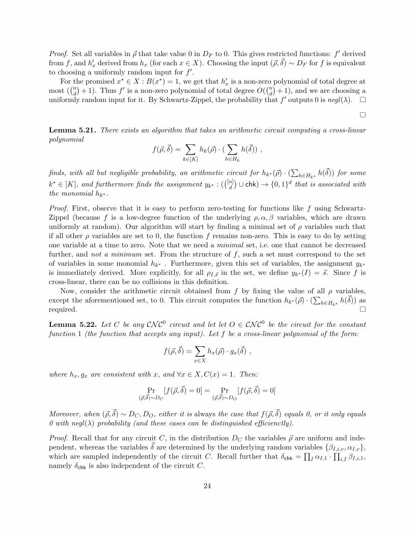
Proof. Set all variables in ~ρ that take value 0 in DF to 0. This gives restricted functions: f ′ derivedfrom f , and h′x derived from hx (for each x ∈ X). Choosing the input (~ρ, ~δ) ∼ DF for f is equivalentto choosing a uniformly random input for f ′.

For the promised x∗ ∈ X : B(x∗) = 1, we get that h′x is a non-zero polynomial of total degree atmost (

(nd

)+ 1). Thus f ′ is a non-zero polynomial of total degree O(

(nd

)+ 1), and we are choosing a

uniformly random input for it. By Schwartz-Zippel, the probability that f ′ outputs 0 is negl(λ).

Lemma 5.21. There exists an algorithm that takes an arithmetic circuit computing a cross-linearpolynomial

f(~ρ, ~δ) =∑k∈[K]

hk(~ρ) · (∑h∈Hk

h(~δ)) ,

finds, with all but negligible probability, an arithmetic circuit for hk∗(~ρ) · (∑

h∈Hk∗h(~δ)) for some

k∗ ∈ [K], and furthermore finds the assignment yk∗ : (([n]d

)∪ chk)→ 0, 1d that is associated with

the monomial hk∗.

Proof. First, observe that it is easy to perform zero-testing for functions like f using Schwartz-Zippel (because f is a low-degree function of the underlying ρ, α, β variables, which are drawnuniformly at random). Our algorithm will start by finding a minimal set of ρ variables such thatif all other ρ variables are set to 0, the function f remains non-zero. This is easy to do by settingone variable at a time to zero. Note that we need a minimal set, i.e. one that cannot be decreasedfurther, and not a minimum set. From the structure of f , such a set must correspond to the setof variables in some monomial hk∗ . Furthermore, given this set of variables, the assignment yk∗

is immediately derived. More explicitly, for all ρI,~s in the set, we define yk∗(I) = ~s. Since f iscross-linear, there can be no collisions in this definition.

Now, consider the arithmetic circuit obtained from f by fixing the value of all ρ variables,except the aforementioned set, to 0. This circuit computes the function hk∗(~ρ) · (

∑h∈Hk∗

h(~δ)) asrequired.

Lemma 5.22. Let C be any CNC0 circuit and let let O ∈ CNC0 be the circuit for the constantfunction 1 (the function that accepts any input). Let f be a cross-linear polynomial of the form:

f(~ρ, ~δ) =∑x∈X

hx(~ρ) · gx(~δ) ,

where hx, gx are consistent with x, and ∀x ∈ X,C(x) = 1. Then:

Pr(~ρ,~δ)∼DC

[f(~ρ, ~δ) = 0] = Pr(~ρ,~δ)∼DO

[f(~ρ, ~δ) = 0]

Moreover, when (~ρ, ~δ) ∼ DC , DO, either it is always the case that f(~ρ, ~δ) equals 0, or it only equals0 with negl(λ) probability (and these cases can be distinguished efficienctly).

Proof. Recall that for any circuit C, in the distribution DC the variables ~ρ are uniform and inde-pendent, whereas the variables ~δ are determined by the underlying random variables βI,i,v, αI,v,which are sampled independently of the circuit C. Recall further that δchk =

∏I αI,1 ·

∏i,I βI,i,1,

namely δchk is also independent of the circuit C.

24

In contrast, for all I, ~s, δI,~s = αI,CI(~s) ·∏i∈I βI,i,~s[i]. I.e. these variables do depend on the circuit

C and differ between DC and DO. However, since f is a sum of (products of) monomials that areconsistent with accepting inputs of C, it follows that all of the δ variables in f are consistent withan accepting input x: i.e. they are of the form δI,~s, where there exists an input x ∈ X s.t. C(x) = 1and x|I = ~s, so it must be the case that CI(~s) = 1. In other words, for all δ values in f , it holdsthat

δI,~s = αI,CI(~s) ·∏i∈I

βI,i,~s[i] = αI,1 ·∏i∈I

βI,i,~s[i] = αI,OI(~s) ·∏i∈I

βI,i,~s[i] ,

Thus, the joint distributions of the δ variables in DC and DO are identical. The Lemma followsbecause, viewing f(~ρ, ~δ) as a function of the ρ, α, β variables (the same function when (~ρ, ~δ) aredrawn from DC or from DO), either f is always 0, or it is only 0 with negligible probability (bySchwartz-Zippel, since f is a low-degree function of the uniformly random ρ, α, β).

Acknowledgments. We thank Shafi Goldwasser for helpful and insightful comments, and MoniNaor for bring to our attention the connections between the Bounded Speedup Hypothesis andparameterized complexity theory. We are grateful to Ryan Williams for illuminating conversationsabout the Bounded Speedup Hypothesis, and in particular for pointing out the proof that qBSHis implied by ETH [Wil13]. We also thank Amir Yehudayoff for helpful discussions on arithmeticcircuit complexity.

References

[AW07] Ben Adida and Douglas Wikstrom. How to shuffle in public. In Salil P. Vadhan, editor,TCC, volume 4392 of Lecture Notes in Computer Science, pages 555–574. Springer,2007.

[BC10] Nir Bitansky and Ran Canetti. On strong simulation and composable point obfuscation.In CRYPTO, pages 520–537, 2010.

[BGI+12] Boaz Barak, Oded Goldreich, Russell Impagliazzo, Steven Rudich, Amit Sahai, Salil P.Vadhan, and Ke Yang. On the (im)possibility of obfuscating programs. J. ACM, 59(2):6,2012. Preliminary version in CRYPTO 2001.

[BR13] Zvika Brakerski and Guy Rothblum. Obfuscating conjunctions, 2013. To appear inCRYPTO 2013.

[BS02] Dan Boneh and Alice Silverberg. Applications of multilinear forms to cryptography.IACR Cryptology ePrint Archive, 2002:80, 2002.

[Can97] Ran Canetti. Towards realizing random oracles: Hash functions that hide all partialinformation. In CRYPTO, pages 455–469, 1997.

[CD08] Ran Canetti and Ronny Ramzi Dakdouk. Obfuscating point functions with multibitoutput. In EUROCRYPT, pages 489–508, 2008.

[CLT13] Jean-Sebastien Coron, Tancrede Lepoint, and Mehdi Tibouchi. Practical multilinearmaps over the integers. Cryptology ePrint Archive, Report 2013/183, 2013. To appearin CRYPTO 2013.

25

[CMR98] Ran Canetti, Daniele Micciancio, and Omer Reingold. Perfectly one-way probabilistichash functions (preliminary version). In STOC, pages 131–140, 1998.

[CRV10] Ran Canetti, Guy N. Rothblum, and Mayank Varia. Obfuscation of hyperplane mem-bership. In TCC, pages 72–89, 2010.

[DS05] Yevgeniy Dodis and Adam Smith. Correcting errors without leaking partial information.In Harold N. Gabow and Ronald Fagin, editors, STOC, pages 654–663. ACM, 2005.

[FG06] J. Flum and M. Grohe. Parameterized Complexity Theory. Springer, 2006.

[GGH12] Sanjam Garg, Craig Gentry, and Shai Halevi. Candidate multilinear maps from ideallattices and applications. IACR Cryptology ePrint Archive, 2012:610, 2012. To appearin EUROCRYPT 2013.

[GGH+13] Sanjam Garg, Craig Gentry, Shai Halevi, Mariana Raykova, Amit Sahai, and BrentWaters. Candidate indistinguishability obfuscation and functional encryption for allcircuits. Cryptology ePrint Archive, Report 2013/451, 2013. To appear in FOCS 2013.

[GK05] Shafi Goldwasser and Yael Tauman Kalai. On the impossibility of obfuscation withauxiliary input. In FOCS, pages 553–562, 2005.

[GR07] Shafi Goldwasser and Guy N. Rothblum. On best-possible obfuscation. In Salil P.Vadhan, editor, TCC, volume 4392 of Lecture Notes in Computer Science, pages 194–213. Springer, 2007.

[HMLS10] Dennis Hofheinz, John Malone-Lee, and Martijn Stam. Obfuscation for cryptographicpurposes. J. Cryptology, 23(1):121–168, 2010.

[HRSV11] Susan Hohenberger, Guy N. Rothblum, Abhi Shelat, and Vinod Vaikuntanathan. Se-curely obfuscating re-encryption. J. Cryptology, 24(4):694–719, 2011.

[IP99] Russell Impagliazzo and Ramamohan Paturi. Complexity of k-sat. In IEEE Conferenceon Computational Complexity, pages 237–240. IEEE Computer Society, 1999.

[LPS04] Ben Lynn, Manoj Prabhakaran, and Amit Sahai. Positive results and techniques forobfuscation. In EUROCRYPT, pages 20–39, 2004.

[Mau05] Ueli . Maurer. Abstract models of computation in cryptography. In IMA Int. Conf.,pages 1–12, 2005.

[Nao03] Moni Naor. On cryptographic assumptions and challenges. In Dan Boneh, editor,CRYPTO, volume 2729 of Lecture Notes in Computer Science, pages 96–109. Springer,2003.

[Rot13] Ron Rothblum. On the circular security of bit-encryption. In TCC, pages 579–598,2013.

[Sho97] Victor Shoup. Lower bounds for discrete logarithms and related problems. In EURO-CRYPT, pages 256–266, 1997.

26

[Wee05] Hoeteck Wee. On obfuscating point functions. In Harold N. Gabow and Ronald Fagin,editors, STOC, pages 523–532. ACM, 2005.

[Wil13] Ryan Williams. Personal communication, 2013.

A The Bounded Speedup Hypothesis

In this section we investigate the relation between BSH and ETH. We use an insight of Williams[Wil13] to show that qBSH (quasi-polynomial BSH) is in fact implied by ETH. We also discuss aconnection with parameterized complexity. We start by restating BSH, qBSH, ETH using similarterminology.

Definition 5.2 (X -3-SAT solver, restated). Consider a family of sets X = Xnn∈N such thatXn ⊆ 0, 1n. We say that an algorithm A is a X -3-SAT solver if it solves the 3-SAT problem,restricted to inputs in X . Namely, given a 3-CNF formula Φ : 0, 1n → 0, 1, A finds whetherthere exists x ∈ Xn such that Φ(x) = 1.

Assumption 5.3 (BSH, restated). There exists a polynomial p(·), such that for any X -3-SATsolver that runs in time t(·), the family of sets X is of size at most p(t(·)).

The quasi-BSH (qBSH), is a variant where the polynomial p(·) is allowed to have degree log(n).

Assumption 5.4 (qBSH restated). For any X -3-SAT solver that runs in time t(n), the family ofsets X is of size at most (t(n))O(log(n)).

We proceed with the exponential time hypothesis, presented by Impagliazzo and Paturi [IP99].For our purposes, we use the weaker notion of ETH (the strong version makes claims about kCNF-SAT for all k).

Assumption A.1 (The Exponential Time Hypothesis). There is no 2o(n)-time 0, 1n-3-SATsolver.

We further consider the following scaled down version of the ETH, which is not stronger thanthe original.

Assumption A.2 (Scaled-Down ETH). There is no t(n)-time solver for ω(log(t(n)))-variable 3-SAT.

Assumption A.1 implies Assumption A.2 by a scaling argument. The Scalded-Down ETH, inturn, is more similar to the BSH: we can view a solver for ω(log(n))-variable 3SAT as an X solverwhere X covers all possible assignments of the first ω(log(n)) variables (or rather, any subset ofω(log(n)) variables). The only difference from BSH thus is that the family X is “structured” inthe sense of being concentrated on a small set of coordinates.

In fact, when we consider non-uniform solvers, the ETH implies qBSH (note that the scalingdown above also applies to non-uniform solvers):

Lemma A.3 ([Wil13]). For non-uniform solvers, qBSH is implied by Scaled-Down ETH for (andtherefore, qBSH is implied by ETH for non-uniform circuits).

27

Proof. We start by recalling a learning theoretic argument. Given a family X , we can consider thestrings in Xn as functions in 0, 1k → 0, 1, where k = dlog(n)e (the (2k−n) last bits can be set tozero). Recall that by Sauer’s Lemma, the VC dimension of Xn (as a set of boolean functions) is atleast dim = Ω(log(|Xn|)/k). This means that there exists a set of dim coordinates that is shutteredby Xn. Namely, such that there exists 2dim functions in Xn that cover all possible assignments tothis set of coordinates.

It follows, therefore, that if there exists a X -3-SAT solver A that runs in time t(n) with |Xn| =(t(n))ω(log(n)), then there is a set of

Ω(log(|Xn|)/dlog(n)e) = ω(log(t(n)))

coordinates that is shuttered by Xn (namely, they take all possible assignments when ranging overXn). Mapping those to the variables of a scaled-down formula, yields a (non-uniform) solver forthe Scaled-Down ETH (the coordinates to map to are specified by non-uniform advice).

Connections with Parameterized Complexity. The bounded-speedup hypothesis impliesthat 3-SAT is hard even when restricted to super-polynomial-size subsets of inputs. One naturalset to consider is the inputs of weight k, where k is super-constant or logarithmic (and weight isthe L1 norm, or the number of 1’s in the assignment). This is a super-polynomial set, with a veryshort implicit description.

The problems of resolving SAT and 3-SAT on inputs of weight k, in time that is f(k) · poly(n)(for any function f , even super-exponential in k), has been studied in the context of parameterizedcomplexity. “Weighted” 3-SAT is known to be complete for the class W [1], and is not generallybelieved to be tractable. See e.g. [FG06].

This study shows an obstacle to finding a 3-SAT algorithm with significant speedup for everyset X of inputs: in particular, doing so for the set of low-weight inputs seems hard. Still, weemphasize the Bounded Speedup Hypothesis asks for more: it says that there exists no set withsuper-polynomial speedup. Reducing this hypothesis to a more well studied worst-case problem isan intriguing direction for future work.

28