Bivariate factorizations via Galois theory,with application to exceptional polynomials

Michael Zieve∗

Hill Center, Department of Mathematics, Rutgers University,110 Frelinghuysen Road, Piscataway NJ 08854

zieve@math.rutgers.edu

Abstract

We present a method for factoring polynomials of the shape f(X)−f(Y ), where f is a univariate polynomial over a field k. We then applythis method in the case when f is a member of the infinite family ofexceptional polynomials we discovered jointly with H. Lenstra in 1995;factoring f(X)−f(Y ) in this case was posed as a problem by S. Cohenshortly after the discovery of these polynomials.

1 Introduction

Factoring polynomials is one of the classical problems in algebra. Thereis of course an algorithmic aspect to this problem, but our concern is amore theoretical one: how can one factor each member of an infinite familyof polynomials? It seems that the literature contains rather little aboutthis problem in the case of polynomials in more than one variable, and infact contains few examples. In this paper we describe a general method forfactoring polynomials of the shape f(X) − f(Y ), where f is a univariatepolynomial over a field k, which is often successful even when f varies overan infinite family of polynomials. More precisely, we expose a connectionwith group theory which reduces the problem of factoring f(X) − f(Y ) to

∗The author’s work supported by an NSF postdoctoral fellowship

1

certain computations in the Galois group of f(X) − t over k(t), where t isan indeterminate. Our results are related to work of Abhyankar (cf. [1]–[3] among various other papers) in which he goes in the opposite direction,deriving information about Galois groups of polynomials from the shapes offactorizations such as the ones in the present paper.

To illustrate our method, we use it to factor f(X)−f(Y ) for a certain fam-ily of polynomials for which these factorizations are particularly important,namely certain exceptional polynomials f . Here a polynomial f(X) ∈ k[X] iscalled exceptional if there are no irreducible factors of f(X)−f(Y ) in k[X, Y ],other than (multiples of) X−Y , which remain irreducible over the algebraicclosure of k (i.e. which are absolutely irreducible). Exceptional polynomialshave a rich theory and possess several interesting properties. For instance, apolynomial f over a finite field k is exceptional if and only if there is an infi-nite algebraic extension ` of k for which the map f : `→ ` given by a 7→ f(a)is bijective (i.e. f is a permutation polynomial over `). A primer on excep-tional polynomials is included as an appendix to this paper. Over the yearsnumerous authors have contributed to the theory of exceptional polynomi-als, with steady success, but a radical change in perspective came in 1993.This was due to the work of Fried, Guralnick and Saxl [9], who used hardgroup theory (including the classification of finite simple groups) in order toseverely restrict the possibilities for the Galois group Gal(f(X) − t, k(t)) ofan exceptional polynomial. Their work provided hope for a complete clas-sification of exceptional polynomials, something which previously had notbeen dreamt possible. The thrust of their result is that the Galois groupis typically an affine group (that is, a group of invertible affine transfor-mations of a vector space), except for certain unexpected possibilities overfields of characteristic two and three. Every exceptional polynomial known in1993 had affine Galois group; but following [9] there was a flurry of activitywhich saw the construction of new (non-affine) exceptional polynomials incharacteristics two and three. In fact, in recent work Guralnick and I havecompletely classified the non-affine exceptional polynomials [13]. However,for the non-affine exceptional polynomials in characteristic three (which werediscovered jointly with Lenstra [15]), the exceptionality property was provenindirectly, without deriving the factorization of f(X)− f(Y ), and up to nowthis factorization has not been known (although it is clearly important, sinceit is the main ingredient in the definition of exceptionality; also it is used inthe above-mentioned paper [13]). In this paper we produce this factorizationby applying our general method for factoring bivariate polynomials of this

2

shape.Let us sketch the method. Consider a monic polynomial f(X) ∈ k[X],

where to ease the exposition we make the minor assumption that f ′(X) 6= 0.Assume that we know the normal closure Ω of the field extension k(y)/k(t),where t = f(y) and y is transcendental over k, and that we know the groupG = Gal(Ω/k(t)). First we compute the subdegrees of G, namely the indices[Gy : Gxy] where x varies over the G-conjugates of y and Gy denotes thesubgroup of G fixing y. Next, for each x we produce a polynomial over k(y),having x as a root, which has degree [Gy : Gxy]; this polynomial will be theminimal polynomial of x over k(y), and as such is an irreducible factor off(X) − f(y) in k[X, y]. Then f(X) − f(y) is the product of the distinctirreducibles gotten in this manner (since polynomials of this shape cannothave multiple roots). The second step will provide the most difficulties ingeneral: it requires us to produce a polynomial of prescribed degree havingx as a root. In our example this arises in Section 6, where the shape ofthe roots x in our case suggests the form of the desired polynomials; this iscertainly the prettiest part of the argument.

Since it is significant for the theory of exceptional polynomials, we now de-scribe the explicit factorization we produce as an illustration of our method.We work with the infinite family of (indecomposable) exceptional polynomi-als over F3 from [15]; these are members of a more general family of polyno-mials having fairly uniform properties, defined as follows: if q ≡ 3 (mod 4)is a power of a prime p, and d divides (q + 1)/4, there is a correspondingpolynomial in Fp[X],

fq,d = X(X2d + 1)(q+1)/(4d)

((X2d + 1)(q−1)/2 − 1

X2d

)(q+1)/(2d)

.

We present the factorization of fq,d(X)− fq,d(Y ) over Fp[X, Y ] for arbitraryd and q > 3; from these factorizations one immediately sees that fq,d isexceptional over Fp precisely when p = 3, and one can also read off variousother properties of the fq,d.

In his talk at the Third International Conference on Finite Fields and Ap-plications (Glasgow 1995), S. Cohen asked for the factorization of fq,d(X)−fq,d(Y ); this motivated the present work. In that talk Cohen also presentedtwo polynomials of degree (q + 1)/4 which he conjectured should be factorsof fq,(q+1)/4 (based on evidence from a computer search); the validation of hisconjecture is one consequence of our work.

3

The factorizations involve the Dickson polynomials, which are defined asfollows: for any positive integer n, any field k, and any a ∈ k, the Dick-son polynomial of degree n having parameter a is the unique polynomialDn(X, a) ∈ k[X] for which Dn(Y + (a/Y ), a) = Y n + (a/Y )n. Now pute = (q + 1)/(4d). The polynomial fq,d(X) − fq,d(Y ) ∈ Fp[X,Y ] is the prod-uct of X − Y and several other distinct irreducibles R(X, Y ) ∈ Fp[X, Y ], ofwhich two have degree (q + 1)/4, and (q − 3)/2 have degree (q + 1)/2, and(q− 3)/4 have degree q+ 1. The two factors R(X,Y ) of degree (q+ 1)/4 aredetermined by the choice of

√−1; these R satisfy

R(Xe, Y e) =∏ζe=1

(Y (q+1)/4D(q+1)/4 (ζX/Y + 1/2, 1/16) +

√−1).

The factors R(X, Y ) of degree (q + 1)/2 are determined by the choices of φand µ, where φ is a nonsquare in Fq of the form θ2 + θ with θ ∈ Fq \ −1/2,and µ ∈ Fq2 satisfies µ2 = φ; these R satisfy

R(X2e, Y 2e) =∏ζ2e=1

(Y (q+1)/2D(q+1)/2 (ζX/Y − 1− 2θ, φ) + 2µ

).

Here the choice of θ is irrelevant. The factors R(X, Y ) of degree q + 1 aredetermined by the choice of a nonzero square φ ∈ Fq having the form θ2 + θfor some θ ∈ Fq; here we have

R(X2e, Y 2e) =∏ζ2e=1

(Y q+1Dq+1 (ζX/Y − 1− 2θ, φ)− φ(2Y q+1 + 4)

).

Again, the choice of θ is irrelevant.We will also use our method to derive the factorization of f(X)− f(Y ),

where f(X) is one of the non-affine exceptional polynomials in characteristictwo which were discovered by Cohen and Matthews following examples ofMuller. This factorization appeared in [5], where it was verified by entirelydifferent methods after having been conjectured based on bits of evidencecoming from a number of different directions. Our approach, based on theGalois-theoretic information from [12], provides new insight into this factor-ization; for instance, we resolve a mystery from [5]. This mystery is thatthe factors of f(X)− f(Y ) can be expressed in terms of Dickson polynomi-als (just as is true for the odd characteristic polynomials above); in [5], theDickson polynomials entered only at the very last step, as a way of rewrit-ing the factorization after all proofs had been completed. In our approach

4

the Dickson polynomials arise naturally out of the dihedral groups which arepoint-stabilizers of the Galois groups. Another advantage of our approachis that the factorization is derived rather than verified; this differs from [5],where the proofs will only work if the factorization has been conjectured atthe outset (our approach produces the factors themselves by pure reasoning,with no need for guesswork).

We now describe the contents of this paper in more detail. In the nextsection we explain the general factorization method. In Section 3 we recallknown facts about the specific polynomials fq,d, which we require in order tofactor fq,d(X)−fq,d(Y ). Then in the next three sections we apply our methodto produce this bivariate factorization, first computing the subdegrees of theappropriate group, next computing the roots of fq,d(X) − t, and then pro-ducing the factors themselves. Section 7 contains some consequences of thefactorization, and discusses the role of the factorization in the theory of thefq,d. After giving a quick primer on exceptional polynomials in Appendix A,we conclude in Appendix B by applying our method to derive the bivariatefactorizations associated to the Muller-Cohen-Matthews exceptional polyno-mials.

It is a pleasure to thank Hendrik W. Lenstra, Jr. for several valuableconversations, and Stephen D. Cohen for comments on an earlier version ofthis manuscript.

Notation. In the various sections of this paper (but not in the appendices)we keep certain notational conventions. As above, q ≡ 3 (mod 4) is a powerof a prime p. For E ∈ Fq2 , we let E := Eq denote the conjugate of E in theextension Fq2/Fq. The algebraic closure of a field k is denoted k. Finally, wereserve α for a fixed square root of −1 in Fq2 , and d for a divisor of (q+1)/4,and put e = (q + 1)/(4d).

2 General method

In this section we explain our approach to factoring polynomials f(X)−f(Y ).We start by reformulating the problem via some easy reductions. Let f(X) bea polynomial in k[X]; without loss we assume f monic. We reserve the lettersX, Y for indeterminates, transcendental over every field under consideration;to avoid confusion, we will write y for Y whenever we want to view it asan element of a prescribed field (but always y is transcendental over k, so

5

the factorizations of f(X) − f(y) and f(X) − f(Y ) over k differ only bythe substitution of Y for y). When viewed as a member of k[y][X], thepolynomial f(X) − f(y) is monic (in X), so we may assume that each ofits irreducible factors in k[y][X] is also monic in X. Then each of thesefactors is irreducible in k(y)[X] (by Gauss’ lemma), so it suffices to find thefactorization of f(X) − f(y) into monic irreducible polynomials R(X, y) ∈k(y)[X] (each such R will necessarily lie in k[y][X]).

Next we reduce to the case where the factors R are distinct. Note thatf ′(X) = 0 if and only if f is a polynomial in Xp, where p = char(k); equiva-lently, f(X) = h(X)p for some polynomial h(X) ∈ k[X] (where h(X) ∈ k[X]if k perfect), i.e. f(X) − f(y) = (h(X) − h(y))p. It follows that, at leastin the case of perfect fields k, in order to factor f(X) − f(y) it is sufficientto perform the factorization under the assumption that f ′(X) 6= 0 (and forimperfect k we can first perform the factorization over the perfect field kand then piece together the factorization over k). Henceforth, to simplifythe exposition, we assume f ′(X) 6= 0; this implies that f(X) − f(y) has nomultiple roots (as any such root x would satisfy f ′(x) = 0, so x ∈ k, whencef(y) = f(x) ∈ k, contradicting the fact that y is transcendental over k).Thus, f(X) − f(y) is the product of its distinct monic irreducible factorsR(X, y) ∈ k(y)[X], and we have only to find these factors.

Now put t = f(y), so that f(X) − f(y) = f(X) − t. As above, thispolynomial over k(t) is separable (since f ′(X) 6= 0) and irreducible (by Gauss’lemma). Let G = Gal(f(X) − t, k(t)) be its Galois group. One root off(X)− t is y; the other roots are the k(t)-conjugates of y, namely the valuesτ(y) for τ ∈ G. Thus, the monic irreducible factors of f(X) − t in k(y)[X]are precisely the minimal polynomials over k(y) of the various τ(y).

Our first step in the construction of these minimal polynomials will bethe computation of their degrees. We translate this to a group theoreticcalculation. Let H be the subgroup of G consisting of elements fixing y. Forany τ ∈ G, the subgroup of G consisting of elements fixing τ(y) is Hτ :=τHτ−1. By Galois theory, the degree of the minimal polynomial of τ(y) overk(y), or [k(τ(y), y) : k(y)], equals the index [H : H ∩Hτ ] = #H/#(H ∩Hτ ).(In group theoretic terms, these indices are the subdegrees of the transitivepermutation group G.) Thus, to compute the degrees, we must determinethe sizes of the various intersections H ∩Hτ .

In the example considered in this paper, we perform this computationin Section 4. Then we explicitly compute the various τ(y), after which weproduce their minimal polynomials. But first, in the next section, we recall

6

the details of this example.

3 Galois theory of the fq,d

In this section we review some known properties (from [15]) of the specialclass of polynomials fq,d to be considered in this paper. We begin with thepolynomials f = fq,1. Recall that q ≡ 3 (mod 4) is a power of a prime p, andthat f(X) ∈ Fp[X] is given by

f(X) = X(X2 + 1)(q+1)/4

((X2 + 1)(q−1)/2 − 1

X2

)(q+1)/2

.

We take a ‘top-down’ approach to the Galois-theoretic setup of f , as donein [15] and similar to Serre’s appendix to [1]; this means that we start withthe largest field to be considered, which will turn out to be the splittingfield of f(X) − t, and produce all smaller fields as fixed fields of groups ofautomorphisms of the large field. In our case, we begin with the field Fp(v),where v is transcendental over Fp (and Fp is an algebraic closure of Fp).The group PGL2(Fp) acts as a group of automorphisms of Fp(v), with thematrix

(A BC D

)corresponding to the Fp-automorphism of Fp(v) sending v to

(Av + C)/(Bv + D); in fact, any Fp-automorphism of Fp(v) has this form.The subfield of Fp(v) fixed (elementwise) by the group G′ = PSL2(Fq) isFp(t), where

t = (−1)(q+1)/4α(vq

2 − v)(q+1)/2

(vq − v)(q2+1)/2;

here α denotes a square root of −1. Let H ′ be the subgroup of G′ given by

H ′ =

(A B−εB εA

): A,B ∈ Fq, ε ∈ ±1, A2 +B2 = ε

/±I,

where I =(

1 00 1

)is the identity; then H ′ is a dihedral group of order q + 1.

The subfield of Fp(v) fixed by H ′ is Fp(y), where

y = α(v2 + 1)(q+1)/2

vq − v.

Then Fp(v) is the Galois closure of the separable extension Fp(y)/Fp(t), andmoreover t = f(y). By Galois theory, G′ (respectively, H ′) is the subgroup

7

of PGL2(Fp) ∼= AutFp

(Fp(v)) consisting of elements fixing t (respectively, y);

also Fp(v) is the splitting field of f(X)− t over Fp(t).For the purposes of the present paper, it is convenient to modify the above

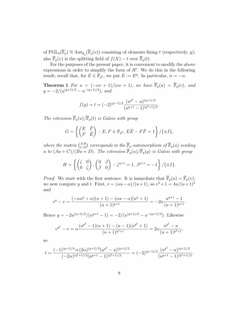
expressions in order to simplify the form of H ′. We do this in the followingresult; recall that, for E ∈ Fq2 , we put E := Eq. In particular, α = −α.

Theorem 1 For u = (−αv + 1)/(αv + 1), we have Fp(u) = Fp(v), andy = −2/(u(q+1)/2 − u−(q+1)/2), and

f(y) = t = (−2)(p−1)/2 (uq2 − u)(q+1)/2

(uq+1 − 1)(q2+1)/2.

The extension Fp(u)/Fp(t) is Galois with group

G =

(E FF E

): E,F ∈ Fq2 , EE − FF = 1

/±I,

where the matrix(ABC D

)corresponds to the Fp-automorphism of Fp(u) sending

u to (Au+ C)/(Bu+D). The extension Fp(u)/Fp(y) is Galois with group

H =

(ζ 00 ζ

),

(0 ββ 0

): ζq+1 = 1, βq+1 = −1

/±I.

Proof. We start with the first sentence. It is immediate that Fp(u) = Fp(v);we now compute y and t. First, v = (αu−α)/(u+1), so v2 +1 = 4u/(u+1)2

and

vq − v =(−αuq + α)(u+ 1)− (αu− α)(uq + 1)

(u+ 1)q+1= −2α

uq+1 − 1

(u+ 1)q+1.

Hence y = −2u(q+1)/2/(uq+1 − 1) = −2/(u(q+1)/2 − u−(q+1)/2). Likewise

vq2 − v = α

(uq2 − 1)(u+ 1)− (u− 1)(uq

2+ 1)

(u+ 1)q2+1= 2α

uq2 − u

(u+ 1)q2+1,

so

t =(−1)(q+1)/4 α (2α)(q+1)/2(uq

2 − u)(q+1)/2

(−2α)(q2+1)/2(uq+1 − 1)(q2+1)/2= (−2)(p−1)/2 (uq

2 − u)(q+1)/2

(uq+1 − 1)(q2+1)/2.

8

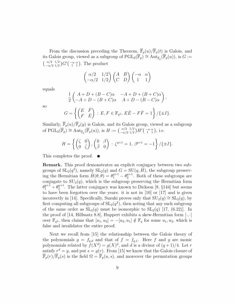
From the discussion preceding the Theorem, Fp(u)/Fp(t) is Galois, andits Galois group, viewed as a subgroup of PGL2(Fp) ∼= Aut

Fp(Fp(u)), is G :=( α/2 1/2

−α/2 1/2

)G′( −α α

1 1

). The product(

α/2 1/2−α/2 1/2

)(A BC D

)(−α α1 1

)equals

1

2

(A+D + (B − C)α −A+D + (B + C)α−A+D − (B + C)α A+D − (B − C)α

),

so

G =

(E FF E

): E,F ∈ Fq2 , EE − FF = 1

/±I.

Similarly, Fp(u)/Fp(y) is Galois, and its Galois group, viewed as a subgroup

of PGL2(Fp) ∼= AutFp

(Fp(u)), is H :=( α/2 1/2−α/2 1/2

)H ′( −α α

1 1

), i.e.

H =

(ζ 00 ζ

),

(0 ββ 0

): ζq+1 = 1, βq+1 = −1

/±I.

This completes the proof.

Remark. This proof demonstrates an explicit conjugacy between two sub-groups of SL2(q2), namely SL2(q) and G = SU(q, H), the subgroup preserv-ing the Hermitian form H(θ, θ) = θq+1

1 − θq+12 . Both of these subgroups are

conjugate to SU2(q), which is the subgroup preserving the Hermitian formθq+1

1 + θq+12 . The latter conjugacy was known to Dickson [8, §144] but seems

to have been forgotten over the years: it is not in [10] or [17] and is givenincorrectly in [14]. Specifically, Suzuki proves only that SU2(q) ∼= SL2(q), byfirst computing all subgroups of SL2(q2), then noting that any such subgroupof the same order as SL2(q) must be isomorphic to SL2(q) [17, (6.22)]. Inthe proof of [14, Hilfssatz 8.8], Huppert exhibits a skew-Hermitian form [·, ·]over Fq2 , then claims that [u1, u2] = −[u2, u1] /∈ Fq for some u1, u2, which isfalse and invalidates the entire proof.

Next we recall from [15] the relationship between the Galois theory ofthe polynomials g = fq,d and that of f = fq,1. Here f and g are monicpolynomials related by f(Xd) = g(X)d, and d is a divisor of (q+ 1)/4. Let rsatisfy rd = y, and put s = g(r). From [15] we know that the Galois closure ofFp(r)/Fp(s) is the field Ω = Fp(u, s), and moreover the permutation groups

9

G = Gal(Ω/Fp(s)) = Gal(g(X) − s,Fp(s)) and G = Gal(Fp(u)/Fp(t)) =Gal(f(X) − t,Fp(t)) are isomorphic (via the restriction map); also Fp(r) =

Fp(y, s), so the subgroup H of G consisting of elements fixing r corresponds

to H. For σ ∈ G, the subgroup of G fixing σ(r) is Hσ = σHσ−1; if τ ∈ G isthe projection of σ, then this group corresponds to Hτ . It follows that theintersection H ∩ Hσ has the same size as H ∩Hτ , so the minimal polynomialof σ(r) over Fp(r) has the same degree as the minimal polynomial of τ(y) overFp(y). In the next section we compute these degrees for the various rootsτ(y) of f(X)− t, thereby finding them for the roots σ(r) of g(X)− s; afterthat we compute the minimal polynomials for the various σ(r) to producethe desired bivariate factorization.

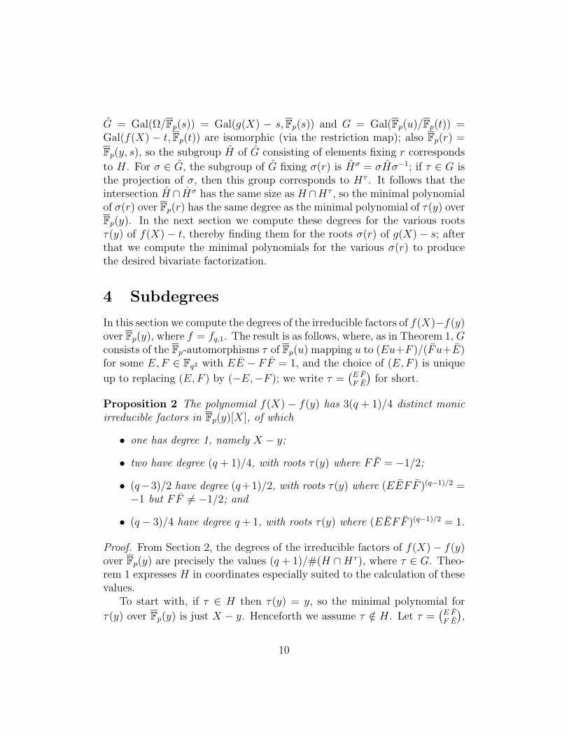
4 Subdegrees

In this section we compute the degrees of the irreducible factors of f(X)−f(y)over Fp(y), where f = fq,1. The result is as follows, where, as in Theorem 1, Gconsists of the Fp-automorphisms τ of Fp(u) mapping u to (Eu+F )/(F u+E)for some E,F ∈ Fq2 with EE − FF = 1, and the choice of (E,F ) is unique

up to replacing (E,F ) by (−E,−F ); we write τ =(E FF E

)for short.

Proposition 2 The polynomial f(X) − f(y) has 3(q + 1)/4 distinct monicirreducible factors in Fp(y)[X], of which

• one has degree 1, namely X − y;

• two have degree (q + 1)/4, with roots τ(y) where FF = −1/2;

• (q−3)/2 have degree (q+1)/2, with roots τ(y) where (EEF F )(q−1)/2 =−1 but FF 6= −1/2; and

• (q − 3)/4 have degree q + 1, with roots τ(y) where (EEF F )(q−1)/2 = 1.

Proof. From Section 2, the degrees of the irreducible factors of f(X)− f(y)over Fp(y) are precisely the values (q + 1)/#(H ∩Hτ ), where τ ∈ G. Theo-rem 1 expresses H in coordinates especially suited to the calculation of thesevalues.

To start with, if τ ∈ H then τ(y) = y, so the minimal polynomial for

τ(y) over Fp(y) is just X − y. Henceforth we assume τ /∈ H. Let τ =(E FF E

),

10

where E,F ∈ Fq2 with EE − FF = 1; then our assumption simply assertsthat EF 6= 0.

We now compute H∩Hτ for τ /∈ H. One easily checks that no nonidentitydiagonal matrices in H have diagonal conjugate by τ ; that no diagonal matrixin H has antidiagonal conjugate by τ , unless FF = −1/2 (in which casethere is one such diagonal matrix); and that no antidiagonal matrix in H hasantidiagonal conjugate, unless (EEF F )(q−1)/2 = −1, in which case there aretwo such antidiagonal matrices. Hence, #H ∩Hτ is 4 if FF = −1/2, is 2 if(EEF F )(q−1)/2 = −1 and FF 6= −1/2, and is 1 if (EEF F )(q−1)/2 = 1. Thusthe degree of the minimal polynomial for τ(y) over Fp(y) in these cases is(q + 1)/4 or (q + 1)/2 or q + 1, respectively.

Now that we know the possible sizes of H ∩Hτ , we compute the numberof τ ’s for which each size occurs. Note that the preimage of any elementof F∗q under the (q + 1)-th power map F∗q2 → F

∗q has size q + 1. Thus the

first case occurs for (q + 1)2/2 choices of τ (equivalently, choices of (E,F )up to the equivalence (E,F ) ∼ (−E,−F )); dividing by #H = q + 1 gives(q+ 1)/2 conjugates of t having minimal polynomial of degree (q+ 1)/4, andsince all the roots of any such minimal polynomial are conjugates of t, wefind that there are two polynomials in this case. To count the polynomialsin the other cases, note that θ := FF = EE − 1 is an arbitrary element ofFq\0,−1,−1/2, and EEF F = θ2+θ is a square in Fq for precisely half of allsuch values θ (as can be proven by classical elementary arguments involvingthe quadratic character). Thus, the second case occurs for (q − 3)(q + 1)2/4choices of τ , hence for (q − 3)(q + 1)/4 conjugates of t and finally thereare (q − 3)/2 polynomials in this case. The third case occurs for the samenumber of τ ’s as does the second, hence occurs for (q − 3)/4 polynomials.This completes the proof.

5 Computation of roots

In this section we compute the values σ(r) where σ ∈ G. As before, e =

(q + 1)/(4d). Let σ correspond to(E FF E

)∈ G, where E,F ∈ Fq2 satisfy

EE − FF = 1; the result is as follows.

Proposition 3 We have σ(r) = rw2e and σ(y) = yw(q+1)/2, where

w = EFu+ EFu−1 + EE + FF .

11

Proof. We start with σ(y). Theorem 1 implies y = −2/(u(q+1)/2− u−(q+1)/2);it follows that

σ(y) =−2((Eu+ F )(F u+ E)

)(q+1)/2

(Eu+ F )q+1 − (F u+ E)q+1.

We compute (Eu + F )q+1 = (Euq + F )(Eu + F ) = EEuq+1 + EFuq +EFu+ FF ; since (F u+ E)q+1 is gotten by switching E and F in the aboveexpression, we find that (Eu+ F )q+1 − (F u+ E)q+1 = uq+1 − 1. Thus

σ(y) =−2(EFu+ (EE + FF ) + EFu−1

)(q+1)/2

u(q+1)/2 − u−(q+1)/2= yw(q+1)/2.

Since σ(r)d = σ(y) = yw(q+1)/2 = rdw(q+1)/2, we have σ(r) = rw2eη whereηd = 1; we must show that η = 1 (note that this is certainly true whenEF = 0; henceforth we assume EF 6= 0). Since s = g(r) is fixed by σ, wehave g(r) = g(σ(r)), so

r(r2d + 1)e(

(r2d + 1)(q−1)/2 − 1

r2d

)2e

=

σ(r) · (σ(r)2d + 1)e(

(σ(r)2d + 1)(q−1)/2 − 1

σ(r)2d

)2e

;

substituting σ(r)d = rdw(q+1)/2 and σ(r) = rw2eη (and rd = y) gives

(y2 + 1)e(

(y2 + 1)(q−1)/2 − 1

y2

)2e

=

ηw2e(y2wq+1 + 1)e(

(y2wq+1 + 1)(q−1)/2 − 1

y2wq+1

)2e

.

Thus for some ξ with ξe = η we have

(y2+1)

((y2 + 1)(q−1)/2 − 1

y2

)2

= ξw2(y2wq+1+1)

((y2wq+1 + 1)(q−1)/2 − 1

y2wq+1

)2

;

multiplying by y4w2q gives

(∗) w2q((y2 + 1)q − 2(y2 + 1)(q+1)/2 + (y2 + 1)

)= ξ

((y2wq+1 + 1)q − 2(y2wq+1 + 1)(q+1)/2 + (y2wq+1 + 1)

).

12

Recall that w = (EFu2+(EE+FF )u+EF )/u and y = −2u(q+1)/2/(uq+1−1);when we make these substitutions in (∗), and multiply both sides by thequantity u2q(uq+1−1)2q, we get an equality of elements of Fp[u]. To determineξ, it suffices to compare the leading coefficients of the resulting polynomials.After a straightforward computation one finds that these leading coefficientsare 4(EF )2 and 4ξ(EF )2, so ξ = 1 and thus η = ξe = 1 as desired. Finally,σ(r) = rw2e.

6 Minimal polynomials

For each σ ∈ G \ H, we can now determine a monic polynomial in Fp(r)[X],of the appropriate degree, which has σ(r) as a root; this will be the minimalpolynomial for σ(r) over Fp(r). Once we have computed these minimal poly-nomials, the factorization stated in the introduction will follow at once fromthe discussion in Section 2.

As in the previous section, let σ correspond to(E FF E

)∈ G, where E,F ∈

Fq2 satisfy EE − FF = 1, and let γ = EEF F . By Proposition 3, we haverd = y = −2/(u(q+1)/2−u−(q+1)/2) and σ(r) = rw2e and w = EFu+EFu−1 +(EE + FF ). The shape of w is suggestive of the Dickson polynomials; weclarify this in each of the cases of Proposition 2. For each choice of σ, thatresult tells us the degree n of σ(r) over Fp(r); for each σ we produce threepolynomials over Fp(r), each of degree n. The first polynomial has w as aroot, the second has w2e as a root, and the third has σ(r) as a root (and thethird is monic). The first has the shape P (X) = bDn(X−(EE+FF ), γ)+c,where Dn(Z, γ) is a Dickson polynomial and b, c ∈ Fp(r). The second isdefined by Q(X2e) =

∏ζ2e=1 P (ζX). The third is just R(X) = Q(X/r).

Actually, for the two factors of degree (q + 1)/4, we will have to deviateslightly from this plan, but we still follow the same general strategy. In thenext three paragraphs we implement this plan for each of the three nontrivialcases in Proposition 2.

First assume FF = −1/2 (so EE = 1/2). Then

D(q+1)/2(w,−1/4) = D(q+1)/2

(EFu− (4EFu)−1,−1/4

)= (EFu)(q+1)/2 + (4EFu)−(q+1)/2;

since (EF )q+1 = −1/4, this last expression equals

(EF )(q+1)/2(u(q+1)/2 − u−(q+1)/2) = −2(EF )(q+1)/2/rd.

13

Thus w is a root of P (X) = rdD(q+1)/2(X,−1/4) + 2(EF )(q+1)/2 ∈ Fp(r)[X];

to get a polynomial of degree (q+1)/4 from this, we note that P (X) = P (X2)for some P (X) ∈ Fp(r)[X], where P (w2) = 0. Define Q(X) ∈ Fp(r)[X] byQ(Xe) =

∏ζe=1 P (ζX), so w2e is a root of Q; then R(X) = Q(X/r) ∈

Fp(r)[X] vanishes at rw2e = σ(r). Here R is monic of degree (q + 1)/4, soindeed R is the minimal polynomial for σ(r) over Fp(r). The polynomialsP,Q,R are determined by the value of 2(EF )(q+1)/2 = ±α, yielding at mosttwo polynomials R; since there are indeed two factors in this case, thesepolynomials are distinct.

Next assume γ(q−1)/2 = −1 but FF 6= −1/2. Then

D(q+1)/2

(w − (EE + FF ), γ

)= (EFu)(q+1)/2 +

γ(q+1)/2

(EFu)(q+1)/2;

this last is just (EF )(q+1)/2(u(q+1)/2−u−(q+1)/2) = −2(EF )(q+1)/2/rd. Thus wis a root of P (X) = rdD(q+1)/2

(X − (EE + FF ), γ

)+2(EF )(q+1)/2, so w2e is

a root of the polynomial Q(X) defined by Q(X2e) =∏

ζ2e=1 P (ζX). Finally,

σ(r) = rw2e is a root of R(X) = Q(X/r). Here R is a monic polynomialin Fp(r)[X] of degree (q + 1)/2, so R is the minimal polynomial for σ(r)over Fp(r). The polynomials P,Q,R are determined by the values of FFand (EF )(q+1)/2; here θ := FF ∈ Fq \ −1/2 satisfies (θ2 + θ)(q−1)/2 = −1,and (EF )(q+1)/2 is a square root of θ2 + θ. Thus there are (q − 3)/2 choicesfor θ, each of which corresponds to two values of (EF )(q+1)/2; however, thepolynomials Q corresponding to θ and −θ − 1 are identical, so there are atmost (q−3)/2 distinct polynomials R in this case. Again, we know there areprecisely this many factors in this case, so these polynomials are distinct.

Now assume γ(q−1)/2 = 1. Then

Dq+1

(w − (EE + FF ), γ

)= γ

(uq+1 + u−(q+1)

)= γ(4r−2d + 2),

so w is a root of P (X) = r2dDq+1

(X − (EE + FF ), γ

)− γ(2r2d + 4). Put

Q(X2e) =∏

ζ2e=1 P (ζX), so Q(w2e) = 0, and thus σ(r) is a root of R(X) =

Q(X/r). Since R is a monic polynomial in Fp(r)[X] of degree q + 1, againit is the minimal polynomial for σ(r) over Fp(r). The polynomials P,Q,Rare determined by the value of θ := FF ; this is an element of Fq satisfying(θ2 + θ)(q−1)/2 = 1. There are (q − 3)/2 such values θ; however, replacing θby −θ− 1 leaves Q and R unchanged, so there are at most (q− 3)/4 distinctpolynomials R in this case. As above, since this equals the number of factorsin this case, these polynomials are distinct.

14

In summary, the polynomial g(X)−g(r) ∈ Fp(r)[X] is the product ofX−rand several other distinct irreducibles, two of which have degree (q + 1)/4,(q− 3)/2 of which have degree (q+ 1)/2, and (q− 3)/4 of which have degreeq+1. The two factors R(X) of degree (q+1)/4 are determined by the choiceof√−1; for ze = r these R satisfy

R(Xe) =∏ζe=1

(z(q+1)/4D(q+1)/2

(√ζX/z,−1/4

)+√−1).

Here the choice of√ζX/z is irrelevant, since D(q+1)/2 is an even function.

The factors R(X) of degree (q + 1)/2 are determined by the choices of anonsquare element φ ∈ Fq of the form θ2 + θ with θ ∈ Fq \ −1/2, andµ ∈ Fq2 with µ2 = φ; here, for z2e = r,

R(X2e) =∏ζ2e=1

(z(q+1)/2D(q+1)/2 (ζX/z − 1− 2θ, φ) + 2µ

).

Here the choice of θ is irrelevant. The factors R(X) of degree q + 1 aredetermined by the choice of a nonzero square φ ∈ Fq having the form θ2 + θfor some θ ∈ Fq; for z2e = r we have

R(X2e) =∏ζ2e=1

(zq+1Dq+1 (ζX/z − 1− 2θ, φ)− φ(2zq+1 + 4)

).

Again, the choice of θ is irrelevant. Finally, one can make use of the well-known trivial relation Dmn(X, a) = Dn(Dm(X, a), am) to rewrite the degree(q + 1)/4 factors in the form given in the introduction.

7 Consequences of the factorization

In this section we note some consequences of the factorization proved above.In particular, we show that certain known properties of the fq,d follow atonce from the bivariate factorization; this factorization provides new per-spective on the known results, and we hope that this new perspective mightlead to new results in the future. We begin by determining when fq,d isexceptional (over Fp). To this end, note that each of the factors R(X, Y )we have presented is monic in X (that is, monic when viewed as a mem-ber of Fp[Y ][X]); thus, if no R(X, Y ) lies in Fp[X, Y ], then also no scalar

15

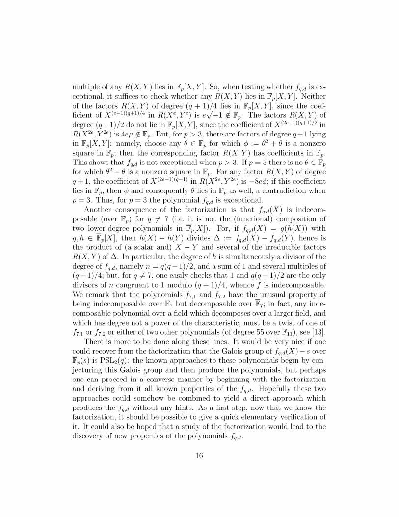
multiple of any R(X, Y ) lies in Fp[X,Y ]. So, when testing whether fq,d is ex-ceptional, it suffices to check whether any R(X, Y ) lies in Fp[X,Y ]. Neitherof the factors R(X, Y ) of degree (q + 1)/4 lies in Fp[X,Y ], since the coef-ficient of X(e−1)(q+1)/4 in R(Xe, Y e) is e

√−1 /∈ Fp. The factors R(X, Y ) of

degree (q+1)/2 do not lie in Fp[X, Y ], since the coefficient of X(2e−1)(q+1)/2 inR(X2e, Y 2e) is 4eµ /∈ Fp. But, for p > 3, there are factors of degree q+1 lyingin Fp[X, Y ]: namely, choose any θ ∈ Fp for which φ := θ2 + θ is a nonzerosquare in Fp; then the corresponding factor R(X,Y ) has coefficients in Fp.This shows that fq,d is not exceptional when p > 3. If p = 3 there is no θ ∈ Fpfor which θ2 + θ is a nonzero square in Fp. For any factor R(X,Y ) of degreeq+ 1, the coefficient of X(2e−1)(q+1) in R(X2e, Y 2e) is −8eφ; if this coefficientlies in Fp, then φ and consequently θ lies in Fp as well, a contradiction whenp = 3. Thus, for p = 3 the polynomial fq,d is exceptional.

Another consequence of the factorization is that fq,d(X) is indecom-posable (over Fp) for q 6= 7 (i.e. it is not the (functional) composition oftwo lower-degree polynomials in Fp[X]). For, if fq,d(X) = g(h(X)) withg, h ∈ Fp[X], then h(X) − h(Y ) divides ∆ := fq,d(X) − fq,d(Y ), hence isthe product of (a scalar and) X − Y and several of the irreducible factorsR(X,Y ) of ∆. In particular, the degree of h is simultaneously a divisor of thedegree of fq,d, namely n = q(q−1)/2, and a sum of 1 and several multiples of(q+ 1)/4; but, for q 6= 7, one easily checks that 1 and q(q− 1)/2 are the onlydivisors of n congruent to 1 modulo (q + 1)/4, whence f is indecomposable.We remark that the polynomials f7,1 and f7,2 have the unusual property ofbeing indecomposable over F7 but decomposable over F7; in fact, any inde-composable polynomial over a field which decomposes over a larger field, andwhich has degree not a power of the characteristic, must be a twist of one off7,1 or f7,2 or either of two other polynomials (of degree 55 over F11), see [13].

There is more to be done along these lines. It would be very nice if onecould recover from the factorization that the Galois group of fq,d(X)−s overFp(s) is PSL2(q): the known approaches to these polynomials begin by con-jecturing this Galois group and then produce the polynomials, but perhapsone can proceed in a converse manner by beginning with the factorizationand deriving from it all known properties of the fq,d. Hopefully these twoapproaches could somehow be combined to yield a direct approach whichproduces the fq,d without any hints. As a first step, now that we know thefactorization, it should be possible to give a quick elementary verification ofit. It could also be hoped that a study of the factorization would lead to thediscovery of new properties of the polynomials fq,d.

16

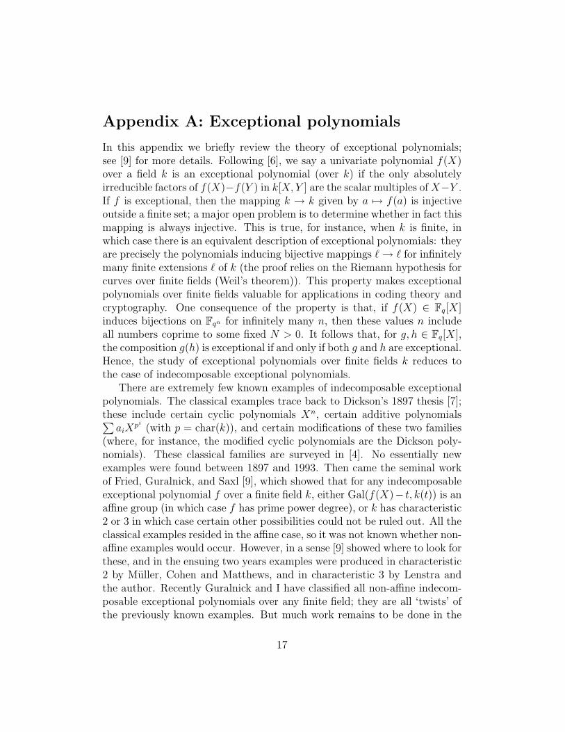
Appendix A: Exceptional polynomials

In this appendix we briefly review the theory of exceptional polynomials;see [9] for more details. Following [6], we say a univariate polynomial f(X)over a field k is an exceptional polynomial (over k) if the only absolutelyirreducible factors of f(X)−f(Y ) in k[X, Y ] are the scalar multiples of X−Y .If f is exceptional, then the mapping k → k given by a 7→ f(a) is injectiveoutside a finite set; a major open problem is to determine whether in fact thismapping is always injective. This is true, for instance, when k is finite, inwhich case there is an equivalent description of exceptional polynomials: theyare precisely the polynomials inducing bijective mappings `→ ` for infinitelymany finite extensions ` of k (the proof relies on the Riemann hypothesis forcurves over finite fields (Weil’s theorem)). This property makes exceptionalpolynomials over finite fields valuable for applications in coding theory andcryptography. One consequence of the property is that, if f(X) ∈ Fq[X]induces bijections on Fqn for infinitely many n, then these values n includeall numbers coprime to some fixed N > 0. It follows that, for g, h ∈ Fq[X],the composition g(h) is exceptional if and only if both g and h are exceptional.Hence, the study of exceptional polynomials over finite fields k reduces tothe case of indecomposable exceptional polynomials.

There are extremely few known examples of indecomposable exceptionalpolynomials. The classical examples trace back to Dickson’s 1897 thesis [7];these include certain cyclic polynomials Xn, certain additive polynomials∑aiX

pi (with p = char(k)), and certain modifications of these two families(where, for instance, the modified cyclic polynomials are the Dickson poly-nomials). These classical families are surveyed in [4]. No essentially newexamples were found between 1897 and 1993. Then came the seminal workof Fried, Guralnick, and Saxl [9], which showed that for any indecomposableexceptional polynomial f over a finite field k, either Gal(f(X)− t, k(t)) is anaffine group (in which case f has prime power degree), or k has characteristic2 or 3 in which case certain other possibilities could not be ruled out. All theclassical examples resided in the affine case, so it was not known whether non-affine examples would occur. However, in a sense [9] showed where to look forthese, and in the ensuing two years examples were produced in characteristic2 by Muller, Cohen and Matthews, and in characteristic 3 by Lenstra andthe author. Recently Guralnick and I have classified all non-affine indecom-posable exceptional polynomials over any finite field; they are all ‘twists’ ofthe previously known examples. But much work remains to be done in the

17

affine case; new examples were exhibited by Guralnick and Muller [11], butthere will probably be many further examples and it is not clear whether itis feasible to classify them all.

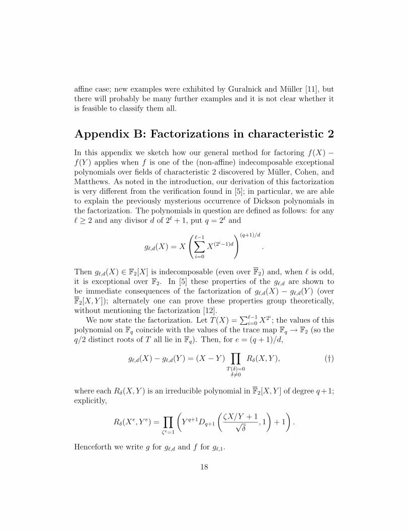
Appendix B: Factorizations in characteristic 2

In this appendix we sketch how our general method for factoring f(X) −f(Y ) applies when f is one of the (non-affine) indecomposable exceptionalpolynomials over fields of characteristic 2 discovered by Muller, Cohen, andMatthews. As noted in the introduction, our derivation of this factorizationis very different from the verification found in [5]; in particular, we are ableto explain the previously mysterious occurrence of Dickson polynomials inthe factorization. The polynomials in question are defined as follows: for any` ≥ 2 and any divisor d of 2` + 1, put q = 2` and

g`,d(X) = X

(`−1∑i=0

X(2i−1)d

)(q+1)/d

.

Then g`,d(X) ∈ F2[X] is indecomposable (even over F2) and, when ` is odd,it is exceptional over F2. In [5] these properties of the g`,d are shown tobe immediate consequences of the factorization of g`,d(X) − g`,d(Y ) (overF2[X, Y ]); alternately one can prove these properties group theoretically,without mentioning the factorization [12].

We now state the factorization. Let T (X) =∑`−1

i=0 X2i ; the values of this

polynomial on Fq coincide with the values of the trace map Fq → F2 (so theq/2 distinct roots of T all lie in Fq). Then, for e = (q + 1)/d,

g`,d(X)− g`,d(Y ) = (X − Y )∏

T (δ)=0δ 6=0

Rδ(X, Y ), (†)

where each Rδ(X, Y ) is an irreducible polynomial in F2[X, Y ] of degree q+1;explicitly,

Rδ(Xe, Y e) =

∏ζe=1

(Y q+1Dq+1

(ζX/Y + 1√

δ, 1

)+ 1

).

Henceforth we write g for g`,d and f for g`,1.

18

We begin by computing the degrees of the irreducible factors of g(X) −g(Y ) in F2[X,Y ]. As in Section 2, g(X) − g(Y ) is the product of severaldistinct irreducible factors, whose degrees are the subdegrees of the permu-tation group Gal(g(X) − s,F2(s)). This group is isomorphic to PGL2(q) inits transitive permutation representation with one-point stabilizer a dihedralgroup of order q + 1. One computes the subdegrees in a manner similar tothat of Section 4, and finds that they are all q + 1 except a single one whichis one (corresponding to the factor X − Y ).

Next we compute the roots of g(X)−s. From [12], for t = sd the splittingfield of f(X)− t over F2(t) is F2(u), and the splitting field of g(X)− s overF2(s) is F2(u, s). The restriction map induces an isomorphism between G :=Gal(F2(u, s)/F2(s)) and Gal(F2(u)/F2(t)), where the elements of the lattergroup are the F2-isomorphisms of F2(u) sending u to (Eu + F )/(F u + E),for any choice of E,F ∈ Fq2 such that EE + FF = 1 (here E := Eq). Oneroot r ∈ F2(u, s) of g(X) − s satisfies r−d = uq+1 + u−(q+1); the other rootsare the images of r under G, which we compute (as in Section 5) to be rwe

for e = (q + 1)/d and w = 1 + EFu+ EFu−1.Finally we compute the minimal polynomials over F2(r) for these roots.

Assume rwe 6= r. Put γ = EEF F . Then w is a root of the polynomialP (X) = Dq+1(X+1, γ)+γr−d. Next, we is a root of Q(X) ∈ F2(r)[X] defined

by Q(Xe) =∏

ζe=1 P (ζX). Thus rwe is a root of R(X) = rq+1Q(X/r), which

is a monic polynomial in F2(r)[X] of degree q + 1, hence is the minimalpolynomial for rwe over F2(r). Note that R is determined by the value of γ,and γ = θ2 + θ for θ := FF ∈ F∗q; hence T (γ) = 0. Now denoting R(X) by

Rδ(X), it follows that

g(X)− g(r) = (X − r)∏

T (δ)=0δ 6=0

Rδ(X).

It remains to recover Rδ(X, Y ) from Rδ(X). For ze = r, note that g(Xe)−g(ze) = g(Xe) − s is the product of Xe − Y e and the various Rδ(X

e), eachof which is monic and irreducible in F2(r)[Xe]. But

Rδ(Xe) = rq+1

∏ζe=1

P (ζX/z) =∏ζe=1

(zq+1Dq+1(ζX/z + 1, γ) + γ

)lies in F2[re, Xe]; substituting Y for z and X for Xe, we see that g(X) −g(Y ) = (X − Y )

∏δ Rδ(X, Y ), where Rδ is the irreducible polynomial in

19

F2[X, Y ] defined by

Rδ(Xe, Y e) =

∏ζe=1

(Y q+1Dq+1(ζX/Y + 1, γ) + γ

).

Standard trivial properties of Dickson polynomials imply that Rδ is a scalarmultiple of Rδ, which completes our derivation of the factorization (†).

Note that g`,d(X) = X−qT (Xd)(q+1)/d; such a simple expression for g`,dseems to merit a better explanation than is presently known.

References

[1] S. S. Abhyankar, Galois theory on the line in nonzero characteristic,Bull. Amer. Math. Soc. 27 (1992), 68–133.

[2] S. S. Abhyankar, Nice equations for nice groups, Israel J. Math. 88(1994), 1–24.

[3] S. S. Abhyankar, S. D. Cohen, and M. E. Zieve, Bivariate factorizationsconnecting Dickson polynomials and Galois theory, Trans. Amer. Math.Soc., to appear.

[4] S. D. Cohen, Exceptional polynomials and the reducibility of substitu-tion polynomials, Enseign. Math. 36 (1990), 53–65.

[5] S. D. Cohen and R. M. Matthews, Exceptional polynomials, Finite FieldsAppl. 1 (1995), 261–277.

[6] H. Davenport and D. J. Lewis, Notes on Congruences (I), Quart. J.Math. Oxford, Ser. 2, 14 (1963), 51–60.

[7] L. E. Dickson, The analytic representation of substitutions on a power ofa prime number of letters with a discussion of the linear group, AnnalsMath. 11 (1897), 65–120.

[8] L. E. Dickson, “Linear groups with an exposition of the Galois fieldtheory,” 1901 (reprinted Dover, New York, 1958).

[9] M. D. Fried, R. M. Guralnick, and J. Saxl, Schur covers and Carlitz’sconjecture, Israel J. Math. 82 (1993), 157–225.

20

[10] D. Gorenstein, “Finite groups,” Harper&Row, New York, 1968.

[11] R. M. Guralnick and P. Muller, Exceptional polynomials of affine type,J. Algebra 194 (1997), 429–454.

[12] R. M. Guralnick and M. Zieve, Exceptional rational functions of smallgenus, in preparation.

[13] R. M. Guralnick and M. Zieve, Polynomials with prescribed monodromy,preprint.

[14] B. Huppert, “Endliche gruppen,” Springer-Verlag, Berlin, 1967.

[15] H. W. Lenstra, Jr. and M. Zieve, A family of exceptional polynomials, in“Finite Fields and Applications,” pp. 209–218, Cambridge Univ. Press,Cambridge, 1996.

[16] H. W. Lenstra, Jr. and M. Zieve, Exceptional maps between varieties,in preparation.

[17] M. Suzuki, “Group theory. I.,” Springer-Verlag, New York, 1982.

21