Embed Size (px)
Citation preview

General rights Copyright and moral rights for the publications made accessible in the public portal are retained by the authors and/or other copyright owners and it is a condition of accessing publications that users recognise and abide by the legal requirements associated with these rights.
• Users may download and print one copy of any publication from the public portal for the purpose of private study or research. • You may not further distribute the material or use it for any profit-making activity or commercial gain • You may freely distribute the URL identifying the publication in the public portal
If you believe that this document breaches copyright please contact us providing details, and we will remove access to the work immediately and investigate your claim.
Downloaded from orbit.dtu.dk on: Sep 08, 2018
Bisphenol A and its structural analogues in household waste paper
Pivnenko, Kostyantyn; Pedersen, Gitte Alsing; Eriksson, Eva; Astrup, Thomas Fruergaard
Published in:Waste Management
Link to article, DOI:10.1016/j.wasman.2015.07.017
Publication date:2015
Document VersionPeer reviewed version
Link back to DTU Orbit
Citation (APA):Pivnenko, K., Pedersen, G. A., Eriksson, E., & Astrup, T. F. (2015). Bisphenol A and its structural analogues inhousehold waste paper. Waste Management, 44, 39-47. DOI: 10.1016/j.wasman.2015.07.017

General rights Copyright and moral rights for the publications made accessible in the public portal are retained by the authors and/or other copyright owners and it is a condition of accessing publications that users recognise and abide by the legal requirements associated with these rights.
• Users may download and print one copy of any publication from the public portal for the purpose of private study or research. • You may not further distribute the material or use it for any profit-making activity or commercial gain • You may freely distribute the URL identifying the publication in the public portal ?
If you believe that this document breaches copyright please contact us providing details, and we will remove access to the work immediately and investigate your claim.
Downloaded from orbit.dtu.dk on: Dec 10, 2015
Bisphenol A and its structural analogues in household waste paper
Pivnenko, Kostyantyn; Pedersen, Gitte Alsing; Eriksson, Eva; Astrup, Thomas Fruergaard
Published in:Waste Management
DOI:10.1016/j.wasman.2015.07.017
Publication date:2015
Document VersionAuthor final version (often known as postprint)
Link to publication
Citation (APA):Pivnenko, K., Pedersen, G. A., Eriksson, E., & Astrup, T. F. (2015). Bisphenol A and its structural analogues inhousehold waste paper. Waste Management, 44, 39-47. 10.1016/j.wasman.2015.07.017
This is a Post Print of C. Davidsen et al. / Journal of Hydrology 529 (2015) 1679–1689. The publishers’ version is available at the permanent link: http://dx.doi.org/10.1016/j.jhydrol.2015.08.018
1
Hydroeconomic optimization of reservoir management under downstream water quality constraints
Claus Davidsen1,2,3,*, Suxia Liu2,*, Xingguo Mo2, Peter E. Holm3,4, Stefan Trapp1, Dan Rosbjerg1, Peter Bauer-Gottwein1,*
1Technical University of Denmark, Department of Environmental Engineering, Kgs. Lyngby, Denmark. 2Key Laboratory of Water Cycle and Related Land Surface Processes, Institute of Geographic Sciences and Natural Resources Research, Chinese Academy of Sciences, Beijing, China. 3Sino-Danish Center for Education and Research (SDC), Aarhus C, Denmark. 4Department of Plant and Environmental Sciences, Faculty of Science, University of Copenhagen, Frederiksberg, Denmark *Corresponding authors: C. Davidsen ([email protected], +45-45251600), S. Liu ([email protected], +86-10-6488-9749), P. Bauer-Gottwein ([email protected], +45-45251600).
Permanent link: doi:10.1016/j.jhydrol.2015.08.018
Keywords: Integrated water resources management (IWRM), Hydroeconomic modeling, Stochastic dynamic programming (SDP), Water quality management, Water value, River basin
Highlights
We jointly optimize water resources and water quality management Treatment and scarcity costs are minimized under given water quality constraints The modeling framework was applied to the Ziya River basin on the North China Plain Water quality constraints significantly change the optimal management A proposed approach to operationalize the China 2011 No. 1 Central Policy Document
Abstract
A hydroeconomic optimization approach is used to guide water management in a Chinese river basin with the objectives of meeting water quantity and water quality constraints, in line with the China 2011 No. 1 Policy Document and 2015 Ten-point Water Plan. The proposed modeling framework couples water quantity and water quality management and minimizes the total costs over a planning period assuming stochastic future runoff. The outcome includes cost-optimal reservoir releases, groundwater pumping, water allocation, wastewater treatments and water curtailments. The optimization model uses a variant of stochastic dynamic programming known as the water value method. Nonlinearity arising from the water quality constraints is handled with an effective hybrid method combining genetic algorithms and linear programming. Untreated pollutant loads are represented by biochemical oxygen demand (BOD), and the resulting minimum dissolved oxygen (DO) concentration is computed with the Streeter-Phelps equation and constrained to match Chinese water quality targets. The baseline water scarcity and operational costs are estimated to 15.6 billion CNY/year. Compliance to water quality grade III causes a relatively low increase to 16.4 billion CNY/year. Dilution plays an important role and increases the share of surface water allocations to users situated furthest downstream in the system. The modeling framework generates decision rules that result in the economically efficient strategy for complying with both water quantity and water quality constraints.

This is a Post Print of C. Davidsen et al. / Journal of Hydrology 529 (2015) 1679–1689. The publishers’ version is available at the permanent link: http://dx.doi.org/10.1016/j.jhydrol.2015.08.018
2
1 Introduction
The North China Plain (NCP) has experienced severe water scarcity and water quality challenges over the past decades as a result of the economic development, population growth and regional climate change (Liu and Xia, 2004; Mo et al., 2013; Zheng et al., 2010). Consequently, the surface water resources are fully utilized, the groundwater aquifers are heavily overexploited to cover the annual deficit in the water budget and the rivers are used as waste water recipients (Brown, 2001; Liu et al., 2001; Xia et al., 2006; Zheng et al., 2010).
In 2011, the Government of P.R. China launched the China 2011 No. 1 Central Policy Document (No. 1 Document, CPC Central Committee and State Council, 2010) and the 2015 Ten-point Water Plan (State Council, 2015), which target the increasing challenges of sustainable management of the Chinese water resources. The implementation of the so-called Strictest Water Resource Management System (SWRMS) is divided into three focus areas known as the Three Red Lines (Ministry of Water Resources, 2012). The Three Red Lines set objectives for 1) reduction of overexploitation of the water resources, 2) efficient use and control of the growing water demands and 3) water quality and pollution control (Ministry of Water Resources, 2012). Similarly to the European Water Framework Directive in the European Union, the No. 1 Document is regarded as one of the most important water policy documents produced by China, and it is expected to significantly change water management in China (Griffiths et al., 2013). Introduction of water markets, water right trading schemes and scarcity-dependent water pricing are suggested as tools to meet the objectives set by the No. 1 Document, but no clear-cut guidelines are enforced so far (Griffiths et al., 2013; Yang et al., 2013). Yang et al. (2013) underlined the need for an integrated approach to solve the complex water issues, because focus on a single sector, technology or policy will be insufficient.
In integrated water resources management, the overall objective is to promote coordinated optimal management of the resources, while ensuring economic and ecological sustainability and social equity (Loucks and van Beek, 2005). In this context, hydroeconomic analysis provides a consistent framework for assessing conflicts among competing water uses, by representing the various interests using a common monetary unit (Harou et al., 2009). While hydroeconomic optimization models have been widely applied to water quantity management problems (e.g. Heinz et al., 2007; Pulido-Velázquez et al., 2006; Tilmant et al., 2012) and water quality management problems (e.g. Cools et al., 2011; Hasler et al., 2014), only few studies have addressed optimization of coupled water quantity-quality problems (Ahmadi et al., 2012; Karamouz et al., 2008).
Ejaz and Peralta (1995) presented an optimization-simulation approach based on the response matrix approach. The model framework maximized allocations of surface water and groundwater and waste loads from a sewerage treatment plant to a river, while complying with water quality constraints, such as dissolved oxygen and nutrients. A coupled water allocation (MODSIM) and water quality routing (QUAL2E-UNCAS) simulation-based decision support tool was developed by de Azevedo et al. (2000). Performance measures for water allocation (e.g. reliability) and water quality (e.g. compliance to stream standard) was
This is a Post Print of C. Davidsen et al. / Journal of Hydrology 529 (2015) 1679–1689. The publishers’ version is available at the permanent link: http://dx.doi.org/10.1016/j.jhydrol.2015.08.018
3
used to assess performance planning alternatives. Cardwell and Ellis (1993) used stochastic dynamic programming (SDP) to minimize waste water treatment costs, while complying with dissolved oxygen (DO) water quality constraints, in a setup with river reaches as stages, water quality parameters as state variables and water treatment as decision variables. A few studies, such as Hayes et al. (1998) and Kerachian and Karamouz (2007) also include reservoirs, which leads to coupling of decisions in time. Hayes et al. (1998) assessed the impacts of upstream water management changes on river water quality downstream of reservoirs. In this study the hydropower revenue was maximized while the DO concentration, computed from the biochemical oxygen demand (BOD) with the Streeter-Phelps equation, was used as water quality constraint. Cai et al. (2003) applied a hydroeconomic optimization approach, based on a simple decomposition approach, to maximize the sum of irrigation, hydropower and ecological benefit subject to salinity control, for a complex multi-reservoir basin. Kerachian and Karamouz (2007) used a simplified SDP framework based on genetic algorithms (GA) to resolve water conflicts from water demands, water quality and waste load allocations, summarized in a Nash bargaining setup. Total dissolved solids (TDS) and temperature were selected as the most critical water quality parameters. Later, Ahmadi et al. (2012) used a fuzzy multi-objective GA approach to guide quality and quantity management, while determining the land uses that maximize agricultural production in an upstream region.
This study builds on previous efforts to solve complex water management problems in China on the basis of rational economic decisions (Davidsen et al., 2014, n.d.). In Davidsen et al. (2014) an integrated hydroeconomic optimization approach was used to solve a water allocation problem. A variant of SDP known as the water value method (Stedinger et al., 1984) was used to guide long term sustainable management of the water resources. The discrete sub-problems of the SDP framework were strictly linear, and the future cost function was convex and thus solvable with linear programming (LP). In Davidsen et al. (n.d.), a second state variable was introduced, which allowed inclusion of a more realistic representation of the groundwater aquifer. Non-convexity arising from head-dependent groundwater pumping costs required use of a nonlinear global solver. A hybrid GA-LP implementation developed by Cai et al. (2001) was applied. The overall objectives are i) to couple water quality decisions and water allocation decisions within the framework of the water value method, ii) to demonstrate how complex non-linear water quality constraints can be used to enforce good water quality in the rivers and iii) estimate the additional costs of meeting minimum water quality in the rivers.
This is a Post Print of C. Davidsen et al. / Journal of Hydrology 529 (2015) 1679–1689. The publishers’ version is available at the permanent link: http://dx.doi.org/10.1016/j.jhydrol.2015.08.018
4
2 Methods
2.1 Case study area
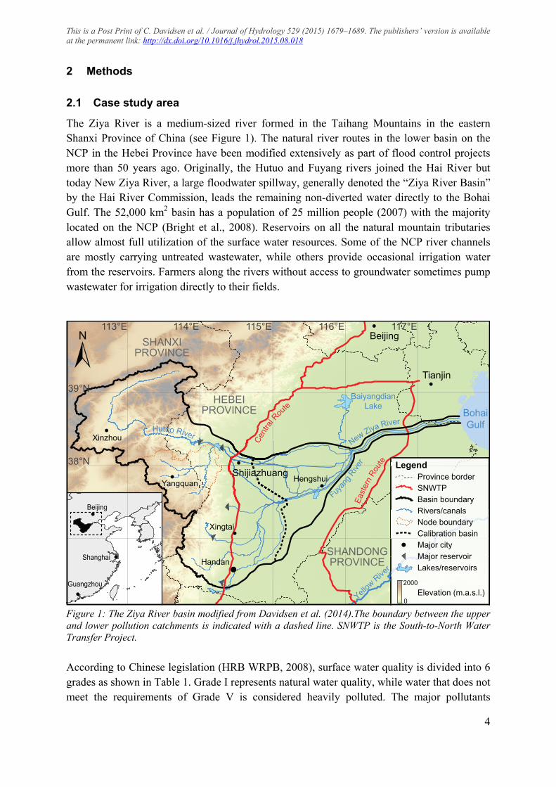
The Ziya River is a medium-sized river formed in the Taihang Mountains in the eastern Shanxi Province of China (see Figure 1). The natural river routes in the lower basin on the NCP in the Hebei Province have been modified extensively as part of flood control projects more than 50 years ago. Originally, the Hutuo and Fuyang rivers joined the Hai River but today New Ziya River, a large floodwater spillway, generally denoted the “Ziya River Basin” by the Hai River Commission, leads the remaining non-diverted water directly to the Bohai Gulf. The 52,000 km2 basin has a population of 25 million people (2007) with the majority located on the NCP (Bright et al., 2008). Reservoirs on all the natural mountain tributaries allow almost full utilization of the surface water resources. Some of the NCP river channels are mostly carrying untreated wastewater, while others provide occasional irrigation water from the reservoirs. Farmers along the rivers without access to groundwater sometimes pump wastewater for irrigation directly to their fields.
Figure 1: The Ziya River basin modified from Davidsen et al. (2014).The boundary between the upper and lower pollution catchments is indicated with a dashed line. SNWTP is the South-to-North Water Transfer Project.
According to Chinese legislation (HRB WRPB, 2008), surface water quality is divided into 6 grades as shown in Table 1. Grade I represents natural water quality, while water that does not meet the requirements of Grade V is considered heavily polluted. The major pollutants
BaiyangdianLake
SHANXIPROVINCE
HEBEIPROVINCE
SHANDONGPROVINCE
BohaiGulf
Yellow
Rive
r
New Ziya RiverHutuo River
Fuyan
g Rive
r±
Elevation (m.a.s.l.)2000
0
Legend
Basin boundaryRivers/canals
Major city
SNWTPProvince border
Lakes/reservoirs
Calibration basinNode boundary
Major reservoir
East
ern
Rout
e
Cent
ral R
oute
117°E116°E115°E114°E113°E
38°N
39°N
Xinzhou
Yangquan
Beijing
Shanghai
Guangzhou
Handan
Hengshui
Xingtai
Tianjin
C
Shijiazhuang
Beijing
!
!
!
!
!
!
!
!
!
!
!

This is a Post Print of C. Davidsen et al. / Journal of Hydrology 529 (2015) 1679–1689. The publishers’ version is available at the permanent link: http://dx.doi.org/10.1016/j.jhydrol.2015.08.018
5
include chemical oxygen demand (COD), BOD and ammonia (Ministry of Environmental Protection, 2010). In 2009, 42% of the river sections in the Hai River Basin failed to meet the Grade V standard (Ministry of Environmental Protection, 2010), which is also supported by our field observations. In the northern part of the Ziya River Basin, significant natural attenuation of pollutants is observed as the river flows from Xinzhou city through the Taihang Mountains and into the reservoirs located close to Shijiazhuang city. The main water quality challenges are therefore in the lower part of the catchment, and water quality in the upstream catchment is not considered in this study.
Table 1: Surface water quality classification in China (GB3838-2002, HRB WRPB, 2008) with selected water quality indicators shown. DO = dissolved oxygen, COD = Chemical Oxygen Demand and BOD5 = Biochemical Oxygen Demand over 5 days. All units are in g O2/m
3.
Quality DO ≥ COD ≤ BOD5 ≤
Grade I 90% of DOsat 15 3
Grade II 6 15 3
Grade III 5 20 4
Grade IV 3 30 6
Grade V 2 40 10
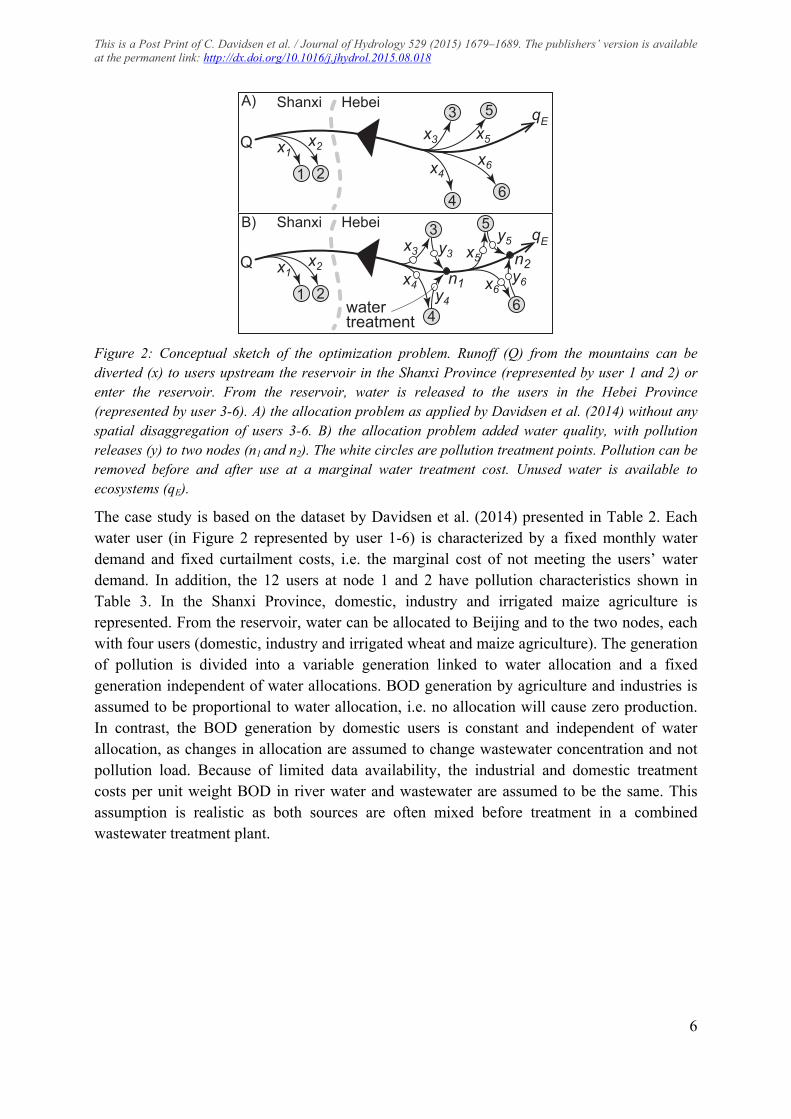
Simulation models can handle a high number of pollutants and are capable of simulating complex physical processes, whereas optimization models are, often computationally, limited to simpler representations of the real world problems (Harou et al., 2009). Davidsen et al. (2014) formalized the management problem as a simplified optimization as illustrated in Figure 2A with water users in three sectors irrigated agriculture, domestic and industries, upstream and downstream of a central reservoir. This central surface water reservoir is an aggregation of the five major reservoirs in the basin (see Davidsen et al., 2014) and it receives the combined runoff from the sub basins upstream these reservoirs. It is assumed that reservoir releases can be moved to any point downstream this central reservoir, an assumption which is realistic given high connectivity of the downstream rivers and channels. Runoff from both the Hutuo and Fuyang rivers is included in the aggregated reservoir model. The water values from the aggregated optimization model can be used with a much more detailed simulation model with multiple smaller reservoirs, within the suggested framework.
This is a Post Print of C. Davidsen et al. / Journal of Hydrology 529 (2015) 1679–1689. The publishers’ version is available at the permanent link: http://dx.doi.org/10.1016/j.jhydrol.2015.08.018
6
Figure 2: Conceptual sketch of the optimization problem. Runoff (Q) from the mountains can be diverted (x) to users upstream the reservoir in the Shanxi Province (represented by user 1 and 2) or enter the reservoir. From the reservoir, water is released to the users in the Hebei Province (represented by user 3-6). A) the allocation problem as applied by Davidsen et al. (2014) without any spatial disaggregation of users 3-6. B) the allocation problem added water quality, with pollution releases (y) to two nodes (n1 and n2). The white circles are pollution treatment points. Pollution can be removed before and after use at a marginal water treatment cost. Unused water is available to ecosystems (qE).
The case study is based on the dataset by Davidsen et al. (2014) presented in Table 2. Each water user (in Figure 2 represented by user 1-6) is characterized by a fixed monthly water demand and fixed curtailment costs, i.e. the marginal cost of not meeting the users’ water demand. In addition, the 12 users at node 1 and 2 have pollution characteristics shown in Table 3. In the Shanxi Province, domestic, industry and irrigated maize agriculture is represented. From the reservoir, water can be allocated to Beijing and to the two nodes, each with four users (domestic, industry and irrigated wheat and maize agriculture). The generation of pollution is divided into a variable generation linked to water allocation and a fixed generation independent of water allocations. BOD generation by agriculture and industries is assumed to be proportional to water allocation, i.e. no allocation will cause zero production. In contrast, the BOD generation by domestic users is constant and independent of water allocation, as changes in allocation are assumed to change wastewater concentration and not pollution load. Because of limited data availability, the industrial and domestic treatment costs per unit weight BOD in river water and wastewater are assumed to be the same. This assumption is realistic as both sources are often mixed before treatment in a combined wastewater treatment plant.
HebeiShanxiqE
qE
Q n2n1
y4y6
y3
x4 x6
x3x1 x2
water treatment
1 24
3 y5x5
5
6
HebeiShanxiA)
B)
Qx4
x6
x3x1 x2
1 2
4
3x5
5
6
This is a Post Print of C. Davidsen et al. / Journal of Hydrology 529 (2015) 1679–1689. The publishers’ version is available at the permanent link: http://dx.doi.org/10.1016/j.jhydrol.2015.08.018
7
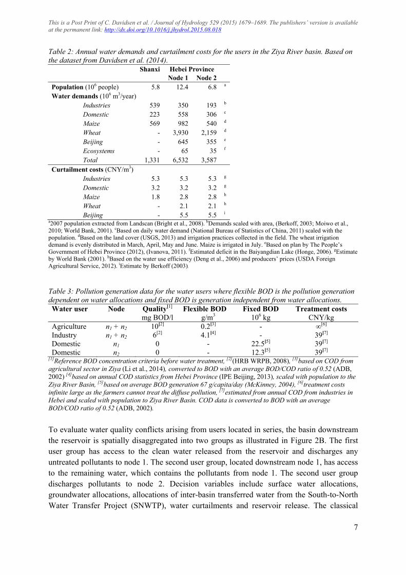
Table 2: Annual water demands and curtailment costs for the users in the Ziya River basin. Based on the dataset from Davidsen et al. (2014). Shanxi Hebei Province Node 1 Node 2 Population (106 people) 5.8 12.4 6.8 a Water demands (106 m3/year)
Industries 539 350 193 b Domestic 223 558 306 c Maize 569 982 540 d Wheat - 3,930 2,159 d Beijing - 645 355 e Ecosystems - 65 35 f
Total 1,331 6,532 3,587 Curtailment costs (CNY/m3)
Industries 5.3 5.3 5.3 g Domestic 3.2 3.2 3.2 g Maize 1.8 2.8 2.8 h Wheat - 2.1 2.1 h
Beijing - 5.5 5.5 i a2007 population extracted from Landscan (Bright et al., 2008). bDemands scaled with area, (Berkoff, 2003; Moiwo et al., 2010; World Bank, 2001). cBased on daily water demand (National Bureau of Statistics of China, 2011) scaled with the population. dBased on the land cover (USGS, 2013) and irrigation practices collected in the field. The wheat irrigation demand is evenly distributed in March, April, May and June. Maize is irrigated in July. eBased on plan by The People’s Government of Hebei Province (2012), (Ivanova, 2011). fEstimated deficit in the Baiyangdian Lake (Honge, 2006). gEstimate by World Bank (2001). hBased on the water use efficiency (Deng et al., 2006) and producers’ prices (USDA Foreign Agricultural Service, 2012). iEstimate by Berkoff (2003).
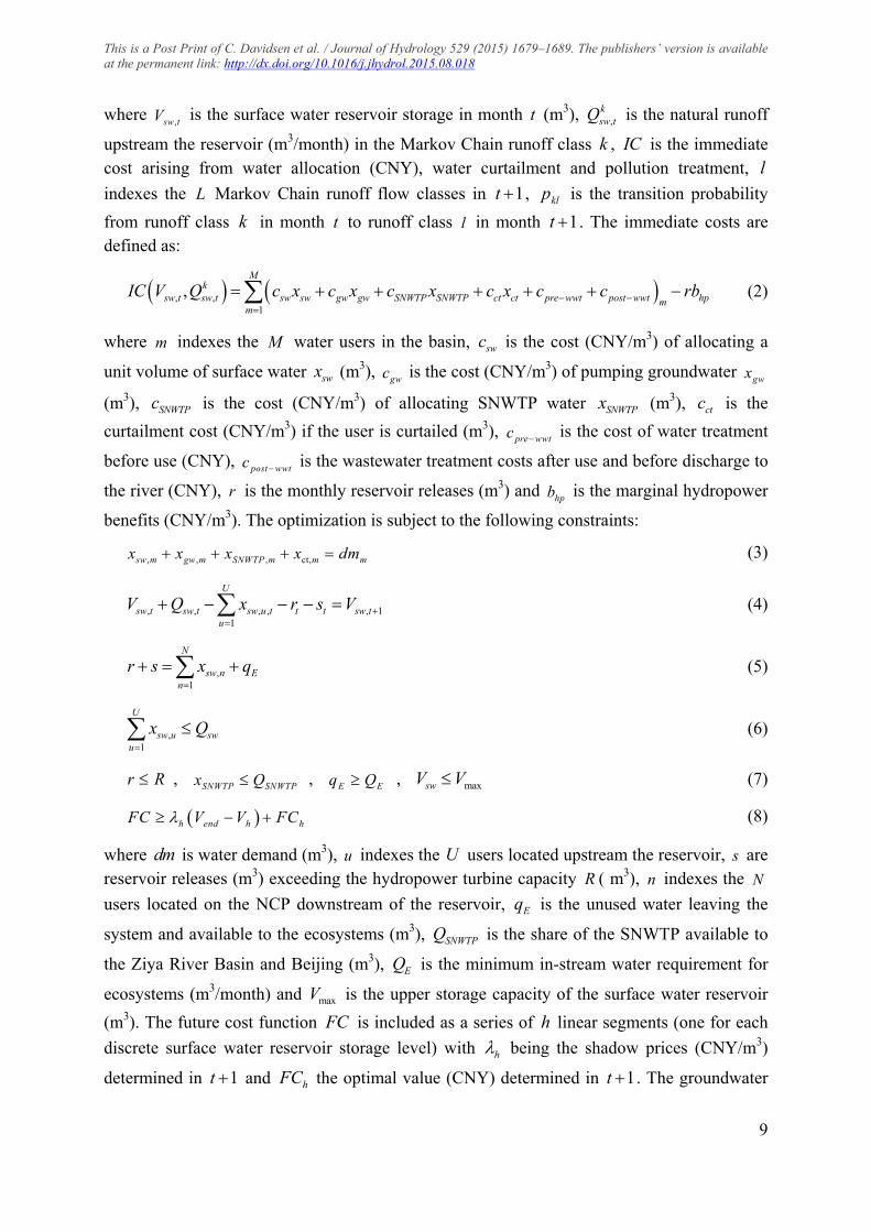
Table 3: Pollution generation data for the water users where flexible BOD is the pollution generation dependent on water allocations and fixed BOD is generation independent from water allocations. Water user Node Quality[1] Flexible BOD Fixed BOD Treatment costs mg BOD/l g/m3 106 kg CNY/kg Agriculture n1 + n2 10[2] 0.2[3] - ∞[6] Industry n1 + n2 6[2] 4.1[4] - 39[7] Domestic n1 0 - 22.5[5] 39[7] Domestic n2 0 - 12.3[5] 39[7]
[1]Reference BOD concentration criteria before water treatment, [2](HRB WRPB, 2008), [3]based on COD from agricultural sector in Ziya (Li et al., 2014), converted to BOD with an average BOD/COD ratio of 0.52 (ADB, 2002) [4]based on annual COD statistics from Hebei Province (IPE Beijing, 2013), scaled with population to the Ziya River Basin, [5]based on average BOD generation 67 g/capita/day (McKinney, 2004), [6]treatment costs infinite large as the farmers cannot treat the diffuse pollution, [7]estimated from annual COD from industries in Hebei and scaled with population to Ziya River Basin. COD data is converted to BOD with an average BOD/COD ratio of 0.52 (ADB, 2002).
To evaluate water quality conflicts arising from users located in series, the basin downstream the reservoir is spatially disaggregated into two groups as illustrated in Figure 2B. The first user group has access to the clean water released from the reservoir and discharges any untreated pollutants to node 1. The second user group, located downstream node 1, has access to the remaining water, which contains the pollutants from node 1. The second user group discharges pollutants to node 2. Decision variables include surface water allocations, groundwater allocations, allocations of inter-basin transferred water from the South-to-North Water Transfer Project (SNWTP), water curtailments and reservoir release. The classical

This is a Post Print of C. Davidsen et al. / Journal of Hydrology 529 (2015) 1679–1689. The publishers’ version is available at the permanent link: http://dx.doi.org/10.1016/j.jhydrol.2015.08.018
8
water allocation problem is extended to include optimal pollution discharge and water treatment, while complying with water quality requirements in the river. In Figure 2B, the additional water quality decisions (removal of pollutants from the intake surface water before use, removal of generated pollutants and pollution concentration at the two nodes) are indicated. Unused water flows to the Bohai Gulf or is utilized for ecosystem services. In Figure 1, the assumed boundary between the upstream and downstream areas is indicated. To compute the industrial and domestic water demands, total demands are scaled with the share of total 2007 population (Bright et al., 2008), while the irrigation water demands are scaled by the share of total area.
2.2 Optimization model formulation
In our approach, we assume that the combined storage capacity of the surface water reservoirs can be operated fully flexibly and without consideration of existing regulations and policies. The natural runoff was estimated by Davidsen et al. (2014) with a rainfall-runoff model based on the Budyko framework (Budyko, 1958; Zhang et al., 2008). The hydrological model was set up for a close-to-natural sub-catchment in the mountains and calibrated to measured runoff at the Pingshan station (Number 30912428) (MWR. Bureau of Hydrology, 2011). The calibrated model was applied to all sub-catchments located upstream of the reservoirs. The resulting 51 years of daily runoff from 1958 to 2008 was aggregated to monthly time steps and normalized. A 3-state Markov Chain, which describes the runoff serial correlation between three flow classes defined as dry (0 – 20th percentile), normal (20th – 80th percentile), and wet (80th – 100th percentile) was established. The Markov Chain was validated to ensure second-order stationarity (Loucks and van Beek, 2005). A shift in the regional precipitation pattern previously reported in the literature is observed in the precipitation time series (Cao et al., 2013; Chen, 2010; Sun et al., 2010). The shift is assumed to occur in 1980 with stationary climate before and after this year.
The simplified management problem with water quality (see Figure 2B) is formalized as a stochastic dynamic program similar to the model by Davidsen et al. (2014), with stochastic unknown future runoff. We applied the water value method, a variant of SDP, to identify a long-term optimal water management strategy for the basin (Pereira and Pinto, 1991; Stage and Larsson, 1961; Stedinger et al., 1984). The SDP proceeds recursively backward in time in monthly time steps (stages) and, for each stage, loops through all possible combinations of states, here the Markov Chain flow classes and discrete surface water reservoir storage levels. Thereby, all possible management decisions are evaluated, as the SDP produces the decision rules, assuming stochastic runoff. For each combination of system states, a sub optimization problem, which minimizes the sum of the immediate and expected future costs, is solved. The
optimal value function ,*
, ,t sw tksw tF V Q is based on the classical Bellman formulation:
*, , 1 , 1
*
1, , , 1, min , ,t sw t sw t
Lk k lsw t sw t tkl sw t sw t
l
F V Q IC V Q p F V Q
(1)
This is a Post Print of C. Davidsen et al. / Journal of Hydrology 529 (2015) 1679–1689. The publishers’ version is available at the permanent link: http://dx.doi.org/10.1016/j.jhydrol.2015.08.018
9
where ,sw tV is the surface water reservoir storage in month t (m3), ,ksw tQ is the natural runoff
upstream the reservoir (m3/month) in the Markov Chain runoff class k , IC is the immediate cost arising from water allocation (CNY), water curtailment and pollution treatment, l
indexes the L Markov Chain runoff flow classes in 1t , klp is the transition probability
from runoff class k in month t to runoff class l in month 1t . The immediate costs are defined as:
, ,1
,M
ksw t SNWTP SNWTP ct csw t sw sw gw gw pre wwt post wwt ht
mpm
IC V Q c x c x c x c x c c rb
(2)
where m indexes the M water users in the basin, swc is the cost (CNY/m3) of allocating a
unit volume of surface water swx (m3), gwc is the cost (CNY/m3) of pumping groundwater gwx
(m3), SNWTPc is the cost (CNY/m3) of allocating SNWTP water SNWTPx (m3), ctc is the
curtailment cost (CNY/m3) if the user is curtailed (m3), pre wwtc is the cost of water treatment
before use (CNY), post wwtc is the wastewater treatment costs after use and before discharge to
the river (CNY), r is the monthly reservoir releases (m3) and hpb is the marginal hydropower
benefits (CNY/m3). The optimization is subject to the following constraints:
, , , ct,sw m gw m SNWTP m m mdx x x mx (3)
, , , , 11
,
U
usw t sw t sw u t t t sw tV Q rx s V
(4)
,1
sw nn
E
N
s qr x
(5)
1
,w u su
s w
U
x Q
(6)
r R , SNWTP SNWTPx Q , E Eq Q , maxswV V (7)
h end h hV FF V CC (8)
where dm is water demand (m3), u indexes the U users located upstream the reservoir, s are reservoir releases (m3) exceeding the hydropower turbine capacity R ( m3), n indexes the N
users located on the NCP downstream of the reservoir, Eq is the unused water leaving the
system and available to the ecosystems (m3), SNWTPQ is the share of the SNWTP available to
the Ziya River Basin and Beijing (m3), EQ is the minimum in-stream water requirement for
ecosystems (m3/month) and maxV is the upper storage capacity of the surface water reservoir
(m3). The future cost function FC is included as a series of h linear segments (one for each
discrete surface water reservoir storage level) with h being the shadow prices (CNY/m3)
determined in 1t and hFC the optimal value (CNY) determined in 1t . The groundwater

This is a Post Print of C. Davidsen et al. / Journal of Hydrology 529 (2015) 1679–1689. The publishers’ version is available at the permanent link: http://dx.doi.org/10.1016/j.jhydrol.2015.08.018
10
resource is available for unrestricted pumping at a given fixed use cost gwc (CNY/m3),
adopted from Davidsen et al. (n.d.).
Eq. 3 is the demand fulfillment constraint, i.e. the sum of allocations and water curtailment must equal the water demand. Eq. 4 is the water balance equation for the surface water reservoir, while Eq. 5 is the water balance for the reservoir releases. Water users upstream of the reservoir have no access to surface water storage and are therefore limited to the monthly runoff as shown in Eq. 6.
Each stage of the backward moving SDP is fully parallelized as the states within a single stage are independent. In the initial stage of the backward-in-time recursive loop, the future costs are set to zero. With no future costs, the optimal strategy is to empty the reservoir. As the SDP moves backward in time, the future costs become increasingly important and the benefits of emptying the reservoir in t are traded off against increased costs of low storage in
1t and onwards. The yearly backward recursion is repeated until the immediate and future costs in t are no longer affected by the end conditions (zero future costs). At this point, the inter-annual difference in the shadow prices, becomes zero and the model has reached equilibrium.
The equilibrium water value tables are suitable for decision support in a water pricing scheme and application in real-time water management, assuming stochastic future runoff, as demonstrated in a simulation run. The simulation run finds the series of monthly water allocations, water curtailments and water treatment decisions, which minimizes the total costs (sum of water curtailment costs, water treatment costs, water allocation costs and hydropower benefits) over a given planning period. From a given starting point with known runoff, month and reservoir storage level, the present flow class is determined as dry, normal or wet. The corresponding equilibrium water values and future costs are used as the expected future cost function as presented in Eq. 8. These future costs are traded off against the immediate costs, which yields the expected present optimal reservoir release and allocation policy, similarly to the backward moving SDP algorithm. Moving to the next month, the reservoir storage level is known from the previous reservoir inflow and releases. This simulation model is run through the 51 years of simulated runoff. Additionally, a perfect foresight benchmark based on dynamic programming (DP) is run. In this setup, the inflows occurring over the entire planning period are assumed to be known a priori.
This is a Post Print of C. Davidsen et al. / Journal of Hydrology 529 (2015) 1679–1689. The publishers’ version is available at the permanent link: http://dx.doi.org/10.1016/j.jhydrol.2015.08.018
11
2.3 Water quality constraints
The optimization model is subject to water quality constraints. We use BOD to demonstrate the water quality capabilities of the method, but the model is able to handle a variety of other pollutants as explained in the discussion section. In contrast to other pollutants, the main problem of BOD is not the direct toxic effect but the oxygen depletion resulting from BOD load. The water quality constraints are therefore set as lower bounds on the dissolved oxygen concentration DO at any point in the river.
The objective function includes water treatment costs. The monthly total pollution reduction
costs ( wwttc ) for each of the downstream users are defined as the sum of the pre-usage
treatments ( pre wwtc ) for water exceeding user specific reference water quality and post-usage
treatment costs ( post wwtc ):
wwt pre wwt post wwttc c c (9)
with
,
0,
wt refsw refpre wwt
ref
C Cx C C cc
C C
(10)
,
0,post wwt
wwtx y c x yc
x y
(11)
where C is the pollutant concentration at the intake point (g BOD/m3 in river), refC is the
maximum concentration of pollutant given by the user-specific reference water quality target
(see Table 3) at which pre-usage treatment is initiated (g BOD/m3 in the river), wtc is the
marginal water treatment costs of intake water (CNY/g BOD), is the BOD generation dependent on water allocations (g BOD/m3 allocated) (see Table 3), x is the total allocated water to the user (m3/month), is the fixed BOD generation independent of water allocations
(g BOD/month), y is the non-treated pollution release to the river (g BOD/month) and wwtc is
the waste water treatment costs of reducing the pollution load of the return flow (CNY/g BOD).
The pollution pre-treatment is governed by the surface water allocation decision variable, the
pollutant concentration in the river and two constants ( refC and wtc ). For node 1, the pollutant
concentration is a function of the reservoir release, the surface water allocations to and the pollution releases from the users located at node 1:
1 0
, ,
...
...j J
sw j sw J
y yC C
r x x
(12)
where 1C is the concentration at node 1 (g BOD/m3), 0C is the pollutant concentration in the
reservoir release (g BOD/m3) and j indexes the J users located at node 1. From this equation

This is a Post Print of C. Davidsen et al. / Journal of Hydrology 529 (2015) 1679–1689. The publishers’ version is available at the permanent link: http://dx.doi.org/10.1016/j.jhydrol.2015.08.018
12
it is evident that the pollutant concentration depends nonlinearly on multiple decision
variables ( y , swx , r ).
The downstream management problem is spatially disaggregated as sketched in Figure 2B, with two groups of water users located in series with a distance dx (m) between them. If the flow velocity v (m/d) is assumed constant, the elapsed time between the two nodes is also constant ( /t dx v ). The BOD removal is assumed to follow first order decay:
1
dBODk
dtBOD (13)
with the solution:
0 1expBOD t BOD k t (14)
where 1k is the deoxygenation rate (d-1). The remaining BOD at node 2 is found from the
travel time of the water between the two nodes:
1
,
2
,
1
, ,
...exp
... ...sw j sw J sw z s
Z
w Z
zy yC C k t
r x x x x
(15)
where z indexes the Z users located at node 2. The concentration at node 2 is, just like node 1, a non-linear expression of multiple decision variables. The concentration depends both on the upstream decisions and the allocations and post-use treatments at node 2.
The post-usage treatment cost in Eq. 11 is a linear expression of the decision variables. The Streeter-Phelps equation estimates the DO concentration in the river, assuming perfect mixing in the river (Streeter and Phelps, 1958):
1 2 210
2 1
0 k t k t k tk BODD e e D e
k k
(16)
where D is the oxygen saturation deficit (g/m3) ( satDO DO ), 2k is the reaeration rate (d-1),
0BOD is the initial oxygen demand of the organic matter in the water (g/m3), t is the elapsed
time (d) and 0D is the initial oxygen saturation deficit (g/m3). The dissolved oxygen
concentration DO (g/m3) is derived from the saturated oxygen concentration satDO (g/m3):
satD DO DO (17)
The dissolved oxygen concentration is a function of the elapsed time and decreases until the
critical time ct (d) at which the deficit reaches its maximum (i.e. the dissolved oxygen is at
minimum). In a river water quality perspective, location and value of this critical dissolved oxygen concentration are of interest. The water quality constraint should be expressed in terms of the critical concentration, i.e. at no point downstream in the river does the dissolved oxygen concentrations fall below a given constraint. The critical time is found by differentiating Eq. 16 with respect to time and setting this equal to zero:
This is a Post Print of C. Davidsen et al. / Journal of Hydrology 529 (2015) 1679–1689. The publishers’ version is available at the permanent link: http://dx.doi.org/10.1016/j.jhydrol.2015.08.018
13
0 2 12
2 1 1 0 1
1ln 1c
D k kkt
k k k BOD k
(18)
Insertion of the critical time in Eq. 16 yields an expression of the maximum dissolved oxygen
deficit critD (g/m3). The minimum dissolved oxygen concentration, minDO (g/m3) downstream
node 1 is found by inserting maxD and the given initial conditions for satDO , 0D , 1k , 2k and
aL in Eq. 17. Similarly, the Streeter-Phelps equation is used to compute minDO downstream
node 2. Here the remaining BOD and DO are found by inserting the elapsed time between the
two nodes in Eq. 14 and 16 and 0D and 0BOD are the calculated values at the end of the
upstream section. With the BOD concentrations at node 1 and 2 as the only inputs, the
resulting minDO downstream both nodes are found.
The saturated oxygen concentration along with the reaeration and deoxygenation processes is highly temperature dependent (Schnoor, 1996). The optimization runs in monthly time steps
and the temperature in the basin varies greatly throughout the year. 1k and 2k were therefore
temperature corrected (Schnoor, 1996):
(T 20),20i ik k (19)
where ,20ik is the reaeration or the BOD assimilation rate at 20°C, with 1,20k estimated to 0.3
d-1 and 2,20k estimated to 0.6 d-1, T is the actual stream temperature, and is a constant. For
1k , has the value 1.047, and for 2k the value 1.024 (Schnoor, 1996). The saturated
dissolved oxygen concentration is estimated with Weiss baseline DO concentration at zero salinity and one atmosphere (U.S. Geological Survey, 2013; Weiss, 1970).
The daily minimum and maximum air temperatures reported by the China Meteorological Administration (2009) is averaged to monthly levels. The average water temperature is assumed to be equal to the average air temperature. In Table 4 the average monthly air temperatures, the corresponding oxygen solubility and the temperature corrected deoxygenation and reaeration rates are presented.

This is a Post Print of C. Davidsen et al. / Journal of Hydrology 529 (2015) 1679–1689. The publishers’ version is available at the permanent link: http://dx.doi.org/10.1016/j.jhydrol.2015.08.018
14
Table 4: Mean air temperature, the oxygen solubility at saturation and the temperature corrected BOD assimilation and reaeration rates. *For January, a water temperature of zero degrees Celsius is used.
Month Mean T satDO 1k 2k°C g/m3 d-1 d-1
Jan -2.1* 14.6 0.11 0.36Feb 1.1 14.2 0.13 0.38Mar 7.7 11.9 0.17 0.45Apr 15.3 10.0 0.24 0.54May 21.2 8.9 0.32 0.62Jun 26.0 8.1 0.40 0.69Jul 27.2 7.9 0.42 0.71
Aug 25.8 8.1 0.39 0.69Sep 21.2 8.9 0.32 0.62Oct 14.7 10.1 0.24 0.53Nov 6.3 12.4 0.16 0.43Dec 0.0 14.6 0.12 0.37
2.4 Solving the nonlinear sub problems
If the optimization problem is strictly linear and convex, linear programming is a highly efficient approach to solve the high number of optimization sub-problems arising within the SDP framework. In this study, the sub-problems are non-linear because of the water quality constraints and an alternative to LP is therefore needed. Efficient genetic algorithms (GA, see e.g. Goldberg, 1989; Reeves, 1997) have been used widely to find the global optimum in complex nonlinear optimization problems. In water resources management, GAs have been applied for a variety of nonlinear optimization problems such as, for example, coupled groundwater-surface water management problems, hydropower production and reservoir water quality problems (Cai et al., 2001; Davidsen et al., n.d.; Kerachian and Karamouz, 2007; Nicklow et al., 2010). A GA searches for the global optimal solution with a search approach inspired by natural evolution. Using a GA with in our case more than 70 decision variables is expected to be computationally infeasible within the SDP framework. Cai et al. (2001) developed a hybrid GA-LP implementation to solve a nonlinear surface water management problem. In this approach, the complicating decision variables, which cause the nonlinearity, are “outsourced” to the GA. With these complicating values fixed, the remaining optimization problem becomes strictly linear and solvable with LP. As demonstrated in Eq. 12 and 15, the BOD concentrations in node 1 and 2 both depend on multiple decision
variables, and fixing 1C and 2C reduces the remaining decisions to an LP. The GA uses the
fast LP as fitness measure, as it iteratively searches for the optimal solution in each discrete combination of system states.
The optimization model is developed in MATLAB and uses the standard GA function ga (MathWorks Inc., 2013). The options for ga are selected through multiple test runs and include, besides the default options, a population size of 30, constraint and function tolerances of 10-9, elite count of 5 and a migration interval of 1. Finally, a random uniform population is generated within the feasible decision space and supplied as the initial population to ga. The

This is a Post Print of C. Davidsen et al. / Journal of Hydrology 529 (2015) 1679–1689. The publishers’ version is available at the permanent link: http://dx.doi.org/10.1016/j.jhydrol.2015.08.018
15
default MATLAB function linprog can be used to solve the LP, but in this study the computationally faster commercial solver cplexlp by IBM is used (IBM, 2013). Each stage is fully parallelized as all storage levels and the Markov Chain flow classes are fully independent. With 30 discrete reservoir storage levels and 3 flow classes, each optimization year requires 25 minutes on 18 2.8 GHz cores in a high performance computer (HPC) environment. With a need of estimated 10 optimization years to reach equilibrium, the total optimization time becomes around 4 hours per climate period per scenario.
The SDP model loops through flow classes and reservoir storage levels backward in time. A flow chart of the algorithm design is presented in Figure 3. Initially, the input data are assigned, including an initial population of feasible samples. Next, an LP with the BOD concentration at each node given as input variables is used to find the minimum summed costs of immediate management and future costs. In MATLAB the LP is supplied as a fitness function to the GA, with the node concentrations as the two decisions. As the GA iteratively approaches the optimal solution, new mutations and crossovers of parents are constrained by the minimum DO concentration, computed with the Streeter-Phelps equation. The Streeter-Phelps equation is supplied as a nonlinear constraint to the GA.
Figure 3: Flow chart of the SDP model and the simulation phase.
Classification of historic runoff into flow classes and extraction of
transition probabilities
Set future costs of t equal to zero
Generation of future cost function and initial population
DO constraint
Optimal solutions found to all flow classes and reservoir storage levels?
Water values at equilibrium?
Simulation phase
Computation of fitness values
Selection of best parents
Mutation and crossover
Convergence to optimal solution?
Select a reservoir storage level and flow class
Move one stage back in time
Yes
Yes
Yes
No
No
No
LPGA
Reservoir storage level in t-1
Generation of future cost function from equilibrium water values in
t +1 and initial population DO constraint
End of planning period reached?
Simulation phase complete
Computation of fitness values
Selection of best parents
Mutation and crossover
Convergence to optimal solution?
Classification of present runoff
Move one stage forward in time
Yes
YesNo
No
LPGA

This is a Post Print of C. Davidsen et al. / Journal of Hydrology 529 (2015) 1679–1689. The publishers’ version is available at the permanent link: http://dx.doi.org/10.1016/j.jhydrol.2015.08.018
16
2.5 Scenario runs and local sensitivity analysis
Several scenarios were simulated to demonstrate the potential use of the model in decision support. By default, a monthly minimum in-stream flow to the ecosystem is set to 5% of the natural runoff. Davidsen et al. (n.d.) found that the long-term sustainable groundwater pumping costs in the Ziya River Basin can be assumed constant. At steady state, the groundwater cost is constant at approximately 2.2 CNY/m3. If the groundwater table is below equilibrium, the groundwater cost is higher. The groundwater cost is set at a constant value of 2.5 CNY/m3 in this study, to stimulate recovery of the currently over-pumped groundwater aquifer.
The first scenario is a baseline run that does not consider water quality constraints,. Five additional scenarios require compliance with the five water quality grades presented in Table 1. In the No Treatment (NT) scenario, water cannot be treated, i.e. water quality constraints must be satisfied by dilution and curtailment only. A final scenario with water quality constraint set to grade III and a minimum in-stream flow constraint at 20% of the natural runoff is run to estimate the costs of obtaining close-to-natural conditions in the river.
Because of the high computational load, a Monte Carlo uncertainty analysis as applied by Davidsen et al. (2014) is infeasible. Instead, a local sensitivity analysis of the total cost was conducted. Five uncertain parameters were identified in the input data; water demands, water curtailment costs, wastewater treatment costs, BOD generation and river flow velocity. Each parameter was increased by 10%, and the resulting change in the total costs used as a measure of sensitivity.
3 Results and discussion
A sample of the equilibrium water value tables generated in the 7 scenario runs are presented in Figure 4. These water values show the value of storing a marginal volume of water in the reservoir for later use. The water values are lowest in the rainy season (June-August) when water values are comparable to hydropower benefits at 0.036 CNY/m3. In the dry winter and spring months water values are typically around 2.2 CNY/m3 for storage above 1/3 of the reservoir capacity (reflects curtailment of wheat agriculture) and 2.5 CNY/m3 below 1/3 storage (shift to groundwater pumping). As the water quality is improved, the marginal values of storing water increases particularly in the wet months.
This is a Post Print of C. Davidsen et al. / Journal of Hydrology 529 (2015) 1679–1689. The publishers’ version is available at the permanent link: http://dx.doi.org/10.1016/j.jhydrol.2015.08.018
17
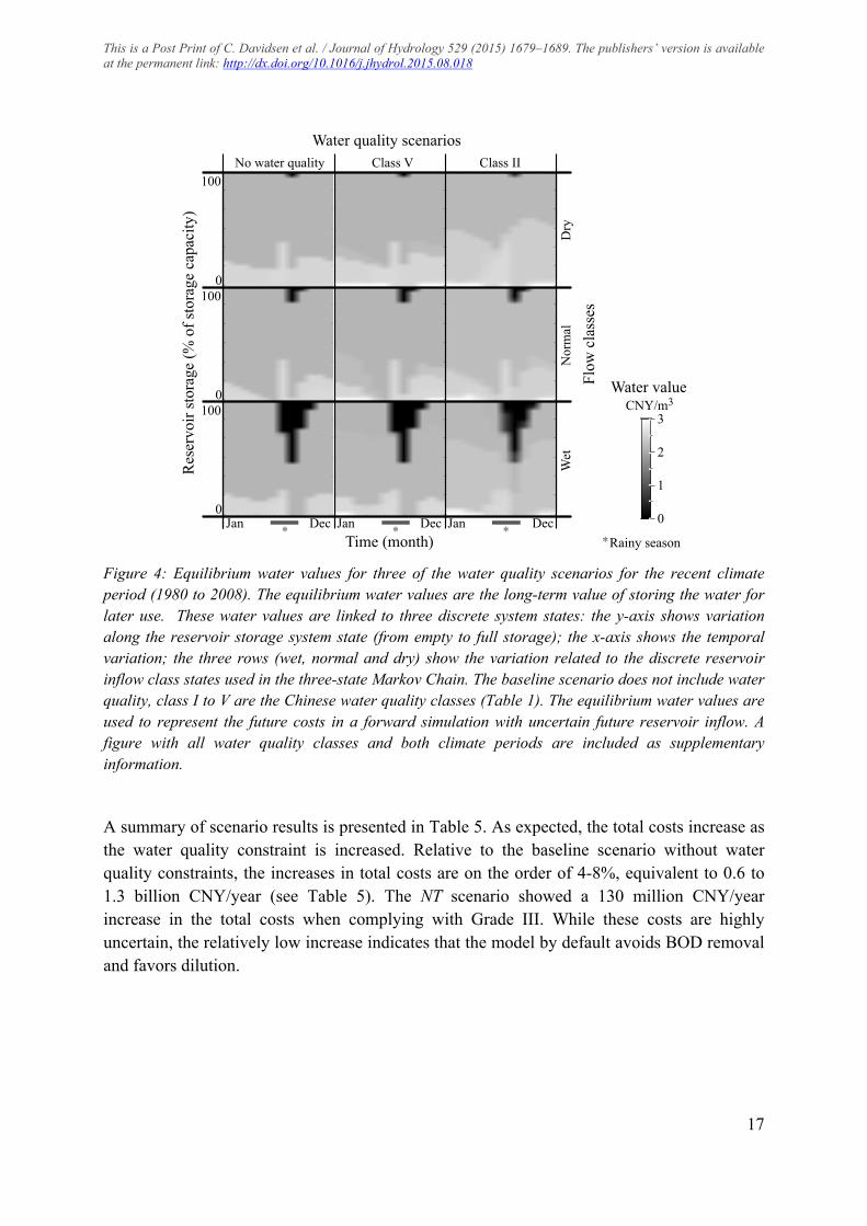
Figure 4: Equilibrium water values for three of the water quality scenarios for the recent climate period (1980 to 2008). The equilibrium water values are the long-term value of storing the water for later use. These water values are linked to three discrete system states: the y-axis shows variation along the reservoir storage system state (from empty to full storage); the x-axis shows the temporal variation; the three rows (wet, normal and dry) show the variation related to the discrete reservoir inflow class states used in the three-state Markov Chain. The baseline scenario does not include water quality, class I to V are the Chinese water quality classes (Table 1). The equilibrium water values are used to represent the future costs in a forward simulation with uncertain future reservoir inflow. A figure with all water quality classes and both climate periods are included as supplementary information.
A summary of scenario results is presented in Table 5. As expected, the total costs increase as the water quality constraint is increased. Relative to the baseline scenario without water quality constraints, the increases in total costs are on the order of 4-8%, equivalent to 0.6 to 1.3 billion CNY/year (see Table 5). The NT scenario showed a 130 million CNY/year increase in the total costs when complying with Grade III. While these costs are highly uncertain, the relatively low increase indicates that the model by default avoids BOD removal and favors dilution.
��
���
���
���
���
���
���
��
��
���
�
���� ��
0
100
0
100
0
100
No water quality Class V Class II
Dry
Nor
mal
Water value
Res
ervo
ir st
orag
e (%
of s
tora
ge c
apac
ity)
Flow
cla
sses
Water quality scenarios
Time (month)
CNY/m33
2
1
0Jan Dec Jan Dec Jan DecRainy season
***
Wet
�
*

This is a Post Print of C. Davidsen et al. / Journal of Hydrology 529 (2015) 1679–1689. The publishers’ version is available at the permanent link: http://dx.doi.org/10.1016/j.jhydrol.2015.08.018
18
Table 5: Total costs for all scenarios where TC is the average total costs over the 51 year planning period, DP is the simulation with perfect foresight (dynamic programming), E20 is minimum ecosystem releases set to 20% of natural runoff, NT is the simulation with water quality constrains but no wastewater treatment facilities. The last five rows are the sensitivity with 10% increased dm (water demands), ct (curtailment costs), cwt (marginal costs of wastewater treatment), pg (pollution generation) and v (flow velocity in the river).
Quality Run DO TC SDP TC DP Sensitivity mg/l 109 CNY/year 109 CNY/year % change
Baseline E5 - 15.6 15.4 Grade V E5 ≥ 2 16.2 16.0 Grade IV E5 ≥ 3 16.3 16.0 Grade III E5 ≥ 5 16.4 16.1 Grade II E5 ≥ 6 16.4 16.2 Grade I E5 ≥0.9DOsat 16.9 16.7 Grade III E20 ≥ 5 17.0 - Grade III NT ≥ 5 16.5 - Grade III dm ≥ 5 18.8 - 15.3 Grade III ct ≥ 5 17.6 - 7.4 Grade III cwt ≥ 5 16.4 - 0.1 Grade III pg ≥ 5 16.5 - 0.5 Grade III v ≥ 5 16.4 - 0.1
The simple local sensitivity analysis shows that the total costs are highly sensitive to water demands. A 10% increase of the water demands leads to more severe water scarcity and increases the total costs by 15.3%. Demands of the most expensive users remain fulfilled with groundwater (at a cost of 2.5 CNY/m3) while cheaper water uses will be more curtailed. The water curtailment costs are less sensitive; a 10% increase in curtailment costs increases the total costs by 7.4%. Here, the demands of the most expensive water uses will remain fulfilled with groundwater (no additional costs) while the cost of curtailing the cheaper water uses will increase. The average marginal value per m3 of water demand supplied or curtailed is 1.44 CNY/m3. With all water already allocated, a 10% increase in the water demand causes more curtailments and more groundwater pumping both at marginal costs higher than 2 CNY/m3. Moreover, BOD load is proportional to water allocation. Increased water treatment, curtailment or dilution is therefore required. In comparison, a 10% increase in the curtailment costs affects only the users that are curtailed. The total costs show almost no sensitivity towards increases of the wastewater treatment costs, pollution generation and river flow velocity.
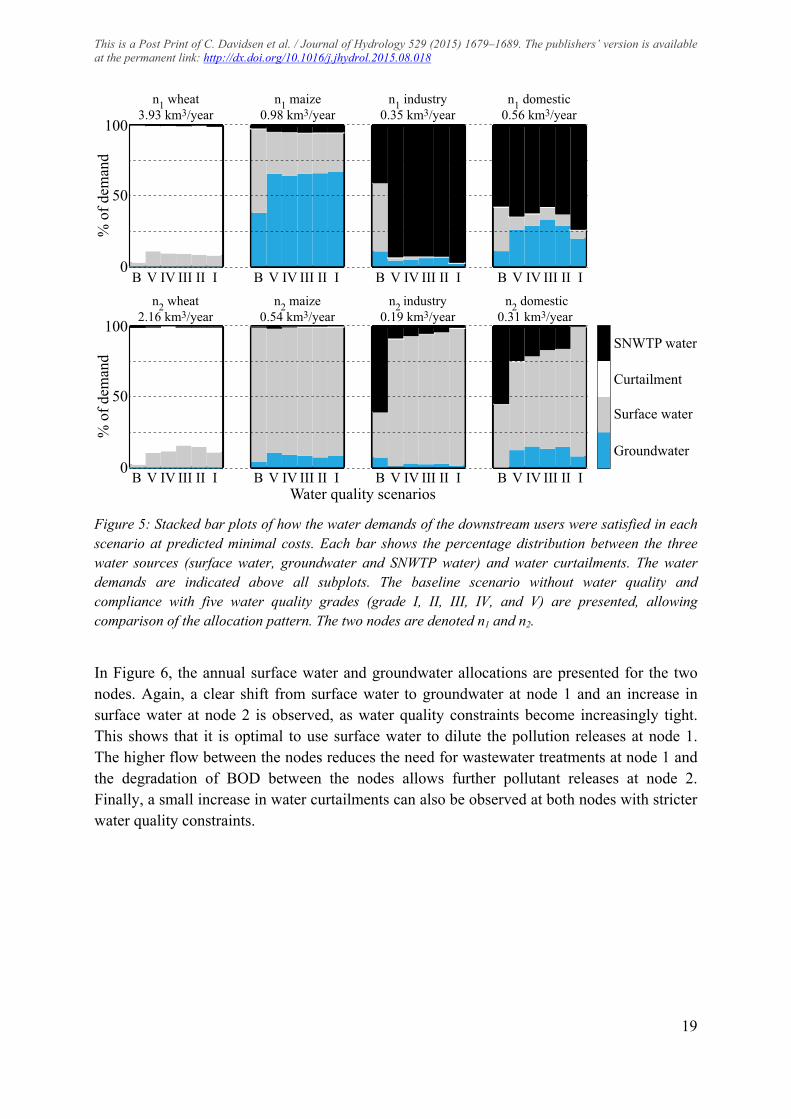
In Figure 5, the aggregated water allocation patterns are presented for the individual users at the two downstream nodes across the water quality scenarios. Each bar shows the portion of the water demand that is fulfilled using the different water sources. With tighter water quality requirements, more groundwater is allocated to the users at node 1, while the users at node 2 receive an increasing share of the surface water. Compared to the baseline scenario without water quality, wheat agriculture receives more water in all the water quality scenarios.
This is a Post Print of C. Davidsen et al. / Journal of Hydrology 529 (2015) 1679–1689. The publishers’ version is available at the permanent link: http://dx.doi.org/10.1016/j.jhydrol.2015.08.018
19
Figure 5: Stacked bar plots of how the water demands of the downstream users were satisfied in each scenario at predicted minimal costs. Each bar shows the percentage distribution between the three water sources (surface water, groundwater and SNWTP water) and water curtailments. The water demands are indicated above all subplots. The baseline scenario without water quality and compliance with five water quality grades (grade I, II, III, IV, and V) are presented, allowing comparison of the allocation pattern. The two nodes are denoted n1 and n2.
In Figure 6, the annual surface water and groundwater allocations are presented for the two nodes. Again, a clear shift from surface water to groundwater at node 1 and an increase in surface water at node 2 is observed, as water quality constraints become increasingly tight. This shows that it is optimal to use surface water to dilute the pollution releases at node 1. The higher flow between the nodes reduces the need for wastewater treatments at node 1 and the degradation of BOD between the nodes allows further pollutant releases at node 2. Finally, a small increase in water curtailments can also be observed at both nodes with stricter water quality constraints.
B V IV III II I0
0
0
B V IV III II I0
50
100
B V IV III II I0
50
100
B V IV III II I0
50
100
0
0
0
0
50
100
0
50
100
0
50
100
Curtailment
SNWTP water
Surface water
Groundwater
% o
f dem
and
Water quality scenarios
% o
f dem
and
n1 wheat3.93 km3/year
n1 maize0.98 km3/year
n1 industry0.35 km3/year
n1 domestic0.56 km3/year
% o
f dem
and
100
50
0
% o
f dem
and
% o
f dem
and
100
50
0B V IV III II I B V IV III II I B V IV III II I B V IV III II I
B V IV III II I B V IV III II I B V IV III II I B V IV III II In2 wheat
2.16 km3/yearn2 maize
0.54 km3/yearn2 industry
0.19 km3/yearn2 domestic
0.31 km3/year

This is a Post Print of C. Davidsen et al. / Journal of Hydrology 529 (2015) 1679–1689. The publishers’ version is available at the permanent link: http://dx.doi.org/10.1016/j.jhydrol.2015.08.018
20
Figure 6: Annual allocation to and curtailment of the users at node 1 and node 2 for the baseline scenario without water quality (B) and the five water quality grades (grade I, II, III, IV, and V). Water reserved for ecosystems is shown with the node 2 data. With higher DOmin constraints, the surface water allocations are shifted towards the users at node 2 to utilize the water for dilution. This surface water is replaced with groundwater and SNWTP water at node 1. A small increase in water curtailments can also be observed at the stricter water quality scenarios.
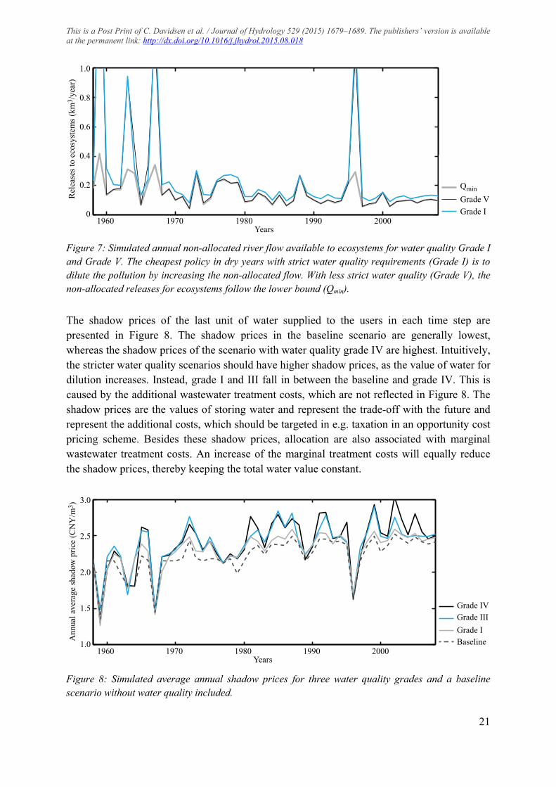
The non-allocated in-stream flow available to ecosystems is presented in Figure 7 for water quality grade I and grade V. In these scenarios, the minimum flow constraint is set to 5% of the natural runoff, indicated by the grey line. Apart from four flooding events, latest in 1996, releases are exactly 5% of the natural runoff, when complying with grade V. The minimum flow constraint is therefore binding. If stricter water quality is enforced, the releases of water available to the ecosystems increase, and the minimum flow constraint is now only binding in some of the years. Increased releases of non-allocated water are required to dilute the BOD loads from node 2. Pollution dilution plays an important role in the optimal management policy, which underlines the importance of coupling water quality, and water quantity management. The decrease in both surface water and groundwater allocations with the strictest water quality grades are caused by increased curtailments of the wheat agriculture.
0
1
2
3
4
5
B
Node 1
Allo
catio
n an
d cu
rtailm
ent (
km3 /
year
)
Node 2
Water quality scenariosV IV III III B V IV III III
Curtailment
SNWTP water
Ecosystem water
Surface water
Groundwater
This is a Post Print of C. Davidsen et al. / Journal of Hydrology 529 (2015) 1679–1689. The publishers’ version is available at the permanent link: http://dx.doi.org/10.1016/j.jhydrol.2015.08.018
21
Figure 7: Simulated annual non-allocated river flow available to ecosystems for water quality Grade I and Grade V. The cheapest policy in dry years with strict water quality requirements (Grade I) is to dilute the pollution by increasing the non-allocated flow. With less strict water quality (Grade V), the non-allocated releases for ecosystems follow the lower bound (Qmin).
The shadow prices of the last unit of water supplied to the users in each time step are presented in Figure 8. The shadow prices in the baseline scenario are generally lowest, whereas the shadow prices of the scenario with water quality grade IV are highest. Intuitively, the stricter water quality scenarios should have higher shadow prices, as the value of water for dilution increases. Instead, grade I and III fall in between the baseline and grade IV. This is caused by the additional wastewater treatment costs, which are not reflected in Figure 8. The shadow prices are the values of storing water and represent the trade-off with the future and represent the additional costs, which should be targeted in e.g. taxation in an opportunity cost pricing scheme. Besides these shadow prices, allocation are also associated with marginal wastewater treatment costs. An increase of the marginal treatment costs will equally reduce the shadow prices, thereby keeping the total water value constant.
Figure 8: Simulated average annual shadow prices for three water quality grades and a baseline scenario without water quality included.
1960 1970 1980 1990 20000
0.2
0.4
0.6
0.8
1Re
leas
es to
eco
syst
ems
(km3 /y
ear)
Years
�
�
Qmin
Grade V
Grade I
Rel
ease
s to
ecos
yste
ms (
km3 /
year
)
0
0.2
0.4
0.6
0.8
1.0
1960 1970 1980 1990 2000Years
QminGrade VGrade I
1960 1970 1980 1990 20001
1.5
2
2.5
3
Ann
ual a
vera
ge
shad
ow p
rice
(CN
Y/m
3 )
Years
�
�
Grade IV
Grade III
Grade I
BaselineAnn
ual a
vera
ge sh
adow
pric
e (C
NY
/m3 )
1.0
1.5
2.0
2.5
3.0
1960 1970 1980 1990 2000Years
Grade IIIGrade IBaseline
Grade IV

This is a Post Print of C. Davidsen et al. / Journal of Hydrology 529 (2015) 1679–1689. The publishers’ version is available at the permanent link: http://dx.doi.org/10.1016/j.jhydrol.2015.08.018
22
Figure 9 presents the aggregated annual BOD reduction of the user effluents. To comply with stricter water quality constraints, dilution is clearly increasingly combined with BOD removal. At the lower water quality grades, the constraint is set to a fixed minimum DO concentration, whereas the water quality is constrained to at least 90% of the saturated dissolved oxygen level in the grade I scenario. The temperature-corrected saturated oxygen concentration varies between 7.9 and 14.6 mg DO/l, and a constraint at 90% of these concentrations is therefore significantly stricter than a flat constraint of, e.g., 5 mg DO/l as in grade III. In the lower water quality grades, the winter months with high saturated DO levels allow more dilution. Naturally, the much stricter constraint in the grade I scenario requires increased BOD removal.
Figure 9: Simulated annual BOD reduction for different water quality grades.
The baseline scenario illustrates some of the problems that can be expected when water is managed without consideration of water quality. The management policy, proposed by the baseline scenario, results in median BOD concentrations equal to 87 mg BOD/l at node 1 and 200 mg BOD/l at node 2. In 25% of the time, the BOD concentrations will exceed 870 mg BOD/l at node 1 and 1090 mg BOD/l at node 2. To put this into context, it is important to note that dissolved oxygen in a fully saturated water body will be completely depleted, if exposed to 30 mg BOD/l in June and 65 mg BOD/l in March. The available data are highly uncertain, but the NT scenario indicates that dilution and curtailment alone can solve a large part of the problems at a relatively low cost.
In this study, BOD is used to demonstrate how the proposed modeling framework can handle complex nonlinear water quality constraints for a single pollution compound and two pollution nodes. However, both the number of pollutants and pollution nodes can be expanded at additional computational costs, given that the pollution processes are not coupled in time. Pollutant sorption to sediment, nutrient leaching from groundwater or other processes, which couple multiple time steps, require separate state variables. Within the SDP framework, this will cause strongly increased computation times due to the well-known curse of dimensionality associated with the SDP framework.
1960 1970 1980 1990 20000
5
10
15
20
25
30
35
Pollu
tion
trea
tmen
t (10
00 to
n BO
D/y
ear)
Years
�
�
Grade V
Grade IV
Grade III
Grade IPollu
tion
treat
men
t (10
00 to
n B
OD
/yea
r)
0
5
10
15
20
25
30
35
1960 1970 1980 1990 2000Years
Grade IVGrade IIIGrade I
Grade V

This is a Post Print of C. Davidsen et al. / Journal of Hydrology 529 (2015) 1679–1689. The publishers’ version is available at the permanent link: http://dx.doi.org/10.1016/j.jhydrol.2015.08.018
23
Conservative pollutants, e.g. salt, are a class of pollutants which can easily be handled. The nonlinearity, caused by the multiple decision variables in the computation of pollutant concentration (Eq. 12), requires continued use of the GA-LP setup, but the pollutant concentration calculations will be much simpler. Moreover, the water quality constraints can target the pollution concentration directly at the nodes, which further simplifies the optimization.
Any degradation processes, which can be computed from the initial concentration without involving additional decision variables, can also be accommodated in the model. The limits are mainly processes coupled in time, and complex degradation pathways, which prevent estimation of the pollutant concentration remaining from node 1 at node 2. As an example, the complex feedback loop between algae growth and ammonia concentration is difficult to include. Instead, simplified first order degradation and constraints on, e.g., formed nitrite concentration can be accommodated.
4 Conclusion
This study demonstrates how a hydroeconomic optimization approach can be used to guide sustainable river basin water resources management under uncertain runoff and given water quality constraints. The coupled GA-LP formulation is a powerful and flexible approach to solve nonlinear sub-problems in the context of SDP. The model contributes to solving highly coupled and complex water management problems and has a great potential for application in real-time decision support.
The developed decision support tool is used to compare the economic impacts of complying with various water quality grades. The water scarcity and operational costs of the baseline scenario are estimated to 15.6 billion CNY/year. Compliance with water quality grade III increases the costs to 16.4 billion CNY/year. While the increases in the total costs are in general small relative to the costs of water scarcity, the optimal water allocation policy is highly affected. Dilution plays an important role in the optimal policy and releases of unused in-stream flow available to the ecosystems increases significantly as the water quality criteria are becoming stricter. Moreover, relocation of surface water is observed with an increasing amount of surface water allocated to the downstream users, thereby utilizing the water for dilution of upstream pollution discharges. The large impacts on the optimal water allocation policy underline the importance of coupling water quality to water quantity in water resources management studies.
5 Acknowledgements
S. Liu and X. Mo were supported by the grant of the project of Chinese National Natural Science Foundation (31171451) and the Key Project for the Strategic Science Plan in IGSNRR, CAS (2012ZD003).

This is a Post Print of C. Davidsen et al. / Journal of Hydrology 529 (2015) 1679–1689. The publishers’ version is available at the permanent link: http://dx.doi.org/10.1016/j.jhydrol.2015.08.018
24
6 References ADB, 2002. Hebei Province Wastewater Management Project - SEIA, ADB project 32327-013, the
Asian Development Bank. Ahmadi, A., Karamouz, M., Moridi, A., Han, D., 2012. Integrated Planning of Land Use and Water
Allocation on a Watershed Scale Considering Social and Water Quality Issues. J. Water Resour. Plan. Manag. 138, 671–681. doi:10.1061/(ASCE)WR.1943-5452.0000212
Berkoff, J., 2003. China: The South-North Water Transfer Project — is it justified ? Water Policy 5, 1–28.
Bright, E.A., Coleman, P.R., King, A.L., Rose, A.N., 2008. LandScan 2007. LandScan. Brown, L.R., 2001. Plan B Updates: Worsening Water Shortages Threaten China’s Food Security
[WWW Document]. Earth Policy Inst. URL http://www.earth-policy.org/plan_b_updates/2001/update1 (accessed 2.13.15).
Budyko, M., 1958. The heat balance of the Earth’s surface. US Department of Commerce, Washington.
Cai, X., McKinney, D., Lasdon, L., 2003. Integrated hydrologic-agronomic-economic model for river basin management. J. Water Resour. Plan. Manag. 129, 4–17.
Cai, X., McKinney, D.C., Lasdon, L.S., 2001. Solving nonlinear water management models using a combined genetic algorithm and linear programming approach. Adv. Water Resour. 24, 667–676. doi:10.1016/S0309-1708(00)00069-5
Cai, X., Wang, D., 2006. Calibrating Holistic Water Resources–Economic Models. J. Water Resour. Plan. Manag. 132, 414–423. doi:10.1061/(ASCE)0733-9496(2006)132:6(414)
Cao, G., Zheng, C., Scanlon, B.R., Liu, J., Li, W., 2013. Use of flow modeling to assess sustainability of groundwater resources in the North China Plain. Water Resour. Res. 49, 159–175. doi:10.1029/2012WR011899
Cardwell, H.A.L., Ellis, H., 1993. Stochastic Dynamic Programming Models for Water Quality Management. Water Resour. Res. 29, 803–813. doi:10.1029/93WR00182
Chen, J., 2010. Holistic assessment of groundwater resources and regional environmental problems in the North China Plain. Environ. Earth Sci. 61, 1037–1047. doi:10.1007/s12665-009-0425-6
China Meteorological Administration, 2009. Daily climate measurements (precipitation and max- and min air temperature) from 22 weather stations in North China from 1958–2008. Beijing, China.
Cools, J., Broekx, S., Vandenberghe, V., Sels, H., Meynaerts, E., Vercaemst, P., Seuntjens, P., Van Hulle, S., Wustenberghs, H., Bauwens, W., Huygens, M., 2011. Coupling a hydrological water quality model and an economic optimization model to set up a cost-effective emission reduction scenario for nitrogen. Environ. Model. Softw. 26, 44–51. doi:10.1016/j.envsoft.2010.04.017
CPC Central Committee and State Council, 2010. No. 1 Central Document for 2011, Decision from the CPC Central Committee and the State Council on Accelerating Water Conservancy Reform and Development [WWW Document]. URL http://english.agri.gov.cn/hottopics/cpc/201301/t20130115_9544.htm (accessed 5.15.15).
Davidsen, C., Liu, S., Mo, X., Rosbjerg, D., Bauer-Gottwein, P., n.d. The cost of ending groundwater overdraft on the North China Plain. J. Water Resour. Manag.
Davidsen, C., Pereira-Cardenal, S.J., Liu, S., Mo, X., Rosbjerg, D., Bauer-Gottwein, P., 2014. Using stochastic dynamic programming to support water resources management in the Ziya River basin. J. Water Resour. Plan. Manag. doi:10.1061/(ASCE)WR.1943-5452.0000482
De Azevedo, L.G.T., Gates, T.K., Fontane, D.G., Labadie, J.W., Porto, R.L., 2000. Integration of water quantity and quality in strategic river basin planning. J. Water Resour. Plan. Manag. 126, 85–97.
Deng, X.-P., Shan, L., Zhang, H., Turner, N.C., 2006. Improving agricultural water use efficiency in arid and semiarid areas of China. Agric. Water Manag. 80, 23–40. doi:10.1016/j.agwat.2005.07.021
Ejaz, M.S., Peralta, R.C., 1995. Maximizing conjunctive use of surface and ground water under surface water quality constraints. Adv. Water Resour. 18, 67–75. doi:10.1016/0309-1708(95)00004-3
Goldberg, D.E., 1989. Gentic Algorithms in Search, Optimization, and Machine Learning. Addison-Wesley Publishing Company, Inc.

This is a Post Print of C. Davidsen et al. / Journal of Hydrology 529 (2015) 1679–1689. The publishers’ version is available at the permanent link: http://dx.doi.org/10.1016/j.jhydrol.2015.08.018
25
Griffiths, M., Jin, H., Liu, D., 2013. Water security in China and Europe: lessons and links. Water 21 16–20.
Harou, J.J., Pulido-Velazquez, M., Rosenberg, D.E., Medellín-Azuara, J., Lund, J.R., Howitt, R.E., 2009. Hydro-economic models: Concepts, design, applications, and future prospects. J. Hydrol. 375, 627–643. doi:10.1016/j.jhydrol.2009.06.037
Hasler, B., Smart, J.C.R., Fonnesbech-Wulff, a., Andersen, H.E., Thodsen, H., Blicher Mathiesen, G., Smedberg, E., Göke, C., Czajkowski, M., Was, a., Elofsson, K., Humborg, C., Wolfsberg, a., Wulff, F., 2014. Hydro-economic modelling of cost-effective transboundary water quality management in the Baltic Sea. Water Resour. Econ. 5, 1–23. doi:10.1016/j.wre.2014.05.001
Hayes, D.F., Labadie, J.W., Sanders, T.G., Brown, J.K., 1998. Enhancing water quality in hydropower system operations. Water Resour. Res. 34, 471–483.
Heinz, I., Pulido-Velazquez, M., Lund, J.R., Andreu, J., 2007. Hydro-economic Modeling in River Basin Management: Implications and Applications for the European Water Framework Directive. Water Resour. Manag. 21, 1103–1125. doi:10.1007/s11269-006-9101-8
Honge, M., 2006. N. China drought triggers water disputes [WWW Document]. GOV.cn, Chinese Gov. Off. Web Portal. URL http://english.gov.cn/2006-05/24/content_290068.htm
HRB WRPB, 2008. (Chinese) Surface water quality standard GB3838-2002, Hai River Basin Water Resources Protection Bureau [WWW Document]. Water Environ. Qual. Bull. (2008 6). URL http://hrwp.hwcc.gov.cn/content.asp?NewsId=971 (accessed 12.17.14).
IBM, 2013. ILOG CPLEX Optimization Studio v. 12.4. IPE Beijing, 2013. Regional Environment Status, Water Pollutant Discharge by Administrative Region
[WWW Document]. Inst. Public Environ. Aff. IPE Beijing. URL http://www.ipe.org.cn/En/pollution/status.aspx (accessed 2.23.15).
Ivanova, N., 2011. Off the Deep End — Beijing’s W ater Demand Outpaces Supply Despite Conservation, Recycling, and Imports [WWW Document]. Circ. Blue. URL http://www.circleofblue.org/waternews/2011/world/off-the-deep-end-beijings-water-demand-outnumbers-supply-despite-conservation-recycling-and-imports/ (accessed 7.18.13).
Karamouz, M., Moridi, A., Fayyazi, H.M., 2008. Dealing with Conflict over Water Quality and Quantity Allocation: A Case Study. Scietia Iran. 15, 34 – 49.
Kerachian, R., Karamouz, M., 2007. A stochastic conflict resolution model for water quality management in reservoir–river systems. Adv. Water Resour. 30, 866–882. doi:10.1016/j.advwatres.2006.07.005
Li, W., Li, X., Su, J., Zhao, H., 2014. Sources and mass fluxes of the main contaminants in a heavily polluted and modified river of the North China Plain. Environ. Sci. Pollut. Res. Int. 21, 5678–88. doi:10.1007/s11356-013-2461-8
Liu, C., Xia, J., 2004. Water problems and hydrological research in the Yellow River and the Huai and Hai River basins of China. Hydrol. Process. 18, 2197–2210. doi:10.1002/hyp.5524
Liu, C., Yu, J., Kendy, E., 2001. Groundwater Exploitation and Its Impact on the Environment in the North China Plain. Water Int. 26, 265–272.
Loucks, D.P., van Beek, E., 2005. Water Resources Systems Planning and Management and Applications. UNESCO PUBLISHING.
MathWorks Inc., 2013. MATLAB (R2013a), v. 8.1.0.604, including the Optimization Toolbox. Natick, Massachusetts.
McKinney, R.E., 2004. Environmental Pollution Control Microbiology: A Fifty-Year Perspective. CRC Press.
Ministry of Environmental Protection, 2010. 2009 Report on the State of the Environment in China. Ministry of Water Resources, 2012. Briefings on the Opinions of the State Council on Implementing
the Strictest Water Resources Management System [WWW Document]. P. R. China. URL http://www.china.org.cn/china/2012-02/17/content_24664350.htm (accessed 2.13.15).
Mo, X., Guo, R., Liu, S., Lin, Z., Hu, S., 2013. Impacts of climate change on crop evapotranspiration with ensemble GCM projections in the North China Plain. Clim. Change 120, 299–312. doi:10.1007/s10584-013-0823-3
This is a Post Print of C. Davidsen et al. / Journal of Hydrology 529 (2015) 1679–1689. The publishers’ version is available at the permanent link: http://dx.doi.org/10.1016/j.jhydrol.2015.08.018
26
Moiwo, J.P., Yang, Y., Li, H., Han, S., Hu, Y., 2010. Comparison of GRACE with in situ hydrological measurement data shows storage depletion in Hai River basin, Northern China. Water South Africa 35, 663–670.
MWR. Bureau of Hydrology, 2011. Hydrological data of Haihe River basin, No. 5, Ziyahe River System, data books with daily discharge data. Annual Hydrological Report, 1971–1978, 1983–1991, 2006–2010. Ministry of Water Resources, Beijing, China.
National Bureau of Statistics of China, 2011. Statistical Yearbook of the Republic of China 2011. The Chinese Statistical Association.
Nicklow, J., Reed, P., Savic, D., Dessalegne, T., Harrell, L., Chan-Hilton, A., Karamouz, M., Minsker, B., Ostfeld, A., Singh, A., Zechman, E., 2010. State of the Art for Genetic Algorithms and Beyond in Water Resources Planning and Management. J. Water Resour. Plan. Manag. 136, 412–432. doi:10.1061/(ASCE)WR.1943-5452.0000053
Pereira, M.V.F., Pinto, L.M.V.G., 1991. Multi-stage stochastic optimization applied to energy planning. Math. Program. 52, 359–375.
Pulido-Velázquez, M., Andreu, J., Sahuquillo, A., 2006. Economic optimization of conjunctive use of surface water and groundwater at the basin scale. J. Water Resour. Plan. Manag. 132, 454–467.
Reeves, C.R., 1997. Feature Article—Genetic Algorithms for the Operations Researcher. INFORMS J. Comput. 9, 231–250. doi:10.1287/ijoc.9.3.231
Schnoor, J.L., 1996. Environmental Modeling; Fate and Transport of Pollutants in Water, Air and Soil. J. Wiley.
Stage, S., Larsson, Y., 1961. Incremental Cost of Water Power. Power Appar. Syst. Part III.Transactions Am. Inst. Electr. Eng. 80, 361–364.
State Council, 2015. China announces action plan to tackle water pollution. Policy of the State Council of the People’s Republic of China [WWW Document]. URL http://english.gov.cn/policies/latest_releases/2015/04/16/content_281475090170164.htm (accessed 5.21.15).
Stedinger, J.R., Sule, B.F., Loucks, D.P., 1984. Stochastic dynamic programming models for reservoir operation optimization. Water Resour. Res. 20, 1499–1505. doi:10.1029/WR020i011p01499
Streeter, H., Phelps, E., 1958. A study of the pollution and natural purification of the Ohio River. Public Heal. Bull. no. 146.
Sun, H., Shen, Y., Yu, Q., Flerchinger, G.N., Zhang, Y., Liu, C., Zhang, X., 2010. Effect of precipitation change on water balance and WUE of the winter wheat–summer maize rotation in the North China Plain. Agric. Water Manag. 97, 1139–1145. doi:10.1016/j.agwat.2009.06.004
The People’s Government of Hebei Province, 2012. Water diversion project will benefit 500 million people [WWW Document]. URL http://english.hebei.gov.cn/2012-12/27/content_16064269.htm (accessed 4.19.13).
Tilmant, A., Kinzelbach, W., Juizo, D., Beevers, L., Senn, D., Casarotto, C., 2012. Economic valuation of benefits and costs associated with the coordinated development and management of the Zambezi river basin. Water Policy 14, 490–508. doi:10.2166/wp.2011.189
U.S. Geological Survey, 2013. DOTABLES: Dissolved oxygen solubility tables. Erlich Ind. Dev. Corp.
USDA Foreign Agricultural Service, 2012. Grain and Feed Annual 2012, Peoples Republic of China. GAIN Rep. Number CH12022.
USGS, 2013. Eurasia land cover characteristics database version 2.0, USGS land use/land cover scheme, United States Geological Survey [WWW Document]. URL http://edc2.usgs.gov/glcc/tablambert_euras_as.php (accessed 7.18.13).
Weiss, R., 1970. The solubility of nitrogen, oxygen and argon in water and seawater. Deep. Res. 17, 721–735.
World Bank, 2001. Agenda for Water Sector Strategy for North China, Volume 2, Main Report, Report No. 22040-CHA CHINA.
Xia, J., Zhang, L., Liu, C., Yu, J., 2006. Towards better water security in North China. Water Resour. Manag. 21, 233–247. doi:10.1007/s11269-006-9051-1
Yang, X., Xu, J., Donzier, J.-F., Noel, C., 2013. A comparison of the water management systems in France and China. Front. Environ. Sci. Eng. 7, 721–734. doi:10.1007/s11783-013-0550-z
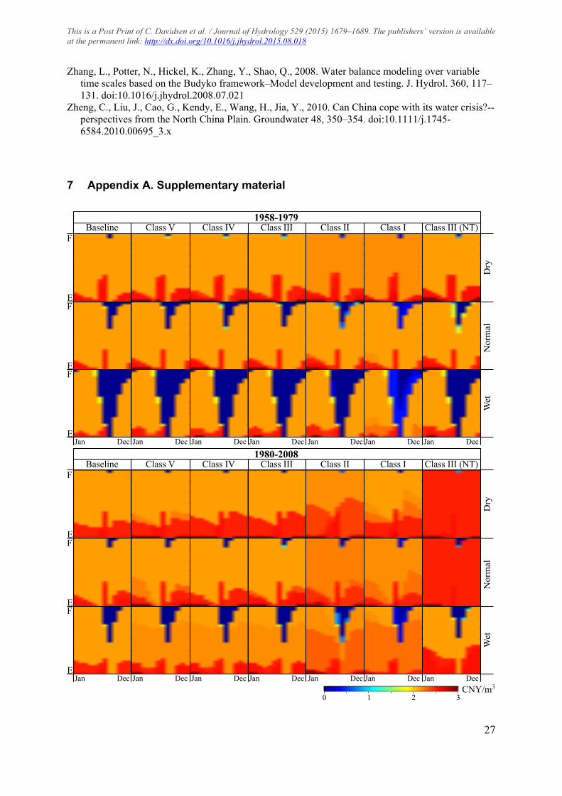
This is a Post Print of C. Davidsen et al. / Journal of Hydrology 529 (2015) 1679–1689. The publishers’ version is available at the permanent link: http://dx.doi.org/10.1016/j.jhydrol.2015.08.018
27
Zhang, L., Potter, N., Hickel, K., Zhang, Y., Shao, Q., 2008. Water balance modeling over variable time scales based on the Budyko framework–Model development and testing. J. Hydrol. 360, 117–131. doi:10.1016/j.jhydrol.2008.07.021
Zheng, C., Liu, J., Cao, G., Kendy, E., Wang, H., Jia, Y., 2010. Can China cope with its water crisis?--perspectives from the North China Plain. Groundwater 48, 350–354. doi:10.1111/j.1745-6584.2010.00695_3.x
7 Appendix A. Supplementary material
� ��� ��� ��� ��� ��
���
���
���
���
��
���
��
���
���
�
� ��� ��� ��� ��� ��
���
���
���
���
��
���
��
���
���
�
�
E
F
E
F
E
F
Baseline1980-2008
Class V Class IV Class III Class II Class I Class III (NT)
Dry
Nor
mal
CNY/m3
3210
Jan Dec Jan Dec Jan Dec Jan Dec Jan Dec Jan Dec Jan Dec
Wet
E
F
E
F
E
F
Baseline1958-1979
Class V Class IV Class III Class II Class I Class III (NT)
Dry
Nor
mal
Jan Dec Jan Dec Jan Dec Jan Dec Jan Dec Jan Dec Jan Dec
Wet