BIS Working Papers · BIS Working Papers are written by members of the ... Mortgage-backed securities (MBS) ... supply driven by mortgage debt and the risk-bearing …

BIS Working PapersNo 532

Mortgage risk and the yield curve by Aytek Malkhozov, Philippe Mueller, Andrea Vedolin and Gyuri Venter

Monetary and Economic Department

December 2015

JEL classification: G12, G21, E43

Keywords: Term Structure of Interest Rates, MBS, Supply Factor

BIS Working Papers are written by members of the Monetary and Economic Department of the Bank for International Settlements, and from time to time by other economists, and are published by the Bank. The papers are on subjects of topical interest and are technical in character. The views expressed in them are those of their authors and not necessarily the views of the BIS.

This publication is available on the BIS website (www.bis.org).

© Bank for International Settlements 2015. All rights reserved. Brief excerpts may be reproduced or translated provided the source is stated.

ISSN 1020-0959 (print) ISSN 1682-7678 (online)

Mortgage Risk and the Yield Curve∗

Aytek Malkhozov† Philippe Mueller‡ Andrea Vedolin§

Gyuri Venter¶

Abstract

We study the feedback from the risk of outstanding mortgage-backed secu-rities (MBS) on the level and volatility of interest rates. We incorporate thesupply shocks resulting from changes in MBS duration into a parsimoniousequilibrium dynamic term structure model and derive three predictions thatare strongly supported in the data: (i) MBS duration positively predictsnominal and real excess bond returns, especially for longer maturities; (ii)the predictive power of MBS duration is transitory in nature; and (iii) MBSconvexity increases interest rate volatility, and this effect has a hump-shapedterm structure.

∗We would like to thank Tobias Adrian, Caio Almeida, Michael Bauer, Ruslan Bikbov, Mike Cher-nov, John Cochrane, Pierre Collin-Dufresne, Jefferson Duarte, Greg Duffee, Mathieu Fournier, AndrasFulop, Robin Greenwood, Sam Hanson, Christian Julliard, Anh Le, Neil Pearson, Douglas McManus,Marcel Rindisbacher, Richard Stanton, Dimitri Vayanos, Nancy Wallace, Paul Whelan, two anonymousreferees, and seminar and conference participants at the Bank of England, Banque de France, CBS,Deutsche Bank, Duke University, Erasmus University, Exeter University, Imperial Business School, LSE,Manchester Business School, the Oxford-MAN Institute, Toulouse School of Economics, LuxembourgSchool of Finance, University of Nottingham, SAC Capital Advisors, University of Bern, Universityof Bonn, 2012 Arne Ryde Workshop, 2012 IFSID Conference on Structured Products and Derivatives,2012 Young Scholars Nordic Finance Workshop, 2012 Junior Faculty Research Roundtable at UNC, 2012Conference on Advances in the Analysis of Hedge Fund Strategies, 2013 Mathematical Finance Days,2013 Bank of Canada Fixed Income conference, 2013 Financial Econometrics conference in Toulouse,2013 SFS Cavalcade, 2013 WFA meetings, 2013 UNC/Atlanta Fed Conference on Housing, 2014 NBERSI AP, and 2015 AFA Meetings for thoughtful comments. Malkhozov gratefully acknowledges finan-cial support from the Institut de Finance Mathematique de Montreal. Mueller and Vedolin gratefullyacknowledge financial support from the LSE Research Committee Seed Fund. Venter gratefully ac-knowledges financial support from the Center for Financial Frictions (FRIC), grant no. DNRF102. Allauthors thank the Paul Woolley Centre at the LSE and the Dauphine-Amundi Chair in Asset Man-agement for financial support. The views expressed in this paper are those of the authors and do notnecessarily reflect those of the Bank for International Settlements.

†Bank for International Settlements, Centralbahnplatz 2, 4002 Basel, Switzerland, Phone: +41 61280 864, Email: [email protected]

‡London School of Economics, Department of Finance, Houghton Street, WC2A 2AE London, UK,Phone: +44 20 7955 7012, Email: [email protected]

§London School of Economics, Department of Finance, Houghton Street, WC2A 2AE London, UK,Phone: +44 20 7955 5017, Email: [email protected]

¶Copenhagen Business School, Department of Finance, Solbjerg Plads 3, 2000 Frederiksberg, Den-mark; Phone: +45 3815 2795, Email: [email protected]

mailto:[email protected]




Mortgage-backed securities (MBS) and, more generally, mortgage loans constitute a

major segment of US fixed income markets, comparable in size to that of Treasuries. As

such, they account for a considerable share of financial intermediaries’ and institutional

investors’ exposure to interest rate risk.1 The contribution of MBS to the fluctuations in

the aggregate risk of fixed income portfolios over short to medium horizons is even more

important. Indeed, because most fixed-rate mortgages can be prepaid and refinanced as

interest rates move, the variation of MBS duration can be very large, even over short

periods of time.2

In this paper we study the feedback from fluctuations in the aggregate risk of MBS

onto the yield curve. To this end, we build a parsimonious dynamic equilibrium term

structure model in which bond risk premia result from the interaction of the bond

supply driven by mortgage debt and the risk-bearing capacity of specialized fixed income

investors.

The equilibrium takes the form of a standard Vasicek (1977) short rate model aug-

mented by an affine factor, aggregate MBS dollar duration, which captures the additional

interest rate risk that investors have to absorb. Intuitively, a fall in mortgage duration

is similar to a negative shock to the supply of long-term bonds that has an effect on

their prices. In addition to duration itself, its sensitivity to changes in interest rates,

measured by aggregate MBS dollar convexity, also plays a role. Because MBS duration

falls when interest rates drop, mortgage investors who aim to keep the duration of their

portfolios constant for hedging or portfolio rebalancing reasons will induce additional

buying pressure on Treasuries and thereby amplify the effect of an interest rate shock.

As a result, the MBS channel can simultaneously affect bond prices and yield volatility.

1Between 1990 and 2014 the average value of outstanding mortgage-related and Treasury debt wasUSD 5tr each. Financial intermediaries and institutional investors hold approximately 25% of the totalamount outstanding in Treasuries, and approximately 30% of the total amount outstanding in MBS.Government-sponsored enterprises (GSEs) hold on average around 13% of all outstanding MBS (seeSecurities Industry and Financial Markets Association (2013) and the Flow of Funds Tables of theFederal Reserve).

2Aggregate MBS duration can drop by more than two years within a six-month period (see alsoFigure 1). The duration of Treasuries does not experience changes of such magnitude over short horizons.Taking into account the value of outstanding mortgage debt, we calculate that a one standard deviationshock to MBS duration is a dollar duration equivalent of a USD 368bn shock to the supply of 10-yearTreasuries.

1

Our model makes a range of predictions for which we find strong empirical evidence.

First, MBS duration predicts both nominal and real bond excess returns. This effect

is stronger for longer maturity bonds that are more exposed to interest rate risk. At

the same time, the effect is weaker for real bonds if real rates are imperfectly correlated

with nominal rates and are less volatile. Accordingly, we find an economically significant

relationship between duration and bond risk premia, in particular at longer maturities:

A one standard deviation change in MBS duration implies a 381 basis point change in

the expected one-year excess return on a 10-year nominal bond and a 199 basis point

change in the expected one-year excess return on a 10-year real bond. These effects

imply an approximately 38 ≈ 381/10 (20) basis point increase in nominal (real) 10-year

yields, assuming that most of the effect on returns happens within a year.

Second, while large in size, shocks to MBS duration and their effect on bond excess

returns are transient. Our model captures the fast mean-reversion in aggregate MBS

duration by linking it to both interest rate mean-reversion and the renewal of the mort-

gage pool through refinancing. For example, running predictive regressions for different

return horizons, we find little additional effect of MBS duration on bond excess returns

beyond one year.

Finally, in our model the feedback between changes in long-term yields and MBS

duration translates into higher yield volatility: Lower interest rates decrease duration,

which in turn decreases the term premium and further lowers long-term rates. Different

from noncallable bonds, callable bonds such as MBS typically feature a concave relation-

ship between prices and yields, the so-called negative convexity. More negative convexity

implies that the duration and, therefore, the market price of risk are more sensitive to

changes in interest rates. Empirically, we find that the effect is hump-shaped and most

pronounced for maturities between two and three years. In terms of magnitude, any one

standard deviation change in MBS dollar convexity changes 2-year bond yield volatility

by approximately 37 basis points. A calibrated version of our model reproduces the

above predictions with similar economic magnitudes.

The statistical significance and the magnitude of our estimates remains stable when

we control for a range of standard predictors of bond risk premia and yield volatility,

2

including yield factors, macroeconomic variables, and bond market liquidity measures.

Overall, we find little overlap between the predictive power of MBS duration and con-

vexity and that of other factors, which justifies the narrow focus of the paper on the

MBS channel.

Our paper builds on the premise that fluctuations in MBS duration prompt fixed

income investors to adjust their hedging positions, rebalance their portfolios, or more

generally revise the required risk premia at which they are willing to hold bonds. To

support this view, we show that the increase in the share of outstanding MBS held

by Fannie Mae and Freddie Mac (government-sponsored enterprises or GSEs) can be

associated with a strengthening of the MBS duration channel, whereas the subsequent

decrease in that share and the increasingly important role of the Federal Reserve made

it weaker. GSEs actively manage their interest rate risk exposure, while the Federal

Reserve has no such objective. These findings are in line with our interpretation of the

main results of the paper.

The MBS channel analyzed in our paper has attracted the attention of practitioners,

policy makers, and empirical researchers alike. Perli and Sack (2003), Chang, McManus,

and Ramagopal (2005), and Duarte (2008) test the presence of a linkage between various

proxies for MBS hedging activity and interest rate volatility. Unlike those papers, we look

at the effect that MBS convexity has on the entire term structure of yield volatilities, and

find that it is strongest for intermediate (and not long, as previously assumed) maturities.

Our model provides an explanation for this finding. In contemporaneous work, Hanson

(2014) reports results similar to ours regarding the predictability of nominal bond returns

by MBS duration. In contrast to the theoretical framework that guides the author’s

analysis, our dynamic term structure model allows us to jointly explain the effect of

mortgage risk on real and nominal bond risk premia, and bond yield volatilities across

different maturities.

Our work is also related to the literature on government bond supply and bond

risk premia. We make use of the framework developed by Vayanos and Vila (2009).

In their model, the term structure of interest rates is determined by the interaction of

preferred habitat investors and risk-averse arbitrageurs, who demand higher risk premia

3

as their exposure to long-term bonds increases. Thus, the net supply of bonds matters.

Greenwood and Vayanos (2014) use this theoretical framework to study the implications

of a change in the maturity structure of government debt supply, similar to the one

undertaken in 2011 by the Federal Reserve during “Operation Twist”. Our paper is

different in at least three respects. First, in our model the variation in the net supply of

bonds is driven endogenously by changing MBS duration, and not exogenously by the

government. Second, the supply factor in Greenwood and Vayanos (2014) explains low

frequency variation in risk premia, because movements in maturity-weighted government

debt to GDP occur at a lower frequency than movements in the short rate. Our duration

factor, on the other hand, explains variations in risk premia at a higher frequency than

movements in the level of interest rates. Finally, Greenwood and Vayanos (2014) posit

that the government adjusts the maturity structure of its debt in a way that stabilizes

bond markets. For instance, when interest rates are high, the government will finance

itself with shorter maturity debt and thereby reduce the quantity of interest rate risk

held by agents. Our mechanism goes exactly in the opposite direction: Because of the

negative convexity in MBS, the supply effect amplifies interest rate shocks.3,4

Our paper is related to Gabaix, Krishnamurthy, and Vigneron (2007), who study the

effect of limits to arbitrage in the MBS market. The authors show that, while mortgage

prepayment risk resembles a wash on an aggregate level, it nevertheless carries a positive

risk premium because it is the risk exposure of financial intermediaries that matters. Our

paper is based on a similar premise. Different from these authors, however, we do not

study prepayment risk, but changes in interest rate risk of MBS that are driven by the

prepayment probability, and their effect on the term structure of interest rates.

The remainder of the paper is organized as follows. Section 1 sets up a model of

the term structure of interest rates and MBS duration, and solves for its equilibrium.

3Corporate debt constitutes another important class of fixed income instruments and its supply hasbeen shown to be negatively correlated with the supply of Government debt. For example, Greenwood,Hanson, and Stein (2010) show that firms choose their debt maturity in a way that tends to offset thevariations in the supply and maturity of Government debt. However, the authors find no relationshipbetween corporate debt and MBS supply, which provides us with an additional motivation to focus onthe latter.

4Domanski, Shin, and Sushko (2015) argue that a negative convexity gap between German insurancesector assets and liabilities gives rise to a similar amplification effect.

4

Section 2 discusses the qualitative predictions of the model. Section 3 describes the data

used and Section 4 empirically tests our hypotheses. Section 5 calibrates the model to

the data and quantitatively confirms our empirical findings. Finally, Section 6 concludes.

Proofs and additional robustness checks are deferred to the Online Appendix.

1 Model

In this section we propose a parsimonious dynamic equilibrium term structure model

in which changes in MBS duration are equivalent to long-term bond supply shocks:

When the probability of future mortgage refinancing increases but before refinancing

happens and investors have access to new mortgage pools, the interest rate risk profile

of mortgage-related securities available to investors resembles that of relatively short

maturity bonds.5

1.1 Bond market

Time is continuous and goes from zero to infinity. We denote the time t price of a zero-

coupon bond paying one dollar at maturity t+ τ by Λτt , and its yield by yτt = − 1

τlog Λτ

t .

The short rate rt is the limit of yτt when τ → 0. We take rt as exogenous and assume

that its dynamics under the physical probability measure are given by

drt = κ (θ − rt) dt+ σdBt, (1)

where θ is the long run mean of rt, κ is the speed of mean reversion, and σ is the volatility

of the short rate.

At each date t, there exists a continuum of zero-coupon bonds with time to maturity

τ ∈ (0, T ] in total net supply of sτt , to be specified below. Bonds are held by financial

institutions who are competitive and have mean-variance preferences over the instanta-

5Market participants can invest in new mortgage loans by buying corresponding MBS. Up to 90days before those MBS are issued, investors have access to them through the “to-be-announced” (TBA)market (see e.g., Vickery and Wright (2010)).

5

neous change in the value of their bond portfolio. If xτt denotes the quantity they hold

in maturity-τ bonds at time t, the investors’ budget constraint becomes

dWt =

(

Wt −∫ T

0

xτtΛ

τt dτ

)

rtdt+

∫ T

0

xτtΛ

τt

dΛτt

Λτt

dτ , (2)

and their optimization problem is given by

max{xτ

t }τ∈(0,T ]

Et [dWt]−α

2Vart [dWt] , (3)

where α is their absolute risk aversion. Since financial institutions have to take the other

side of the trade in the bond market, the market clearing condition is given by

xτt = sτt , ∀t and τ. (4)

The ability of financial institutions to trade across different bond maturities simplifies

the characterization of the equilibrium market price of interest rate risk. From the

financial institutions’ first order condition and the absence of arbitrage, we obtain the

following result:

Lemma 1. Given (1)-(4), the unique market price of interest rate risk is proportional

to the dollar duration of the total supply of bonds:

λt = ασd(

∫ T

0sτtΛ

τt dτ

)

drt. (5)

Lemma 1 implies that in order to derive the equilibrium term structure it is not

necessary to explicitly model the maturity structure of the bond supply, but it is sufficient

to capture its duration.

1.2 MBS duration

The supply of bonds is determined by households’ mortgage liabilities. Without explic-

itly modeling them, we think about a continuum of households who do not themselves

6

invest in bonds but take fixed-rate mortgage loans that are then sold on the market as

MBS. The aggregate duration of outstanding MBS is driven by two forces: (i) changes

in the level of interest rates that affect the prepayment probability of each outstanding

mortgage, and (ii) actual prepayment that changes the composition of the aggregate

mortgage pool. The earlier literature has adopted two main ways of describing pre-

payment behavior: Prepayment can be modelled as an optimal decision by borrowers

who minimize the value of their loans; see, e.g., Longstaff (2005). Alternatively, since

micro-level evidence suggests that individual household prepayment is often non-optimal

relative to a contingent-claim approach, Stanton and Wallace (1998) add an exogenous

delay to refinancing (see also Schwartz and Torous (1989) and Stanton (1995)). In

the following, we posit a reduced-form model of aggregate prepayment in the spirit of

Gabaix, Krishnamurthy, and Vigneron (2007). Our motivation for using a reduced-form

approach is twofold. First, we avoid making strong assumptions regarding the optimal

prepayment. Second, the incentive to prepay on aggregate is well explained by interest

rates themselves.

Households refinance their mortgages when the incentive to do so is sufficiently high.

Prepaying a mortgage is equivalent to exercising an American option. As shown in

Richard and Roll (1989), the difference between the fixed rate paid on a mortgage and

the current mortgage rate is a good measure of the moneyness of this prepayment option.

Because households can have mortgages with different characteristics, we focus on the

average mortgage coupon (interest payment) on outstanding mortgages, ct. Following

Schwartz and Torous (1989), we approximate the current mortgage rate by the long-term

interest rate yτt with reference maturity τ . According to Hancock and Passmore (2010),

it is common industry practice to use either the 5- or 10-year swap rate as a proxy for

MBS duration. To match the average MBS duration, which is 4.5 years in our data

sample, we set τ = 5. In sum, we define the refinancing incentive as ct − yτt .

On aggregate, refinancing activity does not change the size of the mortgage pool:

when a mortgage is prepaid, another mortgage is issued. However, the average coupon

ct is affected by prepayment, because the coupon of the newly issued mortgages depends

7

on the current level of mortgage rates. We assume that the evolution of the average

coupon is a function of the refinancing incentive:

dct = −κc (ct − yτt ) dt, (6)

with κc > 0. This means that a lower interest rate yτt , i.e., a higher refinancing incentive,

leads to more prepayments, and new mortgages issued at this low rate decrease the

average coupon more. Because our focus is the feedback between the MBS market and

interest rates, we also assume that on aggregate there is no additional uncertainty about

refinancing. The upper left panel of Figure 1 provides empirical motivation for (6). We

plot the difference between the 5-year yield and the average MBS coupon, together with

the subsequent change in the average coupon. The two series are closely aligned with

the coupon reacting with a slight delay to a change in the refinancing incentive.

The distinctive feature of mortgage-related securities is that their duration depends

primarily on the likelihood that they will be refinanced in the future. The MBS coupon

and the level of interest rates proxy for the expected level of prepayments and the

moneyness of the option (see Boudoukh, Whitelaw, Richardson, and Stanton (1997)).

We thus assume that the aggregate dollar duration of outstanding mortgages is a function

of the refinancing incentive:

Dt = θD − ηy (ct − yτt ) , (7)

where duration, Dt ≡ −dMBSt/dyτt , is the observable sensitivity of the aggregate mort-

gage portfolio value (MBSt) to the changes in the reference long-maturity rate yτt , and

θD, ηy > 0 are constants. The upper right panel of Figure 1 provides empirical moti-

vation for (7). We plot the difference between the 5-year yield and the average MBS

coupon, together with aggregate MBS duration. The two series are again very closely

aligned. In addition, we consider in Figure 1 (lower left panel) a simple scatter diagram

of the two series. In general, the relationship between interest rates and prepayment is

found to be “S-shaped” (see, e.g., Boyarchenko, Fuster, and Lucca (2014)). We note

that the link between MBS duration and the refinancing incentive is approximately lin-

8

ear, although the relationship becomes more dispersed when interest rates rise and the

option becomes more out-of-the-money. Overall, we conclude that our model captures

well the key stylized properties of aggregate refinancing activity.

[Insert Figure 1 here.]

Combining (6) and (7) gives us the dynamics of Dt:

dDt = κD (θD −Dt) dt+ ηydyτt , (8)

where κD = κc. Note that dollar duration is driven both by changes in long-term interest

rates and refinancing activity. The parameter ηy = dDt/dyτt is the negative of the dollar

convexity: When ηy > 0, lower interest rates increase the probability of borrowers

prepaying their mortgages in the future, leading to a lower duration. The lower right

panel of Figure 1 plots the MBS convexity series showing that in our sample it always

stays negative. Comparative statics with respect to ηy allow us to derive predictions

regarding the effect of negative convexity on interest rate volatility.6

1.3 Discussion

We now discuss bond supply and the identity and behavior of investors within the context

of our model. We understand the former as the net supply of bonds coming from the

rebalancing of fixed income portfolios in response to fluctuations in MBS duration. For

instance, the hedging positions of the GSEs analyzed in Section 4.4 would be one of its

components.

On the other hand, rather than modeling all bond market investors, we abstract from

buy-and-hold investors and focus directly on those who end up absorbing this additional

net supply. In particular, we have in mind financial institutions such as investment

6A model where ηy itself follows a stochastic process would not fall into one of the standard tractableclasses of models. The Online Appendix presents a version of the model that accommodates time-varyingconvexity. While this model implies a quadratic instead of an affine term structure, it leads to identicalqualitative predictions.

9

banks, hedge funds, and fund managers, who specialize in fixed income investments,

trade actively in the bond market, and act as marginal investors there in the short to

medium run.7

The risk-bearing capacity of financial institutions is key to why shocks to MBS

duration matter. The mortgage choice of households determines the supply of fixed

income securities, sτt , through the duration of mortgages, Dt, but in addition to this

channel, households are not present on either side of the market-clearing condition (4).

In other words, except for having a constant amount of mortgage debt, in the model

households do not take part in fixed income markets.8 As a result, the variation in the

supply of bonds induced by changes in MBS duration is not washed out and matters for

bond prices.9

To summarize the mechanism, while lower interest rates trigger a certain amount of

refinancing of the most in-the-money mortgages, they also increase the probability of

future prepayment and, thus, decrease the duration of all outstanding mortgages. In

fact, empirical evidence shows that households’ refinancing is gradual (see Campbell

(2006)). The progressive nature of refinancing (κc < ∞) leaves financial institutions

who invest in MBS on aggregate short of duration exposure after a negative shock to

7The role of financial institutions in our model is similar to Greenwood and Vayanos (2014). Flemingand Rosenberg (2008) find that Treasury dealers are compensated by high excess returns when holdinglarge inventories of newly issued Treasury securities. More generally, financial intermediaries and in-stitutional investors hold approximately 25% of the total amount outstanding in Treasuries, and dailytrading volume is almost 10% of the total amount outstanding. In addition, these financial intermedi-aries hold around 30% of the total amount outstanding in MBS, and daily trading is almost 25% of thetotal amount outstanding. GSEs hold on average around 13% of all outstanding MBS. Data is for theperiod 1997 to 2014; see Securities Industry and Financial Markets Association (2013) and the Flow ofFunds Tables of the Federal Reserve.

8Home mortgages represent approximately 70% of household liabilities. While households invest inTreasuries (their holdings account for approximately 6% of the total amount outstanding in 2014), to thebest of our knowledge, there is no evidence suggesting that they actively manage the duration of theirmortgage liabilities by trading fixed income instruments. Looking at the Flow of Funds Tables of theFederal Reserve we find no relationship between the duration of MBS and the value of households’ bondportfolio either in absolute level or relative to the outstanding amount of Treasuries. Consistent withthis pattern, Rampini and Viswanathan (2015) argue that households’ primary concern is financing,not risk management.

9Gabaix, Krishnamurthy, and Vigneron (2007) make a related point that from the perspective offinancial intermediaries who are the marginal investors in MBS, mortgage prepayment risk cannot behedged and therefore is priced. Note that the prepayment risk of MBS is different from their interestrate risk.

10

interest rates. The opposite happens when interest rates increase and MBS duration

lengthens.

1.4 Equilibrium term structure

Because in the model mortgages underlie the supply of bonds, we replace the dollar

value of bond net supply in (5) with the aggregate mortgage portfolio value MBSt to

obtain

λt = ασdMBSt

drt. (9)

Using a simple chain rule, dMBSt

drt= dMBSt

dyτt

dyτtdrt

, we rewrite (9) in terms of the sensitivity

to the reference long-maturity rate yτt :

λt = −αστyDt, (10)

where στy ≡ dyτt

drtσ, the volatility of yτt , is a constant to be determined in equilibrium.

We look for an equilibrium in which yields are affine in the short rate and the duration

factor. Under the conjectured affine term structure, the physical dynamics of MBS

duration (8) can be written as

dDt = (δ0 − δrrt − δDDt) dt+ ηyστydBt, (11)

where δ0, δr and δD are constants to be determined in equilibrium. In turn, equations

(1), (10) and (11) together imply that the dynamics of the short rate and the MBS

duration factor under the risk-neutral measure are

drt =(

κθ − κrt + ασστyDt

)

dt+ σdBQt and (12)

dDt =(

δ0 − δrrt − δQDDt

)

dt+ ηyστydB

Qt , (13)

where δQD ≡ δD − αηy(

στy

)2.

We now have all the ingredients to solve for the equilibrium term structure.

11

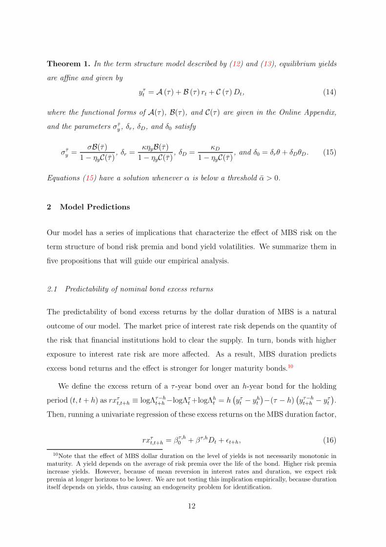
Theorem 1. In the term structure model described by (12) and (13), equilibrium yields

are affine and given by

yτt = A (τ) + B (τ) rt + C (τ)Dt, (14)

where the functional forms of A(τ), B(τ), and C(τ) are given in the Online Appendix,

and the parameters στy , δr, δD, and δ0 satisfy

στy =

σB(τ )1− ηyC(τ )

, δr =κηyB(τ )

1− ηyC(τ ), δD =

κD

1− ηyC(τ ), and δ0 = δrθ + δDθD. (15)

Equations (15) have a solution whenever α is below a threshold α > 0.

2 Model Predictions

Our model has a series of implications that characterize the effect of MBS risk on the

term structure of bond risk premia and bond yield volatilities. We summarize them in

five propositions that will guide our empirical analysis.

2.1 Predictability of nominal bond excess returns

The predictability of bond excess returns by the dollar duration of MBS is a natural

outcome of our model. The market price of interest rate risk depends on the quantity of

the risk that financial institutions hold to clear the supply. In turn, bonds with higher

exposure to interest rate risk are more affected. As a result, MBS duration predicts

excess bond returns and the effect is stronger for longer maturity bonds.10

We define the excess return of a τ -year bond over an h-year bond for the holding

period (t, t+ h) as rxτt,t+h ≡ logΛτ−h

t+h −logΛτt +logΛh

t = h(

yτt − yht)

−(τ − h)(

yτ−ht+h − yτt

)

.

Then, running a univariate regression of these excess returns on the MBS duration factor,

rxτt,t+h = βτ,h

0 + βτ,hDt + ǫt+h, (16)

10Note that the effect of MBS dollar duration on the level of yields is not necessarily monotonic inmaturity. A yield depends on the average of risk premia over the life of the bond. Higher risk premiaincrease yields. However, because of mean reversion in interest rates and duration, we expect riskpremia at longer horizons to be lower. We are not testing this implication empirically, because durationitself depends on yields, thus causing an endogeneity problem for identification.

12

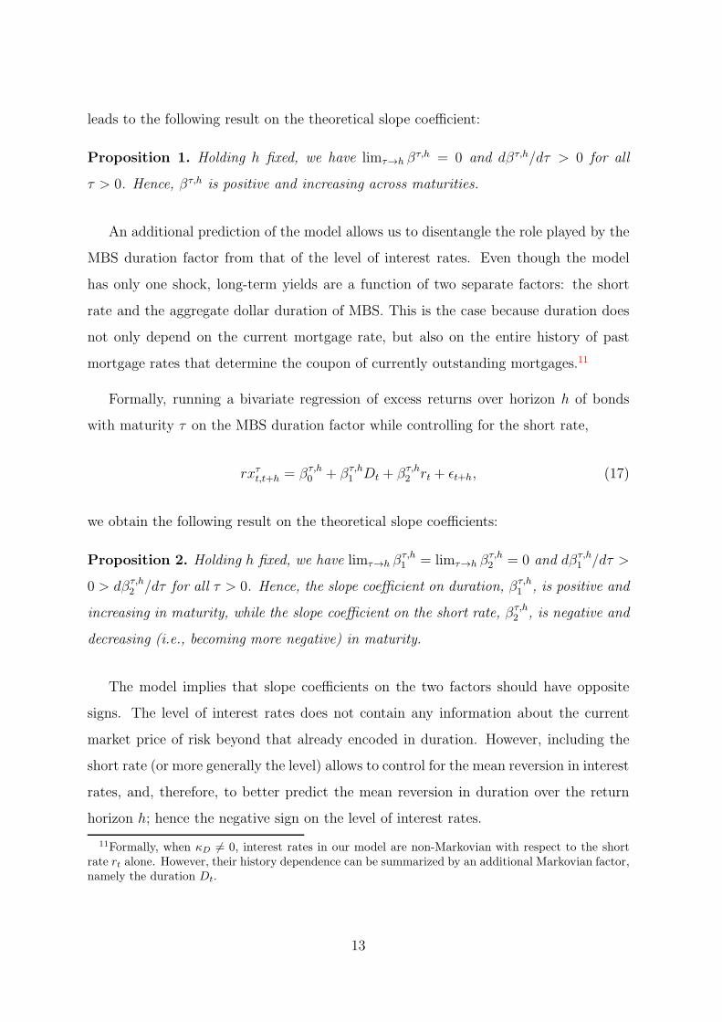
leads to the following result on the theoretical slope coefficient:

Proposition 1. Holding h fixed, we have limτ→h βτ,h = 0 and dβτ,h/dτ > 0 for all

τ > 0. Hence, βτ,h is positive and increasing across maturities.

An additional prediction of the model allows us to disentangle the role played by the

MBS duration factor from that of the level of interest rates. Even though the model

has only one shock, long-term yields are a function of two separate factors: the short

rate and the aggregate dollar duration of MBS. This is the case because duration does

not only depend on the current mortgage rate, but also on the entire history of past

mortgage rates that determine the coupon of currently outstanding mortgages.11

Formally, running a bivariate regression of excess returns over horizon h of bonds

with maturity τ on the MBS duration factor while controlling for the short rate,

rxτt,t+h = βτ,h

0 + βτ,h1 Dt + βτ,h

2 rt + ǫt+h, (17)

we obtain the following result on the theoretical slope coefficients:

Proposition 2. Holding h fixed, we have limτ→h βτ,h1 = limτ→h β

τ,h2 = 0 and dβτ,h

1 /dτ >

0 > dβτ,h2 /dτ for all τ > 0. Hence, the slope coefficient on duration, βτ,h

1 , is positive and

increasing in maturity, while the slope coefficient on the short rate, βτ,h2 , is negative and

decreasing (i.e., becoming more negative) in maturity.

The model implies that slope coefficients on the two factors should have opposite

signs. The level of interest rates does not contain any information about the current

market price of risk beyond that already encoded in duration. However, including the

short rate (or more generally the level) allows to control for the mean reversion in interest

rates, and, therefore, to better predict the mean reversion in duration over the return

horizon h; hence the negative sign on the level of interest rates.

11Formally, when κD 6= 0, interest rates in our model are non-Markovian with respect to the shortrate rt alone. However, their history dependence can be summarized by an additional Markovian factor,namely the duration Dt.

13

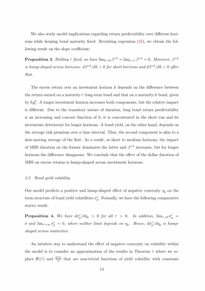
We also study model implications regarding return predictability over different hori-

zons while keeping bond maturity fixed. Revisiting regression (16), we obtain the fol-

lowing result on the slope coefficient:

Proposition 3. Holding τ fixed, we have limh→0 βτ,h = limh→τ β

τ,h = 0. Moreover, βτ,h

is hump-shaped across horizons: dβτ,h/dh > 0 for short horizons and dβτ,h/dh < 0 after

that.

The excess return over an investment horizon h depends on the difference between

the return earned on a maturity-τ long-term bond and that on a maturity-h bond, given

by hyht . A longer investment horizon increases both components, but the relative impact

is different. Due to the transitory nature of duration, long bond return predictability

is an increasing and concave function of h; it is concentrated in the short run and its

increments deteriorate for longer horizons. A bond yield, on the other hand, depends on

the average risk premium over a time interval. Thus, the second component is akin to a

slow-moving average of the first. As a result, at short to medium horizons, the impact

of MBS duration on the former dominates the latter and βτ,h increases, but for longer

horizons the difference disappears. We conclude that the effect of the dollar duration of

MBS on excess returns is hump-shaped across investment horizons.

2.2 Bond yield volatility

Our model predicts a positive and hump-shaped effect of negative convexity ηy on the

term structure of bond yield volatilities στy . Formally, we have the following comparative

statics result:

Proposition 4. We have dστy/dηy > 0 for all τ > 0. In addition, limτ→0 σ

τy =

σ and limτ→∞ στy = 0, where neither limit depends on ηy. Hence, dστ

y/dηy is hump-

shaped across maturities.

An intuitive way to understand the effect of negative convexity on volatility within

the model is to consider an approximation of the results in Theorem 1 where we re-

place B (τ ) and C(τ)α

that are non-trivial functions of yield volatility with constants

14

b = B (τ) |α=0 and c = C(τ)α

|α=0. When cαηy < 1, i.e., the risk aversion is below the

threshold α = 1cηy

, we have an affine equilibrium where the volatility of the reference

maturity yield solves στy = bσ+ cαηyσ

τy . This fixed-point problem is the result of a feed-

back mechanism between long rates and duration: lower interest rates decrease duration,

which in turn decreases the term premium and further lowers long rates. More negative

convexity implies that MBS duration and, therefore, the market price of risk are more

sensitive to changes in interest rates. Through this mechanism the volatility increases

by a factor 11−cαηy

= 1+ cαηy+(cαηy)2+ ... > 1 that captures the combined effect of the

successive iterations of the feedback loop. The feedback explains why negative convexity

can cause potentially significant interest rate volatility even for moderate levels of risk

aversion.

Moreover, the link between convexity and volatility has a term structure dimension.

Short-maturity yields are close to the short rate and therefore are not significantly

affected by variations in the market price of risk. For long maturities, we expect the

duration of MBS to revert to its long-term mean. At the limit, yields at the infinite

horizon should not be affected by current changes in the short rate and MBS duration

at all. As a result, the effect of MBS convexity on yield volatilities has a hump-shaped

term structure.

2.3 Predictability of real bond excess returns

A distinctive feature of MBS duration and, more generally, supply factors is that they

affect the pricing of both nominal and real bonds.12 To the extent that real and nominal

interest rates are correlated, fixed income investors would demand an additional premium

on real bonds when they have to absorb more aggregate duration risk. We extend our

baseline model to study the joint impact of mortgage risk on nominal and real bonds,

with additional details provided in the Online Appendix.

12For instance, Hanson and Stein (2015) argue that the mechanism described in our paper can provideone possible explanation for the sensitivity of long real rates to changes in short nominal rates.

15

We keep our assumptions that the nominal short rate process follows (1) and that

at each date t there exist zero-coupon nominal bonds in time-varying net supply sτt for

all τ ∈ (0, T ]. Further, we assume that a real short rate process under P is given by

dr∗t = κ∗ (θ∗ − r∗t ) dt+ σ∗dB∗t (18)

whose instantaneous correlation with the nominal short rate is dBtdB∗t = ρdt, and that

an inflation index exists and follows

dItIt

= µπt dt− σπdBπ

t , (19)

where dBπt can be correlated with both dBt and dB∗

t . In (19), we set the diffusion of It,

σπ, exogenously, but allow the drift µπt to be any adapted process for now; later we derive

it in equilibrium to satisfy no arbitrage between nominal and real bonds.13 Finally, we

assume that at each date t, there exist a continuum of real zero-coupon bonds with time

to maturity τ ∈ (0, T ] in zero net supply.14

Our assumptions imply that the nominal interest rate sensitivity of all fixed income

securities in the economy is still driven by MBS duration, and so is the risk premium on

nominal bonds; i.e., (5) holds. Furthermore, the equilibrium risk premium on real bonds

depends on how their returns co-move with those on nominal bonds. Hence, equilibrium

nominal yields are given by (14), as before, and we show that real yields are affine in

MBS duration and the nominal and real short rates.

In this generalized setting, running a univariate regression of the horizon-h excess

return of a real bond with maturity τ over that of the maturity-h real bond on the MBS

duration factor,

rxτ∗t,t+h = βτ,h∗

0 + βτ,h∗Dt + ǫt+h, (20)

13In particular, we obtain that the ex-ante Fisher relation holds in equilibrium: the risk-neutral drift,µπQt , must equal the difference between the nominal and real short rates; see the Online Appendix.14For our sample period the size of the TIPS market does not exceed 5% of the outstanding nominal

Treasuries and MBS, suggesting that fixed income investors’ portfolios are primarily exposed to thenominal interest rate risk.

16

and contrasting the loading with the theoretical slope coefficient βτ,h obtained for the

nominal bond, we get the following result:

Proposition 5. When κ∗ ≈ κ, we have βτ,h∗ ≈ ρσ∗

σβτ,h.

Propositions 1 and 5 together imply that the duration coefficients in regression (20)

are positive and increasing with maturity, mirroring the predictions for nominal bonds.

In particular, for any shock in MBS duration, risk premia on real bonds move ρσ∗/σ for

one with risk premia on nominal bonds, where the ratio ρσ∗/σ represents the coefficient

from a regression of real short rate innovations on nominal short rate innovations. Thus,

estimated coefficients for real bonds are smaller than for nominal bonds if real rates are

imperfectly correlated with nominal rates and less volatile.

3 Data

Data is monthly and spans the time period from December 1989 through December

2012.

We use estimates of MBS duration, convexity, index, and average coupon from Bar-

clays available through Datastream.15 The Barclays US MBS index covers mortgage-

backed pass-through securities guaranteed by Ginnie Mae, Fannie Mae, and Freddie

Mac. The index is comprised of pass-throughs backed by conventional fixed rate mort-

gages and is formed by grouping the universe of over one million agency MBS pools

into generic pools based on agency, program (i.e., 30-year, 15-year, etc.), coupon (e.g.,

6.0%, 6.5%, etc.), and vintage year (e.g., 2011, 2012, etc.). A generic pool is included in

the index if it has a weighted-average contractual maturity greater than one year and

more than USD 250m outstanding. We construct measures of dollar duration and dollar

convexity by multiplying the duration and convexity time series with the index level.16

The upper right panel of Figure 1 depicts MBS dollar duration and the lower right

panel plots MBS dollar convexity. Dollar duration and dollar convexity are calculated as

15Datastream tickers for MBS duration and convexity are LHMNBCK(DU) and LHMNBCK(CK),respectively.

16In the following, units are expressed in US dollars assuming that the portfolio value is equal to theindex level in dollars.

17

the product of the Barclays US MBS index level and duration and convexity, respectively.

Overall, the average MBS dollar duration is 457.43 with a standard deviation of 59.85

and the average dollar convexity is -163.73 with a standard deviation of 57.23.17 Table

1 presents a summary statistic of all main variables used.

[Insert Table 1 and Figure 1 here.]

We use the Gurkaynak, Sack, and Wright (2007, GSW henceforth) zero-coupon nomi-

nal yield data available from the Federal Reserve Board. We use the raw data to calculate

annual Treasury bond excess returns for 2- to 10-year bonds. We also download interest

rate swap data from Bloomberg from which we bootstrap a zero-coupon yield curve.

To calculate real bond excess returns, we use liquidity-adjusted real bond yields (see

D’Amico, Kim, and Wei (2014)).18

We denote the annual return between time t and one year later on a τ -year bond

with price Λτt by rτt,t+1y = log Λτ−1y

t+1y − log Λτt . The annual excess bond return is then

defined as rxτt,t+1y = rτt,t+1y − y1yt , where y1yt = − log Λ1y

t is the one-year yield. From

the same data, we also construct a tent-shaped factor from forward rates, the Cochrane

and Piazzesi (2005) factor (CP factor, labeled cpt). Real annual excess bond returns are

denoted by rxτ∗t,t+1y.

Using the GSW yields ranging from one to ten years, we estimate a time-varying

term structure of yield volatility. We sample the data at the monthly frequency and

take monthly log yield changes. We then construct rolling window measures of realized

volatility using a 12-month window which represent the conditional bond yield volatility.

The resulting term structure of unconditional volatility exhibits a hump shape consistent

with the stylized facts reported in Dai and Singleton (2010), with the volatility peak

being at the two-year maturity (see Table 1, Panel C).

Choi, Mueller, and Vedolin (2014) calculate measures of model-free implied bond

market volatilities for a one-month horizon using Treasury futures and options data from

17Units are expressed in dollars assuming that the portfolio value is equal to the index level in dollars.18We find similar results when using liquidity-adjusted real bond yields from Pflueger and Viceira

(2015). We thank Min Wei and Carolin Pflueger for sharing the data with us.

18

the Chicago Mercantile Exchange (CME). We use their data for the 30-year Treasury

bond and henceforth label this measure tivt.

From Bloomberg, we also get implied volatility for at-the-money swaptions for dif-

ferent maturities ranging from one to ten years and we fix the tenor to ten years. We

label these volatilities ivτ10y. Further, we collect implied volatilities on 3-month-maturity

swaptions with tenors ranging between 1 and 10 years, denoted by iv3mτ .

As a proxy of illiquidity in bond markets, we use the noise proxy from Hu, Pan,

and Wang (2013), which measures an average yield pricing error from a fitted yield

curve. As a proxy for economic growth we use the three-month moving average of

the Chicago Fed National Activity Index. Negative (positive) values indicate a below

(above) average growth. We also use a measure of inflation proxied by the consensus

estimate of professional forecasts available from Blue Chip Economic Forecasts.

4 Empirical analysis

In this section we study the predictive power of MBS dollar duration and convexity

for bond excess returns (nominal and real) and bond yield volatility. We start with

univariate regressions to document the role of our main explanatory variables. Then,

for robustness and to address a potential omitted variable bias, we also control for other

well-known predictors of bond risk premia and interest rate volatility. We find that not

only MBS duration and convexity remain statistically significant, but also the economic

size of the coefficients stays stable across different specifications.

The start date for volatility regressions is dictated by the availability of the MBS

convexity time series that starts in January 1997. Daily data for TIPS is available from

the Federal Reserve Board website starting in January 1999, which is the start date for

the real bond return regressions. For all other regressions we start in December 1989.

With each estimated coefficient, we report t-statistics adjusted for Newey and West

(1987) or Hansen and Hodrick (1980) standard errors. The lag length is set to 18.

19

4.1 Nominal bond risk premia

Hypothesis 1. A regression of bond excess returns on the duration of MBS yields a

positive slope coefficient for all maturities. Moreover, the coefficients are increasing in

bond maturity and remain significant when we control for the level of interest rates.

This hypothesis is derived from Propositions 1 and 2. To test it, we run linear

regressions of annual excess returns on the duration factor. The regression is as follows:

rxτt,t+1y = βτ

0 + βτ1durationt + βτ

2 levelt + ǫτt+1y,

where durationt is MBS dollar duration and levelt is the one-year yield. The univariate

results are depicted in the upper two panels of Figure 2, which plot the estimated slope

coefficients of duration, βτ1 (upper left panel), and the associated adjusted R2 (upper

right panel). Both univariate and multivariate results are presented in Table 2.

[Insert Figure 2 and Table 2 here.]

The univariate regression results indicate that MBS duration is a significant pre-

dictor of bond excess returns across all maturities. In line with the theoretical pre-

diction, the coefficient has a positive sign and is increasing with maturity.19 The es-

timated coefficients are also economically significant, especially for longer maturities.

For example, for any one standard deviation increase in MBS dollar duration, there is a

0.0636×59.85 = 381 (slope coefficient times standard deviation of MBS dollar duration)

19We can also test whether the estimated slope coefficients are monotonically increasing using themonotonicity test developed by Patton and Timmermann (2010), i.e., we can test whether

H0 : β10y1

≤ β9y1

≤ · · · ≤ β2y1

versusH1 : β10y

1> β

9y1

> · · · > β2y1,

where βτ1, τ = 2, . . . , 10 years are estimated slope coefficients from an univariate regression from bond

excess returns with maturity τ onto MBS dollar duration. First, note that the spread between thecoefficients on the 2-year and 10-year bond excess returns is 0.0577. The associated t-statistic is 4.26and is therefore statistically highly significant. Turning to the tests for monotonicity, using 10,000bootstrap iterations, we find that the p-value is almost zero and we hence strongly reject the nullhypothesis of no monotonic relationship between estimated coefficients.

20

basis point increase in the expected 10-year bond excess returns. Adjusted R2s range

from 7% for the shortest maturity to 23% for the longest maturity.20 To put these effects

into perspective, we can translate the above numbers into the yield space: for any one

standard deviation change in MBS duration, there is a 381/10 ≈ 38 basis point increase

in the 10-year yield, assuming that most of the effect on returns happens within the first

year (which we verify in the data below).21

One might suspect that the predictive power of MBS duration could result from its

close relationship to the level of interest rates. Proposition 2, however, allows us to

disentangle the contribution of the two factors. To this end, we include the latter as a

control in our multivariate test. The results presented in Table 2 indicate that the slope

coefficient on duration remains positive and increasing with maturity, while the slope

coefficient on the level of interest rates is negative and decreasing for longer maturities.

This is in line with our theory, where the level of interest rates is not directly related to

bond risk premia, but helps to predict the mean reversion in duration at longer horizons,

and, thus, its coefficients have the opposite sign.

Finally, we study the persistence of the MBS dollar duration effect on bond risk

premia by varying the horizon of excess bond returns in our predictive regression:

rx10yt,t+h = β0 + β1durationt + ǫt+h,

where h is 3, 6, 12, 24, and 36 months, respectively. We formulate the following hypoth-

esis in line with Proposition 3:

Hypothesis 2. A regression of bond excess returns on the duration of MBS yields co-

efficients that are hump-shaped across horizons, i.e., they are largest for intermediate

horizons.


20Our conclusions remain the same when we use interest rate swaps instead of Treasury data, andthe duration of the Bank of America US Mortgage Master index (Bloomberg ticker M0A0) instead ofBarclays data (see the Online Appendix).

21One can also relate this to the 91 basis point estimated effect on the 10-year yield of the QE1 program(see Gagnon, Raskin, Remache, and Sack (2010)) whose dollar duration impact is approximately twicethat of a one standard deviation MBS dollar duration shock.

21

The results are presented in Figure 3. We find that coefficients increase up to approx-

imately a one-year horizon, but then plateau and decrease, suggesting that the effect

of MBS duration on bond returns is transitory. Our model provides one possible ex-

planation for this: both the mean reversion in interest rates and refinancing activity

contribute to the fast mean reversion in aggregate MBS duration. The short-lived effect

of MBS duration on bond returns could also be explained by the dynamics of arbitrage

capital that, while slow-moving, ultimately flows into fixed income markets to absorb ad-

ditional duration risk.22 While both factors are likely to play a role, Section 5 presents a

calibration of our model that can quantitatively account for the pattern of multi-horizon

regression coefficients.

4.2 Real bond risk premia

According to our model, the variation in MBS duration should affect the pricing of both

nominal and real bonds. This prediction allows us to differentiate between duration and

factors that are related exclusively to inflation risk. To this end, we test the following

hypothesis based on Propositions 1 and 5:

Hypothesis 3. A regression of real bond excess returns on the duration of MBS yields

a positive slope coefficient that is increasing with maturities. Moreover, real slope coef-

ficients are approximately equal to nominal slope coefficients adjusted by the correlation

between real and nominal rates times the ratio of their volatilities.

Univariate results are presented in Figure 2 (middle two panels) and Table 3. We

find that MBS dollar duration significantly predicts real bond excess returns at longer

maturities. For instance, for the 10-year real bond, the estimated coefficient is positive,

highly significant, and implies that any one standard deviation change in MBS dollar

duration leads to a 0.0293 × 68.25 = 199 (regression coefficient times the standard

deviation of MBS dollar duration between 1999 and 2013) basis point change in real

excess returns.

22See, for example, Greenwood, Hanson, and Liao (2015), who study slow-moving capital in partiallysegmented markets.

22

The relative magnitude of real and nominal coefficients supports a duration risk

explanation of return predictability. Over our sample period from 1999 to 2013, real

rates are less volatile than nominal rates (σ⋆

σ≈ 0.72) and the two series exhibit less

than perfect correlation (ρ ≈ 0.87). Accordingly, the effect of duration on real bond

returns is lower. For the 10-year maturity, the ratio of real to nominal coefficients is

199/341 = 0.58, in line with the 0.87× 0.72 = 0.62 predicted by our theory.23

[Insert Table 3 here.]

4.3 Bond yield volatility

Proposition 4 allows us to formulate the following hypothesis regarding the effect of

MBS convexity on bond yield volatility across maturities:

Hypothesis 4. A regression of conditional yield volatility on the negative convexity of

MBS results in a positive slope coefficient for all maturities. Moreover, the coefficients

are the largest for intermediate maturities, i.e., they have a hump-shaped term structure.

Due to the amplification channel described earlier, we expect a more negative con-

vexity of MBS to result in larger bond yield volatility. To this end, we run the following

univariate regression from conditional bond yield volatility onto MBS convexity:

volτt = βτ0 + βτ

1 convexityt + ǫτt ,

where volτt is the conditional bond yield volatility at time t of a bond with maturity

τ = 1, . . . , 10 years.

The univariate results are presented in the lower two panels of Figure 2 and in

Table 4. In line with our intuition, we find a significant effect from convexity onto bond

23Following the model, these numbers are based on changes in short real and nominal yields. 10-yearyields are more highly correlated, but imply a similar overall ratio of coefficients 0.97 × 0.65 = 0.63.The 341 basis point effect from MBS duration onto the 10-year nominal bond risk premium is for the1999 to 2013 period.

23

yield volatility, and the effect is most pronounced for intermediate maturities.24 The

estimated slope coefficients produce the hump-shaped feature similar to the one observed

in the unconditional averages of yield volatility. Adjusted R2s range from 19% for the

shortest maturities, increase to 22% for the two- and three-year maturities, and decrease

again to 14% for longer maturities. Estimated coefficients are not only statistically but

also economically significant: For the two-year maturity, any one standard deviation

change in MBS dollar convexity is associated with a 37 (= 0.0764 (slope coefficient) ×57.23 (standard deviation of MBS dollar convexity) × 2.43 (level of 2-year yield) ×

√12)

basis point increase in annual bond yield volatility.


An obvious concern with our regression results is that negative convexity could itself

depend on volatility. Note, that it is a priori unclear in which direction volatility affects

convexity as this depends on whether a particular MBS is in-, out-, or at-the-money.25

For an at-the-money MBS, an increase in volatility will lead to an increase in negative

convexity. Discount (i.e., small negative to positive convexity) and premium (negative

convexity) mortgages will in general have a much lower sensitivity to changes in volatility,

and the effect could go in the opposite direction.26

To address causality, we run Granger tests between MBS dollar convexity and volatil-

ity and present the results in Figure 4. In the left panel, we plot F-statistics of Granger

causality tests that assess the null hypothesis whether negative convexity does not

Granger cause volatility. On the right panel, we plot the corresponding F-statistics

of the reversed Granger regression, i.e., we test the null hypothesis whether volatility

does not Granger cause negative convexity. We also plot the 10% critical values. We

24While there are no formal procedures which specifically test for a hump-shape, we can test whetherthe estimated coefficient on the 2-year bond yield volatility is statistically different from the 3-yearvolatility. Indeed, the difference, which is 0.0192, has a t-statistic of 2.75 and is hence different fromzero. We can then again test for monotonicity between the 3-year and 10-year coefficients. Using theprocedure from Patton and Timmermann (2010), we strongly reject the null of no relationship as thep-value is basically zero.

25This is analogous to the Zomma (sensitivity of an option’s Gamma with respect to changes in theimplied volatility) for equity options.

26We thank Bruce Phelps at Barclays Capital for insightful discussions on this.

24

note that for standard confidence levels, we can reject the null of no Granger causality

from convexity to volatilities for any maturity. On the other hand, longer-maturity yield

volatility does seem to Granger cause convexity as indicated by the F-statistics.


4.4 Two MBS investor types: the GSEs and the Federal Reserve

Our paper builds on the premise that fluctuations in MBS duration prompts investors

to adjust their hedging positions, rebalance their portfolios, or, more generally, revise

the required risk premia at which they are willing to hold bonds. While we do not

observe the behavior of all mortgage investors, we can gauge the validity of the duration

channel by looking at market participants with well-defined institutional mandates, and

test whether the change in the composition of MBS ownership over time has an effect

on expected bond returns.

The two GSEs, Fannie Mae and Freddie Mac, play a central role in the US housing

finance system. In addition to their business of issuing and providing credit guarantee

for a large fraction of pass-through MBS, these institutions also retain a significant

portfolio of mortgage loans and MBS. Unlike that of the guaranteed portfolio, all of the

interest rate risk of the retained portfolio lies with the GSEs. Moreover, Fannie Mae

and Freddie Mac see the hedging of this exposure as part of their mandate, including

the part driven by mortgage prepayment.27 Hedging is done through interest rate swaps

under which they trade the fixed-rate interest payments of mortgage loans for floating-

rate interest rate payments that correspond more closely to their short-term borrowing

costs. To hedge prepayment risk, the GSEs issue callable debt and buy swaptions. If

interest rates fall, the GSEs can redeem their callable debt at lower rates, or similarly,

exercise their swaptions. Historically, the GSEs have started hedging during the 1990s

(see Howard (2013)).

27Fannie Mae specifically stress this fact in the 10K filings. They write “Risk management derivativeinstruments are an integral part of our management of interest rate risk. We supplement our issuance ofdebt securities with derivative instruments to further reduce duration risk, which includes prepaymentrisk. We purchase option-based risk management derivatives to economically hedge prepayment risk.”

25

The top panel of Figure 5 illustrates the relationship between the notional value

of the GSEs’ derivative contracts and MBS duration.28 We note that the value of the

hedging position on average exceeds one trillion USD, and its peaks coincide with the

large drops in MBS duration around 2003 and 2008.

The middle panel of Figure 5 shows the growth of Fannie Mae and Freddie Mac’s

retained portfolio from approximately USD 200bn in the 1990s to almost USD 1.6tr in

2003. The increase in the GSEs’ retained portfolio occurred in parallel with the overall

growth of the MBS and Treasury markets. The bottom panel of Figure 5 presents the

value of the retained portfolio as a share of total outstanding MBS. We note that the

fraction of MBS held by the GSEs is positively associated with the predictive power of

MBS duration on bond excess returns, with both increasing until the mid-2000s and

falling subsequently. While we do not observe the portfolio of other MBS investors

(with an important exception of the Federal Reserve considered below), this evidence

supporting the role of actively hedging GSEs is in line with the MBS duration channel.29


Whereas the GSEs represent a class of investors who actively manage the interest

rate exposure of their MBS portfolio, the Federal Reserve does not aim to hedge the

duration risk of its MBS holdings. On 7 September 2008 the Federal Housing Finance

Agency (FHFA) together with the Treasury outlined a plan to (i) place both GSEs into

conservatorship and (ii) having the Treasury enter into senior preferred stock purchase

agreements with both firms. The latter require both Fannie Mae and Freddie Mac to

wind down their retained investment portfolio at a rate of at least 10% per year until they

each fall below USD 250bn. This large reduction in the actively hedged GSE portfolios

is partly offset by the increase in Federal Reserve holdings (see Malz, Schaumburg,

Shimonov, and Strzodka (2014)). As of end 2014, the Federal Reserve holds USD 1.7tr

of agency MBS.

28According to the Financial Accounting Standard (FAS) 133, any firm is required to publish the fairvalue of derivatives designated as hedging instruments.

29At the same time, the GSEs holdings data is available to us only at an annual frequency, makingmore formal statistical inference difficult.

26

To study the effect of this shift in MBS ownership from the GSEs to the Federal

Reserve on bond risk premia, we run the following regression:

rxτt,t+1y = βτ


2 fed sharet + βτ3durationt × fed sharet + ǫτt,t+1y ,

where fed sharet is the Federal Reserve’s share of total MBS holdings. If the effect of

MBS duration is dampened as the Federal Reserve’s share goes up, we would expect the

loading on the interaction term, βτ3 , to be negative.

The results in Table 5 reveal that the coefficient on MBS duration is still highly

significant and increasing with maturity. In line with our intuition that the increased

MBS holdings of the Federal Reserve have weakened the duration channel, we find

a significant and negative coefficient on the interaction term that is increasing with

maturity.


4.5 MBS duration and other predictors of bond returns

In this section we study MBS duration in relation to other predictors of bond returns

proposed by the literature but not included in our model. First, mortgage refinanc-

ing decisions and hence MBS duration could be a function of the information already

contained in the yield curve. We run the following regression:

rx10yt,t+1y = β0 + β1durationt + β2levelt + β3slopet + β4curvet + ǫt+1y ,

where levelt, slopet and curvet are the first three yield PCs. Table 6 (column 1) reveals

that the economic and statistical significance of the duration factor remains very close

to the results reported in Table 2. In the second column, we control for the Cochrane

and Piazzesi (2005) factor, which is a linear combination of forward rates. Again, we

note that MBS dollar duration is highly significant.


27

MBS duration could also be related to the business cycle as empirical evidence shows

that the refinancing incentive of mortgage holders depends on the economic state (see,

e.g., Chen, Michaux, and Roussanov (2013)). Therefore we control for business cycle

measures that have also been shown to have a significant bearing on bond returns,

namely economic growth and inflation.30 We run the following regression:

rx10yt,t+1y = β0 + β1durationt + β2inflationt + β3growtht + ǫt+1y .

The results are presented in Table 6 (third column). Again, we find that estimated

coefficients remain very similar to the baseline regression results presented in Table 2.

Finally, the last column presents regression results when including both yield and macro

factors; we find MBS duration to remain highly statistically significant.

We conclude that the predictive power of MBS duration is not subsumed by either

yield or macroeconomic factors and constitutes a separate channel. We also note that

shocks to MBS duration are much more transient than shocks to either first two yield

PCs or macro variables. For example, we find that MBS dollar duration has a half-life of

around 4 months, whereas the level, slope, inflation, and growth factors have a half-life

of 83, 23, 15, and 14 months, respectively.

4.6 MBS convexity, other determinants of yield volatility, and swaption implied volatil-

ity

We now control for additional determinants of yield volatility that have been documented

in the literature. For example, it is well-known that volatility tends to increase in

periods of high illiquidity (see, e.g., Hu, Pan, and Wang (2013)). In our multivariate

specification, we therefore add a proxy for illiquidity and a proxy of fixed-income implied

volatility, similar to the VIX in equity markets. We run the following regression from

conditional bond yield volatility onto MBS dollar convexity and a set of other predictors:


1convexityt + βτ2 illiqt + βτ

3 tivt + ǫτt ,

30See e.g., Joslin, Priebsch, and Singleton (2014). We also use the eight principal components frommacro variables as in Ludvigson and Ng (2009) and find that our results remain unchanged.

28

where volτt is the conditional bond yield volatility at time t of a bond with maturity

τ = 1, . . . , 10 years, illiqt is the illiquidity factor at time t, and tivt is the Treasury-

implied volatility at time t. Results are reported in Table 7 (panel A). We find that when

we add illiquidity and tiv to the regression, convexity still remains highly statistically

significant. The estimated coefficients in the bond yield volatility regressions reveal that

the effect is largest for the intermediate maturity of two years as indicated by the size

of the coefficient. All three factors together explain between 27% and 43% of the time

variation in bond yield volatility across different maturities.

[Insert Tables 7 here.]

As hedging can potentially take place both in the bond and in the fixed-income

derivatives market, we also test the impact of MBS dollar convexity on measures of

implied volatility from swaptions. For example, Wooldridge (2001) notes that non-

government securities were routinely hedged in the Treasury market until the financial

crisis of 1998 when investors started hedging their interest rate exposure in the swaptions

market.

Table 7, panels B and C present estimated coefficients when regressing either implied

volatility of τ -maturity swaptions written on the 10-year swap rate (panel B) or implied

volatility of 3-month swaptions written on τ -maturity swap rates (panel C). We find that

the effect is stronger for shorter maturities and tenors, and all coefficients are positive

and highly significant.

5 Calibration

In this section we calibrate our model to test its quantitative performance.

5.1 Estimated and calibrated parameters

We estimate the parameters of the short rate process (1), real short rate (18), and the

dollar duration process (8). We note that equation (8) provides a very good description

29

of the monthly series of MBS dollar duration as the associated R2 is 83%. In order to

fully characterize the theoretical effect of MBS duration and convexity on bond returns

and yield volatility, we set the risk aversion of financial institutions to α = 88. This

value allows the model to match the R2 of the predictive regression of 10-year nominal

bond excess returns on duration reported in Table 2. Note that α is the coefficient

of absolute risk aversion. In order to interpret this value, we multiply it by financial

institutions’ wealth to obtain a coefficient of relative risk aversion. In a setting similar to

ours, Greenwood and Vayanos (2014) use financial institutions’ capital to GDP ratio of

13.3%. Because we use the dollar duration of the MBS index to calibrate the model and

the average value of the index itself is standardized to one dollar, we also need to adjust

for the size of the MBS market relative to GDP. Between 1997 and 2012 the average

value of outstanding mortgage-related debt was equal to 53% of the GDP. This implies

a coefficient of relative risk aversion of approximately 22 ≈ 88× 13.3%/53%.

We summarize all calibrated parameter values in Table 8.


5.2 Return predictability and volatility

The calibrated model provides a benchmark for the empirical results in Section 4. The

two top panels of Figure 6 report the term structure of theoretical βτ,h and βτ,h∗ together

with our empirical estimates. The coefficients implied by the model are within the 95%

confidence intervals for maturities up to 8 years, but it underpredicts them at the long

end.

The lower left panel of Figure 6 reports the theoretical slope coefficients β10y,h for

different return horizons. In line with our empirical estimates, the coefficients increase

steeply up to approximately one year before they plateau and then decrease. This

suggests that the mean reversion in aggregate MBS dollar duration is enough to account

for the transitory nature of its effect on bond returns.

The lower right panel of Figure 6 reports the total change in yield volatility across

maturities that can be attributed to negative convexity. For instance, the calibrated

30

model implies a 48 basis point increase in the two-year yield volatility relative to the

case where the negative convexity channel is shut down. This can be compared to the

estimated 131 basis point change in the two-year yield volatility that would result from

a 2.9-standard-deviation shock bringing convexity from its average value to zero.31 In

line with our empirical findings, the calibrated model implies that the effect of negative

convexity is hump-shaped and strongest for maturities around two and three years.


5.3 MBS duration and the cross-section of yields

We also look at the ability of the calibrated model to match additional stylized facts

regarding the information in MBS duration and its relation to the information encoded

in yields. Table 6 reveals that the predictive power of our duration factor remains largely

unaffected when we control for the first three principal components of yields. Moreover,

regressing duration on these yield factors results in an R2 of a mere 22%.

While our stylized model is not designed to address the possibility that MBS duration

is unspanned, the calibration exercise nevertheless speaks to the empirical facts. In the

calibrated model the short rate factor explains over 96% of the variation in yields across

maturities, but only around 7% of the variation in MBS duration and only around 1% of

the one-year excess return on the 10-year bond. At the same time, duration accounts for

all the return predictability and explains the same proportion of 10-year bond returns

(R2 = 24%) in the model as in the data. In other words, the factor that accounts for all

the predictive power is not strongly related to the factor that accounts for a dominant

fraction of the cross sectional variation in yields.

31One reason the model underpredicts the basis point effect of convexity is that it produces a lowerlevel of interest rate volatility compared to the data, and hence the volatility amplification mechanismis applied to a lower base level of volatility.

31

6 Conclusion

In this paper we study both theoretically and empirically the feedback from the fluc-

tuations of aggregate MBS risk onto the yield curve. Our model makes the following

predictions. First, MBS duration increases both nominal and real bond excess returns

and the effect is strongest for longer maturities. Second, the predictive power of MBS

duration for bond excess returns is transient. Third, MBS convexity positively affects

bond yield volatilities and the relationship is hump-shaped across maturities.

We test these predictions in the data and find strong support. In particular, any

one standard deviation change in MBS duration increases expected annual 10-year bond

returns by 381 basis points, while real bond returns increase by 199 basis points. Since

the effect of MBS duration on expected returns is transient in nature and becomes

insignificant for a horizon beyond one year, this translates to a rise in nominal (real) 10-

year yields of 38 (20) basis points today. Our results are comparable in magnitude to the

impact of the recent Quantitative Easing programs implemented by the Federal Reserve:

the cumulative effect of all large-scale asset purchases taken together is estimated to

be between 80 and 120 basis points (see Stein (2012)). For volatility, we find that a

one standard deviation change in MBS convexity, changes 2-year bond yield volatility

by 37 basis points. Finally, we calibrate our model to the data and find that our

model successfully produces effects which are quantitatively in line with their empirical

counterparts.

32

References

Boudoukh, J., R. F. Whitelaw, M. Richardson, and R. Stanton (1997): “PricingMortgage-Backed Securities in a Multifactor Interest Rate Environment: A MultivariateDensity Estimation Approach,” Review of Financial Studies, 10, 405–446.

Boyarchenko, N., A. Fuster, and D. O. Lucca (2014): “Understanding MortgageSpreads,” Working Paper, Federal Reserve Bank of New York.

Campbell, J. Y. (2006): “Household Finance,” Journal of Finance, 61, 1553–1604.

Chang, Y., D. McManus, and B. Ramagopal (2005): “Does Mortgage Hedging RaiseLong-Term Interest Rate Volatility?,” Journal of Fixed Income, 14, 57–66.

Chen, H., M. Michaux, and N. Roussanov (2013): “Houses as ATMs? Mortgage Refi-nancing and Macroeconomic Uncertainty,” Working Paper, MIT.

Choi, H., P. Mueller, and A. Vedolin (2014): “Bond Variance Risk Premiums,” WorkingPaper, London School of Economics.

Cochrane, J. H., and M. Piazzesi (2005): “Bond Risk Premia,” American Economic

Review, 95, 138–160.

Dai, Q., and K. Singleton (2003): “Term Structure Dynamics in Theory and Reality,”Review of Financial Studies, 16, 631–678.

D’Amico, S., D. H. Kim, and M. Wei (2014): “Tips from TIPS: the informational contentof Treasury Inflation-Protected Security prices,” Working Paper, Federal Reserve Board.

Domanski, D., H. Shin, and V. Sushko (2015): “The hunt for duration: not waving butdrowning?,” Bank of International Settlement, Working Paper No 519.

Duarte, J. (2008): “The Causal Effect of Mortgage Refinancing on Interest Rate Volatility:Empirical Evidence and Theoretical Implications,” Review of Financial Studies, 21, 1698–1731.

Fleming, M. J., and J. V. Rosenberg (2008): “How Do Treasury Dealers Manage TheirPositions?,” Working Paper, Federal Reserve Bank of New York.

Gabaix, X., A. Krishnamurthy, and O. Vigneron (2007): “Limits of Arbitrage: Theoryand Evidence from Mortgage-Backed Securities Market,” Journal of Finance, 62, 557–595.

Gagnon, J. E., M. Raskin, J. Remache, and B. P. Sack (2010): “Large-Scale AssetPurchases by the Federal Reserve: Did They Work?,” Working Paper, Board of Governorsof the Federal Reserve System.

Greenwood, R., S. G. Hanson, and G. Y. Liao (2015): “Price Dynamics in PartiallySegmented Mark,” Working Paper, Harvard Business School.

Greenwood, R., S. G. Hanson, and J. C. Stein (2010): “A Gap-Filling Theory ofCorporate Debt Maturity Choice,” Journal of Finance, 65, 993–1028.

Greenwood, R., and D. Vayanos (2014): “Bond Supply and Excess Bond Returns,” Reviewof Financial Studies, 27, 663–713.

33

Gurkaynak, R., B. Sack, and J. Wright (2007): “The U.S. Treasury Yield Curve: 1961to Present,” Journal of Monetary Economics, 54, 2291–2304.

Hancock, D., and W. Passmore (2010): “Did the Federal Reserve’s MBS Purchase Pro-gram Lower Mortgage Rates?,” Working Paper, Board of Governors of the Federal ReserveSystem.

Hanson, S. G. (2014): “Mortgage Convexity,” Journal of Financial Economics, 113, 270–299.

Hanson, S. G., and J. C. Stein (2015): “Monetary Policy and Long-term Real Rates,”Journal of Financial Economics, 115, 429–448.

Howard, T. (2013): The Mortgage Wars: Inside Fannie-Mae Big-Money Politics, and the

Collapse of the American Dream. McGraw Hill.

Hu, G. X., J. Pan, and J. Wang (2013): “Noise as Information for Illiquidity,” Journal of

Finance, 68, 2223–2772.

Joslin, S., M. Priebsch, and K. J. Singleton (2014): “Risk Premiums in Dynamic TermStructure Models with Unspanned Macro Risks,” Journal of Finance, 69, 1197–1233.

Longstaff, F. (2005): “Borrower Credit and the Valuation of Mortgage-Backed Securities,”Real Estate Economics, 33, 619–661.

Ludvigson, S. C., and S. Ng (2009): “Macro Factors in Bond Risk Premia,” Review of

Financial Studies, 22, 5027–5067.

Malz, A. M., E. Schaumburg, R. Shimonov, and A. Strzodka (2014): “ConvexityEvent Risks in a Rising Interest Rate Environment,” Liberty Street Economics.

Newey, W., and K. West (1987): “A Simple, Positive Semi-Definite, Heteroscedasticityand Autocorrelation Consistent Covariance Matrix,” Econometrica, 55, 703–708.

Patton, A. J., and A. Timmermann (2010): “Monotonicity in Asset Returns: New Testswith Applications to the Term Structure, the CAPM, and Portfolio Sorts,” Journal of Fi-

nancial Economics, 98, 605–625.

Perli, R., and B. P. Sack (2003): “Does mortgage hedging amplify movements in long-terminterest rates?,” Journal of Fixed Income, 13, 7–17.

Pflueger, C. E., and L. M. Viceira (2015): “Return Predictability in the Treasury Mar-ket: Real Rates, Inflation, and Liquidity,” Working Paper, University of British Columbia.

Rampini, A. A., and S. Viswanathan (2015): “Household Risk Management,” WorkingPaper, Duke University.

Richard, S. F., and R. Roll (1989): “Prepayments on Fixed-rate Mortgage-Backed Secu-rities,” Journal of Portfolio Management, 15, 73–82.

Schwartz, E. S., and W. Torous (1989): “Prepayment and the Valuation of Mortgage-Backed Securities,” Journal of Finance, 44, 375–392.

Securities Industry and Financial Markets Association (2013): “Data Statistics,”http://www.sifma.org/research/statistics.aspx.

34

Stanton, R. S. (1995): “Rational Prepayment and the Valuation of Mortgage-Backed Secu-rities,” Review of Financial Studies, 8, 677–708.

Stanton, R. S., and N. Wallace (1998): “Mortgage Choice: What’s the Point?,” Real

Estate Economics, 26, 173–205.

Stein, J. C. (2012): “Evaluating Large-Scale Asset Purchases,” Speech At the BrookingsInstitution, Washington, D.C.

Vasicek, O. (1977): “An Equilibrium Characterization of the Term Structure,” Journal of

Financial Economics, 5, 177–188.

Vayanos, D., and J.-L. Vila (2009): “A Preferred-Habitat Model of the Term Structure ofInterest Rates,” Working Paper, London School of Economics.

Vickery, J., and J. Wright (2010): “TBA Trading and Liquidity in the Agency MBSMarket,” Working Paper, Federal Reserve Bank of New York.

Wooldridge, P. D. (2001): “The Emergence of New Benchmark Yield Curves,” BIS Quar-terly Review.

35

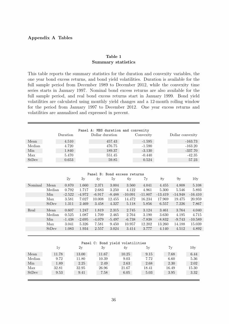
Appendix A Tables

Table 1

Summary statistics

This table reports the summary statistics for the duration and convexity variables, theone year bond excess returns, and bond yield volatilities. Duration is available for thefull sample period from December 1989 to December 2012, while the convexity timeseries starts in January 1997. Nominal bond excess returns are also available for thefull sample period, and real bond excess returns start in January 1999. Bond yieldvolatilities are calculated using monthly yield changes and a 12-month rolling windowfor the period from January 1997 to December 2012. One year excess returns andvolatilities are annualized and expressed in percent.

Panel A: MBS duration and convexity

Duration Dollar duration Convexity Dollar convexity

Mean 4.510 457.43 -1.595 -163.73Median 4.720 476.75 -1.590 -163.20Min 1.840 189.37 -3.130 -337.70Max 5.470 551.45 -0.440 -42.35StDev 0.653 59.85 0.524 57.23

Panel B: Bond excess returns

2y 3y 4y 5y 6y 7y 8y 9y 10y

Nominal Mean 0.870 1.660 2.371 3.004 3.560 4.041 4.455 4.808 5.108Median 0.792 1.717 2.683 3.250 4.122 4.961 5.300 5.546 5.893Min -2.522 -4.972 -6.917 -8.488 -10.091 -11.807 -13.419 -14.948 -16.410Max 3.581 7.027 10.008 12.455 14.472 16.234 17.969 19.475 20.959StDev 1.311 2.469 3.458 4.327 5.118 5.856 6.557 7.226 7.867

Real Mean 0.607 1.247 1.819 2.315 2.745 3.124 3.461 3.764 4.040Median 0.525 1.087 1.709 2.465 2.764 3.190 3.630 4.195 4.715Min -1.438 -2.695 -4.079 -5.497 -6.738 -7.838 -8.832 -9.743 -10.589Max 3.041 5.326 7.581 9.450 10.957 12.202 13.260 14.188 15.039StDev 1.083 1.934 2.557 3.024 3.414 3.777 4.140 4.512 4.892

Panel C: Bond yield volatilities

1y 2y 3y 4y 5y 7y 10y

Mean 11.78 13.00 11.67 10.25 9.15 7.68 6.44Median 9.72 11.80 10.39 9.03 7.72 6.60 5.36Min 1.89 2.25 2.49 2.63 2.68 2.30 2.02Max 32.81 32.95 26.96 21.67 18.41 16.49 15.30StDev 9.53 9.41 7.58 6.05 5.03 3.95 3.32

36

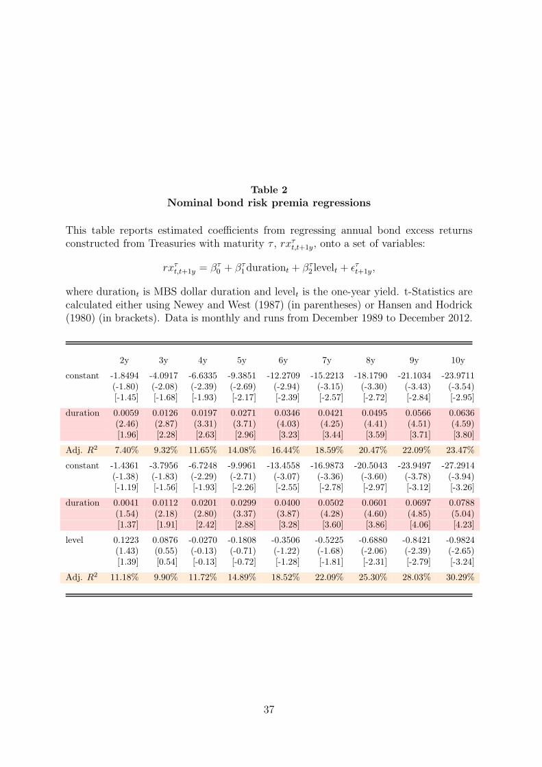
Table 2

Nominal bond risk premia regressions

This table reports estimated coefficients from regressing annual bond excess returnsconstructed from Treasuries with maturity τ , rxτ

t,t+1y, onto a set of variables:

rxτt,t+1y = βτ


2 levelt + ǫτt+1y,

where durationt is MBS dollar duration and levelt is the one-year yield. t-Statistics arecalculated either using Newey and West (1987) (in parentheses) or Hansen and Hodrick(1980) (in brackets). Data is monthly and runs from December 1989 to December 2012.

2y 3y 4y 5y 6y 7y 8y 9y 10y

constant -1.8494 -4.0917 -6.6335 -9.3851 -12.2709 -15.2213 -18.1790 -21.1034 -23.9711(-1.80) (-2.08) (-2.39) (-2.69) (-2.94) (-3.15) (-3.30) (-3.43) (-3.54)[-1.45] [-1.68] [-1.93) [-2.17] [-2.39] [-2.57] [-2.72] [-2.84] [-2.95]

duration 0.0059 0.0126 0.0197 0.0271 0.0346 0.0421 0.0495 0.0566 0.0636(2.46) (2.87) (3.31) (3.71) (4.03) (4.25) (4.41) (4.51) (4.59)[1.96] [2.28] [2.63] [2.96] [3.23] [3.44] [3.59] [3.71] [3.80]

Adj. R2 7.40% 9.32% 11.65% 14.08% 16.44% 18.59% 20.47% 22.09% 23.47%

constant -1.4361 -3.7956 -6.7248 -9.9961 -13.4558 -16.9873 -20.5043 -23.9497 -27.2914(-1.38) (-1.83) (-2.29) (-2.71) (-3.07) (-3.36) (-3.60) (-3.78) (-3.94)[-1.19] [-1.56] [-1.93] [-2.26] [-2.55] [-2.78] [-2.97] [-3.12] [-3.26]

duration 0.0041 0.0112 0.0201 0.0299 0.0400 0.0502 0.0601 0.0697 0.0788(1.54) (2.18) (2.80) (3.37) (3.87) (4.28) (4.60) (4.85) (5.04)[1.37] [1.91] [2.42] [2.88] [3.28] [3.60] [3.86] [4.06] [4.23]

level 0.1223 0.0876 -0.0270 -0.1808 -0.3506 -0.5225 -0.6880 -0.8421 -0.9824(1.43) (0.55) (-0.13) (-0.71) (-1.22) (-1.68) (-2.06) (-2.39) (-2.65)[1.39] [0.54] [-0.13] [-0.72] [-1.28] [-1.81] [-2.31] [-2.79] [-3.24]

Adj. R2 11.18% 9.90% 11.72% 14.89% 18.52% 22.09% 25.30% 28.03% 30.29%

37

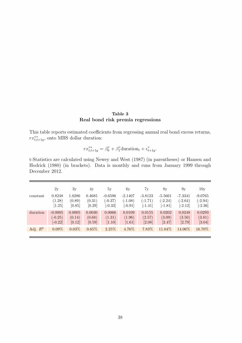
Table 3

Real bond risk premia regressions

This table reports estimated coefficients from regressing annual real bond excess returns,rxτ∗

t,t+1y, onto MBS dollar duration:

rxτ∗t,t+1y = βτ

0 + βτ1durationt + ǫτt+1y .

t-Statistics are calculated using Newey and West (1987) (in parentheses) or Hansen andHodrick (1980) (in brackets). Data is monthly and runs from January 1999 throughDecember 2012.

2y 3y 4y 5y 6y 7y 8y 9y 10y

constant 0.8248 1.0286 0.4685 -0.6596 -2.1407 -3.8123 -5.5661 -7.3341 -9.0765(1.28) (0.89) (0.31) (-0.37) (-1.08) (-1.71) (-2.24) (-2.64) (-2.94)[1.25] [0.85] [0.29] [-0.33] [-0.91] [-1.41] [-1.81] [-2.12] [-2.36]

duration -0.0005 0.0005 0.0030 0.0066 0.0109 0.0155 0.0202 0.0248 0.0293(-0.25) (0.14) (0.68) (1.31) (1.96) (2.57) (3.09) (3.50) (3.81)[-0.22] [0.12] [0.59] [1.10] [1.61] [2.08] [2.47] [2.79] [3.04]

Adj. R2 0.09% 0.03% 0.65% 2.25% 4.76% 7.83% 11.04% 14.06% 16.70%

38

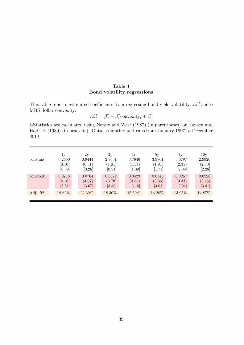
Table 4

Bond volatility regressions

This table reports estimated coefficients from regressing bond yield volatility, volτt , ontoMBS dollar convexity:


1 convexityt + ǫτt .

t-Statistics are calculated using Newey and West (1987) (in parentheses) or Hansen andHodrick (1980) (in brackets). Data is monthly and runs from January 1997 to December2012.

1y 2y 3y 4y 5y 7y 10yconstant 0.2650 0.9444 2.8631 3.7640 3.9861 3.6797 2.9920

(0.10) (0.31) (1.01) (1.54) (1.91) (2.35) (2.60)[0.09] [0.28] [0.91] [1.39] [1.71] [2.09] [2.28]

convexity 0.0713 0.0764 0.0572 0.0429 0.0345 0.0267 0.0226(4.18) (4.07) (3.78) (3.52) (3.36) (3.33) (3.45)[3.81] [3.67] [3.40] [3.16] [3.01] [2.94] [3.01]

Adj. R2 19.62% 22.30% 18.30% 15.59% 14.28% 13.95% 14.87%

39

Table 5

Regressions with Fed holdings

This table reports estimated coefficients from the following regression:

rxτt,t+1y = βτ


2 fed sharet + βτ3durationt × fed sharet + ǫτt,t+1y ,

where fed sharet is the Federal Reserve’s share of total MBS holdings. t-Statistics arecalculated using Newey and West (1987) (in parentheses) or Hansen and Hodrick (1980)(in brackets). Data is monthly and runs from January 2009 to December 2014.

2y 3y 4y 5y 7y 10yconstant -0.7857 -2.5375 -5.3436 -9.0014 -17.6518 -30.5812

(-2.36) (-2.70) (-2.85) (-2.97) (-3.26) (-3.71)[-2.05] [-2.36] [-2.48] [-2.57] [-2.79] [-3.17]

duration 0.0050 0.0141 0.0265 0.0409 0.0713 0.1116(4.30) (4.38) (4.27) (4.17) (4.15) (4.33)[3.67] [3.81] [3.73] [3.63] [3.60] [3.76]

interaction -0.0294 -0.0770 -0.1368 -0.1982 -0.3044 -0.4040(-4.68) (-4.11) (-3.69) (-3.41) (-3.10) (-2.88)[-3.92] [-3.55] [-3.20] [-2.96] [-2.70] [-2.55]

Adj. R2 43.84% 49.59% 50.45% 50.29% 51.72% 56.39%

constant -0.3602 -3.0718 -7.4939 -12.6500 -22.6729 -33.8161(-0.90) (-2.86) (-3.61) (-3.86) (-3.99) (-3.94)[-0.75] [-2.67] [-3.64] [-4.00] [-4.12] [-3.96]

duration 0.0040 0.0153 0.0313 0.0491 0.0824 0.1188(3.01) (4.47) (4.98) (5.07) (4.96) (4.72)[2.48] [3.93] [4.64] [4.84] [4.77] [4.46]

fed share -6.9698 8.7520 35.2216 59.7625 82.2438 52.9861(-1.24) (0.50) (0.98) (1.04) (0.81) (0.35)[-1.03] [0.45] [0.91] [0.97] [0.76] [0.33]

interaction -0.0145 -0.0958 -0.2122 -0.3262 -0.4805 -0.5175(-1.08) (-2.47) (-2.77) (-2.69) (-2.28) (-1.64)[-0.88] [-2.18] [-2.59] [-2.57] [-2.20] [-1.57]

Adj. R2 45.81% 50.74% 52.66% 52.76% 53.61% 57.54%

40

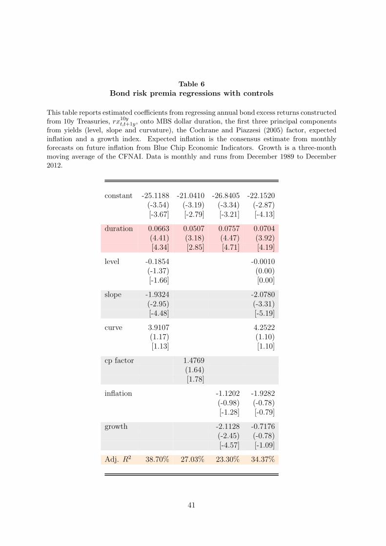
Table 6

Bond risk premia regressions with controls

This table reports estimated coefficients from regressing annual bond excess returns constructedfrom 10y Treasuries, rx10yt,t+1y, onto MBS dollar duration, the first three principal componentsfrom yields (level, slope and curvature), the Cochrane and Piazzesi (2005) factor, expectedinflation and a growth index. Expected inflation is the consensus estimate from monthlyforecasts on future inflation from Blue Chip Economic Indicators. Growth is a three-monthmoving average of the CFNAI. Data is monthly and runs from December 1989 to December2012.

constant -25.1188 -21.0410 -26.8405 -22.1520(-3.54) (-3.19) (-3.34) (-2.87)[-3.67] [-2.79] [-3.21] [-4.13]

duration 0.0663 0.0507 0.0757 0.0704(4.41) (3.18) (4.47) (3.92)[4.34] [2.85] [4.71] [4.19]

level -0.1854 -0.0010(-1.37) (0.00)[-1.66] [0.00]

slope -1.9324 -2.0780(-2.95) (-3.31)[-4.48] [-5.19]

curve 3.9107 4.2522(1.17) (1.10)[1.13] [1.10]

cp factor 1.4769(1.64)[1.78]

inflation -1.1202 -1.9282(-0.98) (-0.78)[-1.28] [-0.79]

growth -2.1128 -0.7176(-2.45) (-0.78)[-4.57] [-1.09]

Adj. R2 38.70% 27.03% 23.30% 34.37%

41

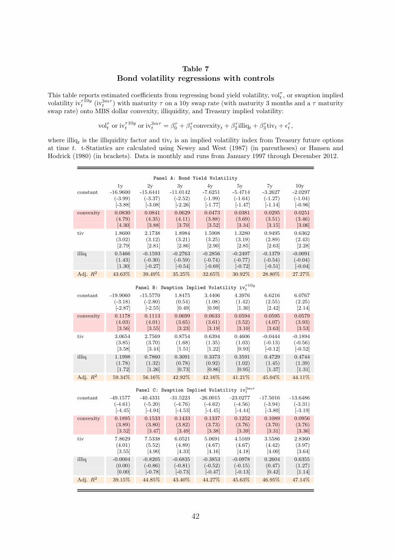
Table 7

Bond volatility regressions with controls

This table reports estimated coefficients from regressing bond yield volatility, volτt , or swaption impliedvolatility ivτ10yt (iv3mτ

t ) with maturity τ on a 10y swap rate (with maturity 3 months and a τ maturityswap rate) onto MBS dollar convexity, illiquidity, and Treasury implied volatility:

volτt or ivτ10yt or iv3mτt = βτ

0+ βτ

1convexityt + βτ

2illiqt + βτ

3tivt + ǫτt ,

where illiqt is the illiquidity factor and tivt is an implied volatility index from Treasury future optionsat time t. t-Statistics are calculated using Newey and West (1987) (in parentheses) or Hansen andHodrick (1980) (in brackets). Data is monthly and runs from January 1997 through December 2012.

Panel A: Bond Yield Volatility

1y 2y 3y 4y 5y 7y 10yconstant -16.9600 -15.6441 -11.0142 -7.6251 -5.4714 -3.2627 -2.0297

(-3.99) (-3.37) (-2.52) (-1.99) (-1.64) (-1.27) (-1.04)[-3.88] [-3.08] [-2.26] [-1.77] [-1.47] [-1.14] [-0.96]

convexity 0.0830 0.0841 0.0629 0.0473 0.0381 0.0295 0.0251(4.79) (4.35) (4.11) (3.88) (3.69) (3.51) (3.46)[4.30] [3.88] [3.70] [3.52] [3.34] [3.15] [3.06]

tiv 1.8600 2.1738 1.8984 1.5908 1.3280 0.9495 0.6362(3.02) (3.12) (3.21) (3.25) (3.19) (2.89) (2.43)[2.79] [2.81] [2.86] [2.90] [2.85] [2.63] [2.28]

illiq 0.5466 -0.1593 -0.2763 -0.2856 -0.2497 -0.1379 -0.0091(1.43) (-0.30) (-0.59) (-0.74) (-0.77) (-0.54) (-0.04)[1.30] [-0.27] [-0.54] [-0.69] [-0.72] [-0.51] [-0.04]

Adj. R2 43.63% 39.49% 35.25% 32.65% 30.92% 28.80% 27.27%

Panel B: Swaption Implied Volatility ivτ10yt

constant -19.9060 -15.5770 1.8475 3.4406 4.3976 6.6216 6.0767(-3.18) (-2.80) (0.54) (1.08) (1.42) (2.55) (2.25)[-2.87] [-2.55] [0.49] [0.99] [1.30] [2.42] [2.14]

convexity 0.1178 0.1113 0.0699 0.0633 0.0594 0.0595 0.0579(4.03) (4.01) (3.65) (3.61) (3.52) (4.07) (3.93)[3.56] [3.55] [3.23] [3.19] [3.10] [3.63] [3.53]

tiv 3.0654 2.7569 0.8754 0.6394 0.4606 -0.0444 -0.1894(3.85) (3.70) (1.68) (1.35) (1.03) (-0.13) (-0.56)[3.58] [3.44] [1.51] [1.22] [0.93] [-0.12] [-0.52]

illiq 1.1998 0.7860 0.3091 0.3373 0.3591 0.4729 0.4744(1.78) (1.32) (0.78) (0.92) (1.02) (1.45) (1.39)[1.72] [1.26] [0.73] [0.86] [0.95] [1.37] [1.31]

Adj. R2 59.34% 56.16% 42.92% 42.16% 41.21% 45.04% 44.11%

Panel C: Swaption Implied Volatility iv3mτt

constant -49.1577 -40.4331 -31.5223 -26.0015 -23.0277 -17.5016 -13.6486(-4.61) (-5.20) (-4.76) (-4.62) (-4.56) (-3.94) (-3.31)[-4.45] [-4.94] [-4.53] [-4.45] [-4.44] [-3.80] [-3.19]

convexity 0.1895 0.1533 0.1433 0.1337 0.1252 0.1089 0.0956(3.89) (3.80) (3.82) (3.73) (3.76) (3.70) (3.76)[3.52] [3.47] [3.49] [3.38] [3.39] [3.31] [3.36]

tiv 7.8629 7.5338 6.0521 5.0691 4.5169 3.5586 2.8360(4.01) (5.52) (4.89) (4.67) (4.67) (4.42) (3.97)[3.55] [4.90] [4.33] [4.16] [4.18] [4.00] [3.64]

illiq -0.0004 -0.8205 -0.6835 -0.3853 -0.0978 0.2604 0.6355(0.00) (-0.86) (-0.81) (-0.52) (-0.15) (0.47) (1.27)[0.00] [-0.78] [-0.73] [-0.47] [-0.13] [0.42] [1.14]

Adj. R2 39.15% 44.85% 43.40% 44.27% 45.63% 46.95% 47.14%

42

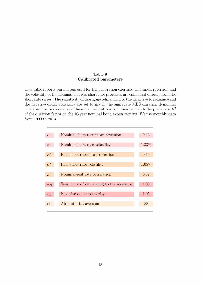
Table 8

Calibrated parameters

This table reports parameters used for the calibration exercise. The mean reversion andthe volatility of the nominal and real short rate processes are estimated directly from theshort rate series. The sensitivity of mortgage refinancing to the incentive to refinance andthe negative dollar convexity are set to match the aggregate MBS duration dynamics.The absolute risk aversion of financial institutions is chosen to match the predictive R2

of the duration factor on the 10-year nominal bond excess returns. We use monthly datafrom 1990 to 2013.

κ Nominal short rate mean reversion 0.13

σ Nominal short rate volatility 1.33%

κ∗ Real short rate mean reversion 0.16

σ∗ Real short rate volatility 1.05%

ρ Nominal-real rate correlation 0.87

κD Sensitivity of refinancing to the incentive 1.05

ηy Negative dollar convexity 1.05

α Absolute risk aversion 88

43

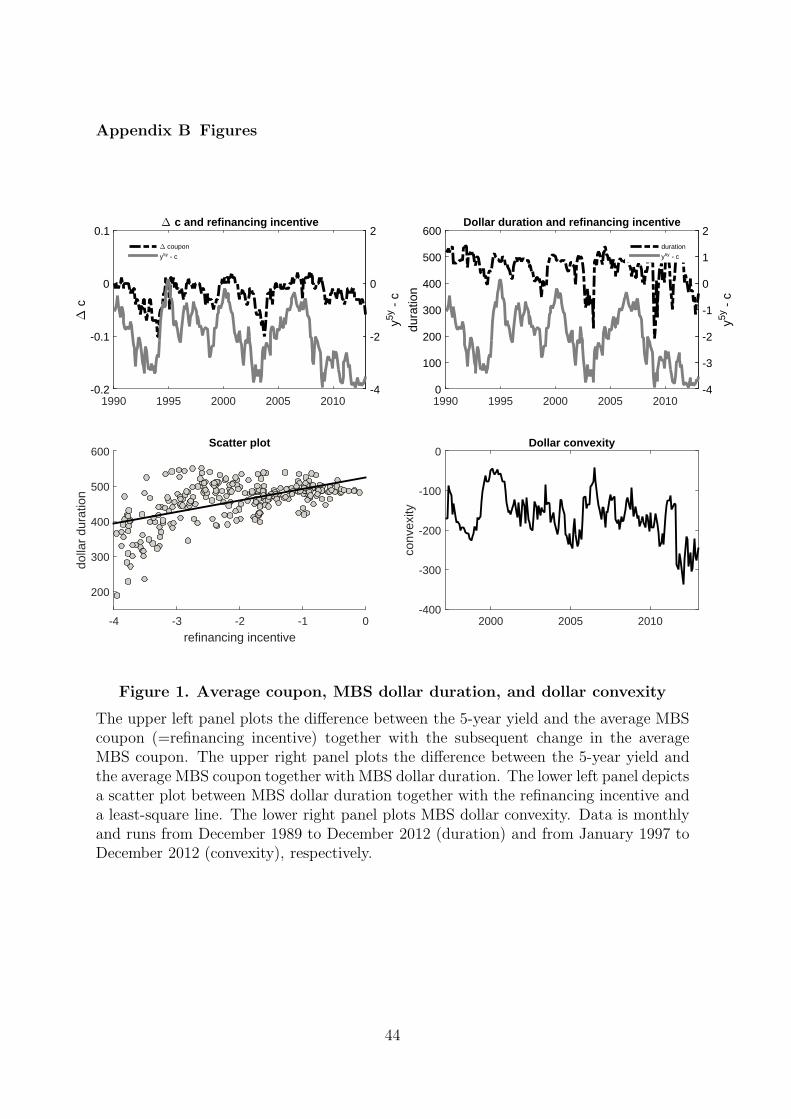
Appendix B Figures

1990 1995 2000 2005 2010

∆ c

-0.2

-0.1

0

0.1∆ c and refinancing incentive

y5y -

c-4

-2

0

2∆ coupon

y5y - c

1990 1995 2000 2005 2010du

ratio

n

0

100

200

300

400

500

600Dollar duration and refinancing incentive

y5y -

c

-4

-3

-2

-1

0

1

2duration

y5y - c

refinancing incentive-4 -3 -2 -1 0

dolla

r du

ratio

n

200

300

400

500

600Scatter plot

2000 2005 2010

conv

exity

-400

-300

-200

-100

0Dollar convexity

Figure 1. Average coupon, MBS dollar duration, and dollar convexity

The upper left panel plots the difference between the 5-year yield and the average MBScoupon (=refinancing incentive) together with the subsequent change in the averageMBS coupon. The upper right panel plots the difference between the 5-year yield andthe average MBS coupon together with MBS dollar duration. The lower left panel depictsa scatter plot between MBS dollar duration together with the refinancing incentive anda least-square line. The lower right panel plots MBS dollar convexity. Data is monthlyand runs from December 1989 to December 2012 (duration) and from January 1997 toDecember 2012 (convexity), respectively.

44

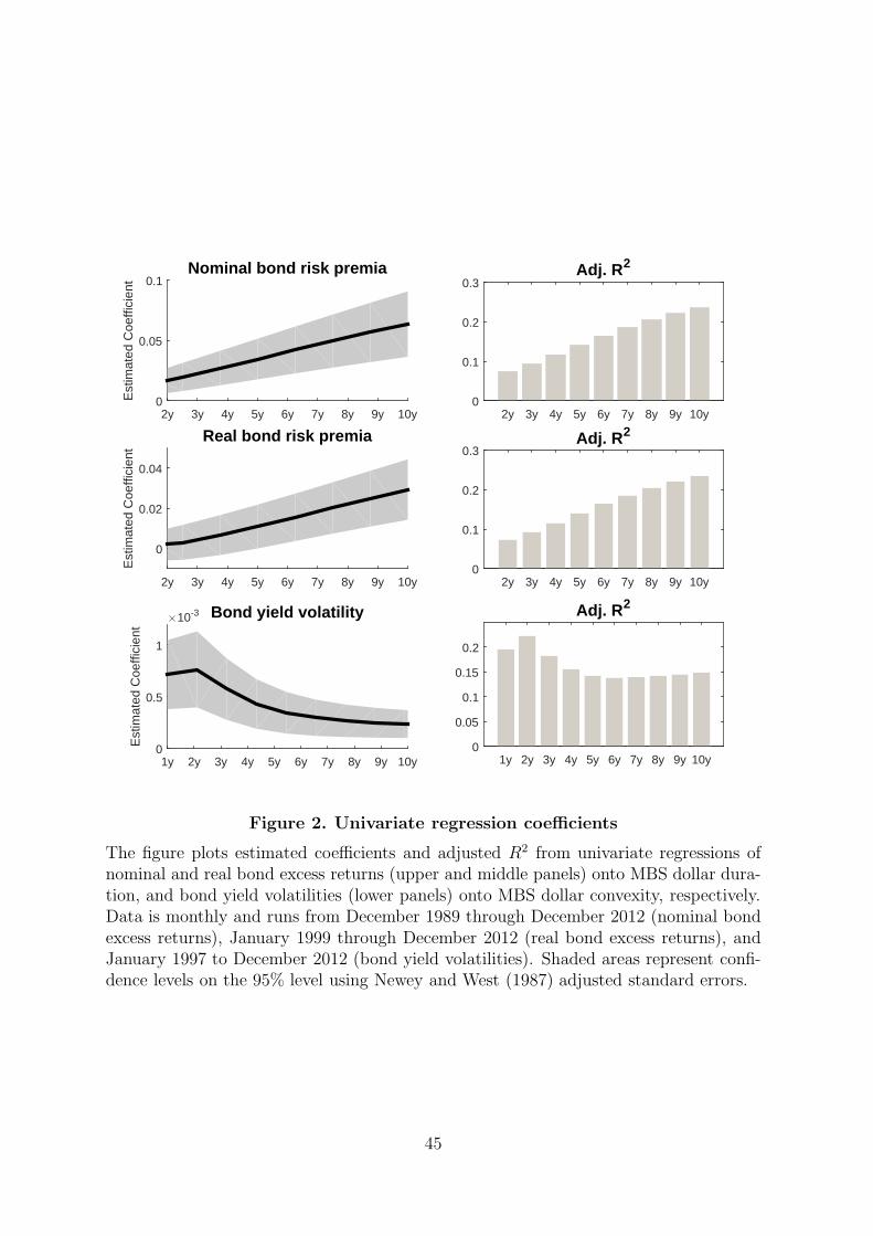
2y 3y 4y 5y 6y 7y 8y 9y 10y

Est

imat

ed C

oeffi

cien

t

0

0.05

0.1Nominal bond risk premia

2y 3y 4y 5y 6y 7y 8y 9y 10y0

0.1

0.2

0.3Adj. R2

2y 3y 4y 5y 6y 7y 8y 9y 10y

Est

imat

ed C

oeffi

cien

t

0

0.02

0.04

Real bond risk premia

2y 3y 4y 5y 6y 7y 8y 9y 10y0

0.1

0.2

0.3Adj. R2

1y 2y 3y 4y 5y 6y 7y 8y 9y 10y

Est

imat

ed C

oeffi

cien

t

×10-3

0

0.5

1

Bond yield volatility

1y 2y 3y 4y 5y 6y 7y 8y 9y 10y0

0.05

0.1

0.15

0.2

Adj. R2

Figure 2. Univariate regression coefficients

The figure plots estimated coefficients and adjusted R2 from univariate regressions ofnominal and real bond excess returns (upper and middle panels) onto MBS dollar dura-tion, and bond yield volatilities (lower panels) onto MBS dollar convexity, respectively.Data is monthly and runs from December 1989 through December 2012 (nominal bondexcess returns), January 1999 through December 2012 (real bond excess returns), andJanuary 1997 to December 2012 (bond yield volatilities). Shaded areas represent confi-dence levels on the 95% level using Newey and West (1987) adjusted standard errors.

45

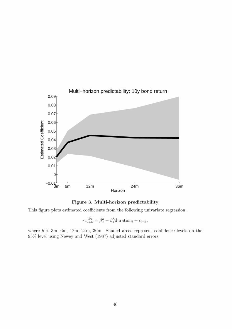
3m 6m 12m 24m 36m−0.01

0

0.01

0.02

0.03

0.04

0.05

0.06

0.07

0.08

0.09Multi−horizon predictability: 10y bond return

Est

imat

ed C

oeffi

cien

t

Horizon

Figure 3. Multi-horizon predictability

This figure plots estimated coefficients from the following univariate regression:

rx10yt+h = βh

0 + βh1durationt + ǫt+h,

where h is 3m, 6m, 12m, 24m, 36m. Shaded areas represent confidence levels on the95% level using Newey and West (1987) adjusted standard errors.

46

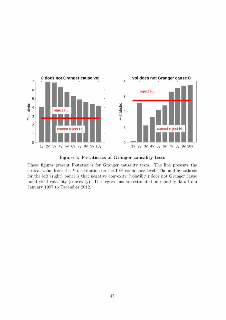
1y 2y 3y 4y 5y 6y 7y 8y 9y 10y

F-s

tatis

tic

0

1

2

3

4

5

6

7C does not Granger cause vol

1y 2y 3y 4y 5y 6y 7y 8y 9y 10y

F-s

tatis

tic

0

1

2

3

4vol does not Granger cause C

reject H0

reject H0

cannot reject H0

cannot reject H0

Figure 4. F-statistics of Granger causality tests

These figures present F-statistics for Granger causality tests. The line presents thecritical value from the F -distribution on the 10% confidence level. The null hypothesisfor the left (right) panel is that negative convexity (volatility) does not Granger causebond yield volatility (convexity). The regressions are estimated on monthly data fromJanuary 1997 to December 2012.

47

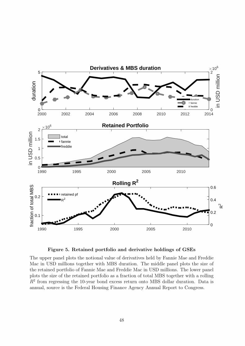
1990 1995 2000 2005 2010

frac

tion

of to

tal M

BS

0.1

0.2

Rolling R2

R2

0

0.2

0.4

0.6

retained pf

R2

1990 1995 2000 2005 2010

in U

SD

mill

ion

×106

0

0.5

1

1.5

2Retained Portfolio

totalfanniefreddie

2000 2002 2004 2006 2008 2010 2012 2014

dura

tion

0

5Derivatives & MBS duration

in U

SD

mill

ion

×106

0

2

duration

fannie

freddie

Figure 5. Retained portfolio and derivative holdings of GSEs

The upper panel plots the notional value of derivatives held by Fannie Mae and FreddieMac in USD millions together with MBS duration. The middle panel plots the size ofthe retained portfolio of Fannie Mae and Freddie Mac in USD millions. The lower panelplots the size of the retained portfolio as a fraction of total MBS together with a rollingR2 from regressing the 10-year bond excess return onto MBS dollar duration. Data isannual, source is the Federal Housing Finance Agency Annual Report to Congress.

48

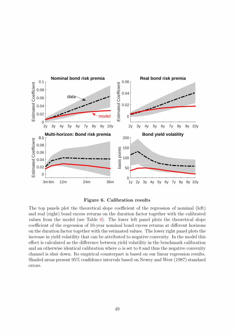
2y 3y 4y 5y 6y 7y 8y 9y 10y

Est

imat

ed C

oeffi

cien

t

0

0.02

0.04

0.06

0.08

0.1Nominal bond risk premia

2y 3y 4y 5y 6y 7y 8y 9y 10y

Est

imat

ed C

oeffi

cien

t0

0.02

0.04

0.06Real bond risk premia

3m 6m 12m 24m 36m

Est

imat

ed C

oeffi

cien

t

0

0.02

0.04

0.06

0.08

0.10.1Multi-horizon: Bond risk premia

1y 2y 3y 4y 5y 6y 7y 8y 9y 10y

basi

s po

ints

0

50

100

150

200Bond yield volatility

model

data

Figure 6. Calibration results

The top panels plot the theoretical slope coefficient of the regression of nominal (left)and real (right) bond excess returns on the duration factor together with the calibratedvalues from the model (see Table 8). The lower left panel plots the theoretical slopecoefficient of the regression of 10-year nominal bond excess returns at different horizonson the duration factor together with the estimated values. The lower right panel plots theincrease in yield volatility that can be attributed to negative convexity. In the model thiseffect is calculated as the difference between yield volatility in the benchmark calibrationand an otherwise identical calibration where α is set to 0 and thus the negative convexitychannel is shut down. Its empirical counterpart is based on our linear regression results.Shaded areas present 95% confidence intervals based on Newey andWest (1987) standarderrors.

49

All volumes are available on our website www.bis.org.

Previous volumes in this series

No Title Author

531 December 2015

The supply side of household finance Gabriele Foà, Leonardo Gambacorta, Luigi Guiso and Paolo Emilio Mistrulli

530 November 2015

Commercial Bank Failures During The Great Recession: The Real (Estate) Story

Adonis Antoniades

529 November 2015

A search-based model of the interbank money market and monetary policy implementation

Morten Bech and Cyril Monnet

528 November 2015

External shocks, banks and optimal monetary policy in an open economy

Yasin Mimir and Enes Sunel

527 November 2015

Expectations and Risk Premia at 8:30AM: Macroeconomic Announcements and the Yield Curve

Peter Hördahl, Eli M Remolona and Giorgio Valente

526 November 2015

Modelling the Time-Variation in Euro Area Lending Spread

Boris Blagov, Michael Funke and Richhild Moessner

525 October 2015

Capital flows and the current account: Taking financing (more) seriously

Claudio Borio and Piti Disyatat

524 October 2015

Breaking free of the triple coincidence in international finance

Stefan Avdjiev, Robert N McCauley and Hyun Song Shin

523 October 2015

The evolution of inflation expectations in Canada and the US

James Yetman

522 October 2015

Do banks extract informational rents through collateral?

Bing Xu, Honglin Wang and Adrian van Rixtel

521 October 2015

Does variance risk have two prices? Evidence from the equity and option markets

Laurent Barras and Aytek Malkhozov

520 October 2015

Optimal Inflation with Corporate Taxation and Financial Constraints

Daria Finocchiaro, Giovanni Lombardo, Caterina Mendicino and Philippe Weil

519 October 2015

The hunt for duration: not waving but drowning?

Dietrich Domanski, Hyun Song Shin and Vladyslav Sushko

518 October 2015

Monetary Policy and Financial Spillovers: Losing Traction?

Piti Disyatat and Phurichai Rungcharoenkitkul

517 October 2015

Leverage on the buy side Fernando Avalos, Ramon Moreno and Tania Romero

516 October 2015

Optimal Time-Consistent Macroprudential Policy

Javier Bianchi and Enrique G. Mendoza

515 October 2015

The impact of CCPs' margin policies on repo markets

Arianna Miglietta, Cristina Picillo and Mario Pietrunti

514 September 2015

The influence of monetary policy on bank profitability

Claudio Borio, Leonardo Gambacorta and Boris Hofmann

Documents

BIS Working Papers · BIS Working Papers are written by members of the ... Mortgage-backed securities (MBS) ... supply driven by mortgage debt and the risk-bearing …