Embed Size (px)
Citation preview
BIS Working PapersNo 432
Liquidity regulation and the implementation of monetary policy by Morten L. Bech and Todd Keister
Monetary and Economic Department
October 2013
JEL classification: E43, E52, E58, G28.
Keywords: Basel III, Liquidity regulation, LCR, Reserves, Corridor system, Monetary policy.
BIS Working Papers are written by members of the Monetary and Economic Department of the Bank for International Settlements, and from time to time by other economists, and are published by the Bank. The papers are on subjects of topical interest and are technical in character. The views expressed in them are those of their authors and not necessarily the views of the BIS.
This publication is available on the BIS website (www.bis.org).
© Bank for International Settlements 2013. All rights reserved. Brief excerpts may be reproduced or translated provided the source is stated.
ISSN 1020-0959 (print)
ISBN 1682-7678 (online)

Liquidity regulation and the implementation of monetary policy∗
Morten L. Bech
Bank for International Settlements
Todd Keister
Rutgers University
October 9, 2013
Abstract
In addition to revamping existing rules for bank capital, Basel III introduces a new global frame-
work for liquidity regulation. One part of this framework is the liquidity coverage ratio (LCR),
which requires banks to hold sufficient high-quality liquid assets to survive a 30-day period of
market stress. As monetary policy typically involves targeting the interest rate on loans of one
of these assets — central bank reserves — it is important to understand how this regulation may
impact the efficacy of central banks’ current operational frameworks. We introduce term funding
and an LCR requirement into an otherwise standard model of monetary policy implementation.
Our model shows that if banks face the possibility of an LCR shortfall, then the usual link
between open market operations and the overnight interest rate changes and the short end of
the yield curve becomes steeper. Our results suggest that central banks may want to adjust
their operational frameworks as the new regulation is implemented.
JEL classification: E43, E52, E58, G28.
Keywords: Basel III, Liquidity regulation, LCR, Reserves, Corridor system, Monetary policy.
∗We thank Stephen Cecchetti, Andrew Filardo, Jamie McAndrews, Cyril Monnet, William Nelson, Jeremy Stein,
participants at the ECB Workshop on “Excess Liquidity and Money Market Functioning” and at the 2012 Joint
Central Banker’s Conference, as well as seminar participants at the BIS, Danmarks Nationalbank, and the Federal
Reserve Board for helpful comments. The views expressed herein are those of the authors and do not necessarily
reflect those of the Bank for International Settlements
1
1 Introduction
In response to the recent global financial crisis, the Basel Committee on Banking Supervision
(BCBS) announced a new international regulatory framework for banks, known as Basel III. In
addition to revamping the existing capital rules, Basel III introduces — for the first time — a global
framework for liquidity regulation. The new regulation prescribes two separate, but complementary,
minimum standards for managing liquidity risk: the liquidity coverage ratio (LCR) and the net
stable funding ratio (NSFR). These standards aim to ensure that banks hold a more liquid portfolio
of assets and better manage the maturity mismatch between their assets and liabilities. Specifically,
the LCR requires each bank to hold a sufficient quantity of highly-liquid assets to survive a 30-day
period of market stress. The NSFR focuses on a one-year time horizon and establishes a minimum
amount of stable funding each bank must obtain based on the liquidity characteristics of its assets
and activities. Implementation of the LCR and the NSFR is scheduled to begin in January 2015
and January 2018, respectively.1
How might these new liquidity regulations affect the process through which central banks im-
plement monetary policy? In many jurisdictions, this process involves setting a target for the
interest rate at which banks lend central bank reserves to one another, typically overnight and
on an unsecured basis. Because these reserves are part of banks’ portfolio of highly-liquid assets,
the regulations will potentially alter behavior in the interbank market, changing the relationship
between market conditions and the resulting interest rate. In addition, monetary policy operations
will influence banks’ regulatory liquidity ratios and, hence, may affect their compliance with the
new liquidity standards, at least at the margin. These linkages suggest that the new regulations
may have subtle consequences that could potentially have an impact on the effectiveness of central
banks’ current operating procedures.
We extend a standard model of banks’ reserve management and interbank lending to study how
the introduction of an LCR requirement affects the process of implementing monetary policy in a
1The LCR requirement will be phased in gradually, beginning at 60% coverage in January 2015 and rising 10
percentage points each year to reach 100% in January 2019.
2

corridor system. While there has been some discussion of this topic,2 ours is the first model that
can be used to analyze these issues systematically. We show that when banks face the possibility
of an LCR shortfall, the relationship between the quantity of central bank reserves and market
interest rates changes. A bank that is concerned about possibly violating the LCR has a stronger
incentive to seek term funding in the market and is more likely to borrow from the central bank’s
standing facility. Both of these actions add to the bank’s reserve holdings and thus lower the need
to seek funds in the overnight market to ensure the bank’s reserve requirement is met. This lower
demand for overnight funds tends to drive down the overnight rate, whereas the increased demand
for term funding tends to make the short end of the yield curve steeper.
We also study a central bank’s ability to control interest rates through open market operations.
We look at operations that differ along several dimensions: the types of assets used in the operation,
the types of counterparties, and outright versus reverse operations. In the standard model with
no LCR requirement, the overnight interest rate is determined by the total quantity of reserves
supplied by the central bank; the type of operation used to create these reserves is irrelevant. We
show that once an LCR requirement is introduced, this result no longer holds. In our model, the
structure of an open market operation determines its effects on bank balance sheets and, hence, the
likelihood that individual banks may face an LCR deficiency. This likelihood, in turn, affects banks’
incentives to trade in interbank markets. As a result, the impact of an operation on equilibrium
interest rates can be sensitive to the way it is structured. For example, in some cases the overnight
rate is more responsive to changes in the supply of reserves than in the standard model, while
in some cases it becomes unresponsive. In other cases the yield curve tends to steepen when the
central bank adds reserves, while in others it steepens when reserves are removed. The size of these
effects depends on a variety of factors, including the liquidity surplus/deficit of the banking system
and the specific parameters used in calculating the LCR requirement.
The LCR rules were first published in December 2010, but were subsequently revised in January
2013. Our model suggests that the revised rules mitigate — but do not eliminate — the regulation’s
impact on monetary policy implementation. Overall, our results indicate that central banks may
2See, for example, Bindseil and Lamoot (2011) and Schmidt (2012). Bonner and Eijffinger (2013) study empirically
the impact of the quantitative liquidity requirement introduced in Holland in 2003 on money markets there.
3

wish to adjust their operational frameworks for implementing monetary policy when the LCR is
introduced. At a minimum, they will need to monitor developments that materially affect the LCR
of the banking system, in much the same way as they have traditionally monitored other factors
that affect interbank markets.
We briefly review the LCR regulation in the next section before presenting our model in Section
3. We derive banks’ demand for overnight and term interbank loans as well as the equilibrium
interest rates on these loans in Section 4, while in Section 5 we study the central bank’s ability
to control interest rates using open market operations. Section 6 examines the importance of the
treatment of central bank loans in the LCR calculation and discusses the impact of the revised
LCR rules. Section 7 concludes with a discussion of policy options.
2 The liquidity coverage ratio (LCR)
The liquidity coverage ratio is calculated by dividing a bank’s stock of unencumbered high-quality
liquid assets (HQLA) by its projected net cash outflows over a 30-day horizon under a stress scenario
specified by supervisors. The new regulation requires this ratio to be at least one, that is,
=Stock of unencumbered high-quality liquid assets
Total net cash outflows over the next 30 calendar days≥ 1 (1)
Two types (or “levels”) of assets can be applied toward the HQLA pool. Level 1 assets include cash,
central bank reserves and certain marketable securities backed by sovereigns and central banks.3
Level 2 assets are divided into two subgroups: Level 2A assets include certain government securities,
corporate debt securities and covered bonds, while Level 2B assets include lower-rated corporate
bonds, residential mortgage backed securities and equities that meet certain conditions. Level 2A
assets can account for a maximum of 40% of a bank’s total stock of HQLA, whereas Level 2B assets
can account for a maximum of 15% of the total.
3Central bank reserves held to meet reserve requirements may be included in the calculation of HQLA under
some conditions. Specifically, BCBS (2013) states that “[l]ocal supervisors should discuss and agree with the relevant
central bank the extent to which central bank reserves should count towards the stock of liquid assets, i.e., the extent
to which reserves are able to be drawn down in times of stress”.
4

The denominator of the LCR, projected net cash outflows, is calculated by multiplying the size
of various types of liabilities and off-balance sheet commitments by the rates at which they are
expected to run off or be drawn down in the stress scenario. This scenario includes a partial loss
of retail deposits, significant loss of unsecured and secured wholesale funding, contractual outflows
from derivative positions associated with a three-notch ratings downgrade, and substantial calls on
off-balance sheet exposures. The calibration of scenario run-off rates reflects a combination of the
experience during the recent financial crisis, internal stress scenarios of banks, and existing regu-
latory and supervisory standards. From these outflows, banks are permitted to subtract expected
inflows for 30 calendar days into the future. To prevent banks from relying solely on anticipated
inflows to meet their liquidity requirement, and to ensure a minimum level of liquid asset holdings,
the fraction of outflows that can be offset this way is capped at 75%.
Once the LCR has been fully implemented, its 100% threshold will be a minimum requirement
in normal times. During a period of stress, however, banks would be expected to use their pool of
liquid assets, thereby temporarily falling below the required level. Our focus in this paper is on the
process of implementing monetary policy in normal times, when banks are expected to fully meet
the requirement.
3 The model
Our analysis is based on a model of monetary policy implementation in the tradition of Poole
(1968).4 Banks raise capital and issue deposits while holding loans, bonds and reserves as assets.
They can borrow and lend funds in interbank markets for overnight and term loans, and they
are subject to both a reserve requirement and the LCR requirement discussed above. The central
bank influences activity in interbank markets using a combination of open market operations and
standing facilities where banks can deposit surplus funds or borrow against collateral.
4Contributions to this literature include Dotsey (1991), Clouse and Dow (1999, 2002), Guthrie and Wright (2000),
Bartolini, Bertola and Prati (2002), Bindseil (2004), Whitesell (2006), Ennis and Weinberg (2007), Ennis and Keister
(2008), Bech and Klee (2011), and Afonso and Lagos (2012), among others.
5
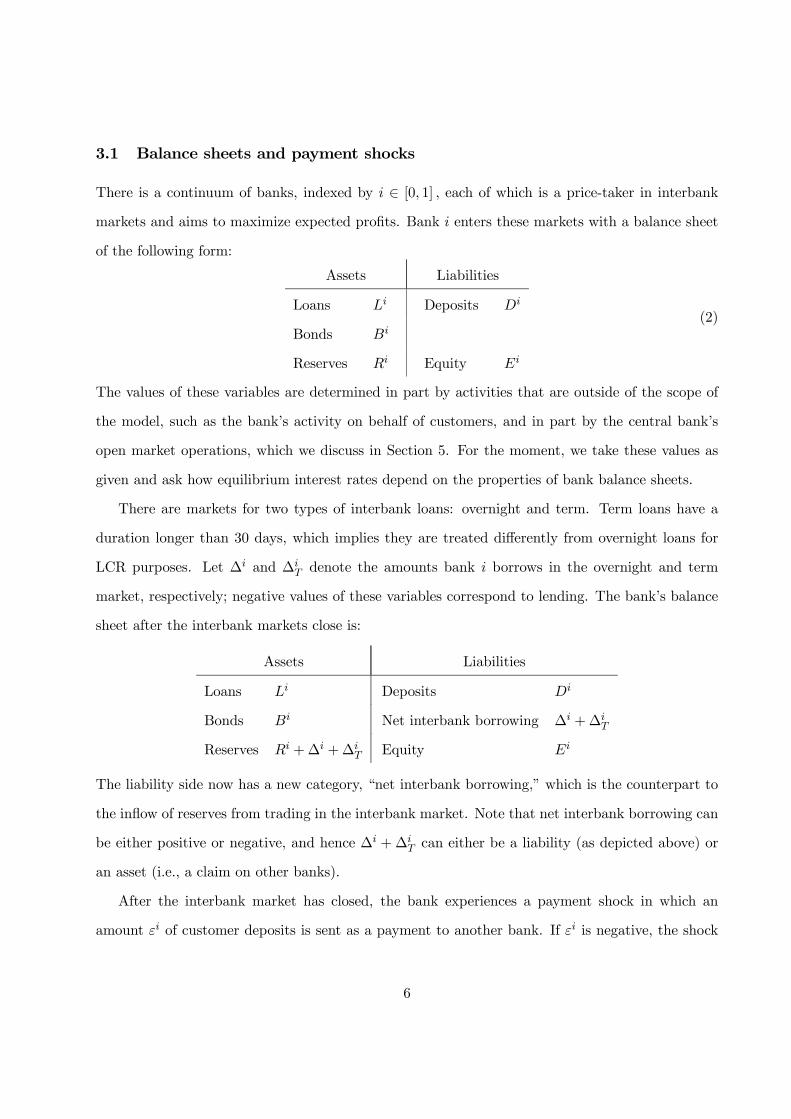
3.1 Balance sheets and payment shocks
There is a continuum of banks, indexed by ∈ [0 1] each of which is a price-taker in interbankmarkets and aims to maximize expected profits. Bank enters these markets with a balance sheet
of the following form:
Assets Liabilities
Loans Deposits
Bonds
Reserves Equity
(2)
The values of these variables are determined in part by activities that are outside of the scope of
the model, such as the bank’s activity on behalf of customers, and in part by the central bank’s
open market operations, which we discuss in Section 5. For the moment, we take these values as
given and ask how equilibrium interest rates depend on the properties of bank balance sheets.
There are markets for two types of interbank loans: overnight and term. Term loans have a
duration longer than 30 days, which implies they are treated differently from overnight loans for
LCR purposes. Let ∆ and ∆ denote the amounts bank borrows in the overnight and term
market, respectively; negative values of these variables correspond to lending. The bank’s balance
sheet after the interbank markets close is:
Assets Liabilities
Loans Deposits
Bonds Net interbank borrowing ∆ +∆
Reserves +∆ +∆ Equity
The liability side now has a new category, “net interbank borrowing,” which is the counterpart to
the inflow of reserves from trading in the interbank market. Note that net interbank borrowing can
be either positive or negative, and hence ∆ +∆ can either be a liability (as depicted above) or
an asset (i.e., a claim on other banks).
After the interbank market has closed, the bank experiences a payment shock in which an
amount of customer deposits is sent as a payment to another bank. If is negative, the shock
6
represents an unexpected inflow of funds. The value of for each bank is drawn from a common,
symmetric distribution with density function and with zero mean. The assumption that the
interbank market closes before these payment shocks are realized is a standard way of capturing
the imperfections in interbank markets that prevent banks from being able to exactly target their
end-of-day reserve balance.5 Depending on the size of its payment shock, the bank may need to
borrow from the central bank at the end of the day to meet its regulatory requirements. Let ≥ 0denote the amount borrowed by bank . The bank pledges loans to the central bank as collateral;
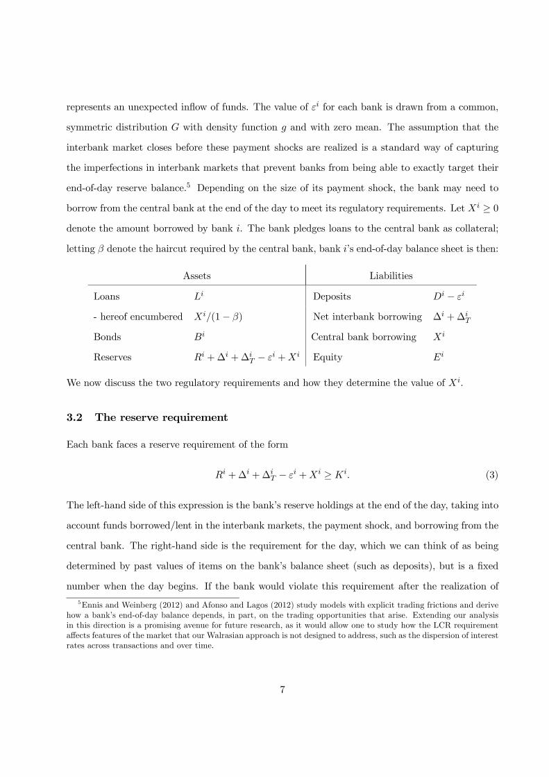
letting denote the haircut required by the central bank, bank ’s end-of-day balance sheet is then:
Assets Liabilities
Loans Deposits −
- hereof encumbered (1− ) Net interbank borrowing ∆ +∆
Bonds Central bank borrowing
Reserves +∆ +∆ − + Equity
We now discuss the two regulatory requirements and how they determine the value of
3.2 The reserve requirement
Each bank faces a reserve requirement of the form
+∆ +∆ − + ≥ (3)
The left-hand side of this expression is the bank’s reserve holdings at the end of the day, taking into
account funds borrowed/lent in the interbank markets, the payment shock, and borrowing from the
central bank. The right-hand side is the requirement for the day, which we can think of as being
determined by past values of items on the bank’s balance sheet (such as deposits), but is a fixed
number when the day begins. If the bank would violate this requirement after the realization of
5Ennis and Weinberg (2012) and Afonso and Lagos (2012) study models with explicit trading frictions and derive
how a bank’s end-of-day balance depends, in part, on the trading opportunities that arise. Extending our analysis
in this direction is a promising avenue for future research, as it would allow one to study how the LCR requirement
affects features of the market that our Walrasian approach is not designed to address, such as the dispersion of interest
rates across transactions and over time.
7
the payment shock, it must borrow funds from the central bank to ensure that (3) holds.
Borrowing from the central bank is costly and, therefore, each bank will borrow the minimum
amount needed to meet its regulatory requirements. Let denote the minimum amount bank
must borrow to fulfill the reserve requirement in (3), that is,
= max
© + − −∆ −∆
0ª (4)
3.3 The LCR requirement
In the context of our model, bank ’s LCR requirement is
= + +∆ +∆
− +
( − ) +∆ + ≥ 1 (5)
Recall from (1) that the numerator of the ratio is the total value of the bank’s high-quality liquid
assets, which here simply equals its end-of-day holdings of bonds plus reserves.6 The denominator
measures the 30-day net cash outflow assumed under the stress scenario, which includes the run-off
of deposits at rate , of overnight interbank loans at 100%, and of loans from the central bank
at rate . The LCR rules allow a run-off rate on (secured) loans from the central bank of 0%
but, as these rules are a minimum standard, local authorities can set a higher value of at their
discretion. Terms loans expire outside the duration of the stress scenario and hence do not enter
the denominator of the ratio.7
Let denote the minimum amount bank must borrow from the central bank to fulfill the
LCR requirement in (5), that is,
= max
½(1− )
− − −∆
1− 0
¾ (6)
where
≡ −
6For simplicity, we assume that reserves held to meet reserve requirements are included in the calculation of
high-quality liquid assets. It is straightforward to modify the model to exclude these balances.7The regulation divides retail deposits into two categories: “stable” and “less stable”. Stable retail deposits are
those covered by an effective deposit insurance scheme as defined in the LCR rules text and are assigned a minimum
run-off rate of 5%. Less stable retail deposits are assigned a minimum run-off rate of 10%. If the deposit insurance
scheme meets certain additional criteria, the run-off rate for stable deposits can be lowered to 3%. See BCBS (2013)
for more detail.
8
represents the bank’s surplus (or shortfall, if negative) of liquid assets for LCR purposes before
reserve holdings are taken into account.
3.4 Borrowing from the central bank
Combining equations (4) and (6), the minimum amount bank must borrow from the central bank’s
lending facility to meet both its reserve and LCR requirements is given by
= max©
ª(7)
= max
½ + − −∆ −∆
(1− )
− − −∆
1− 0
¾
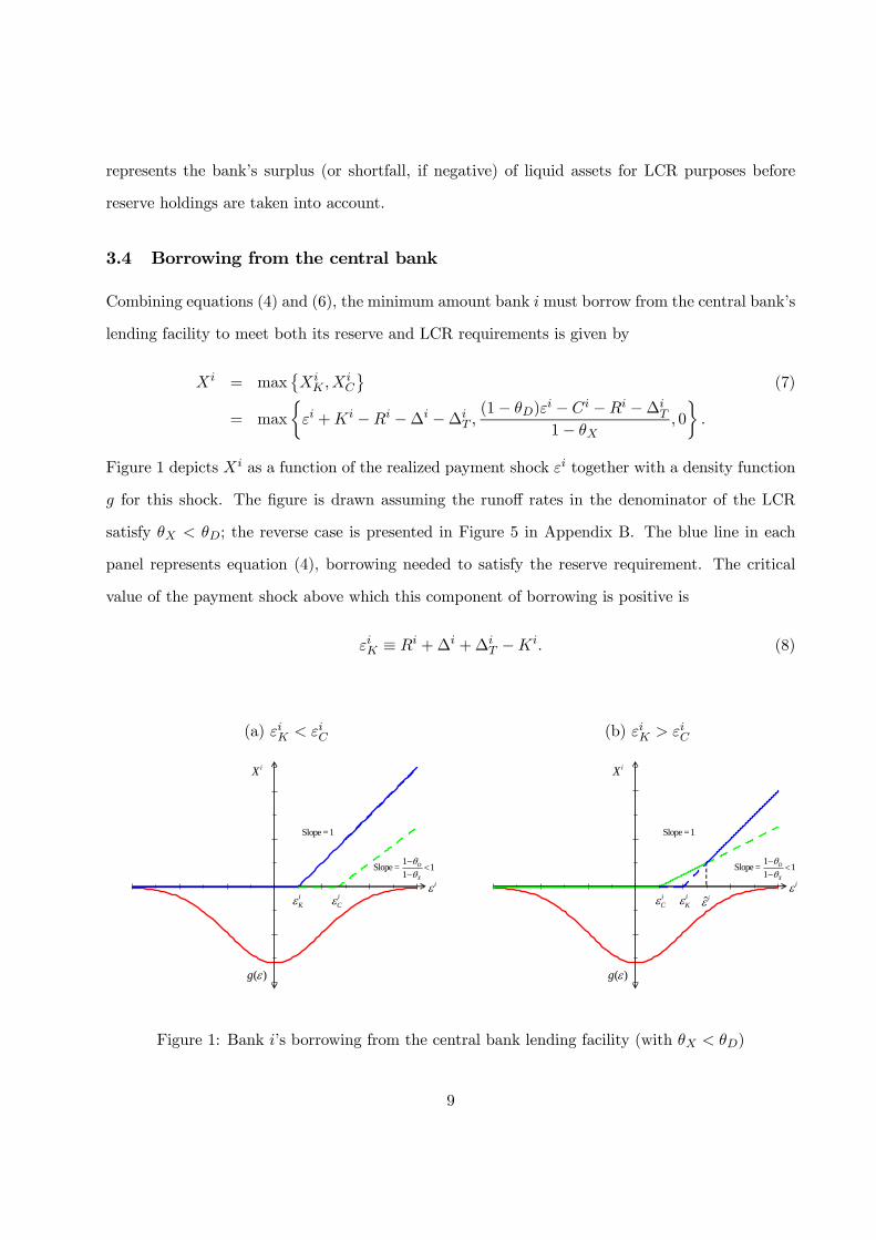
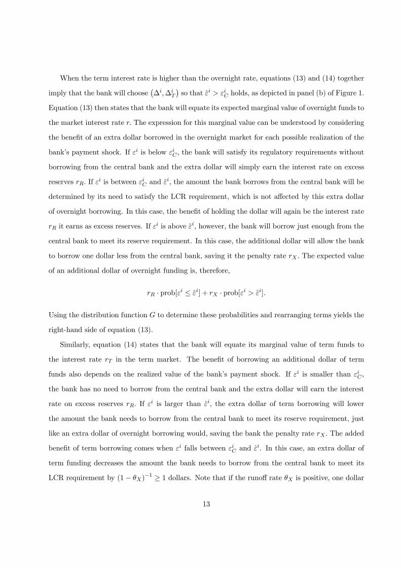
Figure 1 depicts as a function of the realized payment shock together with a density function
for this shock. The figure is drawn assuming the runoff rates in the denominator of the LCR
satisfy ; the reverse case is presented in Figure 5 in Appendix B. The blue line in each
panel represents equation (4), borrowing needed to satisfy the reserve requirement. The critical
value of the payment shock above which this component of borrowing is positive is
≡ +∆ +∆ − (8)
(a) (b)
1Slope = 11
D
X
Slope = 1
( )g
iiC
iK
iX
1Slope = 11
D
X
Slope = 1
( )g
iiC
iK
iX
ˆi
Figure 1: Bank ’s borrowing from the central bank lending facility (with )
9

The green line represents equation (6), borrowing needed to satisfy the LCR requirement. The
critical value for this case is
≡ + +∆
1− (9)
The bank’s borrowing is the upper envelope of these two lines. Note that the critical values¡
¢are determined, in part, by the bank’s trading behavior
¡∆∆
¢
As the figure shows, two distinct cases arise. In panel (a), the values¡∆∆
¢are such that
holds. In this case, the amount borrowed from the central bank’s lending facility is always
determined by the bank’s need to meet its reserve requirement; the LCR requirement is never a
binding concern. To see this, note that if is greater than , the bank will have a deficiency in
its reserve requirement and will borrow just enough from the central bank to correct this deficiency.
The figure shows that this borrowing will always be sufficient to ensure that the bank also satisfies
its LCR requirement, even when the shock is greater than
The relationship is different in panel (b) of the figure, where the values¡∆∆
¢are such that
holds. In this case, the amount borrowed from the central bank can be determined by
either of the two requirements, depending on the realized value of In particular, the amount
borrowed is determined by the LCR requirement for values of in the interval [ ] where
≡ + (1− )¡ −∆
¢+
¡ +∆
¢ −
(10)
and by the reserve requirement when is greater than
3.5 Profits
The bank earns the interest rates and on its loans and bonds, respectively. It pays an
interest rate on customer deposits and pays (or earns) and on its interbank borrowing (or
lending) in each market. The bank earns on balances held at the central bank to meet its reserve
requirement and on any excess balances. In addition, the bank faces a penalty rate
(including the value of any associated stigma effects)8 for funds borrowed from the central bank’s
8See Ennis and Weinberg (2012) and Armantier et al. (2011) for studies of the potential for stigma to be associated
with borrowing from the central bank.
10
lending facility. Bank ’s realized profit for the period can, therefore, be written as
() = +
− ¡ −
¢− ∆ − ∆ +
+max© +∆ +∆
+ − − 0ª−
Using (7) and £¤= 0 and rearranging terms, we can write the expected value of bank ’s profit
before its payment shock is realized as
[] = +
− +
− ∆ − ∆ +
¡ +∆ +∆
−¢
(11)
−( − )
∙max
½ + − −∆ −∆
(1− )
− − −∆
1− 0
¾¸
3.6 Discussion
Our model represents a minimal departure from the standard framework that can address issues
related to the LCR and its effect on both overnight and term interest rates. By studying a one-
period setting, we are necessarily abstracting from the factors that usually generate term premia,
including changes in future overnight interest rates, additional liquidity and credit risk, etc. This
approach allows us to focus directly on the effects of the liquidity regulation itself. Because the only
difference between overnight and term loans in our model is their treatment in the LCR calculation,
any term premium that arises in equilibrium is necessarily a result of the regulation.
At the same time, our model is sufficiently general to represent various types of operating
frameworks used in practice to implement monetary policy. A standard corridor framework, for
example, corresponds to situation where the central bank sets the interest rate at its lending
facility above its target rate and the interest rate paid on excess reserves below the target. The
floor system of monetary policy implementation, in contrast, involves setting equal to the target
rate.9 The model could also represent an operational framework with no reserve requirement by
setting to zero, in which case condition (3) simply requires that a bank not end the day with
an overdraft in its reserve account. For operating frameworks that allow reserve averaging, this
model can be thought of as representing either the final day of a reserve maintenance period or the
9See Goodfriend (2002) and Keister, Martin, and McAndrews (2008) for discussions of the floor system of monetary
policy implementation.
11

average values over the entire period.10
4 Equilibrium
In this section, we derive each bank’s demand for funds in the two interbank markets, aggregate
these demands across banks, and derive the equilibrium interest rates. We focus on the case where
; the corresponding analysis for the reverse case is contained in Appendix B.
4.1 The demand for interbank loans
Bank will choose its interbank borrowing activity¡∆∆
¢to maximize its expected profit (11).
Dropping terms that do not depend on the bank’s choices of ∆ and ∆ , the maximization problem
can be written as
max(∆∆
)−∆ − ∆
+
¡ +∆ +∆
−¢
(12)
−( − )
⎧⎪⎨⎪⎩ I(
)
R
³(1−)−−−∆
1−´¡¢
+R∞max{
}¡ + − −∆ −∆
¢¡¢
⎫⎪⎬⎪⎭
where the indicator function I takes the value one if the expression in parentheses is true and zero
otherwise. The solution to this problem is characterized in the following proposition, a proof of
which is provided in Appendix A.
Proposition 1 Suppose If bank will choose¡∆∆
¢so that the critical values¡
¢
defined in (8) — (10) satisfy
= + ( − )¡1−
£¤¢
and (13)
= + − 1−
¡£¤−
£¤¢ (14)
If = the bank will choose¡∆∆
¢so that these values satisfy
≥ and = + ( − )¡1−
£¤¢ (15)
10The type of framework studied here can be extended to include reserve averaging as shown by Clouse and Dow
(1999), Bartolini, Bertola, and Prati (2002), Whitesell (2006), Ennis and Keister (2008), and others.
12
When the term interest rate is higher than the overnight rate, equations (13) and (14) together
imply that the bank will choose¡∆∆
¢so that holds, as depicted in panel (b) of Figure 1.
Equation (13) then states that the bank will equate its expected marginal value of overnight funds to
the market interest rate The expression for this marginal value can be understood by considering
the benefit of an extra dollar borrowed in the overnight market for each possible realization of the
bank’s payment shock. If is below the bank will satisfy its regulatory requirements without
borrowing from the central bank and the extra dollar will simply earn the interest rate on excess
reserves If is between and the amount the bank borrows from the central bank will be
determined by its need to satisfy the LCR requirement, which is not affected by this extra dollar
of overnight borrowing. In this case, the benefit of holding the dollar will again be the interest rate
it earns as excess reserves. If is above , however, the bank will borrow just enough from the
central bank to meet its reserve requirement. In this case, the additional dollar will allow the bank
to borrow one dollar less from the central bank, saving it the penalty rate The expected value
of an additional dollar of overnight funding is, therefore,
· prob[ ≤ ] + · prob[ ]
Using the distribution function to determine these probabilities and rearranging terms yields the
right-hand side of equation (13).
Similarly, equation (14) states that the bank will equate its marginal value of term funds to
the interest rate in the term market. The benefit of borrowing an additional dollar of term
funds also depends on the realized value of the bank’s payment shock. If is smaller than
the bank has no need to borrow from the central bank and the extra dollar will earn the interest
rate on excess reserves If is larger than the extra dollar of term borrowing will lower
the amount the bank needs to borrow from the central bank to meet its reserve requirement, just
like an extra dollar of overnight borrowing would, saving the bank the penalty rate The added
benefit of term borrowing comes when falls between and . In this case, an extra dollar of
term funding decreases the amount the bank needs to borrow from the central bank to meet its
LCR requirement by (1− )−1 ≥ 1 dollars. Note that if the runoff rate is positive, one dollar
13

of term borrowing will lower the bank’s need to borrow from the central bank by more than one
dollar in this situation. The expected value of an additional dollar of term funding thus equals the
expected value of an additional dollar of overnight funding plus an extra term
− 1−
· prob[ ≤ ]
which together yield the right-hand side of (14).
When the term and overnight interest rates are equal, the bank can increase its LCR at no cost
by borrowing at term and lending the same amount of funds out overnight. The first component of
equation (15) states that, in this case, the bank will choose¡∆∆
¢so that ≥ holds, as in
panel (a) of Figure 1, and the LCR requirement is never a binding concern. The second component
says that the bank’s marginal value of funds again equals the interest rate on excess reserves
plus the expected benefit of an extra dollar of reserves in meeting the reserve requirement. The
bank will equate this marginal value to the market interest rate . Note that many pairs¡∆∆
¢will satisfy the two conditions in equation (15) and the bank will be indifferent between any of
these actions.
4.2 Aggregation
An immediate implication of Proposition 1 is that all banks will choose their interbank activity¡∆∆
¢to generate the same critical values
¡
¢ Bank ’s actual trading activity will
depend on the specifics of its initial balance sheet (2) but, once this activity has taken place,
each bank will face the same probability of a deficiency in its reserve requirement and in its LCR
requirement. In what follows, therefore, we drop the superscript from these critical values and
simply write ( ) Given the critical values determined by the proposition, bank ’s optimal
trading behavior is
∆ = + + − (1− ) and
∆ = − − + (1− )
The total demand for borrowing in the overnight interbank market can be determined by inte-
14
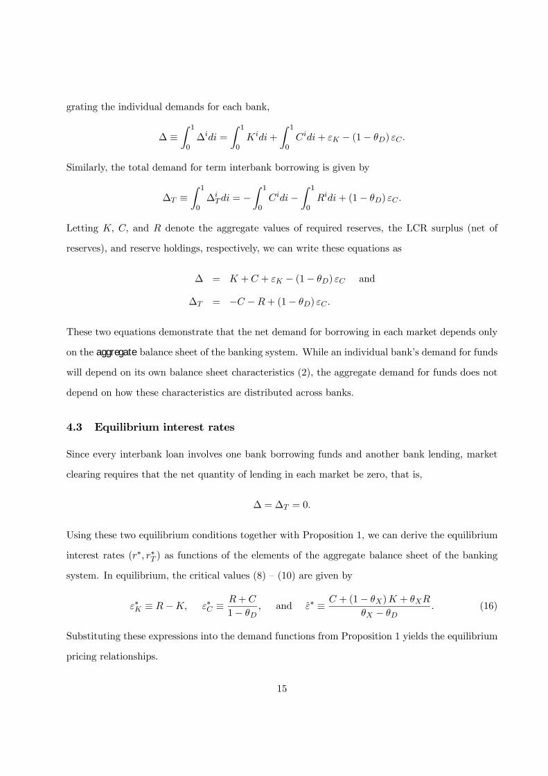
grating the individual demands for each bank,
∆ ≡Z 1
0∆ =
Z 1
0+
Z 1
0+ − (1− )
Similarly, the total demand for term interbank borrowing is given by
∆ ≡Z 1
0∆ = −
Z 1
0−
Z 1
0+ (1− )
Letting and denote the aggregate values of required reserves, the LCR surplus (net of
reserves), and reserve holdings, respectively, we can write these equations as
∆ = + + − (1− ) and
∆ = − −+ (1− )
These two equations demonstrate that the net demand for borrowing in each market depends only
on the aggregate balance sheet of the banking system. While an individual bank’s demand for funds
will depend on its own balance sheet characteristics (2), the aggregate demand for funds does not
depend on how these characteristics are distributed across banks.
4.3 Equilibrium interest rates
Since every interbank loan involves one bank borrowing funds and another bank lending, market
clearing requires that the net quantity of lending in each market be zero, that is,
∆ = ∆ = 0
Using these two equilibrium conditions together with Proposition 1, we can derive the equilibrium
interest rates (∗ ∗ ) as functions of the elements of the aggregate balance sheet of the banking
system. In equilibrium, the critical values (8) — (10) are given by
∗ ≡ − ∗ ≡+
1− and ∗ ≡ + (1− ) +
− (16)
Substituting these expressions into the demand functions from Proposition 1 yields the equilibrium
pricing relationships.
15
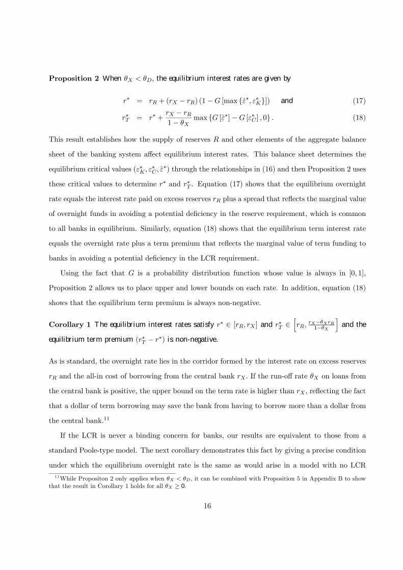
Proposition 2 When the equilibrium interest rates are given by
∗ = + ( − ) (1− [max {∗ ∗}]) and (17)
∗ = ∗ + − 1−
max { [∗]− [∗ ] 0} (18)
This result establishes how the supply of reserves and other elements of the aggregate balance
sheet of the banking system affect equilibrium interest rates. This balance sheet determines the
equilibrium critical values (∗ ∗
∗) through the relationships in (16) and then Proposition 2 uses
these critical values to determine ∗ and ∗ . Equation (17) shows that the equilibrium overnight
rate equals the interest rate paid on excess reserves plus a spread that reflects the marginal value
of overnight funds in avoiding a potential deficiency in the reserve requirement, which is common
to all banks in equilibrium. Similarly, equation (18) shows that the equilibrium term interest rate
equals the overnight rate plus a term premium that reflects the marginal value of term funding to
banks in avoiding a potential deficiency in the LCR requirement.
Using the fact that is a probability distribution function whose value is always in [0 1],
Proposition 2 allows us to place upper and lower bounds on each rate. In addition, equation (18)
shows that the equilibrium term premium is always non-negative.
Corollary 1 The equilibrium interest rates satisfy ∗ ∈ [ ] and ∗ ∈h
−1−
iand the
equilibrium term premium (∗ − ∗) is non-negative.
As is standard, the overnight rate lies in the corridor formed by the interest rate on excess reserves
and the all-in cost of borrowing from the central bank If the run-off rate on loans from
the central bank is positive, the upper bound on the term rate is higher than reflecting the fact
that a dollar of term borrowing may save the bank from having to borrow more than a dollar from
the central bank.11
If the LCR is never a binding concern for banks, our results are equivalent to those from a
standard Poole-type model. The next corollary demonstrates this fact by giving a precise condition
under which the equilibrium overnight rate is the same as would arise in a model with no LCR
11While Propositon 2 only applies when it can be combined with Proposition 5 in Appendix B to showthat the result in Corollary 1 holds for all ≥ 0
16

requirement, which we denote (the “Poole interest rate”). The corollary also shows that, under
this condition, the term premium is zero in equilibrium.
Corollary 2 (Poole, 1968) Suppose If + (1− ) + ≥ 0 the interest rate in
the overnight interbank market is given by
∗ = + ( − )(1−[∗ ]) ≡
and the term premium is zero, that is, ∗ = ∗.
Recall that ≡ − is the liquidity surplus of the banking system, net of reserves, for
LCR purposes. When this surplus is sufficiently large, adding an LCR requirement has no effect
on equilibrium interest rates. When the surplus is smaller than the bound given in Corollary 2,
however, the LCR does impact equilibrium rates. The next corollary documents the direction of
these changes: the introduction of an LCR requirement pushes the overnight rate lower and the
term rate higher.
Corollary 3 Suppose If +(1− )+ 0, the equilibrium interest rates satisfy
∗ and ∗ which implies that the term premium is strictly positive.
It bears emphasizing that the source of this term premium is purely regulatory, as our model
abstracts from the additional risks normally associated with term lending. The premium here
simply reflects the ability of term funding to raise the value of a bank’s LCR and thus help it meet
its regulatory requirements.12
5 Open market operations
We now turn our attention to the impact of open market operations on equilibrium interest rates.
In the standard model with no LCR requirement, the equilibrium overnight rate depends on bank
balance sheets only through the total quantity of reserves The same is true in our model when the
12Bonner and Eijffinger (2012) provide evidence that the introduction of a quantitative liquidity requirement in
Holland raised the average term premium on unsecured interbank loans with maturities longer than 30 days. Schmitz
(2012) also argues that the LCR requirement is likely to increase term premia.
17
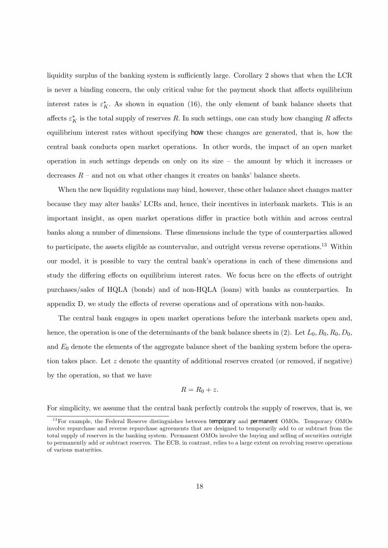
liquidity surplus of the banking system is sufficiently large. Corollary 2 shows that when the LCR
is never a binding concern, the only critical value for the payment shock that affects equilibrium
interest rates is ∗ As shown in equation (16), the only element of bank balance sheets that
affects ∗ is the total supply of reserves In such settings, one can study how changing affects
equilibrium interest rates without specifying how these changes are generated, that is, how the
central bank conducts open market operations. In other words, the impact of an open market
operation in such settings depends on only on its size — the amount by which it increases or
decreases — and not on what other changes it creates on banks’ balance sheets.
When the new liquidity regulations may bind, however, these other balance sheet changes matter
because they may alter banks’ LCRs and, hence, their incentives in interbank markets. This is an
important insight, as open market operations differ in practice both within and across central
banks along a number of dimensions. These dimensions include the type of counterparties allowed
to participate, the assets eligible as countervalue, and outright versus reverse operations.13 Within
our model, it is possible to vary the central bank’s operations in each of these dimensions and
study the differing effects on equilibrium interest rates. We focus here on the effects of outright
purchases/sales of HQLA (bonds) and of non-HQLA (loans) with banks as counterparties. In
appendix D, we study the effects of reverse operations and of operations with non-banks.
The central bank engages in open market operations before the interbank markets open and,
hence, the operation is one of the determinants of the bank balance sheets in (2). Let 0 0 00,
and 0 denote the elements of the aggregate balance sheet of the banking system before the opera-
tion takes place. Let denote the quantity of additional reserves created (or removed, if negative)
by the operation, so that we have
= 0 +
For simplicity, we assume that the central bank perfectly controls the supply of reserves, that is, we
13For example, the Federal Reserve distinguishes between temporary and permanent OMOs. Temporary OMOs
involve repurchase and reverse repurchase agreements that are designed to temporarily add to or subtract from the
total supply of reserves in the banking system. Permanent OMOs involve the buying and selling of securities outright
to permanently add or subtract reserves. The ECB, in contrast, relies to a large extent on revolving reserve operations
of various maturities.
18
abstract from uncertainty about changes in so-called autonomous factors affecting reserves.14 For
each type of operation, we first ask how it affects bank balance sheets, with a particular focus on
the resulting LCR of the banking system. We then analyze how the equilibrium interbank interest
rates ∗ and ∗ vary with the size of the operation
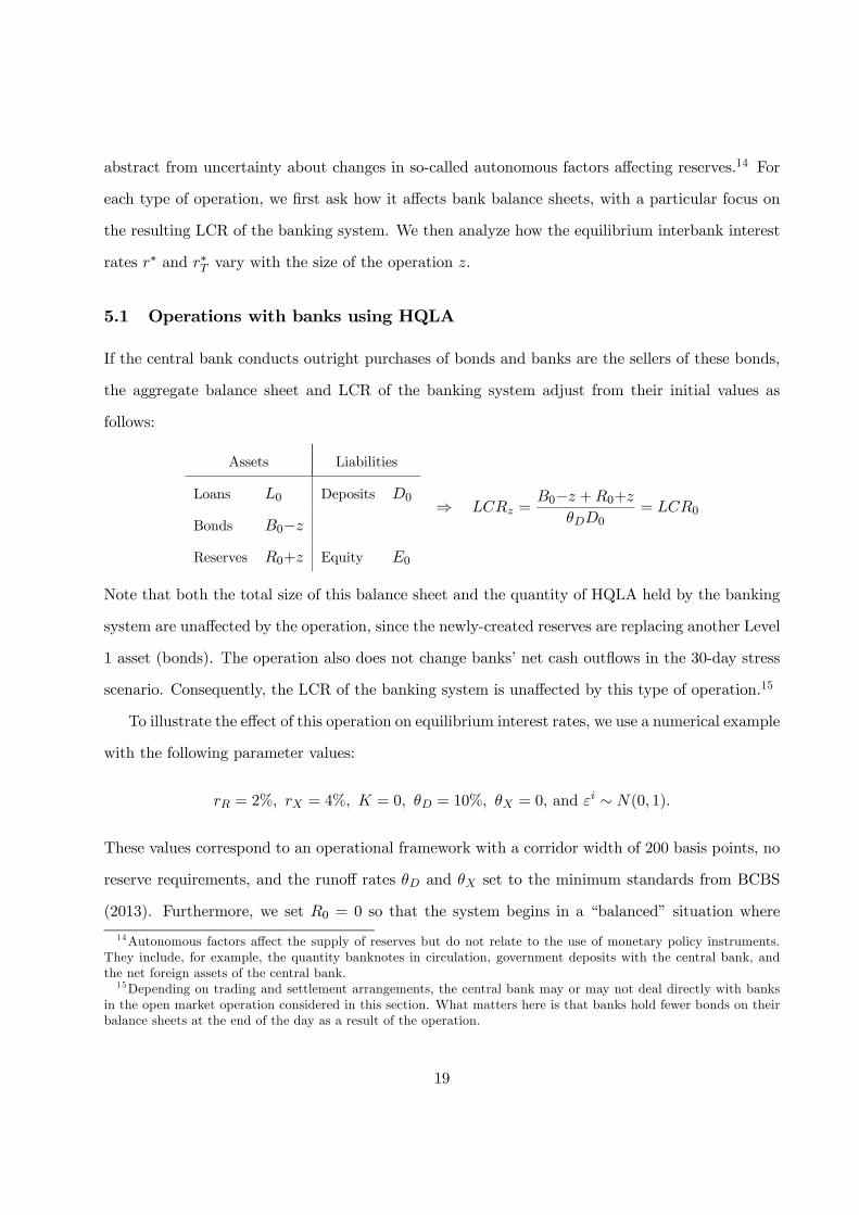
5.1 Operations with banks using HQLA
If the central bank conducts outright purchases of bonds and banks are the sellers of these bonds,
the aggregate balance sheet and LCR of the banking system adjust from their initial values as
follows:
Assets Liabilities
Loans 0 Deposits 0
Bonds 0−Reserves 0+ Equity 0
⇒ =0− +0+
0= 0
Note that both the total size of this balance sheet and the quantity of HQLA held by the banking
system are unaffected by the operation, since the newly-created reserves are replacing another Level
1 asset (bonds). The operation also does not change banks’ net cash outflows in the 30-day stress
scenario. Consequently, the LCR of the banking system is unaffected by this type of operation.15
To illustrate the effect of this operation on equilibrium interest rates, we use a numerical example
with the following parameter values:
= 2% = 4% = 0 = 10% = 0, and ∼ (0 1)
These values correspond to an operational framework with a corridor width of 200 basis points, no
reserve requirements, and the runoff rates and set to the minimum standards from BCBS
(2013). Furthermore, we set 0 = 0 so that the system begins in a “balanced” situation where
14Autonomous factors affect the supply of reserves but do not relate to the use of monetary policy instruments.
They include, for example, the quantity banknotes in circulation, government deposits with the central bank, and
the net foreign assets of the central bank.15Depending on trading and settlement arrangements, the central bank may or may not deal directly with banks
in the open market operation considered in this section. What matters here is that banks hold fewer bonds on their
balance sheets at the end of the day as a result of the operation.
19

the supply of reserves is equal to total required reserves. The equilibrium critical values for the
payment shock in (16) then reduce to
∗ = ∗ =009
and ∗ = − 001
where 0 ≡ 0 + 0 is the liquidity surplus of the banking system prior to the operation.
Figure 2 depicts equilibrium interest rates as functions of the change in reserves . When banks
have a large liquidity surplus, as in panel (a), the LCR is never a binding concern. In this case, the
result in Corollary 2 applies for all values of in the figure: the effects of open market operations
are the same as in the standard model and there is no term premium. Note that the overnight
interest rate is at the midpoint of the corridor when there are zero excess reserves in the banking
system ( = 0); this point has been emphasized by Woodford (2001), Whitesell (2006) and others.
(a) 0 = 2 (b) 0 = 1
-2 -1 0 1 2
2
3
4
5
z
pct.
-2 -1 0 1 2
2
3
4
5
z
pct.
(c) 0 = 0 (d) 0 = −1
-2 -1 0 1 2
2
3
4
5
z
pct.
-2 -1 0 1 2
2
3
4
5
z
pct.
– overnight rate (∗), - - term rate (∗ ).
Figure 2: Effect of open market operations with banks using HQLA
20
When the liquidity surplus is smaller, as in panel (b), the figure shows how increasing the supply
of reserves can introduce the effects described in Corollary 3. In particular, for sufficiently large
values of the overnight rate is pushed lower — rapidly approaching the floor of the corridor —
and a term premium emerges. The bottom two panels show that as the liquidity position of the
banking system deteriorates further, these effects arise for smaller values of and the size of the
term premium increases. In panel (d), a substantial quantity of reserves must be removed to lift
the overnight rate off the floor of the corridor, while the term rate remains close to the ceiling of
the corridor regardless of the size of the operation.
To understand these patterns, recall that adding reserves through this type of operation does not
change the total stock of HQLA held by the banking system, but shifts its composition to include
more reserves. The likelihood that a bank will face an LCR deficiency is, therefore, unaffected
by the operation, while the likelihood of it facing a reserve deficiency decreases. Looking back at
Figure 1, higher values of tend to move banks away from the situation depicted in panel (a)
and toward the situation depicted in panel (b). Once panel (b) applies, additional increases in
the supply of reserves sharply reduce the overnight rate as the reserve requirement becomes less
likely to be a binding concern. Such increases have no effect on the term rate, however, since term
borrowing helps a bank meet both types of requirement.
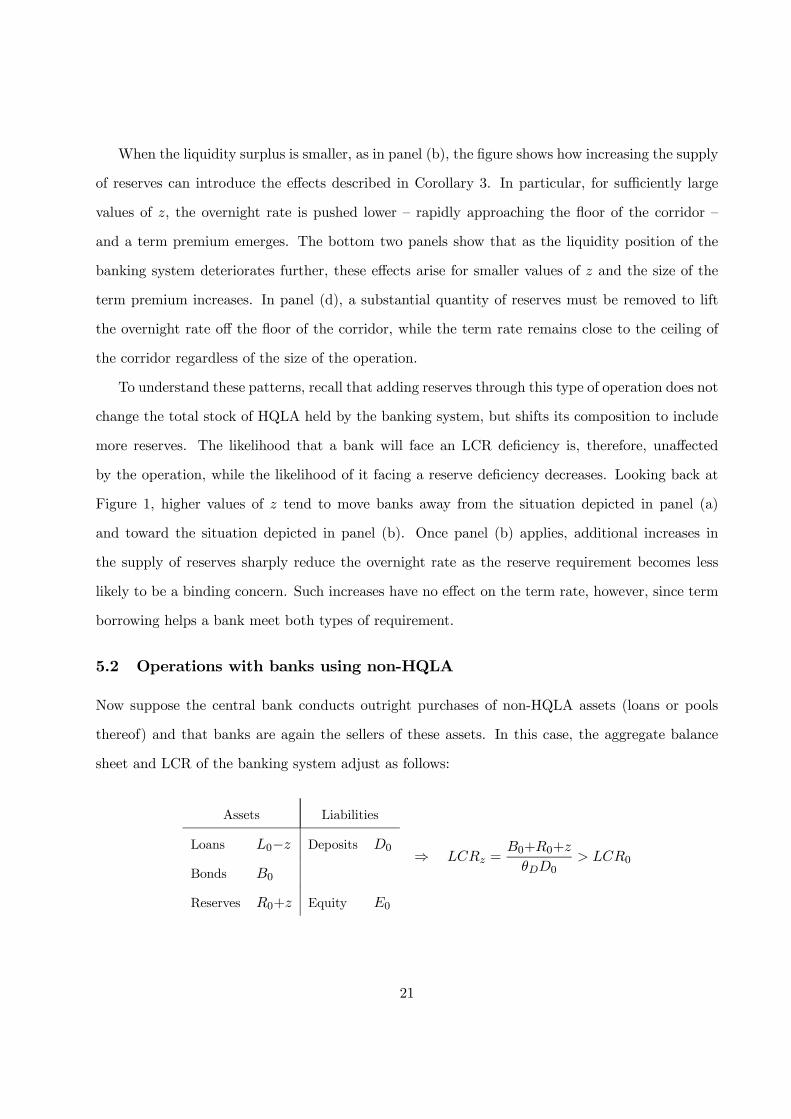
5.2 Operations with banks using non-HQLA
Now suppose the central bank conducts outright purchases of non-HQLA assets (loans or pools
thereof) and that banks are again the sellers of these assets. In this case, the aggregate balance
sheet and LCR of the banking system adjust as follows:
Assets Liabilities
Loans 0− Deposits 0
Bonds 0
Reserves 0+ Equity 0
⇒ =0+0+
0 0
21
While the size of this balance sheet is again unchanged, the operation now substitutes reserves for
loans on bank balance sheets and thereby increases the pool of HQLA. There is again no effect
on net cash outflows and, hence, the operation raises the LCR of the banking system. Adding
reserves through purchases of non-HQLA thus makes the LCR less likely to bind and, as a result,
the demand for interbank borrowing is more likely to be determined by the reserve requirement,
which tends to lower the term premium. In the central bank instead sells loans using this type of
operation, the LCR of the banking system will decrease and the value of term funding will tend to
rise more than the value of overnight funding.
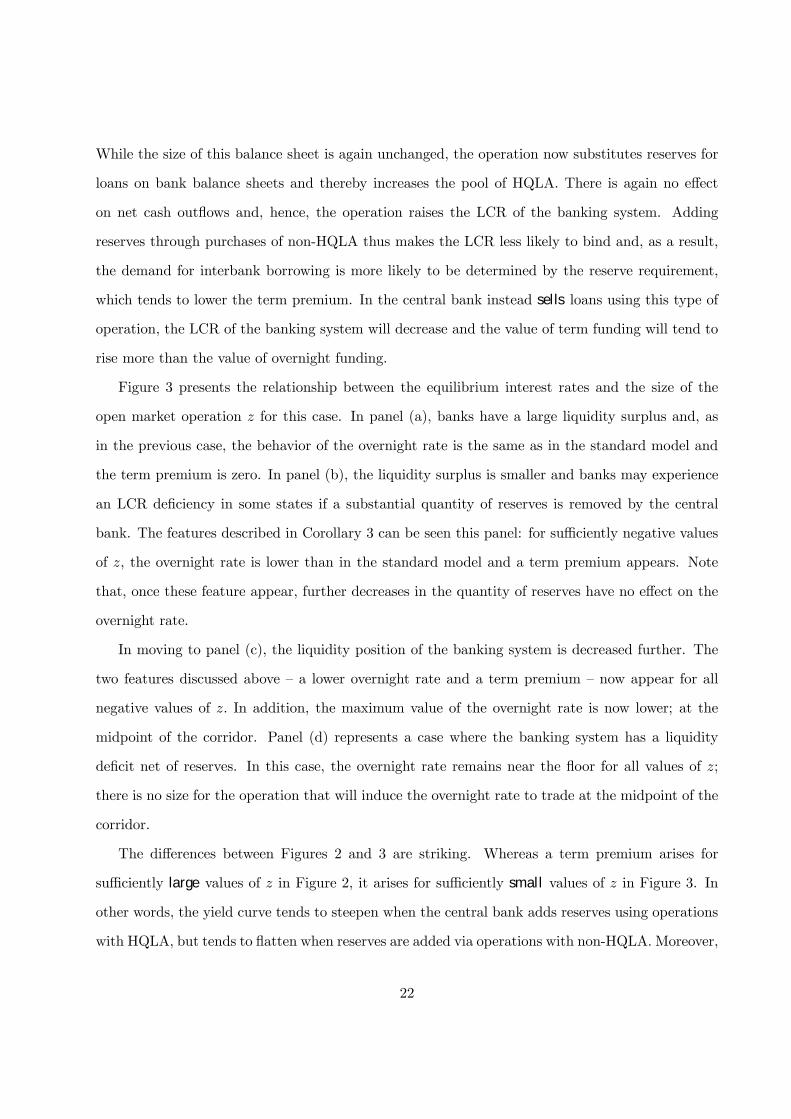
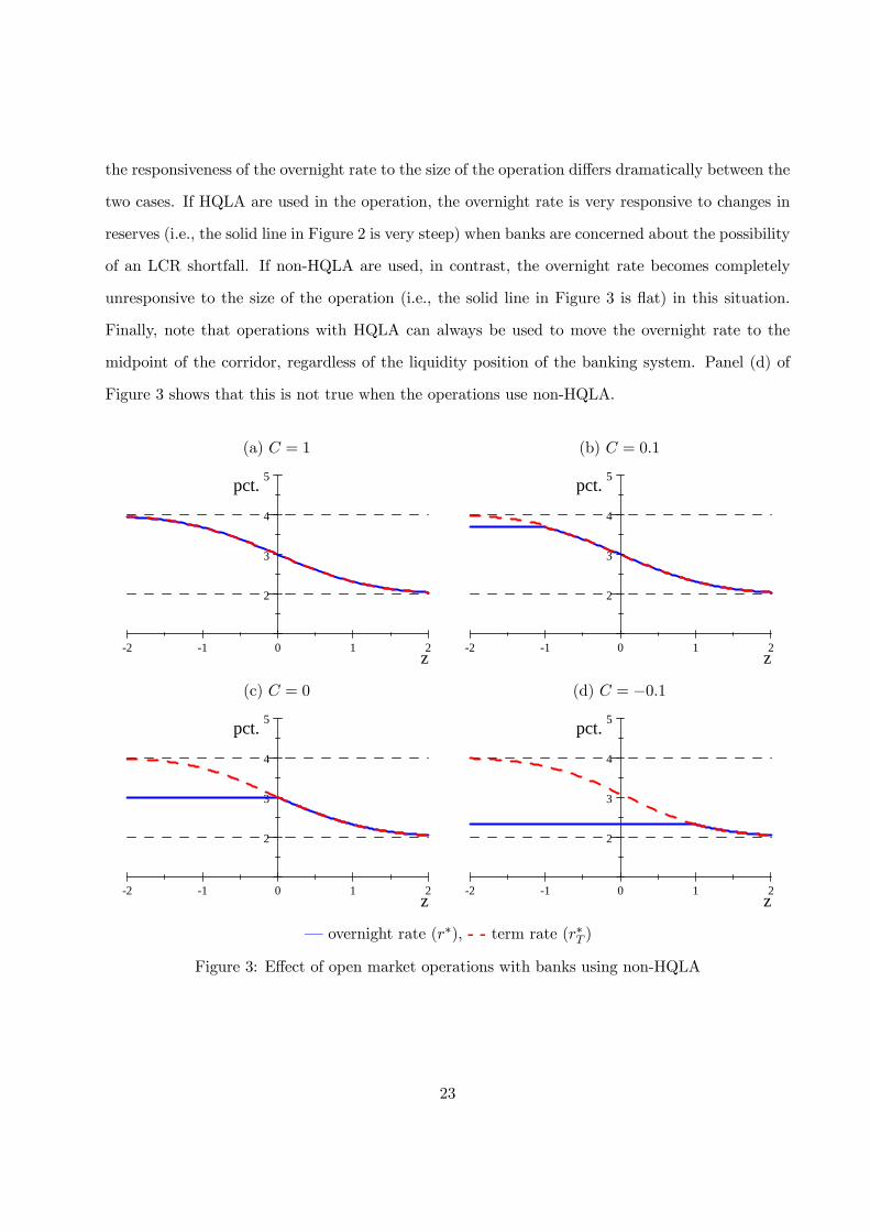
Figure 3 presents the relationship between the equilibrium interest rates and the size of the
open market operation for this case. In panel (a), banks have a large liquidity surplus and, as
in the previous case, the behavior of the overnight rate is the same as in the standard model and
the term premium is zero. In panel (b), the liquidity surplus is smaller and banks may experience
an LCR deficiency in some states if a substantial quantity of reserves is removed by the central
bank. The features described in Corollary 3 can be seen this panel: for sufficiently negative values
of , the overnight rate is lower than in the standard model and a term premium appears. Note
that, once these feature appear, further decreases in the quantity of reserves have no effect on the
overnight rate.
In moving to panel (c), the liquidity position of the banking system is decreased further. The
two features discussed above — a lower overnight rate and a term premium — now appear for all
negative values of In addition, the maximum value of the overnight rate is now lower; at the
midpoint of the corridor. Panel (d) represents a case where the banking system has a liquidity
deficit net of reserves. In this case, the overnight rate remains near the floor for all values of ;
there is no size for the operation that will induce the overnight rate to trade at the midpoint of the
corridor.
The differences between Figures 2 and 3 are striking. Whereas a term premium arises for
sufficiently large values of in Figure 2, it arises for sufficiently small values of in Figure 3. In
other words, the yield curve tends to steepen when the central bank adds reserves using operations
with HQLA, but tends to flatten when reserves are added via operations with non-HQLA. Moreover,
22
the responsiveness of the overnight rate to the size of the operation differs dramatically between the
two cases. If HQLA are used in the operation, the overnight rate is very responsive to changes in
reserves (i.e., the solid line in Figure 2 is very steep) when banks are concerned about the possibility
of an LCR shortfall. If non-HQLA are used, in contrast, the overnight rate becomes completely
unresponsive to the size of the operation (i.e., the solid line in Figure 3 is flat) in this situation.
Finally, note that operations with HQLA can always be used to move the overnight rate to the
midpoint of the corridor, regardless of the liquidity position of the banking system. Panel (d) of
Figure 3 shows that this is not true when the operations use non-HQLA.
(a) = 1 (b) = 01
-2 -1 0 1 2
2
3
4
5
z
pct.
-2 -1 0 1 2
2
3
4
5
z
pct.
(c) = 0 (d) = −01
-2 -1 0 1 2
2
3
4
5
z
pct.
-2 -1 0 1 2
2
3
4
5
z
pct.
– overnight rate (∗), - - term rate (∗ )
Figure 3: Effect of open market operations with banks using non-HQLA
23
These results illustrate how the effects of an open market operation can depend critically on
its structure in the presence of an LCR requirement. In the next section, we investigate how the
magnitude of these effects depends on one of the parameters of the regulation: the runoff-rate
assigned to secured loans from the central bank.
6 Changing the runoff rate
The original LCR rules (BCBS, 2010) included a review clause that allowed for changes to be
made to address concerns about possible unintended consequences. In January 2013, the Basel
Committee issued a revised version of the rules text (BCBS, 2013). This revision included several
changes to the LCR requirement, including an expansion in the range of assets eligible as HQLA
and refinements to minimum standards for various inflow and outflow rates to better reflect actual
experience in times of stress. Of particular interest in our context is the decision to reduce minimum
the outflow rate on maturing secured funding transactions with central banks — our parameter
— from 25% to 0%. How does changing this parameter affect the impact of the LCR on the process
of monetary policy implementation?
The following proposition shows that decreasing tends to mitigate the effects of the LCR
on equilibrium interest rates in our model. In particular, lowering will tend to increase the
overnight rate and decrease the term rate, pulling both rates closer to the interest rate that
prevails when there is no LCR requirement.
Proposition 3 The equilibrium overnight rate ∗ is weakly decreasing in and the equilibrium
term rate ∗ is weakly increasing in .
This result applies for all ≥ 0 including both the case of studied in Section 5 and the
case of studied in Appendix B. A proof of this proposition is presented in Appendix C.
Figure 4 illustrates this result by plotting the equilibrium interest rates (∗ ∗ ) associated with
two different values of in each panel: = 025 and = 0 These runoff rates correspond
to the minimum standards under the original and revised LCR rules, respectively. The two panels
of the figure corresponds to the case where the central bank conducts outright purchases/sales of
24

HQLA (panel a) and of non-HQLA (panel b). The initial value of the liquidity surplus of the
banking system (net of reserves) is set to 0 = 0 which means that the interest rates associated
with = 0 are the same those in panel (c) of Figure 2 (for HQLA) and Figure 3 (for non-HQLA).
The new curves in each panel are the equilibrium interest rates associated with = 025
For the case of operations with HQLA, when is sufficiently small, the LCR is not a binding
concern and the overnight rate is the same as in the standard model regardless of the value of
For sufficiently large values of the overnight rate is at the floor of the corridor for both values of
For intermediate values of however, we see that the overnight rate is lower when = 025
The difference can be significant: when = 0 the overnight rate is at the midpoint of the corridor
with = 0 but at the floor of the corridor with the higher value of Similarly, the two dashed
lines show that the term rate tends to be higher when = 025 Overall, panel (a) of Figure 4
shows how moving from the higher value of the runoff rate to = 0 pushes the overnight and
term rates closer together, although a substantial term premium remains when is positive.
(a) HQLA (b) Non-HQLA
0 = 0
-2 -1 0 1 2
2
4
z
pct.
-2 -1 0 1 2
2
4
z
pct.
= 25%: – ∗, - - ∗ , = 25%: – ∗, - - ∗ , = 0%: – ∗, - - ∗ . = 0%: – ∗, - - ∗ .
Figure 4: Comparing = 0 and for open market operations with banks
Panel (b) presents the corresponding figure for the case where the central bank conducts outright
purchases/sales of non-HQLA. The same patterns arise here, and the differences between the two
cases are even larger. With = 0 the overnight rate lies at the midpoint of the corridor for all
25
0 With = 025 in contrast, the overnight rate lies on the floor of the corridor for all 0
and is lower than the interest rate from the standard model for any value of In addition, the term
interest rate rises above the penalty rate when = 025 since a dollar of term borrowing in
this case will save the bank from having to borrow (1− )−1 1 dollars from the central bank’s
lending facility in some states.
While the figure illustrates how lowering mitigates the effects of the LCR on equilibrium
interest rates, note that these effects remain large even for the lowest possible value of the para-
meter, = 0 Thus, when banks face the possibility of an LCR shortfall, the introduction of an
LCR requirement can have a significant impact on the process of monetary policy implementation
regardless of the value chosen for parameter
7 Conclusions
The liquidity coverage ratio (LCR) introduced as part of the Basel III regulatory framework will
change banks’ demand for liquid assets and their behaviour in money markets. As many central
banks implement monetary policy by targeting short-term interbank rates, it is important to un-
derstand the nature of these changes. What impact will the LCR requirement have on overnight
and longer-term rates? How will these changes affect a central bank’s ability to control interest
rates using open market operations? We provide a first step in answering these questions.
Our model points to four central conclusions. First, the impact of the LCR will depend on the
liquidity position of the banking system. If banks have a large surplus of liquid assets, introducing
an LCR requirement has little or no effect. When banks face the possibility of an LCR shortfall,
however, the requirement can change equilibrium interest rates substantially. Second, once the LCR
is in place, the effect of an open market operation depends on how it is structured as well as its size.
For example, outright purchases of high-quality liquid assets (HQLA) tend to affect the overnight
interest rate and steepen the short end of the yield curve, while purchases of non-HQLA may
bring little-to-no change in the overnight rate and a flattening of the yield curve. In our model, the
central bank would need to consider how an operation affects all of the components of bank balance
sheets that enter into the LCR calculation. Third, the LCR will likely introduce a regulatory-driven
26
term premium, making the short end of the yield curve steeper. Finally, the treatment of central
bank loans in the LCR calculation is an important determinant of the regulation’s effects. By
lowering the runoff rate assigned to these loans in the stress scenario, the final LCR rules described
in BCBS (2013) mitigate – but do not eliminate – the regulation’s effects on monetary policy
implementation relative to the initial proposal.
There are several steps central banks can take to counter the possible impact of the regulation
on the implementation of monetary policy. In some jurisdictions, it might be advantageous for
the central bank to target a term interest rate rather than the overnight rate. The Swiss National
Bank, for example, already implements its monetary policy in part by targeting the three-month
Swiss franc Libor rate. Another option is for the central bank to lend high-quality liquid assets to
banks in a form other than reserves. Inspiration for such facilities can be taken from the Bank of
England’s Discount Window and the Federal Reserve’s Term Securities Lending Facility, which have
allowed participants to borrow, for a fee, gilts or treasuries against a range of less-liquid collateral.
The LCR rules also permit central banks in jurisdictions where high-quality liquid assets may be
in short supply to set up a contractually-committed liquidity facility that can be counted as part
of a bank’s stock of HQLA.
We have assumed here that the central bank’s lending facility accepts illiquid assets as collateral
and, hence, that banks can use this facility to increase their unencumbered holdings of HQLA and
thereby meet their LCR requirement. If that is not the case, banks will likely shift their balance
sheets to include more HQLA on an on-going basis, a move that could potentially affect other parts
of the monetary policy transmission mechanism. At the June 2012 meeting of the Bank of England’s
Monetary Policy Committee (MPC), for example, concern was expressed “that regulatory liquidity
requirements might be increasing the demand for reserves, attenuating the impact on the economy
of the MPC’s asset purchase programme and the associated increase in the supply of reserves.”16
An interesting avenue for future research would be to use, an expanded model that accounts for
how banks arrive at their initial balance sheets to understand how the new LCR requirement may
impact these other aspects of monetary policy.17
16See page 9 of www.bankofengland.co.uk/publications/Documents/records/fpc/pdf/2012/record1207.pdf17Covas and Driscoll (2013) study how liquidity regulations can affect the composition of bank balance sheets in a
27
8 Appendices
A Proof of Proposition 1
To deal with the indicator function in the objective function (12), we examine the first-order
conditions in the regions ≥ and separately. If
≥ holds, the indicator function
is zero and we have max©
ª= . The marginal benefits of overnight and term funding in
this case are given by
[]
∆= − + + ( − )
Z ∞
¡¢ (19)
and
[]
∆
= − + + ( − )
Z ∞
¡¢ (20)
In the region where holds, the value of the indicator function is one, we havemax©
ª=
and the marginal benefits are
[]
∆= − + + ( − )
Z ∞
¡¢ (21)
and
[]
∆
= − + + ( − )
Ã1
1−
Z
¡¢ +
Z ∞
¡¢
! (22)
For the first part of the proposition, suppose that holds and consider the region where
≥ In this case, expressions (19) and (20) imply
[]
∆
[]
∆
meaning that the bank could increase its expected profit by borrowing one dollar less in the term
market and one dollar more in the overnight market. It follows that the solution to the problem
cannot lie in this region and, hence, must satisfy This solution is characterized by setting
the derivatives (21) and (22) to zero, which yields
= + ( − )¡1−
£¤¢
general equilibrium setting, but do not address issues related to monetary policy
28
and
= + ( − )
Ã1−
£¤+
£¤−
£¤
1−
!
which are equivalent to equations (13) and (14) from the statement of the proposition.
Now suppose that = holds and consider the region where holds. In this case, the
derivatives in (21) and (22) imply
[]
∆
[]
∆
meaning that the bank could increase its expected profit by borrowing one dollar more in the term
market and one dollar less in the overnight market. It follows that the solution to the problem in
this case cannot lie in this region and must instead satisfy ≥ The problem is solved in this
case by any pair¡∆∆
¢that equates both (19) and (20) to zero, which requires that satisfy
= + ( − )¡1−
£¤¢
This is equation (15) from the statement of the proposition. ¥
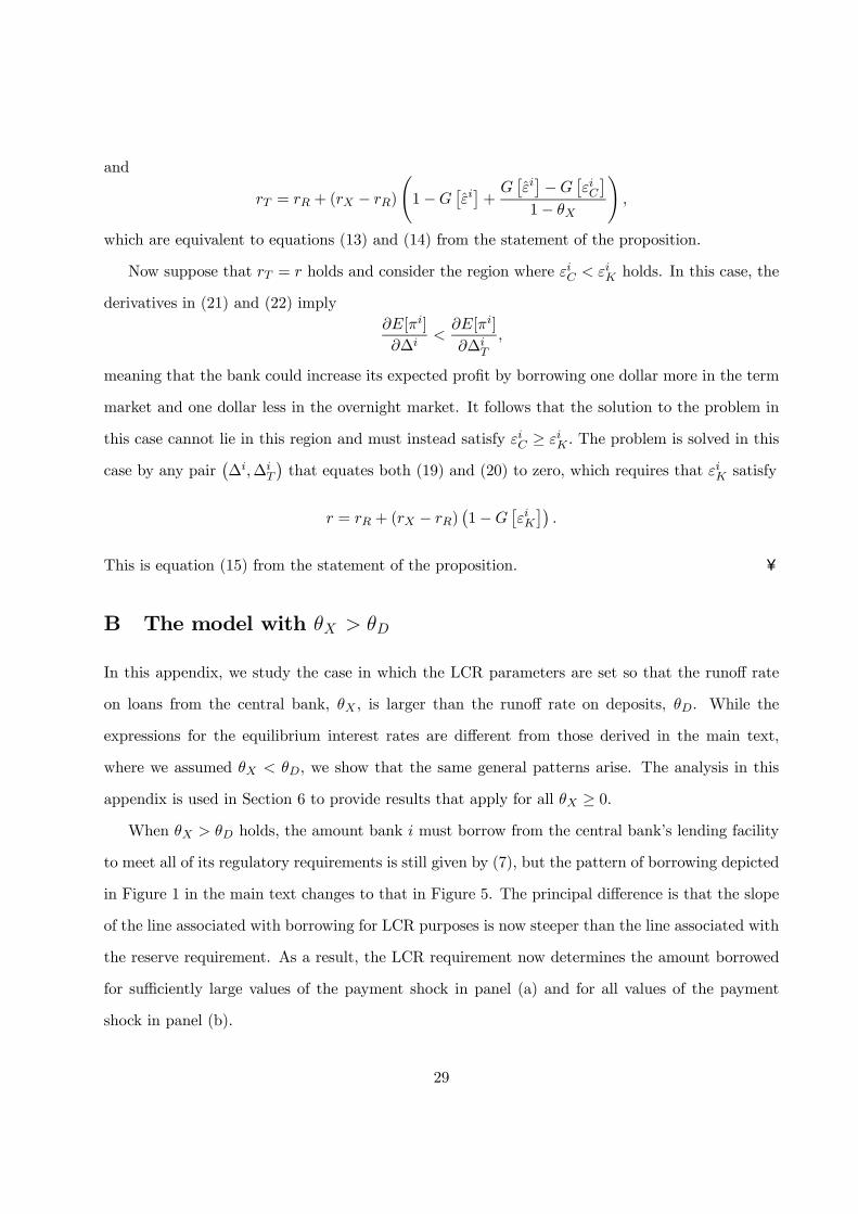
B The model with
In this appendix, we study the case in which the LCR parameters are set so that the runoff rate
on loans from the central bank, , is larger than the runoff rate on deposits, . While the
expressions for the equilibrium interest rates are different from those derived in the main text,
where we assumed , we show that the same general patterns arise. The analysis in this
appendix is used in Section 6 to provide results that apply for all ≥ 0When holds, the amount bank must borrow from the central bank’s lending facility
to meet all of its regulatory requirements is still given by (7), but the pattern of borrowing depicted
in Figure 1 in the main text changes to that in Figure 5. The principal difference is that the slope
of the line associated with borrowing for LCR purposes is now steeper than the line associated with
the reserve requirement. As a result, the LCR requirement now determines the amount borrowed
for sufficiently large values of the payment shock in panel (a) and for all values of the payment
shock in panel (b).
29
(a) (b)
1Slope = 11
D
X
Slope = 1
( )g
iiC
iK ˆi
iX 1Slope = 11
D
X
Slope = 1
( )g
iiC
iK
iX
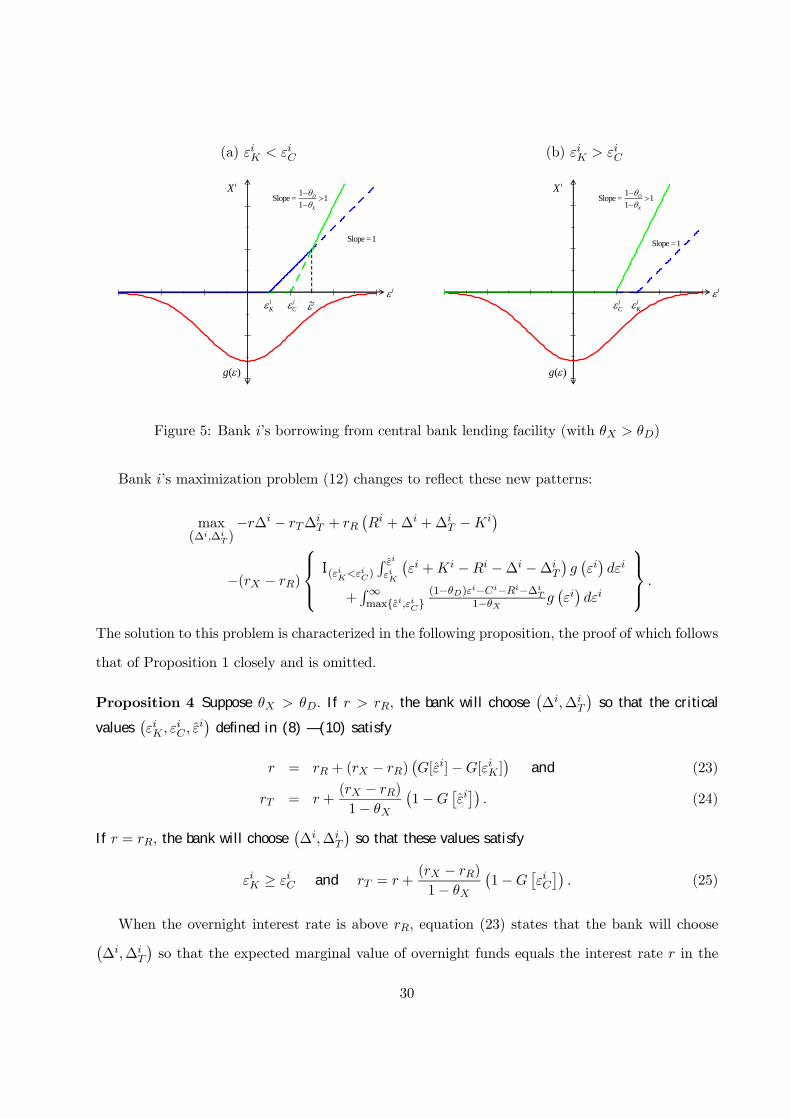
Figure 5: Bank ’s borrowing from central bank lending facility (with )
Bank ’s maximization problem (12) changes to reflect these new patterns:
max(∆∆
)−∆ − ∆
+
¡ +∆ +∆
−¢
−( − )
⎧⎪⎨⎪⎩ I(
)
R
¡ + − −∆ −∆
¢¡¢
+R∞max{
}(1−)−−−∆
1− ¡¢
⎫⎪⎬⎪⎭
The solution to this problem is characterized in the following proposition, the proof of which follows
that of Proposition 1 closely and is omitted.
Proposition 4 Suppose If the bank will choose¡∆∆
¢so that the critical
values¡
¢
defined in (8) — (10) satisfy
= + ( − )¡[]−[ ]
¢and (23)
= +( − )
1−
¡1−
£¤¢ (24)
If = the bank will choose¡∆∆
¢so that these values satisfy
≥ and = +( − )
1−
¡1−
£¤¢ (25)
When the overnight interest rate is above equation (23) states that the bank will choose¡∆∆
¢so that the expected marginal value of overnight funds equals the interest rate in the
30
overnight market. This entails choosing¡∆∆
¢so that holds, as depicted in panel
(a) of Figure 5. Similarly, equation (24) states that the bank will equate its marginal value of
term funds to the interest rate in the term market. This marginal value is equal to the value
of overnight funds plus a term premium that is proportional to the probability that will be in
the range where the bank’s borrowing from the central bank is determined by its need to meet the
LCR requirement.
When the overnight interest rate is equal to the bank can increase its reserve holdings at
no cost by borrowing funds in the overnight market and holding the funds in its reserve account.
The first component of equation (25) states that, in this case, the bank will choose¡∆∆
¢so
that ≥ holds, as in panel (b) of Figure 1, and the reserve requirement is never a binding
concern. The second component says that the bank’s marginal value of term funds again equals
the value of overnight funds plus a term premium, and that the bank will equate this marginal
value to the interest rate in the term market. Note that many pairs¡∆∆
¢will satisfy the
two conditions in equation (25) and the bank will be indifferent between any of these actions.
Substituting the equilibrium critical values from (16) into the demand functions from Proposi-
tion 4 yields the equilibrium pricing relationships.
Proposition 5 When the equilibrium interest rates are given by
∗ = + ( − )max{[∗]−[∗ ] 0} and (26)
∗ = ∗ +( − )
1− (1−[max{∗ ∗}]) (27)
This result provides the counterpart to Proposition 2 in the main text. As before, the equilibrium
overnight rate is equal to the interest rate on reserves plus a spread that reflects the marginal
value of overnight funds in avoiding a deficiency in a bank’s reserve requirement. The equilibrium
term rate equals the overnight rate plus a term premium that reflects the marginal value of term
funding in avoiding a deficiency in the LCR requirement. The expressions differ from those in
Proposition 2 because of the different pattern of borrowing needed to satisfy the bank’s two
requirements, as depicted in Figures 1 and 5. Proposition 5 is used in Section 6 of the text (especially
in establishing Proposition 3) to provide results that apply for all ≥ 0
31

C Proof of Proposition 3
First note that the equilibrium critical values ∗ and ∗ in (16) do not depend on whereas ∗
does depend on with
∗
= − + (1− ) +
( − )2 (28)
for any 6= The proof is divided into three cases.
Case () : The region where
In this case, Proposition 2 shows that ∗ is a decreasing function of
max {∗ ∗} (29)
If ∗ ≤ ∗ then (29) is independent of For the reverse case, one can use (16) and (28) to show
that the following inequalities are equivalent:
∗ ∗ ∗ ⇔ + (1− ) + 0 ⇔ ∗
0 (30)
This expression shows that if ∗ ∗ then ∗ — and hence (29) — is strictly increasing in
The expression in (29) is thus a weakly increasing function of and, therefore, ∗ is a weakly
decreasing function of in the region
Proposition 2 also shows that ∗ is a strictly increasing function of
max { [∗]− [∗ ] 0} (31)
Again using (30), it follows that (31) is a weakly increasing function of Combined with the
(1− ) term in the denominator of (18), this implies that ∗ is a weakly decreasing function of
in the region
Case () : The region where
We now establish that these same results hold in the region In this case, Proposition 5
shows that ∗ is a strictly decreasing function of
max { [∗]− [∗ ] 0} (32)
32
Equations (16) and (28) imply that, for this case, the following inequalities are equivalent:
∗ ∗ ∗ ⇔ + (1− ) + 0 ⇔ ∗
0 (33)
In other words, we have either ∗ ≤ ∗ in which case (32) is zero and independent of or
∗ ∗ in which chase ∗ and (32) are strictly decreasing functions of The expression in (32)
is thus a weakly decreasing function of which implies that ∗ is a weakly decreasing function
of in the region as well.
Similarly, Proposition 5 shows that ∗ is a decreasing function of
max {∗ ∗} (34)
Again using (33), it follows that (34) is a weakly decreasing function of Combined with the
(1− ) term in the denominator of (27), this implies that ∗ is a weakly decreasing function of
in the region
Case () : Comparing across regions
What remains is to connect the two cases above by establishing that ∗ is always lower in case ()
than in case () and that the reverse holds for ∗ For example, while there may be a discontinuity
in the function ∗ () at = the discontinuity would always represent a jump down in the
overnight rate and not a jump up.
Let (∗ ∗ ∗) denote the equilibrium values associated with some Then using Propo-
sitions 2 and 5, we can write the difference between ∗ and ∗ as
∗ − ∗ = ( − ) (1− [max {∗ ∗}]−max { [∗]− [∗ ] 0}) (35)
Using (16), one can show that the ordering of the equilibrium critical values must be either
∗ ∗ ∗ ∗ (36)
or
∗ ≤ ∗ ≤ ∗ ≤ ∗ (37)
33
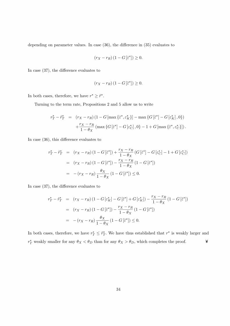
depending on parameter values. In case (36), the difference in (35) evaluates to
( − ) (1− [∗]) ≥ 0
In case (37), the difference evaluates to
( − ) (1− [∗]) ≥ 0
In both cases, therefore, we have ∗ ≥ ∗
Turning to the term rate, Propositions 2 and 5 allow us to write
∗ − ∗ = ( − ) (1− [max {∗ ∗}]−max { [∗]− [∗ ] 0})
+ − 1−
(max { [∗]− [∗ ] 0}− 1 + [max {∗ ∗}])
In case (36), this difference evaluates to
∗ − ∗ = ( − ) (1− [∗]) + − 1−
( [∗]− [∗ ]− 1 + [∗ ])
= ( − ) (1− [∗])− − 1−
(1− [∗])
= − ( − )
1− (1− [∗]) ≤ 0
In case (37), the difference evaluates to
∗ − ∗ = ( − ) (1− [∗ ]− [∗] + [∗ ])− − 1−
(1− [∗])
= ( − ) (1− [∗])− − 1−
(1− [∗])
= − ( − )
1− (1− [∗]) ≤ 0
In both cases, therefore, we have ∗ ≤ ∗ We have thus established that ∗ is weakly larger and
∗ weakly smaller for any than for any which completes the proof. ¥
34
D Other types of open market operations
In this appendix, we study the effects of two types of open market operations not considered in
Section 5: () reverse operations and () operations with non-bank counterparties, that is, with
institutions that are not active in interbank markets and not subject to reserve or LCR requirements.
D.1 Reverse operations
In a reverse operation, the exchange of reserves for collateral between the central bank and its
counterparty is reversed at a pre-specified future date. As with the outright operations studied in
Section 5, the effects of a reverse operation depend crucially on the type of assets used.
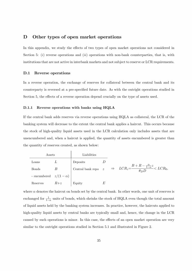
D.1.1 Reverse operations with banks using HQLA
If the central bank adds reserves via reverse operations using HQLA as collateral, the LCR of the
banking system will decrease to the extent the central bank applies a haircut. This occurs because
the stock of high-quality liquid assets used in the LCR calculation only includes assets that are
unencumbered and, when a haircut is applied, the quantity of assets encumbered is greater than
the quantity of reserves created, as shown below:
Assets Liabilities
Loans Deposits
Bonds Central bank repo
- encumbered (1− )
Reserves + Equity
⇒ = +−
1−
0
where denotes the haircut on bonds set by the central bank. In other words, one unit of reserves is
exchanged for 11− units of bonds, which shrinks the stock of HQLA even though the total amount
of liquid assets held by the banking system increases. In practice, however, the haircuts applied to
high-quality liquid assets by central banks are typically small and, hence, the change in the LCR
caused by such operations is minor. In this case, the effects of an open market operation are very
similar to the outright operations studied in Section 5.1 and illustrated in Figure 2.
35
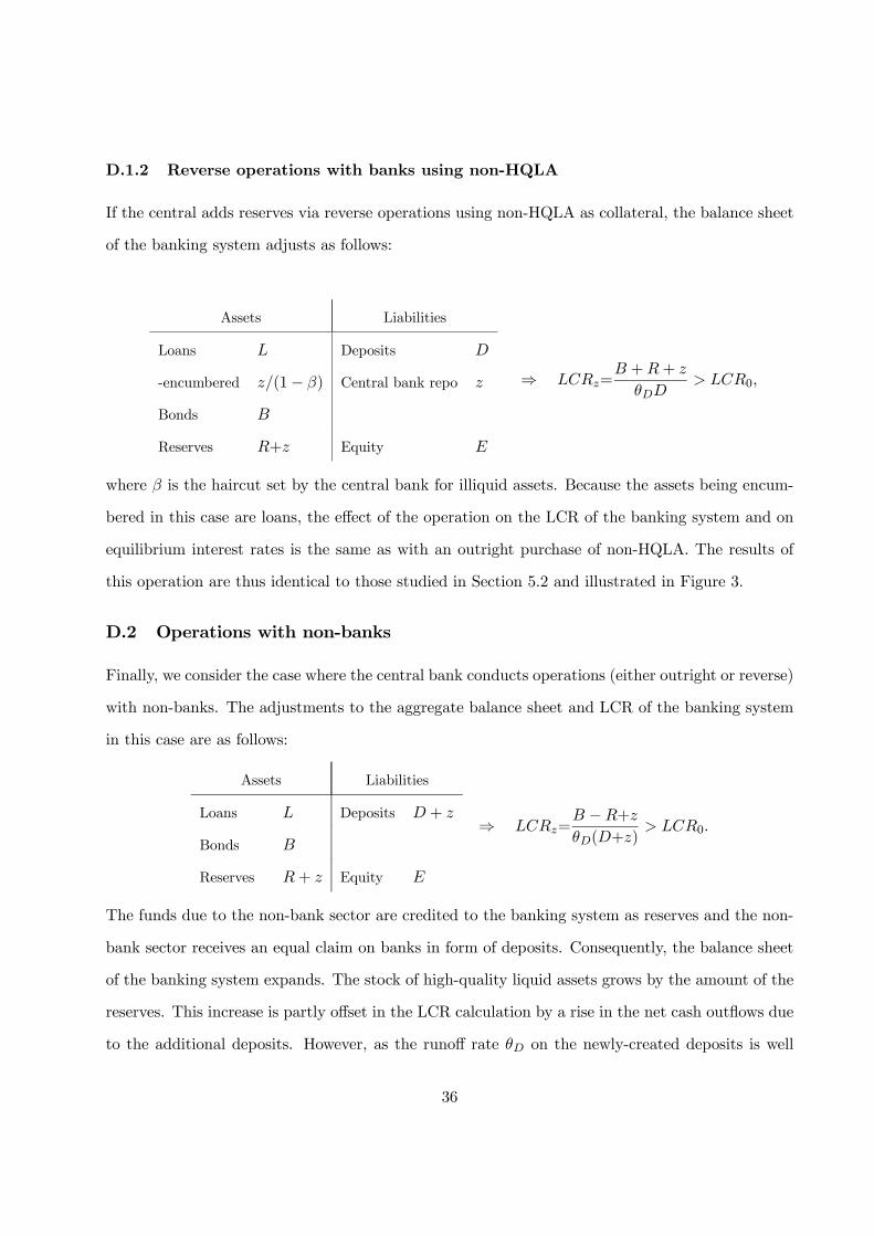
D.1.2 Reverse operations with banks using non-HQLA
If the central adds reserves via reverse operations using non-HQLA as collateral, the balance sheet
of the banking system adjusts as follows:
Assets Liabilities
Loans Deposits
-encumbered (1− ) Central bank repo
Bonds
Reserves + Equity
⇒ = ++
0
where is the haircut set by the central bank for illiquid assets. Because the assets being encum-
bered in this case are loans, the effect of the operation on the LCR of the banking system and on
equilibrium interest rates is the same as with an outright purchase of non-HQLA. The results of
this operation are thus identical to those studied in Section 5.2 and illustrated in Figure 3.
D.2 Operations with non-banks
Finally, we consider the case where the central bank conducts operations (either outright or reverse)
with non-banks. The adjustments to the aggregate balance sheet and LCR of the banking system
in this case are as follows:
Assets Liabilities
Loans Deposits +
Bonds
Reserves + Equity
⇒ = −+
(+) 0
The funds due to the non-bank sector are credited to the banking system as reserves and the non-
bank sector receives an equal claim on banks in form of deposits. Consequently, the balance sheet
of the banking system expands. The stock of high-quality liquid assets grows by the amount of the
reserves. This increase is partly offset in the LCR calculation by a rise in the net cash outflows due
to the additional deposits. However, as the runoff rate on the newly-created deposits is well
36

below 100%, the LCR rises. Notice that, in this case, the type of assets involved does not matter
for determining the change in the LCR.
Figure 6 illustrates the effects of open market operations with non-banks. As in the case of
operations with banks using non-HQLA (Figure 3), a term premium tends to arise when is small.
The size of the term premium is no longer monotone in however. As shown in panels (b) and
(c), the term premium may be largest for values of slightly below zero and then shrink as reserves
are lowered beyond that point. Also as in Figure 3, the central bank may not be able to steer the
overnight rate towards the midpoint of the corridor.
(a) 0 = 0 (b) 0 = −01
-2 -1 0 1 2
2
4
z
pct.
-2 -1 0 1 2
2
4
z
pct.
(c) 0 = −02 (d) 0 = −1
-2 -1 0 1 2
2
4
z
pct.
-2 -1 0 1 2
2
4
z
pct.
– overnight rate (∗), – term rate (∗ ).
Figure 6: Open market operations with banks using non-HQLA
37
References
[1] Afonso, Gara and Ricardo Lagos (2012) “Trade Dynamics in the Market for Federal Funds,”
Staff Report 549, Federal Reserve Bank of New York.
[2] Armantier, Olivier, Eric Ghysels, Asani Sarkar and Jeffrey Shrader,“Stigma in Financial Mar-
kets: Evidence from Liquidity Auctions and Discount Window Borrowing during the Crisis,”
Staff Report 483, Federal Reserve Bank of New York.
[3] Basel Committee on Banking Supervision (BCBS, 2010) “Basel III: International
framework for liquidity risk measurement, standards and monitoring”. Available at
www.bis.org/publ/bcbs188.pdf
[4] Basel Committee on Banking Supervision (BCBS, 2013) “Basel III: The Liquidity Coverage
Ratio and liquidity risk monitoring tools”. Available at www.bis.org/publ/bcbs238.pdf
[5] Bartolini, Leonardo, Giuseppe Bertola, and Alessandro Prati (2002) “Day-To-Day Monetary
Policy and the Volatility of the Federal Funds Interest Rate,” Journal of Money, Credit, and
Banking 34: 137—59.
[6] Bech, Morten L. and Elizabeth Klee (2011) “The Mechanics of a Graceful Exit: Interest on
Reserves and Segmentation in the Federal Funds Market,” Journal of Monetary Economics,
58 (5) 2011.
[7] Bindseil, Ulrich (2004) Monetary Policy Implementation. Oxford University Press, ISBN 0-19-
927454-1.
[8] Bindseil, Ulrich and Jeroen Lamoot (2011) “The Basel III Framework for Liquidity Stan-
dards and Monetary Policy Implementation,” SFB 649 Discussion Paper 2011-041, Humboldt
University of Berlin, June.
[9] Bonner, Clemens and Sylvester Eijffinger (2013) “The Impact of Liquidity Regulation on In-
terbank Money Markets,” Centre for Economic Policy Research Discussion Paper 9124, June.
[10] Clouse, James A. and James P. Dow, Jr. (1999) “Fixed Costs and the Behavior of the Federal
Funds Rate,” Journal of Banking and Finance 23: 1015-29.
[11] Clouse, James A. and James P. Dow, Jr. (2002) “A Computational Model of Banks’ Optimal
Reserve Management Policy,” Journal of Economic Dynamics and Control 26: 1787—814.
[12] Covas, Francisco B. and John C. Driscoll (2013) “The Macroeconomic Impact of Adding
Liquidity Regulations to Bank Capital Regulations,” mimeo., Federal Reserve Board, March.
[13] Dotsey, Michael (1991) “Monetary Policy and Operating Procedures in New Zealand,” Federal
Reserve Bank of Richmond Economic Review (September/October): 13—9.
[14] Ennis, Huberto M. and Todd Keister (2008) “Understanding Monetary Policy Implementa-
tion,” Federal Reserve Bank of Richmond Economic Quarterly 94: 235-263.
[15] Ennis, Huberto M. and John A.Weinberg (2007) “Interest on Reserves and Daylight Credit,”
Federal Reserve Bank of Richmond Economic Quarterly 93: 111—42.
38
[16] Ennis, Huberto M. and John A.Weinberg (2012) “Over-the-counter Loans, Adverse Selection,
and Stigma in the Interbank Market,” Review of Economic Dynamics, forthcoming.
[17] Goodfriend, Marvin (2002) “Interest on Reserves and Monetary Policy,” Federal Reserve Bank
of New York Economic Policy Review 8 (May): 13—29.
[18] Guthrie, Graeme, and Julian Wright (2000) “Open Mouth Operations,” Journal of Monetary
Economics 46: 489—516.
[19] Keister, Todd, Antoine Martin and Jamie McAndrews (2008), “Divorcing Money from Mone-
tary Policy,” Federal Reserve Bank of New York Economic Policy Review (September).
[20] Poole, William (1968) “Commercial Bank Reserve Management in a Stochastic Model: Impli-
cations for Monetary Policy,” Journal of Finance 23: 769-791.
[21] Schmitz, Stefan W. (2012) “The Impact of the Basel III Liquidity Standards on the Imple-
mentation of Monetary Policy,” mimeo., Oesterreichische Nationalbank, September. SSRN ID
no. 1869810.
[22] Whitesell, William (2006) “Interest Rate Corridors and Reserves,” Journal of Monetary Eco-
nomics 53: 1177—1195.
[23] Woodford, Michael (2001) “Monetary Policy in the Information Economy,” Symposium on
Economic Policy for the Information Economy, Federal Reserve Bank of Kansas City, Jackson
Hole, Wyoming, September.
39