Embed Size (px)
Citation preview

BIS Quarterly ReviewSeptember 2015
International bankingand financial market developments
BIS Quarterly Review Monetary and Economic Department
Editorial Committee:
Claudio Borio Benjamin Cohen Dietrich Domanski Hyun Song Shin Philip Turner
General queries concerning this commentary should be addressed to Benjamin Cohen (tel +41 61 280 8421, e-mail: [email protected]), queries concerning specific parts to the authors, whose details appear at the head of each section, and queries concerning the statistics to Philip Wooldridge (tel +41 61 280 8006, e-mail: [email protected]).
This publication is available on the BIS website (www.bis.org/publ/qtrpdf/r_qt1509.htm).
© Bank for International Settlements 2015. All rights reserved. Brief excerpts may be reproduced or translated provided the source is stated.
ISSN 1683-0121 (print) ISSN 1683-013X (online)
BIS Quarterly Review, September 2015 iii
BIS Quarterly Review
September 2015
International banking and financial market developments
EME vulnerabilities take centre stage ........................................................................................... 1
Markets roiled as China jolts investors ................................................................................ 1
Strong dollar, commodity plunge add to EME weakness ............................................ 4
Diverging monetary policies continue to drive markets .............................................. 8
Bond yields stuck at low levels ............................................................................................... 9
Box 1: Volatility and evaporating liquidity during the bund tantrum ................. 10
Box 2: Dislocated markets .................................................................................................... 14
Highlights of global financing flows ........................................................................................... 17
Takeaways .................................................................................................................................... 17
Recent developments in the international bank and debt markets ..................... 18
Global foreign currency credit to the non-financial sector ...................................... 21
Global cross-border credit .................................................................................................... 21
Box : Capital flowed out of China through BIS reporting banks in Q1 2015 ... 28
International debt securities ................................................................................................. 31
Early warning indicators ......................................................................................................... 34
Statistical Features
Introduction to BIS statistics .......................................................................................................... 35
Locational banking statistics ................................................................................................. 36
Consolidated banking statistics ........................................................................................... 37
Debt securities statistics ......................................................................................................... 39
Box 1: Changes to the BIS international debt securities statistics ........................ 40
Derivatives statistics ................................................................................................................. 41
Box 2: Revisions to BIS exchange-traded derivatives statistics ............................. 42
Global liquidity indicators ...................................................................................................... 44
Credit to the non-financial sector ...................................................................................... 45
Debt service ratios .................................................................................................................... 46
Residential property price indices ...................................................................................... 47
Effective exchange rate indices ........................................................................................... 48
iv BIS Quarterly Review, September 2015
Enhanced data to analyse international banking ................................................................... 53 Stefan Avdjiev, Patrick McGuire and Philip Wooldridge
Overview of the enhancements ........................................................................................... 54
Putting banks’ international business in context .......................................................... 57
Box 1: The geography of international banking ........................................................... 58
Box 2: New tables on the international banking statistics ....................................... 60
Understanding banks’ counterparties ............................................................................... 61
Monitoring sources of funding ............................................................................................ 62
Box 3: Revisions to historical LBS and CBS ..................................................................... 64
Dissecting the currency composition ................................................................................. 65
Completing the enhancements ............................................................................................ 67
A new database on general government debt ....................................................................... 69 Christian Dembiermont, Michela Scatigna, Robert Szemere and Bruno Tissot
Measuring government debt across countries .............................................................. 70
Features of the new BIS data set ......................................................................................... 72
Box 1: Why do government debt figures differ so widely across data sets? .... 74
Measuring valuation effects .................................................................................................. 76
Box 2: Where do the data come from? ............................................................................ 78
Tracking debt dynamics around crises .............................................................................. 82
Conclusions .................................................................................................................................. 86
How much income is used for debt payments? A new database for debt service ratios ......................................................................................................................................... 89 Mathias Drehmann, Anamaria Illes, Mikael Juselius and Marjorie Santos
Methodology ............................................................................................................................... 91
Box 1: Does using aggregate information to construct aggregate DSRs introduce distortions? ............................................................................................... 94
Box 2: Derivation of the DSR formula ............................................................................... 98
The evolution of DSRs over the last 15 years ................................................................ 99
Conclusion ................................................................................................................................. 102
Economic Features
International monetary spillovers ............................................................................................. 105 Boris Hofmann and Előd Takáts
Interest rate correlations ...................................................................................................... 107
Spillovers in short- and long-term interest rates ....................................................... 109
Policy rate spillovers .............................................................................................................. 111

BIS Quarterly Review, September 2015 v
Economic impact of monetary spillovers ...................................................................... 114
Conclusions ............................................................................................................................... 115
The rise of regional banking in Asia and the Pacific .......................................................... 119 Eli Remolona and Ilhyock Shim
Trends in regional banking activity .................................................................................. 120
Box 1: The importance of Hong Kong SAR and Singapore ................................... 122
Regional banks’ foreign affiliates and business models .......................................... 124
Box 2: ASEAN banking integration and lessons from Europe ............................. 128
Selected financial stability issues ...................................................................................... 130
Conclusion ................................................................................................................................. 133
BIS statistics: Charts ................................................................................................................... A1
Special features in the BIS Quarterly Review ......................................................... B1
List of recent BIS publications ........................................................................................... C1
Notations used in this Review
billion thousand million e estimatedlhs, rhs left-hand scale, right-hand scale $ US dollar unless specified otherwise … not available. not applicable– nil or negligible
Differences in totals are due to rounding.
The term “country” as used in this publication also covers territorial entities that are not states as understood by international law and practice but for which data are separately and independently maintained.

BIS Quarterly Review, September 2015 1
EME vulnerabilities take centre stage
Investors increasingly focused on growing vulnerabilities in emerging market economies (EMEs), particularly China, as they reassessed the global growth outlook. In China, equity markets plunged following a prolonged surge in stock prices that had propelled many stock valuations to extreme levels. This dented investor confidence and weighed on asset prices globally.
The Chinese authorities’ decision in August to allow the renminbi to depreciate against the dollar gave markets a renewed jolt. The move intensified investors’ concerns about growth prospects for China, EMEs more broadly and, ultimately, the global economy. As a result, a number of currencies came under further pressure, particularly in Asia. With Chinese equities resuming their plunge in the second half of August, risky assets sold off across the globe and implied volatilities spiked up across asset classes.
Amid extreme volatility, commodity prices, led by oil, resumed their downtrend after a brief hiatus in the second quarter of 2015. Perceptions of falling demand due to weakening economic activity in a range of EMEs most likely played a key role, although strong supply helped to undermine oil prices. In turn, falling commodity prices further hurt the growth outlook for commodity-producing EMEs. As a result, many commodity producers saw renewed depreciation of their exchange rates, which was exacerbated by another episode of dollar strengthening resulting from the US monetary policy outlook.
In government bond markets, yields edged back down after sharp increases in April and May, remaining at levels not far from the troughs reached in early 2015. This reflected a combination of unusually low, if not negative, term premia and expectations that interest rates would move up only slowly and moderately in coming years. Hedging behaviour on the part of insurers and pension funds, coupled with investors reaching for higher returns further out on the yield curve, added to the downward pressure on long-term yields.
Markets roiled as China jolts investors
Global financial markets have suffered repeated blows over the past few months, with a number of them due to events in China. On the heels of the Greek crisis,

2 BIS Quarterly Review, September 2015
markets were roiled following a sharp drop in the Chinese equity market and a surprise change to the renminbi’s exchange rate arrangements.
Markets, particularly in Europe, hit turbulence early in the quarter as negotiations about renewed funding for Greece dragged on. This was behind much of the underperformance of European equities, which caused the EURO STOXX index to fall by almost 11% between end-March and early July (Graph 1, left-hand panel).
The drawn-out negotiations between Greece and its creditors through the first half of 2015 gradually undermined market sentiment. As the situation reached crisis proportions, with the banking system closed down and capital controls in place, two-year Greek sovereign credit default swap (CDS) spreads peaked above 10,000 basis points in early July, after voters rejected proposed reforms in a referendum (Graph 2, left-hand panel). Financial markets beyond Greece were also affected. In bond markets, there were clear signs of flight to safety as, for example, German and Swiss bond yields fell on days when Greek CDS widened the most and recovered on days when spreads tightened considerably (Graph 2, centre panel). Although the ongoing Greek crisis weighed on investor sentiment, the direct contagion to other periphery euro area sovereigns was limited and short-lived. Five-year sovereign CDS for Italy, Portugal and Spain, for instance, rose only by some 30–60 basis points in the course of the second quarter (Graph 2, right-hand panel). Eventually, as it became likely in early July that a new programme for Greece would be forthcoming, markets quickly recovered and investors started to turn their gaze elsewhere.
China’s situation, in particular, received increasing market attention as the country’s equities fell sharply in late June and early July. Following a spectacular surge lasting over a year, the benchmark Shanghai Shenzhen CSI 300 Index lost
Volatile markets Graph 1
Stock prices Implied equity volatility2 Implied volatilities2 1 July 2014 = 100 Percentage points Percentage points Percentage points
1 MSCI Emerging Markets Index. 2 The dashed horizontal lines represent averages from 1 January 2010 to 31 December 2014. 3 Chicago Board Options Exchange emerging markets exchange-traded fund volatility index. 4 Implied volatility of at-the-money options on commodity futures contracts on oil, gold and copper; simple average. 5 Implied volatility of at-the-money options on long-term bond futures of Germany, Japan, the United Kingdom and the United States; weighted average based on GDP and PPP exchangerates. 6 JPMorgan VXY Global index.
Sources: Bloomberg; Datastream; BIS calculations.
0
50
100
150
200
250
80
90
100
110
120
130
Jul 14 Jan 15 Jul 15
ShanghaiComposite
Lhs:Nikkei 225EMEs1
S&P 500EURO STOXX
Rhs:
0
10
20
30
40
50
Jul 14 Jan 15 Jul 15
VIXFTSE 100
EURO STOXXEmerging markets3
10
15
20
25
30
35
4.5
6.0
7.5
9.0
10.5
12.0
Jul 14 Jan 15 Jul 15
Commodityfutures4
Lhs:Bond futures5
Exchange rates6
Rhs:

BIS Quarterly Review, September 2015 3
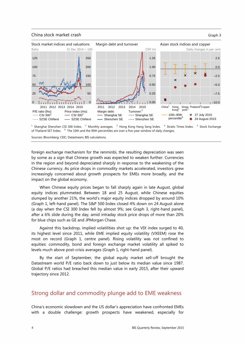
almost one third of its value between 12 June and 8 July (Graph 3, left-hand panel). The adjustment was even more dramatic for the Shenzhen Stock Exchange (SZSE) ChiNext small technology company index, which plunged by 40% over the same period.
The preceding run-up in Chinese equity prices was driven by increased trading activity and a build-up of leverage, which accelerated as the central bank eased monetary policy (Graph 3, centre panel). Combined daily turnover averaged CNY 1.8 trillion ($300 billion) in the month up to 12 June, around six times the 2014 average and exceeding that of the US stock market. This was fuelled by over 56 million new trading accounts opened predominantly by retail investors in the first half of 2015. Broker-intermediated margin trading reached CNY 2.2 trillion ($360 billion) in early June, an almost sixfold increase from the year before, representing approximately 8% of tradable market capitalisation. Increased leverage went hand in hand with rising valuations: the CSI 300 price/earnings ratio went up from 10 in mid-2014 to 21 in June 2015, while the P/E ratio on the ChiNext exchange peaked at 143 (Graph 3, left-hand panel). Turnover and leverage then plunged, reflecting new regulatory curbs and the rapid retreat of retail investors.
As concerns over Chinese equity market fundamentals persisted and authorities began scaling down their market-supporting measures, the volatility increasingly spilled over to other markets, especially in Asia. On 27 July, when the CSI 300 Index fell by 8.5% – its largest daily drop since 2007 – equity markets across Asia, and some commodity prices, suffered outsize drops (Graph 3, right-hand panel). In late July and early August, equity prices in China and elsewhere briefly stabilised.
This respite was short-lived. Concerns about China’s growth outlook took centre stage as the People’s Bank of China (PBoC) on 11 August announced major changes to its foreign exchange policy (see detailed discussion below). While the measures were officially described as a step towards a more market-oriented
Renewed Greek turmoil
In basis points Graph 2
Greek CDS spreads1 Flight to safety2 Limited contagion1
1 Sovereign US dollar-denominated credit default swaps (CDS); complete restructuring clauses. 2 Based on daily observations between 1 April 2015 to 2 September 2015.
Sources: Bloomberg; Markit; BIS calculations.
0
2,500
5,000
7,500
10,000
Feb 15 Apr 15 Jun 15 Aug 15
2-year 5-year 10-year
–14
–7
0
7
14
–3,000 –1,500 0 1,500 3,000Change in Greek 5-year CDS1
Cha
nge
in 1
0y g
ov’t
bon
d yi
eld
R2 = 0.15
R2 = 0.14
Switzerland Germany
0
1,750
3,500
5,250
7,000
70
105
140
175
210
Feb 15 Apr 15 Jun 15 Aug 15
5-year CDS spreads:Rhs:Greece (lhs) Italy
PortugalSpain
4 BIS Quarterly Review, September 2015
foreign exchange mechanism for the renminbi, the resulting depreciation was seen by some as a sign that Chinese growth was expected to weaken further. Currencies in the region and beyond depreciated sharply in response to the weakening of the Chinese currency. As price drops in commodity markets accelerated, investors grew increasingly concerned about growth prospects for EMEs more broadly, and the impact on the global economy.
When Chinese equity prices began to fall sharply again in late August, global equity indices plummeted. Between 18 and 25 August, while Chinese equities slumped by another 21%, the world’s major equity indices dropped by around 10% (Graph 1, left-hand panel). The S&P 500 Index closed 4% down on 24 August alone (a day when the CSI 300 Index fell by almost 9%; see Graph 3, right-hand panel), after a 6% slide during the day, amid intraday stock price drops of more than 20% for blue chips such as GE and JPMorgan Chase.
Against this backdrop, implied volatilities shot up: the VIX index surged to 40, its highest level since 2011, while EME implied equity volatility (VXEEM) rose the most on record (Graph 1, centre panel). Rising volatility was not confined to equities: commodity, bond and foreign exchange market volatility all spiked to levels much above post-crisis averages (Graph 1, right-hand panel).
By the start of September, the global equity market sell-off brought the Datastream world P/E ratio back down to just below its median value since 1987. Global P/E ratios had breached this median value in early 2015, after their upward trajectory since 2012.
Strong dollar and commodity plunge add to EME weakness
China’s economic slowdown and the US dollar’s appreciation have confronted EMEs with a double challenge: growth prospects have weakened, especially for
China stock market crash Graph 3
Stock market indices and valuations Margin debt and turnover Asian stock indices and copper Ratio 31 Dec 2014 = 100 CNY trn Daily changes in per cent
1 Shanghai Shenzhen CSI 300 Index. 2 Monthly averages. 3 Hong Kong Hang Seng Index. 4 Straits Times Index. 5 Stock Exchange of Thailand SET Index. 6 The 10th and the 90th percentiles are over a five-year window of daily changes.
Sources: Bloomberg; CEIC; Datastream; BIS calculations.
0
25
50
75
100
125
0
50
100
150
200
250
2011 2012 2013 2014 2015
CSI 3001
SZSE ChiNext
P/E ratio (lhs):CSI 3001
SZSE ChiNext
Price index (rhs):
0.00
0.25
0.50
0.75
1.00
1.25
2011 2012 2013 2014 2015
Shanghai SEShenzhen SE
Margin debt:Shanghai SEShenzhen SE
Turnover:2
–10.0
–7.5
–5.0
–2.5
0.0
2.5
China1 Hong Singa- Thailand5Copper Kong3 pore4
10th–90th percentile6
27 July 201524 August 2015
BIS Quarterly Review, September 2015 5
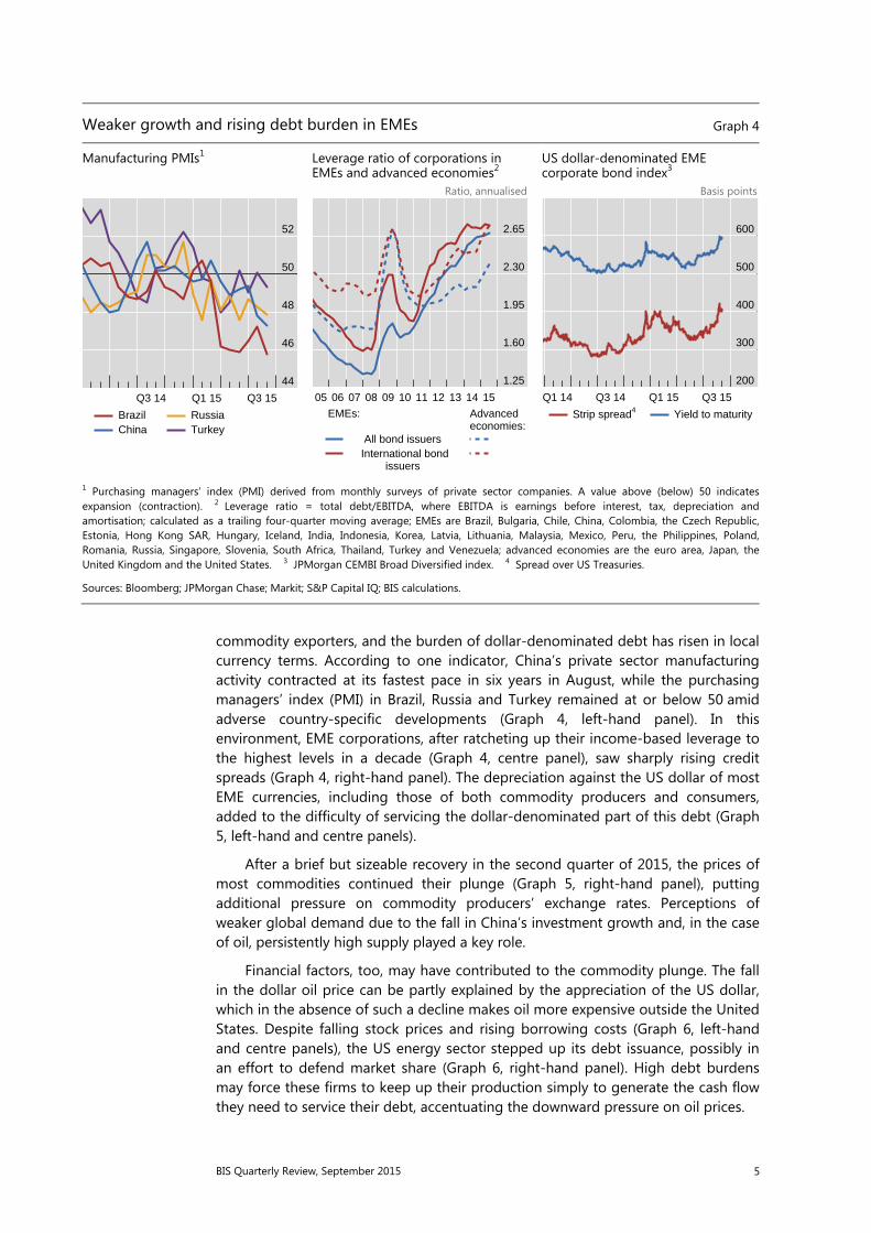
commodity exporters, and the burden of dollar-denominated debt has risen in local currency terms. According to one indicator, China’s private sector manufacturing activity contracted at its fastest pace in six years in August, while the purchasing managers’ index (PMI) in Brazil, Russia and Turkey remained at or below 50 amid adverse country-specific developments (Graph 4, left-hand panel). In this environment, EME corporations, after ratcheting up their income-based leverage to the highest levels in a decade (Graph 4, centre panel), saw sharply rising credit spreads (Graph 4, right-hand panel). The depreciation against the US dollar of most EME currencies, including those of both commodity producers and consumers, added to the difficulty of servicing the dollar-denominated part of this debt (Graph 5, left-hand and centre panels).
After a brief but sizeable recovery in the second quarter of 2015, the prices of most commodities continued their plunge (Graph 5, right-hand panel), putting additional pressure on commodity producers’ exchange rates. Perceptions of weaker global demand due to the fall in China’s investment growth and, in the case of oil, persistently high supply played a key role.
Financial factors, too, may have contributed to the commodity plunge. The fall in the dollar oil price can be partly explained by the appreciation of the US dollar, which in the absence of such a decline makes oil more expensive outside the United States. Despite falling stock prices and rising borrowing costs (Graph 6, left-hand and centre panels), the US energy sector stepped up its debt issuance, possibly in an effort to defend market share (Graph 6, right-hand panel). High debt burdens may force these firms to keep up their production simply to generate the cash flow they need to service their debt, accentuating the downward pressure on oil prices.
Weaker growth and rising debt burden in EMEs Graph 4
Manufacturing PMIs1 Leverage ratio of corporations in EMEs and advanced economies2
US dollar-denominated EME corporate bond index3
Ratio, annualised Basis points
1 Purchasing managers’ index (PMI) derived from monthly surveys of private sector companies. A value above (below) 50 indicatesexpansion (contraction). 2 Leverage ratio = total debt/EBITDA, where EBITDA is earnings before interest, tax, depreciation andamortisation; calculated as a trailing four-quarter moving average; EMEs are Brazil, Bulgaria, Chile, China, Colombia, the Czech Republic, Estonia, Hong Kong SAR, Hungary, Iceland, India, Indonesia, Korea, Latvia, Lithuania, Malaysia, Mexico, Peru, the Philippines, Poland, Romania, Russia, Singapore, Slovenia, South Africa, Thailand, Turkey and Venezuela; advanced economies are the euro area, Japan, the United Kingdom and the United States. 3 JPMorgan CEMBI Broad Diversified index. 4 Spread over US Treasuries.
Sources: Bloomberg; JPMorgan Chase; Markit; S&P Capital IQ; BIS calculations.
44
46
48
50
52
Q3 14 Q1 15 Q3 15
BrazilChina
RussiaTurkey
1.25
1.60
1.95
2.30
2.65
05 06 07 08 09 10 11 12 13 14 15
All bond issuers International bond issuers
EMEs: Advancedeconomies:
200
300
400
500
600
Q1 14 Q3 14 Q1 15 Q3 15
Strip spread4 Yield to maturity

6 BIS Quarterly Review, September 2015
Against this backdrop, a number of emerging market economy and commodity-exporting advanced economy central banks eased monetary policy,
Commodities resume their decline amid EME weakness Graph 5
Exchange rates of commodity producers1
Exchange rates of commodity-consuming EMEs1
Commodity rout continues2
31 Dec 2014 = 100 31 Dec 2014 = 100
1 US dollars per unit of local currency. A decline indicates a depreciation of the local currency. 2 Changes in spot prices.
Sources: Bloomberg; Datastream; BIS calculations.
Financial factors contribute to commodities plunge Graph 6
Energy sector stocks Energy sector corporate credit spreads4
Oil sector debt issuance in the United States5
2 June 2014 = 100 Ratio Basis points Basis points USD bn
1 S&P 500 equity index. 2 MSCI European Economic and Monetary Union equity index. 3 MSCI Emerging Markets equity index. 4 Option-adjusted spreads on an index of investment grade non-sovereign debt. The EME energy sector index consists of both investment grade and high-yield non-sovereign debt. For the US and euro area energy sector indices, March 2015 data are computed based on the end-February 2015 index constituents and their respective weights. 5 Sum of debt offering amounts by companies in the United States, excluding Chevron and Exxon.
Sources: Bank of America Merrill Lynch; Bloomberg; Datastream; S&P Capital IQ.
70
80
90
100
110
Feb 15 Apr 15 Jun 15 Aug 15
Australian dollarBrazilian realCanadian dollarIndonesianrupiah
Mexican pesoNorwegian kroneRussian roubleSouth Africanrand
70
80
90
100
110
Feb 15 Apr 15 Jun 15 Aug 15
Chinese renminbiHungarian forintIndian rupeeKorean won
Polish zlotySingaporedollarTurkish lira
WTI
Nickel
Copper
Wheat
Soybean
Gold
–30 –20 –10 0
% change from 29 May to 2 Sep 2015
25
40
55
70
85
100
0.6
0.7
0.8
0.9
1.0
1.1
2014 2015
Lhs:Energy sector
Rhs:Energy sector /overall index:
United States1
Euro area2
EMEs3
100
200
300
400
500
600
70
105
140
175
210
245
2014 2015Energy sector:Rhs:
Lhs:
All sectors: United States Euro area EMEs
0
12
24
36
48
60
10 11 12 13 14 15
BIS Quarterly Review, September 2015 7
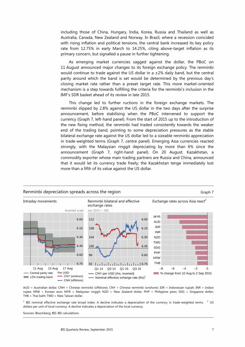
including those of China, Hungary, India, Korea, Russia and Thailand as well as Australia, Canada, New Zealand and Norway. In Brazil, where a recession coincided with rising inflation and political tensions, the central bank increased its key policy rate from 12.75% in early March to 14.25%, citing above-target inflation as its primary concern, but signalled a pause in further tightening.
As emerging market currencies sagged against the dollar, the PBoC on 11 August announced major changes to its foreign exchange policy. The renminbi would continue to trade against the US dollar in a ±2% daily band, but the central parity around which the band is set would be determined by the previous day’s closing market rate rather than a preset target rate. This more market-oriented mechanism is a step towards fulfilling the criteria for the renminbi’s inclusion in the IMF’s SDR basket ahead of its review in late 2015.
This change led to further ructions in the foreign exchange markets. The renminbi slipped by 2.8% against the US dollar in the two days after the surprise announcement, before stabilising when the PBoC intervened to support the currency (Graph 7, left-hand panel). From the start of 2015 up to the introduction of the new fixing method, the renminbi had traded consistently towards the weaker end of the trading band, pointing to some depreciation pressures as the stable bilateral exchange rate against the US dollar led to a sizeable renminbi appreciation in trade-weighted terms (Graph 7, centre panel). Emerging Asia currencies reacted strongly, with the Malaysian ringgit depreciating by more than 6% since the announcement (Graph 7, right-hand panel). On 20 August, Kazakhstan, a commodity exporter whose main trading partners are Russia and China, announced that it would let its currency trade freely; the Kazakhstan tenge immediately lost more than a fifth of its value against the US dollar.
Renminbi depreciation spreads across the region Graph 7
Intraday movements Renminbi bilateral and effective exchange rates
Exchange rates across Asia react2
Inverted scale Jan 2014 = 100
AUD = Australian dollar; CNH = Chinese renminbi (offshore); CNY = Chinese renminbi (onshore); IDR = Indonesian rupiah; INR = Indian rupee; KRW = Korean won; MYR = Malaysian ringgit; NZD = New Zealand dollar; PHP = Philippine peso; SDG = Singapore dollar;THB = Thai baht; TWD = New Taiwan dollar.
1 BIS nominal effective exchange rate broad index. A decline indicates a depreciation of the currency in trade-weighted terms. 2 US dollars per unit of local currency. A decline indicates a depreciation of the local currency.
Sources: Bloomberg; BIS; BIS calculations.
6.00
6.15
6.30
6.45
6.60
6.75
11 Aug 13 Aug 17 Aug
Central parity rate±2% trading band CNY (onshore)
CNH (offshore)
Per USD:
92
96
100
104
108
112 6.00
6.15
6.30
6.45
6.60
6.75
Q1 14 Q3 14 Q1 15 Q3 15
CNY per USD (rhs, inverted)Nominal effective exhange rate (lhs)1
THB
KRW
PHP
SDG
TWD
NZD
INR
IDR
AUD
MYR
–8 –6 –4 –2 0
% change from 10 Aug to 2 Sep 2015

8 BIS Quarterly Review, September 2015
Diverging monetary policies continue to drive markets
Diverging monetary policies have continued to be an important driver for markets over the past few months. With policy rates close to zero, the Bank of Japan and the ECB continued their respective asset purchase programmes, seeking to stimulate economic activity and lift inflation closer to target (Graph 8, left-hand panel). At the same time, the US Federal Reserve and the Bank of England continued to prepare market participants for an eventual increase in their policy rates.
In particular, the Federal Reserve’s efforts in this direction have been ongoing for some time, thus keeping US forward interest rates persistently above those in the euro area and elsewhere (Graph 8, centre panel). But macroeconomic upsets and bouts of market turbulence have prompted investors to scale back their expectations for near-term rate hikes. For example, whereas prices of federal funds futures contracts at the beginning of 2015 implied an 80% probability that the target rate would have been raised by September, and a 90% probability that it would have happened by December, these probabilities had fallen to around 32% and 58%, respectively, by 2 September (Graph 8, right-hand panel). These estimated probabilities dropped sharply twice during the quarter. On 8 July, they fell to 21% and 54%, respectively, shortly after the Greek referendum and on a day when the Shanghai equity index plummeted by 6%. After recovering in subsequent weeks, they again slid in late August following the extreme turbulence in global equity markets.
Although the timing of the Federal Reserve’s first move has become more uncertain, interest rate differentials between the United States and many other countries have remained wide, with important consequences for foreign exchange markets. In particular, except for a brief hiatus in the second quarter of 2015, the US
Diverging monetary policy outlook Graph 8
Central bank asset purchases Forward interest rate curves3 Fed rate hike probabilities4 USD bn USD bn Per cent Per cent
1 Holdings under the Securities Market Programme, the Asset-Backed Securities Purchase Programme, Covered Bond Purchase Programmes 1, 2 and 3 and the Public Sector Purchase Programme. 2 Outright purchases of Japanese government bonds. 3 For the United States, 30-day federal funds rate futures; for the euro area, three-month Euribor futures. 4 Based on Bloomberg implied probabilities from fed funds futures.
Sources: Bloomberg; Datastream.
210
280
350
420
490
560
1,320
1,440
1,560
1,680
1,800
1,920
Jan 14 Jul 14 Jan 15 Jul 15
ECB1Lhs:
Bank of Japan2Rhs:
0.0
0.4
0.8
1.2
1.6
2015 2016 2017
02 Mar 2015 01 Jun 2015 02 Sep 2015
United States: Euro area:
15
30
45
60
75
90
May 15 Jul 15
September 2015December 2015
Fed funds target rate above 0–0.25%range by:

BIS Quarterly Review, September 2015 9
dollar has been on an appreciating trend since mid-2014. The influence of interest rate differentials on the dollar was particularly stark with regard to the euro: as the difference between US and core euro area interest rates began to widen again in the third quarter of 2015, the dollar resumed its strengthening path against the euro (Graph 9, left-hand panel). Towards the end of the period, as US short-term rates edged down, the euro recovered somewhat.
Interest rate differentials also affected the behaviour of investors and borrowers. With interest rates at or near record lows in the euro area, fixed income investors increasingly turned to higher-yielding dollar assets. For example, flows into European exchange-traded funds linked to US bonds surged. In the first half of this year, such flows amounted to $4.8 billion, as compared with $4.0 billion in the entire year of 2014 and $3.4 billion in 2013 (Graph 9, centre panel). For their part, firms in the United States increasingly issued euro-denominated debt to benefit from the low borrowing costs. In the second quarter of 2015, total gross issuance of euro-denominated debt by US non-financial corporations amounted to €30 billion, surpassing even the brisk issuance of the previous two quarters (Graph 9, right-hand panel; see also “Highlights of global financing flows”, BIS Quarterly Review, September 2015). With ongoing ECB asset purchases weighing on the yields of core euro area government debt, yield-starved European investors have welcomed the rising supply of corporate debt.
Bond yields stuck at low levels
Long-term government bond yields in advanced economies edged lower to levels not far from the troughs reached early in the year, following sharp but brief increases in the second quarter. The yield on 10-year German government bonds, which peaked at just below 1% in early June 2015, had eased back to around
Markets adjust to widening interest rate differentials Graph 9
Diverging monetary policy outlook and the dollar
Inflow of fixed income European ETFs with exposure to the United States1
US corporate euro bond issuance
Percentage points USD bn EUR bn
1 Quarterly flows; ETFs = exchange-traded funds. 2 A decrease on an inverted scale indicates euro depreciation.
Sources: Bloomberg; Markit; national data; BIS international debt securities statistics.
0.0
0.2
0.4
0.6
0.8 1.1
1.2
1.3
1.4
1.5
Jan 14 Jul 14 Jan 15 Jul 15
2-yr spread: US Treasury–bund (lhs)USD per EUR (rhs, inverted)2
0.0
0.6
1.2
1.8
2.4
Q1 13 Q1 14 Q1 15
0
6
12
18
24
2010 2011 2012 2013 2014 2015
10 BIS Quarterly Review, September 2015
Box 1
Volatility and evaporating liquidity during the bund tantrum Ryan Riordan and Andreas Schrimpf
Volatility in German bond markets spiked during May–June 2015 (Graph A, top left-hand panel). Historical volatility, computed from daily maximum and minimum prices, was higher in June 2015 than during any other period over the past four years. Intraday volatility measures indicate even higher stress levels (Graph A, top right-hand panel). Bonds with very long maturities showed the highest intraday volatility, while bonds of shorter maturities were also affected, but to a lesser extent. Intraday data are taken from the Euro-MTS inter-dealer platform, the main wholesale electronic trading venue for German government bonds.
The “bund tantrum”, as some have termed the spike in German bond volatility on 7 May 2015, is especially puzzling. Yields on long-term bonds surged 21 basis points intraday, peaking at 80 basis points, but ended the day where they had been at the previous day’s close, at 59 basis points. While the dynamics differed, such large intraday moves bore some resemblance to the US Treasury “flash rally” on 15 October 2014, during which yields suddenly fell by nearly 30 basis points before recovering by the close of trading. Unlike the 3 June spike in bund yields, which followed the release of an ECB statement on the euro area economic outlook and led to a repricing of inflation expectations, the market break on 7 May does not appear to have been related to the release of any particular information. One trigger factor might have been an unwinding of positions by leveraged directional investors in fixed income derivatives markets. In anticipation of the ECB’s asset purchase programme, trades speculating on a continued decline in rates had become relatively crowded, according to some reports. In such circumstances, even minor news might have sufficed to turn the market’s direction.
A common explanation for why prices in fixed income markets have become so volatile is that market liquidity has deteriorated. Indeed, measures of market liquidity computed using firm prices that are immediately executable support the conjecture that strained market liquidity conditions are at least partly to blame for the increased volatility. The cost of immediately executable transactions in the bund market increased in the period around the bund tantrum. The increase in the bid-ask spread (Graph A, bottom left-hand panel), defined as the difference between the best available buy price (bid) and the best available sale price (offer) and expressed in basis points relative to the mid-quote, shows the increase in round-trip execution costs for small trades. Ultra-long-term bonds (those with more than 12½ years’ remaining maturity) exhibited the worst deterioration in bid-ask spreads, with a near doubling in the relative bid-ask spread from 40 to roughly 80 basis points. A second spike coincided with the ECB’s monetary policy press release on 3 June 2015. Some widening in bid-ask spreads around the release of pricing-relevant information is expected, as intermediaries widen quoted prices to reflect the increased risk that the market will move against them.
A more informative liquidity measure in this market is order book depth (Graph A, bottom right-hand panel), which also showed signs of deterioration over the period. Order book depth is defined as the total volume available for immediate transaction at the best available bid and offer prices. Lower order book depth means that even small increases in trading volume can lead to large price swings. Over the first half of 2015, depth in the order book of German bunds was low and fragile, which can potentially amplify price movements. The most striking decline was in the depth available in ultra-long-term bonds. Immediately executable depth fell by more than a third over the six-month period, from €25 million to roughly €16 million. Less depth makes it difficult to execute larger trades without moving prices; large trades may then lead to volatility spikes similar to those of May–June 2015.
A variety of factors may stand behind the overall decrease in market liquidity for German bonds. As part of a longer-term trend, liquidity has declined as intermediaries scale down their inventory holdings of fixed income assets (see eg Committee on the Global Financial System, “Market-making and proprietary trading: industry trends, drivers and policy implications”, CGFS Papers, no 52, November 2014). Some observers have also suggested that the ECB’s Public Sector Purchase Programme (PSPP) in early 2015 may have further reduced the supply of tradable German bonds, which had already been fairly strained due to low issuance volumes in primary markets. As of 30 June, the ECB had purchased €46.3 billion of German bonds, representing roughly 6% of total German PSPP-eligible securities. This, in turn, reduced the availability of bonds for trading by intermediaries. In particular, the depth available in German bond markets appears to have fallen around the time of the announcement, and it continued to fall at and after the start of the PSPP. However, the effects were most pronounced, and appear to be

BIS Quarterly Review, September 2015 11
Volatility and liquidity during the bund tantrum Graph A
Realised volatility (2011–15)1, 2 Intraday realised volatility1, 3, 4 Per cent Per cent
Relative bid-ask spreads4, 5 Order book depth4, 6 Basis points Basis points EUR millions
The vertical lines show 7 May 2015, the date of the first outburst of the bund tantrum, and 3 June 2015, the date of the ECB policy announcement.
1 Realised volatility is calculated as the daily (maximum midpoint–minimum midpoint)/average price. Data are intradaily from the MTS Euro Benchmark Markets (MTS-EBM) for benchmark bonds only. 2 Data are from January 2011 to June 2015, aggregated to a weekly average. 3 Daily average from January 2015 to June 2015. 4 Data are intradaily from the MTS-EBM for benchmark bonds only for January–June 2015. Both panels show daily averages. 5 The bid-ask spread is calculated as (ask – bid) / mid and is expressed in basis points. 6 Depth is calculated as the (volume at bid + volume at ask)/2.
Source: MTS Euro Benchmark Markets.
permanent, in bonds of very long-term maturity. As the ECB’s PSPP did not buy large amounts of these securities, other factors such as the limited risk-bearing capacity of intermediaries may also have contributed to the decline.
Indicators are constructed from submitted limit orders for benchmark bonds during normal trading hours (8:00–17:30). Bonds with a remaining maturity from 2.5 to 7.5 years are classified as medium-term, those >7.5 to <= 12.5 years as long-term, and those >12.5 years as ultra-long-term bonds. Market liquidity generally refers to the ease with which a security can be bought or sold without affecting the asset’s price. This differs from funding liquidity, which refers to the ease with which investors can obtain funding for a position in a risky asset (see M Brunnermeier and L Pedersen, “Market liquidity and funding liquidity”, Review of Financial Studies, no 22(6), 2009, pp 2201–38). The two measures of liquidity discussed here, the bid-ask spread and order book depth at the best bid and ask, are directly measurable in our data and are continuously available throughout the trading day. They are representative of realisable liquidity in the overall market. On 22 January 2015, the ECB unveiled its programme for public sector asset purchases (PSPP), amounting to purchases worth roughly €60 billion per month between 9 March and at least September 2016. The weighted average remaining maturity of German bonds held by the ECB in the PSPP is roughly 6.78 years; see www.ecb.europa.eu/mopo/implement/omt/html/ index.en.html.
0.0
0.6
1.2
1.8
2.4
3.0
2011 2012 2013 2014 2015
0
2
4
6
8
10
Jan 15 Feb 15 Mar 15 Apr 15 May 15 Jun 15
6
7
8
9
10
30
45
60
75
90
Jan 15 Feb 15 Mar 15 Apr 15 May 15 Jun 15
Medium-termLhs:
Long-term Ultra-long-termRhs:
15
18
21
24
27
Jan 15 Feb 15 Mar 15 Apr 15 May 15 Jun 15
Medium-term Long-term Ultra-long-term
12 BIS Quarterly Review, September 2015
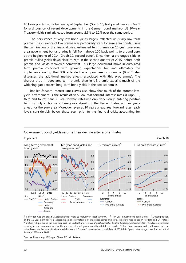
80 basis points by the beginning of September (Graph 10, first panel; see also Box 1 for a discussion of recent developments in the German bond market). US 10-year Treasury yields similarly eased from around 2.5% to 2.2% over the same period.
The persistence of very low bond yields largely reflected unusually low term premia. The influence of low premia was particularly stark for euro area bonds. Since the culmination of the financial crisis, estimated term premia on 10-year core euro area government bonds gradually fell from above 100 basis points to around zero at the beginning of 2014 (Graph 10, second panel). Since then, a prolonged slide in premia pulled yields down close to zero in the second quarter of 2015, before both premia and yields recovered somewhat. This large downward move in euro area term premia coincided with growing expectations for, and ultimately the implementation of, the ECB extended asset purchase programme (Box 2 also discusses the additional market effects associated with this programme). The sharper drop in euro area term premia than in US premia explains much of the widening gap between long-term bond yields in the two economies.
Implied forward interest rate curves also show that much of the current low-yield environment is the result of very low real forward interest rates (Graph 10, third and fourth panels). Real forward rates rise only very slowly, entering positive territory only at horizons three years ahead for the United States, and six years ahead for the euro area. Moreover, even at 10 years ahead, real forward rates reach levels considerably below those seen prior to the financial crisis, accounting for
Government bond yields resume their decline after a brief hiatus
In per cent Graph 10
Long-term government bond yields
Ten-year bond yields and term premium3
US forward curves4 Euro area forward curves4
1 JPMorgan GBI-EM Broad Diversified Index, yield to maturity in local currency. 2 Ten-year government bond yields. 3 Decomposition of the 10-year nominal yield according to an estimated joint macroeconomic and term structure model; see P Hördahl and O Tristani,“Inflation risk premia in the euro area and the United States”, International Journal of Central Banking, September 2014. Yields are expressed monthly in zero coupon terms; for the euro area, French government bond data are used. 4 Short-term nominal and real forward interest rates, based on the term structure model in note 1; “current” curves refer to end-August 2015 data, “pre-crisis averages” are for the period January 1999–June 2007.
Sources: Bloomberg; JPMorgan Chase; BIS calculations.
0.0
1.5
3.0
4.5
6.0
0.00
0.75
1.50
2.25
3.00
2013 2014 2015
EMEs1Lhs:
United StatesGermanyUnitedKingdomJapan
Rhs:2
–2.4
–1.2
0.0
1.2
2.4
3.6
09 10 11 12 13 14 15
Euro area:Yield
Term premium
United States:
–1.5
0.0
1.5
3.0
4.5
6.0
2 4 6 8 10Years ahead
CurrentPre-crisis average
Nominal:
–1.5
0.0
1.5
3.0
4.5
6.0
2 4 6 8 10Years ahead
CurrentPre-crisis average
Real:

BIS Quarterly Review, September 2015 13
almost all of the similarly large gap between current and pre-crisis nominal forward rates.
The behaviour of institutional investors may have played a role in explaining such unusually low yields. For example, as yields have come down, the duration of pension funds’ and insurance companies’ liabilities have lengthened, forcing them to step up their hedging activities. This has increased demand for long-term swaps, adding to the downward pressure on yields. Such self-reinforcing effects are likely to have been amplified in an environment where central banks continue to exert great demand for bonds, and where investors have persistently sought higher returns in longer-dated bonds.

14 BIS Quarterly Review, September 2015
Box 2
Dislocated markets
Over the past year, asset prices in some markets have persistently deviated from levels that would be consistent with the absence of arbitrage opportunities. Such distortions can occur when scarce funding or limited balance sheet capacity prevents investors from taking advantage of the resulting trading opportunities. This is often the case during financial crises. More recently, reduced market liquidity and central bank actions may have played a role. This box examines three prominent examples of dislocations.
Deviations from covered interest parity, which in the textbook view should normally be eliminated through riskless arbitrage, have been trending up for major currency pairs. The deviations were especially high for the Swiss franc after the Swiss National Bank discontinued its minimum exchange rate against the euro (Graph B, left-hand panel). Covered interest parity implies, among other things, that FX forward discount rates embedded in the price of FX swaps should be equal to the interest rate differentials between the currencies involved in the swap. Differences between money market rates and interest rates embedded in FX swaps often signal funding difficulties in one of the currencies. For instance, as unsecured US dollar funding markets became increasingly dysfunctional during the financial crisis, foreign banks with large dollar funding requirements increasingly turned to the FX swap market to obtain dollar funding, which in turn pushed FX swap-implied dollar interest rates far above dollar Libor rates.
The more recent spread widening between dollar interest rates derived from the FX swap market and those in the Libor market has also tended to favour the swap counterparty supplying dollars. However, this has probably reflected derivatives market imbalances, rather than funding difficulties of the kind seen during the height of the crisis. On the demand side, institutions such as non-US pension funds and insurance companies, which have large dollar asset positions but liabilities that are predominantly denominated in the local currency, may have ramped up their holdings of dollar bonds and their hedging activities. Such increased hedging needs may be linked to the
Dislocated asset prices Graph B
FX swap spread1 Euro area five-year inflation expectations measures
Swiss interest rates
Basis points Basis points Basis points Per cent Per cent
The vertical line in the left-hand and right-hand panels indicates 15 January 2015, when the Swiss National Bank discontinued its minimumexchange rate against the euro and lowered its policy rate to –0.75%. The vertical lines in the centre panel indicate 22 January 2015, whenthe ECB asset purchase programme was announced, and 9 March 2015, when purchases started.
1 Currencies against the US dollar; spread between the three-month FX swap-implied dollar rate and three-month US dollar Libor; the FX swap-implied rate is the implied cost of raising US dollars via FX swaps using the funding currency. 2 Based on French government bonds. 3 Estimated by regressing the weekly five-year break-even inflation rate on nominal yields with maturities ranging from two to 10 years during the period starting at the beginning of 2013.
Sources: Bloomberg; Datastream; BIS calculations.
0
50
100
150
200
0
8
16
24
32
Mar 14 Sep 14 Mar 15 Sep 15
CHFLhs:
EURJPY
Rhs:
–50
–25
0
25
50
0.0
0.4
0.8
1.2
1.6
Mar 14 Sep 14 Mar 15 Sep 15
Lhs:
Rhs:
Spread: inflation swap andbreak-even rateBreak-even rate2
Inflation implied by nominalyield curve3
–2
–1
0
1
2
Jul 14 Jan 15 Jul 15
3-month Libor10-year government bond yield10-year fixed mortgage lending rate

BIS Quarterly Review, September 2015 15
recent increase in FX volatility (Graph 1, right-hand panel). On the supply side, financial intermediaries’ ability to supply hedging instruments such as FX swaps has remained subdued, as they have significantly reduced their leverage since the financial crisis. As a result, they have been willing to devote balance sheet space in order to meet the increased demand for dollar swaps only in return for a considerable premium.
Such demand imbalances in FX swap markets have been reinforced as borrowers have reacted to changes in funding costs for dollars vis-à-vis other currencies. As major central banks outside the United States have ramped up their unconventional easing efforts, funding conditions have loosened considerably in key foreign currencies. As a result, US corporations have increasingly been issuing debt in foreign currency, including the euro (Graph 9, right-hand panel), and this may have further increased the demand for swapping into dollars.
Another dislocated market segment was that of inflation-linked bonds. Large gyrations in euro area break-even inflation rates (that is, inflation rates that would make the overall return on an inflation-linked bond equal to that of a comparable nominal bond) have highlighted the importance of liquidity premia for index-linked instruments. Because the nominal yield curve contains information about inflation expectations and risk premia, nominal interest rates can be used to track the variation in break-even inflation. The close relationship between the two broke down from the end of 2014 (Graph B, centre panel), as five-year break-even rates derived from inflation-linked bonds implied significantly lower inflation than the measure based on nominal yields only. This coincided with a fall in index-linked bond turnover reported by debt management agencies, suggesting that rising liquidity premia in index-linked bonds had driven their yields up and therefore pushed down measured break-even inflation rates. When the ECB announced and started implementing its expanded asset purchase programme, which explicitly included index-linked bonds, break-even inflation rates recovered sharply, possibly overshooting. The ECB actions therefore appear to have been perceived as significantly reducing illiquidity in the index-linked market segment, thus sharply reducing the liquidity premia required by investors. This suggests that variations in liquidity premia rather than shifts in inflation expectations were a key driver of euro area break-even inflation rates during this episode (Box 1 further discusses bond market liquidity developments, focusing on German government bond markets).
The negative policy rates introduced by several European central banks in 2014 and 2015 have also created distortions in some market segments, in particular when non-bank players have been involved. Across the affected countries, banks have so far been reluctant to pass on negative rates to retail depositors. This has exposed them to higher funding costs and additional interest rate risk. Swiss evidence suggests that banks have factored the lost revenue and hedging costs into the pricing of new mortgages, which led to an increase in the 10-year Swiss fixed mortgage rate, even as money market rates moved deeper into negative territory and government bond yields fell (Graph B, right-hand panel).
See eg N Baba and F Packer, “From turmoil to crisis: dislocations in the FX swap market before and after the failure of Lehman Brothers”,Journal of International Money and Finance, no 28(8), 2009, pp 1350–74.

BIS Quarterly Review, September 2015 17
Highlights of global financing flows1
The BIS, in cooperation with central banks and monetary authorities worldwide, compiles and disseminates data on activity in international financial markets. It uses these data to compile indicators of global liquidity conditions and early warning indicators of financial crisis risks. This chapter analyses recent trends in these indicators. It also summarises the latest data for international banking markets, available up to March 2015, and for international debt securities, available up to June 2015. A box provides more detail on domestic and foreign currency positions vis-à-vis China during the first quarter of 2015.
Takeaways
Global liquidity conditions were strong in the early months of 2015 forborrowers in advanced economies, but signs of weakening were apparentfor emerging market economies (EMEs). International financing inadvanced economies was marked by especially strong growth in bank andcapital market financing in euros. At the same time, international banklending and securities financing slowed or reversed for a number of EMEs,notably China and Russia.
At end-March 2015, financing of non-bank borrowers in US dollars outsidethe United States totalled $9.6 trillion, while financing of non-banks ineuros outside the euro area came to $2.8 trillion.
Global cross-border claims of BIS reporting banks continued to expand inearly 2015, rising by $748 billion in exchange rate-adjusted terms betweenend-December 2014 and end-March 2015.
International debt securities issuance remained strong, with net issuance of$225 billion in the first quarter of 2015 and $219 billion in the second.
Euro-denominated cross-border claims and claims on the euro area surgedduring the first quarter of 2015. About half of this euro-denominatedincrease went to non-bank borrowers and about half came from lendersinside the euro area. Greece was a notable exception: cross-border lending
1 This article was prepared by Ben Cohen ([email protected]) and Cathérine Koch ([email protected]). Statistical support was provided by Stephan Binder, Sebastian Goerlich, Branimir Gruić and Jeff Slee.

18 BIS Quarterly Review, September 2015
to residents of the country mostly denominated in euros fell by $22 billion between end-December 2014 and end-March 2015.
Cross-border bank lending to EMEs contracted by $52 billion on anexchange rate-adjusted basis in the first quarter of 2015.
Lending to China declined for the second consecutive quarter, slowing theannual growth rate to almost zero.
Cross-border claims on Russia and Ukraine saw another quarterly decline,accelerating their annual rates of contraction to a respective 29% and 48%.
Net debt securities issuance by advanced economy borrowers expanded atthe fastest pace since before the Great Financial Crisis of 2007–09, totalling$247 billion in the first half of 2015. EME borrowers, meanwhile, issued$137 billion in the first half, net of repayments, a notably slower growthrate than in the previous three years.
Early warning indicators point to continued vulnerability associated withdebt overhangs in key EMEs.
Recent developments in the international bank and debt markets
Despite bouts of volatility in securities and commodity markets (see “A wave of further easing”, BIS Quarterly Review, March 2015), international financial activity strengthened in the early months of 2015. According to the BIS locational banking statistics (LBS),2 international bank claims grew by almost 6%3 from the first quarter of 2014 to the first quarter of 2015 (Graph 1, top panel), and by close to 3% in Q1 2015 alone. Claims on non-banks increased by $626 billion in the first quarter of 2015, adjusted for breaks and exchange rates, while claims on banks rose by $218 billion. Meanwhile, as reported by the BIS international debt securities statistics (IDS),4 net issuance continued to grow at the steady pace seen since the end of the Great Financial Crisis (Graph 1, bottom panel). Net issuance totalled $188 billion in the first quarter of 2015 and $198 billion in the second, compared with $509 billion for the whole of 2014.
2 The LBS are structured according to the location of banking offices and capture the activity of all internationally active banking offices in the reporting country regardless of the nationality of the parent bank. Banks record their positions on an unconsolidated basis, including those vis-à-vis their own offices in other countries. International claims here include all BIS reporting banks’ cross-border claims and local claims in foreign currency. For the latest enhancements to the BIS international banking statistics, see S Avdjiev, P McGuire and P Wooldridge, “Enhanced data to analyse international banking”, BIS Quarterly Review, September 2015.
3 Annual percentage changes are calculated as the sum of exchange rate- and break-adjusted changes over the preceding four quarters divided by the amount outstanding one year earlier.
4 The BIS defines IDS as securities issued by non-residents in all markets. A debt security will be classified as IDS if any one of the following characteristics is different from the country of residence of the issuer: country where the security is registered, law governing the issue, or market where the issue is listed. See B Gruić and P Wooldridge, “Enhancements to the BIS debt securities statistics”, BIS Quarterly Review, December 2012. The IDS feature a breakdown by both the nationality and residence of the issuer, along with further dimensions such as type, sector, currency and maturity, on a quarterly basis.
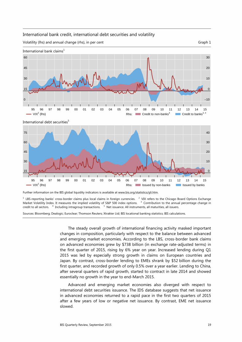
BIS Quarterly Review, September 2015 19
The steady overall growth of international financing activity masked important changes in composition, particularly with respect to the balance between advanced and emerging market economies. According to the LBS, cross-border bank claims on advanced economies grew by $738 billion (in exchange rate-adjusted terms) in the first quarter of 2015, rising by 6% year on year. Increased lending during Q1 2015 was led by especially strong growth in claims on European countries and Japan. By contrast, cross-border lending to EMEs shrank by $52 billion during the first quarter, and recorded growth of only 0.5% over a year earlier. Lending to China, after several quarters of rapid growth, started to contract in late 2014 and showed essentially no growth in the year to end-March 2015.
Advanced and emerging market economies also diverged with respect to international debt securities issuance. The IDS database suggests that net issuance in advanced economies returned to a rapid pace in the first two quarters of 2015 after a few years of low or negative net issuance. By contrast, EME net issuance slowed.
International bank credit, international debt securities and volatility
Volatility (lhs) and annual change (rhs), in per cent Graph 1
International bank claims1
International debt securities5
Further information on the BIS global liquidity indicators is available at www.bis.org/statistics/gli.htm.
1 LBS-reporting banks’ cross-border claims plus local claims in foreign currencies. 2 VIX refers to the Chicago Board Options Exchange Market Volatility Index. It measures the implied volatility of S&P 500 index options. 3 Contribution to the annual percentage change incredit to all sectors. 4 Including intragroup transactions. 5 Net issuance. All instruments, all maturities, all issuers.
Sources: Bloomberg; Dealogic; Euroclear; Thomson Reuters; Xtrakter Ltd; BIS locational banking statistics; BIS calculations.
0
15
30
45
60
–10
0
10
20
30
95 96 97 98 99 00 01 02 03 04 05 06 07 08 09 10 11 12 13 14 15
Rhs:VIX2 (lhs) Credit to non-banks3 Credit to banks3, 4
15
30
45
60
75
0
10
20
30
40
95 96 97 98 99 00 01 02 03 04 05 06 07 08 09 10 11 12 13 14 15
Rhs:VIX2 (lhs) Issued by non-banks Issued by banks

20 BIS Quarterly Review, September 2015
Global credit to the non-financial sector, by currency Graph 2
Amounts outstanding1 (USD trn) Annual change (in per cent)
Credit denominated in US dollars (USD)
Credit denominated in euros (EUR)
Credit denominated in Japanese yen (JPY)
Further information on the BIS global liquidity indicators is available at www.bis.org/statistics/gli.htm.
1 Amounts outstanding at quarter-end. Amounts denominated in currencies other than USD are converted to USD at the exchange rate prevailing at end-March 2015. 2 Credit to non-financial borrowers residing in the United States/euro area/Japan. National financial accounts are adjusted using BIS banking and securities statistics to exclude credit denominated in non-local currencies. 3 Excluding debt securities issued by special purpose vehicles and other financial entities controlled by non-financial parents. EUR-denominated debt securities exclude those issued by institutions of the European Union. 4 Loans by LBS-reporting banks to non-bank borrowers, including non-bank financial entities, comprise cross-border plus local loans. For countries that are not LBS-reporting countries, local loans in USD/EUR/JPY are estimated as follows: for China, local loans in foreign currencies are from national data and are assumed to be composed of 80% USD, 10% EUR and 10% JPY; for other non-reporting countries, local loans to non-banks are set equal to LBS-reporting banks’ cross-border loans to banks in the country (denominated in USD/EUR/JPY), on the assumption that these funds are onlent to non-banks.
Sources: IMF, International Financial Statistics; Datastream; BIS debt securities statistics; BIS locational banking statistics.
0
12
24
36
48
00 01 02 03 04 05 06 07 08 09 10 11 12 13 14 15
–30
–15
0
15
30
00 02 04 06 08 10 12
–30
–15
0
15
30
2013 2014 2015
0
10
20
30
40
00 01 02 03 04 05 06 07 08 09 10 11 12 13 14 15
–30
–15
0
15
30
00 02 04 06 08 10 12
–30
–15
0
15
30
2013 2014 2015
0
10
20
30
40
00 01 02 03 04 05 06 07 08 09 10 11 12 13 14 15
Credit to residents2
Of which: Credit to government
Debt securities3
Loans4
Credit to non-residents:
–30
–15
0
15
30
00 02 04 06 08 10 12
Debt securities3
Loans4
Credit to non-residents:
–30
–15
0
15
30
2013 2014 2015
Credit toresidents2
BIS Quarterly Review, September 2015 21
The remainder of this chapter reviews these developments in more detail, focusing on the BIS statistics on international banking and international debt securities, and on the BIS global liquidity indictors (GLIs). It concludes with a brief review of recent trends in credit growth and debt service ratios (DSRs) in the major advanced and emerging market economies.
Global foreign currency credit to the non-financial sector
Global credit to the non-resident, non-financial sector in US dollars and euros continued to grow faster than credit to non-financial residents of the United States and the euro area (Graph 2).
According to the GLIs, credit in US dollars to non-bank borrowers outside the United States totalled $9.6 trillion at the end of Q1 2015. Excluding non-bank financial borrowers from this figure, the total of credit in US dollars to non-financial borrowers comes to $7.8 trillion (Graph 2, top left-hand panel). Bank loans in dollars to these non-financial borrowers stood at $5.3 trillion, an annual increase of almost 10%, while securities issued amounted to $2.5 trillion, lifting the annual growth rate of the outstanding stock to 9% (Graph 2, top right-hand panel). Both grew faster than did US dollar credit to non-financial residents of the United States (which rose 4%). These growth rates have been remarkably stable for several years.
At end-March 2015, credit in euros to non-bank borrowers outside the euro area totalled $2.8 trillion. Excluding non-bank financials again, the total of credit in euros to non-financial borrowers is $2.1 trillion, comprising $1.2 trillion in bank loans and $915 billion in debt securities (Graph 2, middle left-hand panel). The outstanding stock of euro-denominated bonds issued by non-resident non-financials jumped by almost 14% on an annual basis, driven in part by a sharp net increase in euro-denominated debt issuance by US non-financial corporations. Bank lending in euros to non-financials outside the euro area, which had contracted for much of 2013, started rising again in the first quarter of 2014 and rose by 10% in the year to March 2015 (Graph 2, middle right-hand panel). Both banking and securities credit growth in euros to the non-resident non-financial sector far outpaced the growth in credit to residents in the non-financial sector of the euro area, which grew 4%.
Credit in yen to non-financial borrowers outside Japan, at end-March 2015, comprised $347 billion in bank lending and $66 billion in debt securities. Bank lending grew by 4% in the year to March 2015, whereas the stock of outstanding debt securities contracted by 9.3% over the same period (Graph 2, bottom panels).
Global cross-border credit
The expansion of global cross-border lending that began in the second quarter of 2014 picked up in the first three months of 2015. According to the LBS, the cross-border claims of BIS reporting banks increased by $748 billion between end-
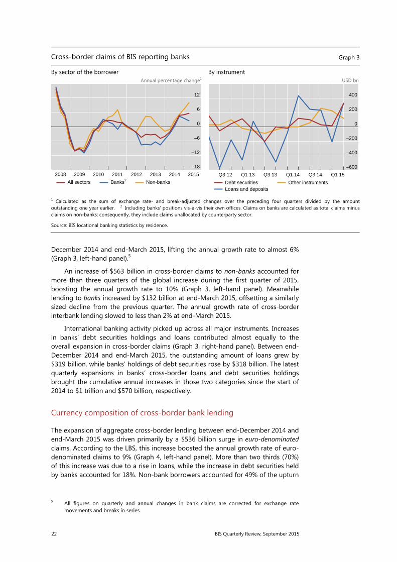
22 BIS Quarterly Review, September 2015
December 2014 and end-March 2015, lifting the annual growth rate to almost 6% (Graph 3, left-hand panel).5
An increase of $563 billion in cross-border claims to non-banks accounted for more than three quarters of the global increase during the first quarter of 2015, boosting the annual growth rate to 10% (Graph 3, left-hand panel). Meanwhile lending to banks increased by $132 billion at end-March 2015, offsetting a similarly sized decline from the previous quarter. The annual growth rate of cross-border interbank lending slowed to less than 2% at end-March 2015.
International banking activity picked up across all major instruments. Increases in banks’ debt securities holdings and loans contributed almost equally to the overall expansion in cross-border claims (Graph 3, right-hand panel). Between end-December 2014 and end-March 2015, the outstanding amount of loans grew by $319 billion, while banks’ holdings of debt securities rose by $318 billion. The latest quarterly expansions in banks’ cross-border loans and debt securities holdings brought the cumulative annual increases in those two categories since the start of 2014 to $1 trillion and $570 billion, respectively.
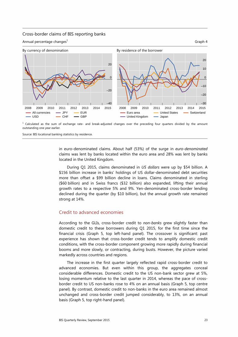
Currency composition of cross-border bank lending
The expansion of aggregate cross-border lending between end-December 2014 and end-March 2015 was driven primarily by a $536 billion surge in euro-denominated claims. According to the LBS, this increase boosted the annual growth rate of euro-denominated claims to 9% (Graph 4, left-hand panel). More than two thirds (70%) of this increase was due to a rise in loans, while the increase in debt securities held by banks accounted for 18%. Non-bank borrowers accounted for 49% of the upturn
5 All figures on quarterly and annual changes in bank claims are corrected for exchange rate movements and breaks in series.
Cross-border claims of BIS reporting banks Graph 3
By sector of the borrower By instrument Annual percentage change1 USD bn
1 Calculated as the sum of exchange rate- and break-adjusted changes over the preceding four quarters divided by the amountoutstanding one year earlier. 2 Including banks’ positions vis-à-vis their own offices. Claims on banks are calculated as total claims minusclaims on non-banks; consequently, they include claims unallocated by counterparty sector.
Source: BIS locational banking statistics by residence.
–18
–12
–6
0
6
12
2008 2009 2010 2011 2012 2013 2014 2015
All sectors Banks2 Non-banks
–600
–400
–200
0
200
400
Q3 12 Q1 13 Q3 13 Q1 14 Q3 14 Q1 15
Debt securitiesLoans and deposits
Other instruments
BIS Quarterly Review, September 2015 23
in euro-denominated claims. About half (53%) of the surge in euro-denominated claims was lent by banks located within the euro area and 28% was lent by banks located in the United Kingdom.
During Q1 2015, claims denominated in US dollars were up by $54 billion. A $156 billion increase in banks’ holdings of US dollar-denominated debt securities more than offset a $99 billion decline in loans. Claims denominated in sterling ($60 billion) and in Swiss francs ($32 billion) also expanded, lifting their annual growth rates to a respective 5% and 9%. Yen-denominated cross-border lending declined during the quarter (by $10 billion), but the annual growth rate remained strong at 14%.
Credit to advanced economies
According to the GLIs, cross-border credit to non-banks grew slightly faster than domestic credit to these borrowers during Q1 2015, for the first time since the financial crisis (Graph 5, top left-hand panel). The crossover is significant: past experience has shown that cross-border credit tends to amplify domestic credit conditions, with the cross-border component growing more rapidly during financial booms and more slowly, or contracting, during busts. However, the picture varied markedly across countries and regions.
The increase in the first quarter largely reflected rapid cross-border credit to advanced economies. But even within this group, the aggregates conceal considerable differences. Domestic credit to the US non-bank sector grew at 5%, losing momentum relative to the last quarter in 2014, whereas the pace of cross-border credit to US non-banks rose to 4% on an annual basis (Graph 5, top centre panel). By contrast, domestic credit to non-banks in the euro area remained almost unchanged and cross-border credit jumped considerably, to 13%, on an annual basis (Graph 5, top right-hand panel).
Cross-border claims of BIS reporting banks
Annual percentage changes1 Graph 4
By currency of denomination By residence of the borrower
1 Calculated as the sum of exchange rate- and break-adjusted changes over the preceding four quarters divided by the amountoutstanding one year earlier.
Source: BIS locational banking statistics by residence.
–40
–20
0
20
2008 2009 2010 2011 2012 2013 2014 2015
All currenciesUSD
JPYCHF
EURGBP
–30
–20
–10
0
10
20
2008 2009 2010 2011 2012 2013 2014 2015
Euro areaUnited Kingdom
United StatesJapan
Switzerland

24 BIS Quarterly Review, September 2015
Turning to cross-border bank credit vis-à-vis all sectors, LBS data suggest that the trends that had been developing since 2014 continued in the first quarter. The annual growth rates of cross-border claims, which had been negative for several years after the crisis before turning positive in 2014, remained in positive territory. Growth rates were particularly high for Japan (16%), the euro area (9%), the United Kingdom (8%) and Switzerland (5%), while cross-border claims on the United States remained virtually unchanged between March 2014 and 2015 (Graph 4, right-hand panel).
Cross-border claims on all borrowers in the euro area (including intra-euro area claims and all sectors) rose by $418 billion during Q1 2015, spurring the annual growth rate to almost 9%. As pointed out by the LBS, this was the highest quarterly increase in absolute terms since Q1 2008 (Graph 4, right-hand panel). Interbank activity contributed slightly less than borrowing by non-banks to this figure. Banks from the euro area accounted for a little less than half of the increase, while banks located in the United Kingdom accounted for 35% of this increase. A $153 billion upsurge in lending to Germany fuelled the overall increase in cross-border claims on the euro area. France also saw a significant ($124 billion) rise in overall cross-
Global bank credit to non-banks, by borrower region
Banks’ cross-border credit plus local credit in all currencies1 Graph 5
All countries2 United States Euro area USD trn Per cent USD trn Per cent USD trn Per cent
Emerging Asia Latin America Emerging Europe USD trn Per cent USD trn Per cent USD trn Per cent
Further information on the BIS global liquidity indicators is available at www.bis.org/statistics/gli.htm.
1 Cross-border claims of LBS-reporting banks plus local claims of all banks. Local claims are from national financial accounts and include credit extended by the central bank to the government. 2 Sample of 52 countries. 3 Amounts outstanding at quarter-end. Amounts denominated in currencies other than the US dollar are converted to US dollars at the exchange rate prevailing at end-March 2015.
Sources: IMF, International Financial Statistics; BIS locational banking statistics; BIS calculations.
0
25
50
75
100
–24
–12
0
12
24
01 03 05 07 09 11 13 15
0
5
10
15
20
–24
–12
0
12
24
01 03 05 07 09 11 13 15
0
5
10
15
20
–24
–12
0
12
24
01 03 05 07 09 11 13 15
0
6
12
18
24
–50
–25
0
25
50
01 03 05 07 09 11 13 15
Cross-border creditLocal credit
Amounts outstanding3 (lhs):
0.0
0.8
1.6
2.4
3.2
–40
–20
0
20
40
01 03 05 07 09 11 13 15
Cross-border creditLocal credit
Annual change (rhs):
0.0
0.3
0.6
0.9
1.2
–40
–20
0
20
40
01 03 05 07 09 11 13 15

BIS Quarterly Review, September 2015 25
border claims on its residents. By contrast, lending to Spain, Italy, Ireland and Portugal remained virtually unchanged.
Cross-border bank lending also increased to borrowers in European countries outside the euro area (Graph 4, right-hand panel). Cross-border claims on Switzerland surged by $60 billion between end-December 2014 and end-March 2015, again on an exchange rate-adjusted basis. About 83% of the increase reflects interbank activity. With reporting banks’ cross-border liabilities to Switzerland having declined by $24 billion during the same period, their overall net claims on Switzerland increased by more than $86 billion. Claims on Denmark and Sweden saw similar increases. Cross-border claims on Denmark jumped by $27 billion and those on Sweden surged by $13 billion. In both cases, about two thirds of the increases involved cross-border claims on the banking sector.
Greece was a notable exception to the overall pattern of increased lending in Europe. According to the LBS, the cross-border claims of internationally active banks on Greece dropped by $22 billion during Q1 2015. As a result, the annual rate of contraction reached 28% at end-March 2015. Figures from the CBS6 on an immediate counterparty basis tell a similar story, revealing a $31 billion (€26 billion) decline in international lending to Greek residents7 during the first quarter of 2015 (Graph 6).
Most of the decline was accounted for by $26 billion (or €21 billion) of lending to Greek banks. The outstanding stock of consolidated international claims on Greek banks (on an immediate counterparty basis) amounted to $2.5 billion (€2.3 billion) at end-March 2015. International claims on the Greek official sector
6 The CBS classify exposures according to the nationality of banks (ie according to the location of
banks’ headquarters), not according to the location of the office in which they are booked. Banks consolidate their inter-office positions and report only their claims on unrelated borrowers without providing a currency breakdown. As a consequence, exchange rate-adjusted changes are not available in the consolidated banking statistics. Claims are reported on an immediate counterparty basis (ie according to the location of the borrowing entity) and on an ultimate risk basis (according to where the ultimate debtor is headquartered, taking account of guarantees and other risk transfers).
7 This calculation corrects for the depreciation of the euro against the US dollar by assuming that all claims are denominated in euros.
Banks’ international claims on Greece, by sector Graph 6
EUR bn
Source: BIS consolidated banking statistics (immediate counterparty).
0
25
50
75
100
125
2009 2010 2011 2012 2013 2014 2015
All sectors Non-bank private sector Banks Official sector
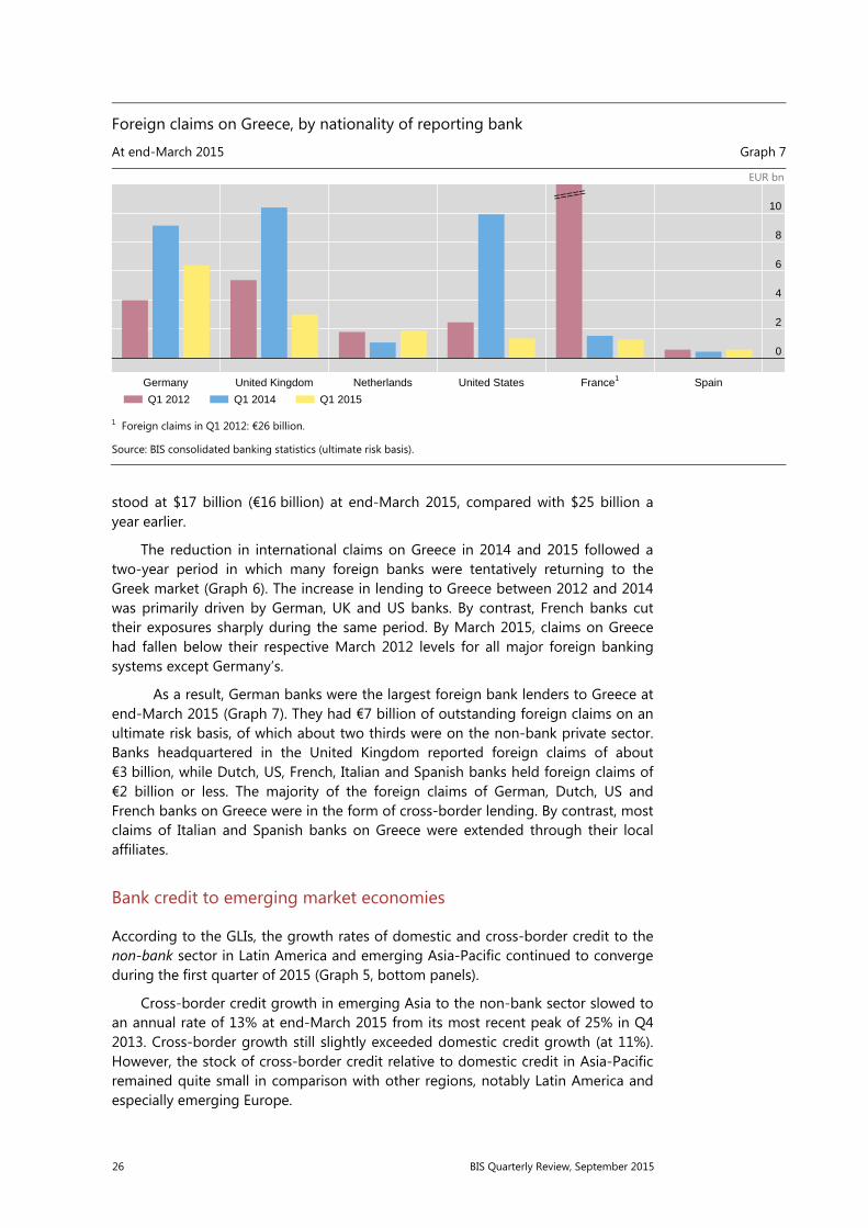
26 BIS Quarterly Review, September 2015
stood at $17 billion (€16 billion) at end-March 2015, compared with $25 billion a year earlier.
The reduction in international claims on Greece in 2014 and 2015 followed a two-year period in which many foreign banks were tentatively returning to the Greek market (Graph 6). The increase in lending to Greece between 2012 and 2014 was primarily driven by German, UK and US banks. By contrast, French banks cut their exposures sharply during the same period. By March 2015, claims on Greece had fallen below their respective March 2012 levels for all major foreign banking systems except Germany’s.
As a result, German banks were the largest foreign bank lenders to Greece at end-March 2015 (Graph 7). They had €7 billion of outstanding foreign claims on an ultimate risk basis, of which about two thirds were on the non-bank private sector. Banks headquartered in the United Kingdom reported foreign claims of about €3 billion, while Dutch, US, French, Italian and Spanish banks held foreign claims of €2 billion or less. The majority of the foreign claims of German, Dutch, US and French banks on Greece were in the form of cross-border lending. By contrast, most claims of Italian and Spanish banks on Greece were extended through their local affiliates.
Bank credit to emerging market economies
According to the GLIs, the growth rates of domestic and cross-border credit to the non-bank sector in Latin America and emerging Asia-Pacific continued to converge during the first quarter of 2015 (Graph 5, bottom panels).
Cross-border credit growth in emerging Asia to the non-bank sector slowed to an annual rate of 13% at end-March 2015 from its most recent peak of 25% in Q4 2013. Cross-border growth still slightly exceeded domestic credit growth (at 11%). However, the stock of cross-border credit relative to domestic credit in Asia-Pacific remained quite small in comparison with other regions, notably Latin America and especially emerging Europe.
Foreign claims on Greece, by nationality of reporting bank
At end-March 2015 Graph 7
EUR bn
1 Foreign claims in Q1 2012: €26 billion.
Source: BIS consolidated banking statistics (ultimate risk basis).
0
2
4
6
8
10
Germany United Kingdom Netherlands United States France1 Spain
=====
Q1 2012 Q1 2014 Q1 2015

BIS Quarterly Review, September 2015 27
Cross-border credit to non-banks in Latin America saw another quarterly increase between end-December 2014 and end-March 2015, with annual growth rising to 7% but remaining below the almost unchanged domestic growth rate of 12%.
Overall, domestic credit to non-banks in emerging Europe8 stagnated during the first quarter of 2015, whereas cross-border credit declined by 10%.
Data from the LBS show that, between end-December 2014 and end-March 2015, cross-border bank lending to all sectors (banks and non-banks) in EMEs declined for a second consecutive quarter, following two years of considerable growth. Cross-border claims on EMEs contracted by $52 billion in exchange rate-adjusted terms during the first quarter of 2015, slowing the year-on-year growth rate to below 1%.
Continuing the trend observed in recent years, claims on China drove the aggregate quarterly change in cross-border lending to EMEs as a whole and emerging Asia in particular. During the first quarter of 2015, cross-border lending to emerging Asia fell by $53 billion, slowing its annual growth rate to almost zero after several years of strong growth. This decline in claims on emerging Asia was more than accounted for by a $56 billion fall in cross-border claims on China, which brought down the year-on-year growth in claims on that country to zero (Graph 8, left-hand panel). The latest contraction in lending to China, which was driven by a $64 billion decline in cross-border claims on banks, took the outstanding stock of claims on the country to $963 billion at end-March 2015. The box below looks more closely at shifts in dollar- and renminbi-denominated banking flows to and from China in the early months of 2015.
8 The set of countries that constitute “emerging Europe” in the GLIs includes Ukraine but not Russia. The LBS definition of “emerging Europe” includes both countries. More details on cross-border positions vis-à-vis emerging Europe, including Russia, are provided below, drawn from the LBS.
Cross-border claims on selected emerging market economies
Annual percentage change1 Graph 8
Emerging Asia Latin America Emerging Europe
1 Calculated as the sum of exchange rate- and break-adjusted changes over the preceding four quarters divided by the amountoutstanding one year earlier.
Source: BIS locational banking statistics by residence.
–25
0
25
50
75
2011 2012 2013 2014 2015
IndonesiaChina
IndiaKorea
–15
0
15
30
45
2011 2012 2013 2014 2015
MexicoBrazil
Chile
–50
–25
0
25
50
2011 2012 2013 2014 2015
RussiaTurkey
Ukraine

28 BIS Quarterly Review, September 2015
Capital flowed out of China through BIS reporting banks in Q1 2015 Robert N McCauley
Capital outflows from China are much discussed, with many analyses focused on a seeming decline in official foreign exchange reserves. Yet measuring capital outflows with declines in foreign exchange reserves neglects valuation changes due to dollar/euro movements. Moreover, official reserves can be used to fund dollar investments in, for instance, new multilateral development banks.
However, BIS locational international banking statistics show a net $109 billion outflow in Q1 2015 from banks in China to banks outside China. This has put downward pressure on the renminbi and, given close currency management, on official reserves. This box shows how weakening incentives to hold long-renminbi positions resulted in the net outflow that took place both in foreign currency and in the renminbi in the first quarter. These results offer clues as to what may happen in the third quarter, during which China changed its exchange rate policy.
In the first quarter, the incentives for holding long-renminbi, short-dollar positions waned. First, the Chinese authorities continued the easing cycle that began in November by cutting administered deposit rates. And second, the renminbi was allowed to depreciate against the dollar from less than 6.2 per dollar to over 6.25 in mid-March. As a result, option-implied currency volatility rose. In short, the interest rate differential narrowed and the cost of insuring against further depreciation increased, reducing incentives for the long-renminbi position.
To clarify this point, consider a stylised Chinese multinational firm, with its balance sheet partly in China and partly outside. In China, the firm borrows and makes deposits in both renminbi and foreign currency. Its foreign currency debt at home exceeds its foreign currency deposits there. Outside China, it also has a larger foreign currency debt than foreign currency deposits, but more renminbi deposits than renminbi debt.
In response to reduced incentives, if the multinational sought to reduce its long-renminbi, short-foreign currency position, how would it have done so? The firm needs to reduce net foreign currency liabilities while shedding renminbi deposits. One place to adjust is within China. The People’s Bank of China (PBoC) reports that foreign currency deposits at banks in China banks grew by $83 billion in the first quarter while the increase in their foreign currency loans slowed to only $34 billion. Thus the multinational might have reduced its net foreign currency debt by building up foreign currency deposits in China. As a result, banks in China experienced a net inflow of $49 billion in foreign currency. If banks in China, in turn, placed their excess foreign currency funding with banks in the rest of the world, BIS reporting banks would experience a corresponding rise in liabilities to banks in China. And indeed, BIS reporting banks increased their liabilities to banks in China by $46 billion in the first quarter.
Alternatively, the firm could adjust its position outside China. For example, the treasurer could reduce renminbi deposits in an offshore bank. In fact, total renminbi deposits held in banks in Hong Kong SAR, Chinese Taipei, Singapore and Korea fell by $10 billion in Q1 2015 (Graph A). Or the treasurer could liquidate structured notes that are related to the renminbi/dollar rate that require his counterparty bank to hold renminbi as a hedge against fluctuations in the notes’ currency value. Such a liquidation would not show up in these non-bank deposit data. But fortunately, the PBoC now reports total renminbi deposits held by the rest of the world in banks in China. According to the PBoC, such deposits fell by $57 billion, which would reflect both the $10 billion reduction of renminbi deposits and lower bank demand for renminbi, whether arising from customer transactions or banks’ positioning of their own funds. Whatever its source, this $57 billion renminbi outflow accounts for the bulk of the $63 billion decline in claims on banks in China recorded by BIS reporting banks.
So, piling up foreign currency deposits in China ($49 billion), and reducing long-renminbi positions outside China ($57 billion), our stylised multinational could set off transactions that would lead to almost $109 billion in net outflows from banks in China. That much of the outflow was renminbi-denominated signifies progress in cross-border renminbi use – but also that this use has depended on favourable yield differentials and currency expectations.
Of course, reality is more complex than a single actor adjusting its renminbi/dollar position on both sides of the border. Non-banks in China actually borrowed a further $7 billion in the quarter from BIS reporting banks. This counts as a capital inflow, so that the net outflow from banks and non-banks in China was $102 billion in Q1 2015. And other entities, such as small and medium-sized enterprises in Hong Kong SAR and Chinese Taipei, have also entered long-renminbi, short-dollar positions and might also have unwound them in Q1 2015.
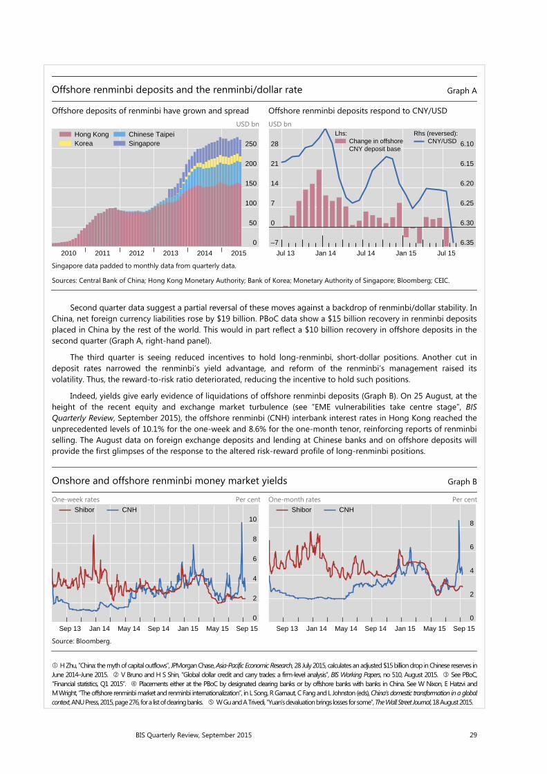
BIS Quarterly Review, September 2015 29
Offshore renminbi deposits and the renminbi/dollar rate Graph A
Offshore deposits of renminbi have grown and spread Offshore renminbi deposits respond to CNY/USD USD bn USD bn
Singapore data padded to monthly data from quarterly data.
Sources: Central Bank of China; Hong Kong Monetary Authority; Bank of Korea; Monetary Authority of Singapore; Bloomberg; CEIC.
Second quarter data suggest a partial reversal of these moves against a backdrop of renminbi/dollar stability. In China, net foreign currency liabilities rose by $19 billion. PBoC data show a $15 billion recovery in renminbi deposits placed in China by the rest of the world. This would in part reflect a $10 billion recovery in offshore deposits in the second quarter (Graph A, right-hand panel).
The third quarter is seeing reduced incentives to hold long-renminbi, short-dollar positions. Another cut in deposit rates narrowed the renminbi’s yield advantage, and reform of the renminbi’s management raised its volatility. Thus, the reward-to-risk ratio deteriorated, reducing the incentive to hold such positions.
Indeed, yields give early evidence of liquidations of offshore renminbi deposits (Graph B). On 25 August, at the height of the recent equity and exchange market turbulence (see “EME vulnerabilities take centre stage”, BIS Quarterly Review, September 2015), the offshore renminbi (CNH) interbank interest rates in Hong Kong reached the unprecedented levels of 10.1% for the one-week and 8.6% for the one-month tenor, reinforcing reports of renminbi selling. The August data on foreign exchange deposits and lending at Chinese banks and on offshore deposits will provide the first glimpses of the response to the altered risk-reward profile of long-renminbi positions.
Onshore and offshore renminbi money market yields Graph B
One-week rates Per cent One-month rates Per cent
Source: Bloomberg.
H Zhu, “China: the myth of capital outflows”, JPMorgan Chase, Asia-Pacific Economic Research, 28 July 2015, calculates an adjusted $15 billion drop in Chinese reserves in June 2014–June 2015. V Bruno and H S Shin, “Global dollar credit and carry trades: a firm-level analysis”, BIS Working Papers, no 510, August 2015. See PBoC, “Financial statistics, Q1 2015”. Placements either at the PBoC by designated clearing banks or by offshore banks with banks in China. See W Nixon, E Hatzvi and M Wright, “The offshore renminbi market and renminbi internationalization”, in L Song, R Garnaut, C Fang and L Johnston (eds), China’s domestic transformation in a global context, ANU Press, 2015, page 276, for a list of clearing banks. W Gu and A Trivedi, “Yuan’s devaluation brings losses for some”, The Wall Street Journal, 18 August 2015.
0
50
100
150
200
250
2010 2011 2012 2013 2014 2015
Hong KongKorea
Chinese TaipeiSingapore
–7
0
7
14
21
28 6.10
6.15
6.20
6.25
6.30
6.35
Jul 13 Jan 14 Jul 14 Jan 15 Jul 15
Change in offshore CNY deposit base
Lhs:CNY/USD
Rhs (reversed):
0
2
4
6
8
10
Sep 13 Jan 14 May 14 Sep 14 Jan 15 May 15 Sep 15
Shibor CNH
0
2
4
6
8
Sep 13 Jan 14 May 14 Sep 14 Jan 15 May 15 Sep 15
Shibor CNH
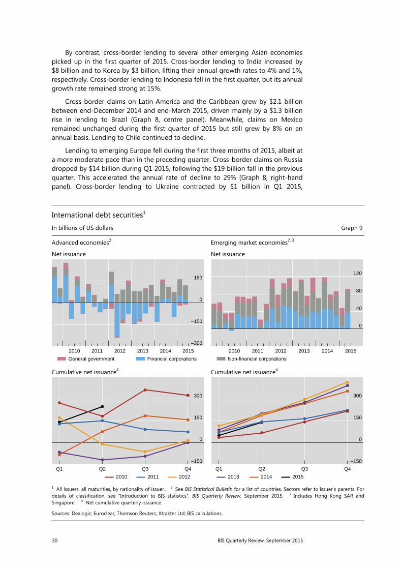
30 BIS Quarterly Review, September 2015
By contrast, cross-border lending to several other emerging Asian economies picked up in the first quarter of 2015. Cross-border lending to India increased by $8 billion and to Korea by $3 billion, lifting their annual growth rates to 4% and 1%, respectively. Cross-border lending to Indonesia fell in the first quarter, but its annual growth rate remained strong at 15%.
Cross-border claims on Latin America and the Caribbean grew by $2.1 billion between end-December 2014 and end-March 2015, driven mainly by a $1.3 billion rise in lending to Brazil (Graph 8, centre panel). Meanwhile, claims on Mexico remained unchanged during the first quarter of 2015 but still grew by 8% on an annual basis. Lending to Chile continued to decline.
Lending to emerging Europe fell during the first three months of 2015, albeit at a more moderate pace than in the preceding quarter. Cross-border claims on Russia dropped by $14 billion during Q1 2015, following the $19 billion fall in the previous quarter. This accelerated the annual rate of decline to 29% (Graph 8, right-hand panel). Cross-border lending to Ukraine contracted by $1 billion in Q1 2015,
International debt securities1
In billions of US dollars Graph 9
Advanced economies2 Emerging market economies2, 3
Net issuance Net issuance
Cumulative net issuance4 Cumulative net issuance4
1 All issuers, all maturities, by nationality of issuer. 2 See BIS Statistical Bulletin for a list of countries. Sectors refer to issuer’s parents. For details of classification, see “Introduction to BIS statistics”, BIS Quarterly Review, September 2015. 3 Includes Hong Kong SAR and Singapore. 4 Net cumulative quarterly issuance.
Sources: Dealogic; Euroclear; Thomson Reuters; Xtrakter Ltd; BIS calculations.
–300
–150
0
150
2010 2011 2012 2013 2014 2015
General government Financial corporations
0
40
80
120
2010 2011 2012 2013 2014 2015
Non-financial corporations
–150
0
150
300
Q1 Q2 Q3 Q4
2010 2011 2012
–150
0
150
300
Q1 Q2 Q3 Q4
2013 2014 2015

BIS Quarterly Review, September 2015 31
bringing the annual rate of decline to 48% at the end of March 2015. By contrast, cross-border lending to Turkey expanded by $4 billion, boosting its annual growth rate to 9%. In the meantime, cross-border claims on Hungary and the Czech Republic picked up marginally.
International debt securities
Net issuance in international debt securities markets grew to $225 billion in the first quarter of 2015 and $219 billion in the second (Graph 9). According to the IDS, at $444 billion, issuance in the first half of 2015 was 49% and 26% higher than in the second and first halves of 2014, respectively. The pace of net issuance in advanced economies, at $247 billion, ran well ahead of that of the last few years (Graph 9, bottom left-hand panel). Borrowers based in EMEs issued $137 billion, a slower pace than in recent years (Graph 9, bottom right-hand panel). Offshore centres and international organisations accounted for the remainder.
International debt securities1
Half-year net issuance, in billions of US dollars Graph 10
United States Euro area
Other advanced economies2 Emerging market economies2
1 Non-financial headquarters, by nationality of issuer. 2 See BIS Statistical Bulletin for a list of countries.
Sources: Dealogic; Euroclear; Thomson Reuters; Xtrakter Ltd; BIS calculations.
–40
0
40
80
2008 2009 2010 2011 2012 2013 2014 2015
–60
0
60
120
2008 2009 2010 2011 2012 2013 2014 2015
–40
0
40
80
2008 2009 2010 2011 2012 2013 2014 2015
EUR USD
–40
0
40
80
2008 2009 2010 2011 2012 2013 2014 2015
Other currencies
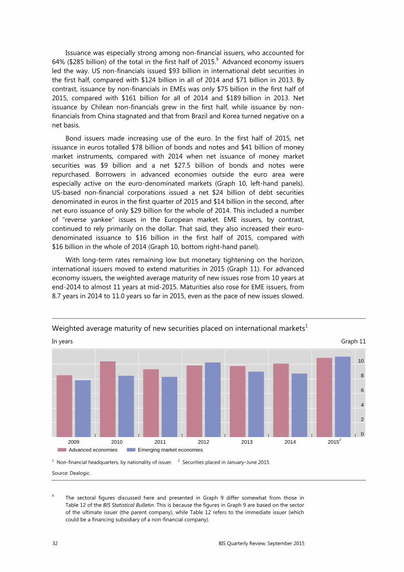
32 BIS Quarterly Review, September 2015
Issuance was especially strong among non-financial issuers, who accounted for 64% ($285 billion) of the total in the first half of 2015.9 Advanced economy issuers led the way. US non-financials issued $93 billion in international debt securities in the first half, compared with $124 billion in all of 2014 and $71 billion in 2013. By contrast, issuance by non-financials in EMEs was only $75 billion in the first half of 2015, compared with $161 billion for all of 2014 and $189 billion in 2013. Net issuance by Chilean non-financials grew in the first half, while issuance by non-financials from China stagnated and that from Brazil and Korea turned negative on a net basis.
Bond issuers made increasing use of the euro. In the first half of 2015, net issuance in euros totalled $78 billion of bonds and notes and $41 billion of money market instruments, compared with 2014 when net issuance of money market securities was $9 billion and a net $27.5 billion of bonds and notes were repurchased. Borrowers in advanced economies outside the euro area were especially active on the euro-denominated markets (Graph 10, left-hand panels). US-based non-financial corporations issued a net $24 billion of debt securities denominated in euros in the first quarter of 2015 and $14 billion in the second, after net euro issuance of only $29 billion for the whole of 2014. This included a number of “reverse yankee” issues in the European market. EME issuers, by contrast, continued to rely primarily on the dollar. That said, they also increased their euro-denominated issuance to $16 billion in the first half of 2015, compared with $16 billion in the whole of 2014 (Graph 10, bottom right-hand panel).
With long-term rates remaining low but monetary tightening on the horizon, international issuers moved to extend maturities in 2015 (Graph 11). For advanced economy issuers, the weighted average maturity of new issues rose from 10 years at end-2014 to almost 11 years at mid-2015. Maturities also rose for EME issuers, from 8.7 years in 2014 to 11.0 years so far in 2015, even as the pace of new issues slowed.
9 The sectoral figures discussed here and presented in Graph 9 differ somewhat from those in Table 12 of the BIS Statistical Bulletin. This is because the figures in Graph 9 are based on the sector of the ultimate issuer (the parent company), while Table 12 refers to the immediate issuer (which could be a financing subsidiary of a non-financial company).
Weighted average maturity of new securities placed on international markets1
In years Graph 11
1 Non-financial headquarters, by nationality of issuer. 2 Securities placed in January–June 2015.
Source: Dealogic.
0
2
4
6
8
10
2009 2010 2011 2012 2013 2014 20152
Advanced economies Emerging market economies

BIS Quarterly Review, September 2015 33
Early warning indicators for domestic banking crisis signal risks ahead1 Table 1
Credit-to-GDP gap2 Property price gap3 Debt service ratio4 Debt service ratio if interest rates rise by 250 bp4, 5
Asia6 18.3 10.4 2.0 4.3
Australia 1.6 1.5 0.7 4.5
Brazil 15.7 –5.2 4.6 6.3
Canada 6.5 6.3 1.7 5.5
China 25.4 –6.3 5.8 9.1
Central and eastern Europe7
–11.2 7.1 1.2 2.7
France 5.7 –11.7 1.4 4.5
Germany –5.9 9.7 –1.8 0.1
Greece –7.4 4.6
India –3.4 2.1 3.2
Italy –9.8 –17.2 0.8 3.0
Japan 5.2 13.3 –2.2 0.6
Korea 3.4 4.2 0.1 3.8
Mexico 6.0 –4.0 0.3 0.9
Netherlands –14.7 –19.2 1.6 6.5
Nordic countries8 1.5 2.6 1.7 5.9
Portugal –29.7 7.6 –0.5 2.9
South Africa –2.1 –6.2 –0.9 0.4
Spain –39.1 –26.6 –2.2 0.8
Switzerland 9.3 11.6 0.4 3.6
Turkey 16.6 4.1 5.7
United Kingdom –29.0 –3.1 –1.7 1.2
United States –12.5 0.9 –1.8 0.7
Legend Credit/GDP gap>10 Property gap>10 DSR>6 DSR>6
2≤Credit/GDP gap≤10 4≤DSR≤6 4≤DSR≤6
1 Thresholds for red cells are chosen by minimising false alarms conditional on capturing at least two thirds of the crises over a cumulative three-year horizon. A signal is correct if a crisis occurs in any of the three years ahead. The noise is measured by the wrong predictions outside this horizon. Beige cells for the credit-to-GDP gap are based on guidelines for countercyclical capital buffers under Basel III. Beige cells for the DSR are based on critical thresholds if a two-year forecast horizon is used. For a derivation of critical thresholds for credit-to-GDP gaps and property price gaps, see M Drehmann, C Borio and K Tsatsaronis, “Anchoring countercyclical capital buffers: the role of credit aggregates”, International Journal of Central Banking, vol 7(4), 2011. For DSRs, see M Drehmann and M Juselius, “Do debt service costs affect macroeconomic and financial stability?", BIS Quarterly Review, September 2012. Simple average for country aggregates. 2 Difference of the credit-to-GDP ratio from its long-run, real-time trend calculated with a one-sided Hodrick-Prescott (HP) filter using a smoothing factor of 400000, in percentage points. 3 Deviations of real residential property prices from their long-run trend calculated with a one-sided HP filter using a smoothing factor of 400000, in per cent. 4 For the DSR series and methodology, see www.bis.org/statistics/dsr.htm. Difference of DSRs from country-specific long-run averages since 1999 or later depending on data availability and when five-year average inflation fell below 10%, in percentage points. 5 Assuming that interest rates increase 2.5 percentage points and that all the other components of the DSR stay fixed. 6 Hong Kong SAR, Indonesia, Malaysia, the Philippines, Singapore and Thailand; excluding the Philippines and Singapore for the DSR and its forecast. 7 Bulgaria, the Czech Republic, Estonia, Hungary, Latvia, Lithuania, Poland, Romania and Russia; excluding the Czech Republic and Romania for the real property price gap; excluding Bulgaria, Estonia, Latvia, Lithuania and Romania for the DSR and its forecasts. 8 Finland, Norway and Sweden.
Sources: National data; BIS; BIS calculations.

34 BIS Quarterly Review, September 2015
Early warning indicators
Early warning indicators of banking stress pointed to risks arising from strong credit growth (Table 1). Credit-to-GDP gaps – the deviation of private sector credit from its long-term trend – were well above 10% in Brazil and China. This ratio was also above 10% for a number of countries that are not listed separately in Table 1, including Indonesia, Singapore and Thailand (these countries are included in the “Asia” category in line 1 of Table 1). In the past, two thirds of all readings above this threshold were followed by serious banking strains in the subsequent three years.10
Estimated debt service ratios also pointed to continuing risks.11 True, despite rapid credit growth, low interest rates have kept DSRs around their long-term level in most countries. Even so, there were some notable exceptions: households and firms in Brazil, China and Turkey, for example, spent significantly more on servicing their debt than in the past. More generally, however, an increase in interest rates would push up DSRs in a number of EMEs, especially in Asia (Table 1, last column). It should be noted that the DSR impacts in Table 1 are “static” estimates – they assume an immediate pass-through of interest rate changes into DSRs, and do not take account of the ways in which borrowers and lenders would respond to interest rate movements by changing debt maturities, repaying their obligations or other measures.
10 See M Drehmann, C Borio and K Tsatsaronis, “Anchoring countercyclical capital buffers: the role of credit aggregates”, International Journal of Central Banking, vol 7(4), December 2011.
11 See M Drehmann, A Illes, M Juselius and M Santos, “How much income is used for debt payments? A new database for debt service ratios”, BIS Quarterly Review, September 2015.

BIS Quarterly Review, September 2015 35
Introduction to BIS statistics1
The BIS is expanding its statistics by publishing additional data, revamping how these data are disseminated and strengthening their policy orientation. This special feature briefly describes each BIS data set and explains how the statistics can be used for analysis.
The statistics published by the BIS are a unique source of information about the structure of and activity in the global financial system. They are compiled in cooperation with central banks and other national authorities and are designed to inform analysis of financial stability, international monetary spillovers and global liquidity. Some BIS statistics, in particular those on international banking, securities markets and derivatives activity, are part of special collections under the auspices of BIS-hosted committees of central banks. Other BIS statistics draw on national data but incorporate assumptions and estimations by BIS statisticians to construct specific measures, such as global liquidity indicators, aggregate credit figures, debt service ratios and effective exchange rates.
With this edition of the BIS Quarterly Review, the BIS is expanding its statistical offering. The BIS is releasing enhanced data on international banking, new series on government debt, and estimates of debt service ratios for selected sectors (see the related special features in this issue). Furthermore, the BIS is revamping how it disseminates data. The tables previously published in the statistical annex to the Review have been replaced with charts illustrating the latest developments.2 The tables have been redesigned in a new publication, the BIS Statistical Bulletin, and made accessible in a new dynamic web-based tool, the BIS Statistics Explorer.3
A key objective of this expansion is to promote the wider use of BIS statistics, especially for policy analysis. It builds on an international initiative to improve the availability of key information for policymakers to assess risks across countries. This
1 This article was prepared by the BIS Monetary and Economic Department. Questions about the article may be addressed to Christian Dembiermont ([email protected]) and Philip Wooldridge ([email protected]). Queries about BIS statistics may be addressed to [email protected].
2 Data behind all graphs published in the BIS Quarterly Review are available on the BIS website, from the right-hand panel of the BIS Quarterly Review homepage.
3 The BIS Statistical Bulletin is published quarterly at the same time as the BIS Quarterly Review. Data may have been revised or updated subsequent to the publication of the latest Bulletin. The latest data are available from the BIS website (www.bis.org/statistics/index.htm). A release calendar provides advance notice of data updates (www.bis.org/statistics/relcal.htm).
36 BIS Quarterly Review, September 2015
Data Gaps Initiative is endorsed by the G20 and overseen by the Inter-Agency Group of international organisations, of which the BIS is a member.4
This special feature briefly describes each BIS data set and explains how the statistics can be used for analysis. Each section corresponds to the section in the Bulletin where the respective statistics are published.
Locational banking statistics www.bis.org/statistics/about_banking_stats.htm
Under the auspices of the Committee on the Global Financial System (CGFS), the BIS compiles and publishes two sets of statistics on international banking activity: the locational banking statistics (LBS) and the consolidated banking statistics (CBS).
The LBS provide information about the currency composition of banks’ balance sheets and the geographical breakdown of their counterparties. They capture outstanding claims and liabilities of internationally active banks located in reporting countries against counterparties residing in more than 200 countries. Banks record their positions on an unconsolidated basis, including intragroup positions between offices of the same banking group. The data are compiled following principles that are consistent with balance of payments statistics. Currently banking offices located in 44 countries, including many offshore financial centres, report the LBS. The LBS capture around 95% of all cross-border interbank business.
The availability of a currency breakdown in the LBS, coupled with the reporting of breaks in series arising from changes in methodology, reporting practices or reporting population, enables the BIS to calculate break- and exchange rate- adjusted changes in amounts outstanding. Such adjusted changes approximate underlying flows during a quarter.5
Extension of domestic credit and external debt measures
The LBS complement monetary and credit aggregates by providing information on banks’ cross-border and foreign currency positions. Indeed, the LBS were first compiled in the 1960s to track the growth in US dollar deposits outside the United States. This was especially important in the 1960s and 1970s, when policymakers had concerns about the possible macroeconomic consequences of the expansion of the money supply through the so-called eurocurrency markets (international deposit and loan markets).
Nowadays, extending domestic credit aggregates and supplementing external debt measures are more important uses of the LBS. As international financial crises have shown, banks located abroad can be significant – and volatile – sources of credit. Therefore, the LBS can provide a useful signal regarding potential fragilities
4 The IAG comprises the BIS, the ECB, Eurostat, the IMF, the OECD, the United Nations and the World Bank. For more information about the G20 Data Gaps Initiative, see IMF-FSB (2009, 2015).
5 Adjusted changes may over- or underestimate underlying flows because adjusted changes may also be affected by changes in valuations, writedowns, the underreporting of breaks, and differences between the exchange rate on the transaction date and the quarterly average exchange rate used by the BIS to convert non-dollar amounts into US dollars.
BIS Quarterly Review, September 2015 37
in the financial system. In particular, the LBS can help monitor the build-up of vulnerabilities associated with cross-border and foreign currency bank credit. For example, studies using the LBS have found that cross-border bank credit tends to grow considerably faster than overall credit during the expansionary phase of the financial cycle and that international credit is often a major driver of domestic credit booms (see eg Avdjiev, McCauley and McGuire (2012) and Borio et al (2011)). Furthermore, the currency breakdown available in the LBS gives insights into international monetary policy spillovers and has been used to document the importance of European banks in US dollar intermediation outside the United States (Shin (2012)). Finally, the LBS can also be utilised to analyse potential mismatches in the currency and sectoral composition of external assets and liabilities.
Geography of international banking
The details available in the LBS shed light on the role of banks in the intermediation of international capital flows and the structure of their intermediation. They reveal not only the residence and sector of banks’ counterparties, but also the instruments and currencies in which banks transact and the residence and nationality of the banks. In short, the LBS help track how funds are transferred from sources in one country via banks to users in another. Various studies have used the LBS to analyse banks’ role in the transmission of shocks across countries via bank lending and funding (see eg Bernanke et al (2011) and Bruno and Shin (2015)).
The LBS are best suited for analysing interconnections at the country level: for example, the importance of intragroup positions in cross-border funding; the channelling of funds through offshore financial centres; or the recycling of the petrodollars of oil exporters (see eg von Peter (2007) and McGuire and Tarashev (2008)).
Understanding the drivers of bank flows between countries requires information about who makes the underlying economic decisions. Key decisions are typically made by the head office of a bank, and thus for financial stability analysis it is often more important to know the nationality of the bank than its location. The CBS, discussed in the next section, provide the most comprehensive information on foreign lending by bank nationality. The LBS complement the CBS by providing information that can be used to track banks’ cross-currency funding and investment patterns on a nationality basis (see eg Fender and McGuire (2010) and McGuire and von Peter (2012)). Recent enhancements to the LBS provide additional information by nationality (Avdjiev et al (2015)).
Consolidated banking statistics www.bis.org/statistics/about_banking_stats.htm
The CBS capture the worldwide consolidated positions of internationally active banking groups headquartered in reporting countries. The data include the claims of reporting banks’ foreign affiliates but exclude intragroup positions, similarly to the consolidation approach followed by banking supervisors. For example, the positions of a German bank’s subsidiary located in London – which in the LBS are included in the positions of banks in the United Kingdom – are consolidated in the

38 BIS Quarterly Review, September 2015
CBS with those of its parent and included in positions of German banks. Currently, banking groups from 31 countries report the CBS.
Like the LBS, the CBS are reported to the BIS at an aggregate (banking system) level rather than individual bank level. A central bank or another national authority collects data from internationally active banks in its jurisdiction, compiles national aggregates and then sends them to the BIS to calculate global aggregates. No currency breakdown is available for the CBS, and thus the BIS does not calculate adjusted changes. Comparisons of amounts outstanding between periods are thus affected by movements in exchange rates.6
The CBS are compiled in two different ways: by immediate counterparty and by ultimate risk. The immediate counterparty is the entity with whom the bank contracts to lend or borrow. Ultimate risk takes account of credit risk mitigants, such as collateral, guarantees and credit protection bought, that transfer the bank’s credit exposure from one counterparty to another. For example, suppose that a German bank extends a loan to a company in Mexico and the loan is guaranteed by a US bank. On an immediate counterparty basis, the German bank would report the loan as a claim on Mexico. On an ultimate risk basis, the loan would be reported as a claim on the United States because, if the company in Mexico were unable to meet its obligations, then ultimately the German bank would be exposed to the US bank that guaranteed the loan. Data on an ultimate risk basis are better measures of exposures than data on an immediate counterparty basis because risk transfers may create a significant wedge between the two.
Banks’ foreign exposures
The CBS are designed to analyse the exposure of internationally active banks of different nationalities to individual countries and sectors. Exposures can take many forms: for example, cross-border claims, local claims of banks’ foreign affiliates, derivatives, guarantees, or credit commitments. The CBS provide information on each of these, and the most appropriate measure of exposure will depend on the issue being analysed. The benchmark measure in the CBS is foreign claims, which capture credit to borrowers outside the bank’s home country, including credit extended by banks’ foreign affiliates (but excluding derivatives, guarantees and credit commitments).7 Foreign claims are the most comparable measure across banks of diverse nationalities because differences in accounting standards complicate the comparability of other measures of exposures, especially derivatives.
The CBS on an ultimate risk basis are widely used to gauge reporting banks’ exposures to different countries and sectors. For example, they have been used to measure foreign banks’ exposures to US borrowers on the eve of the Great Financial Crisis of 2007–09 (see eg Borio and Disyatat (2011)). Other studies have used the CBS to contrast the evolution of euro area banks’ sovereign portfolios with those of banks from the rest of the world (see eg Caruana and Avdjiev (2012)).
6 This complicates analysis of flows using the CBS: for instance, a depreciation of a given currency against the US dollar will result in a decline in the reported US dollar value of outstanding claims denominated in that currency (and an appreciation an increase in the reported value).
7 Foreign claims are the sum of cross-border and local claims, excluding claims on residents of the country where the bank is headquartered. In the CBS on an immediate counterparty basis, foreign claims are disaggregated into local claims denominated in local currencies and international claims, where international claims refer to cross-border claims plus local claims in foreign currencies.
BIS Quarterly Review, September 2015 39
Borrowers’ dependence on foreign bank creditors
From a borrower’s point of view, the CBS also provide information about the main bank creditors to a given economy. The CBS on an immediate counterparty basis can be used to assess the dependence of individual borrowing countries and regions on foreign bank creditors. For example, based on these data, Avdjiev, Kuti and Takáts (2012) found that the sharp contraction in cross-border bank lending to emerging market economies that occurred in 2011 was largely linked to the deteriorating health of euro area banks.
In addition, the CBS data have been used to examine the transmission of adverse liquidity shocks from major banking systems to emerging market economies during the Great Financial Crisis (Cetorelli and Goldberg (2011)). And the maturity breakdown available in the CBS on an immediate counterparty basis has been used to construct indicators measuring the vulnerability of emerging market economies to sudden capital withdrawals through the banking system (see eg BIS (2011)).
Debt securities statistics www.bis.org/statistics/about_securities_stats.htm
The BIS debt securities statistics capture borrowing in money and bond markets, distinguishing between international and domestic markets. International debt securities (IDS) are those issued in a market other than the local market of the country where the borrower resides (Gruić and Wooldridge (2012)). They encompass what market participants have traditionally referred to as foreign bonds and eurobonds. Domestic debt securities (DDS) are those issued by residents in their local market, regardless of the currency in which the securities are denominated. Total debt securities (TDS) sum these together as all debt securities issued by residents.
The BIS debt securities statistics are harmonised with the recommendations in the Handbook on Securities Statistics, which sets out an internationally agreed framework for classifying securities issues and holdings (BIS-ECB-IMF (2015)). IDS are compiled by the BIS from commercial data sources, in particular Dealogic, Euroclear, Thomson Reuters and Xtrakter; the BIS constructs aggregates from data on individual securities. DDS and TDS are compiled from national data sources using aggregated data. For some countries, national data are available for either DDS or TDS but not both; for this reason, DDS and TDS are not published for all countries. While conceptually TDS are the sum of IDS and DDS, the BIS does not calculate the missing series because it cannot control for potential double-counting: for example, individual securities that the BIS classifies as international may be included in the aggregated data on DDS.
As of end-March 2015, the BIS published IDS, DDS and TDS statistics for residents of 17 countries; IDS and DDS for a further 16 countries; IDS and TDS for 22 countries; and only IDS for 75 countries. The security-by-security information that underlies the IDS statistics enables the BIS to provide more details than are available in the DDS and TDS statistics (Box 1). Furthermore, the availability of DDS and TDS lags that of IDS by one quarter.
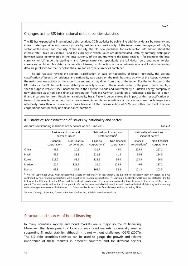
40 BIS Quarterly Review, September 2015
Structure and sources of bond financing
In many countries, money and bond markets are a major source of financing. Moreover, the development of local currency bond markets is generally seen as supporting financial stability, although it is not without challenges (CGFS (2007)). The BIS debt securities statistics can be used to gauge the growth and relative importance of these markets in different countries and for different sectors.
Box 1
Changes to the BIS international debt securities statistics
The BIS has expanded its international debt securities (IDS) statistics by publishing additional details by currency and interest rate type. Whereas previously data by residence and nationality of the issuer were disaggregated only by sector of the issuer and maturity of the security, the BIS now publishes, for each sector, information about the interest rate – fixed or variable – and the currency in which issues are denominated. Data by currency distinguish between issues denominated in the local currency of the country where the issuer resides – for example, the local currency for UK issuers is sterling – and foreign currencies, specifically the US dollar, euro and other foreign currencies combined. For data by nationality of issuer, no distinction is made between local and foreign currencies; data are published for the US dollar, the euro and all other currencies combined.
The BIS has also revised the sectoral classification of data by nationality of issuer. Previously, the sectoral classification of issuers by residence and nationality was based on the main business activity of the issuer. However, the main business activity of the issuer’s parent entity may differ from that of the issuer. For the full history of the IDS statistics, the BIS has reclassified data by nationality to refer to the ultimate sector of the parent. For example, a special purpose vehicle (SPV) incorporated in the Cayman Islands and controlled by a Russian energy company is now classified as a non-bank financial corporation from the Cayman Islands on a residence basis but as a non-financial corporation from Russia on a nationality basis. Table A below shows the impact of this reclassification on issuers from selected emerging market economies. Amounts for non-financial corporations are much larger on a nationality basis than on a residence basis because of the reclassification of SPVs and other non-bank financial corporations controlled by non-financial corporations.
IDS statistics: reclassification of issuers by nationality and sector
Amounts outstanding in billions of US dollars, at end-June 2015 Table A
Residence of issuer and sector of issuer
Nationality of parent and sector of issuer1
Nationality of parent and sector of parent2
Financial corporations3
Non-financial corporations
Financial corporations3
Non-financial corporations
Financial corporations3
Non-financial corporations
China 55.1 10.6 431.7 45.0 209.5 267.2
Brazil 55.9 38.1 211.8 41.3 98.6 154.5
Korea 118.2 55.6 123.6 56.4 113.5 66.5
Mexico 20.7 125.9 21.0 125.9 9.6 137.2
Russia 43.8 34.8 165.4 38.5 101.3 102.51 Prior to September 2015, when reclassifying issuers by nationality of their parent, the BIS did not reclassify them by sector, eg SPVs controlled by non-financial corporations were classified as financial corporations. 2 Starting in September 2015 and backdated for the full history of the IDS statistics, the BIS revised the sectoral classification of issuers on a nationality basis to refer to the sector of the issuer’sparent. The nationality and sector of the parent refer to the latest available information, and therefore historical data may not accurately reflect changes in who controls the issuer. 3 Comprises banks and other financial corporations, including SPVs.
Sources: Dealogic; Euroclear; Thomson Reuters; Xtrakter Ltd; BIS debt securities statistics.
BIS Quarterly Review, September 2015 41
Furthermore, the currency and maturity composition of outstanding issues can help elucidate borrowers’ exposure to foreign exchange and rollover risks, respectively.
The debt securities statistics can also shed light on the activities of portfolio investors. Often little is known about the investors who buy debt securities. The LBS provide information about banks’ holdings of debt securities and thus, when combined with the debt securities statistics, they can help infer the holdings of foreign non-bank investors. For most major emerging market economies, liabilities to foreign portfolio investors grew steadily in the early 2010s, in what was known as the second phase of global liquidity (Shin (2013)).
Offshore issuance
The IDS statistics provide information about both the residence and the nationality of the issuer, where the nationality is based on the country where the controlling parent – the entity that makes the underlying economic decisions – resides. Securities data by nationality are useful for identifying links between borrowers in different countries and sectors, enabling analysis of support that might be available from the parent, and aiding understanding of the likely use of funds (Avdjiev et al (2014)). For example, the debts of a Cayman Islands affiliate of a Chinese finance company may be guaranteed by the parent company and used to finance lending in China. While the nationality of the issuer can help identify related entities, they are no substitute for financial information on a consolidated basis or contractual information about guarantees.
The classification of IDS by nationality instead of residence results in a reallocation of issuance from financial centres to major economies. Outstanding IDS for the Cayman Islands, Ireland, the Netherlands and the United Kingdom are substantially lower on a nationality basis than on a residence basis, whereas those for Brazil, China and some other emerging market economies are much higher on a nationality basis (McCauley et al (2013)). Conventional external debt statistics do not fully capture this offshore issuance (Gruić and Wooldridge (2015)).
Derivatives statistics www.bis.org/statistics/about_derivatives_stats.htm
The BIS compiles and publishes three sets of statistics on derivatives markets: quarterly statistics on derivatives traded on organised exchanges, semiannual statistics on outstanding positions in over-the-counter (OTC) derivatives markets, and triennial statistics on OTC derivatives and foreign exchange market activity. Together, they provide comprehensive measures for the size and structure of global derivatives markets.
The statistics on exchange-traded derivatives (XTD) cover the turnover and open interest (outstanding positions) of foreign exchange and interest rate futures and options (Box 2). The statistics are compiled from commercial data sources and currently cover contracts traded on over 50 organised exchanges.8 The main value
8 Prior to 1999, the XTD statistics were compiled from data from the Futures Industry Association and selected derivatives exchanges. Since 1999, the main source has been FOW TRADEDATA.

42 BIS Quarterly Review, September 2015
added by the BIS is the conversion of data on the number of contracts into notional amounts using information about contract sizes. This enables consistent comparisons of levels and trends in activity across these different markets. The BIS does not publish XTD statistics for equity, commodity or credit contracts, nor for derivatives that reference non-standard underlying instruments (eg inflation, weather or energy contracts).
The semiannual OTC derivatives statistics are compiled under the auspices of the CGFS. They provide data on notional amounts outstanding and gross market values for all types of OTC contracts. Large dealers in 13 countries currently report the semiannual statistics. They report on a worldwide consolidated basis, including the positions of their foreign affiliates and excluding intragroup positions.
The Triennial Survey also provides data on amounts outstanding, but for a considerably larger set of reporting dealers in many more countries than the semiannual survey. Dealers report on a consolidated basis. In addition, the Triennial Survey has a separate part that covers data on turnover in OTC derivatives and foreign exchange markets. These turnover data are reported on an unconsolidated basis, by the sales desks of reporting dealers.
Growth and liquidity of derivatives markets
Notional amounts outstanding and open interest can be used to gauge the economic and financial importance of derivatives markets. For example, the notional value of OTC derivatives contracts outstanding at end-2014 was $630 trillion, which was eight times greater than global output and 6.5 times larger than outstanding debt securities.
Box 2
Revisions to BIS exchange-traded derivatives statistics
The BIS has revised the compilation of its statistics covering derivatives traded on organised exchanges. The revisions affect the coverage as well as the measurement of activity, for the full history of the statistics (from 1993). They improve the comparability of the statistics on exchange-traded derivatives with those on over-the-counter derivatives collected in the Triennial Central Bank Survey.
In terms of coverage, the BIS has added more details about interest rate and foreign exchange derivatives contracts. In particular, data are now disaggregated by 24 currencies (including many emerging market currencies) as well as the maturity of the underlying interest rate (short-term, long-term). These breakdowns are in addition to the previously published disaggregation by instrument (futures, options) and location of the exchange (North America, Europe, Asia-Pacific, other markets). At the same time, the BIS discontinued the publication of data on equity index and commodity derivatives. The previous coverage of these market risk categories was incomplete, especially equity derivatives where single-stock contracts – derivatives that reference the securities of individual firms – were not covered.
On the measurement of activity, turnover now refers to average daily turnover in a given period, whereas previously it referred to total turnover in a quarter. Average daily turnover is calculated at the contract level and refers to total turnover in a given period divided by the number of trading days. It is more comparable over time and across exchanges than total turnover because the number of trading days may differ in any given month and country. In the Triennial Central Bank Survey, turnover is also measured as average daily activity.
The frequency of the turnover data has been increased from quarterly to monthly, but the data are updated only every three months, when the BIS Statistical Bulletin is published. In addition to turnover, the BIS publishes data on open interest (notional amount outstanding) at quarter-end.
BIS Quarterly Review, September 2015 43
For some comparisons, notional amounts may be less meaningful than other measures. Notional amounts are influenced by changing structural factors. In XTD markets for instance, offsetting long and short positions are cancelled, which reduces open interest. By contrast, in OTC markets, positions are generally offset by entering a new contract, which boosts notional amounts. The shift to central clearing in OTC markets also boosts notional amounts by replacing one contract with two. That said, tearing up contracts through compression, which is a process that allows economically redundant derivative trades to be terminated early, is now well established in some segments of OTC derivatives markets, and reduces notional amounts.
The market value of outstanding contracts is an alternative measure. In the OTC derivatives statistics, the gross market value represents the maximum loss that market participants would incur if all counterparties failed to meet their contractual payments and the contracts were replaced at market prices on the reporting date. Market participants can reduce their exposure to counterparty credit risk through netting agreements and collateral. Accordingly, gross credit exposures adjust gross market values for legally enforceable bilateral netting agreements, although they do not take account of collateral.
Turnover is also a useful measure. It can be taken as an indicator of liquidity, albeit a rough one. Short-term interest rate futures tend to be the most liquid segment of derivatives markets. In June 2015, their daily average turnover exceeded $4 trillion, which amounted to about 20% of the respective open interest at end-June 2015. In addition, turnover can be used to compare the relative importance of XTD and OTC markets. In 2013, the share of derivatives that were traded over the counter was 56% in emerging market economies but less than 50% in advanced economies (Ehlers and Packer (2013)). Over the 1995–2013 period, the turnover of OTC interest rate swaps tended to grow faster than that of exchange-traded futures and options referencing government bond yields (Kreicher et al (2014)).
Reallocation of risk
Derivatives transfer risks among market participants. In and of themselves, the BIS derivatives statistics do not reveal the risks borne by market participants; for that, financial statement information would be needed, including on cash instruments and operational activities. But they do shed light on who is transferring risks and on the aggregate amount of risk transferred. For example, the semiannual OTC statistics reveal that non-dealers are relatively more likely than dealers to insure themselves against extreme price movements through the use of options: for almost every type of risk, dealers sold more options to non-dealers than they purchased from them.
Derivatives statistics also help to monitor the progress of efforts by policymakers to reduce systemic risks in derivatives markets by shifting the clearing and trading of OTC instruments to central counterparties and organised exchanges (FSB (2015)).
44 BIS Quarterly Review, September 2015
Global liquidity indicators www.bis.org/statistics/gli.htm
The term “global liquidity” is used by the BIS to mean the ease of financing in global financial markets. Credit is among the key indicators of global liquidity and the focus of the global liquidity indicators estimated by the BIS (Domanski et al (2011)). Global liquidity in general and credit in particular influence the build-up of financial system vulnerabilities in the form of asset price inflation, leverage, or maturity or funding mismatches (Caruana (2014)).
The interaction of private and official factors determines the economy’s overall ease of financing. For instance, financial institutions provide market liquidity to securities markets through their trading activities, and provide funding liquidity to borrowers through their lending activities. The terms on which these intermediaries can fund themselves, in turn, depend on the willingness of other market participants to interact with them. Prudential and macroeconomic policies, including the conditions under which central banks provide funding to the financial system, will affect these interactions (Eickmeier et al (2013)).
The BIS publishes quantity and price indicators that aim to capture global liquidity conditions. The indicators are constructed by mixing BIS statistics, in particular the LBS and IDS, with other national data.
The outstanding amount of credit shows how far the ease of financing has led to a build-up of exposures. In other words, credit to private sector borrowers reflects the outcome of financial intermediation in global markets. Unusually rapid changes in outstanding credit are associated with the build-up of vulnerabilities, with potential implications for financial stability. Much of this credit, although not all, is provided by banks, so the BIS indicators focus primarily on bank credit.
Of particular interest for the assessment of global liquidity is the international component of credit: cross-border lending to non-residents or lending in foreign currency. This is because the international component often provides the marginal source of financing in the run-up to financial crises. Although the international component is often small relative to total credit, swings in this component can amplify domestic trends and are highly correlated with booms and busts in global financial conditions.
Any assessment of global liquidity conditions requires that measures of global credit are put into perspective. Moreover, the informativeness of indicators changes over time, implying that a flexible and multifaceted approach is needed when assessing global liquidity conditions (CGFS (2011)). A range of supplementary price and quantity indicators can be used to capture additional specific aspects of global liquidity that are relevant for financial stability. These include measures of financing conditions in key financial markets and incentives for position-taking across market segments. These indicators tend to include proxies for risk appetite, which is a major driver of leverage and the willingness of private investors to provide funding.
BIS Quarterly Review, September 2015 45
Credit to the non-financial sector www.bis.org/statistics/totcredit.htm
The BIS quarterly statistics on credit to the non-financial sector capture borrowing activity of the government sector and the private non-financial sector in 40 economies. Data on credit to the government sector cover on average 20 years, and those on credit to the private non-financial sector cover on average more than 45 years.
On the lending side, two credit data series are provided. “Total credit” comprises financing from all sources, including domestic banks, other domestic financial corporations, non-financial corporations and non-residents. “Bank credit” includes credit extended by domestic banks to the private non-financial sector.
On the borrowing side, “total credit” to the non-financial sector is broken down into credit to the government sector and the private non-financial sector, and the latter is further split between non-financial corporations and households (including non-profit institutions serving households).
The financial instruments covered comprise (i) currency and deposits (which are zero in the case of credit to the private non-financial sector), (ii) loans and (iii) debt securities. The sum of these three instruments is defined here as “core debt”. For the government sector, core debt generally represents the bulk of total debt.9
The statistics follow the framework of the System of National Accounts 2008, which mandates that outstanding credit instruments be valued at market values where market prices are observable. For credit to the government, data are also provided for nominal (face) values of government credit, since these can be useful in some forms of debt sustainability analysis (eg projections based on assumed interest rates). Nominal values are used in the European Union fiscal rules (the so-called Maastricht gross debt).
Cross-country comparisons
Analysts can use the series on credit to the non-financial sector, when expressed in percentage points of GDP, to monitor trends in the debt of the non-financial sector and compare them across countries. They can examine credit developments by sector (ie government, private non-financial subsectors) and devise indicators that would point to developments that raise concerns about macroeconomic or financial stability. For example, Cecchetti et al (2010) estimate debt thresholds, above which a further increase in credit might have a significant impact on growth by threatening debt sustainability.
From a financial stability perspective, credit statistics help policymakers to detect boom and bust episodes of financial cycles. Medium-term fluctuations in
9 In addition to the three components of core debt identified here, debt instruments comprise: special drawing rights (SDR); insurance, pension and standardised guarantee schemes; and other accounts receivable/payable (2008 SNA, #26.103). These three additional types of financial liability should therefore be included in any comprehensive picture of government debt, but they are not homogeneously measured across countries. The BIS core debt data perform much better in terms of international comparability.

46 BIS Quarterly Review, September 2015
credit and property prices are used to identify financial cycles, which are much longer than traditional business cycles (Drehmann et al (2012)).
Credit-to-GDP gap in the Basel III framework
Credit series play a prominent role within the Basel III framework, namely in providing guidance to supervisors on the use of the countercyclical capital buffer (CCB) introduced in 2010. The main objective of the CCB is to strengthen banks’ defences against the build-up of systemic vulnerabilities (BCBS (2010)). The framework assigns the credit-to-GDP gap a prominent role in helping supervisors determine whether to activate or increase the required buffer and in supporting the communication of the related decisions.
The credit-to-GDP gap is defined as the difference between the credit-to-GDP ratio and its long-term trend (Borio and Lowe (2002, 2004)). Studies of past financial crises have found that it is a very useful early warning indicator for banking crises. The main objective of the CCB is to protect banks from the effects of the potentially large swings in credit, asset prices and risk-taking that characterise the financial cycle (Drehmann et al (2012)).
Share of banks in total credit and borrowing activity by main sectors
With the information provided by the BIS credit data set, long-term cross-country developments in the traditional provision of credit by domestic depository corporations can be examined and compared across countries with the evolution of total credit. This can shed light on the risk borne by monetary institutions. For example, in the United States banks currently extend only around 30% of total credit, while in Germany or Greece the figure comes closer to 70% and 90%, respectively. While for some countries domestic banks have become a less important source of credit, for others domestic banks have become more important (Dembiermont et al (2013)).
It is also possible to study trends in indebtedness in specific sectors. As regards household and non-financial corporate credit, for example, the BIS data suggest that, in most economies, borrowing by households has increased over the past 40 years. In particular, for emerging market economies, household borrowing, which generally accounted for only 10–20% of private non-financial credit at the time data were first collected (typically the 1990s), now makes up 30–60% (Dembiermont et al (2013)). Regarding the government sector, the massive increase in public sector borrowing in many advanced economies has reinforced concerns about the sustainability of public debt. For instance, since the Great Financial Crisis, public debt in advanced economies has risen on average by 30 percentage points of GDP.
Debt service ratios www.bis.org/statistics/dsr.htm
The BIS compiles and publishes aggregate debt service ratios (DSRs) for the private non-financial sector (PNFS). The DSR reflects the share of income used to service debt, given interest rates, principal repayments and loan maturities. It provides a more comprehensive assessment of credit burdens than the credit-to-income ratio
BIS Quarterly Review, September 2015 47
or simple measures of interest payments relative to income, because it takes both interest payments and amortisations into account.
The DSRs are constructed using data inputs such as income, debt, interest rates and average remaining maturity. The data are primarily based on national accounts and reasonable estimates made by the BIS in liaison with national authorities about maturity structures from countries where more granular data are available. The DSRs are available for the household sector, the non-financial corporate sector and the total PNFS, which includes the other two sectors. The three-sector decomposition is available for 17 countries. Total PNFS DSRs are also available for 15 additional countries, using different and simplified income and interest rates measures, due to limited data availability at the national level.
The DSR is an especially important variable for understanding the interactions between the financial and the business cycle. Even in the absence of a crisis, a high DSR can have a strong negative impact on consumption and investment (Juselius and Drehmann (2015)). It was also proven to be a highly reliable early warning indicator for systemic banking crises, as a complement to stock-based leverage measures (Drehmann and Juselius (2014)). It is most meaningful to compare DSRs over time within a specific country, for instance by looking at deviation of DSRs from a country-specific mean, because of the difficulties in pinpointing the level accurately. In a cross-country context, such an approach will also take care of different institutional and behavioural settings affecting the underlying estimates for remaining maturities. Thus, removing country-specific averages first allows for a more appropriate cross-country comparison of how DSRs have evolved over time.
Residential property price indices www.bis.org/statistics/pp.htm
Households, analysts and policymakers share a keen interest in property price developments. Buying a house is often the largest single transaction for a household, and property its largest asset. Fluctuations in house prices have a large impact on households’ net wealth, and their propensity to spend. In addition, residential property values underpin much of the mortgage market in advanced economies. This makes house markets a central element in the analysis of trends in aggregate expenditure, the strength of bank balance sheets and the interactions of macroeconomic and financial stability. Moreover, house prices are relevant to statisticians who compile macroeconomic series on households’ wealth, or consumer price indices (Scatigna et al (2014)).
Characteristics of residential property price indicators
Property price data series differ significantly from country to country in international data sets. They may vary in terms of frequency, type of property and vintage, area covered, priced unit, compilation method or seasonal adjustment. The specificities of each country’s residential property markets and the absence of binding international standards for property price statistics could explain this variety of dimensions.
The BIS started to publish its detailed residential property price data set under the aegis of the Data Gaps Initiative. The BIS data set comprises more than
48 BIS Quarterly Review, September 2015
300 residential property price series for 57 countries, including long series for 23 countries. The number of series published for each country varies along a number of dimensions, reflecting two aspects: first, the number of available breakdowns (for example, new and existing dwellings, or dwelling types); and second, the number of distinct compilers. Data are collected with the assistance of national central banks from various public and private sources.
BIS efforts to improve comparability
To facilitate cross-country analysis, the BIS also publishes a set of indicators that are intended to be as homogeneous as possible given the prevailing discrepancies in sources and compilation methods. These series, which are published in the BIS Statistical Bulletin, contain a single residential property price indicator per country, covering in most cases all types of dwellings – that is, both new and existing dwellings – in the country as a whole. Furthermore, for all but a few countries, the selected indicator is quality- or at least size-adjusted. The selection is based on the Handbook on Residential Property Prices and the experience and metadata of central banks. Nominal and real price series are provided, where the real price is calculated as the nominal value deflated by the consumer price index. An analysis of residential property price developments based on these indicators is published on a quarterly basis, and a longer-term view is provided each June in the BIS Quarterly Review.
Effective exchange rate indices www.bis.org/statistics/eer.htm
A nominal effective exchange rate (NEER) is an index based on a trade-weighted average of bilateral exchange rates. A real effective exchange rate (REER) is the NEER adjusted by some measure of relative prices or costs. Changes in the REER thus take into account both nominal exchange rate developments and the country’s inflation differential vis-à-vis trading partners.
For both policy and market analysis, effective exchange rates (EERs) provide a useful summary indicator of the overall strength or weakness of a country’s currency. EERs can thus serve various purposes: as a measure of international price and cost competitiveness, as components of monetary/financial conditions indices, as a gauge of the transmission of external shocks, as an intermediate target for monetary policy, or as an operational target. Accurate measures of EERs are thus essential for both policymakers and market participants. An appreciable amount of work went into adjusting trade weights for the entrepot trade in Hong Kong SAR, which makes a difference for the trade weights for China in particular (Klau and Fung (2006)).
The BIS EER indices currently cover 61 economies (including individual euro area countries and, separately, the euro area as an entity). Nominal EERs are calculated as geometric weighted averages of bilateral exchange rates. The weighting scheme adopted is based on Turner and Van ’t dack (1993). The weights are derived from manufacturing trade flows and capture both direct bilateral trade and third-market competition by double-weighting. Real EERs are the same weighted averages of bilateral exchange rates adjusted by relative consumer prices in the two countries.
BIS Quarterly Review, September 2015 49
References
Avdjiev, S, M Chui and H S Shin (2014): “Non-financial corporations from emerging market economies and capital flows”, BIS Quarterly Review, December, pp 67–77.
Avdjiev, S, Z Kuti and E Takáts (2012): “The euro area crisis and cross-border bank lending to emerging markets”, BIS Quarterly Review, December, pp 37–47.
Avdjiev, S, R McCauley and P McGuire (2012): “Rapid credit growth and international credit: challenges for Asia”, BIS Working Papers, no 377, April.
Avdjiev, S, P McGuire and P Wooldridge (2015): “Enhanced data to analyse international banking”, BIS Quarterly Review, September, pp 53–68.
Bank for International Settlements (2011): “Highlights of the BIS international statistics”, BIS Quarterly Review, December, pp 15–27.
Bank for International Settlements, European Central Bank and International Monetary Fund (2015): Handbook on Securities Statistics.
Basel Committee on Banking Supervision (2010): Guidance for national authorities operating the countercyclical capital buffer, Annex 1.
Bernanke, B, C Bertaut, L DeMarco and S Kamin (2011): “International capital flows and the returns to safe assets in the United States, 2003–2007”, Bank of France, Financial Stability Review, issue 15, February, pp 13–26.
Borio, C and P Disyatat (2011): “Global imbalances and the financial crisis: link or no link?”, BIS Working Papers, no 346, May.
Borio, C and P Lowe (2002): “Asset prices, financial and monetary stability: exploring the nexus”, BIS Working Papers, no 114, July.
——— (2004): “Securing sustainable price stability: should credit come back from the wilderness?”, BIS Working Papers, no 157, July.
Borio, C, R McCauley and P McGuire (2011): “Global credit and domestic credit booms”, BIS Quarterly Review, September, pp 43–57.
Bruno, V and H S Shin (2015): “Capital flows, cross-border banking and global liquidity”, Journal of Monetary Economics, vol 71, pp 119–32.
Caruana, J (2014): “Global liquidity: where it stands and why it matters”, IMFS Distinguished Lecture at the Goethe University, Frankfurt, March.
Caruana, J and S Avdjiev (2012): “Sovereign creditworthiness and financial stability: an international perspective”, Bank of France, Financial Stability Review, issue 16, April, pp 71–85.
Cecchetti, S, M Mohanty and F Zampolli (2010): “The future of public debt: prospects and implications”, BIS Working Papers, no 300, March.
Cetorelli, N and L Goldberg (2011): “Global banks and international shock transmission: evidence from the crisis”, IMF Economic Review, vol 59(1), April, pp 41–76.
Committee on the Global Financial System (2007): “Financial stability and local currency bond markets”, CGFS Publications, no 28, June.
——— (2011): “Global liquidity – concepts, measurement and policy implications”, CGFS Papers, no 45, December.

50 BIS Quarterly Review, September 2015
Dembiermont, C, M Drehmann and S Muksakunratana (2013): “How much does the private sector really borrow – a new database for total credit to the private non-financial sector”, BIS Quarterly Review, March, pp 65–81.
Domanski, D, I Fender and P McGuire (2011): “Assessing global liquidity”, BIS Quarterly Review, December, pp 57–71.
Drehmann, M, C Borio and Tsatsaronis K (2012): “Characterising the financial cycle: don’t lose sight of the medium term!”, BIS Working Papers, no 380, June.
Drehmann, M and M Juselius (2014): “Evaluating early warning indicators of banking crises: satisfying policy requirements”, International Journal of Forecasting, vol 30(3), pp 759–80.
Ehlers, T and F Packer (2013): “FX derivatives markets in emerging economies and the internationalisation of their currencies”, BIS Quarterly Review, pp 55–67, December.
Eickmeier, S, L Gambacorta and B Hofmann (2013): “Understanding global liquidity”, BIS Working Papers, no 402, February.
Fender, I and P McGuire (2010): “Bank structure, funding risk and the transmission of shocks across countries: concepts and measurement”, BIS Quarterly Review, September, pp 63–79.
Financial Stability Board (2015): Ninth progress report on implementation of OTC derivatives market reforms, 24 July.
Gruić, B and P Wooldridge (2012): “Enhancements to the BIS debt securities statistics”, BIS Quarterly Review, December, pp 63–76.
——— (2015): “BIS debt securities statistics: a comparison of nationality data with external debt statistics”, IFC Bulletin, no 39, April.
International Monetary Fund and Financial Stability Board (2009): The financial crisis and information gaps – report to the G-20 Finance Ministers and Central Bank Governors.
——— (2015): The financial crisis and information gaps: sixth progress report on the implementation of the G-20 Data Gaps Initiative, September.
Juselius, M and M Drehmann (2015): “Leverage dynamics and the real burden of debt”, BIS Working Papers, no 501, May.
Klau, M and S Fung (2006): “The new BIS effective exchange rate indices”, BIS Quarterly Review, March, pp 51–65.
Kreicher, L, R McCauley and P Wooldridge (2014): “Benchmark tipping in the global bond market”, BIS Working Papers, no 466, October.
McCauley, R, C Upper and A Villar (2013): “Emerging market debt securities issuance in offshore centres”, BIS Quarterly Review, September, pp 22–3.
McGuire, P and N Tarashev (2008): “Global monitoring with the BIS international banking statistics”, BIS Working Papers, no 244, February.
McGuire, P and G von Peter (2012): “The US dollar shortage in global banking and the international policy response”, International Finance, vol 15(2).
Scatigna, M, R Szemere and K Tsatsaronis (2014): “Residential property price statistics across the globe”, BIS Quarterly Review, September, pp 61–76.

BIS Quarterly Review, September 2015 51
Shin, H S (2012): “Global banking glut and loan risk premium”, Mundell-Fleming Lecture at the 2011 IMF Annual Research Conference, IMF Economic Review, vol 60, pp 155–92.
Shin, H S (2013): “The second phase of global liquidity and its impact on emerging economies”, keynote address at Federal Reserve Bank of San Francisco Asia Economic Policy Conference, November.
Turner, P and J Van ’t dack (1993): “Measuring international price and cost competitiveness”, BIS Economic Papers, no 39, November.
von Peter, G (2007): “International banking centres: a network perspective”, BIS Quarterly Review, December, pp 33–45.

BIS Quarterly Review, September 2015 53
Stefan Avdjiev
Patrick McGuire
Philip Wooldridge
Enhanced data to analyse international banking1
The BIS international banking statistics have evolved over time in response to changes in the international financial system. The latest enhancements to these statistics introduce information about banks’ domestic business and add more details about the counterparties with which banks interact. Taken together, the enhancements enrich analysis of banks’ lending and funding and of their role in the transmission of shocks across countries.
JEL classification: C820, F340.
Banks have become larger and more complex over the past 25 years, offering multiple services and products through operations spanning the globe. Some rely heavily on wholesale or non-deposit sources of funding, often from non-bank financial intermediaries about whom information is sparse. Such changes in the international financial system were not well captured in historical data (BIS (2011)). This made it hard to analyse where, in which instruments and on which side of banks’ balance sheets vulnerabilities might emerge, and harder still to assess how vulnerabilities in one part of the financial system might affect other parts.
In 2012, the Committee on the Global Financial System (CGFS), which oversees the collection of the BIS international banking statistics (IBS), approved a major set of enhancements to the IBS aimed at filling long-standing data gaps and better capturing the new financial landscape (CGFS (2012)). To a large extent, the enhancements were informed by the Great Financial Crisis of 2007–09, which revealed critical gaps in the information available to monitor and respond to financial stability risks.2
The basic thrust of the enhancements is twofold. First, they expand the coverage of banks’ balance sheets to include their domestic positions, not just their international activities. Second, they provide more information about the sector of banks’ counterparties, in particular banks’ exposures to and reliance on funding from non-bank financial counterparties. The remainder of this feature explains the enhancements in more detail and discusses a few analytical uses of the new data.
1 The views expressed in this article are those of the authors and do not necessarily reflect those of
the BIS. We are grateful to Claudio Borio, Ben Cohen, Dietrich Domanski, Siew Koon Goh, Swapan Kumar Pradhan, Hyun Song Shin, Bruno Tissot and Christian Upper for comments on earlier drafts of the article, and to Pablo García-Luna and Sebastian Goerlich for excellent research and statistical support.
2 The enhancements to the IBS are part of a broader international effort to close data gaps revealed by the crisis. The CGFS approved an expansion in the coverage of credit default swap statistics, which was implemented in 2011 (CGFS (2009), Vause (2011)). The G20 Data Gaps Initiative recommended improvements to a broad range of statistics (FSB-IMF (2009)).
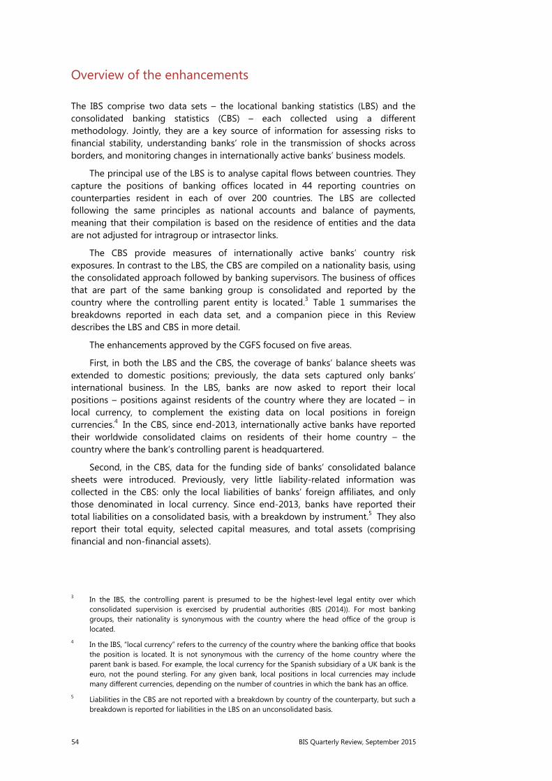
54 BIS Quarterly Review, September 2015
Overview of the enhancements
The IBS comprise two data sets – the locational banking statistics (LBS) and the consolidated banking statistics (CBS) – each collected using a different methodology. Jointly, they are a key source of information for assessing risks to financial stability, understanding banks’ role in the transmission of shocks across borders, and monitoring changes in internationally active banks’ business models.
The principal use of the LBS is to analyse capital flows between countries. They capture the positions of banking offices located in 44 reporting countries on counterparties resident in each of over 200 countries. The LBS are collected following the same principles as national accounts and balance of payments, meaning that their compilation is based on the residence of entities and the data are not adjusted for intragroup or intrasector links.
The CBS provide measures of internationally active banks’ country risk exposures. In contrast to the LBS, the CBS are compiled on a nationality basis, using the consolidated approach followed by banking supervisors. The business of offices that are part of the same banking group is consolidated and reported by the country where the controlling parent entity is located.3 Table 1 summarises the breakdowns reported in each data set, and a companion piece in this Review describes the LBS and CBS in more detail.
The enhancements approved by the CGFS focused on five areas.
First, in both the LBS and the CBS, the coverage of banks’ balance sheets was extended to domestic positions; previously, the data sets captured only banks’ international business. In the LBS, banks are now asked to report their local positions – positions against residents of the country where they are located – in local currency, to complement the existing data on local positions in foreign currencies.4 In the CBS, since end-2013, internationally active banks have reported their worldwide consolidated claims on residents of their home country – the country where the bank’s controlling parent is headquartered.
Second, in the CBS, data for the funding side of banks’ consolidated balance sheets were introduced. Previously, very little liability-related information was collected in the CBS: only the local liabilities of banks’ foreign affiliates, and only those denominated in local currency. Since end-2013, banks have reported their total liabilities on a consolidated basis, with a breakdown by instrument.5 They also report their total equity, selected capital measures, and total assets (comprising financial and non-financial assets).
3 In the IBS, the controlling parent is presumed to be the highest-level legal entity over which consolidated supervision is exercised by prudential authorities (BIS (2014)). For most banking groups, their nationality is synonymous with the country where the head office of the group is located.
4 In the IBS, “local currency” refers to the currency of the country where the banking office that books the position is located. It is not synonymous with the currency of the home country where the parent bank is based. For example, the local currency for the Spanish subsidiary of a UK bank is the euro, not the pound sterling. For any given bank, local positions in local currencies may include many different currencies, depending on the number of countries in which the bank has an office.
5 Liabilities in the CBS are not reported with a breakdown by country of the counterparty, but such a breakdown is reported for liabilities in the LBS on an unconsolidated basis.
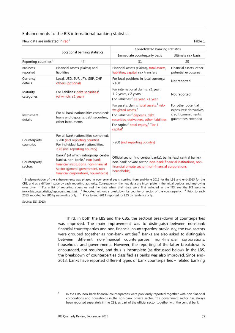
BIS Quarterly Review, September 2015 55
Third, in both the LBS and the CBS, the sectoral breakdown of counterparties was improved. The main improvement was to distinguish between non-bank financial counterparties and non-financial counterparties; previously, the two sectors were grouped together as non-bank entities.6 Banks are also asked to distinguish between different non-financial counterparties: non-financial corporations, households and governments. However, the reporting of the latter breakdown is encouraged, not required, and thus is incomplete (as discussed below). In the LBS, the breakdown of counterparties classified as banks was also improved. Since end-2013, banks have reported different types of bank counterparties – related banking
6 In the CBS, non-bank financial counterparties were previously reported together with non-financial corporations and households in the non-bank private sector. The government sector has always been reported separately in the CBS, as part of the official sector together with the central bank.
Enhancements to the BIS international banking statistics
New data are indicated in red1 Table 1
Locational banking statistics Consolidated banking statistics
Immediate counterparty basis Ultimate risk basis
Reporting countries2 44 31 25
Business reported
Financial assets (claims) and liabilities
Financial assets (claims), total assets, liabilities, capital, risk transfers
Financial assets, other potential exposures
Currency details
Local, USD, EUR, JPY, GBP, CHF, others (optional)
For local positions in local currency: >160
Not reported
Maturity categories
For liabilities: debt securities3 (of which: ≤1 year)
For international claims: ≤1 year, 1–2 years, >2 years. For liabilities:3 ≤1 year, >1 year
Not reported
Instrument details
For all bank nationalities combined: loans and deposits, debt securities, other instruments
For assets: claims, total assets,3 risk-weighted assets.3 For liabilities:3 deposits, debt securities, derivatives, other liabilities. For capital:3 total equity,3 Tier 1 capital3
For other potential exposures: derivatives, credit commitments, guarantees extended
Counterparty countries
For all bank nationalities combined: >200 (incl reporting country). For individual bank nationalities: ≥76 (incl reporting country)
>200 (incl reporting country)
Counterparty sectors
Banks4 (of which: intragroup, central banks), non-banks,5 non-bank financial institutions, non-financial sector (general government, non-financial corporations, households)
Official sector (incl central banks), banks (excl central banks), non-bank private sector, non-bank financial institutions, non-financial private sector (non-financial corporations, households)
1 Implementation of the enhancements was phased in over several years, starting from end-June 2012 for the LBS and end-2013 for the CBS, and at a different pace by each reporting authority. Consequently, the new data are incomplete in the initial periods and improving over time. 2 For a list of reporting countries and the date when their data were first included in the IBS, see the BIS website(www.bis.org/statistics/rep_countries.htm). 3 Reported without a breakdown by country or sector of the counterparty. 4 Prior to end-2013, reported for LBS by nationality only. 5 Prior to end-2013, reported for LBS by residence only.
Source: BIS (2013).
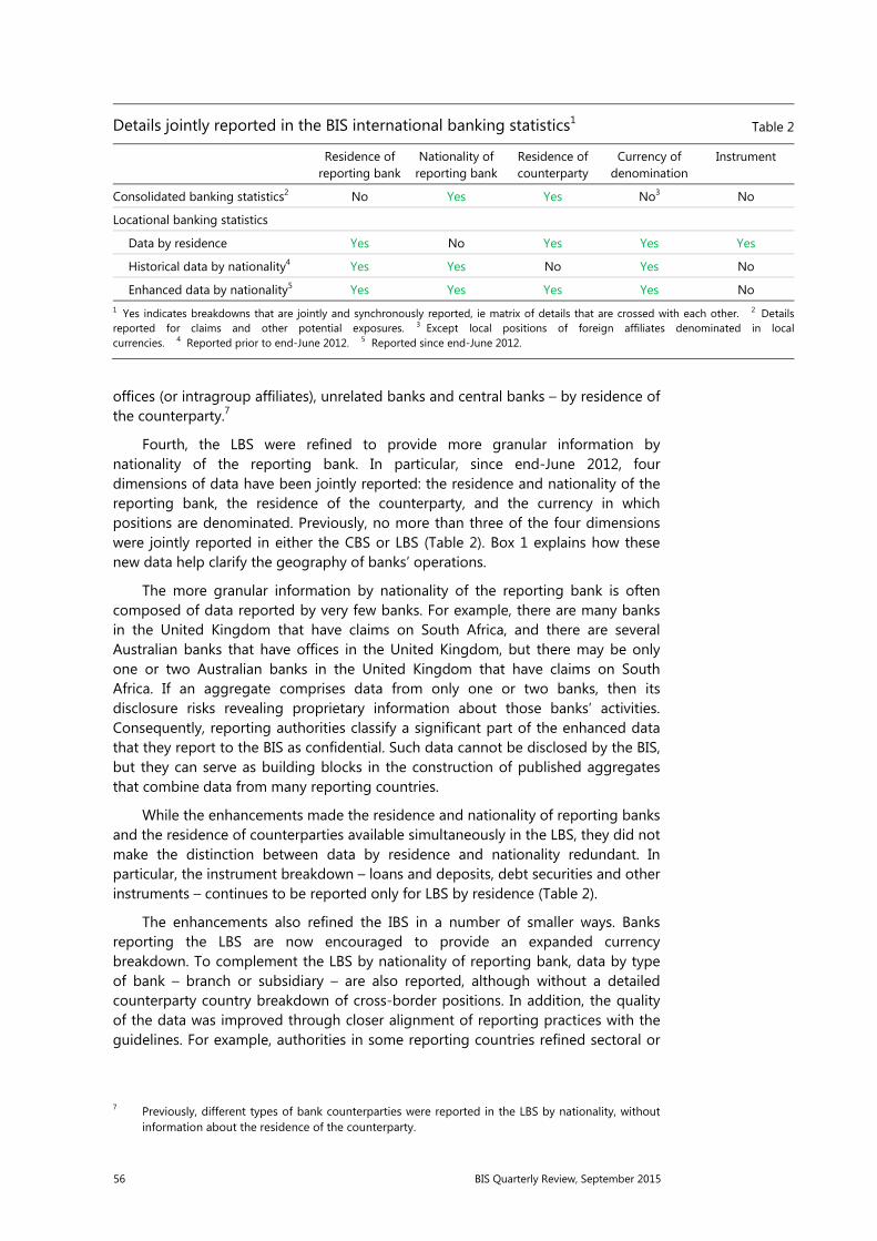
56 BIS Quarterly Review, September 2015
offices (or intragroup affiliates), unrelated banks and central banks – by residence of the counterparty.7
Fourth, the LBS were refined to provide more granular information by nationality of the reporting bank. In particular, since end-June 2012, four dimensions of data have been jointly reported: the residence and nationality of the reporting bank, the residence of the counterparty, and the currency in which positions are denominated. Previously, no more than three of the four dimensions were jointly reported in either the CBS or LBS (Table 2). Box 1 explains how these new data help clarify the geography of banks’ operations.
The more granular information by nationality of the reporting bank is often composed of data reported by very few banks. For example, there are many banks in the United Kingdom that have claims on South Africa, and there are several Australian banks that have offices in the United Kingdom, but there may be only one or two Australian banks in the United Kingdom that have claims on South Africa. If an aggregate comprises data from only one or two banks, then its disclosure risks revealing proprietary information about those banks’ activities. Consequently, reporting authorities classify a significant part of the enhanced data that they report to the BIS as confidential. Such data cannot be disclosed by the BIS, but they can serve as building blocks in the construction of published aggregates that combine data from many reporting countries.
While the enhancements made the residence and nationality of reporting banks and the residence of counterparties available simultaneously in the LBS, they did not make the distinction between data by residence and nationality redundant. In particular, the instrument breakdown – loans and deposits, debt securities and other instruments – continues to be reported only for LBS by residence (Table 2).
The enhancements also refined the IBS in a number of smaller ways. Banks reporting the LBS are now encouraged to provide an expanded currency breakdown. To complement the LBS by nationality of reporting bank, data by type of bank – branch or subsidiary – are also reported, although without a detailed counterparty country breakdown of cross-border positions. In addition, the quality of the data was improved through closer alignment of reporting practices with the guidelines. For example, authorities in some reporting countries refined sectoral or
7 Previously, different types of bank counterparties were reported in the LBS by nationality, without information about the residence of the counterparty.
Details jointly reported in the BIS international banking statistics1 Table 2
Residence ofreporting bank
Nationality ofreporting bank
Residence ofcounterparty
Currency of denomination
Instrument
Consolidated banking statistics2 No Yes Yes No3 No
Locational banking statistics
Data by residence Yes No Yes Yes Yes
Historical data by nationality4 Yes Yes No Yes No
Enhanced data by nationality5 Yes Yes Yes Yes No 1 Yes indicates breakdowns that are jointly and synchronously reported, ie matrix of details that are crossed with each other. 2 Details reported for claims and other potential exposures. 3 Except local positions of foreign affiliates denominated in local currencies. 4 Reported prior to end-June 2012. 5 Reported since end-June 2012.
BIS Quarterly Review, September 2015 57
other classifications. Such methodological changes have sometimes led to significant changes in reported outstanding positions.
Finally, the BIS comprehensively revised the tables presenting the IBS so as to include data collected as part of the enhancements (Box 2). The enhancements also prompted the BIS to revisit the way in which some aggregates are calculated or presented, resulting in changes to previously published data (Box 3).
Putting banks’ international business in context
The enhanced IBS provide a more comprehensive picture of the size and scope of internationally active banks’ activities. This enables better analysis of the sources and uses of funds and the importance of international business for banks of different nationalities.
The new data on domestic positions can be used to understand the relative importance of internationally active banks in the provision of total bank credit to borrowers in a particular economy. Previously, such analysis was limited to selected components of bank credit. Table 3 illustrates the enhanced LBS using data
Canadian banks’ worldwide claims and all banks’ claims on Canada
Amounts outstanding at end-March 2015, in billions of US dollars Table 3
Locational banking statistics
Consolidated banking statistics1
All LBS- reporting banks
Canadian banks Canadian banks on all
sectors of which:
intragroup
Claims on all countries 89,915 2,845 494 2,998
Claims on residents of Canada 2,366 1,959 107 1,787
Local claims of offices in Canada2 1,908 1,772 … …
in local currency3 (CAD) 1,825 1,711 … 1,700
in foreign currencies 83 61 … 6 87
Cross-border claims 457 187 107
in CAD4 1 – – …
in other currencies5 456 187 107 …
Claims on the rest of the world 87,549 886 388 1,211
Local claims2 59,613 152 23 …
in local currencies3 55,393 90 7 775
in foreign currencies 4,125 63 16 6 436
Cross-border claims 27,583 728 364 1 Claims on an immediate counterparty basis. 2 Claims booked by banking offices located in the same country as thecounterparty. 3 Claims denominated in the currency of the country where the banking office is located. 4 Data on cross-border claims denominated in Canadian dollars (CAD) are incomplete. 5 Other currencies may include CAD where not reported separately. 6 Cross-border claims in all currencies and local claims in foreign currencies are reported together as international claims.
Sources: BIS consolidated banking statistics (Tables B2 and B4.5); BIS locational banking statistics (Tables A5.8, A6.6 and A7.1).
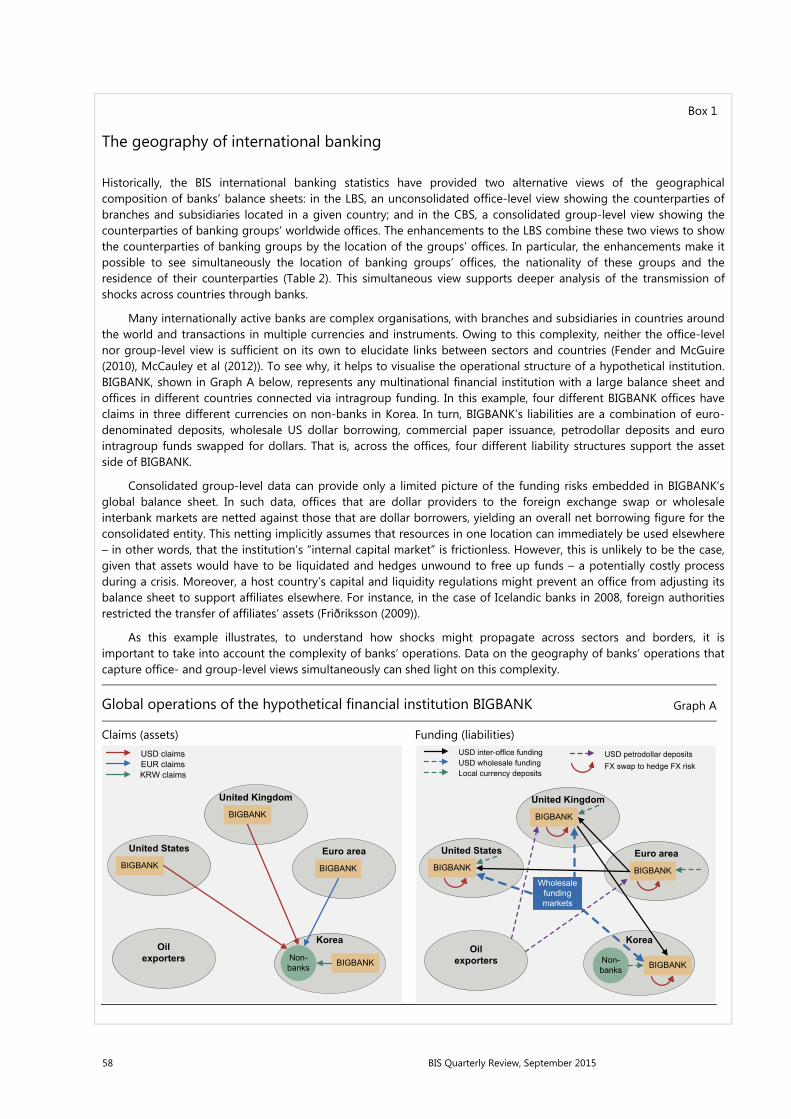
58 BIS Quarterly Review, September 2015
Box 1
The geography of international banking
Historically, the BIS international banking statistics have provided two alternative views of the geographical composition of banks’ balance sheets: in the LBS, an unconsolidated office-level view showing the counterparties of branches and subsidiaries located in a given country; and in the CBS, a consolidated group-level view showing the counterparties of banking groups’ worldwide offices. The enhancements to the LBS combine these two views to show the counterparties of banking groups by the location of the groups’ offices. In particular, the enhancements make it possible to see simultaneously the location of banking groups’ offices, the nationality of these groups and the residence of their counterparties (Table 2). This simultaneous view supports deeper analysis of the transmission of shocks across countries through banks.
Many internationally active banks are complex organisations, with branches and subsidiaries in countries around the world and transactions in multiple currencies and instruments. Owing to this complexity, neither the office-level nor group-level view is sufficient on its own to elucidate links between sectors and countries (Fender and McGuire (2010), McCauley et al (2012)). To see why, it helps to visualise the operational structure of a hypothetical institution. BIGBANK, shown in Graph A below, represents any multinational financial institution with a large balance sheet and offices in different countries connected via intragroup funding. In this example, four different BIGBANK offices have claims in three different currencies on non-banks in Korea. In turn, BIGBANK’s liabilities are a combination of euro-denominated deposits, wholesale US dollar borrowing, commercial paper issuance, petrodollar deposits and euro intragroup funds swapped for dollars. That is, across the offices, four different liability structures support the asset side of BIGBANK.
Consolidated group-level data can provide only a limited picture of the funding risks embedded in BIGBANK’s global balance sheet. In such data, offices that are dollar providers to the foreign exchange swap or wholesale interbank markets are netted against those that are dollar borrowers, yielding an overall net borrowing figure for the consolidated entity. This netting implicitly assumes that resources in one location can immediately be used elsewhere – in other words, that the institution’s “internal capital market” is frictionless. However, this is unlikely to be the case,given that assets would have to be liquidated and hedges unwound to free up funds – a potentially costly process during a crisis. Moreover, a host country’s capital and liquidity regulations might prevent an office from adjusting its balance sheet to support affiliates elsewhere. For instance, in the case of Icelandic banks in 2008, foreign authorities restricted the transfer of affiliates’ assets (Friðriksson (2009)).
As this example illustrates, to understand how shocks might propagate across sectors and borders, it is important to take into account the complexity of banks’ operations. Data on the geography of banks’ operations that capture office- and group-level views simultaneously can shed light on this complexity.
Global operations of the hypothetical financial institution BIGBANK Graph A
Claims (assets) Funding (liabilities)
Korea
BIGBANKNon-banks
United StatesBIGBANK
United KingdomBIGBANK
Euro areaBIGBANK
Oil exporters
KRW claimsEUR claimsUSD claims
Korea
BIGBANKNon-banks
United StatesBIGBANK
United KingdomBIGBANK
Euro areaBIGBANK
Oil exporters
FX swap to hedge FX riskLocal currency depositsUSD wholesale fundingUSD inter-office funding USD petrodollar deposits
Wholesale funding markets
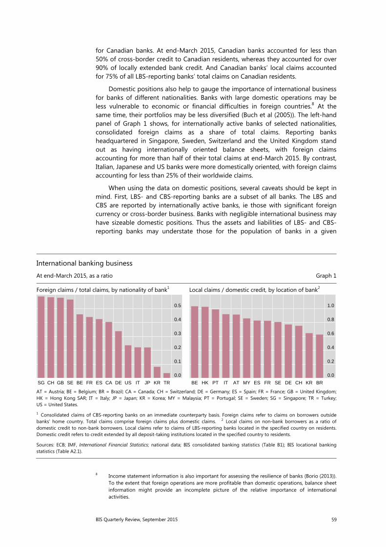
BIS Quarterly Review, September 2015 59
for Canadian banks. At end-March 2015, Canadian banks accounted for less than 50% of cross-border credit to Canadian residents, whereas they accounted for over 90% of locally extended bank credit. And Canadian banks’ local claims accounted for 75% of all LBS-reporting banks’ total claims on Canadian residents.
Domestic positions also help to gauge the importance of international business for banks of different nationalities. Banks with large domestic operations may be less vulnerable to economic or financial difficulties in foreign countries.8 At the same time, their portfolios may be less diversified (Buch et al (2005)). The left-hand panel of Graph 1 shows, for internationally active banks of selected nationalities, consolidated foreign claims as a share of total claims. Reporting banks headquartered in Singapore, Sweden, Switzerland and the United Kingdom stand out as having internationally oriented balance sheets, with foreign claims accounting for more than half of their total claims at end-March 2015. By contrast, Italian, Japanese and US banks were more domestically oriented, with foreign claims accounting for less than 25% of their worldwide claims.
When using the data on domestic positions, several caveats should be kept in mind. First, LBS- and CBS-reporting banks are a subset of all banks. The LBS and CBS are reported by internationally active banks, ie those with significant foreign currency or cross-border business. Banks with negligible international business may have sizeable domestic positions. Thus the assets and liabilities of LBS- and CBS-reporting banks may understate those for the population of banks in a given
8 Income statement information is also important for assessing the resilience of banks (Borio (2013)). To the extent that foreign operations are more profitable than domestic operations, balance sheet information might provide an incomplete picture of the relative importance of international activities.
International banking business
At end-March 2015, as a ratio Graph 1
Foreign claims / total claims, by nationality of bank1 Local claims / domestic credit, by location of bank2
AT = Austria; BE = Belgium; BR = Brazil; CA = Canada; CH = Switzerland; DE = Germany; ES = Spain; FR = France; GB = United Kingdom; HK = Hong Kong SAR; IT = Italy; JP = Japan; KR = Korea; MY = Malaysia; PT = Portugal; SE = Sweden; SG = Singapore; TR = Turkey; US = United States.
1 Consolidated claims of CBS-reporting banks on an immediate counterparty basis. Foreign claims refer to claims on borrowers outsidebanks’ home country. Total claims comprise foreign claims plus domestic claims. 2 Local claims on non-bank borrowers as a ratio of domestic credit to non-bank borrowers. Local claims refer to claims of LBS-reporting banks located in the specified country on residents. Domestic credit refers to credit extended by all deposit-taking institutions located in the specified country to residents.
Sources: ECB; IMF, International Financial Statistics; national data; BIS consolidated banking statistics (Table B1); BIS locational bankingstatistics (Table A2.1).
0.0
0.1
0.2
0.3
0.4
0.5
SG CH GB SE BE FR ES CA DE US IT JP KR TR
0.0
0.2
0.4
0.6
0.8
1.0
BE HK PT IT AT MY ES FR SE DE CH KR BR

60 BIS Quarterly Review, September 2015
Box 2
New tables on the international banking statistics
The BIS comprehensively revised the tables on the international banking statistics. The new tables include more data, notably new data collected as part of the enhancements to the locational banking statistics (LBS) and the consolidated banking statistics (CBS), and present these data in a more user-friendly way. In particular, the BIS introduced country tables that bring together in one table data for banks’ positions on a given country that were previously spread across several tables.
The new tables on the LBS are published in Section A of the BIS Statistical Bulletin, and those on the CBS in Section B. Each section starts with global tables that summarise the data, followed by country tables with more details. While the country tables in the PDF version of the Bulletin show only selected countries, tables covering additional countries are available on the BIS website (www.bis.org/statistics/bankstats.htm) or in the new BIS Statistics Explorer (stats.bis.org/statx/).
Tables A1 to A4 provide an overview of the LBS disaggregated by sector of the counterparty. Table A1 summarises the different breakdowns available: in addition to sector, it presents data by region where the counterparty resides, currency and instrument. Table A2 shows the sectoral composition of LBS-reporting banks’ claims and liabilities by location of the bank, ie positions of banks in a given reporting country on all counterparties abroad. Table A3 shows the sectoral composition of claims and liabilities on counterparties in over 200 individual countries, ie cross-border positions of all LBS-reporting banks on counterparties in a given country. Table A4 shows the sectoral composition of cross-border positions for banks of a given nationality. For each table, data on amounts outstanding and break- and exchange rate-adjusted changes are published.
Country tables A5 to A7 present detailed views of the LBS from three different perspectives: location of the reporting bank, residence of the counterparty, and nationality of the reporting bank, respectively. The BIS plans to publish additional data in these tables in the future as their quality and completeness improve. Table A8 presents LBS-reporting banks’ claims and liabilities on the central bank sector.
Tables B1 to B3 provide an overview of the CBS reported by banks of different nationalities, albeit without any details by country of the counterparty. Table B1 summarises the total claims of CBS-reporting banks, distinguishing between domestic and foreign claims. Table B1 also presents their total assets/liabilities by instrument and equity. Table B2 shows foreign claims on an immediate counterparty basis, including a breakdown of the international component of claims by sector and remaining maturity. Table B3 presents foreign claims and other potential foreign exposures on an ultimate risk basis.
Country table B4 presents bilateral CBS for banks of different nationalities on counterparties in a given country. While the Bulletin shows data for 29 countries, data for over 200 countries are available on the BIS website. Table B4 distinguishes between foreign banks and domestic banks. The term “foreign banks” refers to banks headquartered abroad (or, more precisely, controlled by parents abroad). These are mostly banks from CBS-reporting countries, but include the unconsolidated positions of banking offices located in CBS-reporting countries and headquartered elsewhere. Domestic banks are those headquartered in the country. For example, in the table for Japan, the claims of Japanese banks on residents of Japan are shown under domestic banks, in the row labelled “Worldwide offices (consolidated)”. Under foreign banks, the row for Japan is blank.
The tables in Section A replace Tables 1–8 of the former Statistical Annex, and those in Section B replace Tables 9A–9E. An explanationof where to find data from the old tables in the new tables is available on the BIS website (www.bis.org/statistics/annex_map.htm).
country or of a given nationality. Also, definitions and balance sheet coverage in the IBS might differ from those applied in other data sets, such as national monetary and financial statistics (MFS).
The right-hand panel of Graph 1 compares the local claims of LBS-reporting banks on non-bank borrowers in a given country with domestic bank credit from MFS. For most countries, the ratio is below but close to one. In a few cases, such as Japan, the ratio exceeds one because the LBS include some assets not included in

BIS Quarterly Review, September 2015 61
the MFS. In other cases, such as Brazil and Korea, the ratio is much less than one because the LBS exclude the assets of large domestic banks with little international business.
Furthermore, even though more countries report the LBS than do the CBS, the global coverage of the LBS is less complete than that of the CBS. The CBS are collected on a consolidated basis and so capture the positions of banks’ affiliates worldwide. By contrast, the LBS capture only the positions of affiliates in LBS-reporting countries. To the extent that a given banking system has large operations in non-reporting countries, or in reporting countries that do not report all of the requested data, the LBS by nationality of the reporting bank can misrepresent the global activities of the relevant banking system. For example, Canadian banks’ consolidated claims on all countries totalled $3.0 trillion at end-March 2015 (Table 3). Of this amount, only $2.4 trillion was captured in the LBS (after subtracting intragroup positions). The main reason for the gap is that local positions booked by Canadian banks’ offices in the United States and some Caribbean countries are not included in the LBS because these countries have not yet reported the requested data. In addition, the CBS may include the claims of reporting banks’ non-bank subsidiaries that are within their supervisory or accounting perimeter (eg securities dealers), whereas the LBS exclude the claims of such entities.
Understanding banks’ counterparties
The IBS have long provided detailed information about the countries where banks’ counterparties reside but limited information about the sectors in which these counterparties are active. The enhancements support a more detailed analysis of the build-up of risks in particular sectors, especially within the non-bank private sector, which comprises non-bank financial institutions, non-financial corporations and households.
The Great Financial Crisis revealed the shortcomings of focusing on countries and neglecting sectors. Even when vulnerabilities are not apparent in a given economy, weaknesses in particular sectors can be transmitted globally through cross-border bank exposures and have wider consequences for financial stability. For instance, in the 2000s, some foreign banks built up large exposures to the US household sector, which subsequently exacerbated spillovers from the subprime mortgage crisis. Banks’ exposures to special purpose vehicles, securities brokers, hedge funds and other non-bank financial entities – the so-called “shadow banking” system – also built up significantly over this period.9
The enhancements shed light on exposures to the non-bank private sector. Table 4 shows the sectoral composition of LBS reporting banks’ cross-border claims on selected regions. Banks in some reporting countries have not yet reported the new sectors, and thus the allocated share of positions is relatively low, less than 75% overall. For this reason, the new tables published in the BIS Statistical Bulletin do not yet show the new sectors for individual counterparty countries; the data will be added once these breakdowns are more widely reported.
9 The shadow banking system can broadly be described as credit intermediation involving entities and activities outside the regular banking system (FSB (2014)).
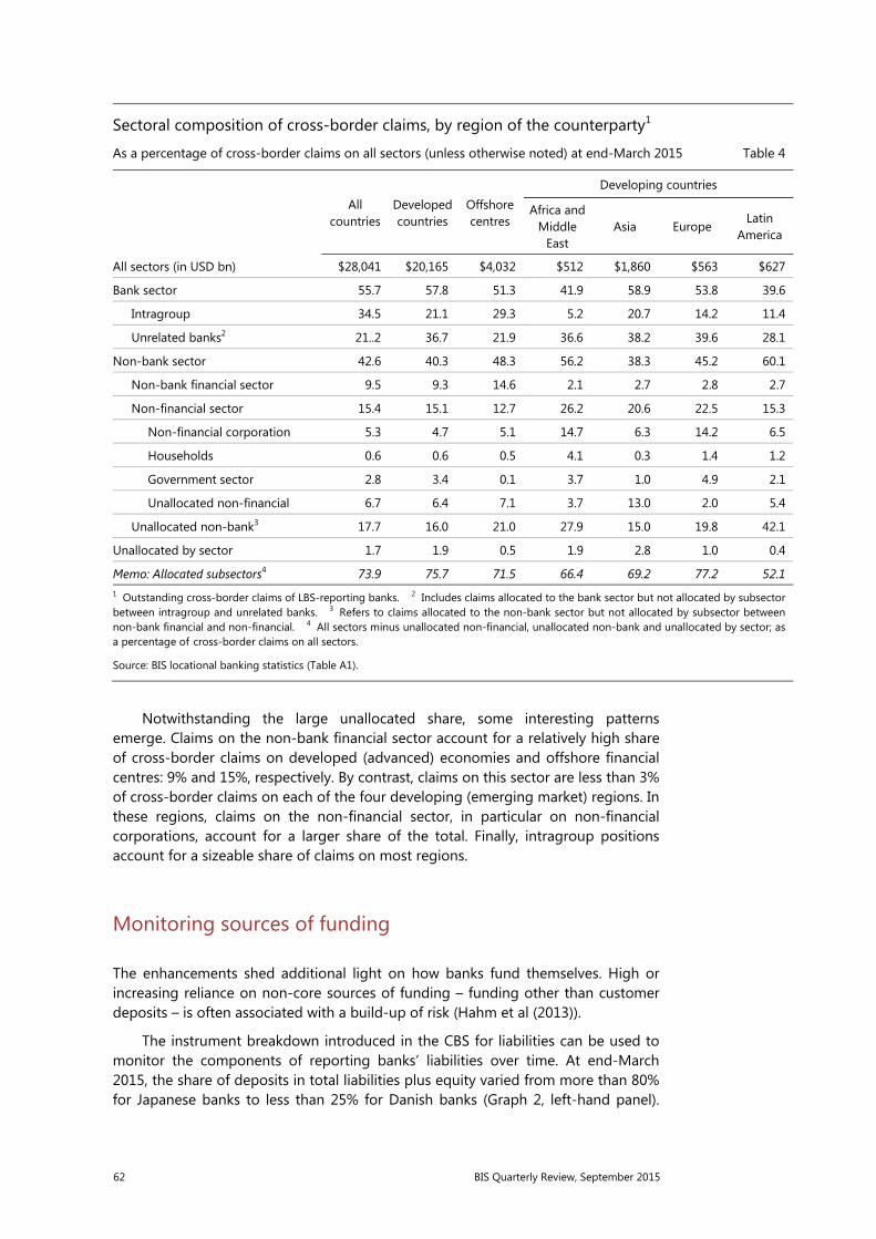
62 BIS Quarterly Review, September 2015
Notwithstanding the large unallocated share, some interesting patterns emerge. Claims on the non-bank financial sector account for a relatively high share of cross-border claims on developed (advanced) economies and offshore financial centres: 9% and 15%, respectively. By contrast, claims on this sector are less than 3% of cross-border claims on each of the four developing (emerging market) regions. In these regions, claims on the non-financial sector, in particular on non-financial corporations, account for a larger share of the total. Finally, intragroup positions account for a sizeable share of claims on most regions.
Monitoring sources of funding
The enhancements shed additional light on how banks fund themselves. High or increasing reliance on non-core sources of funding – funding other than customer deposits – is often associated with a build-up of risk (Hahm et al (2013)).
The instrument breakdown introduced in the CBS for liabilities can be used to monitor the components of reporting banks’ liabilities over time. At end-March 2015, the share of deposits in total liabilities plus equity varied from more than 80% for Japanese banks to less than 25% for Danish banks (Graph 2, left-hand panel).
Sectoral composition of cross-border claims, by region of the counterparty1
As a percentage of cross-border claims on all sectors (unless otherwise noted) at end-March 2015 Table 4
All countries
Developedcountries
Offshorecentres
Developing countries
Africa and Middle
East Asia Europe
Latin America
All sectors (in USD bn) $28,041 $20,165 $4,032 $512 $1,860 $563 $627
Bank sector 55.7 57.8 51.3 41.9 58.9 53.8 39.6
Intragroup 34.5 21.1 29.3 5.2 20.7 14.2 11.4
Unrelated banks2 21..2 36.7 21.9 36.6 38.2 39.6 28.1
Non-bank sector 42.6 40.3 48.3 56.2 38.3 45.2 60.1
Non-bank financial sector 9.5 9.3 14.6 2.1 2.7 2.8 2.7
Non-financial sector 15.4 15.1 12.7 26.2 20.6 22.5 15.3
Non-financial corporation 5.3 4.7 5.1 14.7 6.3 14.2 6.5
Households 0.6 0.6 0.5 4.1 0.3 1.4 1.2
Government sector 2.8 3.4 0.1 3.7 1.0 4.9 2.1
Unallocated non-financial 6.7 6.4 7.1 3.7 13.0 2.0 5.4
Unallocated non-bank3 17.7 16.0 21.0 27.9 15.0 19.8 42.1
Unallocated by sector 1.7 1.9 0.5 1.9 2.8 1.0 0.4
Memo: Allocated subsectors4 73.9 75.7 71.5 66.4 69.2 77.2 52.1 1 Outstanding cross-border claims of LBS-reporting banks. 2 Includes claims allocated to the bank sector but not allocated by subsector between intragroup and unrelated banks. 3 Refers to claims allocated to the non-bank sector but not allocated by subsector between non-bank financial and non-financial. 4 All sectors minus unallocated non-financial, unallocated non-bank and unallocated by sector; as a percentage of cross-border claims on all sectors.
Source: BIS locational banking statistics (Table A1).
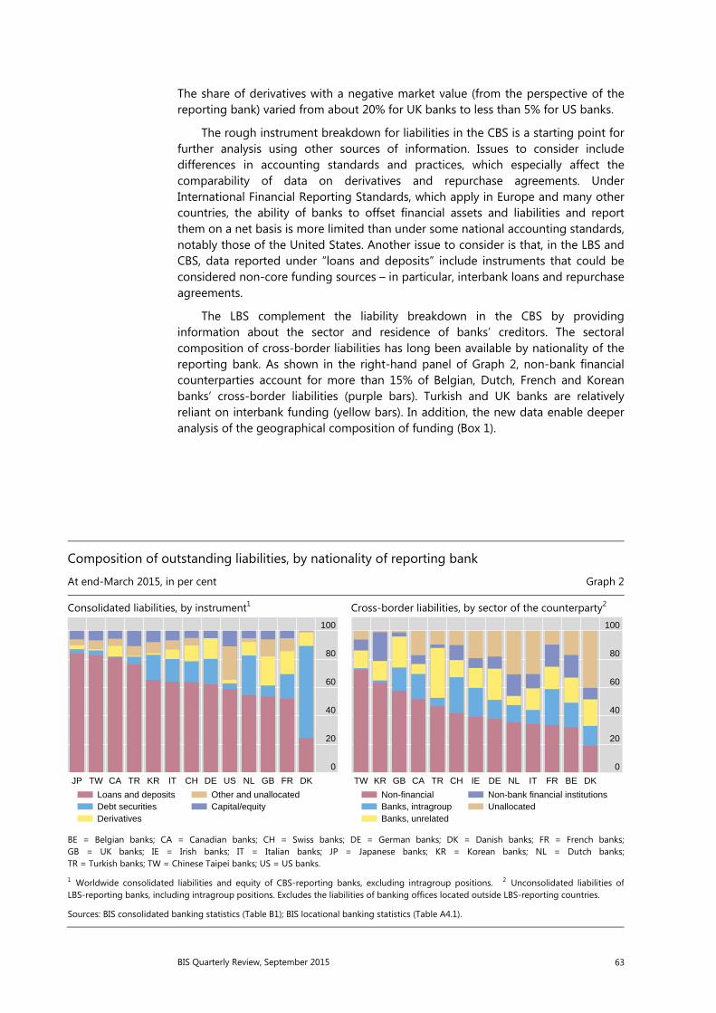
BIS Quarterly Review, September 2015 63
The share of derivatives with a negative market value (from the perspective of the reporting bank) varied from about 20% for UK banks to less than 5% for US banks.
The rough instrument breakdown for liabilities in the CBS is a starting point for further analysis using other sources of information. Issues to consider include differences in accounting standards and practices, which especially affect the comparability of data on derivatives and repurchase agreements. Under International Financial Reporting Standards, which apply in Europe and many other countries, the ability of banks to offset financial assets and liabilities and report them on a net basis is more limited than under some national accounting standards, notably those of the United States. Another issue to consider is that, in the LBS and CBS, data reported under “loans and deposits” include instruments that could be considered non-core funding sources – in particular, interbank loans and repurchase agreements.
The LBS complement the liability breakdown in the CBS by providing information about the sector and residence of banks’ creditors. The sectoral composition of cross-border liabilities has long been available by nationality of the reporting bank. As shown in the right-hand panel of Graph 2, non-bank financial counterparties account for more than 15% of Belgian, Dutch, French and Korean banks’ cross-border liabilities (purple bars). Turkish and UK banks are relatively reliant on interbank funding (yellow bars). In addition, the new data enable deeper analysis of the geographical composition of funding (Box 1).
Composition of outstanding liabilities, by nationality of reporting bank
At end-March 2015, in per cent Graph 2
Consolidated liabilities, by instrument1 Cross-border liabilities, by sector of the counterparty2
BE = Belgian banks; CA = Canadian banks; CH = Swiss banks; DE = German banks; DK = Danish banks; FR = French banks;GB = UK banks; IE = Irish banks; IT = Italian banks; JP = Japanese banks; KR = Korean banks; NL = Dutch banks;TR = Turkish banks; TW = Chinese Taipei banks; US = US banks.
1 Worldwide consolidated liabilities and equity of CBS-reporting banks, excluding intragroup positions. 2 Unconsolidated liabilities of LBS-reporting banks, including intragroup positions. Excludes the liabilities of banking offices located outside LBS-reporting countries.
Sources: BIS consolidated banking statistics (Table B1); BIS locational banking statistics (Table A4.1).
0
20
40
60
80
100
JP TW CA TR KR IT CH DE US NL GB FR DK
Loans and depositsDebt securitiesDerivatives
Other and unallocatedCapital/equity
0
20
40
60
80
100
TW KR GB CA TR CH IE DE NL IT FR BE DK
Non-financialBanks, intragroupBanks, unrelated
Non-bank financial institutionsUnallocated
64 BIS Quarterly Review, September 2015
Box 3
Revisions to historical LBS and CBS
In conjunction with the release of new data collected as part of the enhancements, the BIS has revised some data published previously in the LBS and CBS. These revisions take advantage of the new data to improve the quality of aggregates calculated by the BIS. However, they result in some discontinuities in historical data.
In the LBS, data for the bank sector were revised to exclude positions unallocated by counterparty sector. Previously, the BIS estimated positions vis-à-vis the bank sector in individual counterparty countries as all sectors minus the non-bank sector. Consequently, the bank sector included positions unallocated by counterparty sector. From end-June 2012, the BIS began to collect positions unallocated by sector separately as well as positions vis-à-vis bank subsectors allocated by counterparty country. These new data enabled estimates for the bank sector to be improved. While the full history of estimates has been revised, the impact is most noticeable starting from end-June 2012. The impact of the revisions to the bank sector is especially significant for interbank liabilities. As of end-2014, the exclusion of unallocated positions reduced BIS reporting banks’ outstanding cross-border liabilities to banking offices by $2.2 trillion to $15.2 trillion. By contrast, their exclusion reduced interbank claims by only $0.5 trillion to $16.2 trillion.
In the CBS, data for the positions of all reporting banks on counterparties in a given country were revised to distinguish more clearly between the positions of foreign and domestic banks, where domestic banks are those headquartered in the respective country. Historically, some data reported by domestic banks were mixed with data from foreign banks in the case of counterparty countries that were also CBS-reporting countries. In particular, claims of all reporting banks on an immediate counterparty basis included the unconsolidated cross-border claims of domestic banks’ foreign offices on residents of the banks’ home country. For example, claims on Japan previously included the claims of Japanese banks’ offices in other CBS-reporting countries. As of end-March 2015, the unconsolidated claims of Japanese banks’ foreign offices on Japan totalled $0.5 trillion. The claims of foreign (non-Japanese) banks on Japan totalled $0.8 trillion on an immediate counterparty basis. Whereas these two figures were previously added together in the data published by the BIS for all reporting banks (in what used to be Table 9A), data for domestic and foreign banks are now shown separately (in the new Table B4).
From end-2013, the BIS began to collect domestic positions on a consolidated basis: the worldwide positions of banking groups on residents of the groups’ home country. These data are more comprehensive than the data reported by domestic banks’ foreign offices. To facilitate historical comparisons, in Table B4 the BIS publishes consolidated data for the worldwide offices of domestic banks as well as the unconsolidated data of their foreign offices. Data for domestic banks are available only for counterparty countries that are also CBS-reporting countries (and some of these do not yet report domestic positions).
Finally, the BIS revised the labels of some data to clarify what they covered. In the CBS, data on an immediate borrower basis were renamed data on an immediate counterparty basis, in recognition of the fact that the data now cover liabilities as well as assets. Also, the public sector was renamed the official sector to clarify that it refers only to positions on the government sector and central bank and does not include positions on publicly owned corporations.
Prior to end-June 2012, the BIS collected data for the bank sector and subsectors without a breakdown by counterparty country;historically, the LBS by individual counterparty country were collected only for all sectors and for the non-bank sector. Prior to end-June 2012, data unallocated by sector are incomplete. This is one of two pieces of unconsolidated data that have historically been included in the total for all reporting banks, the other piece being the unconsolidated cross-border claims of banking offices with parent banks headquartered outside the BIS reporting area. The BIS continues to include the latter piece in the total for foreign banks. Whereas domestic positions are reported by the home country and capture worldwide consolidated positions, data on foreign offices’ claims on residents of the home country are reported by countries where the office is located and hence omit the claims of offices located outside the CBS-reporting countries.
Along with the caveats discussed above regarding data on domestic positions, use of the LBS to analyse the composition of liabilities needs to take account of liabilities that banks are unable to allocate by counterparty. Whereas banks should always know the counterparty to whom they lend, they do not necessarily know the counterparty from whom they borrow, particularly when that borrowing takes the
BIS Quarterly Review, September 2015 65
form of negotiable instruments such as debt securities. Consequently, liabilities unallocated by counterparty can be large. Cross-border liabilities unallocated by sector of the counterparty equalled $2.2 trillion at end-March 2015, or 9% of outstanding cross-border liabilities.10 Banks’ own issues of debt securities accounted for nearly 80% of these liabilities.
Dissecting the currency composition
A unique feature of the LBS is their currency breakdown. The enhancements refine this breakdown and thereby facilitate a more accurate adjustment of quarterly changes in banks’ positions for exchange rate movements, as well as a fuller analysis of banks’ sources and uses of particular currencies.
One use of the enhanced currency breakdown is to improve estimates of underlying flows between quarters. In the IBS, only amounts outstanding are collected; flows are approximated by calculating changes in amounts outstanding adjusted for discontinuities in the data and exchange rate movements. Even in the absence of any flows, discontinuities can be introduced by changes in methodology, reporting practices or reporting population – so-called “breaks” in time series. Also, movements in exchange rates affect the US dollar value of amounts denominated in non-dollar currencies.11 Any additional information about breaks and the currency composition of positions therefore enables the BIS to improve its calculation of break- and exchange rate-adjusted changes.12
Furthermore, the currency breakdown, coupled with the new more granular counterparty data in the LBS by nationality of the reporting bank, enables the calculation of exchange rate-adjusted changes in claims for banks of a given nationality on residents of a given country. While such bilateral information has historically been available in the CBS for amounts outstanding, the calculation of exchange rate-adjusted changes for bank nationality-counterparty country pairs was not possible because the CBS do not have a comprehensive currency breakdown. Utilising the bilateral exchange rate-adjusted changes in claims derived from the enhanced LBS, Avdjiev and Takáts (2014) identify the demand and supply side drivers of the slowdown in cross-border bank lending to emerging market economies (EMEs) during the “taper tantrum” episode of 2013.
Another use of the currency breakdown is to analyse imbalances in funding markets. During the 2000s, many banks followed similar funding strategies. This funding equivalent of a “crowded trade” created systemic risks that aggravated the Great Financial Crisis (McGuire and von Peter (2012)). The new data provide better insights into the degree to which banks of different nationalities invest in one currency and fund in another. However, it should be kept in mind that, while such
10 Liabilities unallocated by either sector or residence of the counterparty amounted to a further $2.6 trillion at end-March 2013.
11 Amounts outstanding are reported to the BIS in US dollars. The depreciation of a given currency against the US dollar will result in a decline in the reported US dollar value of positions denominated in that currency, and an appreciation an increase.
12 Adjusted changes may still over- or underestimate underlying flows because of fluctuations in valuations, writedowns, the underreporting of breaks, and differences between the exchange rate on the transaction date and the quarterly average exchange rate used by the BIS to convert changes in non-dollar amounts into US dollars.
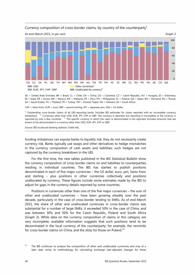
66 BIS Quarterly Review, September 2015
funding imbalances can expose banks to liquidity risk, they do not necessarily create currency risk. Banks typically use swaps and other derivatives to hedge mismatches in the currency composition of cash assets and liabilities; such hedges are not captured by the currency breakdown in the LBS.
For the first time, the new tables published in the BIS Statistical Bulletin show the currency composition of cross-border claims on and liabilities to counterparties residing in individual countries. The BIS has started to publish positions denominated in each of five major currencies – the US dollar, euro, yen, Swiss franc and sterling – plus positions in other currencies collectively and positions unallocated by currency. These figures include some estimates made by the BIS to adjust for gaps in the currency details reported by some countries.
Positions in currencies other than one of the five major currencies – the sum of other and unallocated currencies – have been growing steadily over the past decade, particularly in the case of cross-border lending to EMEs. As of end-March 2015, the share of other and unallocated currencies in cross-border claims was substantial for a number of large EMEs: it exceeded 50% in the case of China, and was between 30% and 50% for the Czech Republic, Poland and South Africa (Graph 3). While data on the currency composition of claims in this category are very incomplete, available information suggests that such positions tend to be denominated in the local currency of the counterparty: for example, the renminbi for cross-border claims on China, and the zloty for those on Poland.13
13 The BIS continues to analyse the composition of other and unallocated currencies and may at a later date revise its methodology for calculating exchange rate-adjusted changes for these
Currency composition of cross-border claims, by country of the counterparty1
At end-March 2015, in per cent Graph 3
AE = United Arab Emirates; BR = Brazil; CL = Chile; CN = China; CO = Colombia; CZ = Czech Republic; HU = Hungary; ID = Indonesia;IN = India; KR = Korea; MX = Mexico; MY = Malaysia; PE = Peru; PH = Philippines; PL = Poland; QA = Qatar; RO = Romania; RU = Russia; SA = Saudi Arabia; TH = Thailand; TR = Turkey; TW = Chinese Taipei; VN = Vietnam; ZA = South Africa.
CHF = Swiss franc; EUR = euro; GBP = pound sterling; JPY = Japanese yen; USD = US dollar.
1 Outstanding cross-border claims of all LBS-reporting banks. Includes BIS estimates for claims reported with an incomplete currency breakdown. 2 Currencies other than USD, EUR, JPY, CHF or GBP. The currency is reported, but reporting is incomplete, ie the currency isreported by only a few countries. 3 The specific currency in which the claim is denominated is not reported. Includes amounts that areknown to be denominated in a currency other than USD, EUR, JPY, CHF or GBP.
Source: BIS locational banking statistics (Table A6).
0
20
40
60
80
100
CN CZ ZA PL SA TH MY MX RO KR HU TW TR PH IN ID BR CL RU PE VN AE CO QA
USDEUR, JPY, CHF, GBP
Other currencies2
Unallocated by currency3
BIS Quarterly Review, September 2015 67
Completing the enhancements
The failure to anticipate the Great Financial Crisis can be attributed more to the faulty lens through which the existing statistics were examined than to a lack of adequate statistics (Borio (2013)). Nevertheless, the 2007–09 crisis, like many crises before it, highlighted the need for more detailed information. The enhancements to the BIS international banking statistics approved by the CGFS responded to this need and introduced new data to help analysts understand changes in the financial landscape and what consequences they might have for financial stability.
Although implementation of the enhancements began in 2012, it will be several more years before they are completed. In the near future, the global coverage of the IBS is expected to improve. Authorities in additional countries will be joining the reporting population. In particular, as part of the G20 Data Gaps Initiative, those G20 economies that do not yet participate in the IBS – Argentina, China, Russia and Saudi Arabia – are taking steps to join. In addition, the representativeness of aggregates comprising data from all reporting countries will improve as those reporting countries where implementation of the enhancements is currently lagging start to report the requested data.
The granularity of the enhanced data poses challenges (Avdjiev et al (2015)). First, the more granular the data, the greater are their volume and complexity, which in turn require adaptions of information systems by banks, reporting authorities and the BIS to maintain data quality. Second, as discussed above, more granular data are more likely to raise issues of confidentiality. Consolidation in the banking industry and the withdrawal of some banks from international banking activities since the Great Financial Crisis further increase this likelihood. Efforts are under way to address these challenges – for example, by constructing broad indicators that use granular data as building blocks, as well as encouraging individual banks to disclose more information about their international business.
The BIS plans to release additional data in the coming years as their completeness improves and the challenges posed by granularity are addressed. Indeed, one of the enhancements mandated by the CGFS was to make the IBS more widely available. The IBS are intended to help central banks, other policymakers and market participants analyse and manage risks, with greater transparency thereby contributing to financial stability. The new tables published in the BIS Statistical Bulletin are an important step on the road to this goal, and the BIS together with central banks will continue to work towards publishing more data and improving their accessibility.
positions. Currently, the BIS assumes that unallocated positions are denominated in the IMF’s Special Drawing Right (SDR), which is a basket composed of the US dollar, euro, yen and sterling, and adjusts outstanding positions using the SDR exchange rate against the US dollar.
68 BIS Quarterly Review, September 2015
References
Avdjiev, S, P McGuire and P Wooldridge (2015): “Enhancements to the BIS international banking statistics”, IFC Bulletin, no 39.
Avdjiev, S and E Takáts (2014): “Cross-border bank lending during the taper tantrum: the role of emerging market fundamentals”, BIS Quarterly Review, September, pp 49–60.
Bank for International Settlements (2011): “Closing data gaps to enhance systemic risk measurement”, 81st Annual Report, June, Chapter VI.
——— (2013): Guidelines for reporting the BIS international banking statistics: version incorporating Stage 1 and Stage 2 enhancements recommended by the CGFS, March.
——— (2014): “Guidelines for reporting the BIS international banking statistics: proposed revisions and clarifications to the March 2013 version”, July,
Borio, C (2013): “The great financial crisis: setting priorities for new statistics”, Journal of Banking Regulation, vol 14, pp 306–17 (also available as BIS Working Papers, no 408, April).
Buch, C, J Driscoll and C Ostergaard (2005): “Cross-border diversification in bank asset portfolios”, ECB Working Papers, no 429, January.
Committee on the Global Financial System (2009): “Credit risk transfer statistics”, CGFS Publications, no 35, September.
——— (2012): “Improving the BIS international banking statistics”, CGFS Publications, no 47, November.
Fender, I and P McGuire (2010): “Bank structure, funding risks and the transmission of shocks across countries: concepts and measurement”, BIS Quarterly Review, September, pp 63–79.
Financial Stability Board (2014): Global shadow banking monitoring report 2014, 30 October.
Financial Stability Board and International Monetary Fund (2009): “The financial crisis and information gaps”, report to the G20 Finance Ministers and Central Bank Governors, October.
Friðriksson, I (2009): “The banking crisis in Iceland in 2008”, remarks prepared for a seminar at the Bank of Finland, 6 February.
Hahm, J, H Song Shin and K Shin (2013): “Noncore bank liabilities and financial vulnerability”, Journal of Money, Credit and Banking, vol 45, August, pp 3–36.
McCauley, R, P McGuire and G von Peter (2012): “After the global financial crisis: from international to multinational banking?”, Journal of Economics and Business, vol 64, no 1, pp 7–23.
McGuire, P and G von Peter (2012): “The dollar shortage in global banking and the international policy response”, International Finance, vol 15, no 2, pp 155–78 (also available as BIS Working Papers, no 291, October 2009).
Vause, N (2011): “Enhanced BIS statistics on credit risk transfer”, BIS Quarterly Review, December, pp 85–9.
BIS Quarterly Review, September 2015 69
Christian Dembiermont
Michela Scatigna
Robert Szemere
Bruno Tissot
A new database on general government debt1
We present a new data set on credit to the general government sector for 26 advanced and 14 emerging market economies. The main benefit of these new BIS series for “public debt” is that they provide data with similar characteristics from across the globe, facilitating cross-country comparisons. Another distinctive feature is that the data set contains series expressed in both nominal and market value terms, allowing for a wide range of analyses. Lastly, the statistical concepts are identical to those underlying the BIS data set on credit to the private non-financial sector, published since 2013. Taken together, the data sets can thus provide a useful picture of the aggregated indebtedness of all non-financial sectors.
JEL classification: C82, E51.
The need to monitor public indebtedness has gained importance since the Great Financial Crisis of 2007–09. One reason is the massive increase in public borrowing in many advanced economies, which raises questions about the sustainability of public debt. Another is the growing recognition that the interplay of public and private debt matters for macroeconomic outcomes and financial stability. Both considerations strengthen the case for statistics that comprehensively and consistently measure government borrowing over time and across countries.
Against this background, the BIS has built up a new data set on credit to the government sector, with a focus on cross-country and cross-sector comparability as well as series that extend as far back in time as possible. Produced in liaison with national central banks, these “public debt”2 time series provide information that is complementary to existing fiscal databases. First, cross-country comparisons are facilitated by the homogeneity of the data and the broad country coverage. Second, because the data are comparable conceptually with the other indicators published by the BIS on credit to the private sector,3 this consistency4 allows an aggregated
1 The construction of the series would have been impossible without the extensive help of Burcu Erik and Marjorie Santos. We are also grateful for the inputs provided by national central banks, as well as for the useful comments by Claudio Borio, Ben Cohen, Dietrich Domanski and Hyun Song Shin, and for research assistance from Tracy Chan. The views expressed are those of the authors and do not necessarily reflect those of the BIS.
2 Strictly speaking, the widely used concept of public debt is misleading, as it is not the same as general government debt. Public debt is the sum of the debt of the general government (sector S13 in the System of National Accounts 2008 (2008 SNA) classification) and the debt of public enterprises, which are part of the non-financial corporations (S11) and financial corporations (S12) sectors, and not of S13. In this special feature, we will refer only to the debt of the general government sector, in line with the SNA classification.
3 The new government debt indicators presented here follow the series of steps taken by the BIS to better assess “credit” in recent years. The first step was the decision in 2013 to publish such series

70 BIS Quarterly Review, September 2015
picture of the indebtedness of the non-financial sector as a whole (published as an additional data set) to be presented. Third, the new data set provides relatively long time series on fiscal positions and at a high frequency (quarterly); this type of information has not previously been easily available on a cross-country basis. Fourth, government debt data are shown at both nominal and market value, thus facilitating complementary types of analysis on the risks, exposure and behaviour of debtors as well as creditors. Finally, the data set is presented with extensive metadata: the related national sources and country specificities are listed in the documentation available on the BIS website.5 The new data set currently covers 40 countries (26 advanced economies including the euro area and 14 emerging market economies), on a quarterly basis, and at both market and nominal value. Each indicator is available in three versions: in local currency, in US dollars and as a percentage of GDP.
This article reviews the main features of existing data sources on government indebtedness and describes the new BIS series, highlighting their advantages vis-à-vis publicly available sources. The last two sections show how the unique features of the new data set – the availability of comparable data with two valuation methods (at nominal and at market value) and the possibility of assessing total credit to the non-financial sector – can be usefully applied for analytical purposes.
Measuring government debt across countries
Approaches for computing fiscal data can vary significantly across countries. These differences often reflect the features of each national fiscal framework and the variety of debt instruments used by governments as well as specific accounting systems. The result has been a variety of statistical concepts and practices, in particular on how to define the government sector’s perimeter and identify debt instruments, but also on consolidation and valuation.
Specifically, the main discrepancies in the reporting of government debt figures relate to the following dimensions:6
(1) Sector coverage, ie which subsectors are included (eg public enterprises, subnational authorities such as states or regions, social security funds).
(2) Instrument coverage, ie which financial instruments are included in government liabilities.
(3) Consolidation, ie whether or not the government subsectors are presented as a whole (accounts are consolidated when the government’s assets and liabilities
for the private non-financial sector for 40 advanced and emerging market economies, responding to strong demand from policymakers, market participants and researchers. This information has now been expanded to cover credit to the government sector. The measurement and dissemination of international banks’ asset and liability positions have been enhanced, as discussed by Avdjiev et al (2015). The dissemination of data on debt securities issuance has also been strengthened.
4 In particular, there is no sectoral coverage overlap between the data on credit to the private sector and the data on government debt. Public enterprises are excluded from the government sector, and public non-financial corporations are included in the non-government non-financial sector.
5 At www.bis.org/statistics/totcredit.htm. 6 See Dippelsman et al (2012) for a detailed description of the five dimensions of public debt.
BIS Quarterly Review, September 2015 71
are booked as a single entity and the claims of one subsector on another subsector are netted out).7
(4) Netting, ie whether the data refer to government liabilities net of government assets, or are presented on a gross basis.
(5) Valuation method: the System of National Accounts 2008 (2008 SNA; see European Commission et al (2009)) recommends valuing liabilities (except loans) at market value whenever possible,8 while nominal values9 can also be reported as a complement. However, practices differ markedly across and even within data sets.
In addition, most existing cross-country government debt data sets are published annually, which does not facilitate the monitoring of intra-year and recent developments.
These factors have tended to complicate the task of making cross-country fiscal comparisons. A number of international initiatives are under way to improve the government debt statistics produced by national authorities. The same applies to the widely used international statistics compiled, for instance, by a number of international organisations. Significant methodological efforts have led to the publication of manuals on government debt statistics, especially under the aegis of the IMF, the World Bank and the OECD (eg IMF (2000, 2014), BIS et al (2011)). Further efforts are in train to improve international measures of government debt, particularly in the context of the Data Gaps Initiative endorsed by the G20 (IMF-FSB (2009)).
Owing to differences in statistical approaches, government debt estimates for a given country can vary substantially (Graph 1 and Box 1; see also Bloch and Fall (2015)). For example, estimates for Canada’s government debt-to-GDP ratios differ by more than 20 percentage points of GDP, depending on the data set. On average across countries, this range is more than 10 percentage points of GDP, a difference that amounts to some $1.5 trillion for the sum of the sample countries. Significant inconsistencies can obtain within the same data sets, especially when data based on differing concepts (eg as regards coverage, valuation or consolidation) are used to extend their country coverage.
7 A basic SNA principle is that sectoral consolidation is not encouraged, meaning that, in principle, flows and positions between constituent units within a subsector should not be consolidated (except for complementary analyses). However, for the general government sector in particular, the consolidation of transactions between the various levels of government is recognised to be “instructive”, especially for policy purposes (see 2008 SNA, #11.43, for detailed explanations).
8 Valuation principles in the 2008 SNA state: “Ideally, values observed in markets or estimated from observed market values should be used, with nominal values used for some positions in instruments where market prices are not observable.” This means that debt securities should be recorded at market value – although there might be different practices for doing so across countries. As regards loans, “unless a loan becomes tradable and is traded with established market value, it is always recorded in the SNA at nominal value”. Nevertheless, the SNA “recommends memorandum items recording fair values only for loans specifically characterised as non-performing” (2008 SNA, #A4.40). Moreover, once a loan (or any debt) is forgiven, the SNA recommends a specific treatment (2008 SNA, #22.107-8).
9 Face values are used whenever nominal values are unavailable. For the (minor) difference between face and nominal values, see the section on “Measuring valuation effects”.

72 BIS Quarterly Review, September 2015
Comparing public debt measures across countries
As a percentage of GDP Graph 1
Ranges represent the minimum and the maximum values of general government debt in 2013 across the data sources listed below.AU = Australia; BR = Brazil; CA = Canada; CN = China; DE = Germany; ES = Spain; FR = France; GB = United Kingdom; GR = Greece; IE = Ireland; IN = India; IT = Italy; JP = Japan; PT = Portugal; US = United States.
Sources: IMF, World Economic Outlook; OECD, Economic Outlook; OECD, Financial Accounts; OECD, Public Sector Debt; World Bank, Public Sector Debt; Eurostat, Quarterly financial accounts for general government; Eurostat, Quarterly government debt.
Features of the new BIS data set
The main aim of the BIS government debt data set is to facilitate cross-country comparisons by focusing on credit to the general government, defined as “core debt” – a narrow but simple and consistent concept of what constitutes government liabilities (Box 2).10
To facilitate comparisons, the BIS data have the following features:
(1) Only core debt instruments are included, defined here to comprise (i) loans; (ii) debt securities; and (iii) currency & deposits (this third category being in general quite small). These three instruments generally represent the bulk of government total debt. Table 1 shows the share of this core debt in the total gross debt of selected countries, as well as the shares of two important debt instruments outside core debt.11 This simple approach facilitates international comparisons,
10 According to the SNA, debt can be “defined as a specific subset of liabilities identified according to the types of financial instruments included or excluded. Generally, debt is defined as all liabilities that require payment or payments of interest or principal by the debtor to the creditor at a date or dates in the future. Consequently, all debt instruments are liabilities, but some liabilities such as shares, equity and financial derivatives are not debt. However, due to specific legal, institutional or practical arrangements some other definitions of debt may also exist. It is therefore useful in all cases to clearly identify the definition of debt according to the instruments included” (2008 SNA, #22.104).
11 In addition to the three components of core debt identified here, debt instruments comprise special drawing rights (SDR), insurance technical reserves and provision for calls under standardised guarantee schemes (IPSGS), and other accounts receivable/payable (2008 SNA, #26.103). These three additional types of financial facility should therefore be included in any comprehensive picture of government debt (here called “broad debt”). However, they have been excluded from the BIS core debt measure mainly because of the lack of international comparability. For instance, SDR are registered as liabilities of the general government in some countries, but in others as liabilities of the central bank (which is located not in the general government but in the financial institutions sector). The size of the IPSGS also varies substantially between countries, depending in particular on
0
50
100
150
200
AU BR CA CN DE ES FR GB GR IE IN IT JP PT US
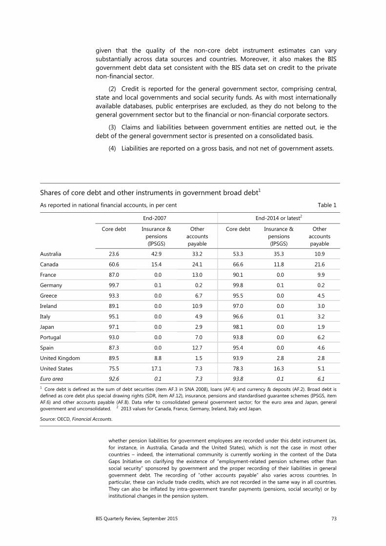
BIS Quarterly Review, September 2015 73
given that the quality of the non-core debt instrument estimates can vary substantially across data sources and countries. Moreover, it also makes the BIS government debt data set consistent with the BIS data set on credit to the private non-financial sector.
(2) Credit is reported for the general government sector, comprising central, state and local governments and social security funds. As with most internationally available databases, public enterprises are excluded, as they do not belong to the general government sector but to the financial or non-financial corporate sectors.
(3) Claims and liabilities between government entities are netted out, ie the debt of the general government sector is presented on a consolidated basis.
(4) Liabilities are reported on a gross basis, and not net of government assets.
whether pension liabilities for government employees are recorded under this debt instrument (as, for instance, in Australia, Canada and the United States), which is not the case in most other countries – indeed, the international community is currently working in the context of the Data Gaps Initiative on clarifying the existence of “employment-related pension schemes other than social security” sponsored by government and the proper recording of their liabilities in general government debt. The recording of ”other accounts payable” also varies across countries. In particular, these can include trade credits, which are not recorded in the same way in all countries. They can also be inflated by intra-government transfer payments (pensions, social security) or by institutional changes in the pension system.
Shares of core debt and other instruments in government broad debt1
As reported in national financial accounts, in per cent Table 1
End-2007 End-2014 or latest2
Core debt Insurance & pensions (IPSGS)
Other accounts payable
Core debt Insurance & pensions (IPSGS)
Other accounts payable
Australia 23.6 42.9 33.2 53.3 35.3 10.9
Canada 60.6 15.4 24.1 66.6 11.8 21.6
France 87.0 0.0 13.0 90.1 0.0 9.9
Germany 99.7 0.1 0.2 99.8 0.1 0.2
Greece 93.3 0.0 6.7 95.5 0.0 4.5
Ireland 89.1 0.0 10.9 97.0 0.0 3.0
Italy 95.1 0.0 4.9 96.6 0.1 3.2
Japan 97.1 0.0 2.9 98.1 0.0 1.9
Portugal 93.0 0.0 7.0 93.8 0.0 6.2
Spain 87.3 0.0 12.7 95.4 0.0 4.6
United Kingdom 89.5 8.8 1.5 93.9 2.8 2.8
United States 75.5 17.1 7.3 78.3 16.3 5.1
Euro area 92.6 0.1 7.3 93.8 0.1 6.1 1 Core debt is defined as the sum of debt securities (item AF.3 in SNA 2008), loans (AF.4) and currency & deposits (AF.2). Broad debt is defined as core debt plus special drawing rights (SDR, item AF.12), insurance, pensions and standardised guarantee schemes (IPSGS, item AF.6) and other accounts payable (AF.8). Data refer to consolidated general government sector; for the euro area and Japan, general government and unconsolidated. 2 2013 values for Canada, France, Germany, Ireland, Italy and Japan.
Source: OECD, Financial Accounts.
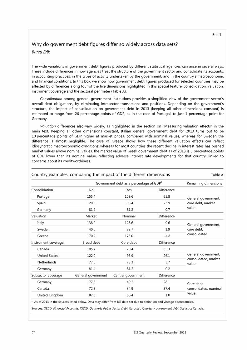
74 BIS Quarterly Review, September 2015
Box 1
Why do government debt figures differ so widely across data sets? Burcu Erik
The wide variations in government debt figures produced by different statistical agencies can arise in several ways. These include differences in how agencies treat the structure of the government sector and consolidate its accounts, in accounting practices, in the types of activity undertaken by the government, and in the country’s macroeconomic and financial conditions. In this box, we show how government debt figures produced for selected countries may be affected by differences along four of the five dimensions highlighted in this special feature: consolidation, valuation, instrument coverage and the sectoral perimeter (Table A).
Consolidation among general government institutions provides a simplified view of the government sector’s overall debt obligations, by eliminating intrasector transactions and positions. Depending on the government’s structure, the impact of consolidation on government debt in 2013 (keeping all other dimensions constant) is estimated to range from 26 percentage points of GDP, as in the case of Portugal, to just 1 percentage point for Germany.
Valuation differences also vary widely, as highlighted in the section on “Measuring valuation effects” in the main text. Keeping all other dimensions constant, Italian general government debt for 2013 turns out to be 10 percentage points of GDP higher at market prices, compared with nominal values, whereas for Sweden the difference is almost negligible. The case of Greece shows how these different valuation effects can reflect idiosyncratic macroeconomic conditions: whereas for most countries the recent decline in interest rates has pushed market values above nominal values, the market value of Greek government debt as of 2013 is 5 percentage points of GDP lower than its nominal value, reflecting adverse interest rate developments for that country, linked to concerns about its creditworthiness.
Country examples: comparing the impact of the different dimensions Table A
Government debt as a percentage of GDP1 Remaining dimensions
Consolidation No Yes Difference
Portugal 155.4 129.6 25.8 General government, core debt, market value
Spain 120.3 96.4 23.9
Germany 81.9 81.2 0.7
Valuation Market Nominal Difference
Italy 138.2 128.6 9.6 General government, core debt, consolidated
Sweden 40.6 38.7 1.9
Greece 170.2 175.0 -4.8
Instrument coverage Broad debt Core debt Difference
Canada 105.7 70.4 35.3 General government, consolidated, market value
United States 122.0 95.9 26.1
Netherlands 77.0 73.3 3.7
Germany 81.4 81.2 0.2
Subsector coverage General government Central government Difference
Germany 77.3 49.2 28.1 Core debt, consolidated, nominal value
Canada 72.3 34.9 37.4
United Kingdom 87.3 86.4 1.0 1 As of 2013 in the sources listed below. Data may differ from BIS data set due to definition and vintage discrepancies.
Sources: OECD, Financial Accounts; OECD, Quarterly Public Sector Debt; Eurostat, Quarterly government debt; Statistics Canada.
BIS Quarterly Review, September 2015 75
The scope of instrument coverage can also affect estimates. In the case of Germany, for example, using the general government’s core debt instead of broad debt would have no significant effect. But the inclusion of non-core debt liabilities would increase government debt by more than 35 percentage points of GDP for Canada. Yet the implied deterioration of Canada’s fiscal position, relative to that of other countries, may be misleading. The unfunded liabilities related to government-sponsored employment-related pension schemes in Canada are included in the financial accounts of the general government, which is in line with the standards and should be positively viewed from a fiscal transparency and sustainability perspective. However, many countries do not record such liabilities explicitly; moreover, there are cross-country discrepancies related to the sectoral classification of such pension schemes (funded or not), which should be in the general government sector when they are controlled by government, but may also be classified as pension funds in the financial corporations sector. In the current reporting, therefore, there are differences due to diverse institutional arrangements among countries. These types of discrepancy explain why the BIS data set focuses on core debt for the purpose of cross-country comparisons.
Finally, there are differences as to which subsectors should be included in debt figures for the general government as a whole, despite the clear recommendations contained in 2008 SNA. Considering just the central government instead of the general government sector reduces 2013 government debt by only 1 percentage point of GDP for the United Kingdom, but by up to 37 percentage points of GDP for Canada.
It should be noted, in addition, that general pension-related contingent liabilities associated with pay-as-you-go social security schemesare not recorded by most other countries. For details on these issues, see 2008 SNA, #17.191–206.
(5) Wherever possible, separate data are reported using two distinct valuation methods: one with the SNA-recommended approach (ie market value whenever possible), and a second with nominal values.
(6) Data are reported at a quarterly frequency.
This BIS concept of core debt, measured at nominal value, is identical to the so-called Maastricht debt,12 which is used in the European Union for the purpose of the Excessive Deficit Procedure (EDP) as well as for the Stability and Growth Pact (SGP).13
The BIS data set has a number of advantages. First, the main benefit of the narrower core debt concept is that the data are available for a larger set of countries and with rather homogeneous characteristics. Certainly, some national discrepancies remain, and the data presented by the BIS may not all have exactly the same targeted features as listed above. But these discrepancies are smaller than for other databases, and the related methodological issues are clearly documented on the website.14
Second, the new BIS data set adds value to existing information by presenting government liabilities whenever possible in both nominal and market value terms (this is the case for 26 of the 40 countries). This can facilitate economic analysis in a number of ways, as when determining the effect of interest rate changes on government debt stocks (see below).
Third, the BIS data report debt levels at a quarterly frequency – whereas most international sources are primarily annual – with a focus on extending the series as far back in time as possible.
12 See Eurostat definition of general government gross debt as defined in the Maastricht Treaty: http://ec.europa.eu/eurostat/en/web/products-data sets/-/TSDDE410.
13 See European Commission (2012). 14 www.bis.org/statistics/totcredit.htm.
76 BIS Quarterly Review, September 2015
Lastly, the new data set on government debt complements the data on credit to the private non-financial sector that the BIS has published since 2013. These two government and private credit data sets rely on identical instrument coverage and are presented in gross terms (although the data set for the private sector is not on a consolidated basis).15 Aggregate data on credit to the non-financial sector are therefore made available in parallel.
One disadvantage of the new government debt data set is that its coverage may be too limited for some purposes. As mentioned earlier, it excludes important financial liabilities that are undoubtedly part of government debt, such as SDR, IPSGS and other accounts payable. In this sense, the BIS data are intended to complement, rather than replace, the other widely used international databases, in particular when precise cross-country comparisons are required. In any case, a careful analysis of a country’s fiscal position should always rely on a wide range of fiscal indicators, including both non-core debt instruments and explicit as well as implicit government contingent guarantees and liabilities (especially those related to ageing and unfunded social security schemes).16
Another limitation is that, for some purposes, net debt may be more appropriate. The main challenges of any netting, however, would be to decide which assets can be deducted from the debt, at what value, and how to handle cross-country differences in valuing government assets.
Measuring valuation effects
Uniquely, the new BIS data set tracks the evolution of government core debt at nominal and market value.
Market value is the amount for which a creditor could exchange assets or settle a liability at any moment in time.17 In particular, changes in the market value of debt affect the financial position of investors that mark their portfolios to market or monitor market values in order to assess potential gains or losses. Market values may fluctuate significantly because of changes in risk-free interest rates, but also in credit and other risk premia.
In contrast, the nominal value of a debt instrument, ie “the amount that at any moment in time the debtor owes to the creditor” (Handbook on Securities Statistics; see BIS-ECB-IMF (2015)), is stable from the moment of issuance till full repayment (except when accrued interest has not yet been paid; see below). The difference between the market and nominal value of a security reflects changes in yields since issuance.
15 This apparent inconsistency between the private and government debt data sets is warranted, since one single entity is usually “responsible” for the operations of the government sector, although the appropriateness of this assumption depends on country-specific factors. In contrast, netting credit relationships within the private non-financial sector would be misleading for debt sustainability assessment, since intrasector financial flows can be large and may have destabilising systemic effects, as seen in the last financial crisis (Dembiermont et al (2013)).
16 See eg Carnot et al (2011) for an overview of the issues related to fiscal policy analysis. 17 Market value is “the price at which debt securities are acquired or disposed of in transactions
between willing parties, excluding commissions, fees, and taxes, but including accrued interest” (Handbook on Securities Statistics).

BIS Quarterly Review, September 2015 77
In cases where nominal values are not available, face values are commonly used. These concepts are close but not identical. Nominal value consists of the sum of funds originally advanced, plus any subsequent advances less any repayments, plus any accrued interest not yet paid; face value (also known as “par18 value” or simply “par”) refers only to the principal amount to be repaid at maturity (2008 SNA and Handbook on Securities Statistics). To illustrate the differences implied by these valuation definitions, Table 2 shows an example of a five-year fixed interest rate bond issued at par with annual coupon payments of 10%, as taken from the Handbook on Securities Statistics.
In this example, the face value of the bond is constant at 1,000 throughout its life. Its nominal value ranges from 1,000 to 1,100 throughout each year, depending on the elapsed time since last coupon payment and thus the amount of interest accrued (but not yet paid). The market value of the bond, however, is influenced not only by the treatment of accrued interest, but also by changes in market interest rates (ie the market value increases as the market interest rate falls, raising the present value of future coupon and principal payments, and vice versa when the interest rate rises). The Handbook on Securities Statistics (Annex 1) provides additional detailed examples for other types of bonds.
The market and nominal value concepts provide complementary perspectives. Generally, market values provide information on the relative size and depth of different markets, the value of collateral or the investors’ exposure to government. Nominal values are particularly useful for some types of debt sustainability analysis (eg the effect of interest rate changes on debt servicing).
When data sets on government core debt are comparable and available in both market and nominal value terms, debt valuation effects can be readily monitored. This is useful in tracking the impact of, say, changes in interest rates and yields, including those driven by market participants’ perceptions of creditworthiness.
18 A bond trades “at par“ when its nominal and market value are the same (ie the yield equals the coupon and the investor expects the same return).
Valuations of a five-year fixed interest rate bond issued at par during its life Table 2
Start Q1 End Q1 End Q2 End Q3 Up to end Q4
End Q4 = start
Q5
End year 2
End year 3
End year 4
End year 5
Face value 1,000.0 1,000.0 1,000.0 1,000.0 1,000.0 1,000.0 1,000.0 1,000.0 1,000.0 1,000.0
Nominal value 1,000.0 1,024.1 1,048.8 1,074.1 1,100.0 1,000.0 1,000.0 1,000.0 1,000.0 1,000.0
Accrued interest – 24.1 48.8 74.1 100.0 – – – – –
Coupon payment – – – – –100.0 – – – – –
Market interest rate (per annum)
10 10 10 10 10 11 9 7 12 8
Market value 1,000.01 1,024.1 1,048.8 1,074.1 1,100.0 969.0 1,025.3 1,054.2 982.1 1,000.0 1 The market value of the bond at the beginning of the first year, where the market interest rate is 10%, is equal to the sum of the present value of the principal to be received at the end of year 5 ie . and the present value of the future annual coupon payments ie . +. + . + . + . . If interest rates move to 11% just after issuance, then the market value becomes 963 ie . + . + . + . +. + . .
Source: Handbook on Securities Statistics, derived from Box 5.1 and Annex 1.
78 BIS Quarterly Review, September 2015
Graph 2 and Table 3 present market and nominal values of government core debt relative to GDP, as well as the valuation effect (estimated simply as the difference between the two), for a selected group of 12 countries and the euro area.19 It is clear, first, that government debt (both market and nominal values) has been rising strongly for most countries since the crisis. Second, market values have outpaced nominal values in most cases due to falling interest rates. Before the beginning of the financial crisis in 2007, credit to the government valued at market prices was already more than 2 percentage points of GDP higher than at nominal value, on average, for this group of 12 countries. This average gap between nominal and market values had widened to 9 percentage points of GDP by end-2014 – reaching a level as high as 19 and 18 percentage points of GDP for Italy and theUnited Kingdom, respectively. In some countries, especially Canada, Germany and Ireland, core debt appears to have started declining recently when measured at nominal value, while the change is much smaller when looking at market values (Graph 2).
Box 2
Where do the data come from?
Government debt data at nominal value are derived mainly from government fiscal indicators compiled by the agencies responsible for public finance management or national statistical institutes. In Europe, the statistical office of the European Union, Eurostat, provides data on the so-called Maastricht debt, which corresponds to the BIS target definition of government core debt in terms of instrument and sector coverage, consolidation and netting. For example, in the euro area at the end of Q4 2014, Maastricht debt was 91.9 % of GDP, which is identical to the BIS core debt figure (using nominal value).
Credit figures at market value are provided by data on the balance sheet of the government sector that are included in the sectoral financial accounts. These financial accounts form part of the 2008 SNA and are sometimes also labelled as the “Flow of funds” (FOF). However, some countries have not yet begun to compile financial accounts and typically record their debt liabilities at nominal value in their fiscal accounts. This explains why fewer countries are listed in the BIS market value data set than in the nominal value one.
For cases where it is not possible to retrieve data that already have the features targeted by the BIS, partial information can be mobilised to complement missing financial accounts data. Data on debt securities issued by the general government are a case in point. As argued in the main text (“Measuring valuation effects”), debt securities account for the main difference between the market and nominal values of core debt estimates. In the United States, for instance, the debt securities are compiled in the FOF at face value, and are made only partially available at market value by the Federal Reserve Bank of Dallas. The BIS market value data set is constructed by extrapolating these figures for the whole government sector. By contrast, in Australia, government debt data are published only at market value. To construct BIS nominal core debt estimates, figures from the financial accounts have to be replaced by data on debt securities at nominal value as reported by the Australian Office of Financial Management. In Canada, to offer yet another example, consolidated core debt at nominal value is derived from unconsolidated data, using information provided at market value for both the consolidated and the unconsolidated general government core debt figures. For Japan, both market and face values of outstanding debt securities are reported in the FOF, but the general government sector is not consolidated. Inter-government claims, to the extent that they can be identified in the financial accounts, must therefore be removed from the debt data in order to arrive at an estimate for the consolidated sector.
The Maastricht debt concept is measured at nominal (face) value. See European Council regulation no 479/2009 of 25 May 2009.
19 See also BIS (2015).

BIS Quarterly Review, September 2015 79
General government core debt: valuation effects1
As a percentage of GDP Graph 2
Canada France Germany Greece
Ireland Italy Japan Portugal
Spain United Kingdom United States Euro area
1 Debt levels at market value refer to consolidated core debt, which covers debt securities, loans and currency & deposits. Valuation effectsare estimates of the difference between debt securities valuations at market prices and nominal prices. The valuation effect is estimated simply as the difference between the reported market and nominal values of consistent debt aggregates.
Sources: ECB; Eurostat; national data; BIS estimates.
For given changes in market interest rates, the valuation effect increases with the maturity (or, strictly speaking, the duration)20 of the corresponding debt
20 Duration being “the weighted average term to maturity of a debt instrument” (Handbook on Securities Statistics).
40
50
60
70
80
0
5
10
15
20
07 09 11 13 15
60
75
90
105
120
0
5
10
15
20
07 09 11 13 15
50
60
70
80
90
–5
0
5
10
15
07 09 11 13 15
80
100
120
140
160
–80
–60
–40
–20
0
07 09 11 13 15
0
30
60
90
120
–20
–10
0
10
20
07 09 11 13 15
90
105
120
135
150
–5
0
5
10
15
07 09 11 13 15
140
160
180
200
220
–5
0
5
10
15
07 09 11 13 15
60
80
100
120
140
–20
–10
0
10
20
07 09 11 13 15
20
40
60
80
100
–5
0
5
10
15
07 09 11 13 15
Market value (lhs)
20
40
60
80
100
0
5
10
15
20
07 09 11 13 15
Nominal value (lhs)
45
60
75
90
105
0
5
10
15
20
07 09 11 13 15
Valuation effects (rhs)
60
75
90
105
120
0
5
10
15
20
07 09 11 13 15
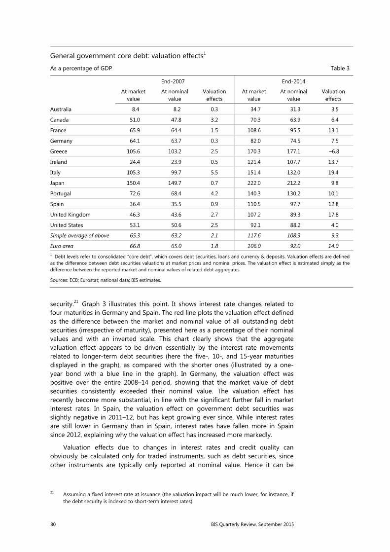
80 BIS Quarterly Review, September 2015
security.21 Graph 3 illustrates this point. It shows interest rate changes related to four maturities in Germany and Spain. The red line plots the valuation effect defined as the difference between the market and nominal value of all outstanding debt securities (irrespective of maturity), presented here as a percentage of their nominal values and with an inverted scale. This chart clearly shows that the aggregate valuation effect appears to be driven essentially by the interest rate movements related to longer-term debt securities (here the five-, 10-, and 15-year maturities displayed in the graph), as compared with the shorter ones (illustrated by a one-year bond with a blue line in the graph). In Germany, the valuation effect was positive over the entire 2008–14 period, showing that the market value of debt securities consistently exceeded their nominal value. The valuation effect has recently become more substantial, in line with the significant further fall in market interest rates. In Spain, the valuation effect on government debt securities was slightly negative in 2011–12, but has kept growing ever since. While interest rates are still lower in Germany than in Spain, interest rates have fallen more in Spain since 2012, explaining why the valuation effect has increased more markedly.
Valuation effects due to changes in interest rates and credit quality can obviously be calculated only for traded instruments, such as debt securities, since other instruments are typically only reported at nominal value. Hence it can be
21 Assuming a fixed interest rate at issuance (the valuation impact will be much lower, for instance, if the debt security is indexed to short-term interest rates).
General government core debt: valuation effects1
As a percentage of GDP Table 3
End-2007 End-2014
At market value
At nominal value
Valuation effects
At market value
At nominal value
Valuation effects
Australia 8.4 8.2 0.3 34.7 31.3 3.5
Canada 51.0 47.8 3.2 70.3 63.9 6.4
France 65.9 64.4 1.5 108.6 95.5 13.1
Germany 64.1 63.7 0.3 82.0 74.5 7.5
Greece 105.6 103.2 2.5 170.3 177.1 –6.8
Ireland 24.4 23.9 0.5 121.4 107.7 13.7
Italy 105.3 99.7 5.5 151.4 132.0 19.4
Japan 150.4 149.7 0.7 222.0 212.2 9.8
Portugal 72.6 68.4 4.2 140.3 130.2 10.1
Spain 36.4 35.5 0.9 110.5 97.7 12.8
United Kingdom 46.3 43.6 2.7 107.2 89.3 17.8
United States 53.1 50.6 2.5 92.1 88.2 4.0
Simple average of above 65.3 63.2 2.1 117.6 108.3 9.3
Euro area 66.8 65.0 1.8 106.0 92.0 14.0 1 Debt levels refer to consolidated “core debt”, which covers debt securities, loans and currency & deposits. Valuation effects are defined as the difference between debt securities valuations at market prices and nominal prices. The valuation effect is estimated simply as the difference between the reported market and nominal values of related debt aggregates.
Sources: ECB; Eurostat; national data; BIS estimates.

BIS Quarterly Review, September 2015 81
argued that these effects are underestimated to the extent that a significant share of government debt takes the form of loans rather than securities.
The United Kingdom and Ireland are good illustrations of this point. In the United Kingdom, interest rates dropped less in recent years than did those in Germany or Spain (Graph 4), but the measured valuation effect was significantly higher (18 percentage points of GDP compared with 8 for Germany; see Table 4). This can be explained at least in part by the higher share of debt securities within UK government core debt (compared with German debt), while the higher remaining maturity of UK government debt securities also played a role (Table 4). In Ireland, the relatively low share of debt securities has dampened the substantial revaluation impact due to the significant post-crisis fall in interest rates.
Interest rate developments and debt securities market valuation effects
In per cent Graph 3
Germany Spain
1 Difference between the market and nominal value of all outstanding government debt securities, as a percentage of the nominal value.
Sources: ECB; Bloomberg.
Ten-year government bond yields
In per cent Graph 4
Source: National data.
–2
0
2
4
6 0
6
12
18
24
2008 2009 2010 2011 2012 2013 2014
Lhs: 1-year yields5-year yields
10-year yields15-year yields
–2
0
2
4
6 0
6
12
18
24
2009 2010 2011 2012 2013 2014
Valuation effect on debt securities1 (rhs, inverted scale)
0
8
16
24
0
4
8
12
2008 2009 2010 2011 2012 2013 2014 2015
GreeceLhs:
GermanyRhs:
Ireland Spain United Kingdom
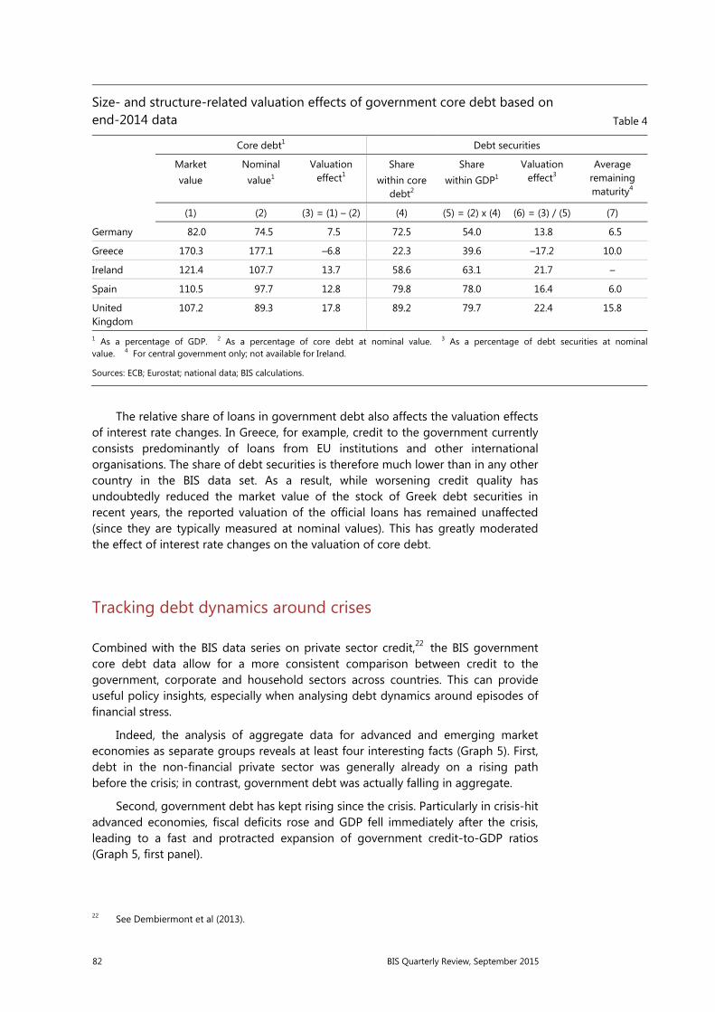
82 BIS Quarterly Review, September 2015
The relative share of loans in government debt also affects the valuation effects of interest rate changes. In Greece, for example, credit to the government currently consists predominantly of loans from EU institutions and other international organisations. The share of debt securities is therefore much lower than in any other country in the BIS data set. As a result, while worsening credit quality has undoubtedly reduced the market value of the stock of Greek debt securities in recent years, the reported valuation of the official loans has remained unaffected (since they are typically measured at nominal values). This has greatly moderated the effect of interest rate changes on the valuation of core debt.
Tracking debt dynamics around crises
Combined with the BIS data series on private sector credit,22 the BIS government core debt data allow for a more consistent comparison between credit to the government, corporate and household sectors across countries. This can provide useful policy insights, especially when analysing debt dynamics around episodes of financial stress.
Indeed, the analysis of aggregate data for advanced and emerging market economies as separate groups reveals at least four interesting facts (Graph 5). First, debt in the non-financial private sector was generally already on a rising path before the crisis; in contrast, government debt was actually falling in aggregate.
Second, government debt has kept rising since the crisis. Particularly in crisis-hit advanced economies, fiscal deficits rose and GDP fell immediately after the crisis, leading to a fast and protracted expansion of government credit-to-GDP ratios (Graph 5, first panel).
22 See Dembiermont et al (2013).
Size- and structure-related valuation effects of government core debt based on end-2014 data Table 4
Core debt1 Debt securities
Market value
Nominal value1
Valuation effect1
Share within core
debt2
Share within GDP1
Valuation effect3
Average remaining maturity4
(1) (2) (3) = (1) – (2) (4) (5) = (2) x (4) (6) = (3) / (5) (7)
Germany 82.0 74.5 7.5 72.5 54.0 13.8 6.5
Greece 170.3 177.1 –6.8 22.3 39.6 –17.2 10.0
Ireland 121.4 107.7 13.7 58.6 63.1 21.7 –
Spain 110.5 97.7 12.8 79.8 78.0 16.4 6.0
United Kingdom
107.2 89.3 17.8 89.2 79.7 22.4 15.8
1 As a percentage of GDP. 2 As a percentage of core debt at nominal value. 3 As a percentage of debt securities at nominal value. 4 For central government only; not available for Ireland.
Sources: ECB; Eurostat; national data; BIS calculations.
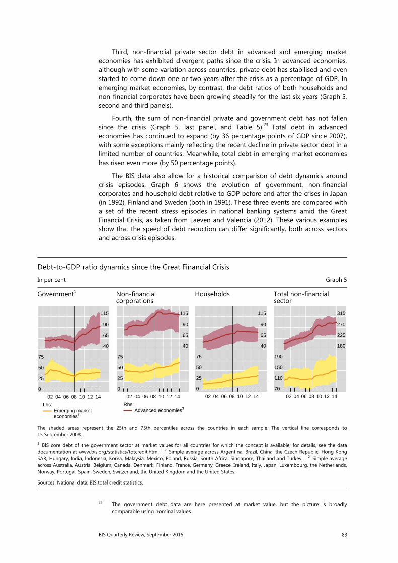
BIS Quarterly Review, September 2015 83
Third, non-financial private sector debt in advanced and emerging market economies has exhibited divergent paths since the crisis. In advanced economies, although with some variation across countries, private debt has stabilised and even started to come down one or two years after the crisis as a percentage of GDP. In emerging market economies, by contrast, the debt ratios of both households and non-financial corporates have been growing steadily for the last six years (Graph 5, second and third panels).
Fourth, the sum of non-financial private and government debt has not fallen since the crisis (Graph 5, last panel, and Table 5).23 Total debt in advanced economies has continued to expand (by 36 percentage points of GDP since 2007), with some exceptions mainly reflecting the recent decline in private sector debt in a limited number of countries. Meanwhile, total debt in emerging market economies has risen even more (by 50 percentage points).
The BIS data also allow for a historical comparison of debt dynamics around crisis episodes. Graph 6 shows the evolution of government, non-financial corporates and household debt relative to GDP before and after the crises in Japan (in 1992), Finland and Sweden (both in 1991). These three events are compared with a set of the recent stress episodes in national banking systems amid the Great Financial Crisis, as taken from Laeven and Valencia (2012). These various examples show that the speed of debt reduction can differ significantly, both across sectors and across crisis episodes.
23 The government debt data are here presented at market value, but the picture is broadly comparable using nominal values.
Debt-to-GDP ratio dynamics since the Great Financial Crisis
In per cent Graph 5
Government1 Non-financialcorporations
Households Total non-financial sector
The shaded areas represent the 25th and 75th percentiles across the countries in each sample. The vertical line corresponds to15 September 2008.
1 BIS core debt of the government sector at market values for all countries for which the concept is available; for details, see the data documentation at www.bis.org/statistics/totcredit.htm. 2 Simple average across Argentina, Brazil, China, the Czech Republic, Hong Kong SAR, Hungary, India, Indonesia, Korea, Malaysia, Mexico, Poland, Russia, South Africa, Singapore, Thailand and Turkey. 2 Simple average across Australia, Austria, Belgium, Canada, Denmark, Finland, France, Germany, Greece, Ireland, Italy, Japan, Luxembourg, the Netherlands,Norway, Portugal, Spain, Sweden, Switzerland, the United Kingdom and the United States.
Sources: National data; BIS total credit statistics.
0
25
50
75
40
65
90
115
02 04 06 08 10 12 14
Emerging marketeconomies2
Lhs:
0
25
50
75
40
65
90
115
02 04 06 08 10 12 14
Advanced economies3Rhs:
0
25
50
75
40
65
90
115
02 04 06 08 10 12 14
70
110
150
190
180
225
270
315
02 04 06 08 10 12 14
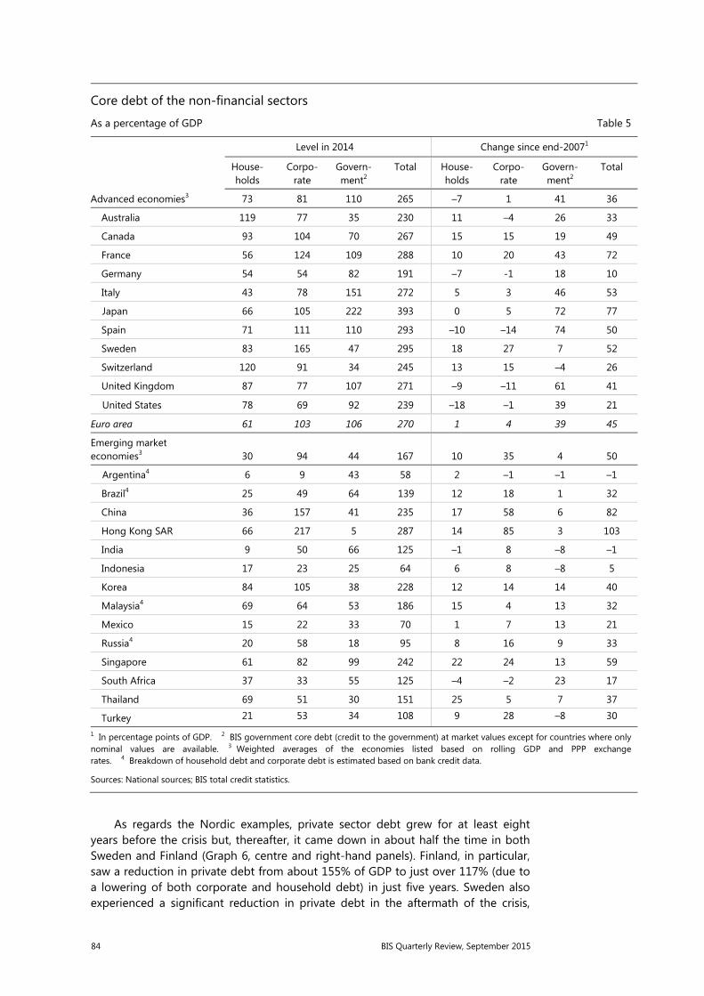
84 BIS Quarterly Review, September 2015
Core debt of the non-financial sectors
As a percentage of GDP Table 5
Level in 2014 Change since end-20071
House-holds
Corpo-rate
Govern-ment2
Total House-holds
Corpo-rate
Govern-ment2
Total
Advanced economies3 73 81 110 265 –7 1 41 36
Australia 119 77 35 230 11 –4 26 33
Canada 93 104 70 267 15 15 19 49
France 56 124 109 288 10 20 43 72
Germany 54 54 82 191 –7 -1 18 10
Italy 43 78 151 272 5 3 46 53
Japan 66 105 222 393 0 5 72 77
Spain 71 111 110 293 –10 –14 74 50
Sweden 83 165 47 295 18 27 7 52
Switzerland 120 91 34 245 13 15 –4 26
United Kingdom 87 77 107 271 –9 –11 61 41
United States 78 69 92 239 –18 –1 39 21
Euro area 61 103 106 270 1 4 39 45
Emerging market economies3 30 94 44 167 10 35 4 50
Argentina4 6 9 43 58 2 –1 –1 –1
Brazil4 25 49 64 139 12 18 1 32
China 36 157 41 235 17 58 6 82
Hong Kong SAR 66 217 5 287 14 85 3 103
India 9 50 66 125 –1 8 –8 –1
Indonesia 17 23 25 64 6 8 –8 5
Korea 84 105 38 228 12 14 14 40
Malaysia4 69 64 53 186 15 4 13 32
Mexico 15 22 33 70 1 7 13 21
Russia4 20 58 18 95 8 16 9 33
Singapore 61 82 99 242 22 24 13 59
South Africa 37 33 55 125 –4 –2 23 17
Thailand 69 51 30 151 25 5 7 37
Turkey 21 53 34 108 9 28 –8 30
1 In percentage points of GDP. 2 BIS government core debt (credit to the government) at market values except for countries where only nominal values are available. 3 Weighted averages of the economies listed based on rolling GDP and PPP exchange rates. 4 Breakdown of household debt and corporate debt is estimated based on bank credit data.
Sources: National sources; BIS total credit statistics.
As regards the Nordic examples, private sector debt grew for at least eight years before the crisis but, thereafter, it came down in about half the time in both Sweden and Finland (Graph 6, centre and right-hand panels). Finland, in particular, saw a reduction in private debt from about 155% of GDP to just over 117% (due to a lowering of both corporate and household debt) in just five years. Sweden also experienced a significant reduction in private debt in the aftermath of the crisis,

BIS Quarterly Review, September 2015 85
though to a lesser extent. Both Sweden and Finland recorded sharp increases in government sector debt ratios immediately after the crisis. This reflected the strain on public finances of bailing out the financial system as well as the effect of output losses on fiscal revenues. But these government ratios started to come down noticeably once most of the deleveraging of the private sector had been completed.
The example of Japan was quite different. Private sector deleveraging was more muted after the crisis, and was mainly concentrated in the non-financial corporate sector. Household debt as a percentage of GDP continued to rise slightly several years after the crisis and did not correct afterwards. Initially, government debt rose less rapidly than it did in the Nordic cases, not least since the repair of banks’ balance sheets started much later, but the government debt position continued to worsen for much longer and ended up much larger.
Turning now to the 2007–08 examples, Graph 6 shows that, seven years into the latest financial crisis, debt reduction seems to have only just started. There are certainly important differences between countries, with for example a somewhat quicker paydown of debt in the United States and the United Kingdom. In aggregate, however, the debt dynamics of the advanced economies resemble more the pattern of those of Japan in the early 1990s than of the Nordic countries in 1991. Aggregate private debt has barely stabilised, let alone started to correct downwards, even in the corporate sector. And government debt continues to rise steadily, in a manner reminiscent of Japan’s trend deterioration in the 1990s – and unlike the large but temporary deterioration followed by a rapid improvement in fiscal positions experienced by the Nordic states during the same period.
Debt-to-GDP ratio dynamics during past debt reduction episodes
Year of the crisis = 100 Graph 6
Government Non-financial corporates Households
Year of the crisis in parentheses. The line for all countries is a simple average including the following episodes: Austria (2008); Belgium (2008); Denmark (2008); France (2008); Germany (2008); Greece (2008); Hungary (2008); Ireland (2008); Italy (2008); the Netherlands (2008); Portugal (2008); Russia (2008); Spain (2008); Sweden (2008); Switzerland (2008); the United Kingdom (2007); the United States (2007).
Sources: Laeven and Valencia (2012); IMF, World Economic Outlook; OECD, Economic Outlook; national data; BIS total credit statistics.
40
70
100
130
160
190
220
250
–10 –8 –6 –4 –2 0 2 4 6 8 10Years (crisis = 0)
All countries (2007–08)
40
60
80
100
120
–10 –8 –6 –4 –2 0 2 4 6 8 10Years (crisis = 0)
Finland (1991) Sweden (1991)
40
60
80
100
120
–10 –8 –6 –4 –2 0 2 4 6 8 10Years (crisis = 0)
Japan (1992)
86 BIS Quarterly Review, September 2015
Conclusions
The new data set on government debt for 26 advanced and 14 emerging market economies presented in this special feature has three main objectives. First, the definition and coverage of these indicators is consistent across countries, facilitating cross-country comparisons, and with a relatively high (quarterly) frequency.
Second, the underlying concepts are also consistent with those used to build the existing BIS data set on credit to the non-financial private sector, publicly available since 2013. As a result, BIS data now support the analysis of country debt patterns at the level of both subsectors and the entire non-financial sector.
Third, a key distinctive feature of the government debt data set is that it contains series expressed in both nominal and market terms. The latter feature appears particularly topical at present when large changes in interest rates – owing to the trend decline in benchmark yields and changing perceptions of sovereign creditworthiness – have increased the size of valuation effects.
The new BIS data sets support the analysis of credit developments both by region and by sector. These data show that non-financial private sector indebtedness was already on the rise before the Great Financial Crisis, while the reduction in government debt was quite modest in comparison. In the most crisis-hit advanced economies, government debt started to rise after 2008 at an especially fast and persistent pace. At the same time, private sector credit has barely stabilised, even if it has started to edge downwards noticeably in a few jurisdictions. The combined effect of these developments (minor private deleveraging, sharp deterioration in fiscal positions) has been a further increase in total debt in the advanced economies’ non-financial sectors from 229% of GDP on average in 2007 to 265% in 2014 (using PPP weights). Turning to emerging market economies, we see that government debt has been relatively stable on average, while non-financial private debt has been on the increase for the last seven years. As a result, the total credit-to-GDP ratio went from 117% to 167% for this group of economies.

BIS Quarterly Review, September 2015 87
References
Avdjiev, S, P McGuire and P Wooldridge (2015): “Enhanced data to analyse international banking”, BIS Quarterly Review, September, pp 53–68.
Bank for International Settlements (2015): 85th Annual Report, June, Chapter I.
Bank for International Settlements, Commonwealth Secretariat, European Central Bank, European Commission-Eurostat, International Monetary Fund, Organisation for Economic Co-operation and Development, Paris Club Secretariat, United Nations Conference on Trade and Development and World Bank (2011): Public sector debt statistics: Guide for compilers and users.
Bank for International Settlements, European Central Bank and International Monetary Fund (2015): Handbook on Securities Statistics.
Bloch, D and F Fall (2015): “Government debt indicators: understanding the data”, OECD Economics Department Working Papers, no 1228, June.
Carnot, N, V Koen and B Tissot (2011): Economic forecasting and policy, second edition, Palgrave Macmillan, Chapter 5.
Dembiermont C, M Drehmann and S Muksakunratana (2013): “How much does the private sector really borrow – a new database for total credit to the private non-financial sector”, BIS Quarterly Review, March, pp 65–81.
Dippelsman, R, C Dziobek and C Gutiérrez Mangas (2012): “What lies beneath: the statistical definition of public sector debt”, IMF Staff Discussion Notes, SDN/12/09, July.
European Commission (2012): “European Commission scoreboard for the surveillance of macroeconomic imbalances”, European Economy Occasional Papers, no 92.
European Commission, International Monetary Fund, Organisation for Economic Co-operation and Development, United Nations and World Bank (2009): System of National Accounts 2008.
Eurostat, definition of general government gross debt defined in the Maastricht Treaty, http://ec.europa.eu/eurostat/en/web/products-data sets/-/TSDDE410.
International Monetary Fund (2000): Monetary and Financial Statistics Manual.
——— (2014): Government Finance Statistics Manual.
International Monetary Fund and Financial Stability Board (2009): The financial crisis and information gaps – report to the G20 Finance Ministers and Central Bank Governors.
Laeven, L and F Valencia (2012): “Systemic banking crises database: an update”, IMF Working Papers, no 12/163, June.


BIS Quarterly Review, September 2015 89
Mathias Drehmann
Anamaria Illes
Mikael Juselius
Marjorie Santos
How much income is used for debt payments? A new database for debt service ratios1
Debt service ratios (DSRs) provide important information about the interactions between debt and the real economy, as they measure the amount of income used for interest payments and amortisations. Given this pivotal role, the BIS has started to produce and release aggregate DSRs for the total private non-financial sector for 32 countries from 1999 onwards. For the majority of countries, DSRs for the household and the non-financial corporate sectors are also available. This article explains the key concepts underlying the compilation of the new series and it shows that the DSRs are meaningful, even when derived from a relatively sparse set of aggregate data. A brief look at the evolution of DSRs in recent years highlights that they allow for a more comprehensive assessment of credit burdens than the credit-to-income ratio or simple measures of interest payments relative to income.
JEL classification: C8, E50.
Debt forms a central part of the narrative of financial crises and financial cycles more generally. Leverage, often proxied at the aggregate level by the ratio of the stock of liabilities (ie debt) to income, has received much attention as an indicator of financial excesses and vulnerabilities. Less discussed, but equally important, is the debt service ratio (DSR), which captures the share of income used for interest payments and amortisations. These debt-related flows are a direct result of previous borrowing decisions and often move slowly as they depend on the duration and other terms of credit contracts. They have a direct impact on borrowers’ budget constraints and thus affect spending.
Since the DSR captures the link between debt-related payments and spending, it is a crucial variable for understanding the interactions between debt and the real economy. For instance, during financial booms, increases in asset prices boost the value of collateral, making borrowing easier. But more debt means higher debt service ratios, especially if interest rates rise. This constrains spending, which offsets the boost from new lending, and the boom runs out of steam at some point. After a financial bust, it takes time for debt service ratios, and thus spending, to normalise even if interest rates fall, as principal still needs to be paid down. In fact, the evolution of debt service burdens can explain the dynamics of US spending in the
1 We would like to thank Christian Dembiermont, whose statistical knowledge was invaluable for the compilation of the series. We are also grateful for input from national central banks. This article benefited from useful comments by Claudio Borio, Ben Cohen, Dietrich Domanski, Hyun Song Shin and Suresh Sundaresan. The views expressed in it are those of the authors and do not necessarily reflect those of the BIS.
90 BIS Quarterly Review, September 2015
aftermath of the Great Financial Crisis fairly well.2 In addition, DSRs are also highly reliable early warning indicators of systemic banking crises.3
Given this pivotal role, the BIS has started to produce and release aggregate DSRs for the total private non-financial sector on a regular basis.4 The new DSR database currently covers quarterly series for 32 countries from 1999 onwards. For the majority of countries, series for the household and the non-financial corporate (NFC) sectors are also available. To derive the DSR on an internationally consistent basis, we apply a unified methodological approach and use, as far as they are available, input data that are compiled on an internationally consistent basis.
The methodology, the data inputs and some results are discussed in the remainder of this article.
Methodology
The DSR is defined as the ratio of interest payments plus amortisations to income. As such, the DSR provides a flow-to-flow comparison – the flow of debt service payments divided by the flow of income.
At the individual level, it is straightforward to determine the DSR. Households and firms know the amount of interest they pay on all their outstanding debts, how much debt they have to amortise per period and how much income they earn. But even so, difficulties can arise. Many contracts can be rolled over so that the effective period for repaying a particular loan can be much longer than the contractual maturity of the specific contract. Equally, some contracts allow for early repayments so that households or firms can amortise ahead of schedule. Given this, deriving aggregate DSRs from individual-level data does not necessarily lead to good estimates.5 And such data are rarely comprehensive, if available at all. For this reason, we derive aggregate DSRs from aggregate data directly.
While interest payments and income are recorded in the national accounts, amortisation data are generally not available and hence present the main difficulty in deriving aggregate DSRs. To overcome this problem, we follow an approach used by the Federal Reserve Board to construct debt service ratios for the household sector (Dynan et al (2003)) which measures amortisations indirectly. It starts with the basic assumption that, for a given lending rate, debt service costs – interest payments and amortisations – on the aggregate debt stock are repaid in equal portions over the maturity of the loan (instalment loans). The justification for this
2 See Juselius and Drehmann (2015) for a formal analysis. 3 See Alessi et al (2014) or Drehmann and Juselius (2014). 4 The series are available on the BIS website at www.bis.org/statistics/dsr.htm. 5 Consider an example of a household that buys a house and borrows CHF 500,000. The initial
mortgage contract runs over 10 years. But the loan is structured on the premise that the borrower can refinance it after 10 years and that he will pay it back in full over a 25-year period. It then makes sense to estimate the DSR under the assumption that the loan has a 25-year maturity. But this may not be known when constructing aggregate DSRs from micro data. In addition, recorded repayment flows may not reflect actual amortisations. For example, after 10 years the household changes its mortgage provider, repaying the original bank CHF 320,000 in year 10, but financing CHF 300,000 of this amount with a new loan from a different bank. Micro-level data might record a repayment of CHF 320,000, even though the repayment by the household is CHF 20,000.
BIS Quarterly Review, September 2015 91
assumption is that the differences between the repayment structures of individual loans will tend to cancel out in the aggregate.6 Using some simulations, we show in Box 1 that this indeed seems to be the case. For instance, approximating the aggregate DSR with the instalment loan formula works, though with a small approximation error, even if the majority of borrowers pay back the principal only at the end of the contract.
By using the standard formula for the per-period cost of an instalment loan (see Box 2 for a derivation) and dividing it by income, the aggregate DSR for sector j at time t can be calculated as:
, = ,1 − 1 + , , ∗ ,, (1)
where Dj,t denotes the total stock of debt, Yj,t denotes aggregate income available for debt service payments, ij,t denotes the average interest rate on the existing stock of debt and sj,t denotes the average remaining maturity across the stock of debt. Given that the new database has a quarterly frequency, we match flows to flows on a quarterly basis. Thus, we use quarterly income and the average interest rate per quarter, and we measure the remaining maturities in quarters.
The instalment loan formula indirectly captures amortisations through the non-linear interest rate term in the denominator. To provide some understanding of how amortisations affect the DSR as interest rates and maturities change, consider a simple example with two sectors, each with a stock of debt of 100 and income of 100. In both sectors, the average remaining maturity of the debt stock is 10 years, but sector A has borrowed at an average interest rate of 2%, whilst sector B has an average interest rate of 5%. Given the interest rate differential, one would expect a substantially lower debt service ratio in sector A. This is not the case, however, because of amortisations. In fact, despite interest payments being 60% lower in sector A, its DSR is only slightly smaller: 11%, compared with 13% in sector B. Now consider a third sector, C, which is similar to sector B in that it also has a debt-to-income ratio of 100% and borrows at an average interest rate of 5%, but it faces an average remaining maturity of only six years. In this case, its DSR is close to 20% rather than 13%. These non-linear effects are illustrated further in Graph 1, which shows hypothetical DSRs for a debt-to-income ratio of 100% over a range of interest rates (Graph 1, left-hand panel) and remaining maturities (Graph 1, right-hand panel).
A potential concern with the instalment loan formula is that the non-linear effects from the “amortisations” term can generate an approximation error when aggregate data are used. For example, applying formula (1) to individual loans and summing up does not produce the same DSR which would be obtained from applying it to aggregate data inputs directly. Nevertheless, this approximation error turns out to be relatively independent of average interest rates, debt-to-income ratios or maturities (Box 1). Thus, our methodology should correctly capture how the DSR in a particular country changes over time, even if it does not necessarily accurately measure its level relative to what one could obtain from the correct micro data. The Fed encountered similar issues in relation to its household DSRs, pointing
6 This aggregation assumption is also intuitive. For example, consider 10 loans of equal size for which the entire interest payment and principal are due at maturity, each with 10 repayment periods and taken out in successive years over a decade. After 10 periods, when the first loan falls due, the flow of interest payments and amortisations on these 10 loans will jointly be indistinguishable from the repayment of a single large instalment loan.

92 BIS Quarterly Review, September 2015
out that its “approximation is useful to the extent that, by using the same method and data series over time, it generates a time series that captures the important changes in the household debt service burden” (Federal Reserve Board (2013)).
Data inputs for constructing DSRs
The previous section has shown that it is possible to construct meaningful aggregate DSRs with a relatively sparse set of aggregate data: the total stock of debt, the income available for debt service payments, the average interest rate on the existing stock of debt and the average remaining maturity. This is encouraging and simplifies our task considerably because it lessens the need for micro-level data, which are not available for a large range of countries and time periods.
This section provides a high-level overview of the data inputs. Further details and country-specific information are provided in the data documentation.7 To ensure international consistency, we rely as much as possible on data from national accounts. In particular, national accounts provide us with information about the stock of debt, income and interest rates.8
We measure the stock of debt for each sector by its credit counterpart as recorded in the BIS database on credit to the private non-financial sector (Dembiermont et al (2013)).
To capture the income available to service the debts of households or non-financial corporations (NFCs), we augment gross disposable income (GDI) with gross interest payments, as GDI measures income after such payments. In the case of
7 See www.bis.org/statistics/dsr.htm. 8 For 15 countries in the sample, only the DSR for the total private non-financial sector (PNFS) is
currently available given data availability. In these cases, income is proxied by nominal quarterly GDP series and the interest rate is proxied by the average interest rate on loans made by banks to the PNFS.
The impact of interest rates and remaining maturities on DSRs1
In per cent Graph 1
DSR levels by changing interest rates DSR levels by changing average remaining maturity
1 Hypothetical DSRs for a debt-to-income ratio of 100% given various interest rates and remaining maturities. When interest rates change,we assume remaining maturities of 10 years. When the remaining maturities change, interest rates are held constant at 5%.
Source: BIS estimates.
0
5
10
15
1 2 3 4 5 6 7 8 9 10Interest rate, in per cent
0
5
10
15
6 7 8 9 10 11 12 13 14 15 16 17 18Maturity, in years
BIS Quarterly Review, September 2015 93
NFCs, we also add dividends, as these are discretionary and could be reduced if debt service payments become too large. The sum of the two comprises the income of the total private non-financial sector.9
To accurately measure aggregate DSRs, the interest rate has to reflect average interest rate conditions on the stock of debt, which contains a mix of new and old loans with different fixed and floating nominal interest rates attached to them.
The average interest rate on the stock of debt is computed by dividing gross interest payments plus financial intermediation services indirectly measured (FISIM) by the stock of debt. FISIM is an estimate of the value of financial intermediation services provided by financial institutions. When national account compilers derive the sectoral accounts, parts of interest payments are reclassified as payments for services and allocated as output of the financial intermediation sector. In turn, this output is recorded as consumption by households and NFCs. As we are interested in the total burden of interest payments on borrowers regardless of their economic function, we add FISIM back to the interest payments reported in the national accounts.10
The average interest rate derived from national accounts is closely aligned with the lending rate on the stock of credit on banks’ balance sheets (Graph 2, left-hand panel). Differences exist because the national account data capture a broader range of debt instruments than do the banking data. But the close alignment of both rates suggests that similar DSR estimates are obtained regardless of which rate is used. Hence, banking sector lending rates can be used as a proxy in cases where national account data are not available.11
Estimating average remaining maturities is difficult, as the data are usually not available. Some sources provide information on contractual maturities. But these may differ from actual maturities – for instance, because of rollovers and other forms of refinancing.12 And, as discussed, we are mainly interested in actual maturities because they determine the amount of money households and firms have to dedicate to amortising debt. We therefore have to rely on judgment, backed by as much evidence as is available. As we will show, potential mistakes mainly lead to a shift in the level of estimated DSRs, but will not affect their dynamics over time.
9 This is the best approximation for the income of the PNFS which correctly matches the definition and scope of the credit series. There is a degree of double-counting, though, as some dividends from the NFCs are paid to households. However, the amount concerned is very small and does not have a significant impact on the income measure and hence on the final DSR.
10 The FISIM component relative to total interest payments can vary across time. For the household sector in our sample, it is, for instance, estimated to be about 30% on average.
11 For a few countries, even average lending rates on the stock of bank debt are not available. Instead, we use the short-term money market rate plus the average markup between lending rates and the money market rates across countries, as this provides a reasonable approximation (Drehmann and Juselius (2012)).
12 From a financial stability perspective, it can also be useful to look at debt service burdens that take contractual remaining maturities into account. The shorter they are, the higher the rollover risks and potential disruptions to economic activity if banks are not willing to refinance maturing loans.
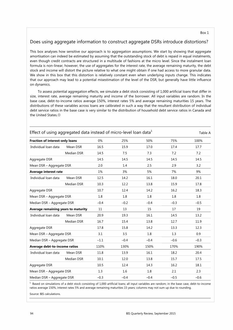
94 BIS Quarterly Review, September 2015
Box 1
Does using aggregate information to construct aggregate DSRs introduce distortions?
This box analyses how sensitive our approach is to aggregation assumptions. We start by showing that aggregate amortisation can indeed be estimated by assuming that the outstanding stock of debt is repaid in equal instalments, even though credit contracts are structured in a multitude of fashions at the micro level. Since the instalment loan formula is non-linear, however, the use of aggregates for the interest rate, the average remaining maturity, the debt stock and income will distort the picture relative to what one might obtain if one had access to more granular data. We show in this box that this distortion is relatively constant even when underlying inputs change. This indicates that our approach may lead to a potential misestimation of the level of the DSR, but generally have little influence on dynamics.
To assess potential aggregation effects, we simulate a debt stock consisting of 1,000 artificial loans that differ in size, interest rate, average remaining maturity and income of the borrower. All input variables are random. In the base case, debt-to-income ratios average 150%, interest rates 5% and average remaining maturities 15 years. The distributions of these variables across loans are calibrated in such a way that the resultant distribution of individual debt service ratios in the base case is very similar to the distribution of household debt service ratios in Canada and the United States.
Effect of using aggregated data instead of micro-level loan data1 Table A
Fraction of interest-only loans 0% 25% 50% 75% 100%
Individual loan data Mean DSR 16.5 15.9 17.0 17.4 17.7
Median DSR 14.5 7.5 7.3 7.2 7.2
Aggregate DSR 14.5 14.5 14.5 14.5 14.5
Mean DSR – Aggregate DSR 2.0 1.4 2.5 2.9 3.2
Average interest rate 1% 3% 5% 7% 9%
Individual loan data Mean DSR 12.5 14.2 16.1 18.0 20.1
Median DSR 10.3 12.2 13.8 15.9 17.8
Aggregate DSR 10.7 12.4 14.2 16.2 18.3
Mean DSR – Aggregate DSR 1.8 1.8 1.8 1.8 1.8
Median DSR – Aggregate DSR –0.4 –0.2 –0.4 –0.3 –0.5
Average remaining years to maturity 11 13 15 17 19
Individual loan data Mean DSR 20.9 19.3 16.1 14.5 13.2
Median DSR 16.7 15.4 13.8 12.7 11.9
Aggregate DSR 17.8 15.8 14.2 13.3 12.3
Mean DSR – Aggregate DSR 3.1 3.5 1.8 1.3 0.9
Median DSR – Aggregate DSR –1.1 –0.4 –0.4 –0.6 –0.3
Average debt-to-income ratios 110% 130% 150% 170% 190%
Individual loan data Mean DSR 11.8 13.9 16.1 18.2 20.4
Median DSR 10.1 12.0 13.8 15.7 17.5
Aggregate DSR 10.5 12.4 14.3 16.2 18.1
Mean DSR – Aggregate DSR 1.3 1.6 1.8 2.1 2.3
Median DSR – Aggregate DSR –0.3 –0.4 –0.4 –0.5 –0.61 Based on simulations of a debt stock consisting of 1,000 artificial loans; all input variables are random; in the base case, debt-to-income ratios average 150%, interest rates 5% and average remaining maturities 15 years; columns may not sum up due to rounding.
Source: BIS calculations.
BIS Quarterly Review, September 2015 95
The simulation highlights that, while our methodology produces an approximation error, this is little related to the instalment loan assumption. To check the validity of this assumption, we let the fraction of instalment loans vary between zero and 100%. The remaining loans in this case are interest-only loans, of which only 1/15 involve repaying the principal in each period, in line with an assumption that the average remaining maturity is 15 years. The upper panel of Table A shows the difference between using micro data and relying on aggregate data plus the instalment loan formula. On average, the two approaches differ by around 2.5 percentage points. But this difference varies only between 1.4 and 3.2 percentage points depending on our assumption about the share of interest-only loans. This variation is small, especially given that the composition of the loan portfolio is unlikely to change to such a degree within a particular country. As such, it indicates that the instalment loan assumption works well for constructing aggregate DSRs.
As discussed in the main text, while the main source of approximation error arises from the use of aggregate information, this more likely distorts the estimated mean of the DSR than its dynamics. In particular, the size and direction of this error remain fairly constant, as the overall levels of interest rates, debt-to-income ratios or maturities change. In the base case (average debt-to-income ratio = 150%, average interest rate = 5% and average remaining maturity = 15 years), the average DSR of the individual loans is 16.1%, which is 1.9 percentage points higher than the estimated DSR of 14.2%. If interest rates on average increase to 9%, the average DSR of individual loans rises to 20.1% and the estimated DSR rises to 18.3%, but the estimation error remains approximately the same, at 1.8 percentage points. Similar results emerge for changes in the average remaining maturity or debt-to-income ratios. Interestingly, the approximation error is even lower if we compare the estimated DSR with the median of the individual data. In any case, note that the ranges of the input parameters in this simulation are rather large. For instance, we simulate debt-to-income ratios from 110% to 190%, but it took around 20 years for the debt-to-income ratio for the total private sector in the United States to increase from 110% to 150%. Similarly, an increase in the average remaining maturity from 15 to 19 years (we simulate remaining maturities between 11 and 19 years) would require a doubling of the average remaining maturity on more than 25% of the outstanding loans, which is not likely to happen. The characteristics of the loan stock are thus likely to be relatively stable over time. This argues for the accuracy of the aggregate approach for estimating DSRs.
Based on the Consumer Expenditure Survey, Johnson and Li (2010) report the following distribution of household debt service burdens inthe United States from 1992 to 2004: 6% (20th percentile), 12% (40th percentile), 19% (60th percentile) and 28% (80th percentile). Calculating debt service burdens based on an instalment loan formula, the corresponding values in our sample are 2% (20th percentile), 10% (40th percentile), 17% (40th percentile) and 27% (80th percentile). The simulated distribution also broadly matches the distribution and main statistics of household DSRs in Canada from 1999 to 2000 (Faruqui (2008)). When checking the instalment loan assumption, we increased the sample size to 30,000, to avoid small-sample problems, when the fraction of interest-only loans that repay the principal is low. The median drops rapidly with the fraction of interest-only loans by construction, as 14/15 of the interest-only loans are not amortised at all.
For the household sector, we apply a constant 18-year average remaining maturity across countries and time. Two different approaches lead to this assumption. First, 18 years emerges as the average across countries, if we assume an average remaining maturity of 20 years for mortgages13 and six years for consumer loans,14 and weight these values by the respective share in households’
13 Mortgages are typically repaid over 25–30 years in advanced countries. In the simplest case, where the volume of loans taken out over consecutive years is always the same, the credit-weighted average remaining maturity across new and old (partially repaid) loans is between 16 and 19 years. If new borrowers take out larger nominal loans than old ones, which historically has happened, for instance, because of rising house prices, the weighted average remaining maturity of the stock of credit is higher, suggesting a figure of about 20 years. This is closely in line with the average remaining maturity of 21 years in the United States that has prevailed since the early 1990s, as shown by the biannual American Housing Survey (see http://www.census.gov/programs-surveys/ahs/data.html).
14 An average remaining maturity of six years for consumer loans provides the best fit when trying to replicate the Fed’s DSR for consumer loans. This is also consistent with the weighted average

96 BIS Quarterly Review, September 2015
Cross-country comparisons of interest rates and maturities Graph 2
Difference between average interest rates and bank lending rates, by sector
Maturity for the household sector1 Maturity for the private non-financial corporate sector4
From 1999 to latest; in % points Years Years
AU = Australia; BE = Belgium; CA = Canada; DE = Germany; ES = Spain; FI = Finland; FR = France; GB = United Kingdom; IT = Italy; KR = Korea; NL = Netherlands; PT = Portugal; SE = Sweden.
1 Includes Belgium, Finland, France, Germany, Italy, the Netherlands, Portugal, Spain and the United States. 2 Distribution of weighted average remaining maturities across countries, assuming that mortgages have an average remaining maturity of 20 years and consumer loans an average of six years. 3 Distribution of weighted average remaining maturities across countries based on information from initial contractual maturities in three broad buckets, assuming that 90% of the loans with short-term maturities and 75% of the loans with medium-term maturities get rolled over. 4 Distribution of weighted average remaining maturities across countries based on information from initial contractual maturities in three broad buckets. Includes Belgium, Denmark, Finland, France, Germany, Italy, the Netherlands, Portugal and Spain. 5 Rollovers: 90% short-term, 75% medium-term and 10% long-term.
Sources: ECB; national data; BIS calculations.
total debt (Graph 2, centre panel). Alternatively, for some countries, we have information on the amount of household loans on banks’ balance sheets grouped into three broad buckets of initial contractual maturities.15 Taking a weighted average across maturity buckets leads again to an average remaining maturity for household loans of around 18 years in all countries (Graph 2, centre panel). Interestingly, in both cases the variation across countries is small, supporting the use of a constant average maturity across countries. This simplifies the approach, and in any event using country-specific remaining maturities that vary from 16 to 19 years would not alter the DSRs significantly.
For the non-financial corporate sector, we apply a 13-year average remaining maturity. This value is more judgmental than in the case of the household sector, because we have little information on actual amortisations. However, we know that refinancing to extend maturity is very important. For instance, around 45% of bonds
remaining maturity of 6.5 years for consumer loans in the United States that has prevailed since 1980.
15 The three buckets are loans with initial contractual maturities of less than one year, between one and five years and above five years. We then assume that these buckets correspond to remaining maturities of one, three and 20 years, respectively. We also assume that 90% of the loans with short maturities and 75% of the loans in the middle bucket get rolled over (Box 2 discusses how rollovers affect remaining maturities). Dropping the rollover assumption shortens the average remaining maturities to 17.2 years and increases the cross-country variation somewhat.
–3.0
–1.5
0.0
1.5
3.0
AUBE CADE ES FI FRGB IT KR NL PT SE
Non-fin corporations:
House-holds:
Average5th–95th percentile
15
16
17
18
19
Consumer and Initial contractualmortgage loans2 maturities3
AverageAcross the country sample:
Min-max range
4
6
8
10
12
No rollovers Rollovers5
AverageAcross the country sample:
Min-max range
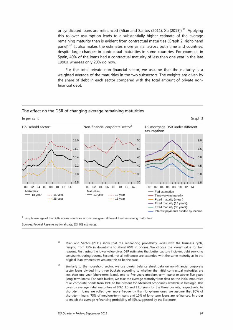
BIS Quarterly Review, September 2015 97
or syndicated loans are refinanced (Mian and Santos (2011), Xu (2015)).16 Applying this rollover assumption leads to a substantially higher estimate of the average remaining maturity than is evident from contractual maturities (Graph 2, right-hand panel).17 It also makes the estimates more similar across both time and countries, despite large changes in contractual maturities in some countries. For example, in Spain, 40% of the loans had a contractual maturity of less than one year in the late 1990s, whereas only 20% do now.
For the total private non-financial sector, we assume that the maturity is a weighted average of the maturities in the two subsectors. The weights are given by the share of debt in each sector compared with the total amount of private non-financial debt.
The effect on the DSR of changing average remaining maturities
In per cent Graph 3
Household sector1 Non-financial corporate sector1 US mortgage DSR under different assumptions
1 Simple average of the DSRs across countries across time given different fixed remaining maturities.
Sources: Federal Reserve; national data; BIS; BIS estimates.
16 Mian and Santos (2011) show that the refinancing probability varies with the business cycle, ranging from 45% in downturns to about 60% in booms. We choose the lowest value for two reasons. First, using the lower value gives DSR estimates that better capture incipient debt servicing constraints during booms. Second, not all refinances are extended with the same maturity as in the original loan, whereas we assume this to be the case.
17 Similarly to the household sector, we use banks’ balance sheet data on non-financial corporate sector loans divided into three buckets according to whether the initial contractual maturities are less than one year (short-term loans), one to five years (medium-term loans) or above five years (long-term loans). For each bucket, we take the average maturity from data on the initial maturities of all corporate bonds from 1990 to the present for advanced economies available in Dealogic. This gives us average initial maturities of 0.92, 3.5 and 13.3 years for the three buckets, respectively. As short-term loans are rolled over more frequently than long-term ones, we assume that 90% of short-term loans, 75% of medium-term loans and 10% of long-term loans are refinanced, in order to match the average refinancing probability of 45% suggested by the literature.
6.5
7.8
9.1
10.4
11.7
13.0
00 02 04 06 08 10 12 14
18-yearMaturities:
15-year25-year
30
35
40
45
50
55
00 02 04 06 08 10 12 14
13-yearMaturities:
10-year16-year
1.5
3.0
4.5
6.0
7.5
9.0
00 02 04 06 08 10 12 14
Fed estimationTime-varying maturityFixed maturity (mean)Fixed maturity (15 years)Fixed maturity (30 years)Interest payments divided by income

98 BIS Quarterly Review, September 2015
Box 2
Derivation of the DSR formula
In this box, we derive the instalment loan formula. We also show how we derive remaining maturities from contractual maturities.
To understand the instalment loan formula, consider a loan of size D with a per-period interest rate of i and a maturity of s periods. Let Dt denote the remaining principal in period t, with D=D1. Suppose that the per-period debt costs, Rt, are paid in equal portions over the maturity of the loan, ie R=R2=⋯=Rs, which means that the loan is structured as a so called instalment loan. How large is the debt cost, R, given D, i and s?
To derive a formula for R, consider what we know about debt costs in each period. In the first period, for instance, the payment must satisfy R=iD+D-D2 and in the t:th period R=iDt+Dt-D(t+1). In the last period, s, the payment satisfies iDs+Ds-D(s+1), but since there is no remaining principal in period s+1, ie D(s+1)=0, we have:
= 1 +This expression can then be used to derive the payment in the second-to-last payment period, which gives: = 1 + +(1 + ) = (1 + (1 + ))(1 + )Continuing recursively in this fashion until the first payment period, we get: = (∑ (1 + ) )(1 + )
which, using the formula for a finite geometric sum, becomes: = 1 − (1 + )−(1 + )
Solving for R gives: = −(1 + )1 − (1 + ) = −(1 + )−(1 + ) (1 − 1(1 + ) ) = 1 − (1 + )
Defining the debt service ratio as DSR=R/Y, where Y denotes income, we have the desired formula: = (1 − (1 + ) Given that borrowers can roll over debt with some probability, how can we estimate maturities from
information on initial contractual maturities? Consider a portfolio of loans with a contractual maturity of c periods. At maturity, each loan has a probability ρ of getting renewed for another c periods. Then, the maturity, s, of the portfolio satisfies:
= (1 − ) + (1 − )2 + (1 − )2 + ⋯ = (1 − ) (1 + 2 + 3 +⋯) = (1 − ) ( + 1)
and using the formula for the infinite sum of an arithmetico-geometric sequence gives:
= (1 − ) 11 − + (1 − ) = (1 − )Hence, the remaining contractual maturity can be simply calculated by dividing the contractual maturity by one
minus the rollover probability.
Even if our estimates for remaining maturities are inaccurate, this will mainly affect the level rather than the dynamics of DSRs. The solid lines in the left-hand and centre panels of Graph 3 show the average sectoral DSRs across countries,
BIS Quarterly Review, September 2015 99
using the baseline assumption of 18 and 13 years for the household sector and the non-financial corporate sector, respectively. The dotted lines show DSRs under alternative maturity assumptions. As can be seen from the graph, changes in the assumptions about remaining maturities have a first-order impact on the level but not on the dynamics of the estimated DSRs for both sectors. When we apply a higher maturity, the DSR naturally moves down since the loans are amortised over a longer period of time, while the opposite is true for lower maturities.
Keeping remaining maturities fixed across time and across countries is appealing because of its simplicity, but it may distort our estimates somewhat, beyond shifts in the level. Yet, as long as the structure does not change significantly and permanently, deviations are likely to be small and temporary. This can be illustrated for the US mortgage sector, where we have information on actual remaining maturities and the Federal Reserve’s own estimate of the mortgage debt service ratio as a reference point. Using time-varying average remaining maturities allows us to replicate the Fed’s estimates (black and red lines, right-hand panel of Graph 3).18 If we hold remaining maturities constant at their historical mean instead (yellow line), we overestimate the increase in the mortgage DSR around the financial crisis, as in fact average remaining maturities in that period rose from 21 to 24 years and then fell back. However, despite a substantial shift in remaining maturities, the difference between the DSRs based on time-varying and constant maturities is less than half a percentage point at any given point.19 The level shift from applying “wrong” remaining maturities is clearly visible in the graph. For instance, the dynamics of the debt service ratio are essentially unaffected whether we assume a remaining maturity of 15 years (purple line) or 30 years (green line).
The US example highlights again that it is important to take amortisations into account when assessing debt-related payments for households and firms. Mortgage interest payments alone relative to income (blue line) looked sustainable compared with historical levels, even at the height of the crisis.20 But once one accounts for amortisation, debt service ratios were substantially higher than in earlier periods or several years after the crisis.
The evolution of DSRs over the last 15 years
In this section, we use the BIS estimates to study the evolution of the DSR in different countries over the last 15 years. Given the difficulties in pinpointing the level accurately, it is more meaningful to compare national DSRs relative to their means rather than comparing their absolute levels. In a cross-country context, such
18 When constructing this estimate, we follow the Fed and assume a minimum repayment of 2% in each quarter for revolving consumer loans (ie 98% can be rolled over) and an average remaining maturity of other consumer loans of four years, in line with initial contractual maturities of five to six years, as observed for cars or student loans in the United States.
19 Given the inherent non-linearity in the instalment loan formula, a three-year shift in aggregate remaining maturities – for example, from 10 to 13 years – would have had a proportionally bigger impact.
20 Note that, while relatively small changes in the assumption about remaining maturity do not meaningfully affect the overall trend, extreme maturity assumptions would matter: for example, assuming a remaining maturity of 100 years would be misleading, as repayments in this case would be so low that the DSR and the ratio of interest payments to income would coincide.
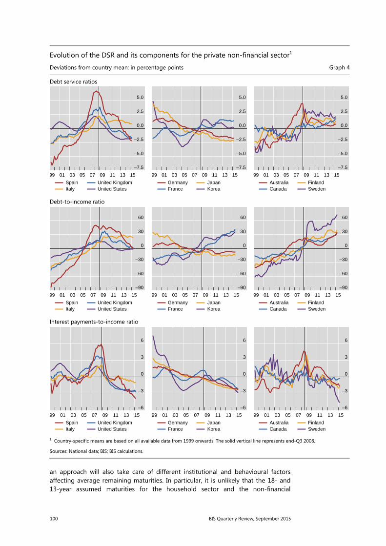
100 BIS Quarterly Review, September 2015
Evolution of the DSR and its components for the private non-financial sector1
Deviations from country mean; in percentage points Graph 4
Debt service ratios
Debt-to-income ratio
Interest payments-to-income ratio
1 Country-specific means are based on all available data from 1999 onwards. The solid vertical line represents end-Q3 2008.
Sources: National data; BIS; BIS calculations.
an approach will also take care of different institutional and behavioural factors affecting average remaining maturities. In particular, it is unlikely that the 18- and 13-year assumed maturities for the household sector and the non-financial
–7.5
–5.0
–2.5
0.0
2.5
5.0
99 01 03 05 07 09 11 13 15
SpainItaly
United KingdomUnited States
–7.5
–5.0
–2.5
0.0
2.5
5.0
99 01 03 05 07 09 11 13 15
GermanyFrance
JapanKorea
–7.5
–5.0
–2.5
0.0
2.5
5.0
99 01 03 05 07 09 11 13 15
AustraliaCanada
FinlandSweden
–90
–60
–30
0
30
60
99 01 03 05 07 09 11 13 15
SpainItaly
United KingdomUnited States
–90
–60
–30
0
30
60
99 01 03 05 07 09 11 13 15
GermanyFrance
JapanKorea
–90
–60
–30
0
30
60
99 01 03 05 07 09 11 13 15
AustraliaCanada
FinlandSweden
–6
–3
0
3
6
99 01 03 05 07 09 11 13 15
SpainItaly
United KingdomUnited States
–6
–3
0
3
6
99 01 03 05 07 09 11 13 15
GermanyFrance
JapanKorea
–6
–3
0
3
6
99 01 03 05 07 09 11 13 15
AustraliaCanada
FinlandSweden

BIS Quarterly Review, September 2015 101
corporate sector, respectively, will be fully accurate for all countries. Given that, as already discussed, average remaining maturities mainly affect the level and not the dynamics of the DSR, removing cross-country specific means allows for a more appropriate cross-country comparison of how DSRs have evolved over time.
Graph 4 illustrates how the DSR provides a more comprehensive assessment of debt burdens than the debt-to-income ratio or simple measures of interest payments relative to income, because it takes both interest payments and amortisations into account. This is clearly visible in the case of France or Korea. Debt-to-income ratios have been rising in both countries since the early 2000s (Graph 4, centre panels). At the same time, interest rates – and with them interest payments-to-income ratios – have followed a downward trend (Graph 4, bottom panels), allowing households and firms to carry larger amounts of debt with the same amount of income. In the case of Korea, the DSR for the total private non-financial sector has been fluctuating around a broadly stable trend. For France, on the other hand, the increase in debt-to-income ratios has outweighed the fall in interest rates, leading to an overall rise in the DSR (Graph 4, top centre panel).
Evolution of the DSR for the household and non-financial corporate sector1
Deviations from country mean; in percentage points Graph 5
Household sector
Non-financial corporate sector
1 Country-specific means are based on all available data from 1999 onwards. The solid vertical line represents end-Q3 2008.
Sources: National data; BIS; BIS calculations.
–4
–2
0
2
99 01 03 05 07 09 11 13 15
SpainItaly
United KingdomUnited States
–4
–2
0
2
99 01 03 05 07 09 11 13 15
GermanyFrance
JapanKorea
–4
–2
0
2
99 01 03 05 07 09 11 13 15
AustraliaCanada
FinlandSweden
–20
–10
0
10
20
99 01 03 05 07 09 11 13 15
SpainItaly
United KingdomUnited States
–20
–10
0
10
20
99 01 03 05 07 09 11 13 15
GermanyFrance
JapanKorea
–20
–10
0
10
20
99 01 03 05 07 09 11 13 15
AustraliaCanada
FinlandSweden
102 BIS Quarterly Review, September 2015
As such, DSRs provide an explanation for the limited amount of deleveraging that has taken place since the financial crisis, as documented by Buttiglione et al (2015), among others. Whereas debt-to-income ratios have been slow to fall, DSRs have dropped substantially in countries such as Spain, the United Kingdom and the United States (Graph 4, top left-hand panel), mainly due to the reduction in interest rates. Nonetheless, debt service ratios took several years to return to normal levels, helping to explain the weak post-crisis recovery (Juselius and Drehmann (2015)). DSRs are now below their sample average in many countries. Together with exceptionally low interest rates, this may reduce the incentives for further deleveraging.
DSRs can also provide a gauge of the sustainability of credit developments. For example, in Spain, the United Kingdom and the United States, household DSRs increased substantially ahead of the financial crisis (Graph 5, top left-hand panel). In Spain and the United Kingdom, this was accompanied by growing non-financial corporate DSRs (Graph 5, bottom left-hand panel). These developments are typical ahead of financial crisis. Indeed a rapid rise in DSRs has been found empirically to be a strong early warning indicator of systemic banking crises (Drehmann and Juselius (2014)).
At present, DSRs point to lower debt service burdens in some countries and sectors, but a substantial increase in others. For instance, non-financial corporate sector DSRs have been rising in Finland and Sweden, reaching high levels in comparison with cross-country benchmarks (Graph 5, bottom right-hand panel).
Conclusion
This special feature provides an introduction to the new BIS database on aggregate debt service ratios. The database currently covers DSRs for the total private non-financial sector for 32 countries, as well as DSRs for the household and the non-financial corporate sectors separately for 17 countries.
From a methodological perspective, the main contribution of the article is to show that it is possible to construct consistent and meaningful DSRs for a large set of countries with a relatively sparse set of aggregate data. Whilst the use of more granular data may result in different estimates for DSR levels, our methodology captures the dynamics of DSRs over time quite well. For practical purposes, the difficulties in pinpointing the DSR level imply that it is most meaningful to compare our estimates of the DSR over time, and to remove country-specific means.
Looking forward, efforts are under way to increase the time and country coverage of the database. This will allow users a broader historical and global perspective, which is important given the pivotal role of debt service burdens as a link between business and financial cycles.

BIS Quarterly Review, September 2015 103
References
Alessi, L, A Antunes, J Babecký, S Baltussen, M Behn, D Bonfim and D Zigraiová (2014): “Comparing different early warning systems: results from a horse race competition among members of the macro-prudential research network”, paper presented at the final conference of the Macroprudential Research Network.
Buttiglione, L, P Lane, L Reichlin and V Reinhart (2014): “Deleveraging? What deleveraging?”, Geneva Reports on the World Economy.
Dembiermont, C, M Drehmann and S Muksakunratana (2013): “How much does the private sector really borrow – a new database for total credit to the private non-financial sector”, BIS Quarterly Review, March, pp 65–81.
Drehmann, M and M Juselius (2012): “Do debt service costs affect macroeconomic and financial stability?”, BIS Quarterly Review, September, pp 21–34.
——— (2014): “Evaluating early warning indicators of banking crises: satisfying policy requirements”, International Journal of Forecasting, vol 30(3), pp 759–80.
Dynan, K, K Johnson and K Pence (2003): “Recent changes to a measure of US household debt service”, Federal Reserve Bulletin, vol 89(10), pp 417–26.
Faruqui, U (2008): “Indebtedness and the household financial health: an examination of the Canadian debt service ratio distribution”, Bank of Canada, Working Papers, no 46, December.
Federal Reserve Board (2013): “Household debt service and financial obligations ratios. About the release”, December.
Johnson, K and G Li (2010): “The debt-payment-to-income ratio as an indicator of borrowing constraints: evidence from two household surveys”, Journal of Money, Credit, and Banking, vol 42(7), pp 1373–90.
Juselius, M and M Drehmann (2015): “Leverage dynamics and the real burden of debt”, BIS Working Papers, no 501, May.
Mian, A and J Santos (2011): “Liquidity risk, maturity management and the business cycle”, mimeo.
Xu, Q (2015): “Kicking maturity down the road: early refinancing and maturity management in the corporate bond market”, University of Chicago Booth School of Business, job market paper.

BIS Quarterly Review, September 2015 105
Boris Hofmann
Előd Takáts
International monetary spillovers1
Interest rates have moved closely together internationally in recent years, despite business cycles often being at different stages across countries. We investigate whether international monetary spillovers drove this co-movement, ie whether interest rates in core advanced economies drove interest rates elsewhere. Applying a fixed-effects panel regression to 30 emerging market and smaller open advanced economies over the post-2000 period, we find that (i) US short- and long-term interest rates significantly affect the corresponding rates in other economies and (ii) these price spillovers reflect in part policy spillovers, ie that US policy rates affect policy rates in other countries. These monetary spillovers imply that the interest rate declines seen over the last seven years in the United States have had a considerable impact on interest rates elsewhere.
JEL classification: F33, F36, F42, F65.
Interest rates in core advanced economies, such as the United States, and those of emerging market economies (EMEs) and of smaller advanced economies move closely together, even though the business cycle has often been at different stages in these economies. For instance, as monetary policy eased in the United States in the wake of the Great Financial Crisis of 2007–09, short- and long-term interest rates also fell in countries not directly affected by it. And in May 2013, EME bond yields spiked in unison when the Federal Reserve signalled its intention to taper (ie scale down) its bond purchases. What drives this apparent correlation? Does it arise from synchronised business cycles or from other common factors that naturally drive interest rates in the same direction? Or, alternatively, does it reflect monetary spillovers, ie a direct impact of US interest rates on rates elsewhere, above and beyond what might be expected from other economic linkages?
To date, the evidence has been mixed. While most agree that there are significant spillovers in long-term interest rates, the evidence for short-term interest rates is less clear. For instance, Obstfeld (2015) finds that there are significant interest rate spillovers in long-term rates, but not in short-term rates.2 In contrast, Gray (2013), Edwards (2015) and Takáts and Vela (2014) report evidence of significant spillovers in policy rates.
1 The views expressed are those of the authors and do not necessarily reflect those of the BIS. We thank Claudio Borio, Ben Cohen, Dietrich Domanski, Hyun Song Shin and Christian Upper for helpful comments, and Emese Kuruc for excellent research assistance.
2 Turner (2014), Turner and Sobrun (2015) and Miyajima et al (2014) also confirm strong correlations and potential spillovers via long-term rates. He and McCauley (2013) highlight the role of dollar-denominated credit as a source of spillovers. Chen et al (2015) also find significant spillovers, but they document substantial heterogeneity in these effects among EMEs.

106 BIS Quarterly Review, September 2015
In our empirical approach, we use standard panel regressions to analyse monetary spillovers, which we define as spillovers in short- and long term rates, and in policy rates. In all our specifications, we explicitly control for the impact of domestic and global macroeconomic factors, and for global financial factors that might drive the raw (unconditional) interest rate correlations. Our sample covers 22 EMEs and eight smaller advanced economies.3 We focus on the period ranging from 2000 to 2014 and, in order to match financial and macroeconomic time series, we use quarterly data.
Our analysis differs from previous work primarily by focusing on economies that are well integrated in the global financial system and on the post-2000 period. Most previous studies included periphery countries that were only weakly integrated in the global economy and covered a longer period (starting in the early 1990s or even the 1980s). This difference in sample selection turns out to be important, because global financial and economic integration is a key driver of monetary spillovers. It determines the strength of investor arbitrage by tying bond market rates to those prevailing in the core economies. It also affects the degree to which policymakers might be concerned about capital flows and exchange rate volatility – concerns that would induce them to factor US interest rates into their monetary policy decisions. Hence, as countries differ substantially in how well integrated they are in the global economy, it is crucial to focus on the better integrated ones.4 Similarly, as economic and financial integration has significantly strengthened since the late 1990s,5 the subsequent period is the most relevant for our analysis. Incidentally, this time period also has the advantage for our analysis of not having been affected by major EME crises. The exclusion of such crises helps with econometric identification, as periods of stress were usually associated with strong idiosyncratic policy and interest rate movements, ie with large outliers in the data.
Our results provide new insights. We find economically and statistically significant spillovers from the United States to EMEs and smaller advanced economies. These spillovers are present not only in short- and long-term interest rates but also in policy rates.6 In other words, we find that interest rates in the United States affect interest rates elsewhere beyond what similarities in business cycles or global risk factors would justify. We also find that monetary spillovers take place under both fixed and floating exchange rate regimes, which lends some
3 The EMEs covered by our analysis are Brazil, Chile, China, Chinese Taipei, Colombia, the Czech Republic, Hong Kong SAR, Hungary, India, Indonesia, Israel, Korea, Malaysia, Mexico, Peru, the Philippines, Poland, Russia, Singapore, South Africa, Thailand and Turkey. The smaller advanced economies sample comprises Australia, Canada, Denmark, New Zealand, Norway, Sweden, Switzerland and the United Kingdom. Importantly, we do not include countries from the euro area, the other large currency zone.
4 For instance, taken together, the EMEs included in our country sample represent more than 95% of the weights of the JPMorgan Government Bond-Emerging Market Index (GBI-EM), a key local currency EME government bond index.
5 Specifically, the international investment position of all countries has increased, from below 100% of global GDP in 2000 to above 150% by 2013. Over the same period, world trade, measured as the average of export and imports, rose from below 20% to around 25% of global GDP.
6 We also conducted the analysis using country-dependent base currencies, specifically using the euro area as the base currency area for European EMEs and smaller advanced economies and the United States for the remaining countries. The results turned out to be very similar to the ones with the United States as the general base country. They are available upon request.
BIS Quarterly Review, September 2015 107
support to the conjecture in Rey (2013, 2014) that the global financial cycle constrains monetary policy irrespective of the exchange rate regime.7
From a policy perspective, our findings suggest that neither are interest rates fully independent nor is monetary policy fully unconstrained when economies and financial markets are closely integrated. Even under flexible exchange rates, central banks – though technically able – seem to find it difficult to conduct a monetary policy that is based purely on domestic factors and which ignores monetary developments in core advanced economies. Furthermore, our findings also shed some light on the causes of the persistently low interest rates that have prevailed globally over the past seven years. Back-of-the-envelope calculations based on our results suggest that easy monetary conditions in the United States have exerted considerable downward pressure on interest rates elsewhere.
The remainder of the feature is organised as follows. Section 1 documents the (unconditional) correlations between US rates and those in EMEs and smaller advanced economies. Section 2 analyses price spillovers in short- and long-term interest rates, and Section 3 looks at spillovers in policy rates. Section 4 discusses the economic size of spillovers, and Section 5 concludes.
Interest rate correlations
Interest rates in EMEs and smaller advanced economies tend to move closely together with the rates prevailing in core advanced economies, such as the United States (Graph 1). The co-movement is closest for long-term interest rates (Graph 1, left-hand panel). And, though less pronounced, it is also present for short-term interest rates (Graph 1, centre panel) and policy rates (Graph 1, right-hand panel). While EME rates (yellow line) tend to be higher than small advanced economy rates (blue line), both tend to move in the same direction as US rates (red line). The average correlation of the levels of long-term rates in EMEs and smaller advanced economies with those of US long-term rates at a quarterly frequency is 71%. The average correlation of short-term rates is 61% while that of policy rates is 63%.8
These correlations may reflect common economic and financial factors driving interest rates in a similar direction. For instance, shifts in international investors’ willingness to take risks could move monetary conditions in a similar direction globally. And the evolution of the US business cycle is likely to directly affect global macroeconomic conditions via trade channels – implying global monetary responses that are similar to those in the United States.
But alongside these channels, the observed interest rate correlations could also reflect genuine monetary spillovers. This could work through two channels. First, investor behaviour could tie interest rates together. Global investor portfolio reallocations might link the long-term rates of EMEs and smaller advanced
7 Specifically, Rey (2013, 2014) suggests that the global financial cycle has turned the classical “trilemma” of international macroeconomics into a “dilemma”. Instead of a free capital account and an independent monetary policy being feasible only under flexible exchange rates (“trilemma”), an independent monetary policy and a free capital account would be incompatible under any exchange rate regime (“dilemma”).
8 Average correlations are calculated for the period Q1 2000 to Q4 2014 for our country sample as listed in footnote 3 and Annex Table A1.

108 BIS Quarterly Review, September 2015
economies to those of the core financial centres. Investors searching for yield might shift funds from low-yielding bonds in the core economies to higher-yielding bonds elsewhere, pushing those yields down. Similarly, cross-border bank flows motivated by search-for-yield considerations might give rise to spillovers in interbank rates.
Second, monetary policies in EMEs and smaller advanced economies might follow those in the United States; in other words, there might be policy spillovers. For instance, central banks might want to prevent the emergence of large interest rate differentials to avoid exchange rate appreciation, which could result in a loss of trade competitiveness. Alternatively, they might be concerned that large interest rate differentials could induce speculative short-term capital inflows that could lead, in turn, to financial stability risks. In both cases, monetary authorities would aim to avoid large interest rate differentials against the rates prevailing in the United States. This would tie their policy rates to US policy rates, and, if market expectations then projected this linkage through the rest of the yield curve, other short- and long-term interest rates would follow.
By themselves, the high observed correlations between interest rates do not necessarily imply that price or policy spillovers are in operation. In order to identify such spillovers, one needs to estimate the correlations that remain after controlling for the other potential economic and financial drivers of domestic interest rates – in technical terms, to go from unconditional to conditional correlations.
Interest rates are closely correlated internationally
In per cent Graph 1
Long-term sovereign yield Short-term money market rate Policy rate1
1 For the United States, effective federal funds rate. 2 Median across Australia, Canada, Denmark, New Zealand, Norway, Sweden, Switzerland and the United Kingdom. 3 Median across Brazil, Chile, China, Chinese Taipei, Colombia, the Czech Republic, Hong Kong SAR,Hungary, India, Indonesia, Israel, Korea, Malaysia, Mexico, Peru, the Philippines, Poland, Russia, Singapore, South Africa, Thailand andTurkey, where data are available.
Sources: Federal Reserve Bank of St Louis, FRED; IMF, International Financial Statistics; Bloomberg; CEIC; Datastream; GFDatabase; national data; BIS calculations.
2
4
6
8
0
2
4
6
00 02 04 06 08 10 12 14
United States (rhs)
0
4
8
12
0
2
4
6
00 02 04 06 08 10 12 14
Other advanced economies2 (rhs)
0
4
8
12
0
2
4
6
00 02 04 06 08 10 12 14
Emerging market economies3 (lhs)

BIS Quarterly Review, September 2015 109
Spillovers in short- and long-term interest rates
We assess monetary spillovers in short- and long-term interest rates following Obstfeld (2015) by estimating the interest rate equation9 below in a panel fixed-effects setup:
∆ = + ∆ + ∆ + + 1 + 2 + (1)
where ∆ denotes the quarter-on-quarter change in the domestic interest rate and ∆ the quarter-on-quarter-change in the US interest rate. For short- and long-term interest rates, we consider the three-month interbank rate and the 10-year government bond yield, respectively.10 Our assumption is that US interest rates can influence interest rates elsewhere for the reasons discussed in the previous section, but not vice versa.11
By including the interaction of the change in the US interest rates with a dummy variable for pegged exchange rates, we can assess whether exchange rate flexibility enhances a country’s monetary independence. Specifically, is adummy variable that takes a value of one for a country that pegs its exchange rate to the US dollar in a given quarter and zero otherwise. We follow Obstfeld (2015) and use a de facto exchange rate classification scheme, coding a country as a “pegger” if its exchange rate has moved within a +/–2% range against the US dollar for at least eight quarters.12
The remaining regressors included in equation (1) control for factors that could drive unconditional interest rate correlations. Among them, dlogVIX denotes the log change of the VIX, the widely used measure of stock market volatility, and controls for the impact of changes in international investor sentiment as a potential common financial factor.13 is a vector of domestic macroeconomic variables: year-on-year inflation and real GDP growth which capture country-specific business cycle
9 The equation can be derived from the uncovered interest rate parity condition as shown in Obstfeld (2015).
10 Short-term rates are proxied by money market rates when interbank data are not available. Furthermore, short-term rates reflect shorter maturities for Russia (31–90 days) and Chile (30–89 days). Long-term yields reflect yields of seven- to 11-year bonds in Brazil and of nine-year bonds in Chile.
11 US short-term rates have been at near zero levels since 2009. This raises the question of how the inclusion of these observations affects our results. It turns out that estimating the spillover equations using data up to Q4 2008 yields results that are very similar to those obtained over the full sample.
12 The results do not change materially if we use a softer definition of a peg with a wider fluctuation range of +/–5%.
13 The VIX itself might of course be influenced by changes in US interest rates; see eg Rey (2013, 2014) and Bruno and Shin (2015). By controlling for the effect of the VIX on foreign interest rates, we isolate the interest rate spillovers that are additional to those of the VIX.
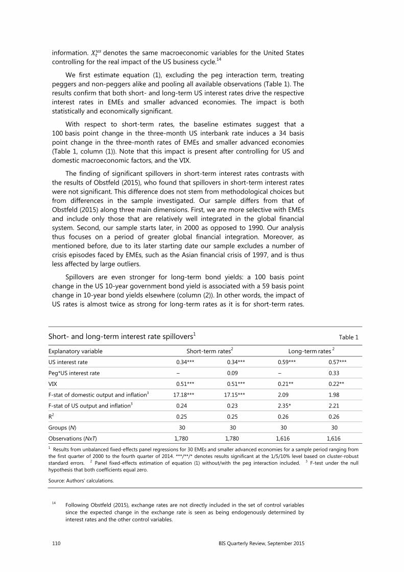
110 BIS Quarterly Review, September 2015
information. denotes the same macroeconomic variables for the United States controlling for the real impact of the US business cycle.14
We first estimate equation (1), excluding the peg interaction term, treating peggers and non-peggers alike and pooling all available observations (Table 1). The results confirm that both short- and long-term US interest rates drive the respective interest rates in EMEs and smaller advanced economies. The impact is both statistically and economically significant.
With respect to short-term rates, the baseline estimates suggest that a 100 basis point change in the three-month US interbank rate induces a 34 basis point change in the three-month rates of EMEs and smaller advanced economies (Table 1, column (1)). Note that this impact is present after controlling for US and domestic macroeconomic factors, and the VIX.
The finding of significant spillovers in short-term interest rates contrasts with the results of Obstfeld (2015), who found that spillovers in short-term interest rates were not significant. This difference does not stem from methodological choices but from differences in the sample investigated. Our sample differs from that of Obstfeld (2015) along three main dimensions. First, we are more selective with EMEs and include only those that are relatively well integrated in the global financial system. Second, our sample starts later, in 2000 as opposed to 1990. Our analysis thus focuses on a period of greater global financial integration. Moreover, as mentioned before, due to its later starting date our sample excludes a number of crisis episodes faced by EMEs, such as the Asian financial crisis of 1997, and is thus less affected by large outliers.
Spillovers are even stronger for long-term bond yields: a 100 basis point change in the US 10-year government bond yield is associated with a 59 basis point change in 10-year bond yields elsewhere (column (2)). In other words, the impact of US rates is almost twice as strong for long-term rates as it is for short-term rates.
14 Following Obstfeld (2015), exchange rates are not directly included in the set of control variables since the expected change in the exchange rate is seen as being endogenously determined by interest rates and the other control variables.
Short- and long-term interest rate spillovers1 Table 1
Explanatory variable Short-term rates2 Long-term rates 2
US interest rate 0.34*** 0.34*** 0.59*** 0.57***
Peg*US interest rate – 0.09 – 0.33
VIX 0.51*** 0.51*** 0.21** 0.22**
F-stat of domestic output and inflation3 17.18*** 17.15*** 2.09 1.98
F-stat of US output and inflation3 0.24 0.23 2.35* 2.21
R2 0.25 0.25 0.26 0.26
Groups (N) 30 30 30 30
Observations (NxT) 1,780 1,780 1,616 1,616 1 Results from unbalanced fixed-effects panel regressions for 30 EMEs and smaller advanced economies for a sample period ranging from the first quarter of 2000 to the fourth quarter of 2014. ***/**/* denotes results significant at the 1/5/10% level based on cluster-robust standard errors. 2 Panel fixed-effects estimation of equation (1) without/with the peg interaction included. 3 F-test under the null hypothesis that both coefficients equal zero.
Source: Authors’ calculations.
BIS Quarterly Review, September 2015 111
This result confirms previous research, including Obstfeld (2015), that found significant long-term interest rate spillovers. It should be noted that for both our study and the research conducted by Obstfeld (2015), outliers related to the 1990s EME crises are less relevant for the estimations of long-term rates, since bond yields for many EMEs are available only from the early 2000s onwards.
The economic and statistical significance of interest rate spillovers does not critically depend on whether the exchange rate is pegged. The peg interaction term remains insignificant if we include it in equation (1), both for short- and for long-term rates, implying that the spillover estimates for peggers and non-peggers do not differ in a statistically significant way from each other (columns (2) and (4)). Furthermore, the size and significance of the baseline coefficient for the US interest rate are not affected by the inclusion of the interaction term. This finding provides some empirical support for Rey’s (2013, 2014) conjecture that, in practice, exchange rate flexibility might not shield countries from external monetary spillovers.
The results also highlight the role of investor risk aversion, as proxied by the VIX. The VIX materially affects short- and long-term interest rates even aftercontrolling for other factors (third row, Table 1). Higher risk aversion is associated with an increase in short- and long-term interest rates in EMEs and smaller advanced economies. This is consistent with the oft described impact of increased risk aversion: short- and long-term interest rates rise as investors retreat, capital flows ebb and exchange rates come under downward pressure. As discussed above (footnote 13), changes in US interest rates also influence investor risk sentiment, so that the estimated effect of the VIX on interest rates abroad also reflects in part indirect interest rate spillovers.
Domestic macroeconomic variables also affect short-term interest rates in a significant way. Technically, the F-tests strongly reject the null hypothesis that the coefficients on domestic growth and inflation are zero for short-term interest rates (fourth row, Table 1). Long-term interest rates are, however, not significantly affected by domestic macroeconomic factors.
Finally, the US business cycle is not a statistically significant driver of short- and long-term interest rates, ie the F-tests cannot reject the null hypothesis that the coefficients on the US macroeconomic variables are zero (fifth row, Table 1). This also indicates that the identified price spillovers do not result from an indirect impact of the US business cycle, beyond the impact exerted through US short-and long-term rates.
Policy rate spillovers
The significant price spillovers in three-month interbank rates are indicative of policy spillovers, since short-term interbank rates are usually closely linked to policy rates. However, there is scope for focusing directly on policy rates rather than interbank rates: interbank rates diverged from policy rates in parts of the sample period, specifically in periods of financial distress, which could have influenced the
112 BIS Quarterly Review, September 2015
results. Furthermore, and more generally, one needs to investigate policy rate spillovers explicitly to address the policy questions raised in the previous literature.15
To assess policy rate spillovers, we apply three different empirical setups that reflect the various approaches to the analysis of policy rate setting used in the literature.
First, we estimate equation (1) with ∆ as the quarter-on-quarter change in the domestic policy rate and ∆ as the quarter-on-quarter-change in the effective federal funds rate. All the other variables are defined as before. This is basically a straightforward extension of the previous section’s analysis of spillovers in market interest rates to changes in policy rates.
Second, we estimate a standard positive, or descriptive, interest rate rule in the level of policy rates, augmented to include the US policy rate to test for the presence of spillovers. Formally, we estimate the following equation in a panel fixed-effects regression:
= + + + + + 1 + 2 + (2)
where is the policy rate, is the effective federal funds rate and logVIX denotes the natural logarithm of the VIX. includes the domestic output gap16 and inflation, while includes year-on-year inflation and real GDP growth for the United States, included again to control for the impact of the US business cycle. As in equation (1), we check whether there is a difference in policy spillovers between peggers and non-peggers by interacting the federal funds rate with the peg-dummy variable.17
Third, we investigate the extent to which deviations from a normative Taylor rule (Taylor (1993)) can be explained by the US policy rate – controlling for other
15 Here, policy spillovers are understood in a behavioural sense, ie they arise from the reaction of monetary authorities in recipient countries (say, out of concerns about the impact of external developments on exchange rates and capital flows). While we focus on spillovers in policy rates, in a broader sense, they have also occurred through long-term interest rates via large-scale asset purchases and forward guidance. These unconventional policies have increasingly driven long-term rates in core financial centres since the onset of the Great Financial Crisis and have influenced long-term rates elsewhere through the long-term rate spillovers documented in Table 1.
16 Output gap estimates are calculated from quarterly data using the standard Hodrick-Prescott (HP) filter with a smoothing parameter of 1,600.
17 The inclusion of a lagged dependent variable, which is standard in the literature for capturing interest rate smoothing by central banks, can give rise to biases in our panel estimation. First, Nickell (1981) has shown that dynamic panels with small time series dimensions are biased, with the size of the bias depending inversely on the size of the time series sample. Second, fixed-effects estimators of dynamic panels can be biased if there is heterogeneity in the slope coefficients across countries (Pesaran and Smith (1995)). In our application, these biases are, however, likely to be small. The time series dimension of the panel model is relatively large, which should mitigate the Nickell bias. At the same time, the coefficient of the lagged endogenous variable (ie the degree of interest rate smoothing) is fairly homogenous across countries and not very far from one (the panel coefficient estimate is 0.83), which should mitigate the heterogeneity bias. Excluding the lagged dependent variable from equation (2) could help avoid these biases in the panel estimation, but this might in turn give rise to omitted variable biases since the other variables might proxy for the omitted lagged domestic interest rate.
BIS Quarterly Review, September 2015 113
potential drivers.18 This approach is particularly relevant since persistent deviations of policy rates from levels implied by normative Taylor rules have emerged over the past couple of years and international policy spillovers have been identified as one potential driving force for this phenomenon (Hofmann and Bogdanova (2012)). Formally, we estimate the following equation in a panel fixed-effects regression:
− = + + + + + (3)
where is the policy rate implied by a normative Taylor rule, while all other variables are defined as in equation (2). The Taylor rates are calculated for each country as i = r*+π* + 1.5(π–π*) + 0.5y, where π is a measure of inflation, y is a measure of the output gap, π* is the inflation target and r* is the long-run real interest rate, here proxied by real trend output growth. π* is set equal to the official inflation target/objective, and otherwise to the sample average or trend inflation estimated through a standard Hodrick-Prescott (HP) filter. The Taylor rates are calculated for each country for all combinations of four measures of inflation and three measures of the output gap to obtain a range and an average of possible Taylor rates.
The results show economically and statistically significant spillovers from policy rates in the United States to those in EMEs and smaller advanced economies across all specifications (Table 2).19 The specification of policy rate changes suggest that a 100 basis point change in the federal funds rate is associated with a 26 basis point shift in the policy rate of EMEs and smaller advanced economies (column (1)), which is slightly smaller than the impact we found for changes in three-month interbank rates. In the descriptive interest rate rule, the estimated impact is somewhat larger, at 46 basis points (column (3)).20 The result is basically the same for the normative Taylor rule, with a 100 basis point change in the federal funds rate being associated with a 43 basis point shift in the policy rate of EMEs and smaller advanced economies (column (5)).
Consistent with our findings in the previous section, we find only weak evidence that exchange rate flexibility might strengthen monetary policy autonomy. The estimated coefficients for the pegger interaction term are statistically significant only at the 10% level in the estimations of the deviations from the normative Taylor rule, while they are insignificant in the two other estimations (second row, Table 2).
Global risk aversion, as proxied by the VIX, significantly affects policy rate setting even after controlling for US interest rates, US domestic macroeconomic
18 The Taylor (1993) rule is a simple monetary policy rule mechanically linking the level of the policy rate to deviations of inflation from its target and of output from its potential (the output gap) through fixed reaction coefficients. While it was initially proposed as a simple illustration for the United States of desirable policy rules that had emerged from the academic literature at that time, it has become a popular normative benchmark against which to assess the monetary policy stance also in EMEs and smaller advanced economies.
19 In order to assess the impact of the near zero policy rate period since 2009, we also re-estimated the policy spillover equations using data up to Q4 2008 only and found the results again to be very similar to those obtained over the full sample.
20 The long-run impact is given by /(1 − ). When equation (3) is estimated without the lagged domestic interest rate, the estimated impact of the US policy rate is somewhat larger, at 0.7 (BIS (2015)), potentially reflecting omitted variable bias as indicated in footnote 17.
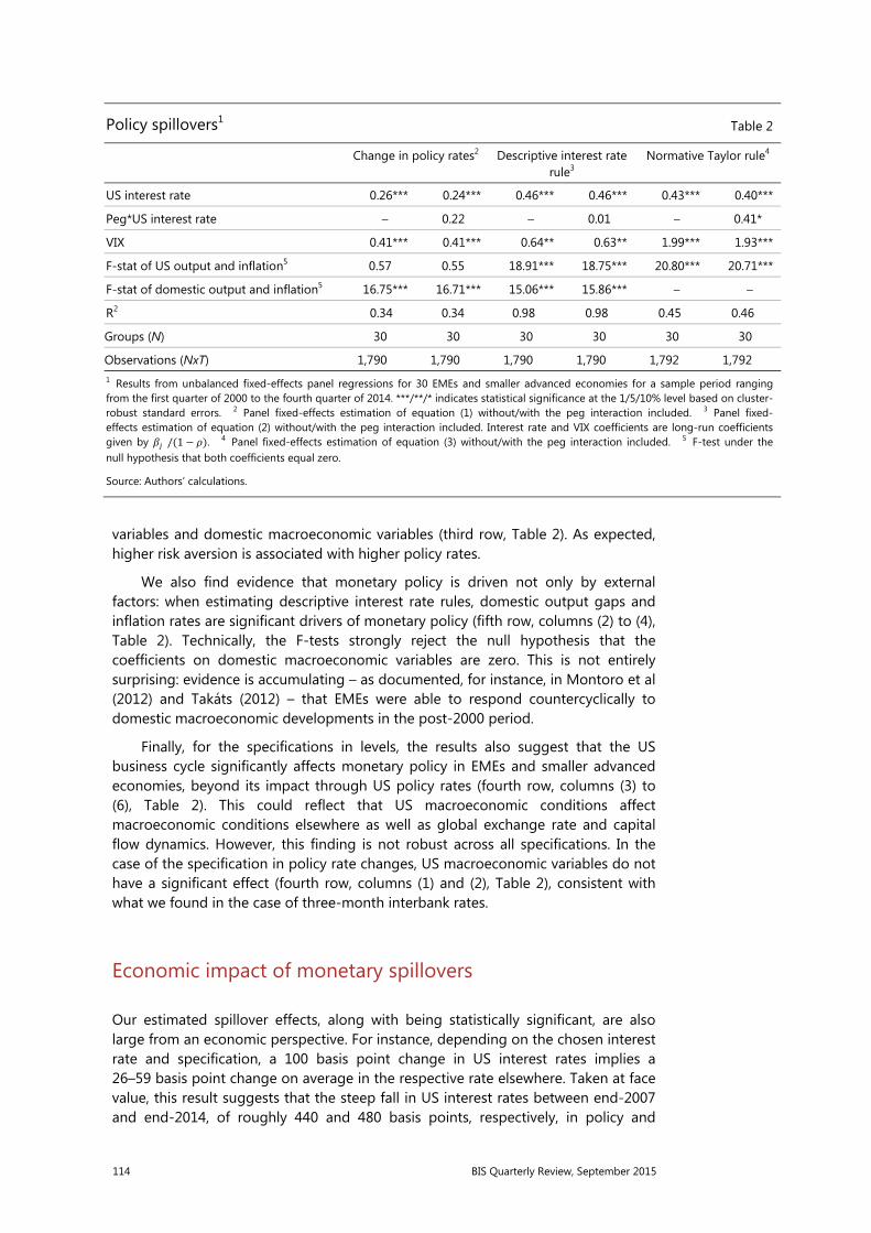
114 BIS Quarterly Review, September 2015
variables and domestic macroeconomic variables (third row, Table 2). As expected, higher risk aversion is associated with higher policy rates.
We also find evidence that monetary policy is driven not only by external factors: when estimating descriptive interest rate rules, domestic output gaps and inflation rates are significant drivers of monetary policy (fifth row, columns (2) to (4), Table 2). Technically, the F-tests strongly reject the null hypothesis that the coefficients on domestic macroeconomic variables are zero. This is not entirely surprising: evidence is accumulating – as documented, for instance, in Montoro et al (2012) and Takáts (2012) – that EMEs were able to respond countercyclically to domestic macroeconomic developments in the post-2000 period.
Finally, for the specifications in levels, the results also suggest that the US business cycle significantly affects monetary policy in EMEs and smaller advanced economies, beyond its impact through US policy rates (fourth row, columns (3) to (6), Table 2). This could reflect that US macroeconomic conditions affect macroeconomic conditions elsewhere as well as global exchange rate and capital flow dynamics. However, this finding is not robust across all specifications. In the case of the specification in policy rate changes, US macroeconomic variables do not have a significant effect (fourth row, columns (1) and (2), Table 2), consistent with what we found in the case of three-month interbank rates.
Economic impact of monetary spillovers
Our estimated spillover effects, along with being statistically significant, are also large from an economic perspective. For instance, depending on the chosen interest rate and specification, a 100 basis point change in US interest rates implies a 26–59 basis point change on average in the respective rate elsewhere. Taken at face value, this result suggests that the steep fall in US interest rates between end-2007 and end-2014, of roughly 440 and 480 basis points, respectively, in policy and
Policy spillovers1 Table 2
Change in policy rates2 Descriptive interest rate
rule3 Normative Taylor rule4
US interest rate 0.26*** 0.24*** 0.46*** 0.46*** 0.43*** 0.40***
Peg*US interest rate – 0.22 – 0.01 – 0.41*
VIX 0.41*** 0.41*** 0.64** 0.63** 1.99*** 1.93***
F-stat of US output and inflation5 0.57 0.55 18.91*** 18.75*** 20.80*** 20.71***
F-stat of domestic output and inflation5 16.75*** 16.71*** 15.06*** 15.86*** – –
R2 0.34 0.34 0.98 0.98 0.45 0.46
Groups (N) 30 30 30 30 30 30
Observations (NxT) 1,790 1,790 1,790 1,790 1,792 1,792 1 Results from unbalanced fixed-effects panel regressions for 30 EMEs and smaller advanced economies for a sample period ranging from the first quarter of 2000 to the fourth quarter of 2014. ***/**/* indicates statistical significance at the 1/5/10% level based on cluster-robust standard errors. 2 Panel fixed-effects estimation of equation (1) without/with the peg interaction included. 3 Panel fixed-effects estimation of equation (2) without/with the peg interaction included. Interest rate and VIX coefficients are long-run coefficients given by /(1 − ). 4 Panel fixed-effects estimation of equation (3) without/with the peg interaction included. 5 F-test under the null hypothesis that both coefficients equal zero.
Source: Authors’ calculations.
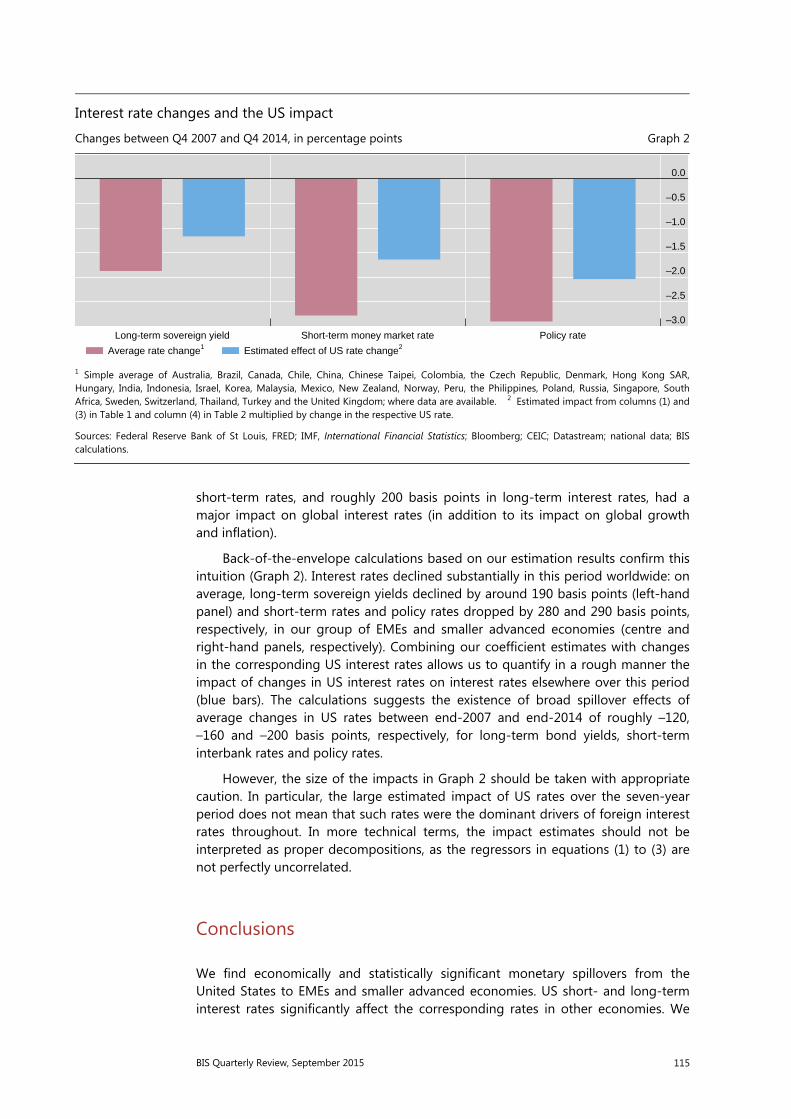
BIS Quarterly Review, September 2015 115
short-term rates, and roughly 200 basis points in long-term interest rates, had a major impact on global interest rates (in addition to its impact on global growth and inflation).
Back-of-the-envelope calculations based on our estimation results confirm this intuition (Graph 2). Interest rates declined substantially in this period worldwide: on average, long-term sovereign yields declined by around 190 basis points (left-hand panel) and short-term rates and policy rates dropped by 280 and 290 basis points, respectively, in our group of EMEs and smaller advanced economies (centre and right-hand panels, respectively). Combining our coefficient estimates with changes in the corresponding US interest rates allows us to quantify in a rough manner the impact of changes in US interest rates on interest rates elsewhere over this period (blue bars). The calculations suggests the existence of broad spillover effects of average changes in US rates between end-2007 and end-2014 of roughly –120, –160 and –200 basis points, respectively, for long-term bond yields, short-terminterbank rates and policy rates.
However, the size of the impacts in Graph 2 should be taken with appropriate caution. In particular, the large estimated impact of US rates over the seven-year period does not mean that such rates were the dominant drivers of foreign interest rates throughout. In more technical terms, the impact estimates should not be interpreted as proper decompositions, as the regressors in equations (1) to (3) are not perfectly uncorrelated.
Conclusions
We find economically and statistically significant monetary spillovers from the United States to EMEs and smaller advanced economies. US short- and long-term interest rates significantly affect the corresponding rates in other economies. We
Interest rate changes and the US impact
Changes between Q4 2007 and Q4 2014, in percentage points Graph 2
1 Simple average of Australia, Brazil, Canada, Chile, China, Chinese Taipei, Colombia, the Czech Republic, Denmark, Hong Kong SAR, Hungary, India, Indonesia, Israel, Korea, Malaysia, Mexico, New Zealand, Norway, Peru, the Philippines, Poland, Russia, Singapore, South Africa, Sweden, Switzerland, Thailand, Turkey and the United Kingdom; where data are available. 2 Estimated impact from columns (1) and (3) in Table 1 and column (4) in Table 2 multiplied by change in the respective US rate.
Sources: Federal Reserve Bank of St Louis, FRED; IMF, International Financial Statistics; Bloomberg; CEIC; Datastream; national data; BIS calculations.
–3.0
–2.5
–2.0
–1.5
–1.0
–0.5
0.0
Long-term sovereign yield Short-term money market rate Policy rate
Average rate change1 Estimated effect of US rate change2
116 BIS Quarterly Review, September 2015
further find that these spillovers reflect in part policy rate spillovers, ie that US policy rates affect policy rates in other countries. These results are obtained while controlling for US and domestic macroeconomic conditions and movements in the VIX. Thus, monetary conditions in the United States affect monetary conditionselsewhere beyond what similarities in business cycles or global risk factors would justify.
Our findings further suggest that in economies that are closely integrated in the global economy and global financial markets, financial conditions are not independent. Interest rates in the core financial centres are important driving factors. At the same time, monetary policy appears to be constrained. Even under flexible exchange rates, central banks seem to find it difficult to conduct a monetary policy that is based purely on domestic factors and that ignores monetary developments in core advanced economies – although they are technically capable of doing so. This probably reflects the trade-offs that central banks face: in internationally open economic and financial systems, large interest rate differentials, even if vindicated by domestic economic conditions, could still lead to excessive capital inflows or strong exchange rate appreciations – which could, in turn, pose risks to either financial stability or trade competitiveness.
Our findings also shed some light on the causes of persistently low global interest rates over the past seven years. Back-of-the-envelope calculations suggest that easy monetary conditions in the United States have significantly lowered interest rates elsewhere. This finding supports the notion that global monetary spillovers have been an important factor behind persistently low global interest rates.
The policy question going forward is whether non-US central banks will follow US monetary policy as the Federal Reserve starts to raise the policy rate. Our results suggest that spillovers are present when the Fed tightens, which is supported by the fact that our sample period includes the Fed’s tightening cycle of 2004–06. Yet, some caution is warranted. It might well be that spillovers are not fully symmetrical: for instance, policymakers might tolerate exchange rate depreciations or short-term capital outflows better than appreciations and inflows. Or they might be even more sensitive about them. Hence, while our results provide evidence on past spillovers, one should be cautious in applying them to predict potential future spillovers.
BIS Quarterly Review, September 2015 117
References
Bank for International Settlements (2015): 85th Annual Report, June, Table V.C, p 91.
Bruno, V and H S Shin (2015): “Capital flows and the risk-taking channel of monetary policy”, Journal of Monetary Economics, vol 71, pp 119–32.
Chen, Q, A Filardo, D He and F Zhu (2015): “Financial crisis, US unconventional monetary policy and international spillovers”, BIS Working Papers, no 494, March.
Edwards, S (2015): “Monetary policy independence under flexible exchange rates: an illusion?”, The World Economy, vol 38(5), May, pp 773–87.
Gray, C (2013): ”Responding to a monetary superpower: investigating the behavioral spillovers of US monetary policy”, Atlantic Economic Journal, vol 41(2), June, pp 173–84.
He, D and R McCauley (2013): “Transmitting global liquidity to East Asia: policy rates, bond yields, currencies and dollar credit”, BIS Working Papers, no 431, October.
Hofmann, B and B Bogdanova (2012): “Taylor rules and monetary policy: a global ‘Great Deviation’?”, BIS Quarterly Review, September, pp 37–49.
Miyajima, K, M Mohanty and J Yetman (2014): “Spillovers of US unconventional monetary policy to Asia: the role of long-term interest rates”, BIS Working Papers, no 478, December.
Montoro, C, E Takáts and J Yetman (2012): “Is monetary policy constrained by fiscal policy?”, BIS Papers, no 67, October, pp 11–30.
Nickell, S (1981): “Biases in dynamic models with fixed effects”, Econometrica, vol 49(6), pp 1417–26.
Obstfeld, M (2015): “Trilemmas and trade-offs: living with financial globalisation”, BIS Working Papers, no 480, January.
Pesaran, M and R Smith (1995): “Estimating long-run relationships from dynamic heterogeneous panels”, Journal of Econometrics, vol 68(1), pp 79–113.
Rey, H (2013): “Dilemma not trilemma: the global financial cycle and monetary policy independence”, paper presented at the 25th Federal Reserve Bank of Kansas City Annual Economic Policy Symposium, Jackson Hole, Wyoming, August.
——— (2014): “The international credit channel and monetary autonomy”, Mundell-Fleming Lecture, IMF, 13 November.
Takáts, E (2012): “Countercyclical policies in emerging markets”, BIS Quarterly Review, June, pp 25–31.
Takáts, E and A Vela (2014): “International monetary policy transmission”, BIS Papers, no 78, August, pp 25–44.
Taylor, J (1993): “Discretion versus policy rules in practice”, Carnegie-Rochester Series on Public Policy, no 39, pp 195–214.
Turner, P (2014): “The global long-term interest rate, financial risks and policy choices in EMEs”, BIS Working Papers, no 441, February.
Turner, P and J Sobrun (2015): “Bond markets and monetary policy dilemmas for the emerging markets”, BIS Working Papers, no 508, August.
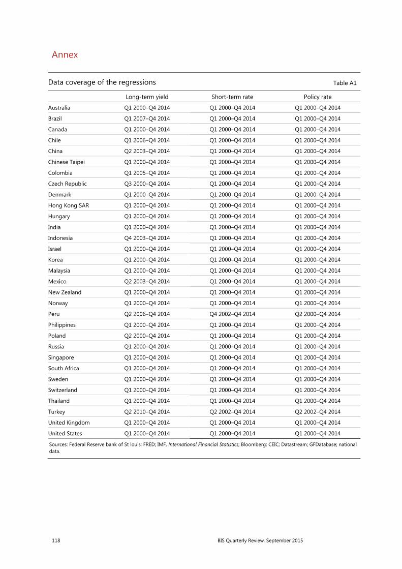
118 BIS Quarterly Review, September 2015
Annex
Data coverage of the regressions Table A1
Long-term yield Short-term rate Policy rate
Australia Q1 2000–Q4 2014 Q1 2000–Q4 2014 Q1 2000–Q4 2014
Brazil Q1 2007–Q4 2014 Q1 2000–Q4 2014 Q1 2000–Q4 2014
Canada Q1 2000–Q4 2014 Q1 2000–Q4 2014 Q1 2000–Q4 2014
Chile Q1 2006–Q4 2014 Q1 2000–Q4 2014 Q1 2000–Q4 2014
China Q2 2003–Q4 2014 Q1 2000–Q4 2014 Q1 2000–Q4 2014
Chinese Taipei Q1 2000–Q4 2014 Q1 2000–Q4 2014 Q1 2000–Q4 2014
Colombia Q1 2005–Q4 2014 Q1 2000–Q4 2014 Q1 2000–Q4 2014
Czech Republic Q3 2000–Q4 2014 Q1 2000–Q4 2014 Q1 2000–Q4 2014
Denmark Q1 2000–Q4 2014 Q1 2000–Q4 2014 Q1 2000–Q4 2014
Hong Kong SAR Q1 2000–Q4 2014 Q1 2000–Q4 2014 Q1 2000–Q4 2014
Hungary Q1 2000–Q4 2014 Q1 2000–Q4 2014 Q1 2000–Q4 2014
India Q1 2000–Q4 2014 Q1 2000–Q4 2014 Q1 2000–Q4 2014
Indonesia Q4 2003–Q4 2014 Q1 2000–Q4 2014 Q1 2000–Q4 2014
Israel Q1 2000–Q4 2014 Q1 2000–Q4 2014 Q1 2000–Q4 2014
Korea Q1 2000–Q4 2014 Q1 2000–Q4 2014 Q1 2000–Q4 2014
Malaysia Q1 2000–Q4 2014 Q1 2000–Q4 2014 Q1 2000–Q4 2014
Mexico Q2 2003–Q4 2014 Q1 2000–Q4 2014 Q1 2000–Q4 2014
New Zealand Q1 2000–Q4 2014 Q1 2000–Q4 2014 Q1 2000–Q4 2014
Norway Q1 2000–Q4 2014 Q1 2000–Q4 2014 Q1 2000–Q4 2014
Peru Q2 2006–Q4 2014 Q4 2002–Q4 2014 Q2 2000–Q4 2014
Philippines Q1 2000–Q4 2014 Q1 2000–Q4 2014 Q1 2000–Q4 2014
Poland Q2 2000–Q4 2014 Q1 2000–Q4 2014 Q1 2000–Q4 2014
Russia Q1 2000–Q4 2014 Q1 2000–Q4 2014 Q1 2000–Q4 2014
Singapore Q1 2000–Q4 2014 Q1 2000–Q4 2014 Q1 2000–Q4 2014
South Africa Q1 2000–Q4 2014 Q1 2000–Q4 2014 Q1 2000–Q4 2014
Sweden Q1 2000–Q4 2014 Q1 2000–Q4 2014 Q1 2000–Q4 2014
Switzerland Q1 2000–Q4 2014 Q1 2000–Q4 2014 Q1 2000–Q4 2014
Thailand Q1 2000–Q4 2014 Q1 2000–Q4 2014 Q1 2000–Q4 2014
Turkey Q2 2010–Q4 2014 Q2 2002–Q4 2014 Q2 2002–Q4 2014
United Kingdom Q1 2000–Q4 2014 Q1 2000–Q4 2014 Q1 2000–Q4 2014
United States Q1 2000–Q4 2014 Q1 2000–Q4 2014 Q1 2000–Q4 2014
Sources: Federal Reserve bank of St louis; FRED; IMF, International Financial Statistics; Bloomberg; CEIC; Datastream; GFDatabase; national data.

BIS Quarterly Review, September 2015 119
Eli Remolona
Ilhyock Shim
The rise of regional banking in Asia and the Pacific1
Cross-border banking activity within the Asia-Pacific region has intensified since the Great Financial Crisis of 2007−09. In the years leading up to the crisis, much of the cross-border activity in the region had been driven by dollar credit intermediated largely by European banks. In the wake of the crisis, this global intermediation lost much of its European leg. Banks from within the region stepped in and soon came to dominate cross-border activity. Adding impetus to the intraregional trend, the ASEAN member governments have adopted a regional banking integration framework. Mindful of the lessons of European banking integration, the banking authorities in the region are seeking to balance the efficiency gains of regional integration against the risks of financial instability.
JEL classification: F34, F36, G21.
Cross-border banking in Asia and the Pacific has steadily increased over the last dozen years, interrupted only by the Great Financial Crisis of 2007−09. This steady increase, however, masked a major change in the pattern of financial intermediation. In the global cross-border banking boom of 2001−07, most of the activity had taken the form of a flow of dollars from the United States to Europe and then to Asia-Pacific as well as back to the United States, with European banks serving as the major intermediaries (Avdjiev et al (2015)). Since the crisis, however, European banks have held back and banks from Asia-Pacific have stepped in, so that the bulk of the intermediation is now conducted within the region.
The intraregional trend seems likely to be sustained. Reinforcing this trend, member governments of the Association of Southeast Asian Nations (ASEAN) have recently adopted a regional banking integration framework. This will soon allow banks qualified in one member jurisdiction to operate freely in others. A rise of large regional banks could bring efficiency gains but could also enlarge channels of regional contagion.
In this article, we first characterise the regional dimensions of cross-border banking activity in Asia and the Pacific. We then analyse the proliferation of regional bank branches and subsidiaries in the region, how these units fund themselves, and what the implications are for their lending behaviour. Finally, we raise some specific financial stability issues: the potential for common and concentrated creditors as well as for systemic risks involving foreign branches; liquidity risks in foreign
1 We thank Stefan Avdjiev, Claudio Borio, Ben Cohen, Dietrich Domanski, Robert McCauley, Patrick McGuire, Hyun Song Shin, Chang Shu and Philip Wooldridge for helpful comments and suggestions. We also thank Jimmy Shek for excellent statistical assistance. The views expressed in this article are those of the authors and do not necessarily reflect those of the BIS.

120 BIS Quarterly Review, September 2015
currency funding; and the increasing share of short-term foreign currency loans in Asia-Pacific banks’ intraregional lending.
Trends in regional banking activity
Shifting patterns in global banking, especially the cross-border provision of dollar credit, have had an important bearing on banking flows in the Asia-Pacific region. In the period before the Great Financial Crisis, as Shin (2013) has shown, global banks increased leverage to provide cross-border dollar funding, and European banks played a prominent role in cross-border dollar intermediation. After the crisis, a prolonged period of low global long-term interest rates, new bank regulations and efforts to repair balance sheets led to a major shift in the pattern of cross-border financial intermediation. Global banks increasingly gave way to asset managers investing in long-term debt securities. This shift also opened up opportunities for Asia-Pacific banks to expand their activity within the region.
Strong growth and changing players
The last dozen years have seen a strong increase in cross-border banking in the Asia-Pacific region. Between 2002 and 2007, international bank claims on emerging Asia-Pacific almost quadrupled to $844 billion (Graph 1, left-hand panel). In 2007, euro area banks accounted for about a third of these claims, Asia-Pacific banks for a similar share, and Swiss, UK and US banks for roughly the other third. Over the same period, international bank claims on Latin America and the Caribbean grew more slowly, while those on emerging economies in Europe almost quintupled, albeit from a smaller base.2
The Great Financial Crisis was a watershed in international banking, and the Asia-Pacific region was no exception. Between 2007 and 2008, international lending in the region fell by $120 billion.3 But this halt was only temporary: international lending in Asia rebounded from 2009. International claims on the region more than doubled in five years (Graph 1, left-hand panel). China stands out, with cross-border claims on the country growing almost sixfold from 2008 to 2014 (Table 1). Hong Kong SAR and Singapore played an important role as regional banking centres, by intermediating a large amount of cross-border funds relative to GDP (Box 1).
The strong growth in international claims on emerging Asia-Pacific between 2009 and 2014 stands in contrast to developments elsewhere. During the same period, international claims on Latin America and the Caribbean grew by 48%, while those on emerging economies in Europe shrank by 11%. By March 2015, international bank claims on the emerging Asia-Pacific region totalled $1.9 trillion, while those on Latin America and the Caribbean and emerging economies in Europe stood at $624 billion and $597 billion, respectively.
2 International bank claims on Latin America and the Caribbean grew by 52% to reach $346 billion, while those on emerging economies in Europe grew by 388% to reach $792 billion.
3 It should be noted that the fluctuations reported here are not on an exchange rate-adjusted basis. This is particularly relevant for the change between 2007 and 2008.
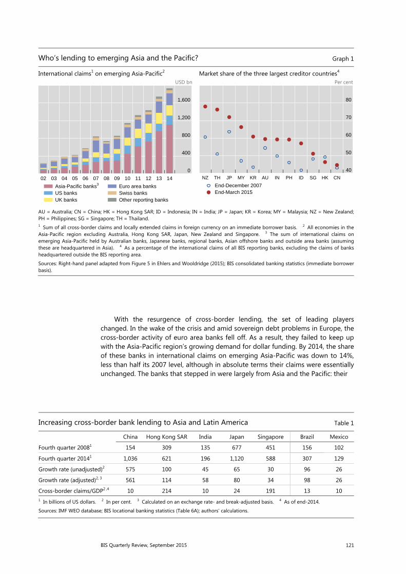
BIS Quarterly Review, September 2015 121
With the resurgence of cross-border lending, the set of leading players changed. In the wake of the crisis and amid sovereign debt problems in Europe, the cross-border activity of euro area banks fell off. As a result, they failed to keep up with the Asia-Pacific region’s growing demand for dollar funding. By 2014, the share of these banks in international claims on emerging Asia-Pacific was down to 14%, less than half its 2007 level, although in absolute terms their claims were essentially unchanged. The banks that stepped in were largely from Asia and the Pacific: their
Who’s lending to emerging Asia and the Pacific? Graph 1
International claims1 on emerging Asia-Pacific2 Market share of the three largest creditor countries4 USD bn Per cent
AU = Australia; CN = China; HK = Hong Kong SAR; ID = Indonesia; IN = India; JP = Japan; KR = Korea; MY = Malaysia; NZ = New Zealand; PH = Philippines; SG = Singapore; TH = Thailand. 1 Sum of all cross-border claims and locally extended claims in foreign currency on an immediate borrower basis. 2 All economies in the Asia-Pacific region excluding Australia, Hong Kong SAR, Japan, New Zealand and Singapore. 3 The sum of international claims on emerging Asia-Pacific held by Australian banks, Japanese banks, regional banks, Asian offshore banks and outside area banks (assumingthese are headquartered in Asia). 4 As a percentage of the international claims of all BIS reporting banks, excluding the claims of banks headquartered outside the BIS reporting area.
Sources: Right-hand panel adapted from Figure 5 in Ehlers and Wooldridge (2015); BIS consolidated banking statistics (immediate borrowerbasis).
Increasing cross-border bank lending to Asia and Latin America Table 1
China Hong Kong SAR India Japan Singapore Brazil Mexico
Fourth quarter 20081 154 309 135 677 451 156 102
Fourth quarter 20141 1,036 621 196 1,120 588 307 129
Growth rate (unadjusted)2 575 100 45 65 30 96 26
Growth rate (adjusted)2, 3 561 114 58 80 34 98 26
Cross-border claims/GDP2 ,4 10 214 10 24 191 13 10 1 In billions of US dollars. 2 In per cent. 3 Calculated on an exchange rate- and break-adjusted basis. 4 As of end-2014.
Sources: IMF WEO database; BIS locational banking statistics (Table 6A); authors’ calculations.
0
400
800
1,200
1,600
02 03 04 05 06 07 08 09 10 11 12 13 14
Asia-Pacific banks3
US banksUK banks
Euro area banksSwiss banksOther reporting banks
40
50
60
70
80
NZ TH JP MY KR AU IN PH ID SG HK CN
End-December 2007End-March 2015
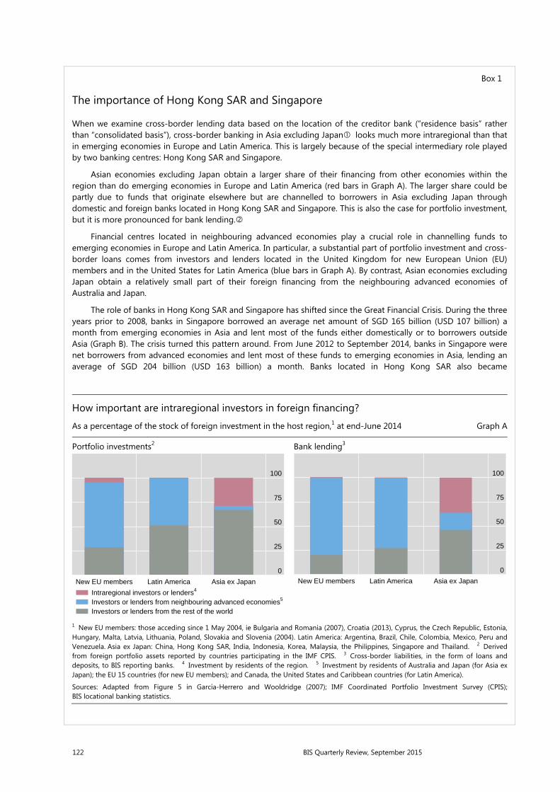
122 BIS Quarterly Review, September 2015
Box 1
The importance of Hong Kong SAR and Singapore
When we examine cross-border lending data based on the location of the creditor bank (“residence basis“ rather than “consolidated basis”), cross-border banking in Asia excluding Japan looks much more intraregional than that in emerging economies in Europe and Latin America. This is largely because of the special intermediary role played by two banking centres: Hong Kong SAR and Singapore.
Asian economies excluding Japan obtain a larger share of their financing from other economies within the region than do emerging economies in Europe and Latin America (red bars in Graph A). The larger share could be partly due to funds that originate elsewhere but are channelled to borrowers in Asia excluding Japan through domestic and foreign banks located in Hong Kong SAR and Singapore. This is also the case for portfolio investment, but it is more pronounced for bank lending.
Financial centres located in neighbouring advanced economies play a crucial role in channelling funds to emerging economies in Europe and Latin America. In particular, a substantial part of portfolio investment and cross-border loans comes from investors and lenders located in the United Kingdom for new European Union (EU) members and in the United States for Latin America (blue bars in Graph A). By contrast, Asian economies excluding Japan obtain a relatively small part of their foreign financing from the neighbouring advanced economies of Australia and Japan.
The role of banks in Hong Kong SAR and Singapore has shifted since the Great Financial Crisis. During the three years prior to 2008, banks in Singapore borrowed an average net amount of SGD 165 billion (USD 107 billion) a month from emerging economies in Asia and lent most of the funds either domestically or to borrowers outside Asia (Graph B). The crisis turned this pattern around. From June 2012 to September 2014, banks in Singapore were net borrowers from advanced economies and lent most of these funds to emerging economies in Asia, lending an average of SGD 204 billion (USD 163 billion) a month. Banks located in Hong Kong SAR also became
How important are intraregional investors in foreign financing?
As a percentage of the stock of foreign investment in the host region,1 at end-June 2014 Graph A
Portfolio investments2 Bank lending3
1 New EU members: those acceding since 1 May 2004, ie Bulgaria and Romania (2007), Croatia (2013), Cyprus, the Czech Republic, Estonia, Hungary, Malta, Latvia, Lithuania, Poland, Slovakia and Slovenia (2004). Latin America: Argentina, Brazil, Chile, Colombia, Mexico, Peru and Venezuela. Asia ex Japan: China, Hong Kong SAR, India, Indonesia, Korea, Malaysia, the Philippines, Singapore and Thailand. 2 Derived from foreign portfolio assets reported by countries participating in the IMF CPIS. 3 Cross-border liabilities, in the form of loans and deposits, to BIS reporting banks. 4 Investment by residents of the region. 5 Investment by residents of Australia and Japan (for Asia ex Japan); the EU 15 countries (for new EU members); and Canada, the United States and Caribbean countries (for Latin America).
Sources: Adapted from Figure 5 in García-Herrero and Wooldridge (2007); IMF Coordinated Portfolio Investment Survey (CPIS); BIS locational banking statistics.
0
25
50
75
100
New EU members Latin America Asia ex Japan
Intraregional investors or lenders4
Investors or lenders from neighbouring advanced economies5
Investors or lenders from the rest of the world
0
25
50
75
100
New EU members Latin America Asia ex Japan

BIS Quarterly Review, September 2015 123
The changing role of banks in Singapore
In billions of Singapore dollars Graph B
Pre-Lehman bankruptcy (June 2005–May 2008) Post-European debt crisis (June 2012–September 2014)
Sources: Monetary Authority of Singapore; authors’ calculations.
bigger net lenders in the emerging Asia-Pacific region (including Singapore) over this period, while reducing their net lending outside the region (Graph C).
The changing role of banks in Hong Kong SAR1
In billions of Hong Kong dollars Graph C
Pre-Lehman bankruptcy (Q2 2005–Q2 2008) Post-European debt crisis (Q2 2011–Q2 2014)
“Emerging Asia” includes all economies in the Asia-Pacific region except Australia, Japan and New Zealand, which are included in“Developed Asia”.1 Numbers are based on net external liabilities vis-à-vis non-residents.
Sources: Hong Kong Monetary Authority; authors’ calculations.
We compare three different emerging market regions: Asia, Europe and Latin America. For Asia-Pacific, we therefore focus on nine majoremerging economies and exclude Australia, Japan and New Zealand, as described in footnote 1 to Graph A. McCauley et al (2002) analyse bonds underwritten and loans syndicated for borrowers in Asia excluding Japan between 1999 and 2002, and find that Asian bond investors and banks on average committed half of the funds involved.

124 BIS Quarterly Review, September 2015
share went up from 31% in 2007 to 57% in 2014 (Graph 1, left-hand panel).4 As discussed below, the greater role of banks from within the region led to an even greater use of short-term lending than before.
The shift coincided with greater concentration in the creditor banking systems. Between the fourth quarter of 2007 and the first quarter of 2015, the combined market share of the three largest creditor countries rose for most of the major economies in the region (Graph 1, right-hand panel). The increase in concentration was pronounced for Indonesia, Korea, Malaysia, New Zealand, the Philippines and Thailand. For these six borrowing countries as a group, the five largest creditors in the first quarter of 2015 included three economies from the region – Australia, Japan and Singapore – besides the United Kingdom and the United States. In 2007, the list of the five largest creditors had included France and Germany instead of Australia and Singapore. As of the first quarter of 2015, Australia was the most important creditor for New Zealand, Japan for Indonesia and Thailand, and Singapore for Malaysia.
Regional banks’ foreign affiliates and business models
Foreign branches and subsidiaries
Cross-border banking involves either a bank in one country lending directly to borrowers in another, or a foreign bank lending through local branches or subsidiaries. To the extent that intraregional cross-border banking activity in Asia and the Pacific continues to intensify, the regional expansion of Asia-Pacific banks is likely to take the form of increased activity by branches and subsidiaries, as banks seek to establish a more permanent institutional presence in their target markets. Within the narrower ASEAN region, a recent banking integration initiative is likely to quicken the process (Box 2).
Almost all of the major economies in Asia-Pacific have banks with foreign branches or subsidiaries elsewhere in the region. As of the end of 2014, together the banks of Australia, China, India, Japan, Korea and Singapore counted 30 or more foreign branches and subsidiaries in the 12 major economies in the region. Most of them are also hosts to regional banks: China, Hong Kong SAR, Japan and Singapore each had 30 or more foreign branches and subsidiaries from elsewhere in the region (Graph 2).
In establishing a presence elsewhere in the region, Asia-Pacific banks tend to do so in the form of branches rather than subsidiaries: the former outnumber the latter by two to one. Foreign banks from outside the Asia-Pacific region also set up their local affiliates in the region predominantly in the form of branches: their Asia-Pacific branches outnumber their subsidiaries by five to one. However, banks
4 Among Asia-Pacific banks, lending by outside area banks (ie banks located in the BIS reporting area but headquartered outside) to emerging Asia-Pacific economies has increased sharply over the past decade, while Australian, Japanese and Singaporean banks have steadily increased lending to the region. McGuire and van Rixtel (2012) show that, even though the nationality of outside area banks is not known, data from BIS banking statistics and other sources indicate that the bulk of the increase in international claims extended by outside area banks is to borrowers in China, and is largely consistent with the increase in the total assets of Chinese banks’ foreign offices in Asia.
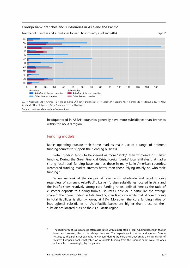
BIS Quarterly Review, September 2015 125
headquartered in ASEAN countries generally have more subsidiaries than branches within the ASEAN region.
Funding models
Banks operating outside their home markets make use of a range of different funding sources to support their lending business.
Retail funding tends to be viewed as more “sticky” than wholesale or market funding. During the Great Financial Crisis, foreign banks’ local affiliates that had a strong local retail funding base, such as those in many Latin American countries, weathered funding market stresses better than those relying mainly on wholesale funding.5
When we look at the degree of reliance on wholesale and retail funding regardless of currency, Asia-Pacific banks’ foreign subsidiaries located in Asia and the Pacific show relatively strong core funding ratios, defined here as the ratio of customer deposits to funding from all sources (Table 2). In particular, the average share of their core funding in total funding stands at 75%, while that of core funding in total liabilities is slightly lower, at 71%. Moreover, the core funding ratios of intraregional subsidiaries of Asia-Pacific banks are higher than those of their subsidiaries located outside the Asia-Pacific region.
5 The legal form of subsidiaries is often associated with a more stable retail funding base than that of branches. However, this is not always the case. The experience in central and eastern Europe testifies to this point. For example, in Hungary during the euro area debt crisis, the subsidiaries of western European banks that relied on wholesale funding from their parent banks were the ones vulnerable to deleveraging by the parents.
Foreign bank branches and subsidiaries in Asia and the Pacific
Number of branches and subsidiaries for each host country as of end-2014 Graph 2
AU = Australia; CN = China; HK = Hong Kong SAR; ID = Indonesia; IN = India; JP = Japan; KR = Korea; MY = Malaysia; NZ = NewZealand; PH = Philippines; SG = Singapore; TH = Thailand.
Sources: National data; authors’ calculations.
TH
SG
PH
NZ
MY
KR
JP
IN
ID
HK
CN
AU
0 10 20 30 40 50 60 70 80 90 100 110 120 130 140
Asia-Pacific home countriesOther home countries
Branches:Asia-Pacific home countriesOther home countries
Subsidiaries:

126 BIS Quarterly Review, September 2015
Another key aspect of business models is the funding currency. For foreign bank subsidiaries, local currency funding is generally more stable than funding in other currencies such as the US dollar. This is partly because local currency deposits mainly consist of relatively stable customer deposits for domestic use, while foreign currency deposits are made mainly by corporations or financial institutions that are sensitive to exchange rate and other developments. Lending by international banks’ foreign affiliates that are funded in local currency is considerably less volatile than cross-border lending (see Ehlers and Wooldridge (2015) and references therein).
In aggregate, banks headquartered in six Asia-Pacific economies rely on local currency funding for their lending to the region to almost the same degree as those headquartered elsewhere (Table 3). Local currency liabilities represented 27% of the intraregional assets of Asia-Pacific banks, compared with 26% for banks headquartered elsewhere. However, in many host countries, banks headquartered in Asia and the Pacific have a lower share of local currency liabilities than those headquartered elsewhere. In particular, Asia-Pacific banks in Australia, China, Chinese Taipei, Hong Kong SAR, India, Korea, the Philippines and Singapore all have a lower share of local currency liabilities than non-Asia-Pacific banks in the respective economies. By contrast, Asia-Pacific banks that lend to Indonesia, Japan, Malaysia, New Zealand and Thailand maintain higher levels of local currency funding than those headquartered in the Americas and Europe.
Another way to look at the funding model is in terms of the local currency funding gap, defined as the difference between local currency assets and local
Core funding ratios of foreign subsidiaries of Asia-Pacific banks1
In per cent, as of end-2013 Table 2
Ratio of core funding to total funding2 Ratio of core funding to total liabilities3
Subsidiaries in Asia-Pacific
Subsidiaries outside Asia-Pacific
Subsidiaries in Asia-Pacific
Subsidiaries outside Asia-Pacific
Australian banks 70 88 69 87
Chinese banks 74 75 68 54
Indian banks 96 67 94 66
Japanese banks 75 74 73 72
Korean banks 90 – 87 – Malaysian banks 89 – 85 – Singaporean banks 80 – 78 – Thai banks 79 – 76 – All banks 75 74 71 631 Based on a sample of 103 subsidiaries owned by 27 banks headquartered in eight Asia-Pacific economies. Sixty-four subsidiaries are located in the Asia-Pacific region, and the other 39 outside the region. In the sample, banks headquartered in Korea, Malaysia, Singapore and Thailand have no subsidiary located outside the Asia-Pacific region. 2 Total customer deposits (ie the sum of current, savings and term deposits) are used as a proxy for core funding. Total funding is the sum of total deposits, money market and short-term funding, total long-term funding, derivatives and trading liabilities. 3 Total liabilities are the sum of total funding (ie total interest bearing liabilities), fair value portion of debt, credit impairment reserves, reserves for pension and others, tax liabilities, other deferred liabilities, discontinued operations, insurance and other non-interest bearing liabilities.
Sources: Bankscope; authors’ calculations.
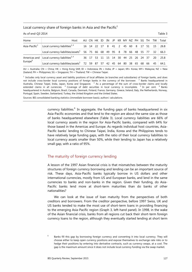
BIS Quarterly Review, September 2015 127
currency liabilities.6 In aggregate, the funding gaps of banks headquartered in six Asia-Pacific economies and that lend to the region are about the same size as those of banks headquartered elsewhere (Table 3). Local currency liabilities are 66% of local currency assets in the region for Asia-Pacific banks, compared with 64% for those based in the Americas and Europe. As regards individual host countries, Asia-Pacific banks’ lending to Chinese Taipei, India, Korea and the Philippines tends to have relatively large funding gaps, with the ratio of their local currency liabilities to local currency assets smaller than 50%, while their lending to Japan has a relatively small gap, with a ratio of 95%.
The maturity of foreign currency lending
A lesson of the 1997 Asian financial crisis is that mismatches between the maturity structures of foreign currency borrowing and lending can be an important source of risk. These days, Asia-Pacific banks typically borrow in US dollars and other international currencies, mostly from US and European banks, and lend in the same currencies to banks and non-banks in the region. Given their funding, do Asia-Pacific banks lend more at short-term maturities than do banks of other nationalities?
We can look at the issue of loan maturity from the perspectives of both creditors and borrowers. From the creditor perspective, before 1997 Swiss, UK and US banks tended to make the most use of short-term loans in providing financing to the emerging Asia-Pacific region (Graph 3, left-hand panel). In 1998, in the wake of the Asian financial crisis, banks from all regions cut back their short-term foreign currency loans to the region, although they eventually started lending at short term
6 Banks fill this gap by borrowing foreign currency and converting it into local currency. They will choose either to keep open currency positions and expose themselves to exchange rate risks or to hedge their positions by entering into derivative contracts, such as currency swaps, at a cost. The gap is the maximum amount since it does not include local currency funding via the swap market.
Local currency share of foreign banks in Asia and the Pacific1
As of end-Q3 2014 Table 3
Home Host AU CN HK ID IN JP KR MY NZ PH SG TH TW Total
Asia-Pacific2 Local currency liabilities3, 4 16 14 22 17 8 41 2 45 60 8 17 51 15 26.8
Local currency liabilities/assets5 56 75 66 68 49 95 8 78 66 48 55 77 32 66.3
Americas and Europe6
Local currency liabilities3, 4 36 17 53 11 15 14 30 44 25 26 24 37 20 25.8
Local currency liabilities/assets5 72 59 87 57 42 45 64 80 38 65 68 66 45 64.1
AU = Australia; CN = China; HK = Hong Kong SAR; ID = Indonesia; IN = India; JP = Japan; KR= Korea; MY= Malaysia; NZ = NewZealand; PH = Philippines; SG = Singapore; TH = Thailand; TW = Chinese Taipei.
1 Includes only local currency asset and liability positions of local affiliates (ie branches and subsidiaries) of foreign banks, and doesnot include cross-border local currency positions of foreign banks in the currency of the borrower. 2 Banks headquartered in Australia, Chinese Taipei, India, Japan, Korea and Singapore. 3 As a percentage of the sum of cross-border claims and locally extended claims in all currencies. 4 Coverage of debt securities in local currency is incomplete. 5 In per cent. 6 Banks headquartered in Austria, Belgium, Brazil, Canada, Denmark, Finland, France, Germany, Greece, Ireland, Italy, the Netherlands, Norway,Portugal, Spain, Sweden, Switzerland, Turkey, the United Kingdom and the United States.
Sources: BIS consolidated banking statistics (immediate borrower basis); authors’ calculations.

128 BIS Quarterly Review, September 2015
Box 2
ASEAN banking integration and lessons from Europe
The ASEAN Banking Integration Framework
The ASEAN Banking Integration Framework (ABIF) aims to achieve a free flow of financial services within the ASEAN regional banking market by 2020. Under the ABIF, member countries have adopted the scheme of Qualified ASEAN Banks (QABs), in which a bank qualified in one jurisdiction will receive equal treatment in the others. To recognise the different levels of readiness among members, the ABIF process specifies two stages: a multilateral stage and a bilateral one. The multilateral stage will establish ASEAN-wide guidelines, while the bilateral stage will involve negotiations between countries on the admission of QABs. The framework will be implemented at two speeds: first among the five larger ASEAN economies, and later including the others.
The larger ASEAN economies are moving forward in negotiating bilateral agreements. On 31 December 2014, Bank Indonesia, the Financial Services Authority of Indonesia and the Central Bank of Malaysia signed a bilateral agreement that outlined the measures the two countries would implement under the ABIF, set out the definition of QABs and identified the market access and operational flexibilities that QABs would enjoy. As bilateral negotiations proceed among ASEAN governments, the negotiations have become catalysts for enhancing bank supervision and regulation in individual member jurisdictions in anticipation of an increasingly integrated banking system in the region.
Some lessons from banking integration in Europe
In many respects, the ASEAN members are following in Europe’s footsteps. The member countries of the European Economic Area (EEA), consisting of the EU countries plus Iceland, Liechtenstein and Norway, agreed to mutual recognition of their supervisory frameworks in May 1992, and implemented in 1993 the “single passport” for banks, which ASEAN’s QABs scheme resembles closely. The single passport fostered banking integration in Europe, although this proceeded only gradually.
One lesson from banking integration in the EEA is that the single passport should have been accompanied by effective area-wide banking supervision. Restoring confidence in the European banking system after the Great Financial Crisis of 2007−09 and the subsequent European sovereign debt crisis has required extraordinary efforts by the authorities. These have included the establishment of a single supervisory mechanism in the euro area, a comprehensive review of the quality of major banks’ balance sheets, and macro stress tests to determine how much capital they would need to weather further adverse shocks. A related challenge currently being discussed is the setting of appropriate regulatory risk weights on credit to lower-rated EU sovereigns (Hannoun (2011)). Similar challenges are likely to arise as ASEAN financial authorities make progress in fully implementing QABs and seek to harmonise national regulations among the ASEAN members.
Another lesson is the importance of sound cross-border resolution frameworks. The resolution of troubled banks proved to be particularly difficult in the single banking market. For example, three Icelandic banks − Glitnir, Kaupthing Bank and Landsbanki − maintained large operations in the Netherlands and the United Kingdom under the EEA passport scheme. The collapse of these banks after 2008 sparked a cross-border dispute over who should pay for the bailout of their depositors. There was neither a region-wide resolution framework nor a bailout mechanism for dealing with failing cross-border banks. Progress has now been made with regard to resolving such issues in the future. A single rulebook for the resolution of banks and large investment firms in all EU member states came into force in January 2015. The new rules harmonised and improved the tools for dealing with failing banks across the European Union. At the same time, national resolution funds are being established. ASEAN members will be watching these steps closely as they work to develop their own resolution framework for regional banking integration.
ASEAN’s 10 member countries can be divided into the larger “ASEAN-5” economies (Indonesia, Malaysia, the Philippines, Singapore andThailand) and the smaller “BCLMV” economies (Brunei, Cambodia, Laos, Myanmar and Vietnam). For detailed accounts of the European lessons for ASEAN’s banking integration, see Volz (2013) and Elliott (2014).
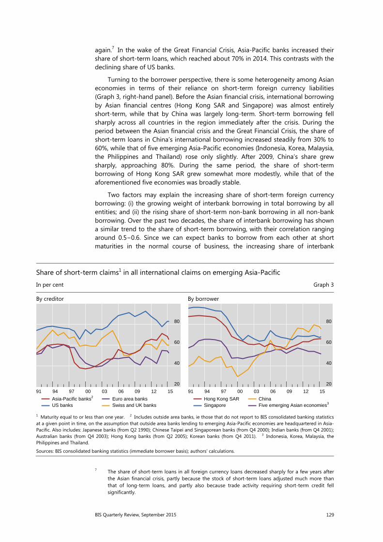
BIS Quarterly Review, September 2015 129
again.7 In the wake of the Great Financial Crisis, Asia-Pacific banks increased their share of short-term loans, which reached about 70% in 2014. This contrasts with the declining share of US banks.
Turning to the borrower perspective, there is some heterogeneity among Asian economies in terms of their reliance on short-term foreign currency liabilities (Graph 3, right-hand panel). Before the Asian financial crisis, international borrowing by Asian financial centres (Hong Kong SAR and Singapore) was almost entirely short-term, while that by China was largely long-term. Short-term borrowing fell sharply across all countries in the region immediately after the crisis. During the period between the Asian financial crisis and the Great Financial Crisis, the share of short-term loans in China’s international borrowing increased steadily from 30% to 60%, while that of five emerging Asia-Pacific economies (Indonesia, Korea, Malaysia, the Philippines and Thailand) rose only slightly. After 2009, China’s share grew sharply, approaching 80%. During the same period, the share of short-term borrowing of Hong Kong SAR grew somewhat more modestly, while that of the aforementioned five economies was broadly stable.
Two factors may explain the increasing share of short-term foreign currency borrowing: (i) the growing weight of interbank borrowing in total borrowing by all entities; and (ii) the rising share of short-term non-bank borrowing in all non-bank borrowing. Over the past two decades, the share of interbank borrowing has shown a similar trend to the share of short-term borrowing, with their correlation ranging around 0.5−0.6. Since we can expect banks to borrow from each other at short maturities in the normal course of business, the increasing share of interbank
7 The share of short-term loans in all foreign currency loans decreased sharply for a few years after the Asian financial crisis, partly because the stock of short-term loans adjusted much more than that of long-term loans, and partly also because trade activity requiring short-term credit fell significantly.
Share of short-term claims1 in all international claims on emerging Asia-Pacific
In per cent Graph 3
By creditor By borrower
1 Maturity equal to or less than one year. 2 Includes outside area banks, ie those that do not report to BIS consolidated banking statisticsat a given point in time, on the assumption that outside area banks lending to emerging Asia-Pacific economies are headquartered in Asia-Pacific. Also includes: Japanese banks (from Q2 1990); Chinese Taipei and Singaporean banks (from Q4 2000); Indian banks (from Q4 2001);Australian banks (from Q4 2003); Hong Kong banks (from Q2 2005); Korean banks (from Q4 2011). 3 Indonesia, Korea, Malaysia, the Philippines and Thailand.
Sources: BIS consolidated banking statistics (immediate borrower basis); authors’ calculations.
20
40
60
80
91 94 97 00 03 06 09 12 15
Asia-Pacific banks2
US banksEuro area banksSwiss and UK banks
20
40
60
80
91 94 97 00 03 06 09 12 15
Hong Kong SARSingapore
ChinaFive emerging Asian economies3
130 BIS Quarterly Review, September 2015
borrowing is likely to have contributed to the increasing share of short-term borrowing by the Asian economies.
A more important question is whether the share of short-term borrowing by non-banks has also increased. BIS data, however, do not provide a maturity breakdown separately for non-banks. Nonetheless, we can assume that all interbank foreign currency loans are short-term and subtract these loans from the amount of all short-term lending to each economy. This gives us a conservative estimate of the amount of short-term loans to non-banks in a country. We then find that, between the first quarter of 2009 and the first quarter of 2015, the share of short-term loans in all lending to non-banks increased by 21 percentage points for Hong Kong SAR, 20 percentage points for Singapore, 12 percentage points for China and 4 percentage points for the above-mentioned five emerging Asian economies. Such large increases in the share of short-term borrowing by non-banks are a cause for concern.
Selected financial stability issues
Whether at the global or regional level, banking integration involves benefits and risks. The benefits include greater competition and enhanced efficiency, the availability of a wider range of banking services and greater risk-sharing, while the trends discussed in the previous sections suggest three potential sources of risks. The first is the growing systemic importance of foreign banks in host jurisdictions, both as common and concentrated lenders within the region, and through foreign branches and subsidiaries. The second is the liquidity risk in foreign currency funding associated with the funding models of Asia-Pacific banks. And the third is the shortening maturity of foreign currency loans. In this section, drawing on the analysis and results presented so far, we focus on these three areas of concern to regional financial authorities.
The systemic importance of foreign banks
As banks increase their activities across the region, their systemic importance is likely to grow. At one extreme, when a single regional bank dominates foreign lending, it becomes a “common creditor”. It can create systemic risk through two channels: it can transmit shocks from its home country to many host countries simultaneously; and the losses it incurs in one host country can lead it to cut exposures elsewhere. Even if there are several foreign creditor banks for one host country, foreign lending to the country may be concentrated among a few creditors, raising similar issues. Furthermore, a foreign bank could be systemic in a small host market even if that market is not important to that bank’s total global operations. All of these patterns create challenges for host supervisors and for home-host cooperation.
Foreign bank presence in the form of branches poses particular challenges. While often exposed to similar risks, branches tend to be less costly to set up and operate than subsidiaries because in many jurisdictions they are not subject to the same capital and liquidity requirements as domestic banks and foreign bank subsidiaries (Ehlers and Wooldridge (2015)). Instead, host countries typically rely heavily on the home jurisdiction in regulating foreign bank branches. In recent years, however, there has been concern that such regulation by the home
BIS Quarterly Review, September 2015 131
jurisdiction may not adequately recognise issues of systemic risk in the host countries. The stability of the funding of branches in order to contain the risk of disruptions in domestic credit supply is one key issue in this regard.
The general policy direction for regulators in the region has been to put branches on an equal footing with domestic banks, subjecting them to the local, tighter regulatory requirements.8, 9 One example concerns the Hong Kong Monetary Authority (HKMA). In January 2014, the HKMA introduced a Stable Funding Requirement (SFR), under which both local banks (including subsidiaries of foreign-headquartered banks) and foreign bank branches whose loan growth in 2013 exceeded 20% must maintain longer-term stable funds, such as customer deposits and a capital base, to support their lending business.
Regulatory authorities in the region are well aware of the need to understand and monitor the sources and channels of systemic risk and to cooperate so as to prevent the failure of a regionally active bank and manage its fallout. Supervisory colleges for regionally active banks are an important mechanism for sharing information and discussing policy options (CGFS (2014a,b)). For example, the Central Bank of Malaysia and the Monetary Authority of Singapore (MAS) host supervisory college meetings for three Malaysian and three Singaporean banking groups, respectively, involving supervisors from jurisdictions where the banks have sizeable operations. However, certain types of sensitive information are difficult to share in a multilateral college format. Bilateral relations among supervisors and memoranda of understanding can be important complements. Another constraint on cooperation is asymmetries in regulatory powers between national authorities, which create a wedge between the willingness and the ability to cooperate.
Liquidity risks in foreign currency funding
The greater integration of the regional banking market in Asia and the Pacific can give rise to a special kind of liquidity risk to the banking system, namely that related to foreign currency funding. To support the rapid increase in the amount of their cross-border US dollar lending and overcome constraints on increasing their dollar deposits, regional banks have depended on dollar funding from global wholesale markets and derivatives markets (eg funding in their local currency swapped into foreign currency).10 As a result, the foreign currency loan-to-deposit ratio of many regional banks now stands well above 100%, although in some cases it has been on a downward trend recently. The risk of regional banks’ facing difficulty in obtaining
8 McCauley (2014) points out that recently a number of regulators have announced their intention to apply liquidity requirements to the subsidiaries and branches of foreign banks in their jurisdictions.
9 Also, the UK and US authorities have imposed tighter regulatory requirements on foreign affiliates. Specifically, in 2014 the UK authority strengthened the supervision of branches of international banks, particularly with respect to liquidity. The US authorities have stipulated that foreign banking organisations with US non-branch assets of $50 billion or more must hold their US subsidiaries under an intermediate holding company from July 2016. Such companies will be required to meet risk-based and leverage capital standards generally applicable to banking holding companies under US law, and to maintain a liquidity buffer in the United States in line with a 30-day liquidity stress test.
10 See McGuire and von Peter (2009) and Craig and Hua (2012) for discussions on systemic liquidity risks involving global dollar credit.
132 BIS Quarterly Review, September 2015
foreign currency wholesale funding at times of market stress may be an area for their central banks and regulators to monitor.11
Moreover, when foreign banks lend in a host jurisdiction in local currency, their local currency liabilities tend to fall short of their local currency assets. In principle, this local currency funding gap would be filled by foreign currency borrowing converted into the local currency. Banks that do not hedge exchange rate risk would suffer valuation losses were the local currency to depreciate. Even for banks that attempt to hedge their positions fully, accepting some costs, the foreign currency part of such transactions is subject to liquidity and basis risk.
In recent years, a number of national authorities have introduced policy measures aimed at limiting foreign currency liquidity risk. As guidance, the Basel Committee on Banking Supervision has recommended that a bank should identify, measure, monitor and control its liquidity needs in each currency and have sufficient liquidity resources to meet those needs in normal and stressed conditions. In 2014, MAS introduced a separate liquidity coverage ratio (LCR) for Singapore dollar exposures in addition to the standard LCR for all currencies.12 MAS also regularly stress-tests banks’ liquidity positions as part of its annual industry-wide stress test. Finally, the Korean authorities introduced leverage caps on banks’ FX derivative positions in October 2010 in order to limit short-term foreign currency exposures and thus reduce the potential impact of any disruption to the availability of foreign currency funding.13
Short-term foreign currency loans
International banks’ decision to deleverage and thus not to roll over short-term foreign currency loans has often been a cause of sudden stops in capital inflows and financial crises in many Asia-Pacific economies.14 Even when banks perfectly match the maturities of their foreign currency assets and liabilities, non-bank customers who borrow at short term from these banks tend to face liquidity risks (and possibly currency risks too). The increasing share of short-term foreign currency loans in the quickly expanding intraregional activity of Asia-Pacific banks is therefore another area for policymakers to closely monitor.
To reduce the reliance on short-term foreign currency borrowing, many Asian countries have introduced prudential measures targeting such borrowing. For
11 For example, MAS (2014) points out that rising foreign currency non-bank loan-to-deposit ratios of banks located in Singapore (including foreign bank branches and subsidiaries) could put pressure on the availability and cost of funding to support growth in cross-border lending (page 63), and that banks should continue to monitor and address risks arising from stresses to foreign currency funding and liquidity (page iii).
12 Similar steps have been taken outside the region. In 2013, the Swedish supervisory authority introduced separate LCR requirements on exposures denominated in euros and US dollars.
13 The maximum limits on banks’ foreign exchange derivative contracts (including futures, FX swaps, currency swaps and non-deliverable forwards) were set at 50% (for domestic banks) and 250% (for foreign bank branches) of bank capital in the previous month. This measure was introduced in July 2010 with a three-month grace period.
14 In addition to sudden stops in banking inflows, policymakers have recently been paying attention to the possibility of sudden stops in bond inflows, including both international bonds purchased by foreign investors and domestic local currency bonds purchased by non-residents. Bruno et al (2015) consider banking inflows and bond inflows at the same time as foreign credit, and Shek et al (2015) discuss sudden stops in bond inflows intermediated by asset managers.
BIS Quarterly Review, September 2015 133
example, Korea introduced a macroprudential levy on domestic banks’ foreign currency borrowing in August 2011. The assessment rate of the levy was set higher for short-term borrowing and lower for long-term borrowing, with the aim of promoting longer-term foreign currency funding by domestic banks. Similarly, the Chinese government introduced quotas on short-term external debt for foreign banks in China in June 2004, and reduced them gradually in 2007 and early 2008.15
Conclusion
In this article, we have shown that intraregional cross-border banking activity in Asia and the Pacific has steadily increased since the Great Financial Crisis of 2007−09, with regional financial centres such as Hong Kong SAR and Singapore playing important roles. The rise of intraregional banking activity could bring such benefits as greater competition and enhanced efficiency. At the same time, it could also give rise to some financial stability risks, such as financial contagion through common and concentrated creditors, liquidity risks in foreign currency funding, and the shortening maturity of foreign currency loans provided by Asia-Pacific banks.
The central banks and supervisory authorities in the Asia-Pacific region are aware of the challenges they face. Many jurisdictions have already implemented regulatory measures to mitigate the systemic risks potentially stemming from cross-border banking activity and from large foreign affiliates. They have also started to take measures to monitor regionally active banks more closely. However, achieving effective cooperation and coordination between home and host jurisdictions in dealing with internationally active banks has proved to be a difficult task. Continued efforts to enhance cooperation and coordination among regional financial authorities including data-sharing are strongly warranted.
15 For detailed accounts of capital flow management measures taken by nine emerging Asian economies over 2004−13, see Appendix 1 of Chantapacdepong and Shim (2015).
134 BIS Quarterly Review, September 2015
References
Avdjiev, S, R McCauley and H S Shin (2015): “Breaking free of the triple coincidence in international finance”, BIS Working Papers, forthcoming.
Bruno, V, I Shim and H S Shin (2015): “Comparative assessment of macroprudential policies”, BIS Working Papers, no 502.
Chantapacdepong, P and I Shim (2015): “Correlations across Asia-Pacific bond markets and the impact of capital flow management measures”, Pacific-Basin Finance Journal, vol 34, pp 71−101.
Committee on the Global Financial System (2014a): “EME banking systems and regional financial integration”, report by a CGFS study group, CGFS Papers, no 51.
——— (2014b): “Workshops on EME banking systems and regional financial integration”, summary of follow-up CGFS workshops, CGFS Papers, no 51a.
Craig, S and C Hua (2012): “Systemic risk in international dollar credit”, Box 2.1 in Chapter 2 of IMF Global Financial Stability Report, October, pp 25−6.
Ehlers, T and P Wooldridge (2015): “Channels and determinants of foreign bank lending”, BIS Papers volume from the RBNZ-BIS conference on cross-border financial linkages, forthcoming.
Elliott, D (2014): “Lessons for Asia from Europe’s history with banking integration”, ADBI Working Papers, no 461, February.
García-Herrero, A and P Wooldridge (2007): “Global and regional financial integration: progress in emerging markets”, BIS Quarterly Review, September, pp 57−70.
Hannoun, H (2011): “Sovereign risk in bank regulation and supervision: where do we stand?”, speech at the Financial Stability Institute High-Level Meeting, Abu Dhabi, United Arab Emirates, 26 October.
McCauley, R (2014): “De-internationalising global banking?”, Comparative Economic Studies, symposium article, pp 1–14.
McCauley, R, S Fung and B Gadanecz (2002): “Integrating the finances of East Asia”, BIS Quarterly Review, December, pp 83−95.
McGuire, P and A van Rixtel (2012): “Shifting credit patterns in emerging Asia”, BIS Quarterly Review, December, pp 17−18.
McGuire, P and G von Peter (2009): “The US dollar shortage in global banking”, BIS Quarterly Review, March, pp 47−63.
Monetary Authority of Singapore (2014): Financial Stability Review 2014, 27 November, Macroeconomic Surveillance Department.
Shek, J, I Shim and H S Shin (2015): “Investor redemptions and fund manager sales of emerging market bonds: how are they related?”, BIS Working Papers, no 509.
Shin, H S (2013): “Second phase of global liquidity and its impact on emerging economies”, keynote address, Asia Economic Policy Conference, Federal Reserve Bank of San Francisco.
Volz, U (2013): “ASEAN financial integration in the light of recent European experiences”, paper for a special issue of the Journal of Southeast Asian Economies.


BIS Quarterly Review, September 2015 A1
Annexes
BIS Statistics: Charts
The statistics published by the BIS are a unique source of information about the structure of and activity in the global financial system. BIS statistics are presented in graphical form in this annex and in tabular form in the BIS Statistical Bulletin, which is published concurrently with the BIS Quarterly Review. For introductions to the BIS statistics and a glossary of terms used in this annex, see the BIS Statistical Bulletin.
The data shown in the charts in this annex can be downloaded from the BIS Quarterly Review page on the BIS website (www.bis.org/publ/quarterly.htm). Data may have been revised or updated subsequent to the publication of this annex. For the latest data and to download additional data, see the statistics pages on the BIS website (www.bis.org/statistics/index.htm). A release calendar provides advance notice of publication dates (www.bis.org/statistics/relcal.htm).
A Locational banking statistics
A.1 Cross-border claims, by sector, currency and instrument ............................................ A3
A.2 Cross-border claims, by borrowing region ......................................................................... A4
A.3 Cross-border claims, by borrowing country ...................................................................... A5
A.4 Cross-border claims, by nationality of reporting bank and currency of denomination ................................................................................................................................. A6
A.5 Cross-border liabilities of reporting banks ......................................................................... A7
B Consolidated banking statistics
B.1 Consolidated claims of reporting banks on advanced economies ........................... A8
B.2 Consolidated claims of reporting banks on emerging market economies ........... A9
C Debt securities statistics
C.1 Global debt securities markets .............................................................................................. A10
C.2 Total debt securities, by sector of issuer ........................................................................... A10
C.3 International debt securities, by currency and sector .................................................. A11
C.4 International debt securities issued by borrowers from emerging market economies ..................................................................................................................................... A11
D Derivatives statistics
D.1 Exchange-traded derivatives .................................................................................................. A12
A2 BIS Quarterly Review, September 2015
D.2 Global OTC derivatives markets ........................................................................................... A13
D.3 OTC foreign exchange derivatives ....................................................................................... A13
D.4 OTC interest rate derivatives .................................................................................................. A14
D.5 OTC equity-linked derivatives ............................................................................................... A14
D.6 OTC commodity derivatives ................................................................................................... A15
D.7 Credit default swaps .................................................................................................................. A15
D.8 Concentration in global OTC derivatives markets ......................................................... A16
E Global liquidity indicators
E.1 Growth of international bank credit .................................................................................... A17
E.2 Global bank credit to the non-bank sector, by residence of borrower ................ A18
E.3 Global credit to the non-financial sector, by currency ................................................ A19
F Statistics on total credit to the non-financial sector
F.1 Total credit to the non-financial sector (core debt) ..................................................... A20
F.2 Total credit to the private non-financial sector (core debt) ..................................... A21
F.3 Bank credit to the private non-financial sector (core debt) ...................................... A22
F.4 Total credit to households (core debt) .............................................................................. A23
F.5 Total credit to non-financial corporations (core debt) ................................................ A24
F.6 Total credit to the government sector at market value (core debt)....................... A25
F.7 Total credit to the government sector at nominal value (core debt) .................... A26
G Debt service ratios for the private non-financial sector
G.1 Debt service ratios of the private non-financial sector ............................................... A27
G.2 Debt service ratios of households ....................................................................................... A28
G.3 Debt service ratios of non-financial corporations ......................................................... A29
H Property price statistics
H.1 Real residential property prices ............................................................................................ A30
I Effective exchange rate statistics
I.1 Real effective exchange rates ................................................................................................ A31
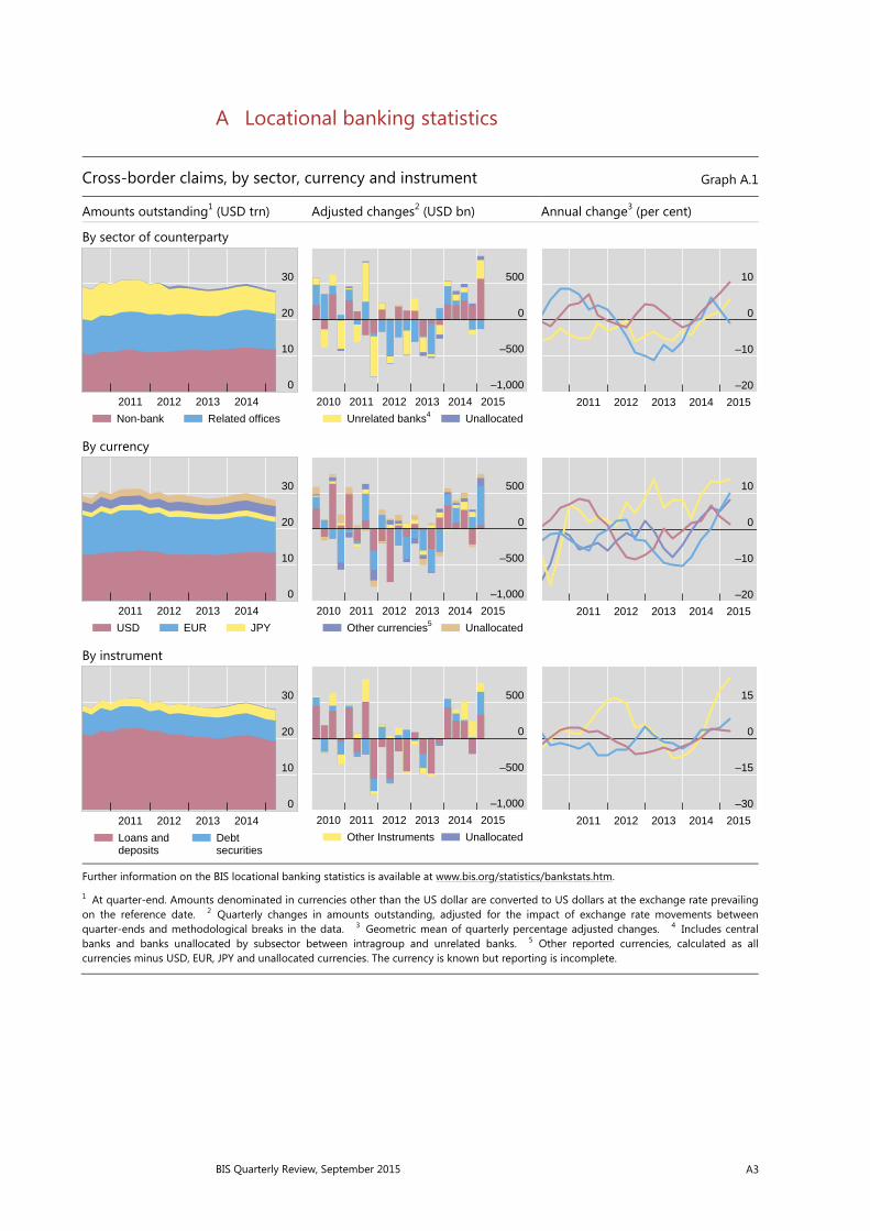
BIS Quarterly Review, September 2015 A3
A Locational banking statistics
Cross-border claims, by sector, currency and instrument Graph A.1
Amounts outstanding1 (USD trn) Adjusted changes2 (USD bn) Annual change3 (per cent)
By sector of counterparty
By currency
By instrument
Further information on the BIS locational banking statistics is available at www.bis.org/statistics/bankstats.htm.
1 At quarter-end. Amounts denominated in currencies other than the US dollar are converted to US dollars at the exchange rate prevailingon the reference date. 2 Quarterly changes in amounts outstanding, adjusted for the impact of exchange rate movements between quarter-ends and methodological breaks in the data. 3 Geometric mean of quarterly percentage adjusted changes. 4 Includes central banks and banks unallocated by subsector between intragroup and unrelated banks. 5 Other reported currencies, calculated as all currencies minus USD, EUR, JPY and unallocated currencies. The currency is known but reporting is incomplete.
0
10
20
30
2011 2012 2013 2014
Non-bank Related offices
–1,000
–500
0
500
2010 2011 2012 2013 2014 2015
Unrelated banks4 Unallocated
–20
–10
0
10
2011 2012 2013 2014 2015
0
10
20
30
2011 2012 2013 2014
USD EUR JPY
–1,000
–500
0
500
2010 2011 2012 2013 2014 2015
Other currencies5 Unallocated
–20
–10
0
10
2011 2012 2013 2014 2015
0
10
20
30
2011 2012 2013 2014
Loans and deposits
Debt securities
–1,000
–500
0
500
2010 2011 2012 2013 2014 2015
Other Instruments Unallocated
–30
–15
0
15
2011 2012 2013 2014 2015

A4 BIS Quarterly Review, September 2015
Cross-border claims, by borrowing region Graph A.2
Amounts outstanding1 (USD trn) Adjusted changes2 (USD bn) Annual change3 (per cent)
On all countries
On offshore centres
On emerging market economies
Further information on the BIS locational banking statistics is available at www.bis.org/statistics/bankstats.htm.
1 At quarter-end. Amounts denominated in currencies other than the US dollar are converted to US dollars at the exchange rate prevailingon the reference date. 2 Quarterly changes in amounts outstanding, adjusted for the impact of exchange rate movements betweenquarter-ends and methodological breaks in the data. 3 Geometric mean of quarterly percentage adjusted changes. 4 Includes international organisations and cross-border amounts unallocated by residence of counterparty.
0
10
20
30
2011 2012 2013 2014
Euro area Other European advanced
–1,000
–500
0
500
2010 2011 2012 2013 2014 2015
Other advanced4
Offshore centres
EMEs
–30
–15
0
15
2011 2012 2013 2014 2015
0
1
2
3
4
2011 2012 2013 2014
Caribbeanoffshore
Asian offshore
–300
–200
–100
0
100
2010 2011 2012 2013 2014 2015
Other offshore
–45
–30
–15
0
15
2011 2012 2013 2014 2015
0
1
2
3
2011 2012 2013 2014
Emerging Asia and Pacific
Emerging Europe
–200
0
200
400
2010 2011 2012 2013 2014 2015
Emerging LatinAmerica andCaribbean
Emerging Africaand Middle East
–20
0
20
40
2011 2012 2013 2014 2015

BIS Quarterly Review, September 2015 A5
Cross-border claims, by borrowing country Graph A.3
Amounts outstanding1 (USD trn) Adjusted changes2 (USD bn) Annual change3 (per cent)
On selected advanced economies
On selected offshore centres
On selected emerging market economies
Further information on the BIS locational banking statistics is available at www.bis.org/statistics/bankstats.htm.
1 At quarter-end. Amounts denominated in currencies other than the US dollar are converted to US dollars at the exchange rate prevailingon the reference date. 2 Quarterly changes in amounts outstanding, adjusted for the impact of exchange rate movements between quarter-ends and methodological breaks in the data. 3 Geometric mean of quarterly percentage adjusted changes.
0
5
10
15
2011 2012 2013 2014
United States United Kingdom
–600
–300
0
300
2010 2011 2012 2013 2014 2015
France Germany Japan
–30
–15
0
15
2011 2012 2013 2014 2015
0
1
2
3
2011 2012 2013 2014
Cayman Islands Hong Kong SAR
–300
–150
0
150
2010 2011 2012 2013 2014 2015
Singapore Jersey Bahamas
–60
–30
0
30
2011 2012 2013 2014 2015
0.0
0.5
1.0
1.5
2011 2012 2013 2014 2015
China Brazil India
–100
0
100
200
2010 2011 2012 2013 2014 2015
Russia South Africa
–50
0
50
100
2011 2012 2013 2014 2015
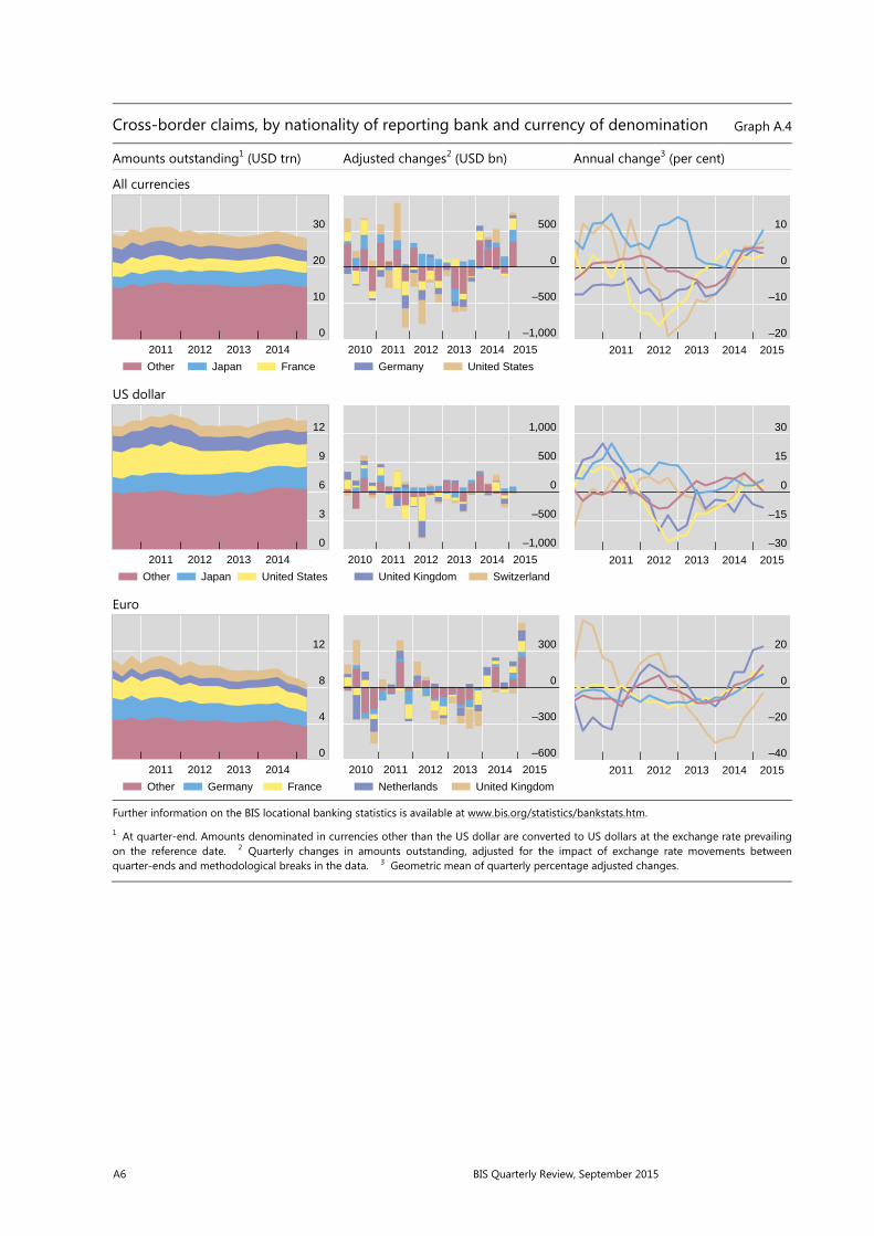
A6 BIS Quarterly Review, September 2015
Cross-border claims, by nationality of reporting bank and currency of denomination Graph A.4
Amounts outstanding1 (USD trn) Adjusted changes2 (USD bn) Annual change3 (per cent)
All currencies
US dollar
Euro
Further information on the BIS locational banking statistics is available at www.bis.org/statistics/bankstats.htm.
1 At quarter-end. Amounts denominated in currencies other than the US dollar are converted to US dollars at the exchange rate prevailingon the reference date. 2 Quarterly changes in amounts outstanding, adjusted for the impact of exchange rate movements betweenquarter-ends and methodological breaks in the data. 3 Geometric mean of quarterly percentage adjusted changes.
0
10
20
30
2011 2012 2013 2014
Other Japan France
–1,000
–500
0
500
2010 2011 2012 2013 2014 2015
Germany United States
–20
–10
0
10
2011 2012 2013 2014 2015
0
3
6
9
12
2011 2012 2013 2014
Other Japan United States
–1,000
–500
0
500
1,000
2010 2011 2012 2013 2014 2015
United Kingdom Switzerland
–30
–15
0
15
30
2011 2012 2013 2014 2015
0
4
8
12
2011 2012 2013 2014
Other Germany France
–600
–300
0
300
2010 2011 2012 2013 2014 2015
Netherlands United Kingdom
–40
–20
0
20
2011 2012 2013 2014 2015
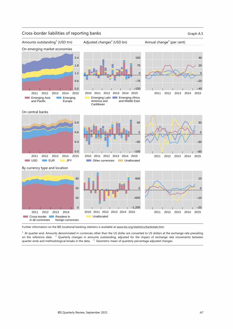
BIS Quarterly Review, September 2015 A7
Cross-border liabilities of reporting banks Graph A.5
Amounts outstanding1 (USD trn) Adjusted changes2 (USD bn) Annual change3 (per cent)
On emerging market economies
On central banks
By currency type and location
Further information on the BIS locational banking statistics is available at www.bis.org/statistics/bankstats.htm.
1 At quarter-end. Amounts denominated in currencies other than the US dollar are converted to US dollars at the exchange rate prevailing on the reference date. 2 Quarterly changes in amounts outstanding, adjusted for the impact of exchange rate movements betweenquarter-ends and methodological breaks in the data. 3 Geometric mean of quarterly percentage adjusted changes.
0.0
0.6
1.2
1.8
2.4
2011 2012 2013 2014 2015
Emerging Asia and Pacific
Emerging Europe
–150
–75
0
75
150
2010 2011 2012 2013 2014 2015
Emerging LatinAmerica andCaribbean
Emerging Africaand Middle East
–40
–20
0
20
40
2011 2012 2013 2014 2015
0.0
0.3
0.6
0.9
2011 2012 2013 2014 2015
USD EUR JPY
–100
–50
0
50
2010 2011 2012 2013 2014 2015
Other currencies Unallocated
–60
–30
0
30
2011 2012 2013 2014 2015
0
10
20
30
2011 2012 2013 2014
Cross-border in all currencies
Resident in foreign currencies
–1,200
–600
0
600
2010 2011 2012 2013 2014 2015
Unallocated
–20
–10
0
10
2011 2012 2013 2014 2015
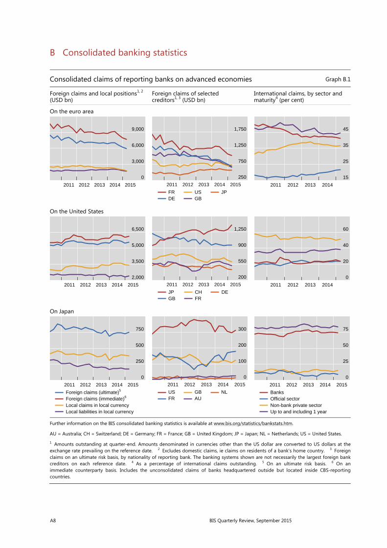
A8 BIS Quarterly Review, September 2015
B Consolidated banking statistics
Consolidated claims of reporting banks on advanced economies Graph B.1
Foreign claims and local positions1, 2 (USD bn)
Foreign claims of selected creditors1, 3 (USD bn)
International claims, by sector and maturity4 (per cent)
On the euro area
On the United States
On Japan
Further information on the BIS consolidated banking statistics is available at www.bis.org/statistics/bankstats.htm.
AU = Australia; CH = Switzerland; DE = Germany; FR = France; GB = United Kingdom; JP = Japan; NL = Netherlands; US = United States.
1 Amounts outstanding at quarter-end. Amounts denominated in currencies other than the US dollar are converted to US dollars at theexchange rate prevailing on the reference date. 2 Excludes domestic claims, ie claims on residents of a bank’s home country. 3 Foreign claims on an ultimate risk basis, by nationality of reporting bank. The banking systems shown are not necessarily the largest foreign bank creditors on each reference date. 4 As a percentage of international claims outstanding. 5 On an ultimate risk basis. 6 On an immediate counterparty basis. Includes the unconsolidated claims of banks headquartered outside but located inside CBS-reporting countries.
0
3,000
6,000
9,000
2011 2012 2013 2014 2015
250
750
1,250
1,750
2011 2012 2013 2014 2015
FRDE
USGB
JP
15
25
35
45
2011 2012 2013 2014
2,000
3,500
5,000
6,500
2011 2012 2013 2014 2015
200
550
900
1,250
2011 2012 2013 2014 2015
JPGB
CHFR
DE
0
20
40
60
2011 2012 2013 2014
0
250
500
750
2011 2012 2013 2014 2015
Foreign claims (ultimate)5
Foreign claims (immediate)6
Local claims in local currencyLocal liabilities in local currency
0
100
200
300
2011 2012 2013 2014 2015
USFR
GBAU
NL
0
25
50
75
2011 2012 2013 2014 2015
BanksOfficial sectorNon-bank private sectorUp to and including 1 year
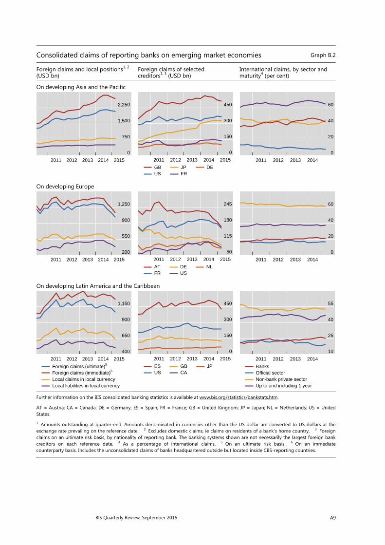
BIS Quarterly Review, September 2015 A9
Consolidated claims of reporting banks on emerging market economies Graph B.2
Foreign claims and local positions1, 2 (USD bn)
Foreign claims of selected creditors1, 3 (USD bn)
International claims, by sector and maturity4 (per cent)
On developing Asia and the Pacific
On developing Europe
On developing Latin America and the Caribbean
Further information on the BIS consolidated banking statistics is available at www.bis.org/statistics/bankstats.htm.
AT = Austria; CA = Canada; DE = Germany; ES = Spain; FR = France; GB = United Kingdom; JP = Japan; NL = Netherlands; US = United States.
1 Amounts outstanding at quarter-end. Amounts denominated in currencies other than the US dollar are converted to US dollars at the exchange rate prevailing on the reference date. 2 Excludes domestic claims, ie claims on residents of a bank’s home country. 3 Foreign claims on an ultimate risk basis, by nationality of reporting bank. The banking systems shown are not necessarily the largest foreign bank creditors on each reference date. 4 As a percentage of international claims. 5 On an ultimate risk basis. 6 On an immediate counterparty basis. Includes the unconsolidated claims of banks headquartered outside but located inside CBS-reporting countries.
0
750
1,500
2,250
2011 2012 2013 2014 2015
0
150
300
450
2011 2012 2013 2014 2015
GBUS
JPFR
DE
0
20
40
60
2011 2012 2013 2014
200
550
900
1,250
2011 2012 2013 2014 2015
50
115
180
245
2011 2012 2013 2014 2015
ATFR
DEUS
NL
0
20
40
60
2011 2012 2013 2014
400
650
900
1,150
2011 2012 2013 2014 2015
Foreign claims (ultimate)5
Foreign claims (immediate)6
Local claims in local currencyLocal liabilities in local currency
0
150
300
450
2011 2012 2013 2014 2015
ESUS
GBCA
JP
10
25
40
55
2011 2012 2013 2014
BanksOfficial sectorNon-bank private sectorUp to and including 1 year
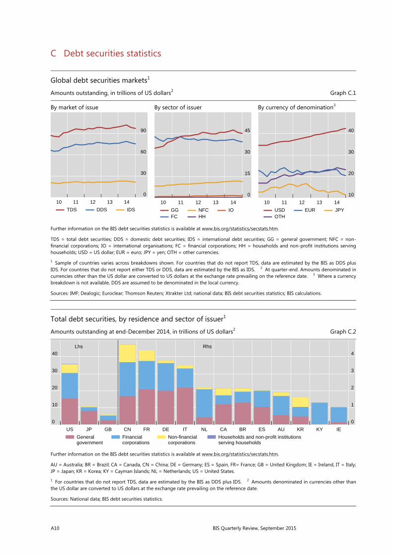
A10 BIS Quarterly Review, September 2015
C Debt securities statistics
Global debt securities markets1
Amounts outstanding, in trillions of US dollars2 Graph C.1
By market of issue By sector of issuer By currency of denomination3
Further information on the BIS debt securities statistics is available at www.bis.org/statistics/secstats.htm.
TDS = total debt securities; DDS = domestic debt securities; IDS = international debt securities; GG = general government; NFC = non-financial corporations; IO = international organisations; FC = financial corporations; HH = households and non-profit institutions serving households; USD = US dollar; EUR = euro; JPY = yen; OTH = other currencies.
1 Sample of countries varies across breakdowns shown. For countries that do not report TDS, data are estimated by the BIS as DDS plus IDS. For countries that do not report either TDS or DDS, data are estimated by the BIS as IDS. 2 At quarter-end. Amounts denominated in currencies other than the US dollar are converted to US dollars at the exchange rate prevailing on the reference date. 3 Where a currency breakdown is not available, DDS are assumed to be denominated in the local currency.
Sources: IMF; Dealogic; Euroclear; Thomson Reuters; Xtrakter Ltd; national data; BIS debt securities statistics; BIS calculations.
Total debt securities, by residence and sector of issuer1
Amounts outstanding at end-December 2014, in trillions of US dollars2 Graph C.2
Further information on the BIS debt securities statistics is available at www.bis.org/statistics/secstats.htm.
AU = Australia; BR = Brazil; CA = Canada, CN = China; DE = Germany; ES = Spain, FR= France; GB = United Kingdom; IE = Ireland, IT = Italy;JP = Japan; KR = Korea; KY = Cayman Islands; NL = Netherlands; US = United States.
1 For countries that do not report TDS, data are estimated by the BIS as DDS plus IDS. 2 Amounts denominated in currencies other than the US dollar are converted to US dollars at the exchange rate prevailing on the reference date.
Sources: National data; BIS debt securities statistics.
0
30
60
90
10 11 12 13 14
TDS DDS IDS
0
15
30
45
10 11 12 13 14
GGFC
NFCHH
IO
10
20
30
40
10 11 12 13 14
USDOTH
EUR JPY
0
10
20
30
40
0
1
2
3
4
US JP GB CN FR DE IT NL CA BR ES AU KR KY IE
Lhs Rhs
General government
Financial corporations
Non-financial corporations
Households and non-profit institutions serving households
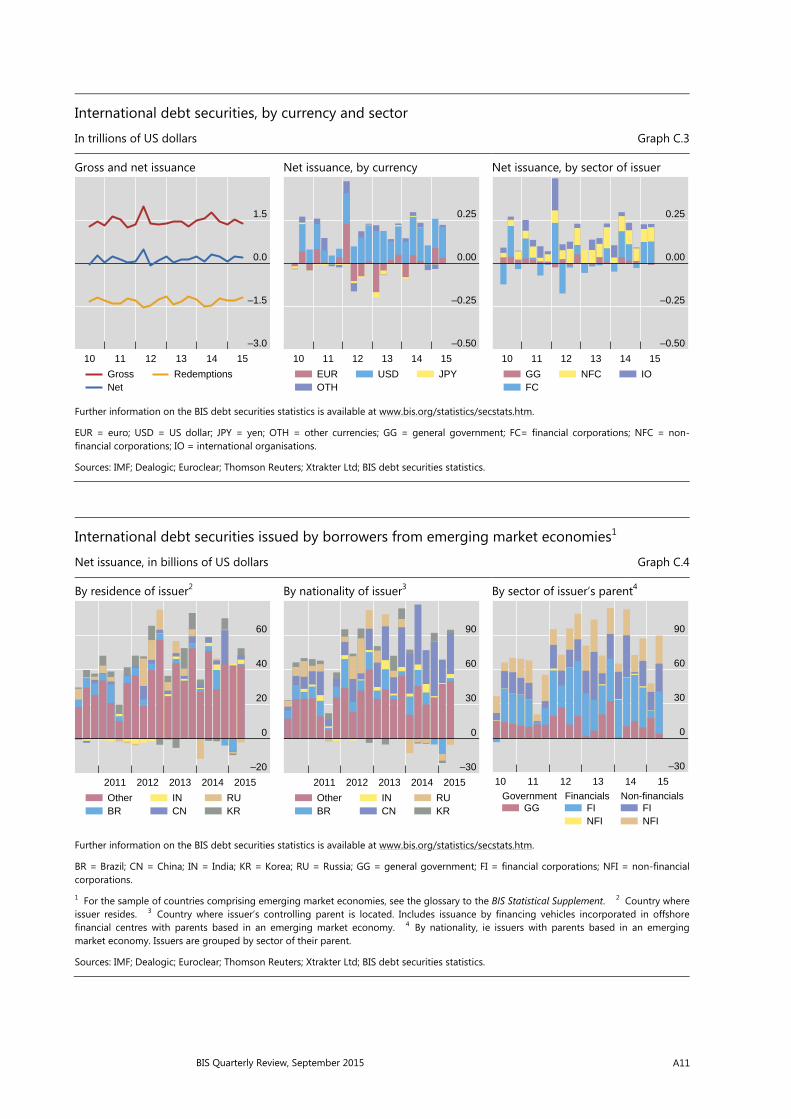
BIS Quarterly Review, September 2015 A11
International debt securities, by currency and sector
In trillions of US dollars Graph C.3
Gross and net issuance Net issuance, by currency Net issuance, by sector of issuer
Further information on the BIS debt securities statistics is available at www.bis.org/statistics/secstats.htm.
EUR = euro; USD = US dollar; JPY = yen; OTH = other currencies; GG = general government; FC= financial corporations; NFC = non-financial corporations; IO = international organisations.
Sources: IMF; Dealogic; Euroclear; Thomson Reuters; Xtrakter Ltd; BIS debt securities statistics.
International debt securities issued by borrowers from emerging market economies1
Net issuance, in billions of US dollars Graph C.4
By residence of issuer2 By nationality of issuer3 By sector of issuer’s parent4
Further information on the BIS debt securities statistics is available at www.bis.org/statistics/secstats.htm.
BR = Brazil; CN = China; IN = India; KR = Korea; RU = Russia; GG = general government; FI = financial corporations; NFI = non-financial corporations.
1 For the sample of countries comprising emerging market economies, see the glossary to the BIS Statistical Supplement. 2 Country where issuer resides. 3 Country where issuer’s controlling parent is located. Includes issuance by financing vehicles incorporated in offshorefinancial centres with parents based in an emerging market economy. 4 By nationality, ie issuers with parents based in an emerging market economy. Issuers are grouped by sector of their parent.
Sources: IMF; Dealogic; Euroclear; Thomson Reuters; Xtrakter Ltd; BIS debt securities statistics.
–3.0
–1.5
0.0
1.5
10 11 12 13 14 15
GrossNet
Redemptions
–0.50
–0.25
0.00
0.25
10 11 12 13 14 15
EUROTH
USD JPY
–0.50
–0.25
0.00
0.25
10 11 12 13 14 15
GGFC
NFC IO
–20
0
20
40
60
2011 2012 2013 2014 2015
OtherBR
INCN
RUKR
–30
0
30
60
90
2011 2012 2013 2014 2015
OtherBR
INCN
RUKR
–30
0
30
60
90
10 11 12 13 14 15
GGGovernment
FINFI
FinancialsFINFI
Non-financials
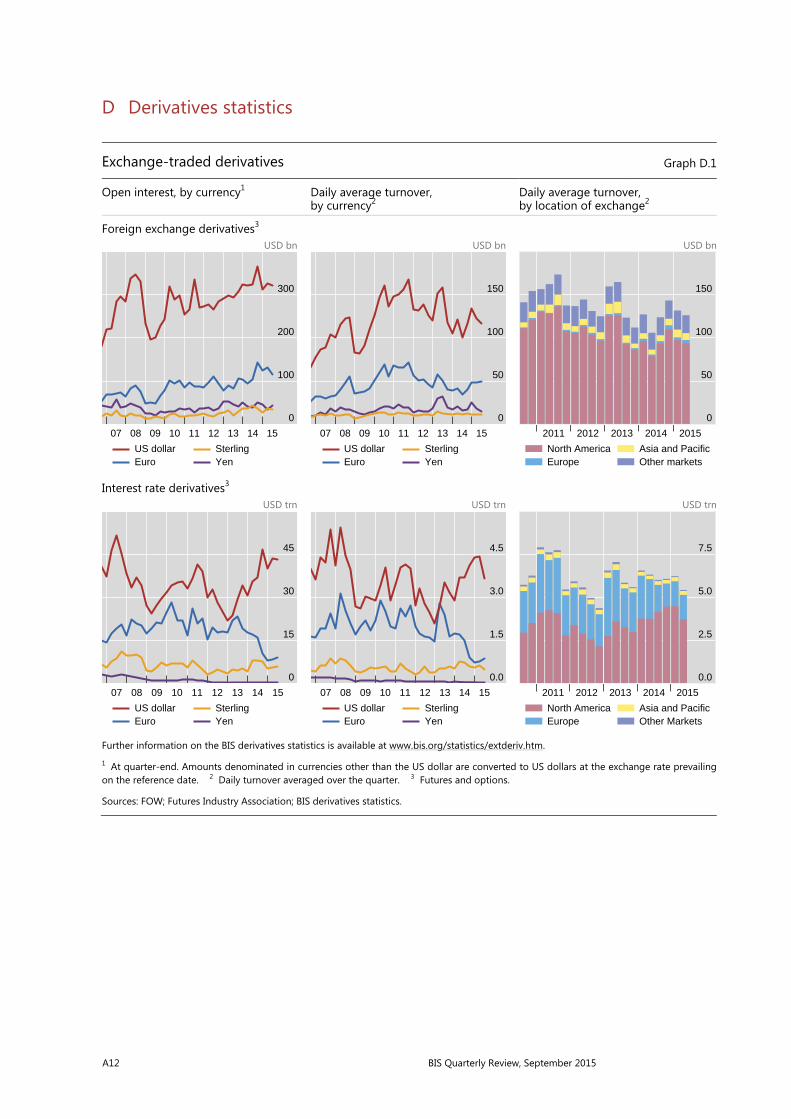
A12 BIS Quarterly Review, September 2015
D Derivatives statistics
Exchange-traded derivatives Graph D.1
Open interest, by currency1 Daily average turnover, by currency2
Daily average turnover, by location of exchange2
Foreign exchange derivatives3 USD bn USD bn USD bn
Interest rate derivatives3 USD trn USD trn USD trn
Further information on the BIS derivatives statistics is available at www.bis.org/statistics/extderiv.htm.
1 At quarter-end. Amounts denominated in currencies other than the US dollar are converted to US dollars at the exchange rate prevailing on the reference date. 2 Daily turnover averaged over the quarter. 3 Futures and options.
Sources: FOW; Futures Industry Association; BIS derivatives statistics.
0
100
200
300
07 08 09 10 11 12 13 14 15
US dollarEuro
SterlingYen
0
50
100
150
07 08 09 10 11 12 13 14 15
US dollarEuro
SterlingYen
0
50
100
150
2011 2012 2013 2014 2015
North AmericaEurope
Asia and PacificOther markets
0
15
30
45
07 08 09 10 11 12 13 14 15
US dollarEuro
SterlingYen
0.0
1.5
3.0
4.5
07 08 09 10 11 12 13 14 15
US dollarEuro
SterlingYen
0.0
2.5
5.0
7.5
2011 2012 2013 2014 2015
North AmericaEurope
Asia and PacificOther Markets
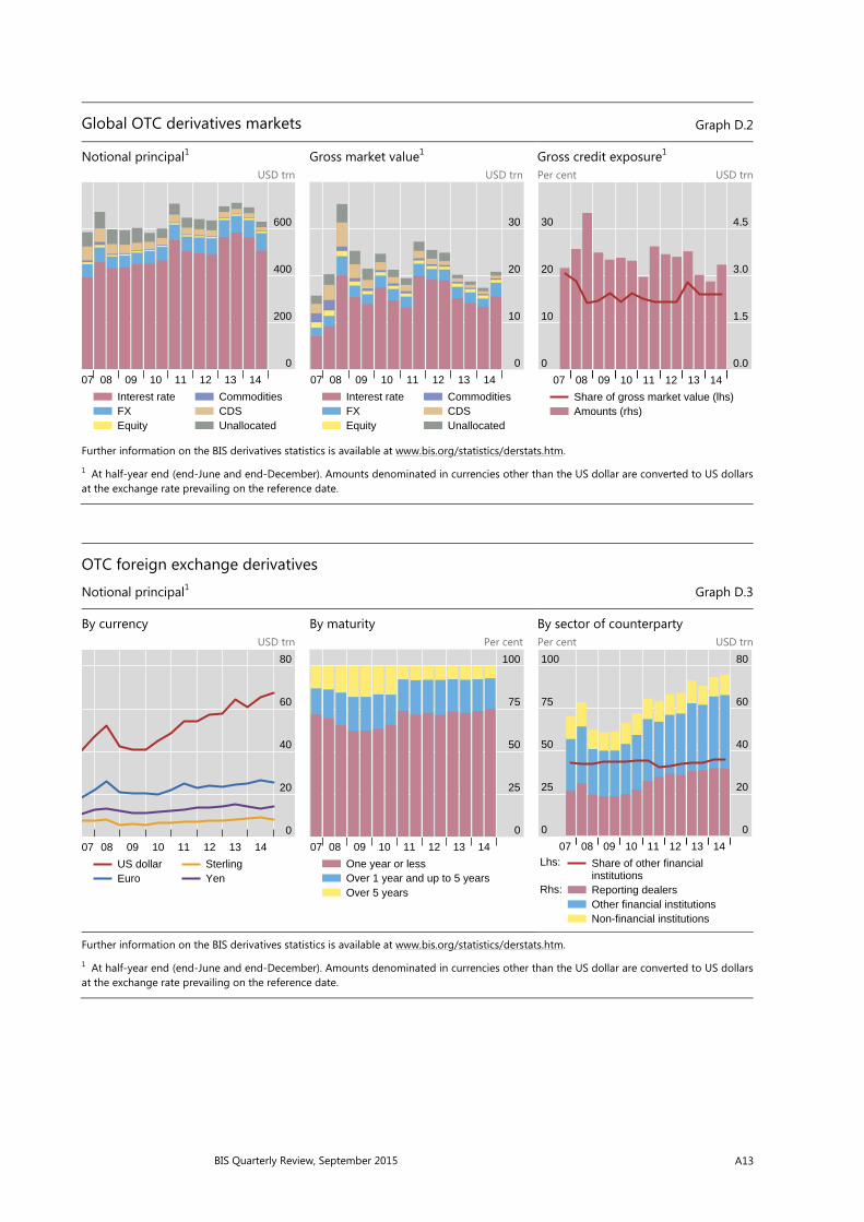
BIS Quarterly Review, September 2015 A13
Global OTC derivatives markets Graph D.2
Notional principal1 Gross market value1 Gross credit exposure1 USD trn USD trn Per cent USD trn
Further information on the BIS derivatives statistics is available at www.bis.org/statistics/derstats.htm.
1 At half-year end (end-June and end-December). Amounts denominated in currencies other than the US dollar are converted to US dollarsat the exchange rate prevailing on the reference date.
OTC foreign exchange derivatives
Notional principal1 Graph D.3
By currency By maturity By sector of counterparty USD trn Per cent Per cent USD trn
Further information on the BIS derivatives statistics is available at www.bis.org/statistics/derstats.htm.
1 At half-year end (end-June and end-December). Amounts denominated in currencies other than the US dollar are converted to US dollars at the exchange rate prevailing on the reference date.
0
200
400
600
07 08 09 10 11 12 13 14
Interest rateFXEquity
CommoditiesCDSUnallocated
0
10
20
30
07 08 09 10 11 12 13 14
Interest rateFXEquity
CommoditiesCDSUnallocated
0
10
20
30
0.0
1.5
3.0
4.5
07 08 09 10 11 12 13 14
Share of gross market value (lhs)Amounts (rhs)
0
20
40
60
80
07 08 09 10 11 12 13 14
US dollarEuro
SterlingYen
0
25
50
75
100
07 08 09 10 11 12 13 14
One year or lessOver 1 year and up to 5 yearsOver 5 years
0
25
50
75
100
0
20
40
60
80
07 08 09 10 11 12 13 14Lhs:
Rhs:
Share of other financial institutionsReporting dealersOther financial institutionsNon-financial institutions
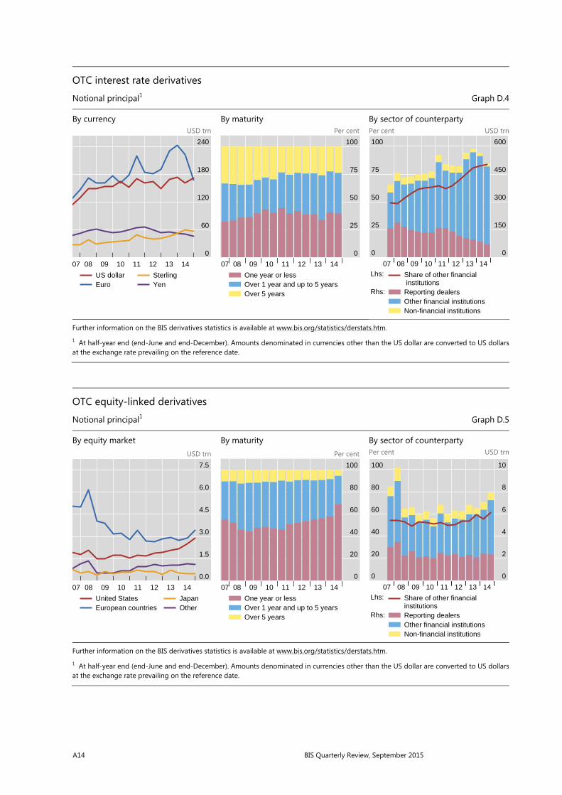
A14 BIS Quarterly Review, September 2015
OTC interest rate derivatives
Notional principal1 Graph D.4
By currency By maturity By sector of counterparty USD trn Per cent Per cent USD trn
Further information on the BIS derivatives statistics is available at www.bis.org/statistics/derstats.htm.
1 At half-year end (end-June and end-December). Amounts denominated in currencies other than the US dollar are converted to US dollars at the exchange rate prevailing on the reference date.
OTC equity-linked derivatives
Notional principal1 Graph D.5
By equity market By maturity By sector of counterparty USD trn Per cent Per cent USD trn
Further information on the BIS derivatives statistics is available at www.bis.org/statistics/derstats.htm.
1 At half-year end (end-June and end-December). Amounts denominated in currencies other than the US dollar are converted to US dollars at the exchange rate prevailing on the reference date.
0
60
120
180
240
07 08 09 10 11 12 13 14
US dollarEuro
SterlingYen
0
25
50
75
100
07 08 09 10 11 12 13 14
One year or lessOver 1 year and up to 5 yearsOver 5 years
0
25
50
75
100
0
150
300
450
600
07 08 09 10 11 12 13 14Lhs:
Rhs:
Share of other financial institutionsReporting dealersOther financial institutionsNon-financial institutions
0.0
1.5
3.0
4.5
6.0
7.5
07 08 09 10 11 12 13 14
United StatesEuropean countries
JapanOther
0
20
40
60
80
100
07 08 09 10 11 12 13 14
One year or lessOver 1 year and up to 5 yearsOver 5 years
0
20
40
60
80
100
0
2
4
6
8
10
07 08 09 10 11 12 13 14Lhs:
Rhs:
Share of other financial institutionsReporting dealersOther financial institutionsNon-financial institutions
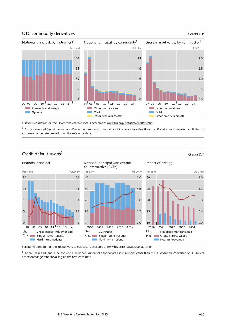
BIS Quarterly Review, September 2015 A15
OTC commodity derivatives Graph D.6
Notional principal, by instrument1 Notional principal, by commodity1 Gross market value, by commodity1 Per cent USD bn USD trn
Further information on the BIS derivatives statistics is available at www.bis.org/statistics/derstats.htm.
1 At half-year end (end-June and end-December). Amounts denominated in currencies other than the US dollar are converted to US dollars at the exchange rate prevailing on the reference date.
Credit default swaps1 Graph D.7
Notional principal Notional principal with central counterparties (CCPs)
Impact of netting
Per cent USD trn Per cent USD trn Per cent USD trn
Further information on the BIS derivatives statistics is available at www.bis.org/statistics/derstats.htm.
1 At half-year end (end-June and end-December). Amounts denominated in currencies other than the US dollar are converted to US dollarsat the exchange rate prevailing on the reference date.
0
25
50
75
100
07 08 09 10 11 12 13 14
Forwards and swapsOptions
0
3
6
9
12
07 08 09 10 11 12 13 14
Other commoditiesGoldOther precious metals
0.0
0.5
1.0
1.5
2.0
07 08 09 10 11 12 13 14
Other commoditiesGoldOther precious metals
0
5
10
15
20
0
15
30
45
60
07 08 09 10 11 12 13 14
Lhs:Rhs:
Gross market value/notionalSingle-name notionalMulti-name notional
0
10
20
30
40
0.0
1.5
3.0
4.5
6.0
2010 2011 2012 2013 2014Lhs:Rhs:
CCPs/totalSingle-name notionalMulti-name notional
10
15
20
25
30
0.0
0.4
0.8
1.2
1.6
2010 2011 2012 2013 2014Lhs:Rhs:
Net/gross market valuesGross market valuesNet market values

A16 BIS Quarterly Review, September 2015
Concentration in global OTC derivatives markets
Herfindahl index1 Graph D.8
Foreign exchange derivatives2 Interest rate swaps Equity-linked options
Further information on the BIS derivatives statistics is available at www.bis.org/statistics/derstats.htm.
CAD = Canadian dollar; CHF = Swiss franc; EUR = euro; GBP = pound sterling; JPY = Japanese yen; SEK = Swedish krona; USD = US dollar.JP = Japan; US = United States.
1 The index ranges from 0 to 10,000, where a lower number indicates that there are many dealers with similar market shares (as measuredby notional principal) and a higher number indicates that the market is dominated by a few reporting dealers. 2 Foreign exchange forwards, foreign exchange swaps and currency swaps.
400
600
800
1,000
07 08 09 10 11 12 13 14
USDEURGBP
JPYCHFCAD
SEK
400
850
1,300
1,750
07 08 09 10 11 12 13 14
USDEURGBP
JPYCHFCAD
SEK
400
2,300
4,200
6,100
07 08 09 10 11 12 13 14
USJP
EuropeLatin America
Other Asian

BIS Quarterly Review, September 2015 A17
E Global liquidity indicators
Growth of international bank credit1 Graph E.1
Volatility, in per cent Annual change, in per cent
Further information on the BIS global liquidity indicators is available at www.bis.org/statistics/gli.htm.
1 LBS reporting banks’ cross-border claims plus local claims in foreign currencies. 2 VIX refers to the Chicago Board Options Exchange Market Volatility Index. It measures the implied volatility of S&P 500 index options. 3 Contribution to the annual percentage change incredit to all sectors. 4 Including intragroup transactions.
Sources: Bloomberg; BIS locational banking statistics.
0
16
32
48
–10
0
10
20
78 80 82 84 86 88 90 92 94 96 98 00 02 04 06 08 10 12 14
Rhs:Lhs: VIX2 Credit to non-banks3 Credit to banks3,4

A18 BIS Quarterly Review, September 2015
Global bank credit to the non-bank sector, by residence of borrower
Banks’ cross-border credit plus local credit in all currencies1 Graph E.2
All countries2 United States Euro area USD trn Per cent USD trn Per cent USD trn Per cent
Emerging Asia USD trn Per cent
Latin America USD trn Per cent
Emerging Europe USD trn Per cent
Further information on the BIS global liquidity indicators is available at www.bis.org/statistics/gli.htm.
1 Cross-border claims of LBS reporting banks plus local claims of all banks. Local claims are from national financial accounts and include credit extended by the central bank to the government. 2 Sample of 52 countries. 3 Amounts outstanding at quarter-end. Amounts denominated in currencies other than the US dollar are converted to US dollars at the exchange rate prevailing at end-March 2015.
Sources: IMF, International Financial Statistics; BIS locational banking statistics; BIS calculations.
0
25
50
75
100
–24
–12
0
12
24
01 03 05 07 09 11 13 15
0
5
10
15
20
–24
–12
0
12
24
01 03 05 07 09 11 13 15
0
5
10
15
20
–24
–12
0
12
24
01 03 05 07 09 11 13 15
0
6
12
18
24
–50
–25
0
25
50
01 03 05 07 09 11 13 15
Cross-border creditLocal credit
Amounts outstanding3 (lhs):
0.0
0.8
1.6
2.4
3.2
–40
–20
0
20
40
01 03 05 07 09 11 13 15
Cross-border creditLocal credit
Annual change (rhs):
0.0
0.3
0.6
0.9
1.2
–40
–20
0
20
40
01 03 05 07 09 11 13 15
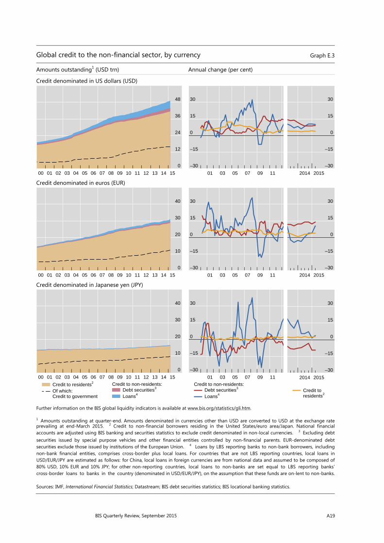
BIS Quarterly Review, September 2015 A19
Global credit to the non-financial sector, by currency Graph E.3
Amounts outstanding1 (USD trn) Annual change (per cent)
Credit denominated in US dollars (USD)
Credit denominated in euros (EUR)
Credit denominated in Japanese yen (JPY)
Further information on the BIS global liquidity indicators is available at www.bis.org/statistics/gli.htm.
1 Amounts outstanding at quarter-end. Amounts denominated in currencies other than USD are converted to USD at the exchange rate prevailing at end-March 2015. 2 Credit to non-financial borrowers residing in the United States/euro area/Japan. National financial accounts are adjusted using BIS banking and securities statistics to exclude credit denominated in non-local currencies. 3 Excluding debt securities issued by special purpose vehicles and other financial entities controlled by non-financial parents. EUR-denominated debt securities exclude those issued by institutions of the European Union. 4 Loans by LBS reporting banks to non-bank borrowers, including non-bank financial entities, comprises cross-border plus local loans. For countries that are not LBS reporting countries, local loans in USD/EUR/JPY are estimated as follows: for China, local loans in foreign currencies are from national data and assumed to be composed of 80% USD, 10% EUR and 10% JPY; for other non-reporting countries, local loans to non-banks are set equal to LBS reporting banks’ cross-border loans to banks in the country (denominated in USD/EUR/JPY), on the assumption that these funds are on-lent to non-banks.
Sources: IMF, International Financial Statistics; Datastream; BIS debt securities statistics; BIS locational banking statistics.
0
12
24
36
48
00 01 02 03 04 05 06 07 08 09 10 11 12 13 14 15
–30
–15
0
15
30
01 03 05 07 09 11
–30
–15
0
15
30
2014 2015
0
10
20
30
40
00 01 02 03 04 05 06 07 08 09 10 11 12 13 14 15
–30
–15
0
15
30
01 03 05 07 09 11
–30
–15
0
15
30
2014 2015
0
10
20
30
40
00 01 02 03 04 05 06 07 08 09 10 11 12 13 14 15
Credit to residents2
Of which: Credit to government
Debt securities3
Loans4
Credit to non-residents:
–30
–15
0
15
30
01 03 05 07 09 11
Debt securities3
Loans4
Credit to non-residents:
–30
–15
0
15
30
2014 2015
Credit toresidents2
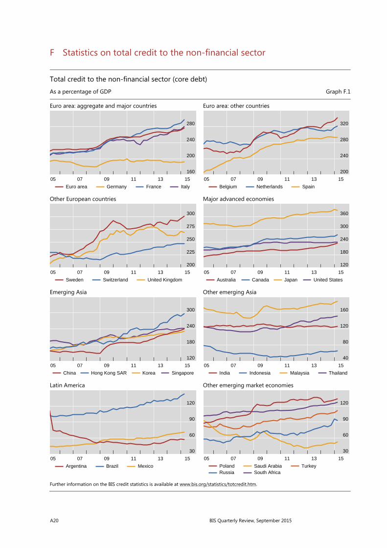
A20 BIS Quarterly Review, September 2015
F Statistics on total credit to the non-financial sector
Total credit to the non-financial sector (core debt)
As a percentage of GDP Graph F.1
Euro area: aggregate and major countries Euro area: other countries
Other European countries Major advanced economies
Emerging Asia Other emerging Asia
Latin America Other emerging market economies
Further information on the BIS credit statistics is available at www.bis.org/statistics/totcredit.htm.
160
200
240
280
05 07 09 11 13 15
Euro area Germany France Italy
200
240
280
320
05 07 09 11 13 15
Belgium Netherlands Spain
200
225
250
275
300
05 07 09 11 13 15
Sweden Switzerland United Kingdom
120
180
240
300
360
05 07 09 11 13 15
Australia Canada Japan United States
120
180
240
300
05 07 09 11 13 15
China Hong Kong SAR Korea Singapore
40
80
120
160
05 07 09 11 13 15
India Indonesia Malaysia Thailand
30
60
90
120
05 07 09 11 13 15
Argentina Brazil Mexico
30
60
90
120
05 07 09 11 13 15
PolandRussia
Saudi ArabiaSouth Africa
Turkey
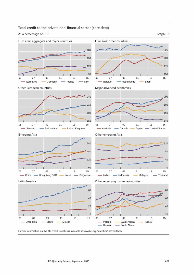
BIS Quarterly Review, September 2015 A21
Total credit to the private non-financial sector (core debt)
As a percentage of GDP Graph F.2
Euro area: aggregate and major countries Euro area: other countries
Other European countries Major advanced economies
Emerging Asia Other emerging Asia
Latin America Other emerging market economies
Further information on the BIS credit statistics is available at www.bis.org/statistics/totcredit.htm.
90
120
150
180
05 07 09 11 13 15
Euro area Germany France Italy
150
175
200
225
05 07 09 11 13 15
Belgium Netherlands Spain
150
180
210
240
05 07 09 11 13 15
Sweden Switzerland United Kingdom
140
160
180
200
05 07 09 11 13 15
Australia Canada Japan United States
60
120
180
240
05 07 09 11 13 15
China Hong Kong SAR Korea Singapore
0
40
80
120
05 07 09 11 13 15
India Indonesia Malaysia Thailand
0
20
40
60
05 07 09 11 13 15
Argentina Brazil Mexico
20
40
60
80
05 07 09 11 13 15
PolandRussia
Saudi ArabiaSouth Africa
Turkey

A22 BIS Quarterly Review, September 2015
Bank credit to the private non-financial sector (core debt)
As a percentage of GDP Graph F.3
Euro area: aggregate and major countries Euro area: other countries
Other European countries Major advanced economies
Emerging Asia Other emerging Asia
Latin America Other emerging market economies
Further information on the BIS credit statistics is available at www.bis.org/statistics/totcredit.htm.
60
70
80
90
100
05 07 09 11 13 15
Euro area Germany France Italy
50
75
100
125
150
05 07 09 11 13 15
Belgium Netherlands Spain
80
100
120
140
160
05 07 09 11 13 15
Sweden Switzerland United Kingdom
40
60
80
100
120
05 07 09 11 13 15
Australia Canada Japan United States
40
80
120
160
200
05 07 09 11 13 15
China Hong Kong SAR Korea Singapore
0
30
60
90
120
05 07 09 11 13 15
India Indonesia Malaysia Thailand
0
15
30
45
60
05 07 09 11 13 15
Argentina Brazil Mexico
15
30
45
60
75
05 07 09 11 13 15
PolandRussia
Saudi ArabiaSouth Africa
Turkey
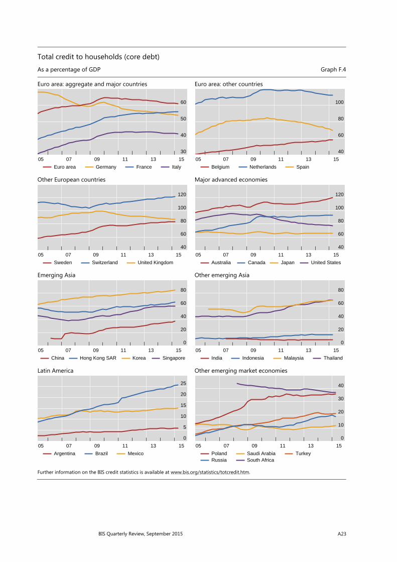
BIS Quarterly Review, September 2015 A23
Total credit to households (core debt)
As a percentage of GDP Graph F.4
Euro area: aggregate and major countries Euro area: other countries
Other European countries Major advanced economies
Emerging Asia Other emerging Asia
Latin America Other emerging market economies
Further information on the BIS credit statistics is available at www.bis.org/statistics/totcredit.htm.
30
40
50
60
05 07 09 11 13 15
Euro area Germany France Italy
40
60
80
100
05 07 09 11 13 15
Belgium Netherlands Spain
40
60
80
100
120
05 07 09 11 13 15
Sweden Switzerland United Kingdom
40
60
80
100
120
05 07 09 11 13 15
Australia Canada Japan United States
0
20
40
60
80
05 07 09 11 13 15
China Hong Kong SAR Korea Singapore
0
20
40
60
80
05 07 09 11 13 15
India Indonesia Malaysia Thailand
0
5
10
15
20
25
05 07 09 11 13 15
Argentina Brazil Mexico
0
10
20
30
40
05 07 09 11 13 15
PolandRussia
Saudi ArabiaSouth Africa
Turkey

A24 BIS Quarterly Review, September 2015
Total credit to non-financial corporations (core debt)
As a percentage of GDP Graph F.5
Euro area: aggregate and major countries Euro area: other countries
Other European countries Major advanced economies
Emerging Asia Other emerging Asia
Latin America Other emerging market economies
Further information on the BIS credit statistics is available at www.bis.org/statistics/totcredit.htm.
40
60
80
100
120
05 07 09 11 13 15
Euro area Germany France Italy
90
105
120
135
150
05 07 09 11 13 15
Belgium Netherlands Spain
50
75
100
125
150
05 07 09 11 13 15
Sweden Switzerland United Kingdom
60
70
80
90
100
05 07 09 11 13 15
Australia Canada Japan United States
50
100
150
200
05 07 09 11 13 15
China Hong Kong SAR Korea Singapore
10
25
40
55
05 07 09 11 13 15
India Indonesia Malaysia Thailand
0
15
30
45
05 07 09 11 13 15
Argentina Brazil Mexico
0
15
30
45
05 07 09 11 13 15
PolandRussia
Saudi ArabiaSouth Africa
Turkey
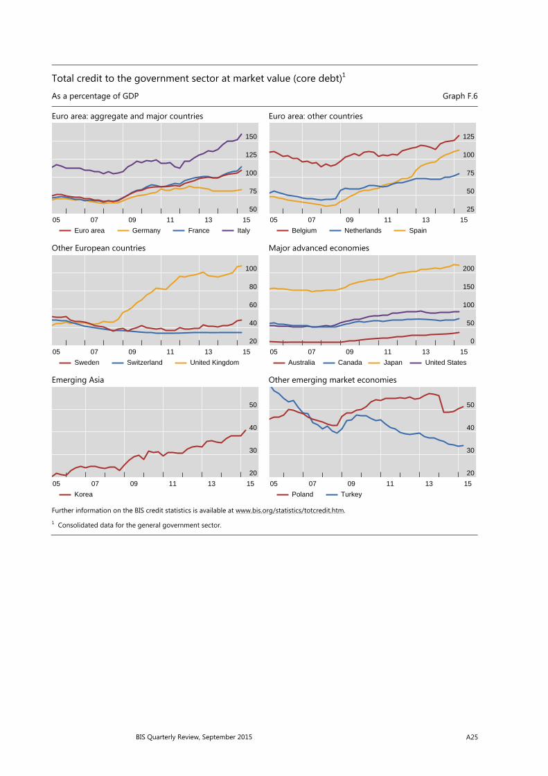
BIS Quarterly Review, September 2015 A25
Total credit to the government sector at market value (core debt)1
As a percentage of GDP Graph F.6
Euro area: aggregate and major countries Euro area: other countries
Other European countries Major advanced economies
Emerging Asia Other emerging market economies
Further information on the BIS credit statistics is available at www.bis.org/statistics/totcredit.htm.
1 Consolidated data for the general government sector.
50
75
100
125
150
05 07 09 11 13 15
Euro area Germany France Italy
25
50
75
100
125
05 07 09 11 13 15
Belgium Netherlands Spain
20
40
60
80
100
05 07 09 11 13 15
Sweden Switzerland United Kingdom
0
50
100
150
200
05 07 09 11 13 15
Australia Canada Japan United States
20
30
40
50
05 07 09 11 13 15
Korea
20
30
40
50
05 07 09 11 13 15
Poland Turkey
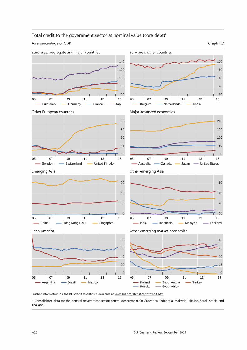
A26 BIS Quarterly Review, September 2015
Total credit to the government sector at nominal value (core debt)1
As a percentage of GDP Graph F.7
Euro area: aggregate and major countries Euro area: other countries
Other European countries Major advanced economies
Emerging Asia Other emerging Asia
Latin America Other emerging market economies
Further information on the BIS credit statistics is available at www.bis.org/statistics/totcredit.htm.
1 Consolidated data for the general government sector; central government for Argentina, Indonesia, Malaysia, Mexico, Saudi Arabia and Thailand.
60
80
100
120
140
05 07 09 11 13 15
Euro area Germany France Italy
20
40
60
80
100
05 07 09 11 13 15
Belgium Netherlands Spain
30
45
60
75
90
05 07 09 11 13 15
Sweden Switzerland United Kingdom
0
50
100
150
200
05 07 09 11 13 15
Australia Canada Japan United States
0
30
60
90
05 07 09 11 13 15
China Hong Kong SAR Singapore
20
40
60
80
05 07 09 11 13 15
India Indonesia Malaysia Thailand
0
20
40
60
80
05 07 09 11 13 15
Argentina Brazil Mexico
0
15
30
45
60
05 07 09 11 13 15
PolandRussia
Saudi ArabiaSouth Africa
Turkey
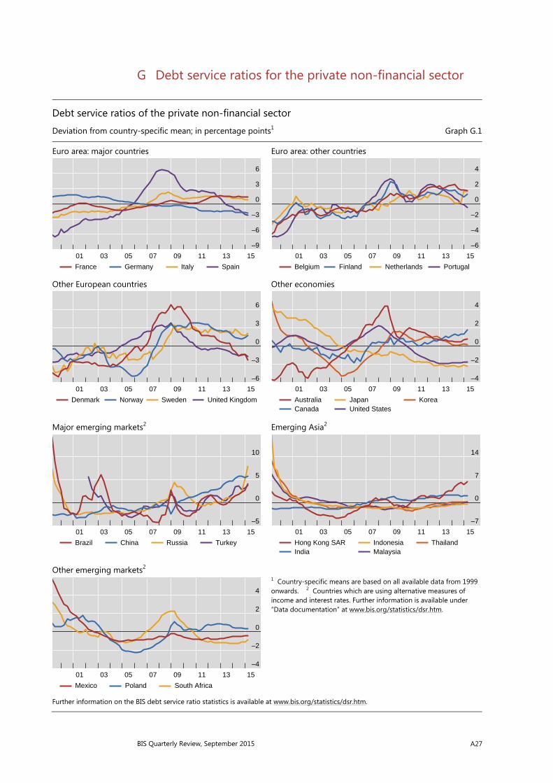
BIS Quarterly Review, September 2015 A27
G Debt service ratios for the private non-financial sector
Debt service ratios of the private non-financial sector
Deviation from country-specific mean; in percentage points1 Graph G.1
Euro area: major countries Euro area: other countries
Other European countries Other economies
Major emerging markets2 Emerging Asia2
Other emerging markets2
1 Country-specific means are based on all available data from 1999 onwards. 2 Countries which are using alternative measures of income and interest rates. Further information is available under “Data documentation” at www.bis.org/statistics/dsr.htm.
Further information on the BIS debt service ratio statistics is available at www.bis.org/statistics/dsr.htm.
–9
–6
–3
0
3
6
01 03 05 07 09 11 13 15
France Germany Italy Spain
–6
–4
–2
0
2
4
01 03 05 07 09 11 13 15
Belgium Finland Netherlands Portugal
–6
–3
0
3
6
01 03 05 07 09 11 13 15
Denmark Norway Sweden United Kingdom
–4
–2
0
2
4
01 03 05 07 09 11 13 15
AustraliaCanada
JapanUnited States
Korea
–5
0
5
10
01 03 05 07 09 11 13 15
Brazil China Russia Turkey
–7
0
7
14
01 03 05 07 09 11 13 15
Hong Kong SARIndia
IndonesiaMalaysia
Thailand
–4
–2
0
2
4
01 03 05 07 09 11 13 15
Mexico Poland South Africa

A28 BIS Quarterly Review, September 2015
Debt service ratios of households
Deviation from country-specific mean; in percentage points1 Graph G.2
Euro area: major countries Euro area: other countries
Other European countries Other economies
Further information on the BIS debt service ratio statistics is available at www.bis.org/statistics/dsr.htm.
1 Country-specific means are based on all available data from 1999 onwards.
–4
–2
0
2
4
01 03 05 07 09 11 13 15
France Germany Italy Spain
–6
–4
–2
0
2
01 03 05 07 09 11 13 15
Belgium Finland Netherlands Portugal
–4
–2
0
2
4
01 03 05 07 09 11 13 15
Denmark Norway Sweden United Kingdom
–6
–4
–2
0
2
01 03 05 07 09 11 13 15
AustraliaCanada
JapanUnited States
Korea

BIS Quarterly Review, September 2015 A29
Debt service ratios of non-financial corporations
Deviation from country-specific mean; in percentage points1 Graph G.3
Euro area: major countries Euro area: other countries
Other European countries Other economies
Further information on the BIS debt service ratio statistics is available at www.bis.org/statistics/dsr.htm.
1 Country-specific means are based on all available data from 1999 onwards.
–20
–10
0
10
20
01 03 05 07 09 11 13 15
France Germany Italy Spain
–20
–10
0
10
20
01 03 05 07 09 11 13 15
Belgium Finland Netherlands Portugal
–20
–10
0
10
20
01 03 05 07 09 11 13 15
Denmark Norway Sweden United Kingdom
–20
–10
0
10
20
01 03 05 07 09 11 13 15
AustraliaCanada
JapanUnited States
Korea
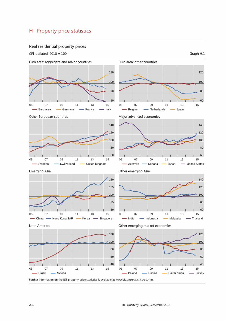
A30 BIS Quarterly Review, September 2015
H Property price statistics
Real residential property prices
CPI-deflated; 2010 = 100 Graph H.1
Euro area: aggregate and major countries Euro area: other countries
Other European countries Major advanced economies
Emerging Asia Other emerging Asia
Latin America Other emerging market economies
Further information on the BIS property price statistics is available at www.bis.org/statistics/pp.htm.
80
90
100
110
05 07 09 11 13 15
Euro area Germany France Italy
60
80
100
120
05 07 09 11 13 15
Belgium Netherlands Spain
60
80
100
120
140
05 07 09 11 13 15
Sweden Switzerland United Kingdom
60
80
100
120
140
05 07 09 11 13 15
Australia Canada Japan United States
50
75
100
125
150
05 07 09 11 13 15
China Hong Kong SAR Korea Singapore
60
80
100
120
140
05 07 09 11 13 15
India Indonesia Malaysia Thailand
40
60
80
100
120
05 07 09 11 13 15
Brazil Mexico
40
60
80
100
120
05 07 09 11 13 15
Poland Russia South Africa Turkey

BIS Quarterly Review, September 2015 A31
I Effective exchange rate statistics
Real effective exchange rates
CPI-based; 1995–2005 = 1001 Graph I.1
Euro area: aggregate and major countries Euro area: other countries
Other European countries Major advanced economies
Emerging Asia Other emerging Asia
Latin America Other emerging market economies
Further information on the BIS effective exchange rate statistics is available at www.bis.org/statistics/eer.htm. 1 An increase indicates an appreciation in the economy’s currency in real terms against a broad basket of currencies.
80
90
100
110
120
05 07 09 11 13 15
Euro area Germany France Italy
80
90
100
110
120
05 07 09 11 13 15
Belgium Netherlands Spain
60
80
100
120
140
05 07 09 11 13 15
Sweden United Kingdom Switzerland
60
80
100
120
140
05 07 09 11 13 15
Australia Canada Japan United States
50
75
100
125
05 07 09 11 13 15
China Hong Kong SAR Korea Singapore
60
80
100
120
05 07 09 11 13 15
India Indonesia Malaysia Thailand
25
50
75
100
125
05 07 09 11 13 15
Argentina Brazil Mexico
50
75
100
125
150
05 07 09 11 13 15
PolandRussia
Saudi ArabiaSouth Africa
Turkey
BIS Quarterly Review, September 2015 B1
Special features in the BIS Quarterly Review
March 2015 The costs of deflations: a historical perspective Claudio Borio, Magdalena Erdem, Andrew Filardo & Boris Hofmann
March 2015 Oil and debt Dietrich Domanski, Jonathan Kearns, Marco Jacopo Lombardi & Hyun Song Shin
March 2015 (Why) Is investment weak? Ryan Banerjee, Jonathan Kearns & Marco Lombardi
March 2015 Financial inclusion - issues for central banks Aaron Mehrotra & James Yetman
March 2015 Shifting tides - market liquidity and market-making in fixed income instruments
Ingo Fender & Ulf Lewrick
December 2014 Currency movements drive reserve composition Robert N McCauley & Tracy Chan
December 2014 Securitisations: tranching concentrates uncertainty Adonis Antoniades & Nikola Tarashev
December 2014 Bank business models Rungporn Roengpitya, Nikola Tarashev & Kostas Tsatsaronis
December 2014 Non-financial corporations from emerging market economies and capital flows
Stefan Avdjiev, Michael Chui & Hyun Song Shin
September 2014 Asset managers in emerging market economies Ken Miyajima & Ilhyock Shim
September 2014 Risks related to EME corporate balance sheets: the role of leverage and currency mismatch
Michael Chui, Ingo Fender &Vladyslav Sushko
September 2014 Cross-border bank lending during the taper tantrum: the role of emerging market fundamentals
Stefan Avdjiev & Előd Takáts
September 2014 Residential property price statistics across the globe Michela Scatigna, Robert Szemere & Kostas Tsatsaronis
BIS Quarterly Review, September 2015 C1
Recent BIS publications1
BIS Working Papers
Higher bank capital requirements and mortgage pricing: evidence from the Countercyclical Capital Buffer (CCB) Christoph Basten and Catherine Koch
How has the CCB affected mortgage pricing after Switzerland became the first country to activate this Basel III macroprudential tool? By analysing a database with several offers per mortgage request, we construct a picture of mortgage supply and demand. We find, first, that the CCB changes the composition of mortgage supply, as relatively capital-constrained and mortgage-specialized banks raise prices more than their competitors do. Second, risk-weighting schemes linked to borrower risk do not amplify the CCB's effect. To conclude, changes in the supply composition suggest that the CCB has achieved its intended effect in shifting mortgages from less resilient to more resilient banks, but stricter capital requirements do not appear to have discouraged less resilient banks from risky mortgage lending.
Global dollar credit and carry trades: a firm-level analysis Valentina Bruno and Hyun Song Shin
We conduct a firm-level analysis of borrowing in US dollars by non-financial corporates from outside the United States. The dataset combines bond issuance data with firm-level financial information. We find that firms with already high cash holdings are more likely to issue US dollar-denominated bonds, and that the proceeds of the bond issue add to cash holdings. The tendency to add cash is more pronounced during periods when the dollar carry trade is more favourable and is prevalent for emerging market firms.
Investor redemptions and fund manager sales of emerging market bonds: how are they related? Jimmy Shek, Ilhyock Shim and Hyun Song Shin
Lending to emerging market economies (EMEs) through bond purchases has surged since 2009. What are the risks of a sudden stop? Bond mutual funds may curtail credit through two channels. The first is redemptions by ultimate investors. The second is additional discretionary sales by fund managers, over and above any sales implied by redemptions. In an empirical analysis of EME bond funds, we find that discretionary sales tend to reinforce the sales due to investor redemptions, and that 100 dollars' worth of bond sales due to investor redemptions is accompanied by roughly 10 dollars' worth of discretionary bond sales. We also find that 100 dollars' worth of EME international bond sales is associated with around 4 dollars' worth of valuation losses. Finally, a 1 percentage point increase in the yield of local currency bonds is associated with a 10% decline in the dollar value of bond holdings.
Bond markets and monetary policy dilemmas for the emerging markets Jhuvesh Sobrun and Philip Turner
Financial conditions in the emerging markets (EMs) have become more dependent on the 'world' long-term interest rate, which has been driven down by monetary policies in the advanced economies - notably Quantitative Easing (QE) - and by several non-monetary factors. This paper analyses some new mechanisms that link global long-term rates to
1 Requests for publications should be addressed to Bank for International Settlements, Press &
Communications, Centralbahnplatz 2, CH-4002 Basel. These publications are also available on the BIS website (www.bis.org).
C2 BIS Quarterly Review, September 2015
monetary policy and to domestic bank lending in the EMs. Understanding these mechanisms could help EM central banks prepare for the exit from QE and higher (and perhaps divergent) policy rates in advanced economies. Although monetary policy in the EMs has continued to be guided by domestic objectives, it has nevertheless lost some traction. Difficult trade-offs now confront central banks.
Macroeconomic effects of banking sector losses across structural models Luca Guerrieri, Matteo Iacoviello, Francisco Covas, John C. Driscoll, Mohammad Jahan-Parvar, Michael Kiley, Albert Queralto and Jae Sim
The macro spillover effects of capital shortfalls in the financial intermediation sector are compared across five dynamic equilibrium models for policy analysis. Although all the models considered share antecedents and a methodological core, each model emphasizes different transmission channels. This approach delivers "model-based confidence intervals" for the real and financial effects of shocks originating in the financial sector. The range of outcomes predicted by the five models is only slightly narrower than confidence intervals produced by simple vector autoregressions.
Macroprudential policies in a commodity exporting economy Andrés González, Franz Hamann and Diego Rodríguez
Colombia is a small open and commodity exporter economy, sensitive to international commodity price fluctuations. During the surge in commodity prices, as income from the resource sector increases total credit expands, boosting demand for tradable and nontradable goods, appreciating the currency and shifting resources from the tradable sector to the non-tradable. Although this adjustment is efficient, the presence of financial frictions in the economy exacerbates the resource allocation process through credit. In this phase, as total credit expands, the appreciation erodes the net worth of the tradable sector and boosts the non-tradable one, and thus credit gets concentrated in that sector. A sudden reversal of commodity prices causes a rapid adjustment of resources in the opposite direction. However, the ability of the tradable sector to absorb the freed resources is limited by its financial capacity. In this scenario, macroprudential policies may help to restrain aggregate credit dynamics and thus prevent or act prudently in anticipation to the effects of large oil price shock reversals. In this work we write a model that accounts for these facts and quantify the role of three policy instruments: short term interest rate, FX intervention and financial regulation. We explore this issues in a DSGE model estimated for the Colombian economy and find that both FX intervention and regulation policies complement the short-term interest rates in smoothing the business cycle by restraining credit, raising market interest rates and smoothing economic activity. However, these additional instruments have undesirable sectoral implications. In particular, the use of these policies implies that credit to the tradable sector dries and becomes more expensive, weakening its financial position, which in turn implies a sharper fall of this sector during the price reversal and a longer recovery. These effects, nonetheless, appear to be quantitatively small according to the estimated model.
Phases of global liquidity, fundamentals news, and the design of macroprudential policy Javier Bianchi and Enrique G Mendoza
The unconventional shocks and non-linear dynamics behind the high volatility of financial markets present a challenge for the implementation of macroprudential policy. This paper introduces two of these unconventional shocks, news shocks about future fundamentals and regime changes in global liquidity, into a quantitative non-linear model of financial crises. The model is then used to examine how these shocks affect the design and effectiveness of optimal macroprudential policy. The results show that both shocks contribute to strengthen the amplification mechanism driving financial crisis dynamics. Macroprudential policy is effective for reducing the likelihood and magnitude of financial crises, but the optimal policy requires significant variation across regimes of global liquidity and realizations of news shocks. Moreover, the effectiveness of the policy improves as the precision of news rises from low levels, but at high levels of precision it becomes less effective (financial crises are less likely, but the optimal policy does not weaken them significantly).
BIS Quarterly Review, September 2015 C3
Credit and macroprudential policy in an emerging economy: a structural model assessment Horacio A Aguirre and Emilio F Blanco
We build a small structural open economy model, augmented to depict the credit market and interest rate spreads (distinguishing by credit to firms and families); monetary policy with sterilized intervention in the foreign exchange market; and macroprudential policy as capital requirements. We estimate the model using Bayesian techniques with quarterly data for Argentina in 2003-2011; it can be extended to other emerging economies, allowing for comparative empirical analysis. Results indicate that shocks to lending rates and spread weigh on macroeconomic variables; likewise, the credit market is affected by macroeconomic shocks. Capital requirements, beyond their strictly prudential role, appear to have contributed to lower volatility of key variables such as output, prices, credit and interest rates. The interaction of monetary policy, foreign exchange intervention and prudential tools appears to be synergic: counting on a larger set of tools helps dampen volatility of both macroeconomic and financial system variables, taking into account the type of shocks faced during the estimation period.
Inflation targeting and financial stability: providing policymakers with relevant information Anders Vredin
Experience from financial crises and central bank policies in the past decade has led to an intensified debate about the relationship between monetary policy and financial stability. Since there is no established theoretical framework for analysing the links between financial stability and monetary policy, it is very difficult to deliver precise recommendations for policy. The primary purpose of this paper is to present suggestions for how risks of financial instability can be taken into account in the information provided to central bank decision makers, despite the considerable uncertainty about the appropriate analytical approach. The paper starts with a discussion of the strategy of "flexible inflation targeting", which, in fact, does not provide any "simple rules" for policymakers. The next section contains a review of theoretical and empirical analyses of links between financial stability and monetary policy. Insights from inflation targeting, and more recent views on the role of financial stability, lead to suggestions regarding the type of information that should be presented to monetary policy decision makers, and how it can be organised, to help them understand the links between financial stability and monetary policy.
Comparative assessment of macroprudential policies Valentina Bruno, Ilhyock Shim and Hyun Song Shin
This paper provides a comparative assessment of the effectiveness of macroprudential policies in 12 Asia-Pacific economies, using comprehensive databases of domestic macroprudential policies and capital flow management (CFM) policies. We find that banking sector CFM polices and bond market CFM policies are effective in slowing down banking inflows and bond inflows, respectively. We also find some evidence of spillover effects of these policies. Finally, regarding the interaction of monetary policy and macroprudential policies, our empirical findings suggest that macroprudential policies are more successful when they complement monetary policy by reinforcing monetary tightening, than when they act in opposite directions.
Basel Committee on Banking Supervision
Basel III: The standardised approach for measuring counterparty credit risk exposures: Frequently asked questions August 2015
The Basel Committee on Banking Supervision has received a number of interpretation questions related to the Standardised Approach for measuring counterparty credit risk (SA-CCR), as published in March 2014 (and revised in April 2014). The SA-CCR will replace both
C4 BIS Quarterly Review, September 2015
current non-internal model approaches, the Current Exposure Method (CEM) and the Standardised Method (SM). To help ensure consistent global implementation of its standards, the Committee has agreed to periodically review frequently asked questions and publish answers along with any technical elaboration of the standards and interpretative guidance that may be necessary. This document presents a set of frequently asked questions that relate to the SA-CCR.
Criteria for identifying simple, transparent and comparable securitisations July 2015
The Basel Committee on Banking Supervision and the International Organization of Securities Commissions (IOSCO) today released final Criteria for identifying simple, transparent and comparable securitisations. The criteria are available on the websites of the Bank for International Settlements and IOSCO.
The purpose of these criteria is to assist in the financial industry's development of simple, transparent and comparable securitisation structures. They are not intended to serve as a substitute for investors' due diligence.
These criteria apply only to term securitisations and are non-exhaustive and non-binding. Additional and/or more detailed criteria may be necessary based on specific needs and applications.
Criteria promoting simplicity refer to the homogeneity of underlying assets with simple characteristics, and a transaction structure that is not overly complex.
Criteria on transparency provide investors with sufficient information on the underlying assets, the structure of the transaction and the parties involved in the transaction, thereby promoting a more thorough understanding of the risks involved. The form in which the information is available should not hinder transparency, but instead it should support investors in their assessment.
Criteria promoting comparability could assist investors in their understanding of such investments and enable more straightforward comparison between securitisation products within an asset class.
General guide to account opening - consultative document July 2015
The Basel Committee on Banking Supervision has today issued for public consultation a revised version of the General guide to account opening, which was first published in February 2003.
Most bank-customer relationships start with an account opening procedure. The customer information collected and verified at this stage is crucial in order for the bank to fulfil its obligations under anti-money laundering and counter-financing of terrorism (AML/CFT) rules. As a result, banks' policies and procedures for account opening must fully reflect applicable AML/CFT legislation.
When finalised, the proposed revised version of the General guide to account opening will be added as an annex to the Committee's Sound management of risks related to money laundering and financing of terrorism, published in January 2014. The proposed guide expands on, and should be read in conjunction with, the 2014 guidelines.
The proposed guide is in no way intended to strengthen, weaken or otherwise modify the existing Financial Action Task Force (FATF) standards. Rather, it aims to support banks in implementing the FATF standards and guidance, which requires the adoption of specific policies and procedures, in particular on account opening.
The Committee welcomes comments on this consultative document. Comments should be uploaded here by Thursday 22 October 2015 or they may be sent by post to: Secretariat of the Basel Committee on Banking Supervision, Bank for International Settlements, CH-4002 Basel, Switzerland. All comments will be published on the website of the Bank for International Settlements unless a respondent requests confidential treatment.

BIS Quarterly Review, September 2015 C5
Guidelines for identifying and dealing with weak banks July 2015
The Basel Committee on Banking Supervision today published the final Guidelines for identifying and dealing with weak banks.
Weak banks are a worldwide phenomenon. They pose a continuing challenge for bank supervisors and resolution authorities in all countries, regardless of the political structure, financial system and level of economic and technical development. All bank supervisors should be prepared to mitigate the incidence of weak banks and deal with them when they occur.
In the light of the significant post-crisis developments in financial markets and the regulatory landscape, the Committee has updated its 2002 Supervisory guidance on dealing with weak banks. Key changes include:
- emphasising the need for early intervention and the use of recovery and resolution tools, and updating supervisory communication policies for distressed banks;
- providing further guidance for improving supervisory processes, such as incorporating macroprudential assessments, stress testing and business model analysis, and reinforcing the importance of sound corporate governance at banks;
- highlighting the issues of liquidity shortfalls, excessive risk concentrations, misaligned compensation and inadequate risk management; and
- expanding guidelines for information-sharing and cooperation among relevant authorities.
Part I of the report discusses the underlying supervisory preconditions for dealing with weak banks and techniques that will allow the supervisor to identify problems. These phases include preparatory work on recovery and resolution issues. Part II concerns the corrective measures available to turn around a weak bank and, for resolution authorities, tools for dealing with failing or failed banks.
A consultative version of this paper was published for comment in June 2014. The guidelines published today supersede the Committee's 2002 guidance on the topic.
French translation to be published soon
Progress report on the implementation of principles for effective supervisory colleges July 2015
The Basel Committee on Banking Supervision has today issued a Progress report on the implementation of principles for effective supervisory colleges.
The Basel Committee first published good practice principles on supervisory colleges in 2010 and issued a revised set of Principles for effective supervisory colleges in 2014. The Committee continues to monitor the implementation of the principles and to review the effectiveness of colleges. This progress report sets out the detailed findings, based on the monitoring initiatives undertaken by the Basel Committee, and highlights challenges faced by supervisors in running effective supervisory colleges as well as the practical approaches taken to address them.
The key findings of the colleges' monitoring can be summarised as follows:
While there is room for improvement in several areas, the broad sense of supervisors - from both a home and a host perspective - is that the functioning of supervisory colleges has continued to improve and that supervisors have made considerable advances in implementing the college principles.
Colleges play a key role in assisting supervisors by giving both home and host supervisors a comprehensive view of risks and vulnerabilities to a firm and identifying emerging risks on a timely basis.
Colleges have evolved into key forums for rigorous discussion of broader issues that enhance supervision of global firms and contribute to the planning of supervisory assessments.
C6 BIS Quarterly Review, September 2015
A wide range of college structures has been developed by home supervisors to reflect the differing size, complexity and global reach of internationally active banks, and home supervisors have a greater sensitivity to host supervisor concerns in developing criteria for college membership.
Legal and institutional arrangements are important contributors to successful colleges and have been enhanced in recent years, but trust and mutual understanding among members are at least as important.
The collaborative work among college members contributes to improving the effectiveness of the oversight of cross-border banking groups.
While supervisors report that interaction with firms has improved in supervisory colleges, particularly in terms of a higher-quality engagement with management, many firms have indicated that they would like to receive more feedback on college discussions.
Although some progress has been made as regards the role of colleges in crisis preparedness, this principle has also been cited as the area with the most implementation challenges, in part because crisis management groups have assumed some of the responsibilities formerly undertaken in supervisory colleges.
Corporate governance principles for banks July 2015
The Basel Effective corporate governance is critical to the proper functioning of the banking sector and the economy as a whole. While there is no single approach to good corporate governance, the Basel Committee's revised principles provide a framework within which banks and supervisors should operate to achieve robust and transparent risk management and decision-making and, in doing so, promote public confidence and uphold the safety and soundness of the banking system.
The Committee's revised set of principles supersedes guidance published by the Committee in 2010. The revised guidance emphasises the critical importance of effective corporate governance for the safe and sound functioning of banks. It stresses the importance of risk governance as part of a bank's overall corporate governance framework and promotes the value of strong boards and board committees together with effective control functions. More specifically, the revised principles:
- expand the guidance on the role of the board of directors in overseeing the implementation of effective risk management systems;
- emphasise the importance of the board's collective competence as well as the obligation of individual board members to dedicate sufficient time to their mandates and to keep abreast of developments in banking;
- strengthen the guidance on risk governance, including the risk management roles played by business units, risk management teams, and internal audit and control functions (the three lines of defence), as well as underline the importance of a sound risk culture to drive risk management within a bank;
- provide guidance for bank supervisors in evaluating the processes used by banks to select board members and senior management; and
- recognise that compensation systems form a key component of the governance and incentive structure through which the board and senior management of a bank convey acceptable risk-taking behaviour and reinforce the bank's operating and risk culture.
A consultative version of the Corporate governance principles for banks was published in October 2014. The Basel Committee wishes to thank all those who contributed time and effort to express their views during the consultation process.
BIS Quarterly Review, September 2015 C7
Frequently asked questions on the Basel III leverage ratio framework July 2015
In January 2014, the Basel Committee on Banking Supervision published the Basel III leverage ratio framework and disclosure requirements together with the public disclosure requirements applicable as of 1 January 2015. To promote consistent global implementation of those requirements, the Committee has agreed to periodically review frequently asked questions (FAQs) and publish answers along with any technical elaboration of the standards text and interpretative guidance that may be necessary.
The document published today sets out the first and second set of FAQs that relate to the Basel III leverage ratio framework. The questions and answers are grouped according to different relevant areas:
- (i) criteria for the recognition of cash variation margin associated with derivative exposures;
- (ii) centrally cleared client derivative exposures;
- (iii) exposures and netting of securities financing transactions (SFTs);
- (iv) the treatment of netting of SFTs and derivatives under a cross-product netting agreement;
- (v) the exposure measure under the additional treatment for credit derivatives; and
- (vi) the treatment of long settlement transactions and failed trades.
Report on the impact and accountability of banking supervision July 2015
The Report on impact and accountability of banking supervision presents a range-of-practice study on how supervisors around the world define and evaluate the impact of their policies and actions, manage against that impact and then account for it to their external stakeholders.
In response to the global financial crisis, standard-setting bodies and national authorities initiated a broad overhaul of the regulatory framework. The implementation of Basel III makes a necessary and important contribution to strengthening regulation and increasing the resilience of banks. However, regulatory reforms alone cannot assure the soundness and stability of financial institutions; they must be supported by effective supervision.
In recent years, supervisors have revised and strengthened their strategy and practice. Supervision has become more comprehensive and intrusive, taking additional dimensions of a bank's business into account. Supervisors have also taken steps to gain more insight into the impact of their activities.
Measuring the impact of supervision is a relatively new area. Jurisdictions have nevertheless developed various practices to show how their activities contribute to the soundness and stability of financial institutions and of the financial system. That said, no analysis is straightforward, because supervisors have to deal with methodological challenges and because there is no unique method or indicator that can be singled out in response to these challenges. Thus, current experience must be discussed while practices are still evolving.
Finally, the report shows how a well-designed system of accountability can support operational independence and enhance transparency, while safeguarding confidential, institution-specific information.
Review of the Credit Valuation Adjustment (CVA) risk framework - consultative document July 2015
A Review of the Credit Valuation Adjustment Risk Framework is being undertaken by the Basel Committee. The objectives of the review are to (i) ensure that all important drivers of credit valuation adjustment (CVA) risk and CVA hedges are covered in the Basel regulatory

C8 BIS Quarterly Review, September 2015
capital standard; (ii) align the capital standard with the fair value measurement of CVA employed under various accounting regimes; and (iii) ensure consistency with the proposed revisions to the market risk framework under the Basel Committee's Fundamental review of the trading book.
The Basel III capital framework already establishes a minimum capital charge to capture the potential mark-to-market losses faced by a bank from the deterioration in a counterparty's creditworthiness. This capital treatment addresses any variability in CVA that arises due to changes in credit spreads but does not take account of variability arising from daily changes in market risk factors (ie account exposure variability).
This consultative paper envisages a CVA risk framework that takes into account the market risk exposure component of CVA along with its associated hedges. The regulatory capital requirement for CVA risk would be based on exposure models that banks also use to determine their accounting CVA, subject to conditions intended to reduce potential variability due to risk-weighted asset (RWA) calculations or remaining discrepancies in financial reporting practices across banks and jurisdictions.
For a broad range of internationally active banks, accounting CVA is fair-valued through the profit and loss (P&L) account and is sensitive to the same risk factors as instruments held in the trading book. The consultative paper therefore proposes an internal models approach and a standardised approach for CVA risk that have been adapted from the revised market risk framework under the Committee's Fundamental review of the trading book. A basic approach for CVA risk is also proposed for banks that are less likely to regularly compute CVA sensitivities to a large set of market risk factors, owing to the nature of their trading operations.
Net Stable Funding Ratio disclosure standards June 2015
Disclosure requirements for the Net Stable Funding Ratio ("NSFR") have been developed to improve the transparency of regulatory funding requirements, reinforce the Principles for sound liquidity risk management and supervision, strengthen market discipline, and reduce uncertainty in the markets as the NSFR standard is implemented.
Similar to the LCR disclosure framework, and to promote the consistency and usability of disclosures related to the NSFR, internationally active banks in all Basel Committee member jurisdictions will be required to publish their NSFRs according to a common template. This NSFR disclosure template includes the major categories of sources and uses of stable funding.
In parallel with the implementation of the NSFR standard, supervisors will give effect to these disclosure requirements, and banks will be required to comply with them from the date of the first reporting period after 1 January 2018.
Interest rate risk in the banking book - consultative document June 2015
The consultative document on the risk management, capital treatment and supervision of interest rate risk in the banking book (IRRBB) expands upon and is intended to ultimately replace the Basel Committee's 2004 Principles for the management and supervision of interest rate risk.
The Committee's review of the regulatory treatment of interest rate risk in the banking book is motivated by two objectives: First, to help ensure that banks have appropriate capital to cover potential losses from exposures to changes in interest rates. This is particularly important in the light of the current exceptionally low interest rate environment in many jurisdictions. Second, to limit capital arbitrage between the trading book and the banking book, as well as between banking book portfolios that are subject to different accounting treatments. The paper presents two options for the capital treatment of interest rate risk in the banking book:
- (i) the adoption of a uniformly applied Pillar 1 measure for calculating minimum capital requirements, which would have the benefit of promoting greater

BIS Quarterly Review, September 2015 C9
consistency, transparency and comparability, thereby promoting market confidence in banks' capital adequacy and a level playing field internationally; and
- (ii) a Pillar 2 option, which includes quantitative disclosure of interest rate risk in the banking book based upon the proposed Pillar 1 approach, which would better accommodate differing market conditions and risk management practices across jurisdictions.
Developments in credit risk management across sectors: current practices and recommendations June 2015
The report provides insight into the current supervisory framework around credit risk, the state of credit risk management at firms and implications for the supervisory and regulatory treatments of credit risk.
It is based on a survey that the Joint Forum conducted with supervisors and firms in the banking, securities and insurance sectors globally in order to understand the current state of credit risk management given the significant market and regulatory changes since the 2008 financial crisis. Fifteen supervisors and 23 firms from Europe, North America and Asia responded to the survey.
The report updates previous Joint Forum work on this topic, particularly Regulatory and market differences: issues and observations (2006), and used the date of that report as the benchmark when analysing changes in the field of credit risk management.
The report includes the following recommendations for consideration by supervisors.
Recommendation 1: Supervisors should be cautious against over-reliance on internal models for credit risk management and regulatory capital. Where appropriate, simple measures could be evaluated in conjunction with sophisticated modelling to provide a more complete picture.
Recommendation 2: With the current low interest rate environment possibly generating a "search for yield" through a variety of mechanisms, supervisors should be cognisant of the growth of such risk-taking behaviours and the resulting need for firms to have appropriate risk management processes.
Recommendation 3: Supervisors should be aware of the growing need for high-quality liquid collateral to meet margin requirements for OTC derivatives sectors, and if any issues arise in this regard they should respond appropriately. The Joint Forum's Parent Committees (BCBS, IAIS and IOSCO) should consider taking appropriate steps to promote the monitoring and evaluation of the availability of such collateral in their future work while also considering the objective of reducing systemic risk and promoting central clearing through collateralisation of counterparty credit risk exposures that stems from non-centrally cleared OTC derivatives.
Recommendation 4: Supervisors should consider whether firms are accurately capturing central counterparty exposures as part of their credit risk management.
Committee on the Global Financial System
Regulatory change and monetary policy May 2015
Financial regulation is evolving, as policymakers seek to strengthen the financial system in order to make it more robust and resilient. Changes in the regulatory environment are likely to have an impact on financial system structure and on the behaviour of financial intermediaries that central banks will need to take into account in how they implement monetary policy.
Against this background, this report assesses the combined impact of key new regulations on monetary policy. It is based on information from a range of sources, including central bank
C10 BIS Quarterly Review, September 2015
case studies as well as structured interviews with private sector market participants. It argues that the likely impacts of the new financial regulations on financial institutions and markets should have only limited and manageable effects on monetary policy operations and transmission. Hence, as necessary, central banks should be able to make adjustments within their existing policy frameworks and in ways that preserve policy effectiveness. These adjustments will tend to differ across jurisdictions according to the financial systems and policy frameworks in place. Specific implications, and examples of potential policy responses, are set out and elaborated in more detail in the report.
Committee on Payments and Market Infrastructures
Harmonisation of key OTC derivatives data elements (other than UTI and UPI) – first batch, consultative report issued by CPMI-IOSCO September 2015
G20 Leaders agreed in 2009 that all over-the-counter (OTC) derivatives contracts should be reported to trade repositories (TRs) as part of their commitment to reform OTC derivatives markets in order to improve transparency, mitigate systemic risk and protect against market abuse. Aggregation of the data reported across TRs is necessary to help ensure that authorities are able to obtain a comprehensive view of the OTC derivatives market and activity.
Following the 2014 FSB Feasibility study on approaches to aggregate OTC derivatives data, the FSB asked the CPMI and IOSCO to develop global guidance on the harmonisation of data elements reported to TRs and important for the aggregation of data by authorities, including Unique Transaction Identifier (UTIs) and Unique Product Identifiers (UPIs).
This consultative report is one part of the CPMI-IOSCO Harmonisation Group's response to its mandate. It focuses on a first batch of key data elements (other than UTI and UPI) that are considered important for consistent and meaningful aggregation on a global basis.
The report seeks comments on these proposals as well as responses to the general and specific questions by 9 October 2015, to be sent to both the CPMI secretariat and the IOSCO secretariat.
Besides this consultative report, the CPMI and IOSCO have already issued a consultative report on Harmonisation of the Unique Transaction Identifier, and plan to issue consultative reports on global UPIs and on further batches of key data elements (other than UTI and UPI) in the coming months.
Harmonisation of the Unique Transaction Identifier - consultative report August 2015
G20 Leaders agreed in 2009 that all over-the-counter (OTC) derivatives contracts should be reported to trade repositories (TRs) as part of their commitment to reform OTC derivatives markets in order to improve transparency, mitigate systemic risk and protect against market abuse. Aggregation of the data reported across TRs is necessary to help ensure that authorities are able to obtain a comprehensive view of the OTC derivatives market and activity.
Following the 2014 FSB Feasibility study on approaches to aggregate OTC derivatives data, the FSB asked the CPMI and IOSCO to develop global guidance on the harmonisation of data elements reported to TRs and important for the aggregation of data by authorities, including Unique Transaction Identifier (UTIs) and Unique Product Identifiers (UPIs).
This consultative report is one part of the CPMI-IOSCO Harmonisation Group's response to its mandate. It focuses on the harmonised global UTI, whose purpose is to uniquely identify each OTC derivative transaction required by authorities to be reported to TRs. The final objective is to produce clear guidance as to UTI definition, format and usage that meets the
BIS Quarterly Review, September 2015 C11
needs of UTI users, is global in scale, and is jurisdiction-agnostic, thus enabling the consistent global aggregation of OTC derivatives transaction data.
Application of the "Principles for financial market infrastructures" to central bank FMIs August 2015
Collateral The Committee on Payments and Market Infrastructures (CPMI) and the International Organization of Securities Commissions (IOSCO) have issued this short note providing guidance on how the Principles for financial market infrastructures (PFMI) applies to financial market infrastructures that are owned and operated by central banks. It develops what is said in the PFMI itself and further clarifies the interaction between the PFMI and central bank policies.
Implementation monitoring of PFMIs: Second update to Level 1 assessment report June 2015
The Committee on Payments and Market Infrastructures (CPMI) and the International Organization of Securities Commissions (IOSCO) continue to closely monitor the implementation of the Principles for financial market infrastructures (PFMIs). The PFMIs are international standards for payment, clearing and settlement systems, and trade repositories. They are designed to ensure that the infrastructure supporting global financial markets is robust and well placed to withstand financial shocks.
This report provides jurisdictions' updated self-assessments on progress towards adopting the legislation, regulations and other policies that will enable them to implement the 24 Principles for FMIs and four of the five Responsibilities for authorities included in the PFMIs. It shows that good progress has been made by the 28 participating jurisdictions since the previous update in May 2014. In particular, the gap in the progress on implementation measures applicable to central securities depositories and securities settlement systems vis-a-vis other FMI types has now been closed. The next update of the Level 1 assessments will be conducted in 2016.
Speeches
On the centrality of the current account in international economics
Keynote speech by Mr Claudio Borio, Head of Monetary and Economic Department of the BIS, at the ECB-Central Bank of Turkey conference "Balanced and sustainable growth - operationalising the G20 framework", Frankfurt, 28 August 2015.
The current account occupies a central position in international economics and policy debates. Indeed, in G20 policy debates the term "global imbalances" is treated as almost synonymous with "current account imbalances". Current account imbalances do matter and they can be a problem. But this speech argues that this centrality is not that helpful in understanding how the global economy works, especially in a world of free and huge capital flows. And it may even lead to the wrong policy prescriptions, including not paying sufficient attention to potentially more disruptive financial imbalances. A key reason is that, analytically, the current account is asked to shed light on issues for which it is ill-suited, such as the amount of financing a country gets from, or provides to, others, the direction of that financing (who lends to whom) and financial instability.
Credit booms and credit busts
Interview with Claudio Borio, Head of the Monetary and Economic Department, and the Institute for New Economic Thinking (INET), 10 July 2015
There is now a growing consensus among policymakers and academics that a key element to improve safeguards against financial instability is to strengthen the "macroprudential" orientation of regulatory and supervisory frameworks. Claudio Borio speaks with INET's Marshall Auerback on this topic.
C12 BIS Quarterly Review, September 2015
The role of the CPMI as part of the Basel Process
Presentation Keynote speech by Mr Jaime Caruana, General Manager of the BIS, at the CPMI 25th Anniversary Conference, Basel, 30 June 2015.
Today we are celebrating a birthday, a happy event. At a still youthful 25, the CPMI does not yet have to worry about the problems of old age. Congratulations are therefore in order. So let me begin by complimenting the Committee on one fundamental accomplishment that we know but is perhaps not enough publicly recognised.
The crisis that erupted in 2008 revealed the financial sector's many shortcomings. But the infrastructure that supports payment, clearing and settlement was not among them. On the contrary, the various financial market infrastructures - or FMIs - withstood the battering they received while the markets around them were in turmoil, and continued to function smoothly, with little or no damage.
If in 2008, the market infrastructure had been in the same state as it was back in 1990, then the outcome could have been rather different. It has been said many times before, but it bears repeating: FMIs are fundamental to the ability of markets to work. A weak infrastructure can turn a small crisis into a huge one. The fact that the infrastructure was strong enough in 2008 is in large part thanks to the many efforts of this committee since its inception. The introduction of improvements such as real-time gross settlement (RTGS) for payments, delivery-versus-payment (DVP) for securities, and payment-versus-payment (PVP) for foreign exchange has made a real and substantial difference. So, congratulations!
In the rest of my remarks, I shall first highlight three snapshots from the Committee's history, corresponding to the three sessions of this conference. Then, I shall talk about how the Committee has been working in the context of what we at the BIS call the Basel Process. Finally, I shall share with you a few thoughts on one of the outcomes of the financial crisis, namely the growing role of centralised counterparties or CCPs.
The history of the CPMI
First, some history and its relation to the three sessions of this conference. To preserve the chronology of the actual events, I will take the sessions in a different order, starting with Session 2.
Session 2 is about the resilience, recovery and resolution of FMIs. As I mentioned earlier, one of the CPMI's most significant contributions is the promotion of PVP as a safer way to settle foreign exchange. Many of you in this audience would know that the history behind this goes back to 1974 and the so-called Herstatt crisis. The direct consequence of that for us here in Basel was in fact the creation of the Basel Committee on Banking Supervision (BCBS), not the Committee on Payment and Settlement Systems (CPSS). It was only some years later that people recognised the need for a more specialised group to work on settlement issues. Nevertheless, despite its later start, the CPSS embraced FX settlement as one of its initial, defining projectstogether to produce the BCBS's 2013 Supervisory guidance for managing risks associated with the settlement of foreign exchange transactions. In the coming years, this cooperation will bear fruit as risks are better recognised and addressed.
Session 3 of this conference is about disruptive innovations. Here I'd like to refer to what might be called the prehistory of the Committee. In a way, the Committee can be considered to be not 25 but 35 years old, given that its predecessor, the Group of Experts on Payment Systems, was set up in 1980. What led to the formation of that group was a major innovation that, as it happened, was highly disruptive, namely the conversion of paper-based large-value payment systems to electronic ones. This was a change driven by technology. And it occurred at a time when financial markets were starting to grow rapidly in size. The combination - new technology and bigger markets - led central banks to wonder, quite rightly, what the risk implications might be. And it turned out that what was relatively harmless when payments were slow and small became potentially disastrous when they were fast and large. Back in those days, banks received information about incoming payments in real time during the day and credited their customers' accounts immediately based on that information. But settlement between banks took place only at the end of the day. The result: large amounts of

BIS Quarterly Review, September 2015 C13
intraday interbank credit, that was hardly visible, understood or controlled by the banks. This development led to what was, thankfully, only a brief era of electronic large-value deferred settlement arrangements, before real-time settlement came to dominate.
Session 1 is about the evolution of standard setting. For many years, some of the most influential norms in the payment and settlement area came in the report that was, in effect, the father of the CPSS - that is, the Lamfalussy report of 1990, published just as the CPSS was created. This report was a key response both to that disruptive innovation of electronic deferred settlement and to the problem of Herstatt. The first reports issued by the CPSS itself were statistical in nature, very different from standard setting. But soon thereafter, the Committee started producing a wide range of normative statements. The terms used to describe these statements varied, but curiously, the term "standards" was rare. It appeared in the 1990 Lamfalussy report, and then again this year when "disclosure standards" for CCPs were published. But in between, the Committee used a bewildering variety of terms: principles, core principles, general principles, recommended actions, recommendations, responsibilities, propositions, and guidelines. In the last couple years, under the initiative of Paul Tucker and concluded under Benoît Cœuré, the CPSS's international standard -setting role was explicitly confirmed by its governance bodies: the Economic Consultative Committee (ECC) and the Global Economy Meeting. The CPSS became the CPMI.
The Basel Process
Now let me turn to the second part of my remarks. In this birthday event, a lot is bound to be said about what the Committee has accomplished to date. These accomplishments depend not only on the hard work of successive generations of committee chairmen and members as well as secretariat staff, but also the Committee's cooperation with others, in particular, in the context of the Basel Process.
We use the term Basel Process to refer to the active cooperation among the committees and organisations hosted by the BIS and their interaction with the BIS to support their work in prudential standard setting or, more generally, in the pursuit of financial stability. Currently, six committees and three associations find their homes at the BIS. The process is based on three key features: synergies, flexibility and openness, and support from the BIS itself. Each of these is relevant in the case of the CPMI.
First, on synergies. The physical proximity of the BIS-based committees and associations facilitates contact and exchange of ideas across groups. In addition, these groups share a common goal of promoting financial stability. It therefore makes sense for them to work together. Good infrastructure is only valuable if it is used, and used appropriately. It is therefore not surprising that there has been a long history of cooperation between the CPMI and the BCBS, in particular. Of course, the CPMI and IOSCO also have a close relationship - so much so that, over the past five years, roughly half of the CPMI's publications have been joint publications with IOSCO. Indeed, in an increasingly complex financial system, no committee or group can expect to work by itself in isolation. Cooperation across disciplines and across jurisdictions is essential - as is taking a systemic approach to financial stability. The CPMI should be commended for extending this cooperative spirit and systemic view globally.
Another feature of the Basel Process is flexibility and openness. The BIS-based committees are by design limited in size. This kind of setup makes discussion, coordination and cooperation easier, with corresponding benefits to the quality of the output. At the same time, this output can be much larger than the size of the committees would suggest, as they can leverage the expertise of the international community of central bankers, financial regulators and supervisors, and other public authorities. The committees' output needs legitimacy if it is to be effective. International standards are not laws. Jurisdictions have to agree to implement them, and that is more likely to happen if the standards are respected not just for the quality of the product but also for the nature of the process by which they are produced. In the latter respect, governance is crucial. An important change in this regard for the CPMI - and some of its sister committees - came in 2009, when the Committee started to report not to the G10 Governors but to the ECC and the Global Economy Meeting, which consists of the Governors of 30 BIS member central banks. Accompanying this change was an expansion of the membership of the Committee itself. Both changes have made the
C14 BIS Quarterly Review, September 2015
Committee more representative of the world economy and its financial centres. There was indeed some concern at the time that an expanded membership might make the Committee unwieldy and thus less effective. Happily, that proved to be a misplaced concern, and the friendly and cooperative spirit of the committee is undiminished.
Finally, the third key feature of the Basel Process is support from the BIS itself. The work of the Basel-based groups is informed by the BIS's research and analysis, its work in international financial statistics and the practical experience it gains from its banking activities. Given the very specialised - or some may even say esoteric - nature of the CPMI's work, most of the interaction has been in the form of BIS statistical support, whether for the Committee's regular statistics - which are still the most downloaded CPMI publications - or for ad hoc topics. Some of these ad hoc projects, such as the 1998 FX survey, were very large-scale and would have been difficult to carry out if the Committee had not collaborated with BIS colleagues in the statistics area.
Into the limelight?
Let me now proceed to the final part of my remarks and look to the future. I referred a moment ago to the perception that CPMI work was technical or even esoteric. That perception can have certain advantages. By focusing on technical issues, Committee members can have relatively cool-headed discussions of difficult topics without being too much impinged upon by political considerations. The mainly technical and not so political nature of the discussions also means that the CPMI has traditionally been shielded from the limelight - in stark contrast to the BCBS, for example.
But the financial crisis may have changed this to some extent. As I mentioned earlier, by and large, FMIs performed well during the crisis. Nevertheless, there were lessons to be learnt - for both the private and public sectors - and sounder standards were proven necessary. Without the vast public sector support seen during the crisis, for instance, there would surely have been more failures of banks, and thus more stress on infrastructures. FMIs might not have withstood such added stress with so little damage. And as noted earlier, FMIs have to be robust even in the worst crises.
In this respect, let me share a few thoughts on the growing role of CCPs. As you know, one important element of the regulatory agenda to reduce systemic risk is to encourage the use of CCPs, not least by making the clearing of standardised OTC derivatives mandatory.
The benefits of CCPs are qualitatively different from the benefits of the other major infrastructure changes I have mentioned. Mechanisms such as RTGS, DVP and PVP remove what are, in effect, unnecessary frictions in the settlement process. By and large, they remove risks that were due only to poor design or poor processes. And arguably, the safer infrastructure was introduced even before banks themselves fully realised what those risks were.
But this is not the case with clearing, where banks are well aware of counterparty risk. Moreover, such risk is not merely an unnecessary friction of settlement; it is an inevitable feature of trading. CCPs can do a lot both to reduce that risk, for example through multilateral netting, and to ensure that the residual risk is managed effectively by the market as a whole. That is why CCPs are potentially so valuable. However, as CCPs have grown in prominence - and as there is greater awareness of the responsibility put on them to manage risk effectively - there have also been legitimate questions about whether CCPs are safe enough to cope with that responsibility. At the same time, competition between CCPs has brought significant political elements into the picture.
Against this background, the CPMI may be moving into the limelight. Such a move may be uncomfortable at times. But, at least on this occasion, it is helpful. It is helping us to ask the right questions and find the right answers. The substance of this issue will, no doubt, be discussed in the second session, so I will not say much here. But I will note the following: it is certainly important that high standards are set for CCP safety, but it is not enough. CCPs also need to be supervised and overseen with rigour. Supervisors and overseers need to make sure that CCP managers are internalising the economic and social costs that instability in the infrastructure can entail. In other words, competent authorities need to do this work with a
BIS Quarterly Review, September 2015 C15
systemic view. Again, good infrastructure is only valuable if it is used, and used properly. CCPs cannot magically remove all the risk. Ultimately, banks themselves must be responsible for the risks they take and manage them effectively. CCPs can be an enormous help, but they are by no means a complete solution.
Conclusion
Now let me conclude by simply saying, once again, happy birthday CPMI. And thank you for the great work you have done, and will no doubt continue to do. Thanks also to Benoît, the Secretariat and Klaus Löber, former members and former chairs, Bill and Paul, who are here today.
General Manager's speech: Taking a longer-term perspective
Speech and presentation of the key messages of the BIS Annual Report delivered by Mr Jaime Caruana, General Manager of the BIS, on the occasion of the Bank's Annual General Meeting, Basel, 28 June 2015.
The speech highlights four observations from the Annual Report. All of them derive from taking a longer-term perspective that highlights the role of financial and global factors. Persistent unusually low interest rates are not inevitable: they should not be accepted as the new normal. It is important to recognise the long-term damage that financial booms and busts do to productivity growth, mainly by misallocating resources. Persistent very low rates pose risks to the financial sector's strength. And the blind spot of the current international monetary and financial system is its inability to constrain the build-up and transmission of financial imbalances. Fully developing this longer-term perspective and translating its insights into policymaking will require deeper analysis and closer international cooperation.
Persistent unusually low interest rates. Why? What consequences?
Presentation on the BIS Annual Report by Claudio Borio, Head of the Monetary and Economic Department, on the occasion of the Bank's Annual General Meeting, Basel, 28 June 2015.
The presentation develops a core theme of the Annual Report. It argues that persistent unusually low interest rates are not necessarily "equilibrium" or "natural rates", conducive to sustainable and balanced global expansion. The dominant analytical perspective defines equilibrium rates too narrowly in terms of the behaviour of inflation. As a result, it does not properly integrate financial instability and its large output costs, notably through the impact of resource misallocations on productivity growth. The broader perspective proposed in the Report casts new light on the long-term decline in real interest rates, helps us better understand possible risks for the global economy and calls for a role to be assigned to monetary policy alongside macroprudential policy in preserving financial stability.
Three BIS research themes in the Annual Report
Presentation on the BIS Annual Report by Hyun Song Shin, Economic Adviser and Head of Research, on the occasion of the Bank's Annual General Meeting, Basel, 28 June 2015
The Annual Report reflects the three research themes that have guided our work at the BIS: characteristics of financial intermediation; global liquidity and spillovers; and monetary and financial stability policy frameworks. This presentation describes how findings from research on these themes inform recent changes in long-term interest rates, exchange rates and financial conditions more broadly in the global financial system.