BIPEDAL ROBOTIC WALKING ON FLAT-GROUND, UP-SLOPE AND ROUGH

TERRAIN WITH HUMAN-INSPIRED HYBRID ZERO DYNAMICS

A Thesis

by

SHISHIR NADUBETTU YADUKUMAR

Submitted to the Office of Graduate Studies ofTexas A&M University

in partial fulfillment of the requirements for the degree of

MASTER OF SCIENCE

Approved by:

Chair of Committee, Aaron D. AmesCommittee Members, Shankar P. Bhattacharyya

Mehrdad EhsaniIgor Zelenko

Head of Department, Ohannes Eknoyan

December 2012

Major Subject: Electrical and Computer Engineering

Copyright 2012 Shishir Nadubettu Yadukumar

ABSTRACT

The thesis shows how to achieve bipedal robotic walking on flat-ground, up-slope and

rough terrain by using Human-Inspired control. We begin by considering human walking

data and find outputs (or virtual constraints) that, when calculated from the human data,

are described by simple functions of time (termed canonical walking functions). Formally,

we construct a torque controller, through model inversion, that drives the outputs of the

robot to the outputs of the human as represented by the canonical walking function; while

these functions fit the human data well, they do not apriori guarantee robotic walking (due

to do the physical differences between humans and robots). An optimization problem is

presented that determines the best fit of the canonical walking function to the human data,

while guaranteeing walking for a specific bipedal robot; in addition, constraints can be

added that guarantee physically realizable walking. We consider a physical bipedal robot,

AMBER, and considering the special property of the motors used in the robot, i.e., low

leakage inductance, we approximate the motor model and use the formal controllers that

satisfy the constraints and translate into an efficient voltage-based controller that can be

directly implemented on AMBER. The end result is walking on flat-ground and up-slope

which is not just human-like, but also amazingly robust. Having obtained walking on

specific well defined terrains separately, rough terrain walking is achieved by dynamically

changing the extended canonical walking functions (ECWF) that the robot outputs should

track at every step. The state of the robot, after every non-stance foot strike, is actively

sensed and the new CWF is constructed to ensure Hybrid Zero Dynamics is respected in

the next step. Finally, the technique developed is tried on different terrains in simulation

and in AMBER showing how the walking gait morphs depending on the terrain.

ii

ACKNOWLEDGMENTS

I would like to thank my committee chair, Dr. Aaron Ames, and my committee

members, Dr. Bhattacharyya, Dr. Ehsani and Dr. Zelenko for their guidance and sup-

port throughout the course of this research. Thanks also go to my friends and colleagues

and the department faculty and staff for making my time at Texas A&M University a great

experience. I also want to extend my gratitude to the National Science Foundation, Nor-

mann Hackerman Advanced Research Program who funded my research and also National

Instruments who provided the necessary hardware and software.

Finally, thanks to my mother and father for their constant encouragement.

iii

TABLE OF CONTENTS

CHAPTER Page

I INTRODUCTION . . . . . . . . . . . . . . . . . . . . . . . . . . 1

II BIPEDAL ROBOTIC MODEL . . . . . . . . . . . . . . . . . . . . 4

II.1. Biped Description . . . . . . . . . . . . . . . . . . . . . . 4

III HUMAN-INSPIRED CONTROL . . . . . . . . . . . . . . . . . . 9

III.1. Human-Inspired Functions . . . . . . . . . . . . . . . . . . 9III.2. Human-Inspired Controller . . . . . . . . . . . . . . . . . . 12III.3. Human-Inspired Hybrid Zero Dynamics (HZD) . . . . . . . 13III.4. Optimization Theorem . . . . . . . . . . . . . . . . . . . . 15

IV FLAT-GROUND AND UP-SLOPE WALKING IN AMBER . . . . . 20

IV.1. Human-Inspired Voltage Control . . . . . . . . . . . . . . . 20IV.2. Simulation and Experimental Results . . . . . . . . . . . . 22

IV.2.1. Flat-ground walking . . . . . . . . . . . . . . . . . . . 22IV.2.2. Walking on a slope . . . . . . . . . . . . . . . . . . . 23

V WALKING ON ROUGH TERRAIN . . . . . . . . . . . . . . . . . 31

V.1. Extended Canonical Walking Function (ECWF) andIntermediate Motion Transitions (IMT) . . . . . . . . . . . 31

V.2. Experimental Implementation of IMT . . . . . . . . . . . . 38

VI CONCLUSIONS . . . . . . . . . . . . . . . . . . . . . . . . . . . 42

REFERENCES . . . . . . . . . . . . . . . . . . . . . . . . . . . . . . . . . . . 44

iv

LIST OF FIGURES

FIGURE Page

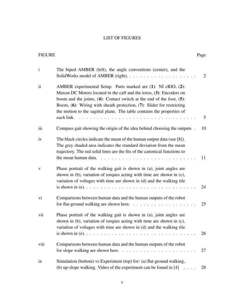
i The biped AMBER (left), the angle conventions (center), and theSolidWorks model of AMBER (right). . . . . . . . . . . . . . . . . . . . 2

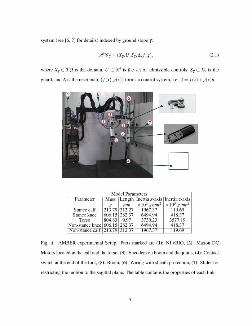
ii AMBER experimental Setup. Parts marked are (1): NI cRIO, (2):Maxon DC Motors located in the calf and the torso, (3): Encoders onboom and the joints, (4): Contact switch at the end of the foot, (5):Boom, (6): Wiring with sheath protection, (7): Slider for restrictingthe motion to the sagittal plane. The table contains the properties ofeach link. . . . . . . . . . . . . . . . . . . . . . . . . . . . . . . . . . 5

iii Compass gait showing the origin of the idea behind choosing the outputs . 10

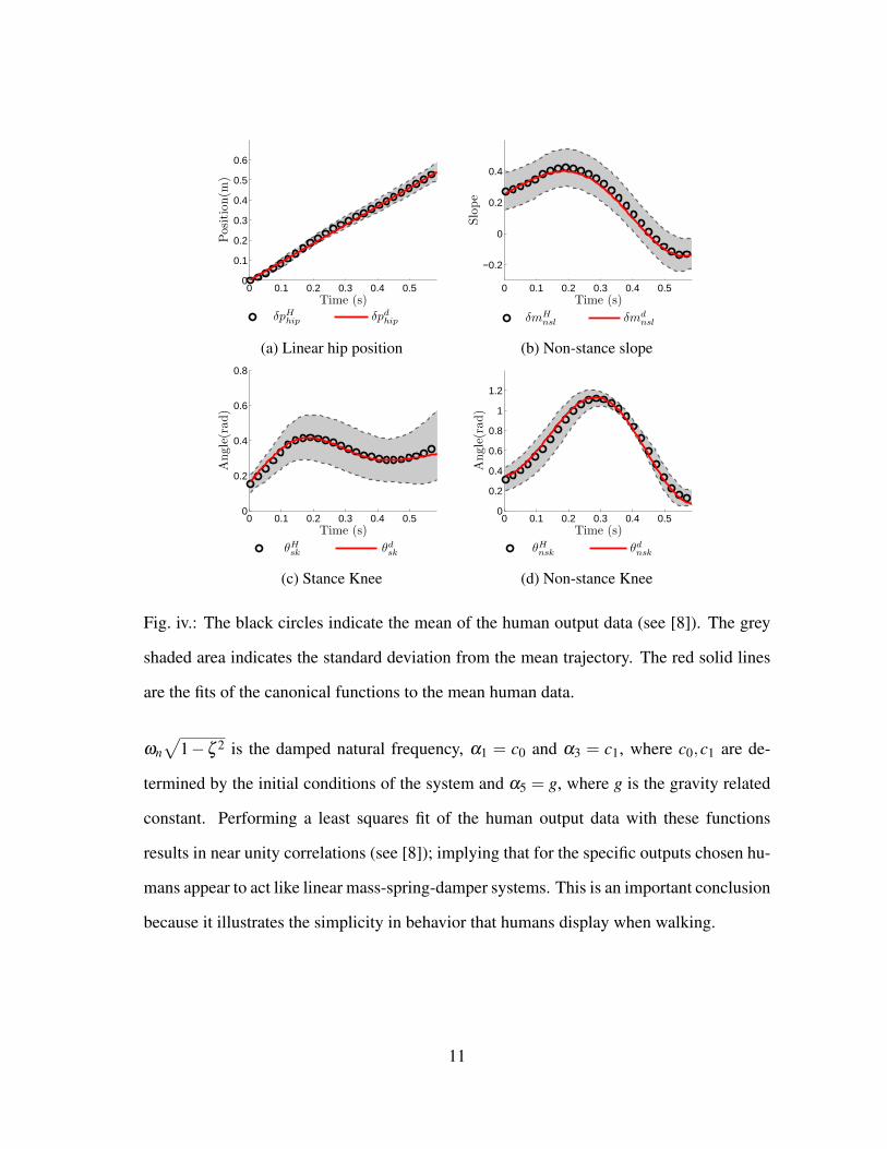
iv The black circles indicate the mean of the human output data (see [8]).The grey shaded area indicates the standard deviation from the meantrajectory. The red solid lines are the fits of the canonical functions tothe mean human data. . . . . . . . . . . . . . . . . . . . . . . . . . . . 11

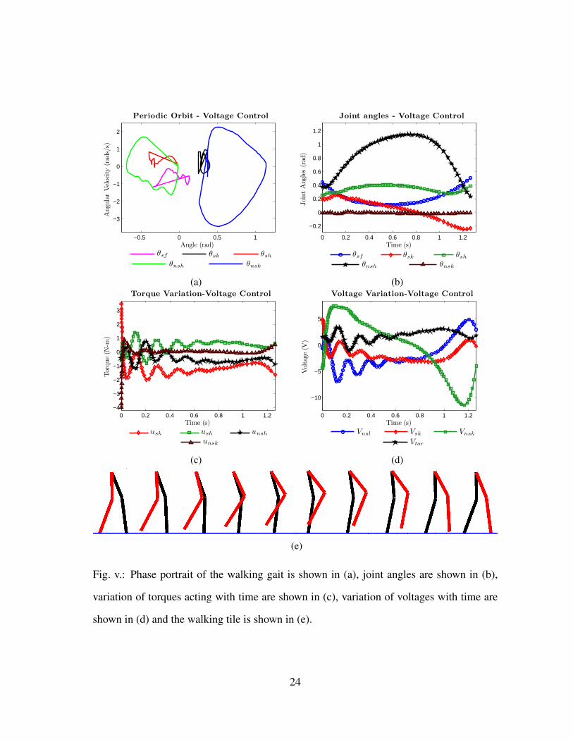
v Phase portrait of the walking gait is shown in (a), joint angles areshown in (b), variation of torques acting with time are shown in (c),variation of voltages with time are shown in (d) and the walking tileis shown in (e). . . . . . . . . . . . . . . . . . . . . . . . . . . . . . . . 24

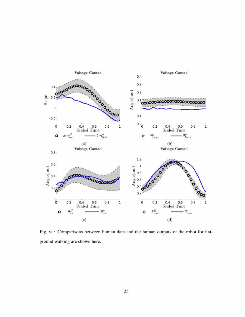
vi Comparisons between human data and the human outputs of the robotfor flat-ground walking are shown here. . . . . . . . . . . . . . . . . . . 25

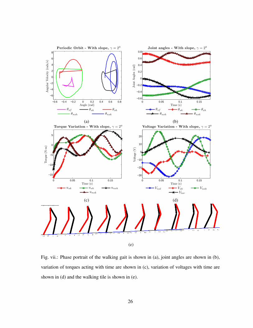
vii Phase portrait of the walking gait is shown in (a), joint angles areshown in (b), variation of torques acting with time are shown in (c),variation of voltages with time are shown in (d) and the walking tileis shown in (e). . . . . . . . . . . . . . . . . . . . . . . . . . . . . . . . 26

viii Comparisons between human data and the human outputs of the robotfor slope walking are shown here. . . . . . . . . . . . . . . . . . . . . . 27

ix Simulation (bottom) vs Experiment (top) for: (a) flat-ground walking,(b) up-slope walking. Video of the experiment can be found in [4] . . . . 28

v

x Experimental (blue) vs. simulated (red) angles over 10 steps for flat-ground walking. . . . . . . . . . . . . . . . . . . . . . . . . . . . . . . 29

xi Experimental (blue) vs. simulated (red) angles over 10 steps for up-slope walking. . . . . . . . . . . . . . . . . . . . . . . . . . . . . . . . 30

xii Graphical representation of IMT is shown here. . . . . . . . . . . . . . . 36

xiii Phase portraits and outputs of AMBER walking over a randomly gen-erated terrain (left) and a sinusoidal terrain (right). . . . . . . . . . . . . . 37

xiv AMBER with the treadmill, and the linear actuator (back) used to varythe slope of the terrain. . . . . . . . . . . . . . . . . . . . . . . . . . . . 38

xv Tiles showing AMBER taking one step on the rough terrain. It can beobserved that the configuration of the robot at the end of the step isdifferent from the beginning of the step. . . . . . . . . . . . . . . . . . . 40

xvi Comparison of outputs of the robot with the desired outputs. Sincethe stance knee takes the weight of the robot, it does not match withthe desired output well. . . . . . . . . . . . . . . . . . . . . . . . . . . 40

xvii Desired output functions from the intermediate transition matrix α int

computed at all the steps (red waveforms) and compared with the hu-man data (shown in blue). . . . . . . . . . . . . . . . . . . . . . . . . . 41

vi

CHAPTER I

INTRODUCTION

One of the key characteristics that distincts humans from other animals is the stance pos-

ture. Human evolution has made the two legs as the only tools for locomotion in humans. In

other words, human evolution has made and continuously improved bipedal (two legged)

walking to an extent that it can exhibit amazingly robust behaviors over a wide variety

of terrains in the environment. This is one of the factors why emulating human walking

has been a continued objective for a majority of bipedal walking researchers. Humans are

believed to use their spinal cords to generate simple patterns, which excite the muscles

in a periodic manner producing a rhythm, resulting in walking (see [16, 21]). This allows

people to walk without needing to think about it. This was one of the motivating factors be-

hind conceiving the idea of human-inspired walking in [6], and this thesis essentially shows

how to achieve human-like walking with AMBER on three kinds of terrains–flat-ground,

up-slope and rough terrain.

Some of the first fundamental work in bipedal robotic walking was by Marc Raibert,

with the idea of achieving locomotion through the use of inverted pendulum models to

create single-legged hoppers [24], and Tad Mcgeer who introduced the concept of passive

walking [19] (which has also been realized in robots with efficient actuation [12]). Passive

walking lead to the notion of controlled symmetries [27] which allows for low energy

walking, and the Spring Loaded Inverted Pendulum (SLIP) models [15, 23] for running

robots. Walking has also been looked at as a metastable process and extended to stochastic

rough terrain walking [11]. In addition to these “minimalist” approaches, several methods

have been proposed to directly bridge the gap between biomechanics and control theory

by looking at human walking data to build models for bipedal robotic walking (see [13,

1

z

x

èsf

èsh

ènsh

èsk

ènsk

Fig. i.: The biped AMBER (left), the angle conventions (center), and the SolidWorks model

of AMBER (right).

28] to name a few). Finally, combining many of the above approaches, significant strides

have been made in underactuated bipedal walking (no feet) by using the idea of virtual

constraints and Hybrid Zero Dynamics (HZD) [29, 18], which resulted in amazingly robust

walking even on rough terrain. HZD has indeed represented bipedal walking in a very

elegant fashion, but implementing a HZD controller on a biped involves the determination

of the parameters of the robot through identification experiments [22] which are not only

very exhaustive and time consuming but also not scalable to changes in hardware or robot

structure.

Similar to [29], the technique that we adopt also considers trajectory tracking of a

special set of functions called canonical walking functions (CWF) (see [6, 9, 26, 8, 7]. The

CWF are obtained from running an optimization problem such that the resulting walking

obtained is as close to human data as possible. One of the essential components of this

thesis that stands out is that there are no low level control loops running in the robot. The

walking algorithm is solely based on the control voltage that is provided by the controller

purely as a function of the CWF. This is as close as we get toward emulating the central

2

pattern generators in humans and claim that the simple excitation of the motor actuators by

these CWF based on the configuration of the robot results in walking.

The main contribution of this thesis is to design experimentally realizable control laws

to achieve walking with AMBER (Fig. i) for three different kinds of motion primitives:

flat-ground, up-slope and rough terrain. We begin by introducing a formal model of AM-

BER, including both its mechanical and electrical components in Chapter II; the fidelity of

this model is essential for predicting experimental behavior through simulation. Using the

human-inspired control suggested in Chapter III, steady state walking is achieved on a con-

stant slope, γ , in simulation. This is tried in AMBER by using proportional voltage control,

which justifies the control methodology suggested. Chapter IV explains this experimental

implementation. Specifically, we do it by using the parameters of outputs obtained from the

formal optimization problem that provably results in stable robotic walking, and define a

simple voltage-based proportional (P) feedback control law on the human-inspired outputs

(similar ideas have been explored for robotic manipulators [10, 17]). Since the actuators of

AMBER are powered by DC motors, this naturally lends itself to simple implementation on

the physical robot. The end result is that the voltage applied to the motors is directly pro-

portional to the error between the desired and actual outputs of the robot, as represented by

the canonical walking functions. This stable walking on a plane of slope γ is then extended

to a terrain of varying slopes in Chapter V. In other words, formal controllers are developed

for achieving provably stable walking on a rough terrain. We start with flat ground, and use

the reference CWF for flat ground (it is obtained from [30]). The walking is achieved in

such a way that it respects Hybrid Zero Dynamics. Hybrid Zero Dynamics (HZD) is the

equivalent of zero dynamics in hybrid systems. In other words, this means that the actuated

outputs of the robot are tracking the desired functions even through impacts. Then, we

allow small perturbations in the terrain, i.e., allow small changes in slopes (γ) and generate

new CWF in such a way that it brings it back to normal flat ground walking mode.

3

CHAPTER II

BIPEDAL ROBOTIC MODEL

This chapter explains the mechanical and electrical model of AMBER. The importance of

making an accurate model lies in the application of the linearizing controller on the robot

to get provable walking results.

II.1. Biped Description

AMBER is a 2D bipedal robot with five links (two calves, two thighs and a torso, see

Fig. ii). AMBER is 61 cm tall with a total mass of 3.3 kg (see Fig. ii). It is made from

aluminum with carbon fiber calves, powered by 4 DC motors and controlled through Lab-

VIEW software by National Instruments. The robot has point feet, and is thus underactu-

ated at the ankle. In addition, since this robot is built for only 2D walking, it is supported in

the lateral plane via a boom; this boom does not provide support to the robot in the sagittal

plane. This means that the torso, through which the boom supports the robot, can freely

rotate around the boom. The boom is fixed rigidly to a sliding mechanism (see Fig. ii),

which allows the boom and consequently the biped, to move its hip front, back, up and

down with minimum friction. The sliding mechanism is rested on a pair of parallel rails.

In addition, the whole robot ambulates on a treadmill. In this manner, we can also achieve

slope walking by just changing the slope (γ) of the treadmill.

Define the configuration space Q with θ = (θs f ,θsk,θsh,θnsh,θnsk)T ∈ Q containing

the relative angles between links as shown in Fig. i. When the foot hits the ground, the

stance and non-stance legs are swapped. Formally, we represent the robot as a hybrid

4

system (see [6, 7] for details) indexed by ground slope γ:

H C γ = (Xγ ,U,Sγ ,∆, f ,g), (2.1)

where Xγ ⊂ T Q is the domain, U ⊂ R4 is the set of admissible controls, Sγ ⊂ Xγ is the

guard, and ∆ is the reset map. ( f (x),g(x)) forms a control system, i.e., x = f (x)+g(x)u.

15

3

3

3

2

4

2

7

6

Model ParametersParameter Mass Length Inertia x-axis Inertia z-axis

g mm ×103 g mm2 ×103 g mm2

Stance calf 213.79 312.27 1967.37 119.69Stance knee 606.15 282.37 6494.94 418.37

Torso 804.83 9.97 3730.23 3577.19Non-stance knee 606.15 282.37 6494.94 418.37Non-stance calf 213.79 312.37 1967.37 119.69

Fig. ii.: AMBER experimental Setup. Parts marked are (1): NI cRIO, (2): Maxon DC

Motors located in the calf and the torso, (3): Encoders on boom and the joints, (4): Contact

switch at the end of the foot, (5): Boom, (6): Wiring with sheath protection, (7): Slider for

restricting the motion to the sagittal plane. The table contains the properties of each link.

5

Continuous Dynamics. Calculating the inertial properties of each link of the robot (Fig. i)

yields the Lagrangian,

L(θ , θ) =12

θT D(θ)θ −V (θ). (2.2)

Explicitly, this is done symbolically through the method of exponential twists (see [20]).

The inertias of the motors and boom are also included. Let Ir, Ig, Im be the rotational

inertias of the rotor, gearbox, and motor, respectively. Then, Im = Irr2 + Ig, where r = 157

is the gear ratio. Because r is large, Ig can be ignored. Each joint is connected to a motor

through a metal chain. Therefore, the axis of rotation of the rotor has an offset w.r.t. that

of the link. Using the parallel axis theorem: Ip = Im +mmd2m, where Ip is the motor inertia

shifted to the joint axis, mm is the mass of the rotating motor parts, and dm is the distance

between axes. Again, since mm = 0.011 kg, Ip ≈ Im.

The boom is rigidly bolted to the sliders and thus does not rotate w.r.t. the world frame.

Therefore, only the translational inertia of the boom is considered. Let mx (resp. mz) denote

the mass of the parts in the boom-slider moving forward and backward (resp. upward and

downward). Then, the resulting mass matrix is Mboom ∈ R6×6 where (Mboom)1,1 = mx and

(Mboom)3,3 = mz with all other entries equal to zero. The combined inertia matrix, Dcom,

used in the Lagrangian is

Dcom(θ) = D(θ)+diag(0, Im,sk, Im,sh, Im,nsh, Im,nsk)

+J(θ)T MboomJ(θ), (2.3)

where Im,sk, Im,sh, Im,nsh, Im,nsk represent the motor inertias of the links and J(θ) is the body

Jacobian of the torso center of mass. The Euler-Lagrange equation yields a dynamic model:

Dcom(θ)θ +H(θ , θ) = B(θ)u, (2.4)

6

where the control, u, is a vector of torque inputs. Since AMBER has DC motors, we need

to derive equations with voltage inputs. Since the motor inductances are small, we can

realize the electromechanical system:

Vin = Raia +Kωω, (2.5)

where Vin is the vector of voltage inputs to the motors, ia is the vector of currents through

the motors, and Ra is the resistance matrix. Since the motors are individually controlled,

Ra is a diagonal matrix. Kω is the motor constant matrix and ω is a vector of angular

velocities of the motors. Representing (2.5) in terms of currents, the applied torque is

u = KϕR−1a (Vin−Kωω), with Kϕ the torque constant matrix. Thus, the Euler-Lagrange

equation takes the form Dcom(θ)θ +H(θ , θ) = B(θ)KϕR−1a (Vin−Kωω).

Converting this model to first order ODEs yields the affine control system ( fv,gv) with

inputs Vin:

fv(θ , θ) =

θ

−D−1com(θ)(H(θ , θ)+B(θ)KϕR−1

a Kωω)

,gv(θ) =

0

D−1com(θ)B(θ)KϕR−1

a

. (2.6)

Discrete Dynamics. The domain, Xγ , describes the allowable state space restricted by the

guard, hγ . For AMBER, the non-stance foot must be above a slope of γ , i.e., hγ ≥ 0:

Xγ ={(θ , θ) ∈ T Q : hγ(θ)≥ 0

},

The guard is just the boundary of the domain with the additional assumption that hγ is

decreasing:

Sγ ={(θ , θ) ∈ T Q : hγ(θ) = 0 and dhγ(θ)θ < 0

},

7

with dhγ(θ) the Jacobian of hγ at θ . When the non-stance foot impacts the ground, the

angular velocities change. Hence we define a reset map, ∆ : Sγ → Xγ which maps the

pre-impact state to the post-impact state; see [6] for details.

8

CHAPTER III

HUMAN-INSPIRED CONTROL

This section reviews human-inspired control which is the approach we use to achieve walk-

ing both in simulation and experiment on a given known terrain. For simplicity, we will

describe the control law for flat ground walking which are described in detail in [7] (also

see [6, 8] for related results in the case of full actuation and [31] for results on other kinds

of terrains). The idea will be to extended from flat-ground walking to up-slope walking and

then finally to walking on rough terrain.

III.1. Human-Inspired Functions

By considering human walking data (as described in [6]), we discover that certain outputs

(or virtual constraints), computed from the human joint data, display simple behavior; this

core observation will be central to the design of human-inspired controllers. With the

goal of picking outputs that elucidate the underlying structure of walking through a low-

dimensional representation, or “virtual model,” we pick outputs that represent the human

(and bipedal robot) as a compass-gait biped [12, 19] and the SLIP model [15]. In particular,

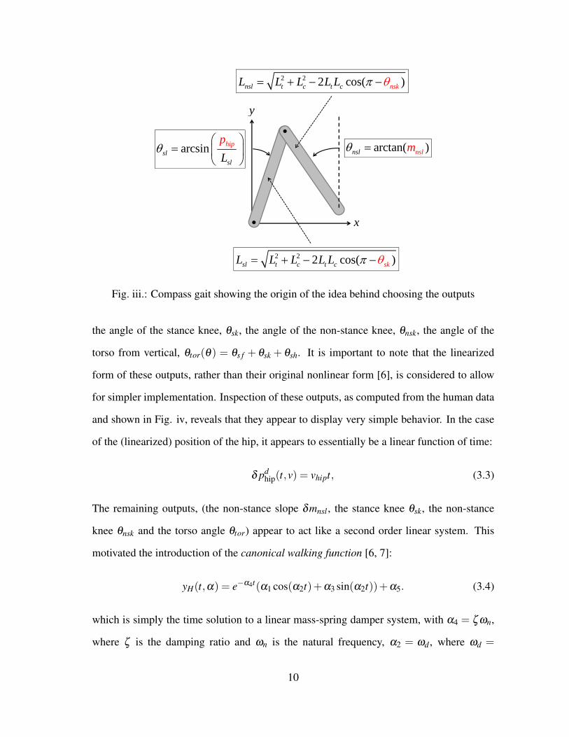
the following collection of outputs yields such a representation (as illustrated in Fig. iii):

the linearization of the x-position of the hip, phip, given by:

δ phip(θ) = Lc(−θs f )+Lt(−θs f −θsk), (3.1)

the linearization of the slope of the non-stance leg mnsl , (the tangent of the angle between

the z-axis and the line on the non-stance leg connecting the ankle and hip), given by:

δmnsl(θ) =−θs f −θsk−θsh +θnsh +Lc

Lc +Ltθnsk, (3.2)

9

arcsin hsl

sl

ippL

arctan( )sl lns nm

x

y

2 2 2 cos( )sl t c st c kL L L L L

2 2 2 cos( )nsl t c skt ncL L L L L

Fig. iii.: Compass gait showing the origin of the idea behind choosing the outputs

the angle of the stance knee, θsk, the angle of the non-stance knee, θnsk, the angle of the

torso from vertical, θtor(θ) = θs f + θsk + θsh. It is important to note that the linearized

form of these outputs, rather than their original nonlinear form [6], is considered to allow

for simpler implementation. Inspection of these outputs, as computed from the human data

and shown in Fig. iv, reveals that they appear to display very simple behavior. In the case

of the (linearized) position of the hip, it appears to essentially be a linear function of time:

δ pdhip(t,v) = vhipt, (3.3)

The remaining outputs, (the non-stance slope δmnsl , the stance knee θsk, the non-stance

knee θnsk and the torso angle θtor) appear to act like a second order linear system. This

motivated the introduction of the canonical walking function [6, 7]:

yH(t,α) = e−α4t(α1 cos(α2t)+α3 sin(α2t))+α5. (3.4)

which is simply the time solution to a linear mass-spring damper system, with α4 = ζ ωn,

where ζ is the damping ratio and ωn is the natural frequency, α2 = ωd , where ωd =

10

0 0.1 0.2 0.3 0.4 0.50

0.1

0.2

0.3

0.4

0.5

0.6

Time (s)

Posi

tion(m

)

δpHhip δpd

hip

(a) Linear hip position

0 0.1 0.2 0.3 0.4 0.5

−0.2

0

0.2

0.4

Time (s)

Slo

pe

δmHnsl δmd

nsl

(b) Non-stance slope

0 0.1 0.2 0.3 0.4 0.50

0.2

0.4

0.6

0.8

Time (s)

Angle

(rad)

θHsk θd

sk

(c) Stance Knee

0 0.1 0.2 0.3 0.4 0.50

0.2

0.4

0.6

0.8

1

1.2

Time (s)

Angle

(rad)

θHnsk θd

nsk

(d) Non-stance Knee

Fig. iv.: The black circles indicate the mean of the human output data (see [8]). The grey

shaded area indicates the standard deviation from the mean trajectory. The red solid lines

are the fits of the canonical functions to the mean human data.

ωn√

1−ζ 2 is the damped natural frequency, α1 = c0 and α3 = c1, where c0,c1 are de-

termined by the initial conditions of the system and α5 = g, where g is the gravity related

constant. Performing a least squares fit of the human output data with these functions

results in near unity correlations (see [8]); implying that for the specific outputs chosen hu-

mans appear to act like linear mass-spring-damper systems. This is an important conclusion

because it illustrates the simplicity in behavior that humans display when walking.

11

III.2. Human-Inspired Controller

Having defined the outputs, we can construct a controller that drives four of the outputs of

the robot (one output, which is the hip position, is omitted since AMBER is an underactu-

ated robot and it is not possible to drive five outputs with four actuators) to the outputs of

the human, as represented by the CWF: ya(θ(t))→ yd(t,α), with:

yd(t,α) = [yH(t,αnsl),yH(t,αsk),yH(t,αnsk),yH(t,αtor)]T ,

ya(θ) = [δmnsl(θ),θsk,θnsk,θtor(θ)]T , (3.5)

where yH(t,αi), i∈{nsl,sk,nsk, tor} is the CWF (5.4) but with parameters αi specific to the

output being considered. Grouping these parameters with the velocity of the hip, vhip, that

appears in (3.3), results in the vector of parameters α = (vhip,αnsl,αsk,αnsk,αtor) ∈ R21.

We can remove the dependence of time in yd(t,α) based upon the fact that the (lin-

earized) position of the hip is accurately described by a linear function of time:

τ(θ) = (δ pRhip(θ)−δ pR

hip(θ+))/vhip, (3.6)

where δ pRhip(θ

+) is the linearized position of the hip at the beginning of a step. θ+ is the

configuration where the height of the non-stance foot is zero, i.e., hγ(θ+) = 0. Using (3.6),

we define the following human-inspired output:

yα(θ) = ya(θ)− yd(τ(θ),α). (3.7)

Control Law Construction. The outputs were chosen so that the decoupling matrix,

A(θ , θ) = LgL f yα(θ , θ) with L the Lie derivative, is nonsingular. Therefore, the outputs

12

have (vector) relative degree 2 and we can define the following torque controller:

u(α,ε)(θ , θ) = (3.8)

−A−1(θ , θ)(L2

f yα(θ , θ)+2εL f yα(θ , θ)+ ε2yα(θ)

).

In other words, we can apply feedback linearization to obtain the linear system on the

human-inspired output: yα =−2ε yα−ε2yα . This system is exponentially stable, implying

that for ε > 0 the control law u(α,ε) drives yα → 0 as t→ ∞ (see [25]).

III.3. Human-Inspired Hybrid Zero Dynamics (HZD)

The goal of the human-inspired controller (3.8) was to drive the outputs of the robot to the

outputs of the human: ya→ yd . And as t → ∞, ya→ yd . But, due to the occurrence of the

impact with every step, this may not be true all the time. Therefore, the goal of this section

is to find the CWF for which this is satisfied and represent the zero dynamics surface.

Problem Statement. Since the robot is underactuated, some of the variables in the state

will not be controllable; and since AMBER is a mechanical system, the number of variables

is 2. This leads to the notion of using the zero dynamics surface which has a dimension of

2. The control law is applied in such a way that the controllable outputs are forced to 0 as

t → ∞. As long as these outputs are exponentially stable, we can realize a surface which

represents bipedal robotic walking. Therefore, with the human-inspired controller applied,

we say that the controller renders the zero dynamics surface:

Zα = {(θ , θ) ∈ T Q : yα(θ) = 0, L f yα(θ , θ) = 0} (3.9)

exponentially stable; moreover, this surface is invariant for the continuous dynamics. Note

that here 0 ∈ R4 is a vector of zeros and we make the dependence of Zα on the set of

parameters explicit. It is at this point that continuous systems and hybrid systems diverge:

13

while this surface is invariant for the continuous dynamics, it is not necessarily invariant

for the hybrid dynamics. In particular, the discrete impacts in the system cause the state to

be “thrown” off of the zero dynamics surface. Therefore, a hybrid system has Hybrid Zero

Dynamics if the zero dynamics are invariant through impact: ∆(S∩Zα)⊂ Zα .

The goal of human-inspired HZD is to find parameters α∗ that solve the following

constrained optimization problem:

α∗ = argmin

α∈R21CostHD(α) (3.10)

s.t ∆(S∩Zα)⊂ Zα (HZD)

with CostHD the least squares fit of the CWF with the human data. This determines the

parameters of the CWF that gave the best fit of the human walking functions to the human

output data, but subject to constraints that ensure HZD. To get provable and physically

realizable walking, other constraints are imposed like non-stance foot height clearance,

torque and velocity constraints (see [30]). The optimization also produces a fixed point

(θ(ϑ(α), θ(ϑ(α)) of the periodic gait which can be used to compute the transitions on

rough terrain. Space constraints limit the explanation of the guard configuration of the

robot, ϑ(α), and it can be found in [7].

Zero Dynamics. With the control law ensuring HZD, we can explicitly construct the zero

dynamics surface. In particular, we utilize the constructions in [29], reframed in the context

of canonical human walking functions.

ξ1 = δ pRhip(θ) =: cθ (3.11)

ξ2 = D(θ)1,1θ =: γ0(θ)θ

where c ∈ R5×1 is obtained from (3.1), and D(θ)1,1 is the first entry of the inertia matrix

in (2.2). Moreover, since ξ1 is just the linearized position of the hip, which was used to

14

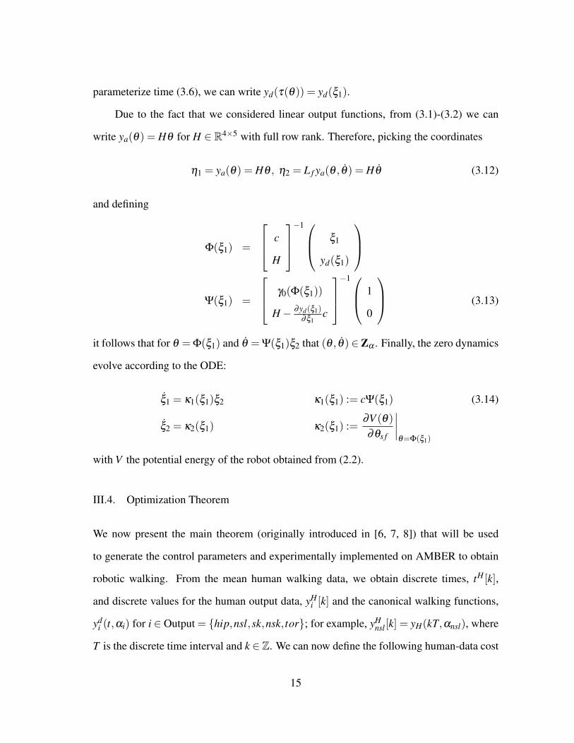
parameterize time (3.6), we can write yd(τ(θ)) = yd(ξ1).

Due to the fact that we considered linear output functions, from (3.1)-(3.2) we can

write ya(θ) = Hθ for H ∈ R4×5 with full row rank. Therefore, picking the coordinates

η1 = ya(θ) = Hθ , η2 = L f ya(θ , θ) = Hθ (3.12)

and defining

Φ(ξ1) =

c

H

−1 ξ1

yd(ξ1)

Ψ(ξ1) =

γ0(Φ(ξ1))

H− ∂yd(ξ1)∂ξ1

c

−1 1

0

(3.13)

it follows that for θ = Φ(ξ1) and θ = Ψ(ξ1)ξ2 that (θ , θ)∈Zα . Finally, the zero dynamics

evolve according to the ODE:

ξ1 = κ1(ξ1)ξ2 κ1(ξ1) := cΨ(ξ1) (3.14)

ξ2 = κ2(ξ1) κ2(ξ1) :=∂V (θ)

∂θs f

∣∣∣∣θ=Φ(ξ1)

with V the potential energy of the robot obtained from (2.2).

III.4. Optimization Theorem

We now present the main theorem (originally introduced in [6, 7, 8]) that will be used

to generate the control parameters and experimentally implemented on AMBER to obtain

robotic walking. From the mean human walking data, we obtain discrete times, tH [k],

and discrete values for the human output data, yHi [k] and the canonical walking functions,

ydi (t,αi) for i ∈ Output = {hip,nsl,sk,nsk, tor}; for example, yH

nsl[k] = yH(kT,αnsl), where

T is the discrete time interval and k ∈ Z. We can now define the following human-data cost

15

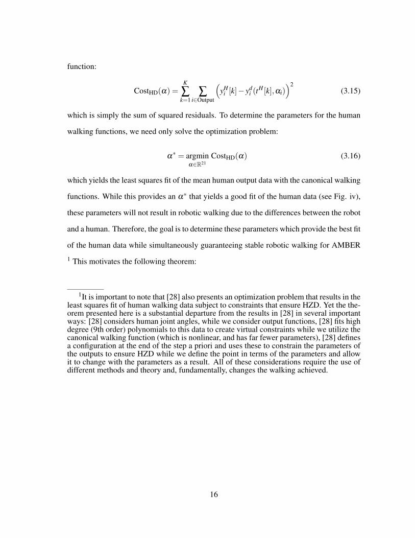
function:

CostHD(α) =K

∑k=1

∑i∈Output

(yH

i [k]− ydi (t

H [k],αi))2

(3.15)

which is simply the sum of squared residuals. To determine the parameters for the human

walking functions, we need only solve the optimization problem:

α∗ = argmin

α∈R21CostHD(α) (3.16)

which yields the least squares fit of the mean human output data with the canonical walking

functions. While this provides an α∗ that yields a good fit of the human data (see Fig. iv),

these parameters will not result in robotic walking due to the differences between the robot

and a human. Therefore, the goal is to determine these parameters which provide the best fit

of the human data while simultaneously guaranteeing stable robotic walking for AMBER

1 This motivates the following theorem:

1It is important to note that [28] also presents an optimization problem that results in theleast squares fit of human walking data subject to constraints that ensure HZD. Yet the the-orem presented here is a substantial departure from the results in [28] in several importantways: [28] considers human joint angles, while we consider output functions, [28] fits highdegree (9th order) polynomials to this data to create virtual constraints while we utilize thecanonical walking function (which is nonlinear, and has far fewer parameters), [28] definesa configuration at the end of the step a priori and uses these to constrain the parameters ofthe outputs to ensure HZD while we define the point in terms of the parameters and allowit to change with the parameters as a result. All of these considerations require the use ofdifferent methods and theory and, fundamentally, changes the walking achieved.

16

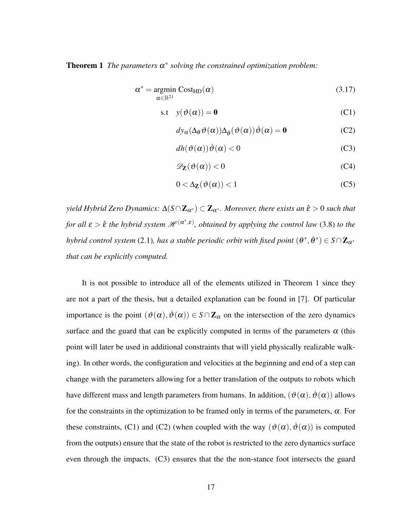
Theorem 1 The parameters α∗ solving the constrained optimization problem:

α∗ = argmin

α∈R21CostHD(α) (3.17)

s.t y(ϑ(α)) = 0 (C1)

dyα(∆θ ϑ(α))∆θ(ϑ(α))ϑ(α) = 0 (C2)

dh(ϑ(α))ϑ(α)< 0 (C3)

DZ(ϑ(α))< 0 (C4)

0 < ∆Z(ϑ(α))< 1 (C5)

yield Hybrid Zero Dynamics: ∆(S∩Zα∗)⊂ Zα∗ . Moreover, there exists an ε > 0 such that

for all ε > ε the hybrid system H (α∗,ε), obtained by applying the control law (3.8) to the

hybrid control system (2.1), has a stable periodic orbit with fixed point (θ ∗, θ ∗) ∈ S∩Zα∗

that can be explicitly computed.

It is not possible to introduce all of the elements utilized in Theorem 1 since they

are not a part of the thesis, but a detailed explanation can be found in [7]. Of particular

importance is the point (ϑ(α), ϑ(α)) ∈ S∩Zα on the intersection of the zero dynamics

surface and the guard that can be explicitly computed in terms of the parameters α (this

point will later be used in additional constraints that will yield physically realizable walk-

ing). In other words, the configuration and velocities at the beginning and end of a step can

change with the parameters allowing for a better translation of the outputs to robots which

have different mass and length parameters from humans. In addition, (ϑ(α), ϑ(α)) allows

for the constraints in the optimization to be framed only in terms of the parameters, α . For

these constraints, (C1) and (C2) (when coupled with the way (ϑ(α), ϑ(α)) is computed

from the outputs) ensure that the state of the robot is restricted to the zero dynamics surface

even through the impacts. (C3) ensures that the the non-stance foot intersects the guard

17

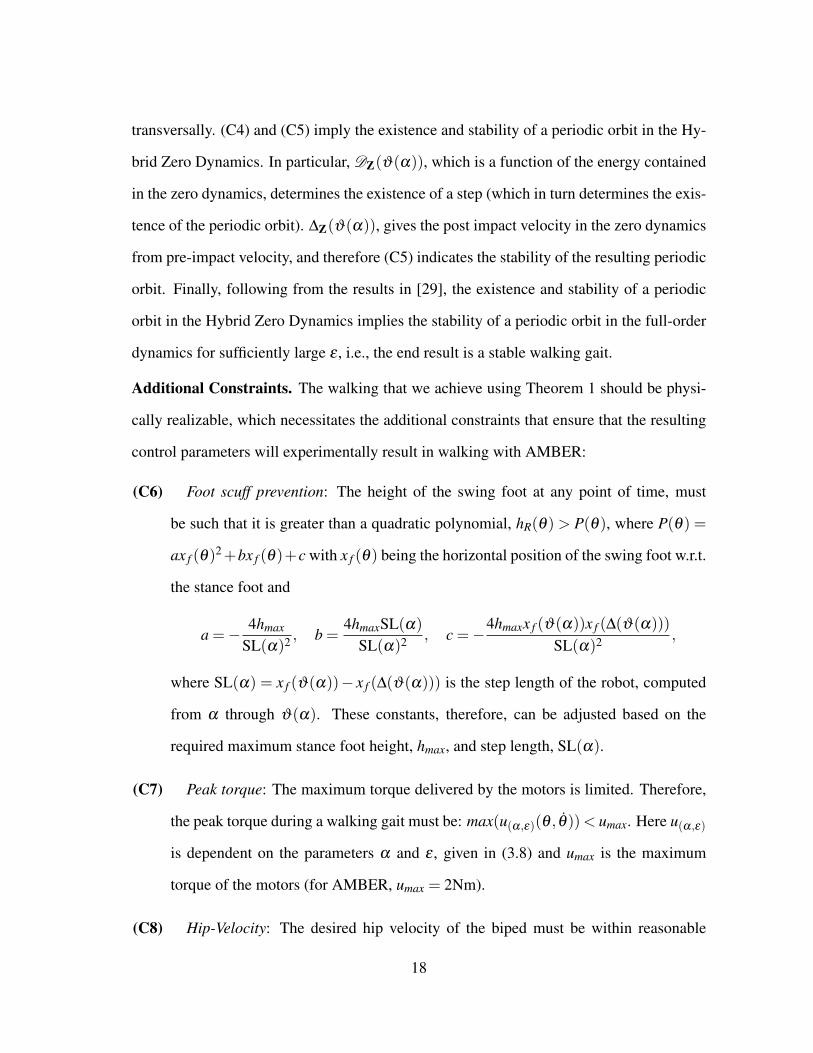
transversally. (C4) and (C5) imply the existence and stability of a periodic orbit in the Hy-

brid Zero Dynamics. In particular, DZ(ϑ(α)), which is a function of the energy contained

in the zero dynamics, determines the existence of a step (which in turn determines the exis-

tence of the periodic orbit). ∆Z(ϑ(α)), gives the post impact velocity in the zero dynamics

from pre-impact velocity, and therefore (C5) indicates the stability of the resulting periodic

orbit. Finally, following from the results in [29], the existence and stability of a periodic

orbit in the Hybrid Zero Dynamics implies the stability of a periodic orbit in the full-order

dynamics for sufficiently large ε , i.e., the end result is a stable walking gait.

Additional Constraints. The walking that we achieve using Theorem 1 should be physi-

cally realizable, which necessitates the additional constraints that ensure that the resulting

control parameters will experimentally result in walking with AMBER:

(C6) Foot scuff prevention: The height of the swing foot at any point of time, must

be such that it is greater than a quadratic polynomial, hR(θ) > P(θ), where P(θ) =

ax f (θ)2+bx f (θ)+c with x f (θ) being the horizontal position of the swing foot w.r.t.

the stance foot and

a =− 4hmax

SL(α)2 , b =4hmaxSL(α)

SL(α)2 , c =−4hmaxx f (ϑ(α))x f (∆(ϑ(α)))

SL(α)2 ,

where SL(α) = x f (ϑ(α))− x f (∆(ϑ(α))) is the step length of the robot, computed

from α through ϑ(α). These constants, therefore, can be adjusted based on the

required maximum stance foot height, hmax, and step length, SL(α).

(C7) Peak torque: The maximum torque delivered by the motors is limited. Therefore,

the peak torque during a walking gait must be: max(u(α,ε)(θ , θ))< umax. Here u(α,ε)

is dependent on the parameters α and ε , given in (3.8) and umax is the maximum

torque of the motors (for AMBER, umax = 2Nm).

(C8) Hip-Velocity: The desired hip velocity of the biped must be within reasonable

18

limits. Therefore, we introduce the constraint: vmin < vhip < vmax. For AMBER,

vmin = 0.1m/s, vmax = 0.6m/s.

(C9) Angular velocities of joints: The maximum angular velocities with which the joints

can turn are limited by the maximum angular velocities of the motors. The motors

used in AMBER have a maximum angular velocity of 6.5rad/s.

19

CHAPTER IV

FLAT-GROUND AND UP-SLOPE WALKING IN AMBER

The control law proposed in the previous section requires us to linearize the dynamics of

AMBER through model inversion, which requires exact values of masses, inertias and di-

mensions of the robot. This is not only complex to implement but realizing the control

law (3.8) on AMBER could potentially consume both time and resources, and achieving

walking may still not be guaranteed due to a potentially inexact model. We, therefore, take

the different approach by arguing that due to the “correct” choice of output functions—and

specifically the human-inspired outputs—it is possible to obtain walking through simple

controllers that are easy to implement and inherently more robust. Specifically, we present

a proportional voltage controller on the human-inspired outputs, and demonstrate through

simulation that robotic walking is obtained on AMBER. The simplicity of this controller

implies that it can be efficiently implemented in software, and the details of this implemen-

tation are given. Finally, experimental results are presented showing that bipedal robotic

walking is obtained with AMBER that is both efficient and robust.

IV.1. Human-Inspired Voltage Control

Even if walking is obtained formally through input/output linearization, i.e., model inver-

sion, the controllers are often implemented through PD control on the torque (see, for ex-

ample, [22]). Since AMBER is not equipped with torque sensors, we sought an alternative

method for feedback control implementation. Because AMBER is powered by DC motors,

the natural input to consider is voltage, Vin, which indirectly affects the torques acting on

the joints.

Let Vsk be the voltage input to the stance knee motor, Vnsk be the voltage input to the

20

non-stance knee motor, Vnsl be the voltage input to the non-stance hip motor and finally Vtor

be the voltage input to the stance hip of the motor. Then the following proportional control

law is defined:

Vnsl(t,θ) = −Kp,nsl(θsk−θdsk(t,αsk)), (4.1)

Vsk(t,θ) = −Kp,sk(θnsk−θdnsk(t,αnsk)),

Vnsk(t,θ) = −Kp,nsk(δmRnsl(θ)−md

nsl(t,αnsl)),

Vtor(t,θ) = −Kp,tor(θRtor(θ)−θ

dtor(t,αtor)),

where Kp,nsl,Kp,sk,Kp,nsk,Kp,tor are the diagonal entries of the matrix Kp. The non-diagonal

entries are 0. If time is parameterised w.r.t hip position, then the variable t in (4.1) will be

replaced with τ(θ) from (3.6). Therefore, (4.1) can be written in this form:

Vin =

Vnsl(τ(θ),θ)

Vsk(τ(θ),θ)

Vnsk(τ(θ),θ)

Vtor(τ(θ),θ)

= −Kpy(θ), (4.2)

It can be seen that the control law (proportional control) solely depends on the gen-

eralized coordinates of robot (angles), θ , and not on the angular velocities. This marks

a drastic change from the traditional ways of computing control. Evidently, and impor-

tantly, this avoids computation of angular velocities of the joints, which would have been

computationally expensive and inaccurate.

It is important to note that the P voltage control law (4.2) is equivalent to a PD torque

controller, where the derivative (D) constant is specified by the properties of the motor.

Given the voltage input, the torque vector acting on the links is obtained by:

u(θ) =−KϕR−1a Kpy(θ)−KϕR−1

a Kωω. (4.3)

21

We can see that P-control with voltage as the input actually leads to P-control with torque

as an input with an added velocity term. Hence, the control being applied is not markedly

different from the conventional torque control methods adopted in literature (see [14]).

IV.2. Simulation and Experimental Results

By applying the new voltage control law on each of the motors we get the following results.

IV.2.1. Flat-ground walking

For implementing flat-ground walking, we numerically solve the optimization algorithm

in Theorem 1 subject to the additional constraints (C6)-(C9) to obtain the optimized pa-

rameter α∗ corresponding to zero slope γ = 0. By applying the control law given in (4.2),

parameterized by α∗, to the control system ( fv(x),gv(x)) yields walking on flat ground.

Periodic orbit of the walking gait obtained is shown in Fig. v(a), tiles of the walking ob-

tained in simulation can be seen in Fig. v(e). In Fig. vi(a)-(d) the outputs of the robot are

compared with the mean human data. Again, we can deduce that the output functions are

amazingly close to that of the humans. Figs. v(c),v(d) show the variation of torques and

voltages respectively with time resulting from the voltage being applied to the motors. Be-

ing within the limits of 2 N-m further confirms our choice of canonical walking functions

and the torques do not exceed the limits even after changing the control law to the voltage

method.

22

It was mentioned in Section III that if the human outputs of the robot match with the

human output data, then we can say that the walking obtained is human-like. Figs. vi(a)-

vi(d) show the comparison between the outputs and the human mean data. Video link to

the simulation can be found at [2].

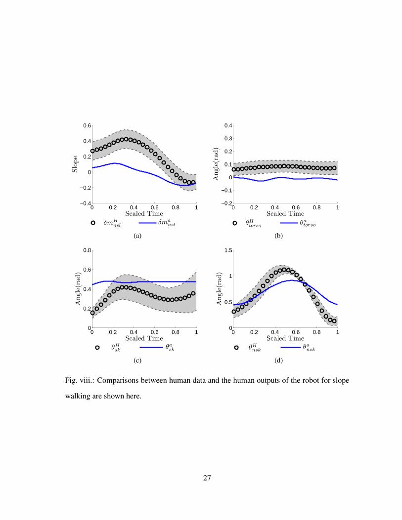
IV.2.2. Walking on a slope

Walking on a slope is obtained by solving the optimization problem for a non-zero value

of the slope angle, γ . We considered a particular value of γ = 20, which is a reasonable

slope for a robot of the size and power capabilities of AMBER. Again, we get α∗γ , the

solution to the optimization problem and apply the voltage control law resulting in stable

up-slope walking. The periodic orbit for the walking obtained is shown in Fig. vii. A

comparison between the human output data and simulated robot output data is shown in

Fig. viii. Considering the fact that the slope 20 is small, it is fair to compare the simulated

outputs with flat ground walking data from humans. Fig. ix shows the comparison between

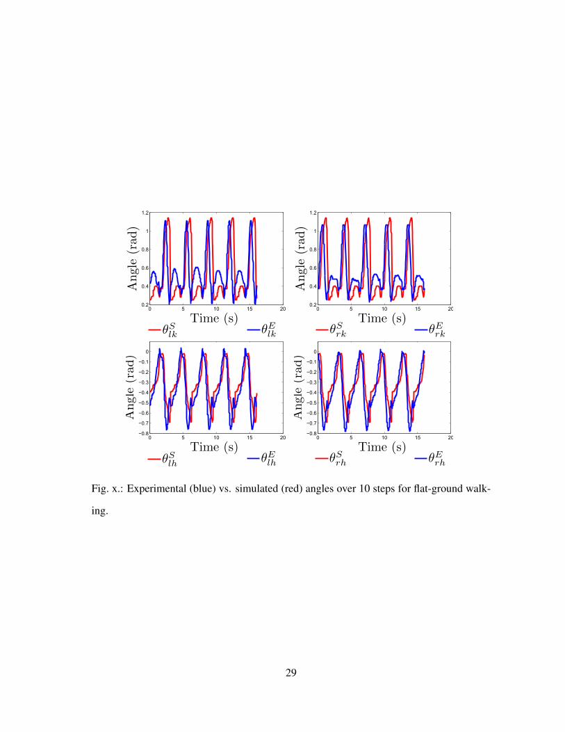
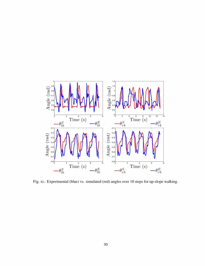
the simulated and experimental tiles for both flat-ground and up-slope walking. Fig. x and

Fig. xi show how well the outputs of the robot track the actual outputs obtained from the

CWF for flat-ground and up-slope walking respectively.

23

−0.5 0 0.5 1

−3

−2

−1

0

1

2

Angle (rad)

Angu

lar

Vel

ocity

(rad

s/s)

Periodic Orbit - Voltage Control

θsf θsk θsh

θnsh θnsk

(a)

0 0.2 0.4 0.6 0.8 1 1.2

−0.2

0

0.2

0.4

0.6

0.8

1

1.2

Time (s)

Joi

ntA

ngl

es(r

ad)

Joint angles - Voltage Control

θsf θsk θsh

θnsh θnsk

(b)

0 0.2 0.4 0.6 0.8 1 1.2−4

−3

−2

−1

0

1

2

3

Time (s)

Tor

que

(N-m

)

Torque Variation-Voltage Control

usk ush unsh

unsk

(c)

0 0.2 0.4 0.6 0.8 1 1.2

−10

−5

0

5

Time (s)

Vol

tage

(V)

Voltage Variation-Voltage Control

Vnsl Vsk Vnsk

Vtor

(d)

(e)

Fig. v.: Phase portrait of the walking gait is shown in (a), joint angles are shown in (b),

variation of torques acting with time are shown in (c), variation of voltages with time are

shown in (d) and the walking tile is shown in (e).

24

0 0.2 0.4 0.6 0.8 1

−0.2

0

0.2

0.4

Scaled Time

Slo

pe

Voltage Control

δmHnsl

δmansl

(a)

0 0.2 0.4 0.6 0.8 1−0.2

−0.1

0

0.1

0.2

0.3

0.4

Scaled TimeA

ngle

(rad)

Voltage Control

θHtorso θa

torso

(b)

0 0.2 0.4 0.6 0.8 10

0.2

0.4

0.6

0.8

Scaled Time

Angle

(rad)

Voltage Control

θHsk

θask

(c)

0 0.2 0.4 0.6 0.8 10

0.2

0.4

0.6

0.8

1

1.2

Scaled Time

Angle

(rad)

Voltage Control

θHnsk

θansk

(d)

Fig. vi.: Comparisons between human data and the human outputs of the robot for flat-

ground walking are shown here.

25

−0.6 −0.4 −0.2 0 0.2 0.4 0.6 0.8

−6

−4

−2

0

2

4

6

8

Angle (rad)

Angu

lar

Vel

ocity

(rad

s/s)

Periodic Orbit - With slope, γ = 20

θsf θsk θsh

θnsh θnsk

(a)

0 0.05 0.1 0.15−0.6

−0.4

−0.2

0

0.2

0.4

0.6

0.8

Time (s)

Joi

ntA

ngl

es(r

ad)

Joint angles - With slope, γ = 20

θsf θsk θsh

θnsh θnsk

(b)

0 0.05 0.1 0.15

−15

−10

−5

0

5

Time (s)

Tor

que

(N-m

)

Torque Variation - With slope, γ = 20

usk ush unsh

unsk

(c)

0 0.05 0.1 0.15

−30

−20

−10

0

10

20

Time (s)

Vol

tage

(V)

Voltage Variation - With slope, γ = 20

Vnsl Vsk Vnsk

Vtor

(d)

(e)

Fig. vii.: Phase portrait of the walking gait is shown in (a), joint angles are shown in (b),

variation of torques acting with time are shown in (c), variation of voltages with time are

shown in (d) and the walking tile is shown in (e).

26

0 0.2 0.4 0.6 0.8 1−0.4

−0.2

0

0.2

0.4

0.6

Scaled Time

Slo

pe

δmHnsl

δmansl

(a)

0 0.2 0.4 0.6 0.8 1−0.2

−0.1

0

0.1

0.2

0.3

0.4

Scaled TimeA

ngle

(rad)

θHtorso θa

torso

(b)

0 0.2 0.4 0.6 0.8 10

0.2

0.4

0.6

0.8

Scaled Time

Angle

(rad)

θHsk

θask

(c)

0 0.2 0.4 0.6 0.8 10

0.5

1

1.5

Scaled Time

Angle

(rad)

θHnsk

θansk

(d)

Fig. viii.: Comparisons between human data and the human outputs of the robot for slope

walking are shown here.

27

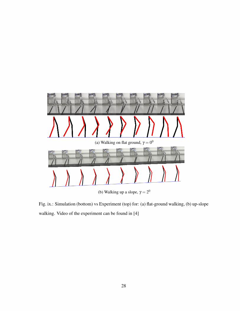
(a) Walking on flat ground, γ = 00

(b) Walking up a slope, γ = 20

Fig. ix.: Simulation (bottom) vs Experiment (top) for: (a) flat-ground walking, (b) up-slope

walking. Video of the experiment can be found in [4]

28

0 5 10 15 200.2

0.4

0.6

0.8

1

1.2

Time (s)

Angl

e(r

ad)

θSlk

θElk

0 5 10 15 200.2

0.4

0.6

0.8

1

1.2

Time (s)

Angl

e(r

ad)

θSrk

θErk

0 5 10 15 20−0.8

−0.7

−0.6

−0.5

−0.4

−0.3

−0.2

−0.1

0

Time (s)

Angl

e(r

ad)

θSlh

θElh

0 5 10 15 20−0.8

−0.7

−0.6

−0.5

−0.4

−0.3

−0.2

−0.1

0

Time (s)

Angl

e(r

ad)

θSrh

θErh

Fig. x.: Experimental (blue) vs. simulated (red) angles over 10 steps for flat-ground walk-

ing.

29

0 2 4 6 8

0.4

0.5

0.6

0.7

0.8

0.9

1

Time (s)

Angl

e(r

ad)

θSlk

θElk

0 2 4 6 8 10 12 140

0.2

0.4

0.6

0.8

1

1.2

1.4

Time (s)

Angl

e(r

ad)

θSrk

θErk

0 2 4 6 8−0.8

−0.7

−0.6

−0.5

−0.4

−0.3

−0.2

−0.1

Time (s)

Angl

e(r

ad)

θSlh

θElh

0 2 4 6 8−0.8

−0.7

−0.6

−0.5

−0.4

−0.3

−0.2

−0.1

Time (s)

Angl

e(r

ad)

θSrh

θErh

Fig. xi.: Experimental (blue) vs. simulated (red) angles over 10 steps for up-slope walking.

30

CHAPTER V

WALKING ON ROUGH TERRAIN

This section will introduce the methods adopted to achieve Hybrid Zero Dynamics on rough

terrain. On flat ground, the zero dynamics surface (Zα ) derived from the CWF (α) is

respected i.e., the robot will exhibit Hybrid Zero Dynamics. But, on an uneven terrain, i.e.,

when the non-stance foot hits the ground at a height hR 6= 0, then the resulting post-impact

state, x+ = (θ+, θ+), may not be on the same surface. This calls for defining a new set of

CWF in such a way that the post-impact state of the robot resides on the resulting new zero

dynamics surface (call it the intermediate zero dynamics surface, Zαint). This effectively

reduces the problem to finding the new CWF, the resulting intermediate zero dynamics

surface of which contains the post-impact state. Given the post-impact state obtained due

the non-zero height(hR) of non-stance foot, x+, we find the new CWF by computing the

new set of parameters of walking, α int .

V.1. Extended Canonical Walking Function (ECWF) and Intermediate Motion Transi-

tions (IMT)

Given the canonical walking function in (5.4), we have the robot outputs and their deriva-

tives:

ya(θ+) = Hθ

+, dya(θ+) =

Hθ+

ξ+1

, (5.1)

where ξ+1 = cθ+ (from (3.11)) is the post-impact hip velocity and dya is effectively the

derivative of the outputs divided by the post-impact hip velocity. The reason for dividing

by the hip velocity is to make the outputs independent of the joint angle velocities and

31

based on the fact that if HZD is respected for one point on the guard, then it must be

respected for all the points on the zero dynamics surface. This is proved in [29] for the case

of underactuated walking.

We can design α int in such a way that it brings the state of the robot back to the zero

dynamics surface for flat ground walking. To be more precise, if the next step were to be

flat (hR = 0), then the intermediate surface, Zαint , will lead the state of the robot back to the

original surface Zα . In other words, the construction of α int will allow the guard of Zαint

to intersect with the guard of Zα .

The end of the step for flat ground walking, x− = (θ−, θ−), can be computed from,

x− = (θ(ϑ(α)), θ(ϑ(α))). The corresponding outputs and their derivatives are:

ya(θ−) = Hθ

−, dya(θ−) =

Hθ−

ξ−1

, (5.2)

with ξ−1 = cθ− being the hip velocity at the end of the step (again, the end of this interme-

diate step is assumed to be on flat ground).

Since the desired outputs should equal the outputs of the robot to ensure hybrid invari-

ance, the goal will be to find α int for which the following is satisfied:

ya(θ+) = yd(τ(θ

+),α int), dya(θ+) =

∂yd(τ(θ+),α int)

∂ξ+1

,

ya(θ−) = yd(τ(θ

−),α int), dya(θ+) =

∂yd(τ(θ−),α int)

∂ξ−1

, (5.3)

where τ is the time parameterized by hip position given in (3.6).

Since there are four outputs, and ya(θ)∈R4, (5.3) has 16 equations with the unknown

being α int ∈ R21. Due the way the CWF was constructed, finding a solution (or one of

the solutions) to the 16 nonlinear complex equations will be time consuming and may not

be guaranteed. This motivates introducing a new function called the extended canonical

32

walking function (ECWF):

yHe(t,α) = e−α4t(α1 cos(α2t)+α3 sin(α2t))+α5 cos(α6t)+

2α5α4α2

α22 +α2

4 −α26

sin(α6t)+α7, (5.4)

which has seven parameters and four of the parameters can be written in vector form,

αv = [α1,α3,α5, α7]T which are linear in the expression and can be separated out in the

following manner:

LTV (t,α) =

e−α4t cos(α2t),

e−α4t sin(α2t),

cos(α6t)+ 2α4α6α2

2+α24−α2

6sin(α6t),

1

,

yHe(t,α) = LTV T (t,α)αv, (5.5)

where LTV is the linear transformation vector containing the remaining expression which

becomes a constant vector by keeping α2,α4,α6 constant. Similarly, we can define the

partial derivative of the desired extended outputs:

LTVd(t,α) =

−α4e−α4t cos(α2t)−α2e−α4t sin(α2t),

−α4e−α4t sin(α2t)+α2e−α4t cos(α2t),

−α6 sin(α6t)+ 2α4α26

α22+α2

4−α26

cos(α6t),

0

,

dyHe(t,α) =∂yHe(t,α)

∂ξ1= LTV T

d (t,α)∂ t

∂ξ1αv. (5.6)

LTVd is the time derivative of LTV ; and from (3.6) and (3.11), it follows that ∂ t∂ξ1

= v−1hip.

33

We can now use the ECWF, to replace (3.5) with:

yde(τ,α) =

yHe(τ,αnsl)

yHe(τ,αsk)

yHe(τ,αnsk)

yHe(τ,αtor)

,

∂yde(τ,α)

∂ξ1=

dyHe(τ,αnsl)

dyHe(τ,αsk)

dyHe(τ,αnsk)

dyHe(τ,αtor)

, (5.7)

which is obtained from the new set of parameters, α = (vhip,αnsl,αsk,αnsk,αtor) ∈ R29.

Accordingly, the new desired outputs (5.7) will replace the desired outputs in (5.3) resulting

in 16 linear equations with 29 unknowns. Note that control law in (3.8) will bear no change

with yd replaced with yde and the hybrid invariance will still be valid. By keeping vhip and

α2,α4,α6 of all outputs constant, (5.3) will contain 16 unknowns, and can be solved for

in a straightforward manner. To illustrate, we will consider one of the outputs, the stance

knee angle, θsk, resulting in:

ysk(θ+) = θ

+sk , dysk(θ

+) =θ+sk

ξ+1

,

ysk(θ−) = θ

−sk , dysk(θ

−) =θ−sk

ξ−1

, (5.8)

and (5.3) yields:

ysk(θ+) = yHe(τ(θ

+),α intsk ), dysk(θ

+) = dyHe(τ(θ+),α int

sk ),

ysk(θ−) = yHe(τ(θ

−),α intsk ), dysk(θ

−) = dyHe(τ(θ−),α int

sk ). (5.9)

34

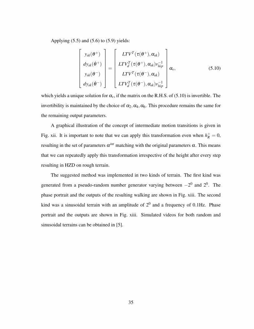
Applying (5.5) and (5.6) to (5.9) yields:

ysk(θ+)

dysk(θ+)

ysk(θ−)

dysk(θ−)

=

LTV T (τ(θ+),αsk)

LTV Td (τ(θ+),αsk)v−1

hip

LTV T (τ(θ−),αsk)

LTV Td (τ(θ−),αsk)v−1

hip

αv, (5.10)

which yields a unique solution for αv, if the matrix on the R.H.S. of (5.10) is invertible. The

invertibility is maintained by the choice of α2,α4,α6. This procedure remains the same for

the remaining output parameters.

A graphical illustration of the concept of intermediate motion transitions is given in

Fig. xii. It is important to note that we can apply this transformation even when h+R = 0,

resulting in the set of parameters α int matching with the original parameters α . This means

that we can repeatedly apply this transformation irrespective of the height after every step

resulting in HZD on rough terrain.

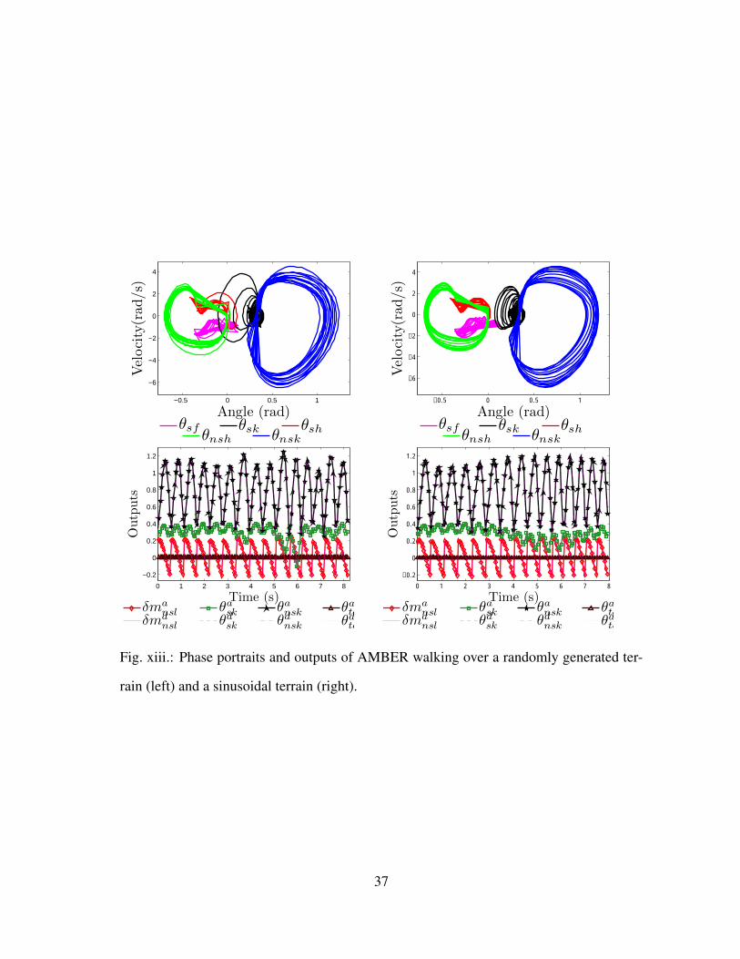
The suggested method was implemented in two kinds of terrain. The first kind was

generated from a pseudo-random number generator varying between −20 and 20. The

phase portrait and the outputs of the resulting walking are shown in Fig. xiii. The second

kind was a sinusoidal terrain with an amplitude of 20 and a frequency of 0.1Hz. Phase

portrait and the outputs are shown in Fig. xiii. Simulated videos for both random and

sinusoidal terrains can be obtained in [5].

35

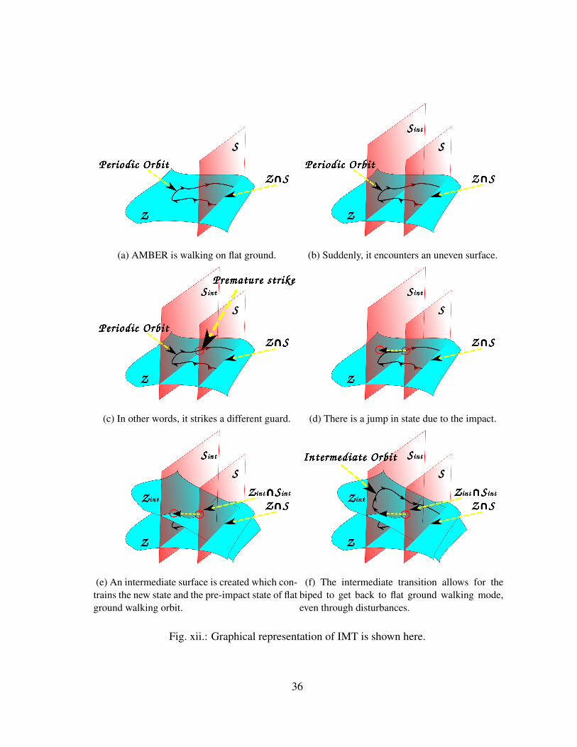
(a) AMBER is walking on flat ground. (b) Suddenly, it encounters an uneven surface.

(c) In other words, it strikes a different guard. (d) There is a jump in state due to the impact.

(e) An intermediate surface is created which con-trains the new state and the pre-impact state of flatground walking orbit.

(f) The intermediate transition allows for thebiped to get back to flat ground walking mode,even through disturbances.

Fig. xii.: Graphical representation of IMT is shown here.

36

−0.5 0 0.5 1

−6

−4

−2

0

2

4

Angle (rad)

Vel

oci

ty(r

ad/s)

Periodic Orbit - Random Ter

θsf θsk θsh

θnsh θnsk

−0.5 0 0.5 1

−6

−4

−2

0

2

4

Angle (rad)Vel

oci

ty(r

ad/s)

θsf θsk θsh

θnsh θnsk

0 1 2 3 4 5 6 7 8

−0.2

0

0.2

0.4

0.6

0.8

1

1.2

Time (s)

Outp

uts

δmansl θa

sk θansk θa

to

δmdnsl θd

sk θdnsk θd

to

0 1 2 3 4 5 6 7 8

−0.2

0

0.2

0.4

0.6

0.8

1

1.2

Time (s)

Outp

uts

δmansl θa

sk θansk θa

to

δmdnsl θd

sk θdnsk θd

to

Fig. xiii.: Phase portraits and outputs of AMBER walking over a randomly generated ter-

rain (left) and a sinusoidal terrain (right).

37

V.2. Experimental Implementation of IMT

AMBER is powered by DC motors, and therefore the type of control law suggested in

(3.8) requires knowing the model parameters of the robot. Instead, by looking at the joint

angles obtained from the absolute encoders, we adopted a simple linear control law: Vin =

−Kpyα(θ), Vin is the vector of voltage inputs to the motors and Kp is the proportional

constant. More details can be found in [30].

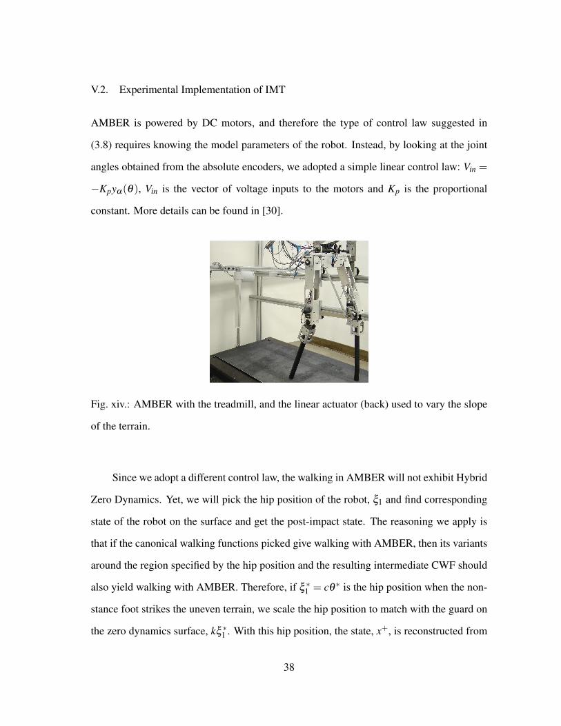
Fig. xiv.: AMBER with the treadmill, and the linear actuator (back) used to vary the slope

of the terrain.

Since we adopt a different control law, the walking in AMBER will not exhibit Hybrid

Zero Dynamics. Yet, we will pick the hip position of the robot, ξ1 and find corresponding

state of the robot on the surface and get the post-impact state. The reasoning we apply is

that if the canonical walking functions picked give walking with AMBER, then its variants

around the region specified by the hip position and the resulting intermediate CWF should

also yield walking with AMBER. Therefore, if ξ ∗1 = cθ ∗ is the hip position when the non-

stance foot strikes the uneven terrain, we scale the hip position to match with the guard on

the zero dynamics surface, kξ ∗1 . With this hip position, the state, x+, is reconstructed from

38

the zero dynamics surface by using (3.13):

x+ = ∆

Φ(kξ ∗1 )

∂Φ(kξ ∗1 )∂ξ1

vhip

, (5.11)

where ∆ gives the post-impact map from the reconstructed state. Accordingly, the inter-

mediate transition matrix is obtained as described in Section V. It is important to note that

this transition matrix is dynamically updated in AMBER after every non-stance foot strike.

The sinusoidal terrain is created by sinusoidally exciting the linear actuator connecting the

treadmill (see Fig. xiv). Tiles of AMBER walking over a rough terrain for one step are

shown in Fig. xv and Fig. xvi shows the variation of outputs of the robot on the sinusoidal

terrain (see video [3]). Fig. xvii shows all the ECWF computed from the updated α int after

every step, and they are compared with the human data.

39

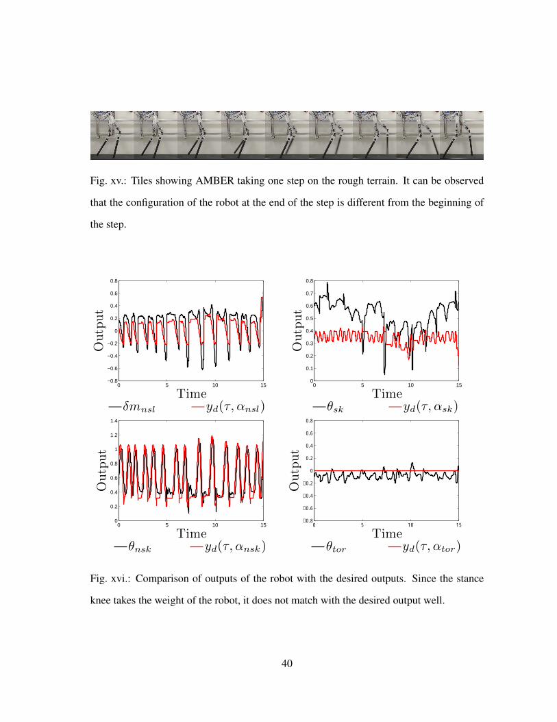
Fig. xv.: Tiles showing AMBER taking one step on the rough terrain. It can be observed

that the configuration of the robot at the end of the step is different from the beginning of

the step.

0 5 10 15−0.8

−0.6

−0.4

−0.2

0

0.2

0.4

0.6

0.8

Time

Outp

ut

δmnsl

yd(τ, αnsl)

0 5 10 150

0.1

0.2

0.3

0.4

0.5

0.6

0.7

0.8

Time

Outp

ut

θsk

yd(τ, αsk)

0 5 10 150

0.2

0.4

0.6

0.8

1

1.2

1.4

Time

Outp

ut

θnsk

yd(τ, αnsk)

0 5 10 15−0.8

−0.6

−0.4

−0.2

0

0.2

0.4

0.6

0.8

Time

Outp

ut

θtor

yd(τ, αtor)

Fig. xvi.: Comparison of outputs of the robot with the desired outputs. Since the stance

knee takes the weight of the robot, it does not match with the desired output well.

40

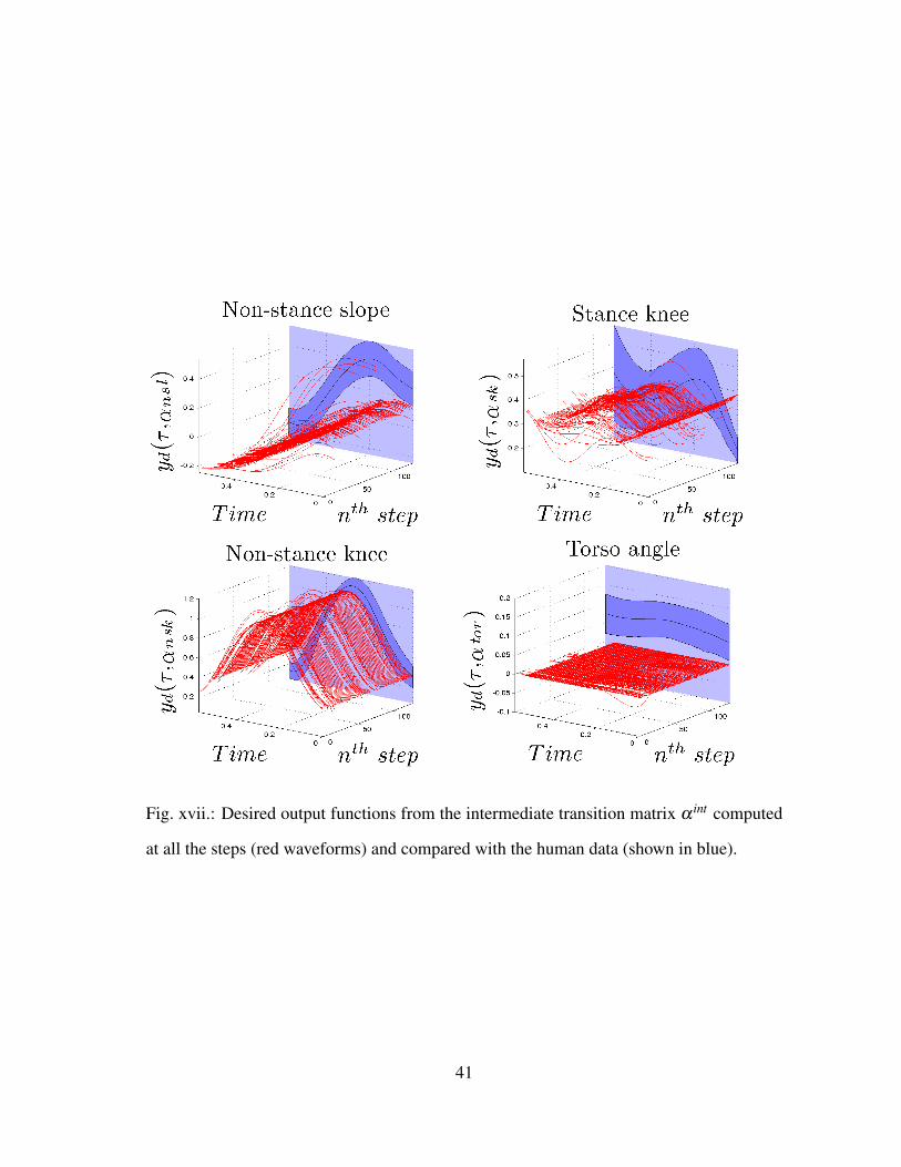
Fig. xvii.: Desired output functions from the intermediate transition matrix α int computed

at all the steps (red waveforms) and compared with the human data (shown in blue).

41

CHAPTER VI

CONCLUSIONS

This thesis successfully achieved walking on three motion primitives by using human-

inspired control which is not only stable, but also remarkably robust (see video [1]). From

walking tiles and joint angle tracking behavior considered, it can be stated that the physi-

cally realizable walking obtained from the simulation is mirrored in the walking obtained in

physical world. This speaks a lot about the strength of the formal theory on human-inspired

control. In fact, the walking was achieved with minimal computation overhead requiring

less than 100 lines of code in LabVIEW. One of the reasons that can be attributed to the

success is the choice of the CWF chosen. The fact that human walking is an end product

of thousands of years of evolution, and that the robustness is inherently built into human

walking, shows the extent to which AMBER can be pushed and still walk stably on the

platform. It must also be stressed that the feet are not actuated, which makes the problem

to realize natural human-like motion primitives even harder. The concept of using motion

transitions made the walking even more robust, resulting in stable walking even on an un-

known random terrain. The application of the computation for rough terrain transitions is

limited by the maximum height at which the robot hits the ground. In other words, since

we are using one reference CWF, the time parameter τ+ must be within the limits to realize

the transformation. The limits are decided by the restriction on hyper extension of the knee

and also the maximum achievable speed on the robot. For the canonical walking function

that was picked for AMBER, 0.532 < τ+ < 0.574. With the transformation suggested and

with the limits specified, preliminary experiments showed significant improvement in the

walking obtained. Since, the intermediate walking functions yield different steady state

walking speeds with the robot, it will move backward and forward w.r.t. the treadmill

42

which is set at constant speed. Inspite of that, the improvement in walking is observed,

thereby justifying the application of intermediate motion transitions. The ability to obtain

provably stable walking gaits in the simulation and then translate it in the form of propor-

tional voltage controller in AMBER establishes a delicate and yet reliable nexus between

theory and experiment, which inscribes the formula for success.

43

REFERENCES

[1] AMBER robustness tests.

http://youtu.be/RgQ8atV1NW0.

[2] Human-Inspired Proportional Control with AMBER in simulation.

http://www.youtube.com/watch?v=z3oPzlStzRo.

[3] Motion transitions up the slope and on a sinusoidal terrain.

http://youtu.be/aUiEXt8otrY.

[4] Robust walking of amber on flat-ground and up-slope.

http://www.youtube.com/watch?v=aBfszNZs5mQ.

[5] Simulated walking on random and sinusoidal terrains.

http://youtu.be/OtW1I4kRWj8

http://youtu.be/p7bdqmYhzcc.

[6] A. D. Ames. First steps toward automatically generating bipedal robotic walking

from human data. In Robotic Motion and Control 2011, volume 422 of LNICS, pages

89–116. Springer, 2012.

[7] A. D. Ames. First steps toward underactuated human-inspired bipedal robotic walk-

ing. In 2012 IEEE Conference on Robotics and Automation, St. Paul, Minnesota,

2012.

[8] A. D. Ames, E. A. Cousineau, and M. J. Powell. Dynamically stable robotic walking

with NAO via human-inspired hybrid zero dynamics. In Hybrid Systems: Computa-

tion and Control, 2012, Beijing, China, 2012.

44

[9] A. D. Ames, R. Vasudevan, and R. Bajcsy. Human-data based cost of bipedal robotic

walking. In Hybrid Systems: Computation and Control, Chicago, IL, 2011.

[10] T. Burg, D. Dawson, J. Hu, and M. de Queiroz. An adaptive partial state-feedback

controller for RLED robot manipulators. IEEE Transactions on Automatic Control,

41(7):1024 –1030, 1996.

[11] K. Byl and R. Tedrake. Metastable walking machines. International Journal of

Robotics Research, 28(8):1040 – 1064, Aug 2009.

[12] S. Collins, A. Ruina, R. Tedrake, and M. Wisse. Efficient bipedal robots based on

passive-dynamic walkers. Science, 307:1082–1085, 2005.

[13] H. Geyer and H. Herr. A muscle-reflex model that encodes principles of legged me-

chanics produces human walking dynamics and muscle activities. IEEE Transactions

on Neural Systems and Rehabilitation Engineering, 18(3):263 –273, 2010.

[14] J. W. Grizzle, J. Hurst, B. Morris, H. Park, and K. Sreenath. MABEL, a new robotic

bipedal walker and runner. In American Control Conference, pages 2030–2036, St.

Louis, MO, USA, 2009.

[15] P. Holmes, R. J. Full, D. Koditschek, and J. Guckenheimer. The dynamics of legged

locomotion: Models, analyses, and challenges. SIAM Rev., 48:207–304, 2006.

[16] A. J. Ijspeert. Central pattern generators for locomotion control in animals and robots:

a review. Neural Networks, 21(4):642–653, 2008.

[17] C. Liu, C. C. Cheah, and J. E. Slotine. Adaptive jacobian tracking control of rigid-

link electrically driven robots based on visual task-space information. Automatica,

42(9):1491 – 1501, 2006.

45

[18] I. R. Manchester, U. Mettin, F. Iida, and R. Tedrake. Stable dynamic walking over un-

even terrain. The International Journal of Robotics Research, 30(3):265–279, 2011.

[19] T. McGeer. Passive dynamic walking. Intl. J. of Robotics Research, 9(2):62–82, April

1990.

[20] R. M. Murray, Zexiang Li, and S. S. Sastry. A Mathematical Introduction to Robotic

Manipulation. CRC Press, Boca Raton, 1994.

[21] J. Bo. Nielsen. How we walk : Central control of muscle activity during human

walking. The Neuroscientist, 9(3):195–204, 2003.

[22] H. Park, K. Sreenath, J. Hurst, and J. W. Grizzle. Identification of a bipedal robot

with a compliant drivetrain: Parameter estimation for control design. IEEE Control

Systems Magazine, 31(2):63–88, 2011.

[23] I. Poulakakis and J. W. Grizzle. The Spring Loaded Inverted Pendulum as the Hy-

brid Zero Dynamics of an Asymmetric Hopper. Transaction on Automatic Control,

54(8):1779–1793, 2009.

[24] M. H. Raibert. Legged robots. Communications of the ACM, 29(6):499–514, 1986.

[25] S. S. Sastry. Nonlinear Systems: Analysis, Stability and Control. Springer, New

York, 1999.

[26] R. Sinnet, M. Powell, R. Shah, and A. D. Ames. A human-inspired hybrid control

approach to bipedal robotic walking. In 18th IFAC World Congress, Milano, Italy,

2011.

[27] M. W. Spong. Passivity based control of the compass gait biped. In IFAC World

Congress, Beijing, 1999.

46

[28] S. Srinivasan, I. A. Raptis, and E. R. Westervelt. Low-dimensional sagittal plane

model of normal human walking. ASME J. of Biomechanical Eng., 130(5), 2008.

[29] E. R. Westervelt, J. W. Grizzle, C. Chevallereau, J. H. Choi, and B. Morris. Feedback

Control of Dynamic Bipedal Robot Locomotion. CRC Press, Boca Raton, 2007.

[30] S. Nadubettu Yadukumar, M. Pasupuleti, and A. D. Ames. From formal methods to

algorithmic implementation of human inspired control on bipedal robots. In Tenth

International Workshop on the Algorithmic Foundations of Robotics (WAFR), Cam-

bridge, MA, 2012.

[31] S. Nadubettu Yadukumar, M. Pasupuleti, and A. D. Ames. Human-inspired under-

actuated bipedal robotic walking with amber on flat-ground, up-slope and uneven

terrain. In IEEE/RSJ International Conference on Intelligent Robots and Systems

(IROS), Algarve, Portugal, 2012.

47