Embed Size (px)
Citation preview

Bipartite Graphs as Models of ComplexNetworks
Jean-Loup Guillaume and Matthieu Latapyliafa – cnrs – Universite Paris 7
2 place Jussieu, 75005 Paris, France.(guillaume,latapy)@liafa.jussieu.fr
Abstract
It appeared recently that the classical random graph model usedto represent real-world complex networks does not capture their mainproperties. Since then, various attempts have been made to provideaccurate models. We study here the first model which achieves thefollowing challenges: it produces graphs which have the three mainwanted properties (clustering, degree distribution, average distance),it is based on some real-world observations, and it is sufficiently simpleto make it possible to prove its main properties. This model consistsin sampling a random bipartite graph with prescribed degree distri-bution. Indeed, we show that any complex network can be viewed asa bipartite graph with some specific characteristics, and that its mainproperties can be viewed as consequences of this underlying structure.We also propose a growing model based on this observation.
Introduction.
When one wants to model a real-world object (in the sense of producing anartificial object similar to the real one), one first has to get some informationon its properties, generally using a measurement procedure and an analysisof the result of this measure. There are then basically two ways to proposea model.
First, one may consider a set of observed properties as essential, and thensample randomly objects among the ones which have these properties. Oneobtains this way a typical object with the properties in concern. It is then
1
possible to determine if the retained set of properties is sufficient (do therandom objects produced by the model fit well the real one?) and to studythe expected behavior of the object of interest. The relevance of the set ofproperties is generally checked using other known properties or behaviors ofthe object.
The other modeling approach is to define a construction process inspiredfrom the way the object is really constructed. This construction process isgenerally iterated from an initial state, and eventually leads to an appropriateobject. The analysis then concerns the properties induced by the constructionprocess: do they fit real-world properties?
The first method is in general more suitable for analysis, and more rig-orous, but it may be very difficult to sample a random object in a givenclass. On the opposite, the second approach generally gives a simple sam-pling scheme and has the advantage of producing evolving objects. But theconstruction process may induce some properties which do not correspondto any reality, and is in general difficult to analyze.
It has been shown recently that most real-world complex networks havesome essential properties in common. These properties are not captured bythe model generally used before this discovery, although they play a centralrole in many contexts like the robustness of the Internet [6, 19, 20, 15, 49],the spread of viruses or rumors over the Internet, the Web or other socialnetworks [48, 52, 58], as well as the performance of protocols and algorithms[36, 41, 63].
This is why, in the last few years, a strong effort has been put in the real-istic modeling of complex networks, both in computer science, mathematicsand physics, and much progress has been accomplished in this field. Somemodels achieve the aim of producing graphs which capture some, but not allof the main properties of real-world complex networks. Some models obtainall the wanted properties but rely on artificial methods which give unrealisticgraphs (trees, graphs with uniform degrees, etc). Others rely on constructionprocesses which may induce some hidden properties, or are too difficult toanalyze.
In this paper, we propose the random bipartite graph model as a generalmodel for complex networks. It has all the advantages we have just cited,without the drawbacks. It produces graphs with all the wanted properties.It relies on real-world observations and gives realistic graphs. Finally, it issimple enough to make it possible to prove its main properties.
We will first present an overview of the context in which our work lies.In particular, we use some ideas introduced in previous papers, which weneed to describe precisely. Then we show how all complex networks may be
2
described as bipartite structures. After this, we present the random bipartitemodel and analyze it to show that the main properties of complex networksare somehow a consequence of their underlying bipartite structure. We alsopresent a growing bipartite model based on the same ideas. Finally we discussthe advantages and limitations of these models.
1 Context.
Throughout our presentation, we will use a representative set of complexnetworks which have received much attention and span quite well the varietyof contexts in which complex networks appear. These complex networkscan be divided in three main classes, namely social networks, technologicalnetworks and biological ones. The set consists of:
• Internet. The interconnection of routers (or AS) on the Internet canbe modeled by graphs where the nodes are routers (or groups of routers)linked with physical links. We use several graphs from [16, 32, 33]
• Web. The hyperlinks between Web pages give a natural graph struc-ture to the World Wide Web [14, 37]. We will use here the Notre DameWeb graph from [5, 23].
• Cooccurrence. When one considers a book, or the queries to a searchengine, or a chat on an interactive system for instance, one can con-struct a co-occurrence graph by linking two words if they appear in thesame sentence or query [31]. Here, we will use a version of the Bible[62].
• Actors. In this social network, two actors are connected if they haveplayed together in a movie. This graph is widely studied for manyreasons: it is very large, well representative of social networks, evolv-ing with each new movie produced, and easily available through theInternet Movie Database [24, 64].
• Coauthoring. Another way to link people is according to their scien-tific publications: two scientists are linked if they have signed a papertogether [50, 51, 56]. We will use such a graph obtained from the LosAlamos preprint archive [7].
• Proteins. In [35] the authors link together two proteins of a givenbiological system if they influence each other. We will consider thisexample too, using graphs from [23].
3
Many other complex networks have been studied. Refer to [4, 26, 54] fora more descriptive list of networks and corresponding references. All thesenetworks have some properties in common which have been discovered quiterecently and have concentrated a large attention in various communities.Hereafter we present the properties in concern and some recent efforts in themodeling of these properties.
1.1 Statistical properties
Most real-world complex networks have a number of edges m which scaleslinearly with the number of vertices n: m ∼ k · n where k is the averagedegree (which does not depend on the size of the graph). Therefore, thesenetworks have a low density (going to 0 when n grows), the density beingdefined as the number of existing edges over the number of edges that couldexist.
Three other properties received recently much attention due to the factthat they have unexpected behaviors in real-world complex networks: theaverage distance between vertices, the clustering and the degree distribution.
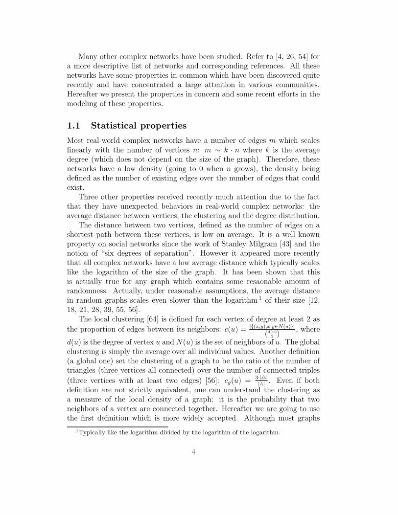
The distance between two vertices, defined as the number of edges on ashortest path between these vertices, is low on average. It is a well knownproperty on social networks since the work of Stanley Milgram [43] and thenotion of “six degrees of separation”. However it appeared more recentlythat all complex networks have a low average distance which typically scaleslike the logarithm of the size of the graph. It has been shown that thisis actually true for any graph which contains some resaonable amount ofrandomness. Actually, under reasonable assumptions, the average distancein random graphs scales even slower than the logarithm 1 of their size [12,18, 21, 28, 39, 55, 56].
The local clustering [64] is defined for each vertex of degree at least 2 as
the proportion of edges between its neighbors: c(u) = |{(x,y),x,y∈N(u)}|(d(u)
2 ), where
d(u) is the degree of vertex u and N(u) is the set of neighbors of u. The globalclustering is simply the average over all individual values. Another definition(a global one) set the clustering of a graph to be the ratio of the number oftriangles (three vertices all connected) over the number of connected triples
(three vertices with at least two edges) [56]: cg(u) = 3·|4||∧| . Even if both
definition are not strictly equivalent, one can understand the clustering asa measure of the local density of a graph: it is the probability that twoneighbors of a vertex are connected together. Hereafter we are going to usethe first definition which is more widely accepted. Although most graphs
1Typically like the logarithm divided by the logarithm of the logarithm.
4
Internet Web Actors Co-auth Co-occur Protein
n 75885 325729 392340 16401 9297 2113
m 357317 1090108 15038083 29552 392066 2203
density 1.2e-4 2.1e-5 1.9e-4 2.2e-4 9.1e-3 9.9e-4
α 2.5 2.3 2.2 2.4 1.8 2.4
c 0.171 0.466 0.785 0.638 0.822 0.153
d 5.80 7 3.6 7.18 2.13 6.74
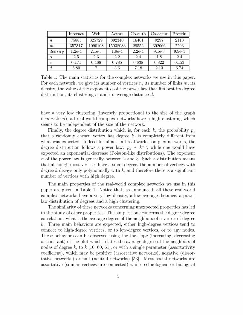
Table 1: The main statistics for the complex networks we use in this paper.For each network, we give its number of vertices n, its number of links m, itsdensity, the value of the exponent α of the power law that fits best its degreedistribution, its clustering c, and its average distance d.
have a very low clustering (inversely proportional to the size of the graphif m ∼ k · n), all real-world complex networks have a high clustering whichseems to be independent of the size of the network.
Finally, the degree distribution which is, for each k, the probability pkthat a randomly chosen vertex has degree k, is completely different fromwhat was expected. Indeed for almost all real-world complex networks, thedegree distribution follows a power law: pk ∼ k−α, while one would haveexpected an exponential decrease (Poisson-like distributions). The exponentα of the power law is generally between 2 and 3. Such a distribution meansthat although most vertices have a small degree, the number of vertices withdegree k decays only polynomially with k, and therefore there is a significantnumber of vertices with high degree.
The main properties of the real-world complex networks we use in thispaper are given in Table 1. Notice that, as announced, all these real-worldcomplex networks have a very low density, a low average distance, a powerlaw distribution of degrees and a high clustering.
The similarity of these networks concerning unexpected properties has ledto the study of other properties. The simplest one concerns the degree-degreecorrelation: what is the average degree of the neighbors of a vertex of degreek. Three main behaviors are expected, either high-degree vertices tend toconnect to high-degree vertices, or to low-degree vertices, or to any nodes.These behaviors can be observed using the the slope (increasing, decreasingor constant) of the plot which relates the average degree of the neighbors ofnodes of degree k, to k [10, 60, 61], or with a single parameter (assortativitycoefficient), which may be positive (assortative networks), negative (dissor-tative networks) or null (neutral networks) [53]. Most social networks areassortative (similar vertices are connected) while technological or biological
5
are generally dissortative.One may also correlate the clustering and the degree by computing the
average clustering of vertices having a given degree. This also defines assor-tative (high degree yields high clustering), neutral or dissortative networks.
Finally, other properties have been studied, such as the centrality (howmany shortest paths contain a given vertex) [51], the distribution of eigen-values of the adjacency matrix [30, 42], etc. All these statistical propertiesare used to describe a given complex network and to study the similaritiesand differences between several complex networks. They give precise insighton what one may expect when considering a complex network having a setof properties.
1.2 Modeling complex networks
The basic model for complex networks is the Erdos-Renyi (ER) random graph
model [12, 29]. In a random graph with n vertices, each of the n·(n−1)2
possibleedges exists with a given probability p (this model is know as Gn,p). In anequivalent way when n tends to infinity [12, 29], one may construct such a
random graph from n vertices by choosing m = p · n·(n−1)2
edges at random(Gn,m model).
In such a graph, it is known that the average distance scales with thelogarithm of n [12]. Moreover, the clustering is equal to the connectionprobability p since each pair of vertices is connected with the same probabilityindependently of the fact that they are both linked to a same vertex. Ifm ∼ k · n as in real-world complex networks, this means that the clusteringscales as n−1 and therefore tends to 0 when n grows. Finally, the degreedistribution follows a Poisson law pk ∼ e−λ λ
k
k![12], which implies in particular
that the number of vertices with degree k decays very rapidly around theaverage degree, and therefore all vertices have nearly the same degree.
Therefore, although this model can be considered as relevant concerningthe average distance, it misses the two other main properties of real-worldcomplex networks. In particular, the degree distributions are qualitativelydifferent.
It is however possible to sample uniformly a random graph with a givendegree distribution (in particular a power law) [11, 40, 45, 46] using theMolloy and Reed 2 (MR) model: for each vertex, draw its degree at randomaccording to the given distribution, create as many connection points as its
2Despite it has been introduced in [9] and studied in [11], this model is commonlyrefferred to as the Molloy and Reed model since these authors made it popular in theircontributions [45, 46]. We will follow this convention here.
6
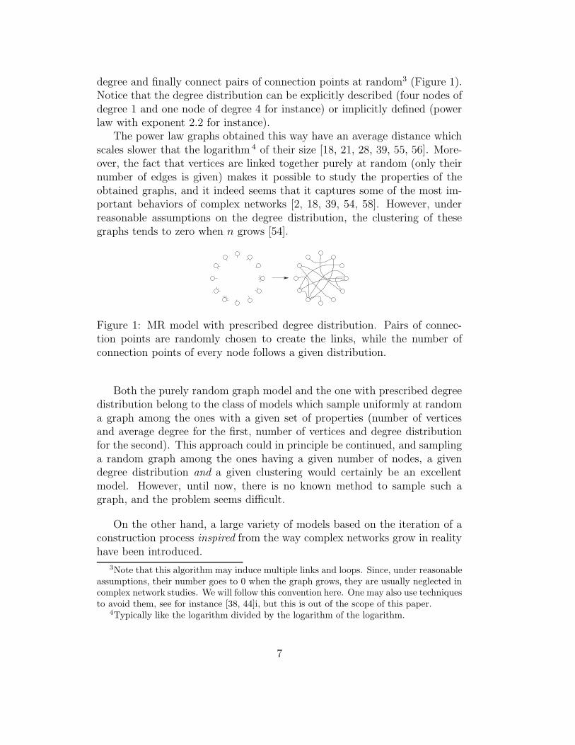
degree and finally connect pairs of connection points at random3 (Figure 1).Notice that the degree distribution can be explicitly described (four nodes ofdegree 1 and one node of degree 4 for instance) or implicitly defined (powerlaw with exponent 2.2 for instance).
The power law graphs obtained this way have an average distance whichscales slower that the logarithm 4 of their size [18, 21, 28, 39, 55, 56]. More-over, the fact that vertices are linked together purely at random (only theirnumber of edges is given) makes it possible to study the properties of theobtained graphs, and it indeed seems that it captures some of the most im-portant behaviors of complex networks [2, 18, 39, 54, 58]. However, underreasonable assumptions on the degree distribution, the clustering of thesegraphs tends to zero when n grows [54].
Figure 1: MR model with prescribed degree distribution. Pairs of connec-tion points are randomly chosen to create the links, while the number ofconnection points of every node follows a given distribution.
Both the purely random graph model and the one with prescribed degreedistribution belong to the class of models which sample uniformly at randoma graph among the ones with a given set of properties (number of verticesand average degree for the first, number of vertices and degree distributionfor the second). This approach could in principle be continued, and samplinga random graph among the ones having a given number of nodes, a givendegree distribution and a given clustering would certainly be an excellentmodel. However, until now, there is no known method to sample such agraph, and the problem seems difficult.
On the other hand, a large variety of models based on the iteration of aconstruction process inspired from the way complex networks grow in realityhave been introduced.
3Note that this algorithm may induce multiple links and loops. Since, under reasonableassumptions, their number goes to 0 when the graph grows, they are usually neglected incomplex network studies. We will follow this convention here. One may also use techniquesto avoid them, see for instance [38, 44]i, but this is out of the scope of this paper.
4Typically like the logarithm divided by the logarithm of the logarithm.
7
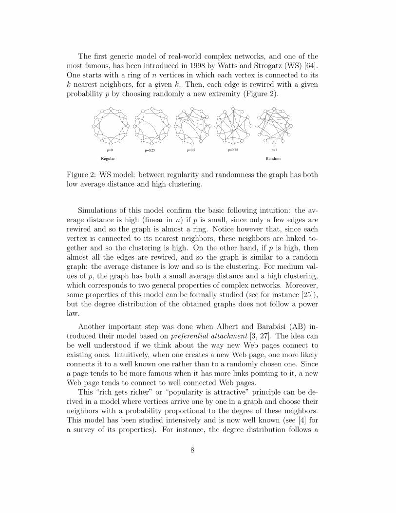
The first generic model of real-world complex networks, and one of themost famous, has been introduced in 1998 by Watts and Strogatz (WS) [64].One starts with a ring of n vertices in which each vertex is connected to itsk nearest neighbors, for a given k. Then, each edge is rewired with a givenprobability p by choosing randomly a new extremity (Figure 2).
p=0 p=0.25 p=0.5 p=0.75 p=1
RandomRegular
Figure 2: WS model: between regularity and randomness the graph has bothlow average distance and high clustering.
Simulations of this model confirm the basic following intuition: the av-erage distance is high (linear in n) if p is small, since only a few edges arerewired and so the graph is almost a ring. Notice however that, since eachvertex is connected to its nearest neighbors, these neighbors are linked to-gether and so the clustering is high. On the other hand, if p is high, thenalmost all the edges are rewired, and so the graph is similar to a randomgraph: the average distance is low and so is the clustering. For medium val-ues of p, the graph has both a small average distance and a high clustering,which corresponds to two general properties of complex networks. Moreover,some properties of this model can be formally studied (see for instance [25]),but the degree distribution of the obtained graphs does not follow a powerlaw.
Another important step was done when Albert and Barabasi (AB) in-troduced their model based on preferential attachment [3, 27]. The idea canbe well understood if we think about the way new Web pages connect toexisting ones. Intuitively, when one creates a new Web page, one more likelyconnects it to a well known one rather than to a randomly chosen one. Sincea page tends to be more famous when it has more links pointing to it, a newWeb page tends to connect to well connected Web pages.
This “rich gets richer” or “popularity is attractive” principle can be de-rived in a model where vertices arrive one by one in a graph and choose theirneighbors with a probability proportional to the degree of these neighbors.This model has been studied intensively and is now well known (see [4] fora survey of its properties). For instance, the degree distribution follows a
8
power law with exponent 3. The average distance of such a graph is loga-rithmic in the number of vertices, and the clustering is low, going to 0 whenthe number of vertices grows. Despite this last point, this model has receivedmuch attention, in particular because it defines growing graphs. We will seein Section 3 that the preferential attachment principle can be used to definea growing bipartite model with interesting properties.
Both the WS model and the AB one have been introduced to modelgeneric behavior of complex networks. However, they both fail in producinggraphs having each of the three properties we cited. The WS model givesa possible explanation for the high clustering of complex networks which isthe locality of the links. On the other hand the AB model gives an explana-tion to the power law degree distribution with the “preferential attachment”principle. Both concepts have been widely used as building blocks for morecomplex models.
One of them is the Dorogovstev and Mendes (DM) model which gener-ates highly clusterised graphs with a power law degree distribution [26]. Thismodel is very similar to the AB model: for each newly created vertex, anedge is chosen at random and the new vertex is connected to both extremitiesof the edge. Since high-degree vertices have more edges, they are more likelyto be chosen. The preferential attachment is therefore hidden in this model.Moreover, each new vertex is linked to two previously connected vertices,which creates a triangle and induces high clustering. However the parame-ters of this model cannot be tuned and it has some unexpected properties(for instance, there is no node of degree 1 and it produces planar graphs 5).Therefore we are not going to use it hereafter.
Some deterministic models, which we do not detail here, have also beenintroduced [8, 22] which produce the wanted properties and are suitable foranalysis. However, they cannot be considered as realistic and the obtainedgraphs have specific properties which make them very different from real-world complex networks.
Many other attempts have been made to reach the goal of obtaininggrowing models which give graphs having each of the three main propertieswe have cited. Most of them are described in [4, 26, 59]. However, all thesemodels fail to give an intuitive, realistic and simple interpretation of thecauses of the observed properties. Even if these models are based on thesimulation of a construction process inspired from reality, which makes themmore realistic, the drawback comes from the difficulty to analyze them ingeneral. Finally, as already stressed, the construction process may induce
5A graph is planar iff it can be embedded in the plane so that no edges intersect.
9
Internet Web Actors Co-auth Co-occur Protein
n 75885 325729 392340 16401 9297 2113
m 357317 1090108 15038083 29552 392066 2203
c 0.171 0.466 0.785 0.638 0.822 0.153
cER 0.0001 0.00002 0.0002 0.0002 0.009 0.001
cMR 0.0694 0.017 0.0057 0.001 0.26 0.007
cAB 0.0024 0.0005 0.0015 0.003 0.028 0
cWS 0.171 0.461 0.74 (*) 0.523 (*) 0.74 (*) 0.06 (*)
d 5.80 7 3.6 7.18 2.13 6.74
dER 5.25 5.47 2.97 7.57 2.06 10.4
dMR 3.25 4.48 2.95 5.77 2.36 5.73
dAB 4.15 5.1 2.93 5.5 2.38 8.15
dWS 5.90 11.23 2559 (*) 2269 (*) 55.6 (*) 509 (*)
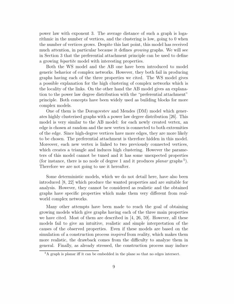
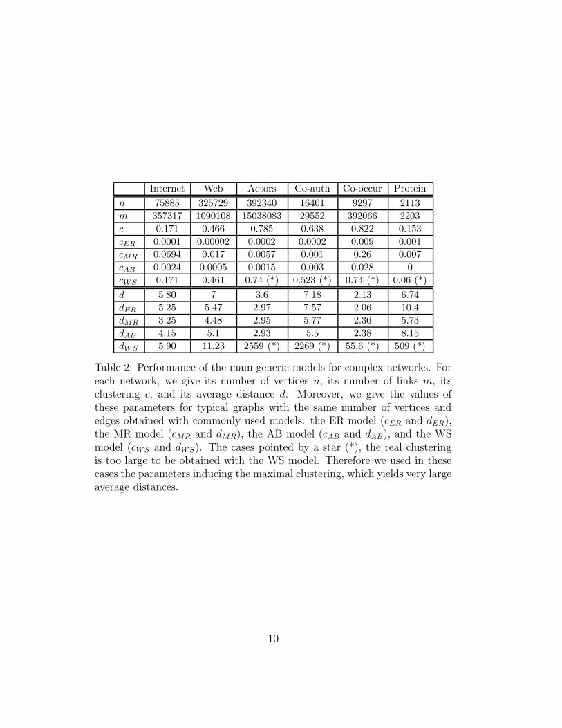
Table 2: Performance of the main generic models for complex networks. Foreach network, we give its number of vertices n, its number of links m, itsclustering c, and its average distance d. Moreover, we give the values ofthese parameters for typical graphs with the same number of vertices andedges obtained with commonly used models: the ER model (cER and dER),the MR model (cMR and dMR), the AB model (cAB and dAB), and the WSmodel (cWS and dWS). The cases pointed by a star (*), the real clusteringis too large to be obtained with the WS model. Therefore we used in thesecases the parameters inducing the maximal clustering, which yields very largeaverage distances.
10
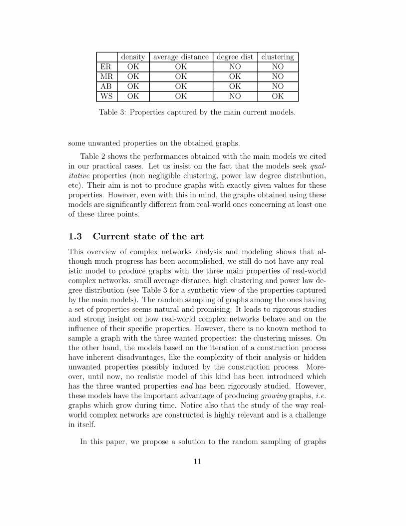
density average distance degree dist clusteringER OK OK NO NOMR OK OK OK NOAB OK OK OK NOWS OK OK NO OK
Table 3: Properties captured by the main current models.
some unwanted properties on the obtained graphs.
Table 2 shows the performances obtained with the main models we citedin our practical cases. Let us insist on the fact that the models seek qual-itative properties (non negligible clustering, power law degree distribution,etc). Their aim is not to produce graphs with exactly given values for theseproperties. However, even with this in mind, the graphs obtained using thesemodels are significantly different from real-world ones concerning at least oneof these three points.
1.3 Current state of the art
This overview of complex networks analysis and modeling shows that al-though much progress has been accomplished, we still do not have any real-istic model to produce graphs with the three main properties of real-worldcomplex networks: small average distance, high clustering and power law de-gree distribution (see Table 3 for a synthetic view of the properties capturedby the main models). The random sampling of graphs among the ones havinga set of properties seems natural and promising. It leads to rigorous studiesand strong insight on how real-world complex networks behave and on theinfluence of their specific properties. However, there is no known method tosample a graph with the three wanted properties: the clustering misses. Onthe other hand, the models based on the iteration of a construction processhave inherent disadvantages, like the complexity of their analysis or hiddenunwanted properties possibly induced by the construction process. More-over, until now, no realistic model of this kind has been introduced whichhas the three wanted properties and has been rigorously studied. However,these models have the important advantage of producing growing graphs, i.e.graphs which grow during time. Notice also that the study of the way real-world complex networks are constructed is highly relevant and is a challengein itself.
In this paper, we propose a solution to the random sampling of graphs
11
which have all the three wanted properties. To achieve this, we focus onanother property of all real-world complex networks, namely their underlyingbipartite structure (Section 2). We then propose two models: the randomsampling of bipartite graphs with prescribed degree distributions, and thegrowing bipartite model with preferential attachment (Section 3). Indeed, asshown in Sections 4 and 5, respectively formally and experimentally, thesemodels induce the three wanted properties. This means that they can beviewed as consequences of the underlying bipartite structure of all complexnetworks, which is our main contribution.
2 Complex networks as bipartite graphs
A bipartite graph is a triple G = (>,⊥, E) where > and ⊥ are two disjointsets of vertices, respectively the top and bottom vertices, and E ⊆ > × ⊥is the set of edges. The difference with classical graphs lies in the fact thatedges exist only between top vertices and bottom vertices.
Two degree distributions can naturally be associated to such a graph,namely the top degree distribution: >k = |{t∈>:d(t)=k}|
|>| and the bottom degree
distribution: ⊥k = |{t∈⊥:d(t)=k}||⊥| . These two distributions play a central role
in the following.
Natural bipartite structures
As already noticed for instance in [55, 34], some complex networks display anatural bipartite structure. Among our examples, one can view Actors (twoactors are linked if they are part of a same cast) as a bipartite graph where> is the set of movies, ⊥ is the set of actors, and each actor is linked to themovies he/she played in. Coauthoring can also be viewed this way with >being the set of papers and ⊥ being the set of authors, each author beinglinked to the papers he/she (co-)signed. Likewise, in Cooccurrence one canlink each sentence to the words it contains.
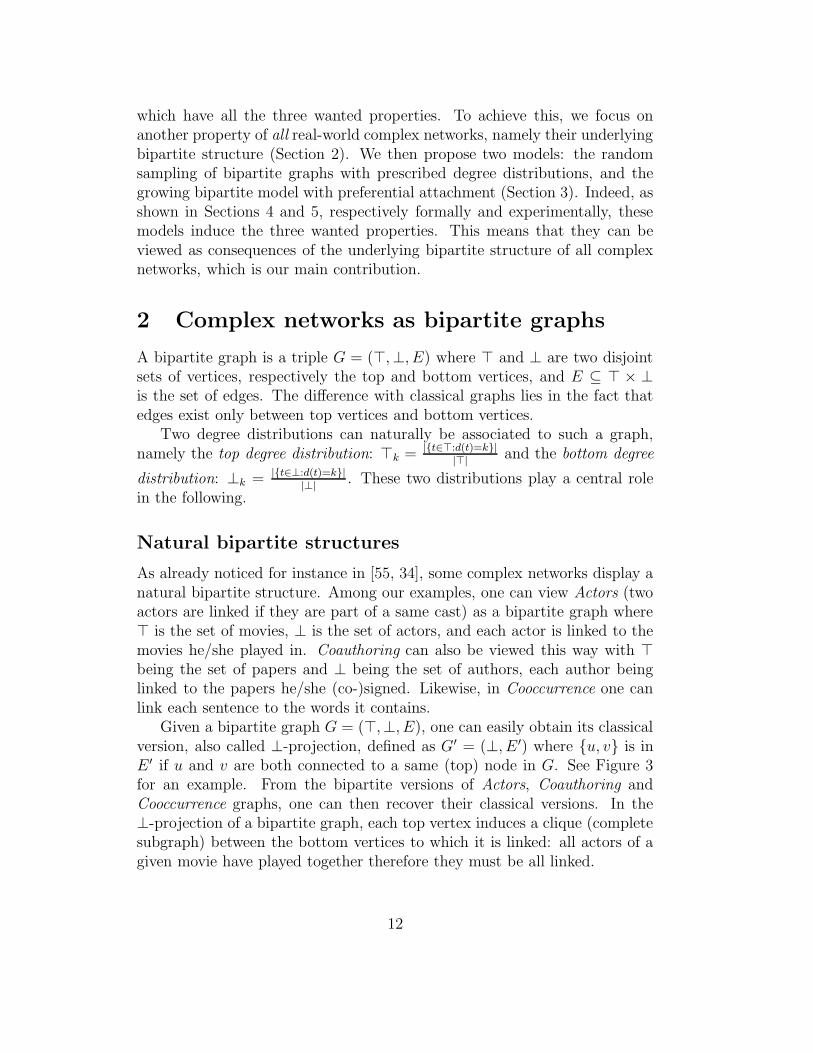
Given a bipartite graph G = (>,⊥, E), one can easily obtain its classicalversion, also called ⊥-projection, defined as G′ = (⊥, E ′) where {u, v} is inE ′ if u and v are both connected to a same (top) node in G. See Figure 3for an example. From the bipartite versions of Actors, Coauthoring andCooccurrence graphs, one can then recover their classical versions. In the⊥-projection of a bipartite graph, each top vertex induces a clique (completesubgraph) between the bottom vertices to which it is linked: all actors of agiven movie have played together therefore they must be all linked.
12
A B C D E F
A
B
E
D
C F
Figure 3: A bipartite network and its ⊥-projection. Notice that the link{B,C} is obtained twice since B and C have two neighbors in common inthe bipartite network.
However, given the ⊥-projection of a bipartite graph, it is in general notpossible to recover the bipartite graph from which it has been obtained in anunique way. Similarly if a graph is not naturally bipartite there may existmany bipartite versions of it.
Recovering a bipartite structure
For the sake of completeness, we now recall and detail the decompositionscheme we proposed in [34], which produces a bipartite graph from any givengraph, such that the latter is be the ⊥-projection of the obtained bipartitegraph. The aim of this scheme is that the obtained bipartite graph shouldhave properties similar to the ones met in natural bipartite graphs, namelythe number of top vertices has the same order of magnitude as the numberof bottom vertices and there are some high-degree top nodes (see below andFigure 7).
First notice that the decomposition scheme is nothing but a clique cov-ering problem: it computes a set of cliques (which will correspond to thetop nodes in the bipartite graph) such that each edge belongs to at least oneclique (which ensures that the ⊥-projection of the decomposition is exactlythe original graph). Simple ideas to cover the graph with cliques might be toconsider each edge as a clique, or to consider all maximal cliques. However,the first approach would not yield large cliques while the second one couldyield too many cliques (the number of maximal cliques may be exponential).
To reach our goal, we proposed [34] the following decomposition. We pickfor each edge a largest clique containing it: a clique whose size is maximalamong the ones containing the edge. Notice that this clique may contain onlytwo vertices. Moreover, if there are several such cliques for the same edge,we pick one at random. This decomposition ensures the complete covering ofthe graph. Moreover, the number of cliques is at most equal to the numberof edges, which is of the order of the number of vertices. Finally since wetake largest cliques, we expect to find most of the large cliques contained in
13
the graph.In the case of Figure 3 we obtain several cliques of size 2 (namely {C,E}
and {D,F}), and we have to choose at random between {A,B,C} and{B,C,D} when considering the edge {B,C}. However, these two cliquesare obtained from other edges, and we finally obtain a unique decompositionwhich is nothing but the bipartite graph on the left of the figure.
The central aim of our decomposition scheme is, given the ⊥-projectionof a natural bipartite graph, to produce an artificial bipartite graph similarto the original bipartite graph itself. A way to evaluate it is therefore todecompose the ⊥-projection version of a natural bipartite complex networkand to compare the obtained bipartite network to the original one. This iswhat we do in Figure 4.
Actors
Extracted
Original
1
10
100
1000
10000
1 10 100
Cooccurence
Original
Extracted
1
10
100
1000
1 10 100 1000
Original
Extracted
Coauthoring
0
1000
2000
3000
4000
5000
6000
7000
8000
9000
1 2 3 4 5 6 7 8
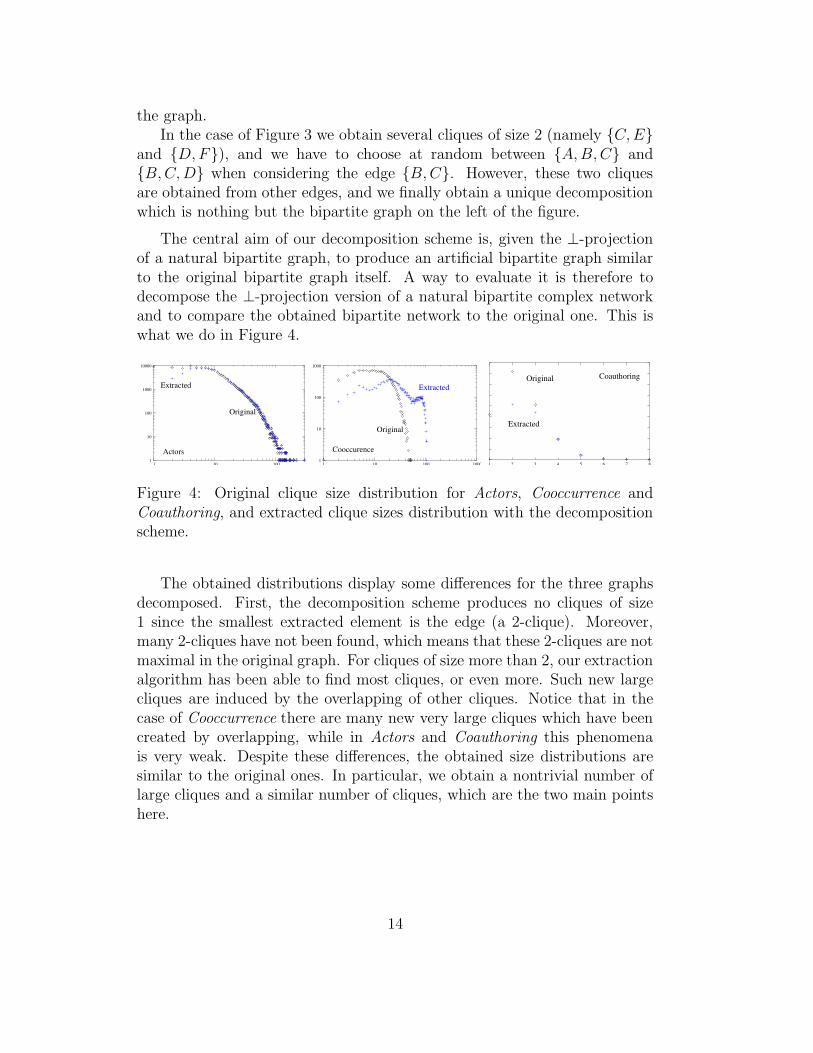
Figure 4: Original clique size distribution for Actors, Cooccurrence andCoauthoring, and extracted clique sizes distribution with the decompositionscheme.
The obtained distributions display some differences for the three graphsdecomposed. First, the decomposition scheme produces no cliques of size1 since the smallest extracted element is the edge (a 2-clique). Moreover,many 2-cliques have not been found, which means that these 2-cliques are notmaximal in the original graph. For cliques of size more than 2, our extractionalgorithm has been able to find most cliques, or even more. Such new largecliques are induced by the overlapping of other cliques. Notice that in thecase of Cooccurrence there are many new very large cliques which have beencreated by overlapping, while in Actors and Coauthoring this phenomenais very weak. Despite these differences, the obtained size distributions aresimilar to the original ones. In particular, we obtain a nontrivial number oflarge cliques and a similar number of cliques, which are the two main pointshere.
14
Practical computation
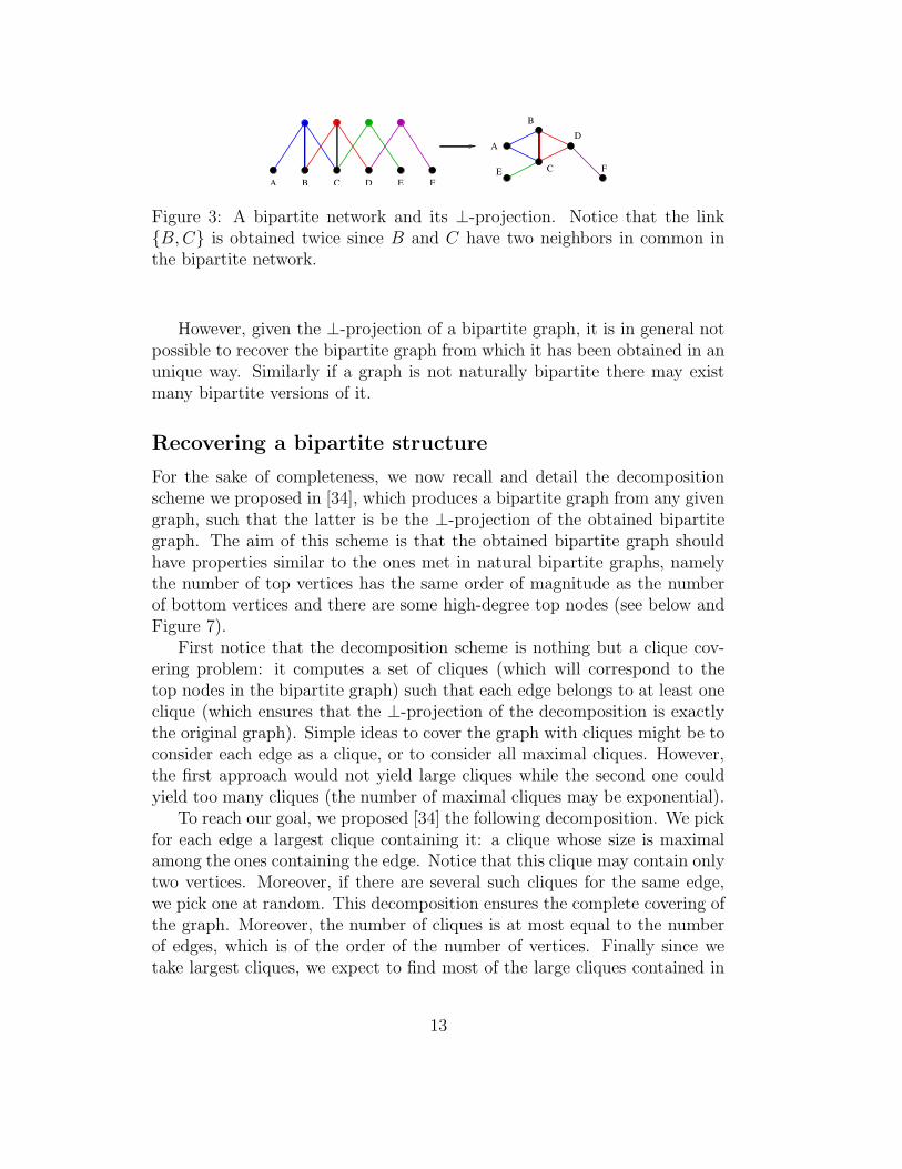
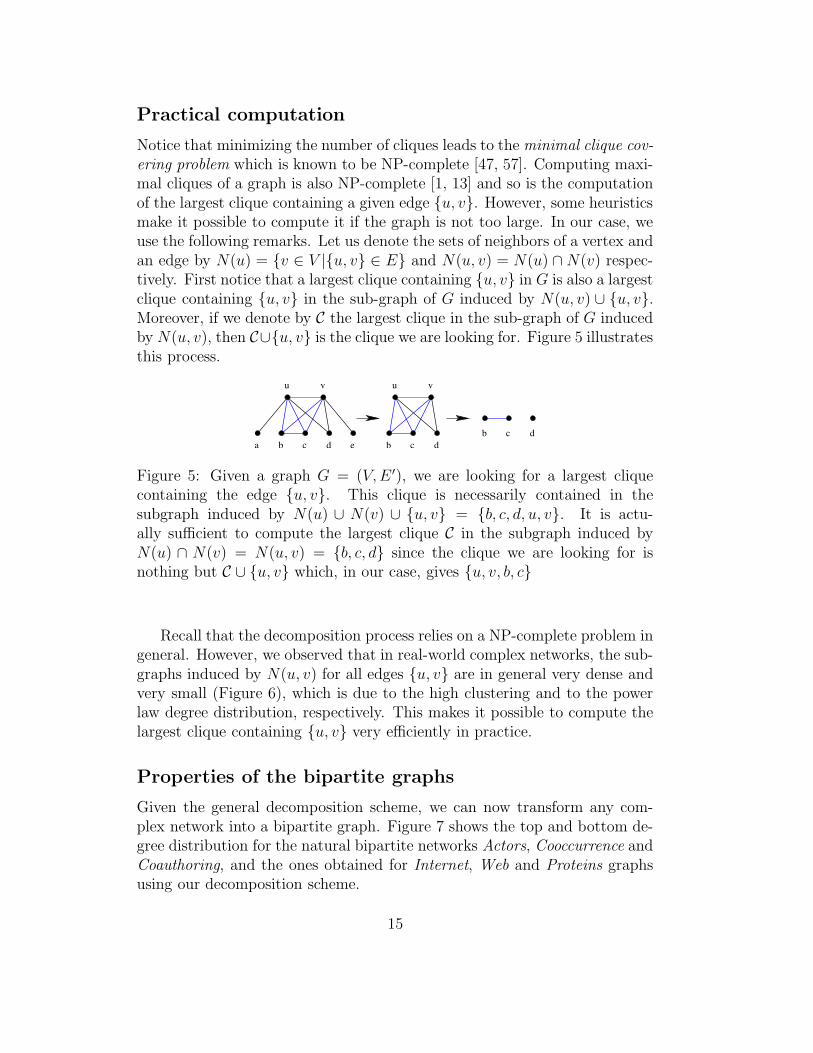
Notice that minimizing the number of cliques leads to the minimal clique cov-ering problem which is known to be NP-complete [47, 57]. Computing maxi-mal cliques of a graph is also NP-complete [1, 13] and so is the computationof the largest clique containing a given edge {u, v}. However, some heuristicsmake it possible to compute it if the graph is not too large. In our case, weuse the following remarks. Let us denote the sets of neighbors of a vertex andan edge by N(u) = {v ∈ V |{u, v} ∈ E} and N(u, v) = N(u) ∩ N(v) respec-tively. First notice that a largest clique containing {u, v} in G is also a largestclique containing {u, v} in the sub-graph of G induced by N(u, v) ∪ {u, v}.Moreover, if we denote by C the largest clique in the sub-graph of G inducedby N(u, v), then C∪{u, v} is the clique we are looking for. Figure 5 illustratesthis process.
u v u v
a b c d e b c db c d
Figure 5: Given a graph G = (V,E ′), we are looking for a largest cliquecontaining the edge {u, v}. This clique is necessarily contained in thesubgraph induced by N(u) ∪ N(v) ∪ {u, v} = {b, c, d, u, v}. It is actu-ally sufficient to compute the largest clique C in the subgraph induced byN(u) ∩ N(v) = N(u, v) = {b, c, d} since the clique we are looking for isnothing but C ∪ {u, v} which, in our case, gives {u, v, b, c}
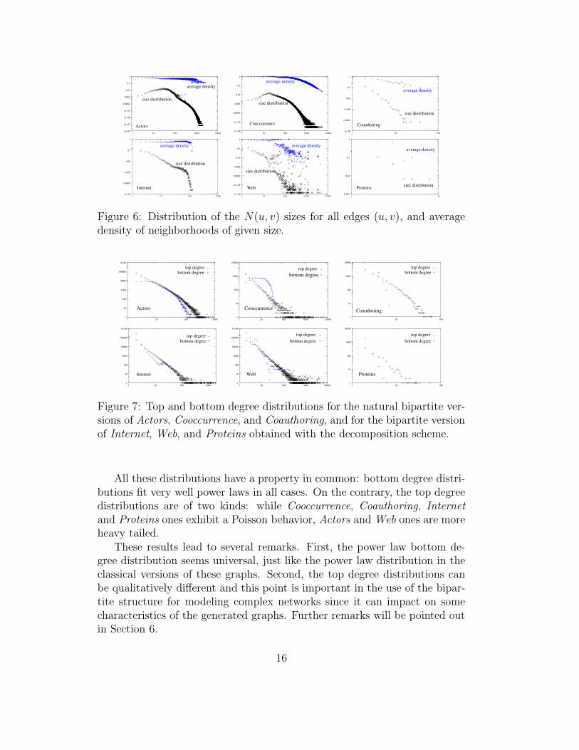
Recall that the decomposition process relies on a NP-complete problem ingeneral. However, we observed that in real-world complex networks, the sub-graphs induced by N(u, v) for all edges {u, v} are in general very dense andvery small (Figure 6), which is due to the high clustering and to the powerlaw degree distribution, respectively. This makes it possible to compute thelargest clique containing {u, v} very efficiently in practice.
Properties of the bipartite graphs
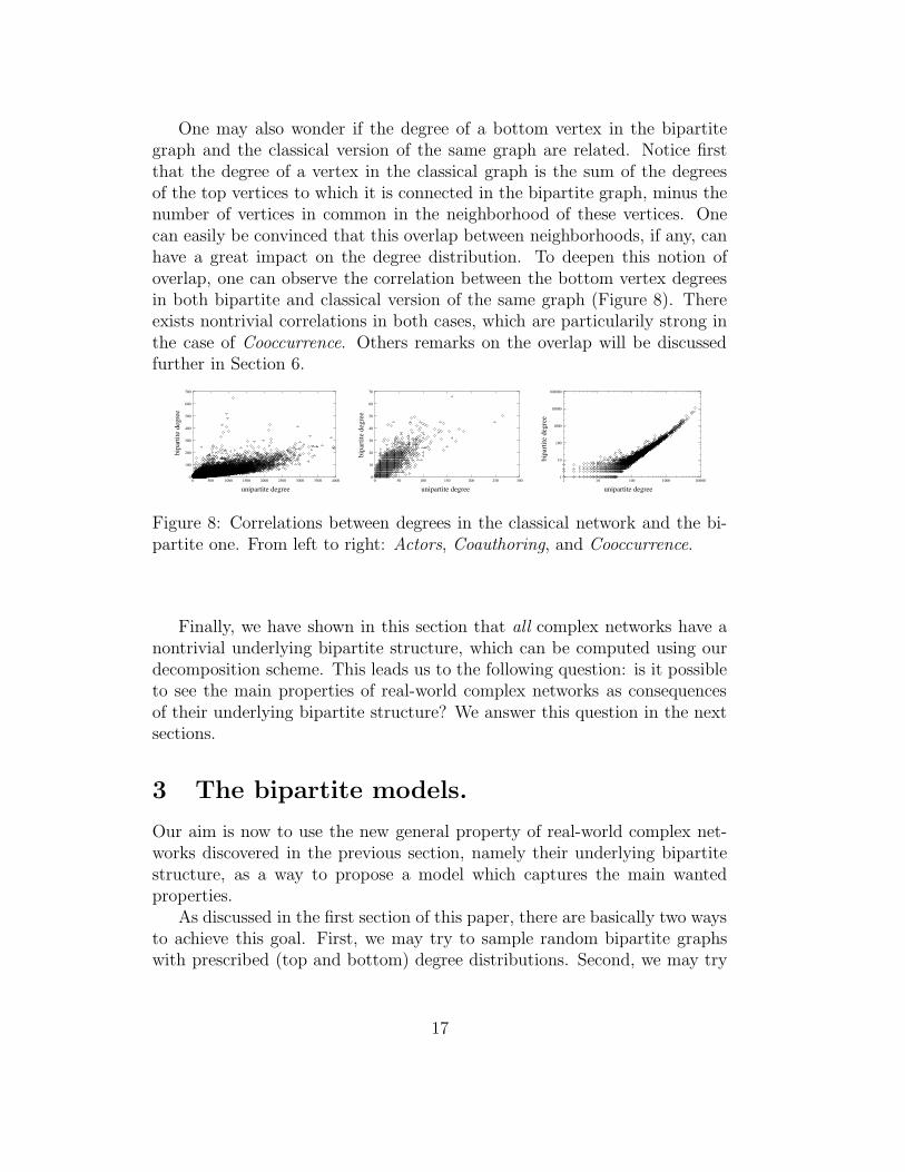
Given the general decomposition scheme, we can now transform any com-plex network into a bipartite graph. Figure 7 shows the top and bottom de-gree distribution for the natural bipartite networks Actors, Cooccurrence andCoauthoring, and the ones obtained for Internet, Web and Proteins graphsusing our decomposition scheme.
15
Actors
average density
size distribution
1e−08
1e−07
1e−06
1e−05
0.0001
0.001
0.01
0.1
1
1 10 100 1000 10000
Cooccurrence
size distribution
average density
1e−06
1e−05
0.0001
0.001
0.01
0.1
1
1 10 100 1000 10000
Coauthoring
average density
size distribution
1e−05
0.0001
0.001
0.01
0.1
1
1 10 100
Internet
average density
size distribution
1e−05
0.0001
0.001
0.01
0.1
1
1 10 100 1000
average density
size distribution
Web 1e−06
1e−05
0.0001
0.001
0.01
0.1
1
1 10 100 1000 10000
Proteins size distribution
average density
0.001
0.01
0.1
1
1 10
Figure 6: Distribution of the N(u, v) sizes for all edges (u, v), and averagedensity of neighborhoods of given size.
bottom degreetop degree
Actors
1
10
100
1000
10000
100000
1e+06
1 10 100 1000
top degree
Cooccurrence
bottom degree
1
10
100
1000
10000
1 10 100 1000 10000
top degreebottom degree
Coauthoring1
10
100
1000
10000
1 10 100
Internet
top degreebottom degree
1
10
100
1000
10000
100000
1e+06
1 10 100 1000
Web
top degreebottom degree
1
10
100
1000
10000
100000
1e+06
1 10 100 1000 10000
top degreebottom degree
Proteins
1
10
100
1000
10000
1 10 100
Figure 7: Top and bottom degree distributions for the natural bipartite ver-sions of Actors, Cooccurrence, and Coauthoring, and for the bipartite versionof Internet, Web, and Proteins obtained with the decomposition scheme.
All these distributions have a property in common: bottom degree distri-butions fit very well power laws in all cases. On the contrary, the top degreedistributions are of two kinds: while Cooccurrence, Coauthoring, Internetand Proteins ones exhibit a Poisson behavior, Actors and Web ones are moreheavy tailed.
These results lead to several remarks. First, the power law bottom de-gree distribution seems universal, just like the power law distribution in theclassical versions of these graphs. Second, the top degree distributions canbe qualitatively different and this point is important in the use of the bipar-tite structure for modeling complex networks since it can impact on somecharacteristics of the generated graphs. Further remarks will be pointed outin Section 6.
16
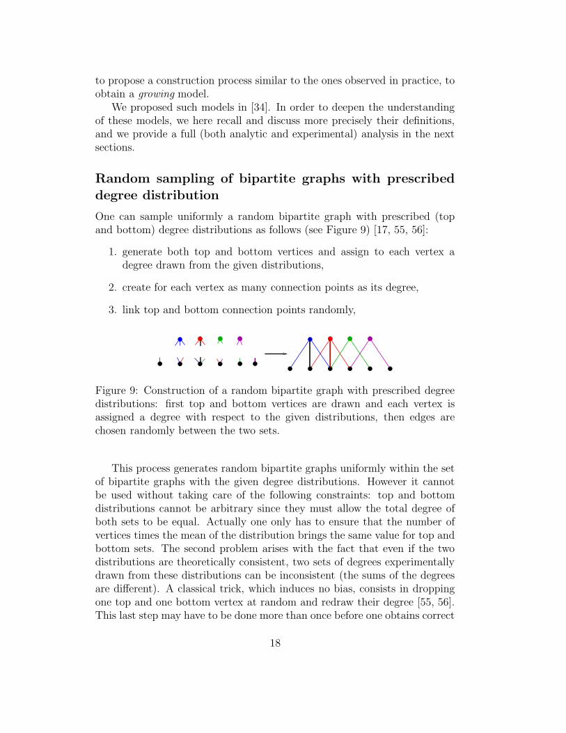
One may also wonder if the degree of a bottom vertex in the bipartitegraph and the classical version of the same graph are related. Notice firstthat the degree of a vertex in the classical graph is the sum of the degreesof the top vertices to which it is connected in the bipartite graph, minus thenumber of vertices in common in the neighborhood of these vertices. Onecan easily be convinced that this overlap between neighborhoods, if any, canhave a great impact on the degree distribution. To deepen this notion ofoverlap, one can observe the correlation between the bottom vertex degreesin both bipartite and classical version of the same graph (Figure 8). Thereexists nontrivial correlations in both cases, which are particularily strong inthe case of Cooccurrence. Others remarks on the overlap will be discussedfurther in Section 6.
bipa
rtite
deg
ree
unipartite degree
0
100
200
300
400
500
600
700
0 500 1000 1500 2000 2500 3000 3500 4000
bipa
rtite
deg
ree
unipartite degree
0
10
20
30
40
50
60
70
0 50 100 150 200 250 300
bipa
rtite
deg
ree
unipartite degree
1
10
100
1000
10000
100000
1 10 100 1000 10000
Figure 8: Correlations between degrees in the classical network and the bi-partite one. From left to right: Actors, Coauthoring, and Cooccurrence.
Finally, we have shown in this section that all complex networks have anontrivial underlying bipartite structure, which can be computed using ourdecomposition scheme. This leads us to the following question: is it possibleto see the main properties of real-world complex networks as consequencesof their underlying bipartite structure? We answer this question in the nextsections.
3 The bipartite models.
Our aim is now to use the new general property of real-world complex net-works discovered in the previous section, namely their underlying bipartitestructure, as a way to propose a model which captures the main wantedproperties.
As discussed in the first section of this paper, there are basically two waysto achieve this goal. First, we may try to sample random bipartite graphswith prescribed (top and bottom) degree distributions. Second, we may try
17
to propose a construction process similar to the ones observed in practice, toobtain a growing model.
We proposed such models in [34]. In order to deepen the understandingof these models, we here recall and discuss more precisely their definitions,and we provide a full (both analytic and experimental) analysis in the nextsections.
Random sampling of bipartite graphs with prescribed
degree distribution
One can sample uniformly a random bipartite graph with prescribed (topand bottom) degree distributions as follows (see Figure 9) [17, 55, 56]:
1. generate both top and bottom vertices and assign to each vertex adegree drawn from the given distributions,
2. create for each vertex as many connection points as its degree,
3. link top and bottom connection points randomly,
Figure 9: Construction of a random bipartite graph with prescribed degreedistributions: first top and bottom vertices are drawn and each vertex isassigned a degree with respect to the given distributions, then edges arechosen randomly between the two sets.
This process generates random bipartite graphs uniformly within the setof bipartite graphs with the given degree distributions. However it cannotbe used without taking care of the following constraints: top and bottomdistributions cannot be arbitrary since they must allow the total degree ofboth sets to be equal. Actually one only has to ensure that the number ofvertices times the mean of the distribution brings the same value for top andbottom sets. The second problem arises with the fact that even if the twodistributions are theoretically consistent, two sets of degrees experimentallydrawn from these distributions can be inconsistent (the sums of the degreesare different). A classical trick, which induces no bias, consists in droppingone top and one bottom vertex at random and redraw their degree [55, 56].This last step may have to be done more than once before one obtains correct
18
values but finally the implementation and use of the model is very simpleand efficient [17].
Note that, just like with the MR model, multiple edges may appear.Again, one can easily show that they can be neglected when the graph islarge. Moreover, some approaches exist [38, 44] which can easily be modifiedto obtain random bipartite graphs without multiples edges. This is howeverout of the scope of this paper.
Growing bipartite model with preferential attachment
The random bipartite model assumes that two distributions, for both topand bottom degrees, are explicitly given. One can also use other rules (pref-erential attachment for instance) to define them implicitly and introduce agrowing model. Indeed, as already noticed, the bottom degree distributionsfollow a power law. This leads to the following model: at each step, a newtop vertex is added and its degree d is sampled from a prescribed (top) dis-tribution (which qualitatively varies between graphs). Then, for each of thed edges of the new vertex, either a new bottom vertex is added (with prob-ability 1− λ) or one is picked among the preexisting ones using preferentialattachment (with probability λ). The parameter λ is the overlap ratio, de-fined as the average ratio of preexisting bottom vertices to which a new topvertex is connected.
It is generally not possible to know exactly the order in which cliques arecreated on real-world bipartite graphs, but the average ratio can be computedglobally as λ = 1 − |⊥|P
d>. One can compute it and get 0.733 for Actors,
0.877 for Coauthoring and 0.949 for Cooccurrence. Notice that 1− λ can berewritten and is simply the inverse average bottom degree (since
∑d> =∑
d⊥), therefore a high overlap ratio yields a high average bottom degree(since only few nodes are created at each time step).
At each step of the construction process, the bipartite graph has therequired degree distributions: the prescribed top degree distribution is ob-tained by construction while the power law degree distribution is obtainedusing preferential attachment, which can be shown formally in exactly thesame way as in the original AB model [3]. Notice moreover that this con-struction process is very similar to the one observed in some real-world cases.For instance, Actors is built exactly this way: when a new movie is produced(which corresponds to the addition of a top vertex), it is linked to actorsaccording to their popularity, and to some new actors, playing in a movie forthe first time.
19
Bipartite models and classical graphs
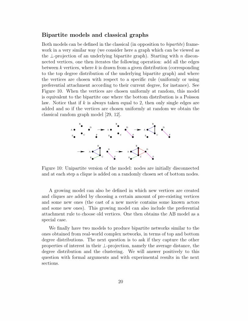
Both models can be defined in the classical (in opposition to bipartite) frame-work in a very similar way (we consider here a graph which can be viewed asthe ⊥-projection of an underlying bipartite graph). Starting with n discon-nected vertices, one then iterates the following operation: add all the edgesbetween k vertices, where k is drawn from a given distribution (correspondingto the top degree distribution of the underlying bipartite graph) and wherethe vertices are chosen with respect to a specific rule (uniformly or usingpreferential attachment according to their current degree, for instance). SeeFigure 10. When the vertices are chosen uniformly at random, this modelis equivalent to the bipartite one where the bottom distribution is a Poissonlaw. Notice that if k is always taken equal to 2, then only single edges areadded and so if the vertices are chosen uniformly at random we obtain theclassical random graph model [29, 12].
A
B
E
D
C F
A
B
E
D
C F
A
B
E
D
C F
A
B
E
D
C F
A
B
E
D
C F
Figure 10: Unipartite version of the model: nodes are initially disconnectedand at each step a clique is added on a randomly chosen set of bottom nodes.
A growing model can also be defined in which new vertices are createdand cliques are added by choosing a certain amount of pre-existing verticesand some new ones (the cast of a new movie contains some known actorsand some new ones). This growing model can also include the preferentialattachment rule to choose old vertices. One then obtains the AB model as aspecial case.
We finally have two models to produce bipartite networks similar to theones obtained from real-world complex networks, in terms of top and bottomdegree distributions. The next question is to ask if they capture the otherproperties of interest in their ⊥-projection, namely the average distance, thedegree distribution and the clustering. We will answer positively to thisquestion with formal arguments and with experimental results in the nextsections.
20
4 Analysis of the models.
Our aim in this section is to give formal proofs for the main properties ofthe ⊥-projection of a random bipartite graph with prescribed degree distribu-tions. Some of these properties, and others, have been studied independentlyin [55, 56] with different techniques and a different point of view. We how-ever believe that our proofs give new insight on these properties, thereforewe give them below. In particular, our proof techniques may be consideredas more mathematically rigorous.
Since these properties are induced by a typical graph (this is what ran-dom sampling gives us), this is a way to answer the following question: whatproperties are induced by the underlying bipartite structure? In particu-lar, can we see the main properties of real-world complex networks, namelylow average distance, power law degree distribution and high clustering, asconsequences of the underlying bipartite structure?
We will see that it is indeed the case. Notice that many other properties,like the size distribution of the connected components for instance, are ofhigh interest. It is shown in [55] that under reasonable conditions on thedegree distributions the ⊥-projection is connected, or at least has a giantcomponent. In all the practical cases, these conditions are fulfilled, thereforewe will restrict ourselves to this case.
Degree distribution
Let us first consider the degree distribution of the ⊥-projection of a randombipartite graph G = (>,⊥, E). Given a bottom vertex u, we denote byd(u) the degree of u in the bipartite graph, and by dU(u) its degree in its⊥-projection. We want to study the distribution of dU(u) (we actually dealhere with the expected value for a randomly chosen u).
Lemma 1 Let us consider a bottom vertex u ∈ ⊥. The expected number ofbottom vertices which have a neighbor (in >) in common with u, i.e. dU(u),is:
d(u)
|>| ·∑
t6=ud(t) +O
(d(u)2
|>|2 ·∑
t6=ud(t)2
)
Proof. The exact expected value of dU(u) is given by:
dU(u) =∑
t6=u
(1−
(|>|−d(u)d(t)
)( |>|d(t)
))
21
since the probability that a given bottom vertex t has a top neighbor incommon with u depends only on the degree of both vertices and the num-ber of top vertices. To simplify this formula, we can approximate the ratio(|>|−d(u)
d(t)
)/( |>|d(t)
)as follows:
(|>|−d(u)d(t)
)( |>|d(t)
) =(|>| − d(u))!(|>| − d(t))!
|>|!(|>| − d(u)− d(t))!
∼ (|>| − d(t))d(u)
|>|d(u)
∼ 1− d(t)d(u)
|>| +O((
d(t)d(u)
|>|
)2)
Therefore:
d>(u) ∼∑
t6=u
(d(t)d(u)
|>| +O((
d(t)d(u)
|>|
)2))
∼ d(u)
|>|∑
t6=ud(t) +O
(d(u)2
|>|2∑
t6=ud(t)2
)
which is the formula of the claim. �
This lemma makes it possible to compute the probability for a vertexu in the ⊥-projection graph to have a given degree k if the bottom degreedistribution is a power law with exponent β:
P [dU(u) = k] ∼ P [d(u) =n∑
t6=u d(t)· k]
∼ 1
(∑
t6=u d(t)) · k)β∼ k−β
Therefore, as long as the bottom degree distribution follows a power law,the degree distribution in the ⊥-projection of the graph also follows a powerlaw with the same exponent, which is indeed the case in practice as one cancheck in Figures 11 and 7.
22
Average distance
To study the average distance in the ⊥-projection of a graph obtained withthe model, we will use a result from L. Lu about the diameter (i.e. the largestdistance between any two vertices) of some specific random graphs:
Theorem 1 [39] Let G = (V,E) be a graph whose vertices are weightedwith weights w1, · · · , wn, such that each edge {i, j} appears with probabilitywi · wj · p. If the degrees of the vertices in V follow a power law with anexponent β strictly greater than 2, then the diameter of the graph G is almostsurely Θ(log(n))6.
This theorem, together with the one presented above on the degree dis-tribution of the ⊥-projection of the graph, leads to the following result:
Theorem 2 Let G = (>,⊥, E) be a bipartite graph such that the bottomdegree distribution follows a power law with an exponent greater than 2. Thenthe diameter of the ⊥-projection of G is almost surely Θ(log(|⊥|)).
Proof. Given two bottom vertices u and v in⊥, the probability that they areconnected in the ⊥-projection is equal to the probability that they are bothlinked to a same top vertex in G. This probability is exactly proportional tod⊥(u) ·d⊥(v). Therefore we can apply Theorem 1 considering that the weightof each vertex is its degree and so the connection probability is ensured, andas long as bottom degree distribution follows a power law with an exponentβ strictly greater than 2. The diameter of the ⊥-projection of the graphtherefore is almost surely Θ(log(|⊥|)). �
Since the diameter is an upper bound for the average distance, this the-orem implies that the average distance of the ⊥-projection scales at most asfast as the logarithm of its number of nodes. Notice that, as in the case ofrandom networks [12, 18, 21, 28, 39, 55, 56], the average distance may groweven slower.
Clustering
Recall that the clustering of a vertex v of degree at least 2 in a graph is theprobability that two of its neighbors are linked [64], i.e. the number of trian-gles to which v belongs over the number of connected triples centered on it:c(v) = |4(v)|
|∧(v)| . Then the clustering of the graph is defined as: 1N
∑v,d(v)>1 c(v).
6One denotes by f = Θ(g) the fact that f = O(g) and g = O(f)i.
23
We define the clustering of a vertex restricted to a part of its neighborhoodas its clustering in the subgraph induced by this part of its neighborhood.
Hereafter we give a lower bound for the clustering of a graph G′ whichis the ⊥-projection of a bipartite graph G = (>,⊥, E) obtained using therandom bipartite model. We show that, under reasonable assumptions on thetop and bottom degree distributions, it is bounded by a value independentof the size of the graph. This shows that the model produces graphs withnontrivial clustering.
Before entering in the core of this section, notice that an approximationformula for the clustering of such a graph is given in [55, 56]. Here we givean exact formula for a lower bound. Both are interesting since the first onegives an expected value which is indeed very close to the real value, while thesecond one gives a guaranty that the exact value is above the given quantity.We used this approach because we seek qualitative results only, and so it issufficient for us to show that the clustering does not tend to 0 when the sizeof the graph grows. The lower bound achieves this goal.
First notice that the probability for two top vertices to have more thanjust one bottom vertex in common in their neighborhood tends to zero whenthe size of the graph grows. We therefore consider any vertex b in the ⊥-projection of the graph and we suppose that its neighborhood is composedof a set of disjoint cliques. We will prove the following:
• the effect of the number of top vertices of degree 2 to which b is con-nected on its clustering is negligible, and
• the clustering of b can be bounded by a value which depends only onits degree.
Lemma 2 Let >>2 denote the set of top neighbors of b in G with degreestrictly greater than 2, and ⊥>2 denote the set of bottom neighbors of >>2.Let p be the fraction of neighbors of b which belong to ⊥>2, and α be theclustering of b (in G′) restricted to ⊥>2.
Then the clustering of b in G′ scales as p2 · α.
Proof. The fact that the clustering of b restricted to ⊥>2 is α implies that|4⊥>2(b)| = α ·
(p·d2
). If we consider the whole neighborhood of b, instead
of just ⊥>2, the number of triangles does not change while the number ofconnected triples increases:
24
c(b) =α ·(p·d2
)(d2
)
= α · p · d((p · d− 1)
d(d− 1)
∼ p2 · α
which is the formula of the claim. �
Therefore, as long as p is a constant, one can neglect the top vertices ofdegree 2 when computing the clustering of a given vertex. Now let us provethat the clustering of a bottom vertex can be related to its degree.
Lemma 3 If b is connected only to top vertices of degree at least 3 in G,then:
c(b) ≥ 1
2 · d(b)− 1
Proof. Suppose b is connected to two top vertices, t1 and t2, of degree atleast 3 (we deal with the general case below). Then the clustering of b is:
c(b) =
(d(t1)−1
2
)+(d(t2)−1
2
)(d(t1)+d(t2)−2
2
)
Suppose now that b is connected to t2 and t′1 such that d(t′1) = d(t1) + 1,then the clustering of b is:
c′(b) =
(d(t1)+1−1
2
)+(d(t2)−1
2
)(d(t1)+d(t2)−1
2
)
and:
c′(b)− c(b) =2 · (d(t2)− 1)
(d(t1) + d(t2)− 2) · (d(t1) + d(t2)− 3)
> 0
which means that the clustering grows with the degree of t1 and t2. A lowerbound for the clustering of b can therefore be obtained when both t1 and t2have the smallest possible degree, 3.
This can be extended to the case where b has more than two top neighborsto obtain the following lower bound:
25
c(b) =
∑ti
(d(ti)−1
2
)(P
ti(d(ti)−1)
2
)
≥∑
ti
(3−1
2
)(P
ti(3−1)
2
) ≥ 1
2 · d(b)− 1
which is the formula of the claim. �
The clustering of the classical graph G′ can now be easily approximated:
c(G′) ∼ 1
N
∑
b∈⊥
1
2d(b)− 1
As long as there is a linear number c · N of vertices b of degree 2, thesum scales linearly with N :
∑b∈⊥
12·d(b)−1
≥∑b,d(b)=2
(1
2·2−1
)= c·N
3(we could
have considered vertices of any constant degree k instead of 2). Therefore thelower bound for the clustering is independent of N . This holds in particularfor power law networks since the number of vertices of degree 2 is of the orderof N · 2−α.
Since we do not consider top vertices of degree 2 in the last formula (dueto Lemma 2), we must also ensure that the number of such top neighborsrepresent at most a constant fraction (not tending to 1) of the neighbors.This is indeed the case for most distributions and in particular for the onesmet in practice. We finally obtain that the clustering of the graph is largerthan a non-zero constant independently of the size of the graph, which wasour aim.
5 Experimental results
The formal results of the previous section give a precise intuition on how therandom bipartite graph model with prescribed degree distributions behaves.We can also check its properties experimentally by generating graphs usingthis model and the same parameters as the ones measured on real-worldcomplex networks. This is what we do in this section with our six examples,for the purely random bipartite model as well as for the one with preferentialattachment.
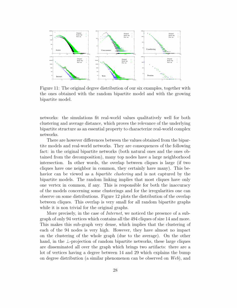
Table 4 and 5 give the values obtained for the average distance and theclustering. Figure 11 shows a comparison between the degree distributionsof the original graphs, and the ones obtained with the two bipartite models.
26
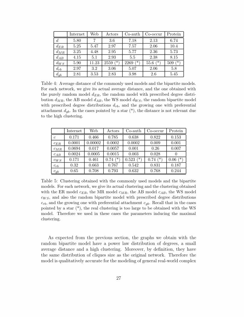
Internet Web Actors Co-auth Co-occur Protein
d 5.80 7 3.6 7.18 2.13 6.74
dER 5.25 5.47 2.97 7.57 2.06 10.4
dMR 3.25 4.48 2.95 5.77 2.36 5.73
dAB 4.15 5.1 2.93 5.5 2.38 8.15
dWS 5.90 11.23 2559 (*) 2269 (*) 55.6 (*) 509 (*)
drb 2.97 3.2 3.06 5.07 2.06 5.8
dgb 2.81 3.53 2.83 3.98 2.6 5.45
Table 4: Average distance of the commonly used models and the bipartite models.For each network, we give its actual average distance, and the one obtained withthe purely random model dER, the random model with prescribed degree distri-bution dMR, the AB model dAB , the WS model dWS , the random bipartite modelwith prescribed degree distributions drb, and the growing one with preferentialattachment dgb. In the cases pointed by a star (*), the distance is not relevant dueto the high clustering.
Internet Web Actors Co-auth Co-occur Protein
c 0.171 0.466 0.785 0.638 0.822 0.153
cER 0.0001 0.00002 0.0002 0.0002 0.009 0.001
cMR 0.0694 0.017 0.0057 0.001 0.26 0.007
cAB 0.0024 0.0005 0.0015 0.003 0.028 0
cWS 0.171 0.461 0.74 (*) 0.523 (*) 0.74 (*) 0.06 (*)
crb 0.32 0.663 0.767 0.542 0.831 0.187
cgb 0.65 0.708 0.793 0.632 0.768 0.244
Table 5: Clustering obtained with the commonly used models and the bipartitemodels. For each network, we give its actual clustering and the clustering obtainedwith the ER model cER, the MR model cMR, the AB model cAB , the WS modelcWS , and also the random bipartite model with prescribed degree distributionscrb, and the growing one with preferential attachment cgb. Recall that in the casespointed by a star (*), the real clustering is too large to be obtained with the WSmodel. Therefore we used in these cases the parameters inducing the maximalclustering.
As expected from the previous section, the graphs we obtain with therandom bipartite model have a power law distribution of degrees, a smallaverage distance and a high clustering. Moreover, by definition, they havethe same distribution of cliques size as the original network. Therefore themodel is qualitatively accurate for the modeling of general real-world complex
27
OriginalRand. bip.Pref. att.
Actors
1
10
100
1000
10000
100000
1 10 100 1000 10000 100000
OriginalRand. bip.Pref. att.
Cooccurence
1
10
100
1000
1 10 100 1000 10000
Rand. bip.Pref. att.
Coauthoring
Original
1
10
100
1000
10000
1 10 100 1000
Internet
OriginalRand. bip.Pref. att.
1
10
100
1000
10000
100000
1e+06
1 10 100 1000 10000
Web
OriginalRand. bip.Pref. att.
1
10
100
1000
10000
100000
1e+06
1 10 100 1000 10000 100000
Proteins
OriginalRand. bip.Pref. att.
1
10
100
1000
10000
1 10 100
Figure 11: The original degree distribution of our six examples, together withthe ones obtained with the random bipartite model and with the growingbipartite model.
networks: the simulations fit real-world values qualitatively well for bothclustering and average distance, which proves the relevance of the underlyingbipartite structure as an essential property to characterize real-world complexnetworks.
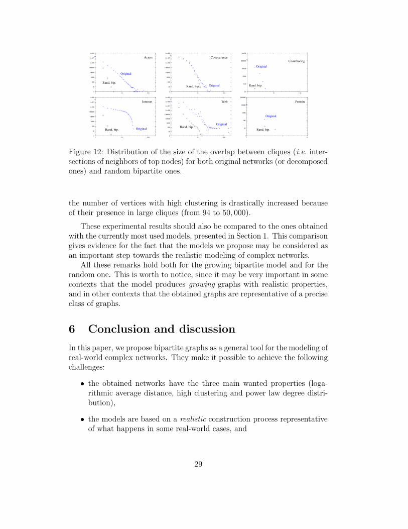
There are however differences between the values obtained from the bipar-tite models and real-world networks. They are consequences of the followingfact: in the original bipartite networks (both natural ones and the ones ob-tained from the decomposition), many top nodes have a large neighborhoodintersection. In other words, the overlap between cliques is large (if twocliques have one neighbor in common, they certainly have many). This be-havior can be viewed as a bipartite clustering and is not captured by thebipartite models. The random linking implies that most cliques have onlyone vertex in common, if any. This is responsible for both the inaccuracyof the models concerning some clusterings and for the irregularities one canobserve on some distributions. Figure 12 plots the distribution of the overlapbetween cliques. This overlap is very small for all random bipartite graphswhile it is non trivial for the original graphs.
More precisely, in the case of Internet, we noticed the presence of a sub-graph of only 94 vertices which contains all the 494 cliques of size 14 and more.This makes this sub-graph very dense, which implies that the clustering ofeach of the 94 nodes is very high. However, they have almost no impacton the clustering of the whole graph (due to the average). On the otherhand, in the ⊥-projection of random bipartite networks, these large cliquesare disseminated all over the graph which brings two artifacts: there are alot of vertices having a degree between 14 and 29 which explains the bumpon degree distribution (a similar phenomenon can be observed on Web), and
28
Original
Actors
Rand. bip.
1
10
100
1000
10000
100000
1e+06
1e+07
1e+08
1 10 100
OriginalRand. bip.
Cooccurence
1
10
100
1000
10000
100000
1e+06
1e+07
1e+08
1 10 100
Rand. bip.
Coauthoring
Original
10
100
1000
10000
100000
1e+06
1 10 100
Rand. bip. Original
Internet
1
10
100
1000
10000
100000
1e+06
1e+07
1e+08
1 10 100
Rand. bip.Original
Web
1
10
100
1000
10000
100000
1e+06
1e+07
1e+08
1e+09
1 10 100
Rand. bip.
Original
Protein
1
10
100
1000
10000
100000
1 10
Figure 12: Distribution of the size of the overlap between cliques (i.e. inter-sections of neighbors of top nodes) for both original networks (or decomposedones) and random bipartite ones.
the number of vertices with high clustering is drastically increased becauseof their presence in large cliques (from 94 to 50, 000).
These experimental results should also be compared to the ones obtainedwith the currently most used models, presented in Section 1. This comparisongives evidence for the fact that the models we propose may be considered asan important step towards the realistic modeling of complex networks.
All these remarks hold both for the growing bipartite model and for therandom one. This is worth to notice, since it may be very important in somecontexts that the model produces growing graphs with realistic properties,and in other contexts that the obtained graphs are representative of a preciseclass of graphs.
6 Conclusion and discussion
In this paper, we propose bipartite graphs as a general tool for the modeling ofreal-world complex networks. They make it possible to achieve the followingchallenges:
• the obtained networks have the three main wanted properties (loga-rithmic average distance, high clustering and power law degree distri-bution),
• the models are based on a realistic construction process representativeof what happens in some real-world cases, and
29
• their definitions are simple enough to make it possible to give someintuition and some proofs of their properties.
Moreover, they can be derived in two versions: one which relies on randomsampling among a class of graphs, and one which relies on an iterative con-struction process. This makes them suitable for a wide variety of usages.
Whereas many models have already been introduced, this one is the firstwhich reaches all these goals at the same time. In this sense, it may beconsidered as a significant step towards the realistic modeling of complexnetworks. Moreover, it is very simple to obtain graphs using this model (weprovide a generator at [17]), which makes it highly suitable for simulationpurposes.
The model is based on the discovery that all real-world complex networkshave an underlying bipartite structure which can be seen as responsible fortheir main properties. Some networks naturally have this structure. For theothers, we show that they can be decomposed into cliques which make such astructure emerge. This shows that the main properties of complex networkscan be viewed as consequences of this bipartite structure, and that the modelcaptures a general behavior of complex systems.
However, as already stressed in previous sections, the overlapping be-tween cliques is not taken into account by the bipartite model which in someway distributes cliques all over the networks independently of the nodes im-plied. On the contrary, it seems obvious that graphs such as Actors are notrandomly constructed: actors from a same country are more likely to playtogether, for instance. This lack of overlapping can also be described on thebipartite graphs: if two top nodes have more than one bottom node in theintersection of their neighborhood, then this yields a non trivial bipartiteclique. On the other hand, for the graphs generated with both bipartitemodels, most such bipartite cliques are trivial ones (as long as there are notoo many cliques).
An analogy can be made with the clustering in random graphs (ER graphsfor instance), in which neighborhoods of vertices are very sparse while real-world neighborhoods are quite dense: one could say that real-world bipartitenetworks are bi-clusterized while random ones are not, even if they capturethe most common properties.
There are many directions in which this work may be extended. Solvingthe previous drawback is one of them. This model might also be extendedto the case of directed and weighted graphs. These problems rely on givinga new definition to the concept of clique which can be used in this context.
Another similar problem occurs when the graph is only partially known.In this case, some edges are missing, which might yield to only trivial cliques.
30
A solution to this problem could be to study a model with quasi-cliques,that is cliques with some missing links/nodes. Embedding this concept inthe bipartite vision however is nontrivial and remains to be done.
One may also use this model to deepen the study of some phenomenaof high interest like the robustness of networks, the spread of rumors anddiseases, etc. The random graph model with prescribed degree distributionalready led to important advances on these questions [19, 20, 52, 58]. Theyshould now be extended to the bipartite models in order to evaluate theimpact of clustering on these problems. We argue that this is a strength ofour approach since results on random graphs with prescribed degrees can bedirectly adapted to our model in order to take the clustering into account.
Finally, let us emphasize on the fact that the study of real-world complexnetworks is only at its beginning. The discovery of their statistical properties,the analysis of the impact of these properties, their integration into accuratemodels, and the use of these models in simulation and analysis are key is-sues for our understanding of real-world complex networks, which has crucialfundamental and applicative implications. Our work lies in this context. Itproposes a solution to the problem of the realistic random modeling of real-world complex networks (in the sense of the three main observed properties),and it points out some relevant directions for further research.
Acknowledgments. We thank Annick Lesne, Clemence Magnien and JamesMartin for careful reading of preliminary versions and useful comments. Wealso thank the anonymous referees for helpful comments.
References
[1] J. Abello, P. Pardalos, and M. Resende. On maximum clique problemsin very large graphs. External Memory Algorithms, DIMACS Series,AMS, 1999.
[2] W. Aiello, F.R.K. Chung, and L. Lu. A random graph model for massivegraphs. In ACM Symposium on Theory of Computing (STOC), pages171–180, 2000.
[3] R. Albert and A.-L. Barabasi. Emergence of scaling in random networks.Science, 286:509–512, 1999.
[4] R. Albert and A.-L. Barabasi. Statistical mechanics of complex net-works. Reviews of Modern Physics 74, 47, 2002.
31
[5] R. Albert, H. Jeong, and A.-L. Barabasi. Diameter of the world wideweb. Nature, 401:130–131, 1999.
[6] R. Albert, H. Jeong, and A.-L. Barabasi. Error and attack tolerance incomplex networks. Nature, 406:378–382, 2000.
[7] arXiv.org e Print archive. http://arxiv.org/.
[8] A.-L. Barabasi, E. Ravasz, and T. Vicsek. Deterministic scale-free net-works. Physica A 299, (3-4), pages 559–564, 2001.
[9] E.A. Bender and E.R. Canfield. The asymptotic number of labeledgraphs with given degree sequences. J. Combin. Theory Ser. A, 24:296–307, 1978.
[10] M. Boguna, R. Pastor-Satorras, and A. Vespignani. Epidemic spreadingin complex networks with degree correlations. In al J.M. Rubi et, editor,XVIII Sitges Conference ”Statistical Mechanics of Complex Networks”.Springer Verlag, 2003.
[11] B. Bollobas. A probabilistic proof of an asymptotic formula for thenumber of labelled regular graphs. Europ. J Combinatorics, 1:311–316,1980.
[12] B. Bollobas. Random Graphs. Academic Press, 1985.
[13] I. Bomze, M. Budinich, P. Pardalos, and M. Pelillo. The maximumclique problem. In D.-Z. Du and P. M. Pardalos, editors, Handbookof Combinatorial Optimization, volume 4. Kluwer Academic Publishers,Boston, MA, 1999.
[14] A.Z. Broder, S.R. Kumar, F. Maghoul, P. Raghavan, S. Rajagopalan,R. Stata, A. Tomkins, and J. L. Wiener. Graph structure in the web.WWW9 / Computer Networks, 33(1-6):309–320, 2000.
[15] D.S. Callaway, M.E.J. Newman, S.H. Strogatz, and D.J. Watts. Networkrobustness and fragility: Percolation on random graphs. Phys. Rev.Lett., 85:5468–5471, 2000.
[16] Q. Chen, H. Chang, R. Govindan, S. Jamin, S. Shenker, and W. Will-inger. The origin of power laws in internet topologies revisited. InINFOCOM, 2002.
[17] Source code for the random bipartite graph generator.http://www.liafa.jussieu.fr/~guillaume/programs/.
32
[18] R. Cohen, D. ben Avraham, and S. Havlin. Handbook of graphs andnetworks, chapter 4: Structural properties of scale free networks. Wiley-VCH, 2002.
[19] R. Cohen, K. Erez, D. ben Avraham, and S. Havlin. Resilience of theinternet to random breakdown. Phys. Rev. Lett., 85:4626–4628, 2000.
[20] R. Cohen, K. Erez, D. ben Avraham, and S. Havlin. Breakdown of theinternet under intentional attack. Phys. Rev. Lett., 86:3682–3685, 2001.
[21] R. Cohen and S. Havlin. Scale free networks are ultrasmall. Phys. Rev.Lett., 90, 2003.
[22] F. Comellas, G. Fertin, and A. Raspaud. Vertex labeling and routing inrecursive clique-trees, a new family of small-world scale-free graphs. InSirocco 2003 - The 10th Int. Colloquium on Structural Information andCommunication Complexity, pages 73–87.
[23] Self-Organized Networks Database. http://www.nd.edu/~networks/database/index.html.
[24] The Internet Movie Database. http://www.imdb.com/.
[25] S.N. Dorogovtsev and J.F.F. Mendes. Exactly solvable small-world net-work. Euro. phys. Lett., 50 (1):1–7, 2000.
[26] S.N. Dorogovtsev and J.F.F. Mendes. Evolution of networks. Adv. Phys.51, 1079-1187, 2002.
[27] S.N. Dorogovtsev, J.F.F. Mendes, and A.N. Samukhin. Structure ofgrowing networks with preferential linking. Phys. Rev. Lett. 85, pages4633–4636, 2000.
[28] S.N. Dorogovtsev, J.F.F. Mendes, and A.N. Samukhin. Metric structureof random networks. Nucl. Phys. B 653, 307, 2003.
[29] P. Erdos and A. Renyi. On random graphs I. Publ. Math. Debrecen,6:290–297, 1959.
[30] M. Faloutsos, P. Faloutsos, and C. Faloutsos. On power-law relationshipsof the internet topology. In SIGCOMM, pages 251–262, 1999.
[31] R. Ferrer and R.V. Sole. The small-world of human language. In Pro-ceedings of the Royal Society of London, volume B268, pages 2261–2265,2001.
33
[32] Internet Maps from Mercator. http://www.isi.edu/div7/scan/mercator/maps.html.
[33] R. Govindan and H. Tangmunarunkit. Heuristics for internet map dis-covery. In IEEE INFOCOM 2000, pages 1371–1380, Tel Aviv, Israel,March 2000. IEEE.
[34] Jean-Loup Guillaume and Matthieu Latapy. Bipartite structure of allcomplex networks. Information Processing Letters (IPL), 90(5):215–221,2004.
[35] H. Jeong, B. Tombor, R. Albert, Z. Oltvai, and A.-L. Barabasi. Thelarge-scale organization of metabolic networks. Nature, 407, 651, 2000.
[36] B.J. Kim, C.N. Yoon, S.K. Han, and H. Jeong. Path finding strategiesin scale-free networks. Phys. Rev. E 65, 027103., 2002.
[37] J.M. Kleinberg, R. Kumar, P. Raghavan, S. Rajagopalan, and A.S.Tomkins. The Web as a graph: Measurements, models, and methods.In T. Asano, H. Imai, D. T. Lee, S. Nakano, and T. Tokuyama, editors,Proc. 5th Annual Int. Conf. Computing and Combinatorics, COCOON,number 1627. Springer-Verlag, 1999.
[38] M. Latapy and F. Viger. Random generation of large connected sim-ple graphs with prescribed degree distribution. In proceedings of the11-th international conference on Computing and Combinatorics CO-COON’05, 2005.
[39] L. Lu. The diameter of random massive graphs. In ACM-SIAM, editor,12th Ann. Symp. on Discrete Algorithms (SODA), pages 912–921, 2001.
[40] T. Luczak. Sparse random graphs with a given degree sequence, inRandom Graphs, vol. 2. A.M. Frieze, T. uczak eds. Wiley, New York,1992. pages. 165-182.
[41] D. Magoni and J.-J. Pansiot. Influence of network topology on protocolsimulation. In ICN’01 - 1st IEEE International Conference on Net-working, volume Lecture Notes in Computer Science, pages 762–770,July 9-13, 2001.
[42] M. Mihail and C. Papadimitriou. the eigenvalue power law, 2002.
[43] S. Milgram. The small world problem. Psychology today, 1:61–67, 1967.
34
[44] R. Milo, N. Kashtan, S. Itzkovitz, M.E.J. Newman, and U. Alon. On theuniform generation of random graphs with prescribed degree sequences,2003. cond-mat/0312028.
[45] M. Molloy and B. Reed. A critical point for random graphs with a givendegree sequence. Random Structures and Algorithms, pages 161–179,1995.
[46] M. Molloy and B. Reed. The size of the giant component of a randomgraph with a given degree sequence. Combin. Probab. Comput., pages295–305, 1998.
[47] S.D. Monson, N.J. Pullman, and R. Rees. A survey of clique and bicliquecoverings and factorizations of (0,1)-matrices. Bull. Inst. Combin. Appl.,14:17–86, 1995.
[48] C. Moore and M.E.J. Newman. Epidemics and percolation in small-worlds networks. Phys. Rev. E, 61:5678–5682, 2000.
[49] Adilson E. Motter and Ying-Cheng Lai. Cascade-based attacks on com-plex networks. Physical Review E 66, 2002.
[50] M.E.J. Newman. Scientific collaboration networks: I. Network construc-tion and fundamental results. Phys. Rev. E, 64, 2001.
[51] M.E.J. Newman. Scientific collaboration networks: II. Shortest paths,weighted networks, and centrality. Phys. Rev. E, 64, 2001.
[52] M.E.J. Newman. The spread of epidemic disease on networks. Phys.Rev. E, 66, 2002.
[53] M.E.J. Newman. mixing patterns in networks. Phy. Rev. E, 67, 2003.cond-mat/0209450.
[54] M.E.J. Newman. The structure and function of complex networks. SIAMReview, 45(2):167–256, 2003.
[55] M.E.J. Newman, D.J. Watts, and S.H. Strogatz. Random graphs witharbitrary degree distributions and their applications. Phys. Rev. E, 2001.
[56] M.E.J. Newman, D.J. Watts, and S.H. Strogatz. Random graph modelsof social networks. Proc. Natl. Acad. Sci. USA, 99 (Suppl. 1):2566–2572,2002.
35
[57] J. Orlin. Contentment in graph theory: Covering graphs with cliques.Indigationes Mathematicae, 80:406–424, 1977.
[58] R. Pastor-Satorras and A. Vespignani. Epidemic spreading in scale-freenetworks. Phys. Rev. Lett., 86:3200–3203, 2001.
[59] S.H. Strogatz. Exploring complex networks. Nature 410, 2001.
[60] Lakshminarayanan Subramanian, Sharad Agarwal, Jennifer Rexford,and Randy H. Katz. Characterizing the internet hierarchy from multiplevantage points. In Proc. of IEEE INFOCOM 2002, New York, NY, Jun2002.
[61] H. Tangmunarunkit, R. Govindan, S. Jamin, S. Shenker, and W. Will-inger. On characterizing network hierarchy. Technical Report 03-782,Computer Science Department, University of Southern California, 2001.submitted.
[62] Bible Today New International Version. http://www.tniv.info/bible/.
[63] T. Walsh. Search in a small world. In IJCAI, pages 1172–1177, 1999.
[64] D.J. Watts and S.H. Strogatz. Collective dynamics of small-world net-works. Nature, 393:440–442, 1998.
36