Embed Size (px)
Citation preview
Biostatistics 140.653Case Study: Amateur Boxing & Neuropsychological Impairment
July 14, 2011
Acknowledgments• Funding
– National Institutes of Health– United States Olympic Foundation
• Collaborators– Walter “Buzz” Stewart– Charlie Hall, Scott Zeger, David Simon
• References– Stewart WF et al., A prospective study of CNS function in US amateur
boxers, Am J Epidemiol 1994; 139: 573-88.– Bandeen-Roche K et al., Modelling disease progression in terms of
exposure history, Statist Med 1999; 18:2899-2916.

Introduction
(Imagine: 1989 news photo of Larry Holmes pounding the face of James “Bonecrusher” Smith)
• Well publicized: Boxing may cause neurological harm
• ~ 1986: IOC explores eliminating boxing (for golf?)
• Olympic boxing is amateur: different from pro
• Research study initiated: NIH / USABF collaboration
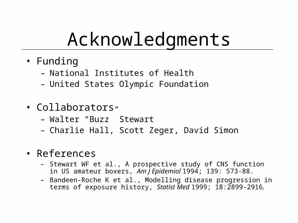
Scientific Question: Does boxing cause cerebral injury?
• Hypothesized pathway: brain jarring NEURO- PSYCHOLOGIC
OUTCOMES BOXING BRAIN CEREBRAL ELECTRO-BOUTS* JARRING INJURY PHYSIOLOGICSPAR OUTCOMES
NEUROLOGICOUTCOMES
---------------------------------------------------
SYMPTOMSEXPOSURE DOSE PHYSIOLOGIC
IMPAIRMENT SIGNS
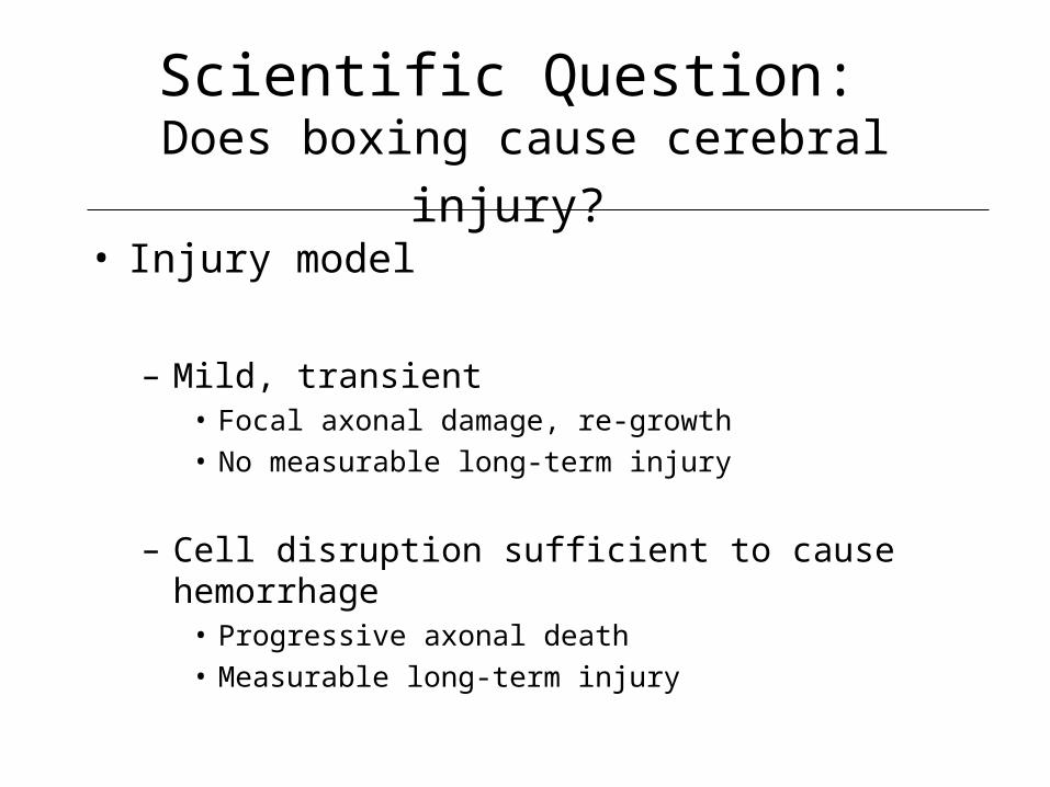
Scientific Question: Does boxing cause cerebral injury?
• Injury model
– Mild, transient• Focal axonal damage, re-growth• No measurable long-term injury
– Cell disruption sufficient to cause hemorrhage• Progressive axonal death• Measurable long-term injury

Brief Study Design• "Full" Boxing club sample
– NY, DC, Cleveland, St. Louis, Louisiana, Houston
• N = 593 boxers – One baseline and three follow-up exams “per boxer”; 1988-1994– N=493 with a first follow up
• Outcomes – 17 neuropsychological tests (Today: Block
Design)– Electrophysiologic Battery– Ataxia and Neurological Tests
• Covariates– Primary: number of bouts boxed– Secondary: age, race, education, Ravens IQ score, club,
non-boxing concussion history, drug test result
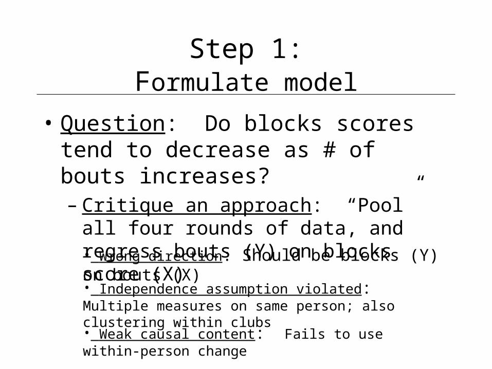
Step 1:Formulate model
• Question: Do blocks scores tend to decrease as # of bouts increases?– Critique an approach: “Pool” all four
rounds of data, and regress bouts (Y) on blocks score (X)
• Wrong direction: Should be blocks (Y) on bouts (X)
• Independence assumption violated: Multiple measures on same person; also clustering within clubs
• Weak causal content: Fails to use within-person change
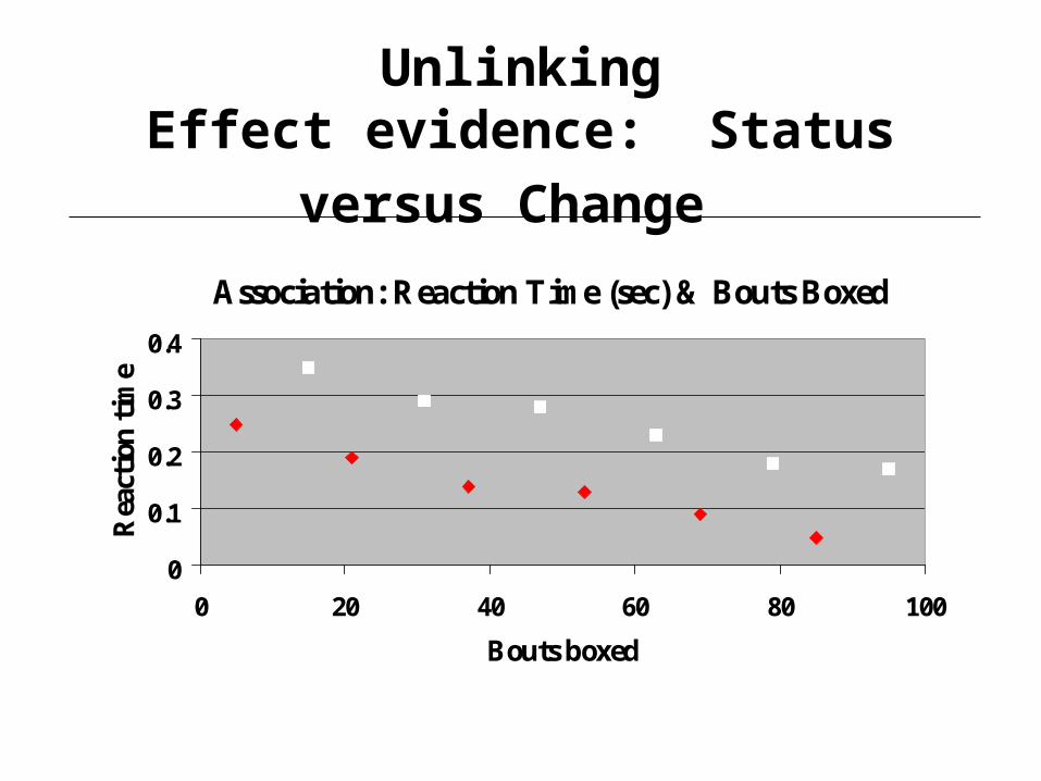
UnlinkingEffect evidence: Status
versus Change Association: Reaction Time (sec) & Bouts Boxed
0
0.1
0.2
0.3
0.4
0 20 40 60 80 100
Bouts boxed
Rea
ctio
n t
ime
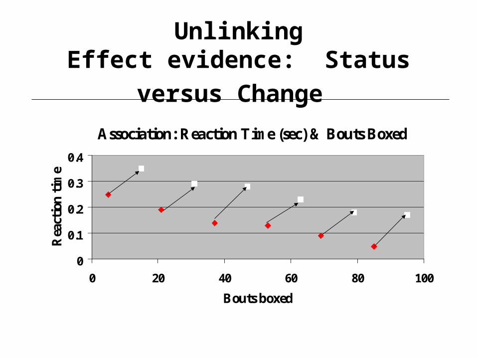
UnlinkingEffect evidence: Status
versus Change Association: Reaction Time (sec) & Bouts Boxed
0
0.1
0.2
0.3
0.4
0 20 40 60 80 100
Bouts boxed
Rea
ctio
n t
ime
Model Building
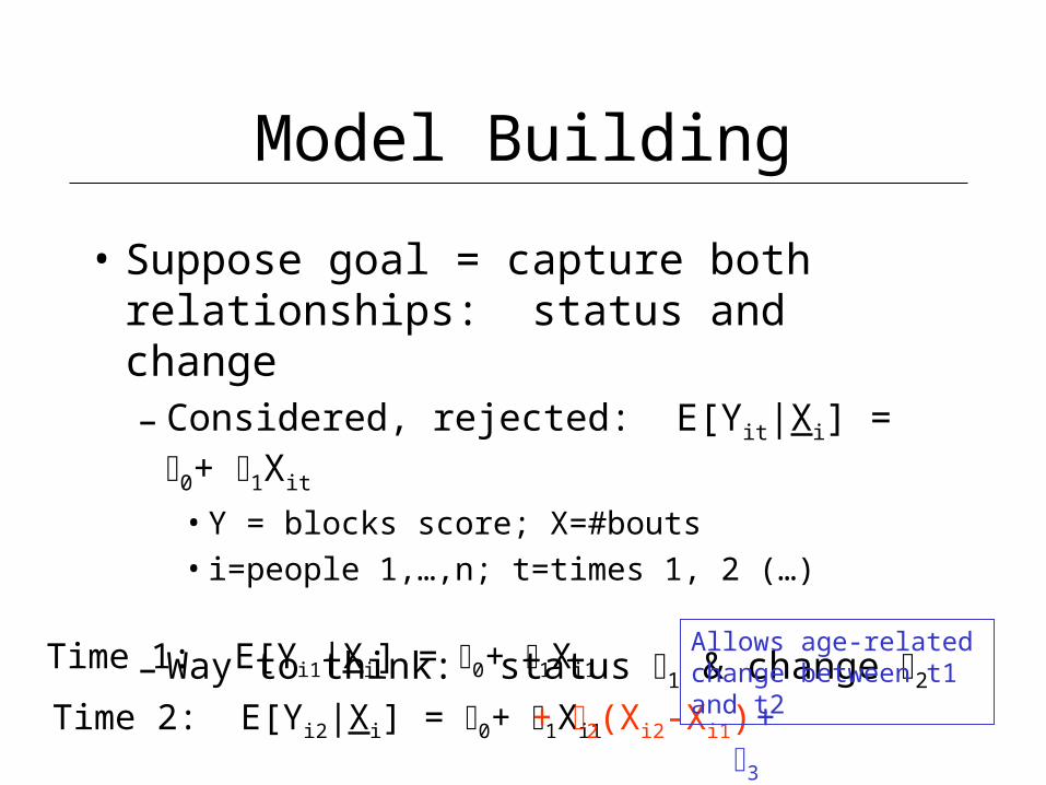
• Suppose goal = capture both relationships: status and change– Considered, rejected: E[Yit|Xi] = 0+ 1Xit
• Y = blocks score; X=#bouts• i=people 1,…,n; t=times 1, 2 (…)
– Way to think: status 1 & change 2 Time 1: E[Yi1|Xi] = 0+ 1Xi1
+ 3Time 2: E[Yi2|Xi] = 0+ 1Xi1 + 2(Xi2-Xi1)
Allows age-related change between t1 and t2
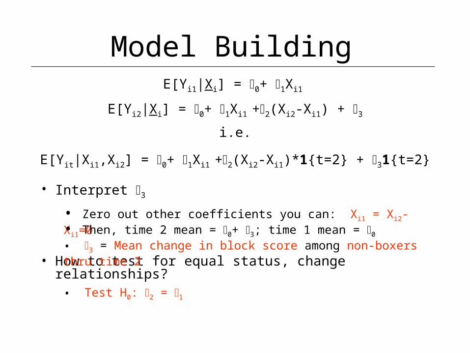
Model BuildingE[Yi1|Xi] = 0+ 1Xi1
E[Yi2|Xi] = 0+ 1Xi1 +2(Xi2-Xi1) + 3
i.e.
E[Yit|Xi1,Xi2] = 0+ 1Xi1 +2(Xi2-Xi1)*1{t=2} + 31{t=2}
• Interpret 3
• How to test for equal status, change relationships?f
• Zero out other coefficients you can: Xi1 = Xi2-Xi1=0• Then, time 2 mean = 0+ 3; time 1 mean = 0
• 3 = Mean change in block score among non-boxers thru time 2
• Test H0: 2 = 1
Model Building
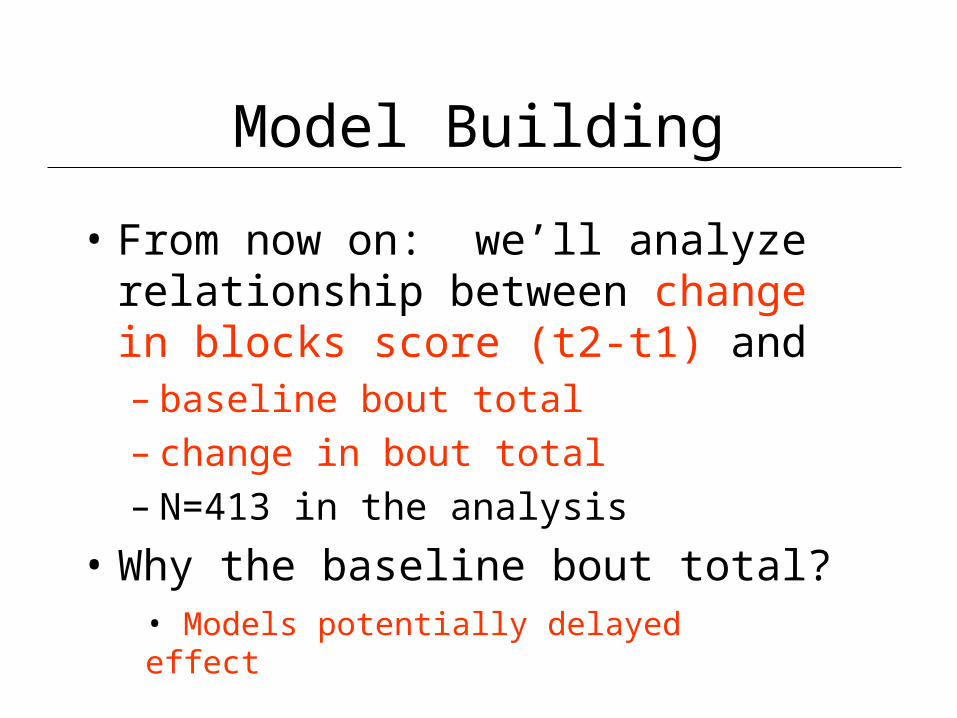
• From now on: we’ll analyze relationship between change in blocks score (t2-t1) and – baseline bout total– change in bout total– N=413 in the analysis
• Why the baseline bout total?• Models potentially delayed effect
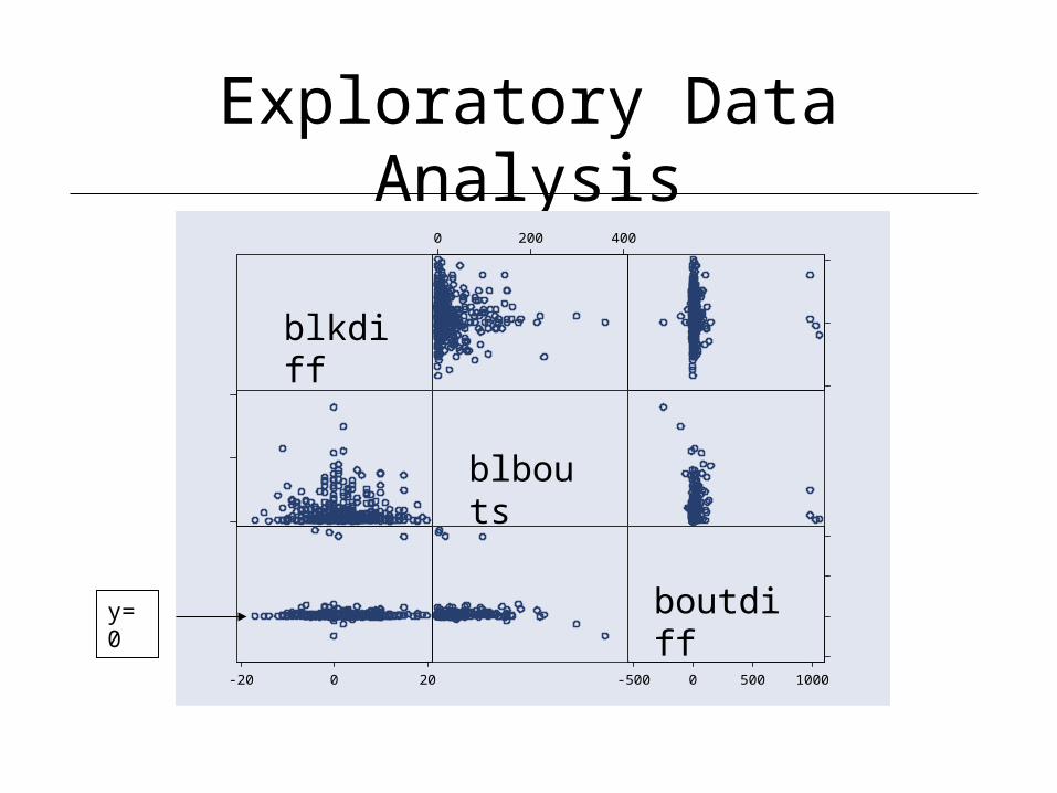
Exploratory Data Analysis
blkdiff
blbouts
boutdiff
-20
0
20
-20 0 20
0
200
400
0 200 400
-500
0
500
1000
-500 0 500 1000
blkdiff
blbouts
boutdiffy=0
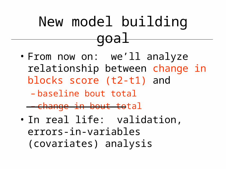
New model building goal
• From now on: we’ll analyze relationship between change in blocks score (t2-t1) and – baseline bout total– change in bout total
• In real life: validation, errors-in-variables (covariates) analysis
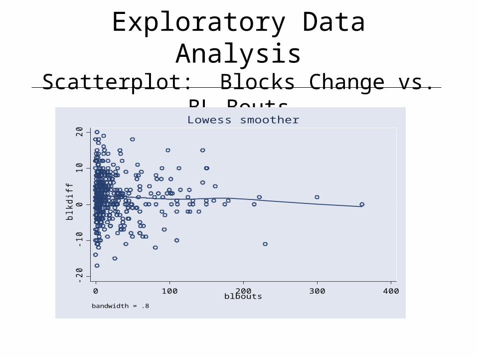
Exploratory Data AnalysisScatterplot: Blocks Change vs. BL Bouts
-20
-10
010
20
blk
diff
0 100 200 300 400blbouts
bandwidth = .8
Lowess smoother
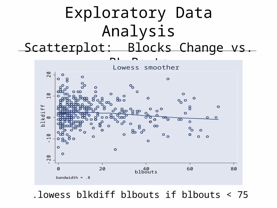
Exploratory Data AnalysisScatterplot: Blocks Change vs. BL Bouts
-20
-10
010
20
blk
diff
0 20 40 60 80blbouts
bandwidth = .8
Lowess smoother
.lowess blkdiff blbouts if blbouts < 75
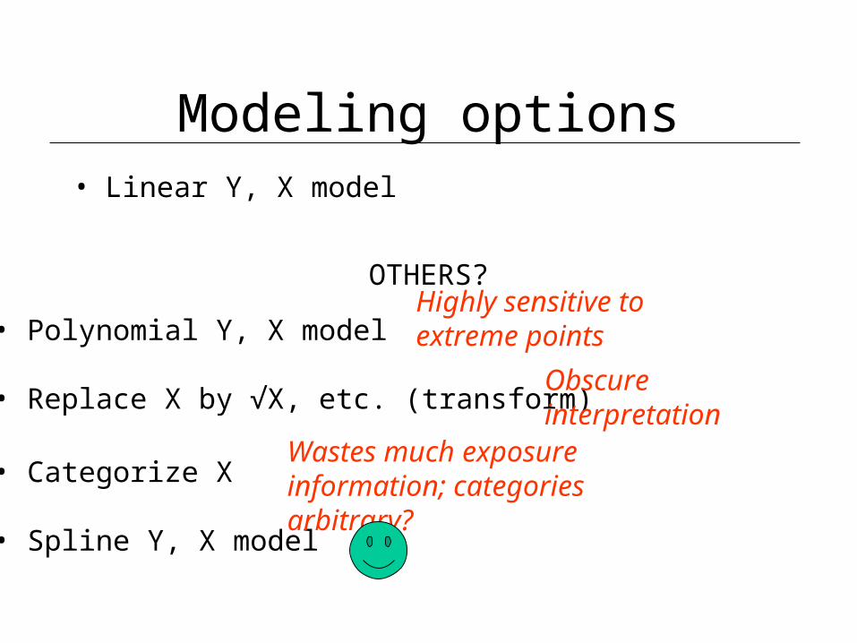
Modeling options• Linear Y, X model
OTHERS?
• Polynomial Y, X model
• Replace X by √X, etc. (transform)
• Categorize X
• Spline Y, X model
Highly sensitive to extreme points
Obscure interpretation
Wastes much exposure information; categories arbitrary?
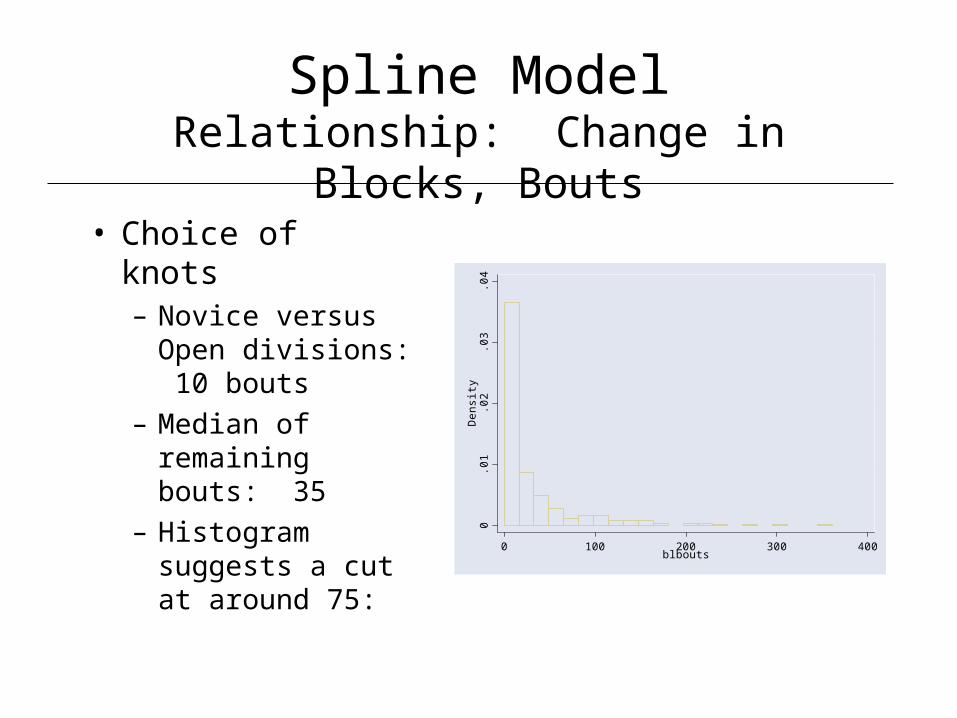
Spline ModelRelationship: Change in Blocks, Bouts
• Choice of knots– Novice versus
Open divisions: 10 bouts
– Median of remaining bouts: 35
– Histogram suggests a cut at around 75:
0.0
1.0
2.0
3.0
4D
ensi
ty
0 100 200 300 400blbouts
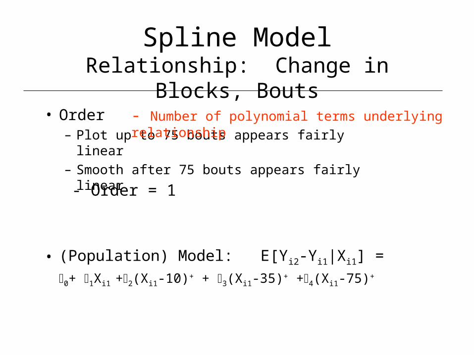
Spline ModelRelationship: Change in Blocks, Bouts
• Order– Plot up to 75 bouts appears fairly linear– Smooth after 75 bouts appears fairly linear
• (Population) Model: E[Yi2-Yi1|Xi1] =
0+ 1Xi1 +2(Xi1-10)+ + 3(Xi1-35)+ +4(Xi1-75)+
- Order = 1
- Number of polynomial terms underlying relationship
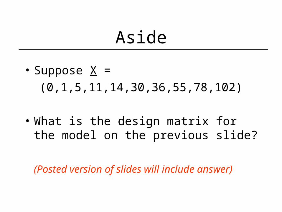
Aside
• Suppose X =
(0,1,5,11,14,30,36,55,78,102)
• What is the design matrix for the model on the previous slide?
(Posted version of slides will include answer)
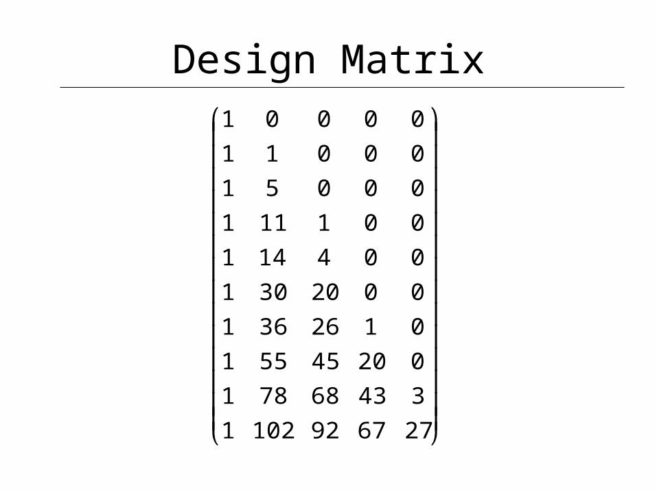
Design Matrix
2767921021
34368781
02045551
0126361
0020301
004141
001111
00051
00011
00001
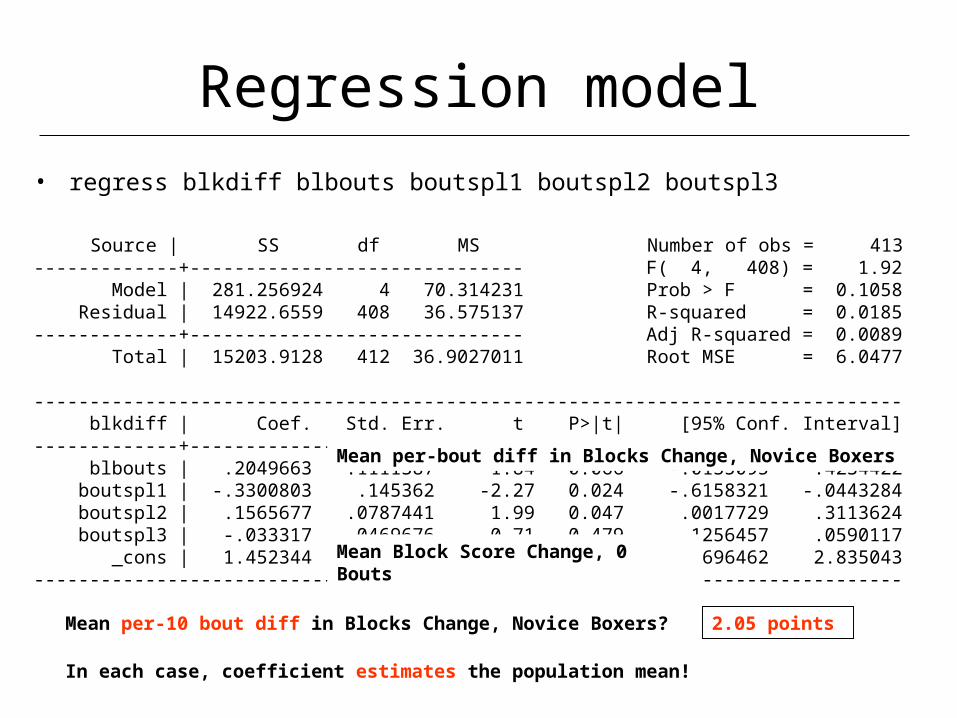
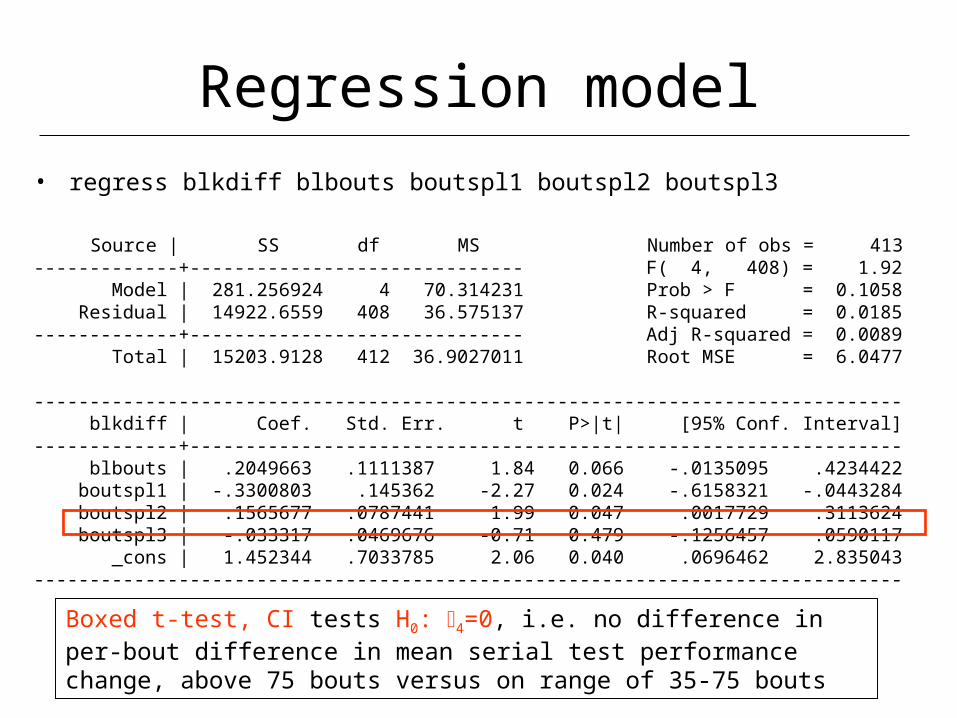
Regression model• regress blkdiff blbouts boutspl1 boutspl2 boutspl3
Source | SS df MS Number of obs = 413-------------+------------------------------ F( 4, 408) = 1.92 Model | 281.256924 4 70.314231 Prob > F = 0.1058 Residual | 14922.6559 408 36.575137 R-squared = 0.0185-------------+------------------------------ Adj R-squared = 0.0089 Total | 15203.9128 412 36.9027011 Root MSE = 6.0477
------------------------------------------------------------------------------ blkdiff | Coef. Std. Err. t P>|t| [95% Conf. Interval]-------------+---------------------------------------------------------------- blbouts | .2049663 .1111387 1.84 0.066 -.0135095 .4234422 boutspl1 | -.3300803 .145362 -2.27 0.024 -.6158321 -.0443284 boutspl2 | .1565677 .0787441 1.99 0.047 .0017729 .3113624 boutspl3 | -.033317 .0469676 -0.71 0.479 -.1256457 .0590117 _cons | 1.452344 .7033785 2.06 0.040 .0696462 2.835043------------------------------------------------------------------------------
Mean Block Score Change, 0 Bouts
Mean per-bout diff in Blocks Change, Novice Boxers
Mean per-10 bout diff in Blocks Change, Novice Boxers? 2.05 points
In each case, coefficient estimates the population mean!
Regression model• regress blkdiff blbouts boutspl1 boutspl2 boutspl3
Source | SS df MS Number of obs = 413-------------+------------------------------ F( 4, 408) = 1.92 Model | 281.256924 4 70.314231 Prob > F = 0.1058 Residual | 14922.6559 408 36.575137 R-squared = 0.0185-------------+------------------------------ Adj R-squared = 0.0089 Total | 15203.9128 412 36.9027011 Root MSE = 6.0477
------------------------------------------------------------------------------ blkdiff | Coef. Std. Err. t P>|t| [95% Conf. Interval]-------------+---------------------------------------------------------------- blbouts | .2049663 .1111387 1.84 0.066 -.0135095 .4234422 boutspl1 | -.3300803 .145362 -2.27 0.024 -.6158321 -.0443284 boutspl2 | .1565677 .0787441 1.99 0.047 .0017729 .3113624 boutspl3 | -.033317 .0469676 -0.71 0.479 -.1256457 .0590117 _cons | 1.452344 .7033785 2.06 0.040 .0696462 2.835043------------------------------------------------------------------------------
Boxed t-test, CI tests H0: 4=0, i.e. no difference in per-bout difference in mean serial test performance change, above 75 bouts versus on range of 35-75 bouts
Regression model
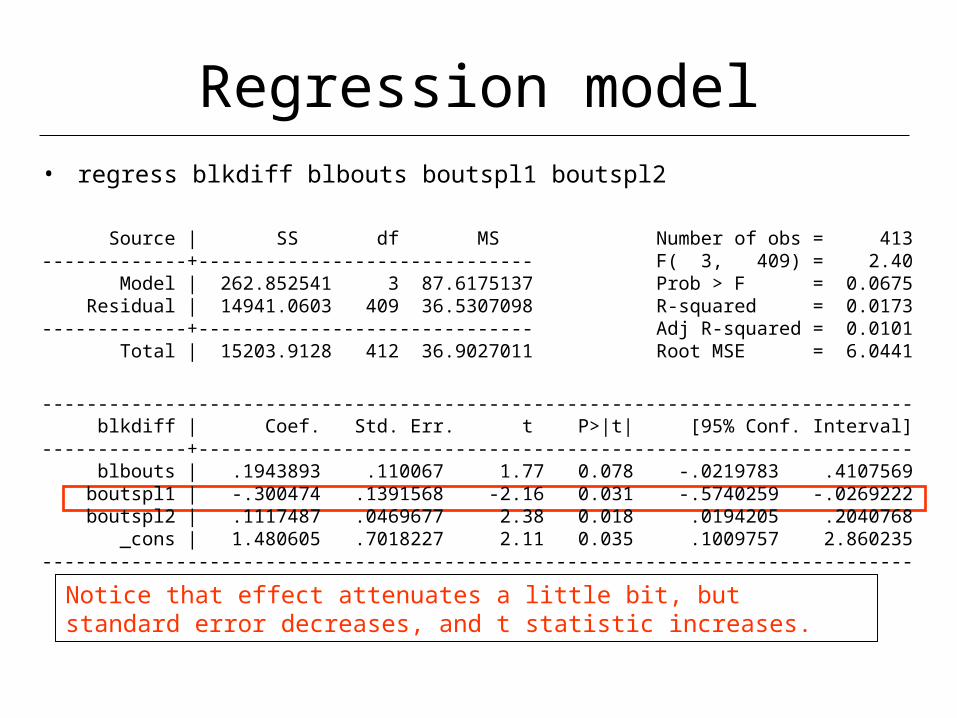
Notice that effect attenuates a little bit, but standard error decreases, and t statistic increases.
• regress blkdiff blbouts boutspl1 boutspl2
Source | SS df MS Number of obs = 413-------------+------------------------------ F( 3, 409) = 2.40 Model | 262.852541 3 87.6175137 Prob > F = 0.0675 Residual | 14941.0603 409 36.5307098 R-squared = 0.0173-------------+------------------------------ Adj R-squared = 0.0101 Total | 15203.9128 412 36.9027011 Root MSE = 6.0441
------------------------------------------------------------------------------ blkdiff | Coef. Std. Err. t P>|t| [95% Conf. Interval]-------------+---------------------------------------------------------------- blbouts | .1943893 .110067 1.77 0.078 -.0219783 .4107569 boutspl1 | -.300474 .1391568 -2.16 0.031 -.5740259 -.0269222 boutspl2 | .1117487 .0469677 2.38 0.018 .0194205 .2040768 _cons | 1.480605 .7018227 2.11 0.035 .1009757 2.860235------------------------------------------------------------------------------
What is good, bad about the estimates?
• The good– Accuracy (estimator is unbiased if correct
mean model; SEs are accurate if correct A1-A4)
– Precision (estimator is BLUE)
• The bad– Not terribly robust (may be influenced by
isolated points)
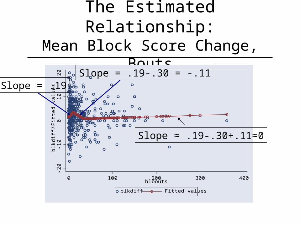
The Estimated Relationship:Mean Block Score Change, Bouts
-20
-10
010
20
blk
diff
/Fitt
ed v
alu
es
0 100 200 300 400blbouts
blkdiff Fitted values
Slope = .19Slope = .19-.30 = -.11
Slope ≈ .19-.30+.11≈0
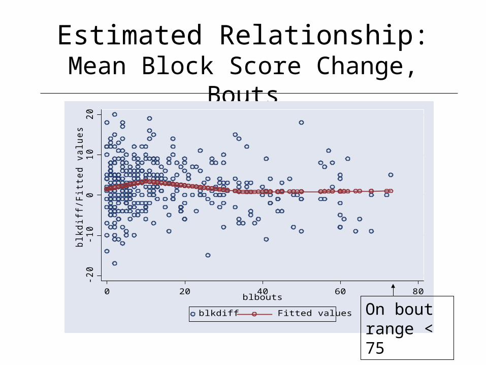
Estimated Relationship:Mean Block Score Change, Bouts
-20
-10
010
20
blk
diff/F
itte
d v
alu
es
0 20 40 60 80blbouts
blkdiff Fitted values On bout range < 75
Comments
• Odd finding: Apparent benefit of novice boxing, and loss of benefit (back to nominal) in early open boxing
• Checked for influence: Little• Are we being misled by relationships
with other variables?– Age– BL blocks design score
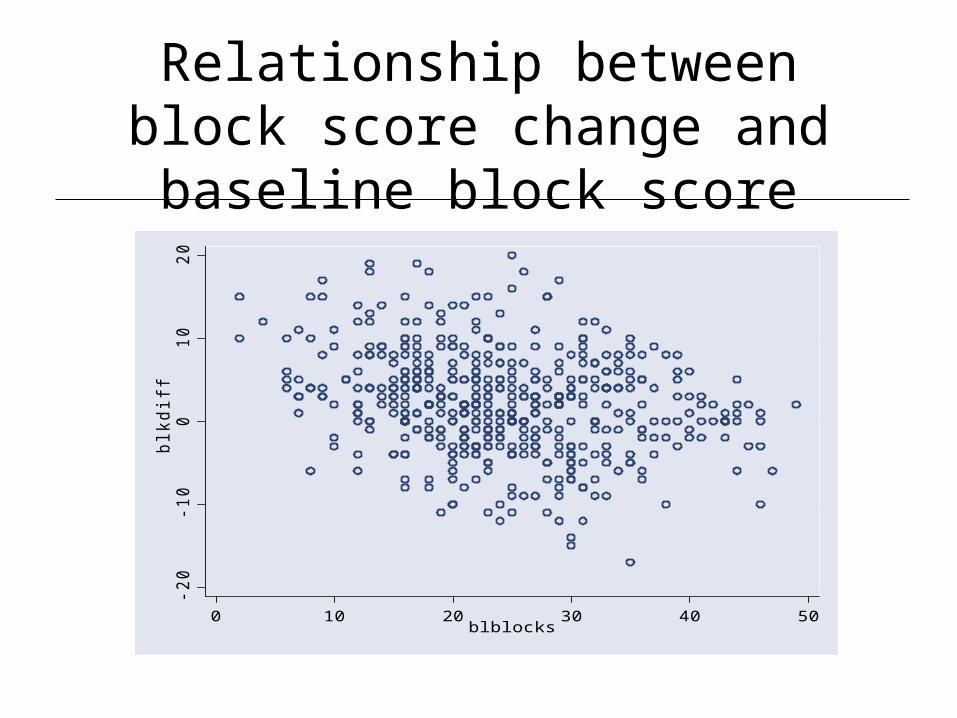
Relationship between block score change and baseline block score
-20
-10
010
20
blk
diff
0 10 20 30 40 50blblocks
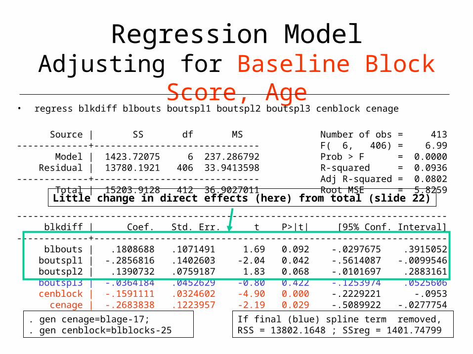
Regression ModelAdjusting for Baseline Block Score, Age
• regress blkdiff blbouts boutspl1 boutspl2 boutspl3 cenblock cenage
Source | SS df MS Number of obs = 413-------------+------------------------------ F( 6, 406) = 6.99 Model | 1423.72075 6 237.286792 Prob > F = 0.0000 Residual | 13780.1921 406 33.9413598 R-squared = 0.0936-------------+------------------------------ Adj R-squared = 0.0802 Total | 15203.9128 412 36.9027011 Root MSE = 5.8259
------------------------------------------------------------------------------ blkdiff | Coef. Std. Err. t P>|t| [95% Conf. Interval]-------------+---------------------------------------------------------------- blbouts | .1808688 .1071491 1.69 0.092 -.0297675 .3915052 boutspl1 | -.2856816 .1402603 -2.04 0.042 -.5614087 -.0099546 boutspl2 | .1390732 .0759187 1.83 0.068 -.0101697 .2883161 boutspl3 | -.0364184 .0452629 -0.80 0.422 -.1253974 .0525606 cenblock | -.1591111 .0324602 -4.90 0.000 -.2229221 -.0953 cenage | -.2683838 .1223957 -2.19 0.029 -.5089922 -.0277754
Little change in direct effects (here) from total (slide 22)
. gen cenage=blage-17;
. gen cenblock=blblocks-25If final (blue) spline term removed, RSS = 13802.1648 ; SSreg = 1401.74799
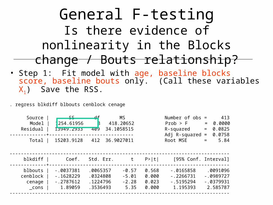
General F-testingIs there evidence of nonlinearity in the Blocks change / Bouts relationship?
• Step 1: Fit model with age, baseline blocks score, baseline bouts only. (Call these variables X1) Save the RSS.
. regress blkdiff blbouts cenblock cenage
Source | SS df MS Number of obs = 413 Model | 1254.61956 3 418.20652 Prob > F = 0.0000
Residual | 13949.2933 409 34.1058515 R-squared = 0.0825-------------+------------------------------ Adj R-squared = 0.0758 Total | 15203.9128 412 36.9027011 Root MSE = 5.84
------------------------------------------------------------------------------ blkdiff | Coef. Std. Err. t P>|t| [95% Conf. Interval]-------------+---------------------------------------------------------------- blbouts | -.0037381 .0065357 -0.57 0.568 -.0165858 .0091096 cenblock | -.1628229 .0324808 -5.01 0.000 -.2266731 -.0989727 cenage | -.2787612 .1224796 -2.28 0.023 -.5195294 -.0379931 _cons | 1.89059 .3536493 5.35 0.000 1.195393 2.585787------------------------------------------------------------------------------
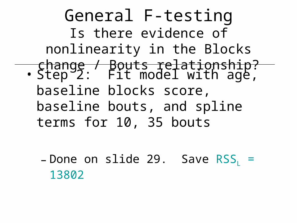
General F-testingIs there evidence of nonlinearity in the Blocks change / Bouts relationship?
• Step 2: Fit model with age, baseline blocks score, baseline bouts, and spline terms for 10, 35 bouts
– Done on slide 29. Save RSSL = 13802
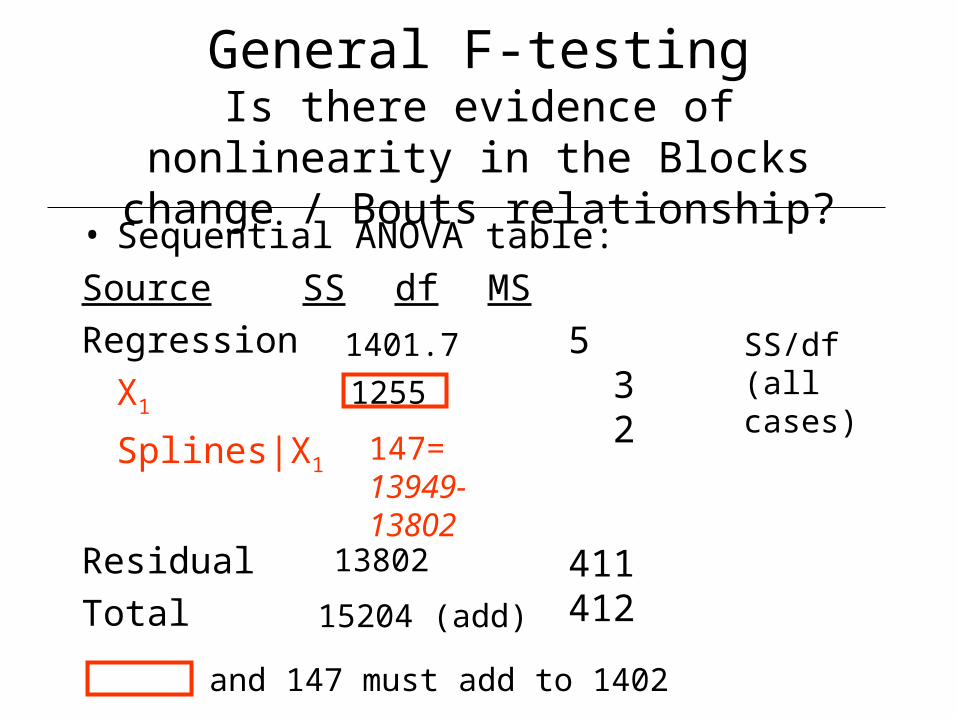
General F-testingIs there evidence of nonlinearity in the Blocks change / Bouts relationship?
• Sequential ANOVA table:
Source SS df MS
Regression
X1
Splines|X1
Residual
Total
13802
1401.7
15204 (add)
147= 13949-13802
1255
and 147 must add to 1402
5 3 2
411412
SS/df(all cases)
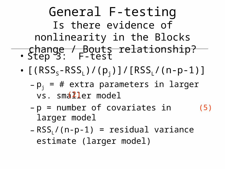
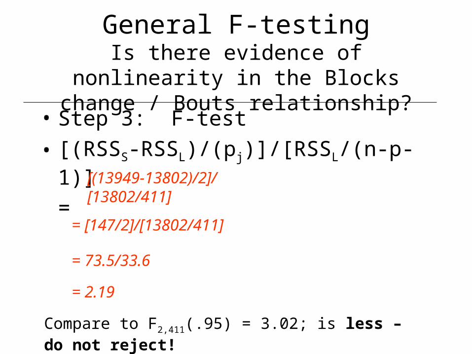
General F-testingIs there evidence of nonlinearity in the Blocks change / Bouts relationship?
• Step 3: F-test
• [(RSSS-RSSL)/(pj)]/[RSSL/(n-p-1)]
– pj = # extra parameters in larger vs. smaller model
– p = number of covariates in larger model
– RSSL/(n-p-1) = residual variance estimate (larger model)
(2)
(5)
General F-testingIs there evidence of nonlinearity in the Blocks change / Bouts relationship?
• Step 3: F-test
• [(RSSS-RSSL)/(pj)]/[RSSL/(n-p-1)]
= [(13949-13802)/2]/[13802/411]
= [147/2]/[13802/411]
= 73.5/33.6
= 2.19
Compare to F2,411(.95) = 3.02; is less – do not reject!
Summary
• Little evidence of relationship between boxing exposure and subsequent longitudinal decline or improvement in visuo-spatial ability as measured by the Blocks score
• More work to elucidate longitudinal relationship between exposure accrual and changes in ability is needed