Embed Size (px)
Citation preview

Biostat 200 Lecture 3
1

Announcements• Reminder – Assignment 1 due this Thursday• Send via e-mail to your TA
Last name A-L TAs: Jeff Edwards and Vicky KeoleianRoom 6702 Send assignments as Word docs to: [email protected] Last name M-Z TAs: Christine Fox and Karen OrdovasRoom 6704 Send assignments as Word docs to: [email protected]
2

Today’s topics
•Review of some probability facts•Check in on what you should have learned so far•Probability distributions
3
From last lecture: Independence vs. mutual exclusivity
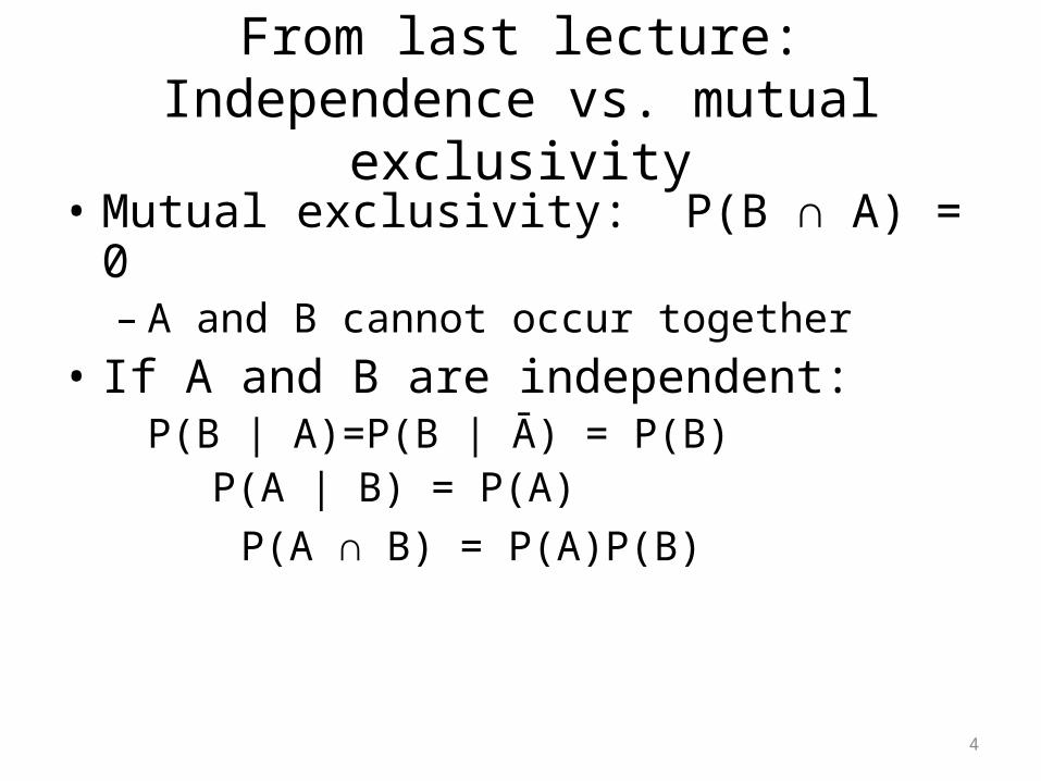
• Mutual exclusivity: P(B ∩ A) = 0– A and B cannot occur together
• If A and B are independent: P(B | A)=P(B | Ā) = P(B)
P(A | B) = P(A) P(A ∩ B) = P(A)P(B)
4

From last lecture: Independence vs. mutual exclusivity
– If A and B are independent: – A and B can still co-occur but A has no bearing on
B – A and B are not mutually exclusive
5

6

What you should have learned from the past 2 weeks
• Types of variables• The ability to perform in Stata and understand:
– Basic manipulation of data, opening and saving data sets and .do files, basic data cleaning
– Basic summaries relevant to different types of variables
– Basic graphical analyses of different types of variables• Basic probability concepts, especially conditional
probability, mutual exclusivity, and independence
7
Where we go from here• Use probability concepts to discuss theoretical
distributions• Knowing (or assuming) that a variable follows a certain
distribution, you can calculate the probability of observing a certain value for that variable
• Next week: Use the Central Limit Theorem to examine the probability distribution of sample means (the normal distribution)
• Knowing the distribution of a sample mean allows us to calculate the probability of observing a particular sample mean
• We will extend these concepts to examine differences in means and proportions between two or more groups (hypothesis testing) 8

Why do we care about probability distributions?
• Probability distributions describe the possible values of a random variable
• Many statistical tests are based on probability distributions
9
Probability distributions
• Variables whose outcome can occur by chance, i.e. are not fixed, are called random variables
• Probability distributions describe the possible values of the random variable
10

• For discrete variables the probability distribution describes the probability of each possible value
• For example, consider the experiment in which you flip a coin 2 times and count the number of heads. – The possible outcomes of the experiment are: HH,
TH, HT, TT. – You want to focus on the number of heads, which
could be 0,1, or 2. The probability of each outcome is:
Number of heads Probability
0 .25
1 .5
2 .25
11

• The table looks similar to a frequency table of the data, but it is actually the theoretical distribution
• If you perform an infinite number of experiments, your data will look like this table
Number of heads Relative frequency
0 .25
1 .5
2 .25
12
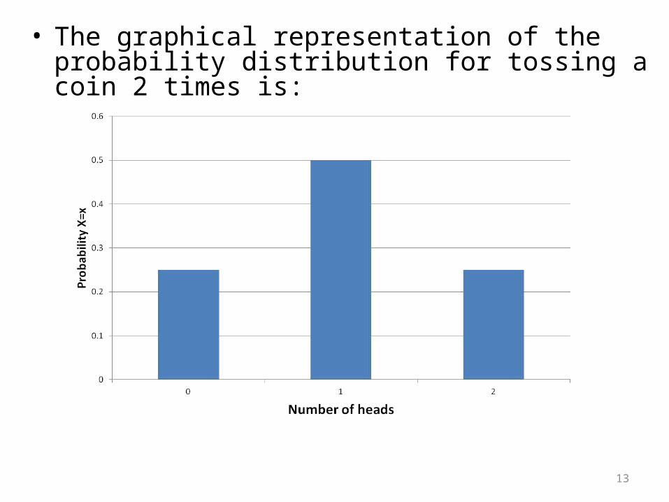
• The graphical representation of the probability distribution for tossing a coin 2 times is:
13

• Note that the probabilities add to 1. This is true of all probability distributions.
• This is a theoretical probability distribution based on our understanding of coin tossing– The probability of a head on each toss is .5– The probability of heads on the first toss is
independent of the second toss– It’s actually the binomial distribution
• We can write down a formula for P(X=x)
14

• We can use this theoretical distribution to make predictions about future experiments
• E.g. The probability that there will be at least 1 head in a trial of 2 coin tosses P(X≥1) = P(X=1) + P(X=2)
(by what probability rule?) = .5 +.25 = .75
15

• If you performed the experiment once, you’d get 0,1, or 2 heads
• Performing the experiment 10 times: 2, 1, 1, 1, 1, 0, 0, 0, 1, 1
• What if we did the experiment 100 times?1000 times? What would the frequency
distribution for the outcomes look like?
Number of heads Frequency (%)
0 3 (30)
1 6 (60)
2 1 (10)
16
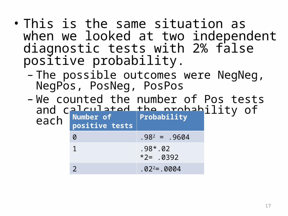
• This is the same situation as when we looked at two independent diagnostic tests with 2% false positive probability.– The possible outcomes were NegNeg, NegPos,
PosNeg, PosPos– We counted the number of Pos tests and calculated
the probability of each
Number of positive tests
Probability
0 .982 = .9604
1 .98*.02 *2= .0392
2 .022=.0004
17

• The graphical representation of the probability distribution for number of false positive tests is:
18
Empirical Probability distributions• Empirical probability distributions are based on
real data
• They are usually based on a large sample or complete enumeration of a population
• The probabilities are calculated from the relative frequencies of the data
19

Probability distributions
• For discrete variables the probability distribution describes the probability of each possible value
• For continuous variables, the distribution describes the probability of a range of values
20
Bernoulli random variable• If you have a variable that can take on one of two values with
a constant probability p, then it is a Bernoulli random variable
• If the proportion of people in the population with a disease (the prevalence) is 15%, then when you randomly select one person, the probability that he/she has the disease is
P(Y=1)=p= 0.15 And the probability that a randomly selected person does
not have the disease isP(Y=0)=1-p =0.85
21
Bernoulli distribution
• A Bernoulli random variable follows the Bernoulli distribution
• p is the parameter that characterizes the distribution• The Bernoulli distribution is a discrete distribution –
the outcomes are either 0 or 1• It describes only one trial – so really is more
theoretical than practical – it is the building block to describe the distribution of more than one trial
22

Binomial distribution
• Example: The proportion of people in the population with the disease (the prevalence) is 15%, then P(Y=1)=0.15 and P(Y=0)=0.85.
• If we take a random sample of 5 people from this population, there will be 0,1,2,3,4, or 5 people with the disease.
• If the probability of disease in each person is independent, then we can write down the probability of each of these outcomes even before we draw the sample. 23

For example, the probability that ALL of them will have the disease is P(X=5):
=P(X1=1)* P(X2=1)* P(X3=1)* P(X4=1)* P(X5=1)
= 0.15 x 0.15 x 0.15 x 0.15 x 0.15 = 0.00008 by the multiplication rule for independent
outcomes P(A ∩ B)=P(A)P(B)
24

For example, the probability that NONE of them will have the disease is P(X=0):
=P(X1=0)* P(X2=0)* P(X3=0)* P(X4=0)* P(X5=0)
=0.85 x 0.85 x 0.85 x 0.85 x 0.85 = 0.444
25
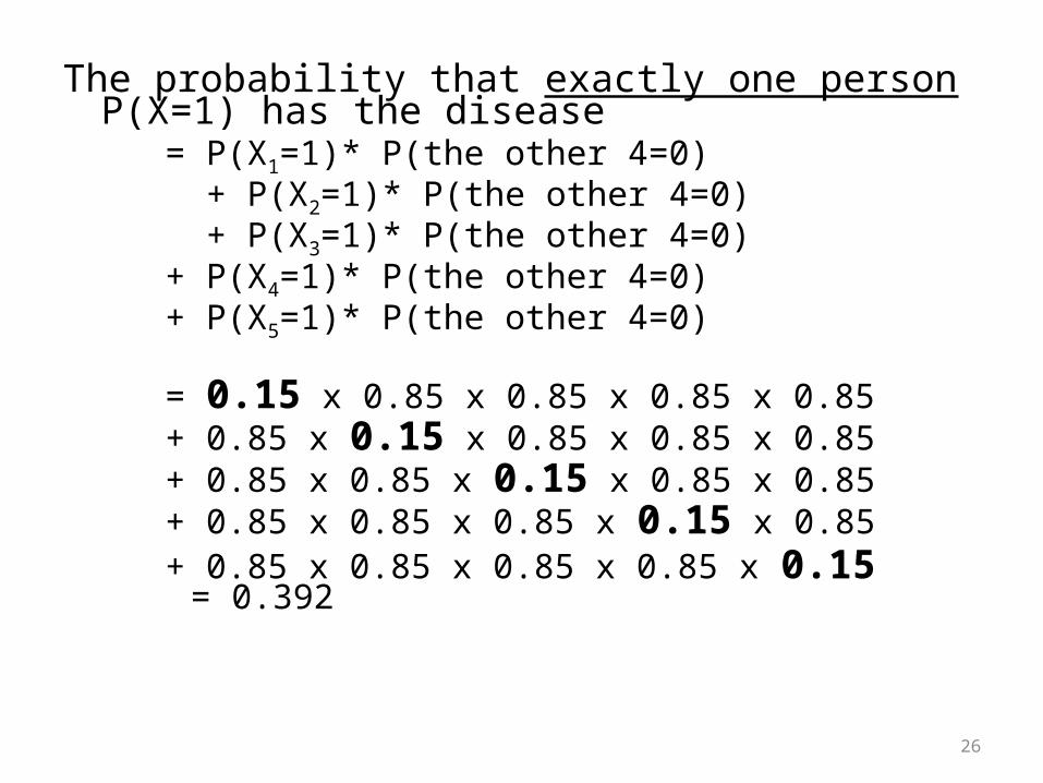
The probability that exactly one person P(X=1) has the disease
= P(X1=1)* P(the other 4=0) + P(X2=1)* P(the other 4=0) + P(X3=1)* P(the other 4=0) + P(X4=1)* P(the other 4=0) + P(X5=1)* P(the other 4=0)
= 0.15 x 0.85 x 0.85 x 0.85 x 0.85 + 0.85 x 0.15 x 0.85 x 0.85 x 0.85 + 0.85 x 0.85 x 0.15 x 0.85 x 0.85 + 0.85 x 0.85 x 0.85 x 0.15 x 0.85 + 0.85 x 0.85 x 0.85 x 0.85 x 0.15 = 0.392
26
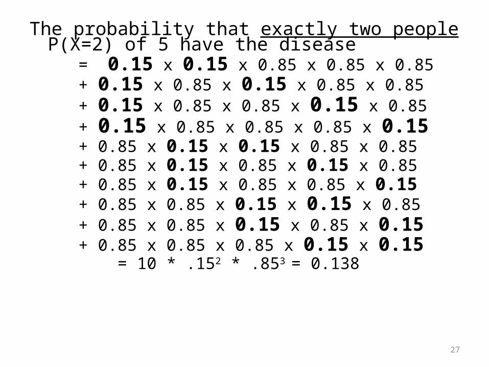
The probability that exactly two people P(X=2) of 5 have the disease
= 0.15 x 0.15 x 0.85 x 0.85 x 0.85 + 0.15 x 0.85 x 0.15 x 0.85 x 0.85+ 0.15 x 0.85 x 0.85 x 0.15 x 0.85+ 0.15 x 0.85 x 0.85 x 0.85 x 0.15 + 0.85 x 0.15 x 0.15 x 0.85 x 0.85+ 0.85 x 0.15 x 0.85 x 0.15 x 0.85+ 0.85 x 0.15 x 0.85 x 0.85 x 0.15+ 0.85 x 0.85 x 0.15 x 0.15 x 0.85+ 0.85 x 0.85 x 0.15 x 0.85 x 0.15+ 0.85 x 0.85 x 0.85 x 0.15 x 0.15 = 10 * .152 * .853 = 0.138
27
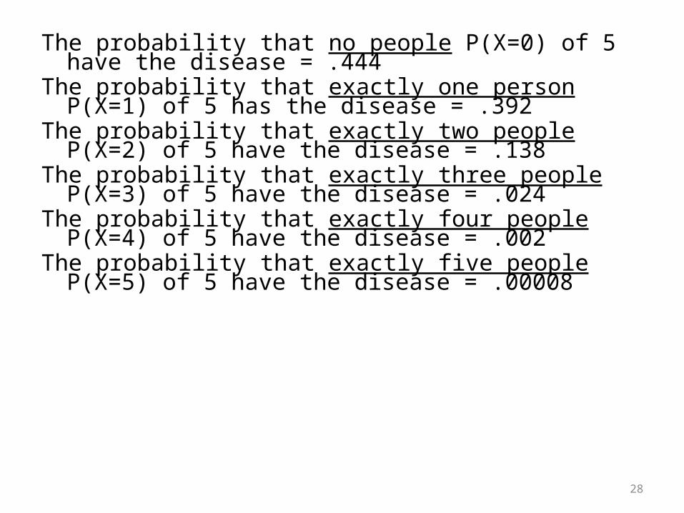
The probability that no people P(X=0) of 5 have the disease = .444
The probability that exactly one person P(X=1) of 5 has the disease = .392
The probability that exactly two people P(X=2) of 5 have the disease = .138
The probability that exactly three people P(X=3) of 5 have the disease = .024
The probability that exactly four people P(X=4) of 5 have the disease = .002
The probability that exactly five people P(X=5) of 5 have the disease = .00008
28

What do these probabilities sum to? 29

The probability that exactly one person P(X=1) has the disease
P(X=1, n=5, p=0.15) = 0.15 x 0.85 x 0.85 x 0.85 x 0.85 + 0.85 x 0.15 x 0.85 x 0.85 x 0.85 + 0.85 x 0.85 x 0.15 x 0.85 x 0.85 + 0.85 x 0.85 x 0.85 x 0.15 x 0.85 + 0.85 x 0.85 x 0.85 x 0.85 x 0.15 = 0.392
= 5 * .151 *.854
= 5 * p1 * (1-p)4
5 is the number of different ways you could get one success in the 5 “trials”
30
Binomial distribution
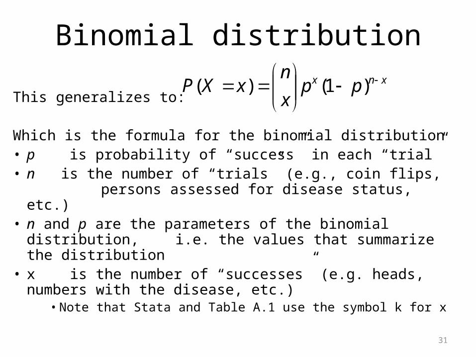
This generalizes to:
Which is the formula for the binomial distribution• p is probability of “success” in each “trial”• n is the number of “trials” (e.g., coin flips,
persons assessed for disease status, etc.)• n and p are the parameters of the binomial distribution,
i.e. the values that summarize the distribution• x is the number of “successes” (e.g. heads,
numbers with the disease, etc.)• Note that Stata and Table A.1 use the symbol k for x
xnx ppx
nxXP
)1()(
31

Binomial distribution• Assumptions:
– There are a fixed number of trials n, each of which results in one of two mutually exclusive outcomes
– The outcomes of the n trials are independent
– The probability of success p is constant for each trial
32
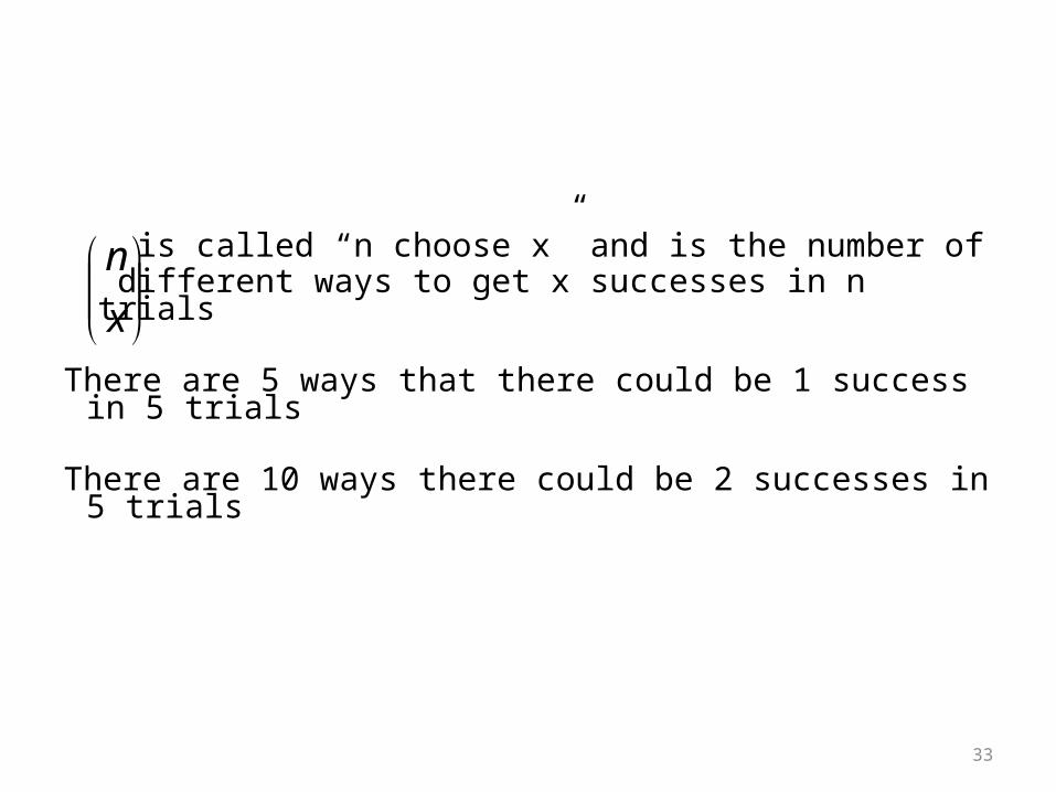
is called “n choose x” and is the number of different ways to get x successes in n trials
There are 5 ways that there could be 1 success in 5 trials
There are 10 ways there could be 2 successes in 5 trials
x
n
33
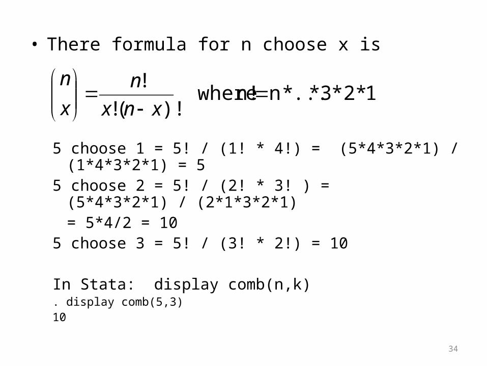
• There formula for n choose x is
5 choose 1 = 5! / (1! * 4!) = (5*4*3*2*1) / (1*4*3*2*1) = 5 5 choose 2 = 5! / (2! * 3! ) = (5*4*3*2*1) / (2*1*3*2*1)
= 5*4/2 = 10 5 choose 3 = 5! / (3! * 2!) = 10
In Stata: display comb(n,k). display comb(5,3)10
1*2*3*...*n n! where)!(!
!
xnx
n
x
n
34
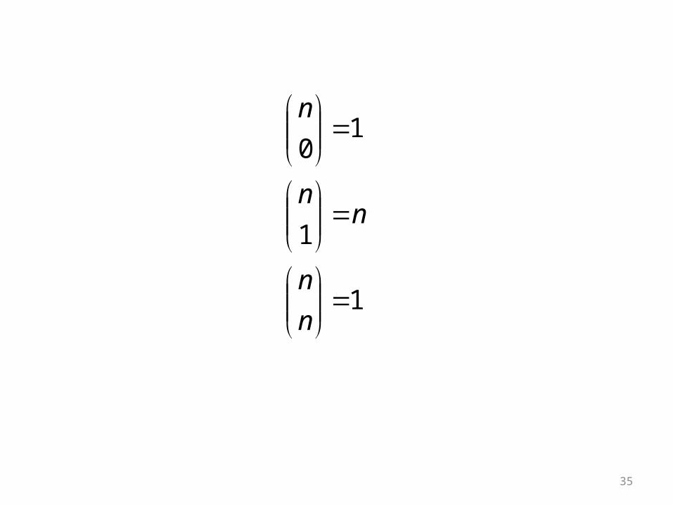
1
1
10
n
n
nn
n
35
• Ways to find binomial probabilities– The previous equations– Table A.1 in the textbook– Stata
• Binomialp(n,k,p)• Binomialtail(n,k,p)
36
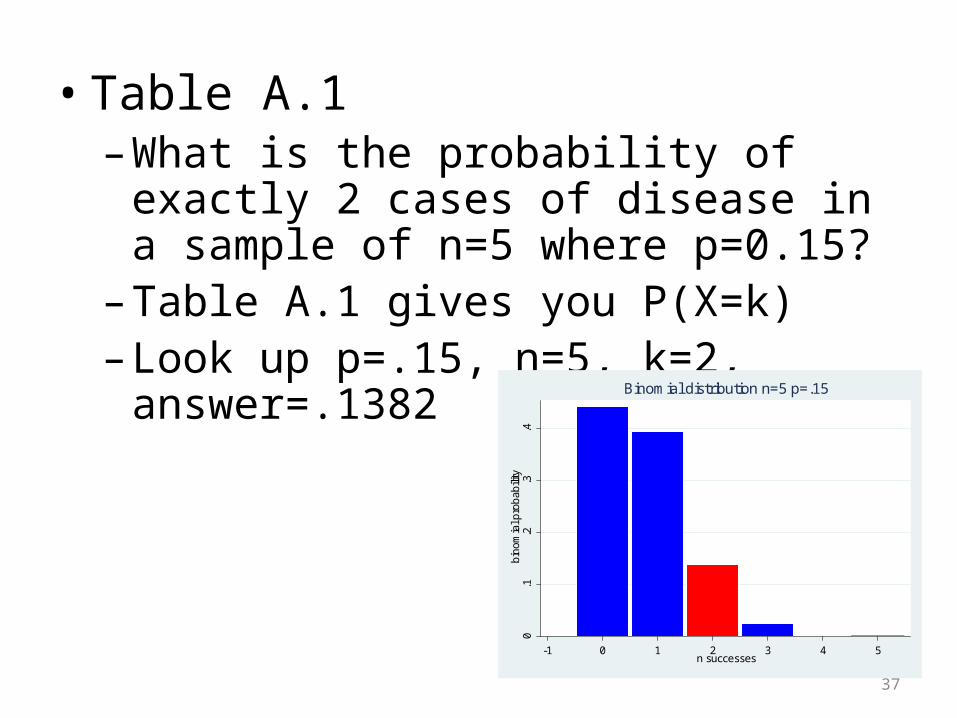
• Table A.1– What is the probability of exactly 2 cases of
disease in a sample of n=5 where p=0.15?– Table A.1 gives you P(X=k)– Look up p=.15, n=5, k=2, answer=.1382
37
0.1
.2.3
.4b
inom
ial p
rob
abili
ty
-1 0 1 2 3 4 5n successes
Binomial distribution n=5 p=.15
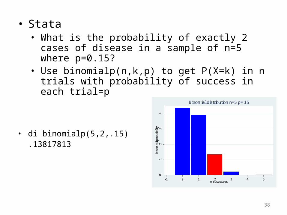
• Stata• What is the probability of exactly 2 cases of disease in a
sample of n=5 where p=0.15?• Use binomialp(n,k,p) to get P(X=k) in n trials with
probability of success in each trial=p
• di binomialp(5,2,.15).13817813
38
0.1
.2.3
.4b
inom
ial p
rob
abili
ty
-1 0 1 2 3 4 5n successes
Binomial distribution n=5 p=.15

• What is the probability of 1 or more cases of disease in a sample of n=5 where p=0.15?
• Remember Table A.1 gives you P(X=k). • We want P(X≥k)• One way would be to look up all the
probabilities: P(X=1)+P(X=2)+ ... +P(X=5)• But remember P(X≥1) = 1-P(X=0) • Looking up P(X=0) we get 0.4437
– So 1-P(X=0) = 1- 0.4437 = 0.5563
39
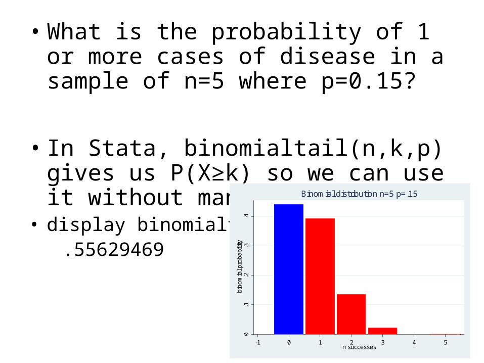
• What is the probability of 1 or more cases of disease in a sample of n=5 where p=0.15?
• In Stata, binomialtail(n,k,p) gives us P(X≥k) so we can use it without manipulation
• display binomialtail(5,1,.15) .55629469
40
0.1
.2.3
.4b
inom
ial p
rob
abili
ty
-1 0 1 2 3 4 5n successes
Binomial distribution n=5 p=.15
• The binomial distribution can be used to calculate the probability of observing at least X successes, or cases of disease, etc, in a population of size n in which the true probability of disease is p.
• Example. The Cambodia prevalence of TB infection is 495 per 100,000 (0.00495), yet there have been 7 cases in a school of 1000 children (0.007). You wonder how this compares to the national prevalence.
• Prob would see 7 or more cases in 1000 students if p=.00495?
41

• Prob would see 7 or more cases in a school of 1000 if p=.00495?display binomialtail(1000,7,.00495)
.23016477
What if there had been 20 cases?
Prob would see 20 or more cases in a school of 1000 if p=0.00495?
binomialtail(1000,20,.00495)
2.654e-07
What might you conclude?
42
Binomial distribution
• The mean of a binomially distributed random variable X is np
• This means that over an large number of samples of size n with probability p of success, the mean number of successes (X) over the samples will be approximately np
43

Binomial distribution• The variance of a binomially distributed random
variable X is n*p*(1-p)• This means that over a large number of samples
of size n, the sample variance of the X’s will be approximately n*p*(1-p)
44

• So for our example with n=5 and p=.15, the mean is:
• The variance is:• The standard deviation is:
45

Binomial distribution• Binomial mean = np• Binomial variance= np(1-p)
– Variance is largest when p=0.5, smaller when p closer to 0 or 1
– The distribution is symmetric when p=0.5– The distribution is a mirror image for 1-p (i.e. the
distribution for p=0.05 is the mirror image of the one for p=0.95)
46

0.1
.2.3
.4bi
nom
ial p
roba
bilit
y
0 2 4 6 8 10 12 14 16 18 20n successes
Binomial distribution n=20 p=.05
0.1
.2.3
.4bi
nom
ial p
roba
bilit
y
0 2 4 6 8 10 12 14 16 18 20n successes
Binomial distribution n=20 p=.950
.05
.1.1
5.2
bino
mia
l pro
babi
lity
0 2 4 6 8 10 12 14 16 18 20n successes
Binomial distribution n=20 p=.5
P(X=2) ?P(X≥2) ?
47

Poisson distribution• A discrete distribution to model rare events
occurring in time or space • Unlike the binomial distribution, it is not based on a
series of trials, and there is no theoretical limit to the number of events that can occur
• However, when n is large and p is small, it does act like the binomial
• The Poisson has only one parameter, λ, that is the mean number of events (and also the variance)
48

Normal distribution
• Used for continuous variables that cover the entire range, i.e. values can take on 1.432, -72.12
• Classic bell shaped curve• Values can span from -∞ to ∞• Unimodal and symmetric, so the mean is also
equal to the median and mode
49
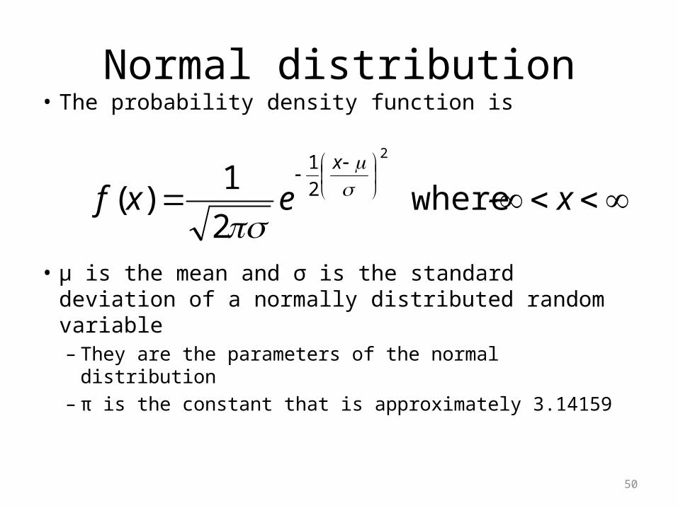
Normal distribution• The probability density function is
• μ is the mean and σ is the standard deviation of a normally distributed random variable– They are the parameters of the normal distribution– π is the constant that is approximately 3.14159
x -exf
x
where2
1)(
2
2
1
50
• Note that the left hand side of the equation is f(x) and not P(X=x)
• Why?– For a discrete distribution, the sum of the bars
equals 1– For a continuous distribution, the area under the
curve equals one– A continuous variable X can take on an infinite
number of values, therefore P(X=x)=0
51
• If X has a normal distribution with mean μ and standard deviation σ we write
X ~ N(μ, σ) • Many variables are approximately normally
distributed• We can use the distribution to calculate
probabilities associated with such variables
52
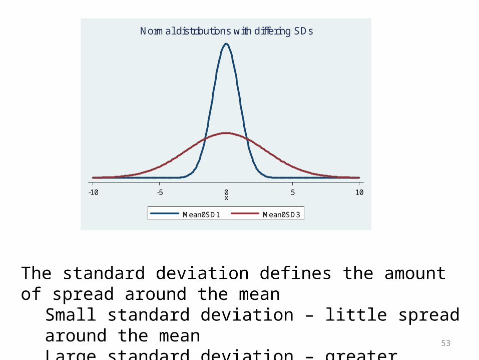
The standard deviation defines the amount of spread around the mean
Small standard deviation – little spread around the meanLarge standard deviation – greater spread around the mean
-10 -5 0 5 10x
Mean0SD1 Mean0SD3
Normal distributions with differing SDs
53

-10 -8 -6 -4 -2 0 2 4 6 8 10x
Mean0SD1 Mean0SD3Mean4SD1
Several normal distributions
54
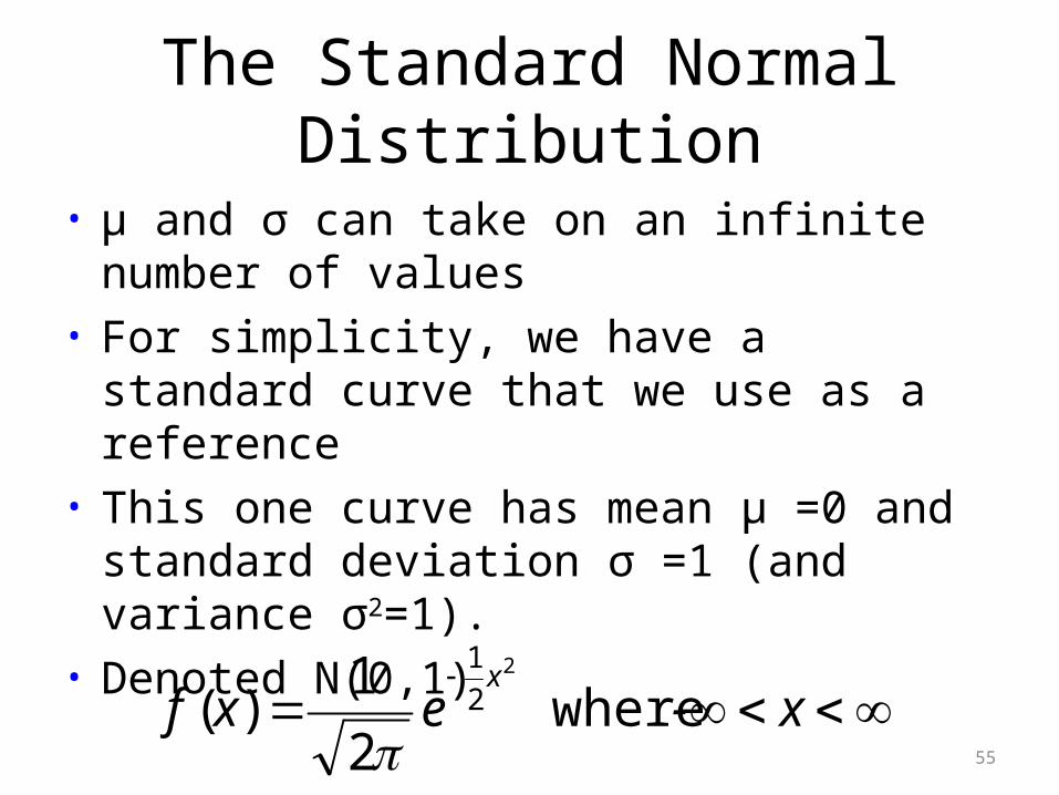
The Standard Normal Distribution
• μ and σ can take on an infinite number of values
• For simplicity, we have a standard curve that we use as a reference
• This one curve has mean μ =0 and standard deviation σ =1 (and variance σ2=1).
• Denoted N(0,1)
55
x -exfx
where2
1)(
2
2
1

The Standard Normal Distribution
• If X is a normally distributed random variable with mean μ and standard deviation σ then
Z= (X – μ)/σ
is a standard normal random variable
• That is, a normally distributed random variable with its mean subtracted off, divided by its standard deviation, is a normal random variable with mean=0 and standard deviation=1
56

The Standard Normal Distribution• If X ~ N(μ, σ) then
• Z= (X- μ) / σ ~ N(0, 1)
57
0.1
.2.3
.4y
-5 -4 -3 -2 -1 0 1 2 3 4 5Z
Standard normal curve
•We can use theoretical distributions to determine the probability of particular values of random variables
• For the binomial distribution, we added probabilities of the assumed distribution to calculate the probability of observing a certain number (k) of events (or more).
•Remember the probability of observing 1 or more disease cases in a sample of 5 was
P(X=1) + P(X=2) + P(X=3) + P(X=4) + P(X=5)
58

•However, for a continuous variable, because there are an infinite number of values of x, we can’t calculate P(X=x).
•However, we can calculate P(X ≥ x), which is the area under the normal curve from x to infinity
•The area under curves is calculated by taking the integral
2
1)()(
2
2
1
x x
x
dxexfxXP
59

For Z ~ N(0,1) P(Z≥0) = 0.50
60
-5 -4 -3 -2 -1 0 1 2 3 4 5Z
Standard normal distribution
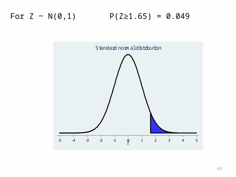
For Z ~ N(0,1) P(Z≥1.65) = 0.049
61
-5 -4 -3 -2 -1 0 1 2 3 4 5Z
Standard normal distribution

For Z ~ N(0,1) P(Z≥1.96) = 0.025
62
-5 -4 -3 -2 -1 0 1 2 3 4 5Z
Standard normal distribution

For Z ~ N(0,1) P(Z<-1.96) = 0.025
Z is symmetric
63
-5 -4 -3 -2 -1 0 1 2 3 4 5Z
Standard normal distribution
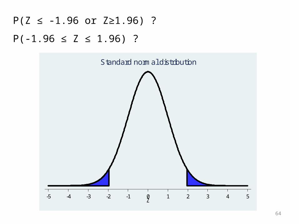
P(Z ≤ -1.96 or Z≥1.96) ?
P(-1.96 ≤ Z ≤ 1.96) ?
64
-5 -4 -3 -2 -1 0 1 2 3 4 5Z
Standard normal distribution
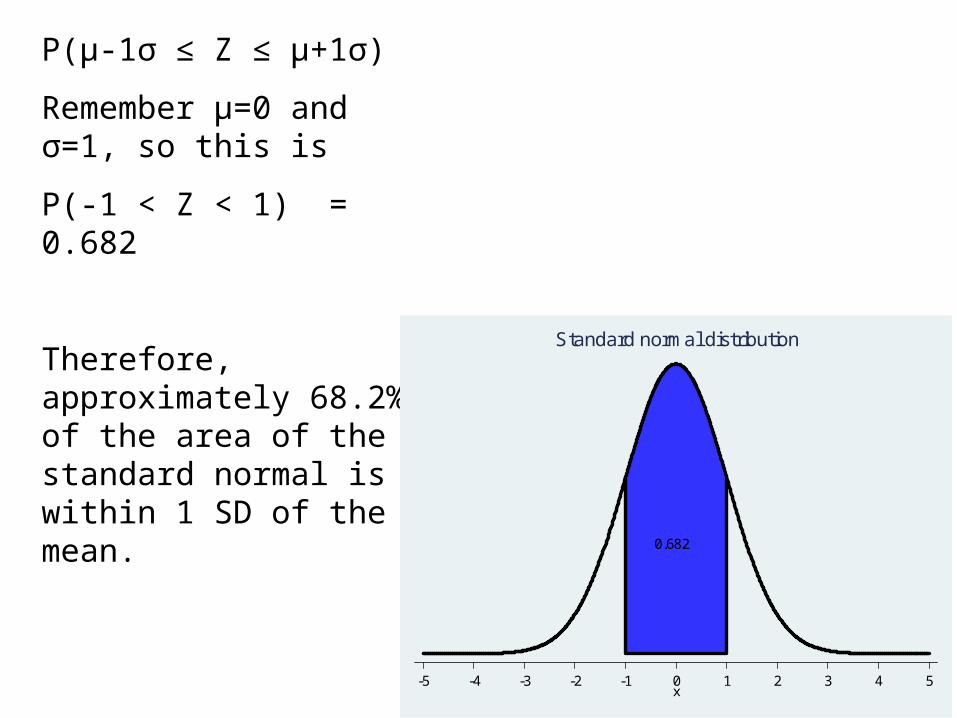
P(µ-1σ ≤ Z ≤ µ+1σ)
Remember µ=0 and σ=1, so this is
P(-1 < Z < 1) = 0.682
Therefore, approximately 68.2% of the area of the standard normal is within 1 SD of the mean.
0.1590.159
65
0.682
-5 -4 -3 -2 -1 0 1 2 3 4 5x
Standard normal distribution

P(µ-2σ ≤ Z ≤ µ+2σ)
Remember µ=0 and σ=1, so this is
P(-2 < Z < 2) = 0.954
Therefore, approximately 95.4% of the area of the standard normal is within 2 SD of the mean.
0.0230.023
66
0.954
-5 -4 -3 -2 -1 0 1 2 3 4 5Z
Standard normal distribution

•Stata will calculate standard normal probabilities for you
•In Stata, the left portion of the curve P(Z<z) is calculated for you.display normal(1.96).9750021
•If you want the right hand portion of the curve, P(Z>z), you subtract your answer from 1display 1-normal(1.96).0249979
•If you want the middle: display normal(1.96) -normal(-1.96).95000421
67
-5 -4 -3 -2 -1 0 1 2 3 4 5Z
Prob Z<1.96 highlighted
Standard normal distribution
• Standard normal tables, like A.3 in the book calculate the right hand portion of the curve for you, P(Z≥z)
• If you want P(Z≥1.96), look up z=1.9 in the rows and z=0.06 in the columns, and read off the probability : 0.025
• If you wanted P(Z<1.96), then you’d need to realize that this is the complement of P(Z ≥1.96), so the answer is 1-0.025=0.975.
• What if you want to find P(Z ≥4.23)?
68
Example• X is the distribution of systolic blood pressure in 18-74
y.o. US males ~N(129, 19.8)• What is the upper 2.5% value for blood pressure in this
population?• What is the value of z for which P(Z≥z)=0.025?• z=1.96• Transform back to the original units• z=1.96=(x-129)/19.8 • x=1.96*19.8 +129 =167.8 mm Hg
69
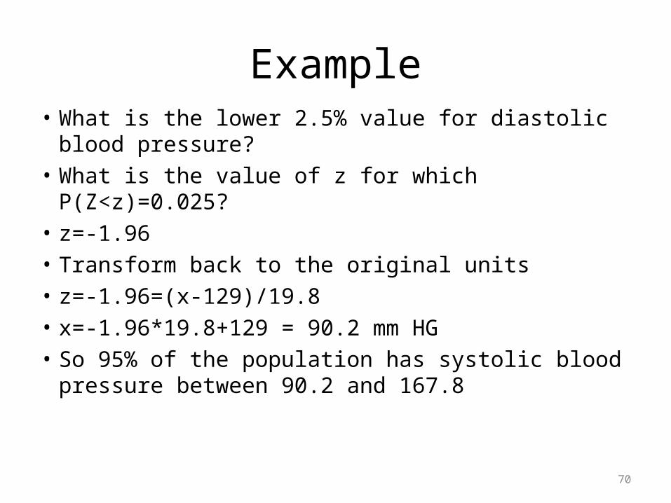
Example• What is the lower 2.5% value for diastolic blood
pressure?• What is the value of z for which P(Z<z)=0.025?• z=-1.96• Transform back to the original units• z=-1.96=(x-129)/19.8 • x=-1.96*19.8+129 = 90.2 mm HG• So 95% of the population has systolic blood pressure
between 90.2 and 167.8
70
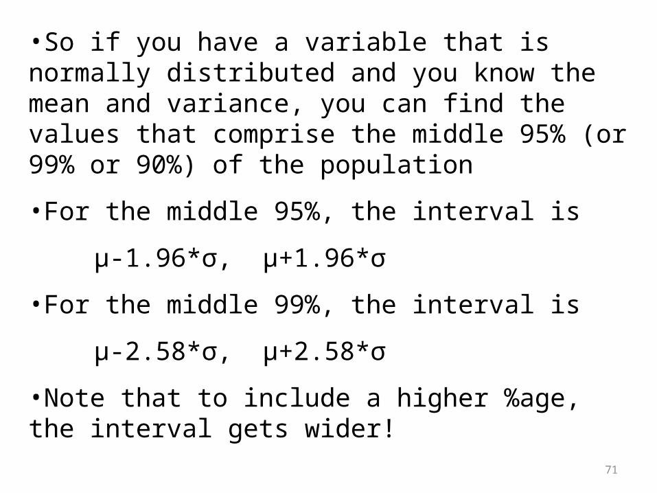
•So if you have a variable that is normally distributed and you know the mean and variance, you can find the values that comprise the middle 95% (or 99% or 90%) of the population
•For the middle 95%, the interval is
µ-1.96*σ, µ+1.96*σ
•For the middle 99%, the interval is
µ-2.58*σ, µ+2.58*σ
•Note that to include a higher %age, the interval gets wider!
71

Another example
• What is you wanted to know the proportion in the population with systolic blood pressure of over 150 mm Hg?
• Need to convert to a standard normal variable to get the probability
• z=(150-129)/19.8 = 1.06 This is the z-score or z-statistic
• P(Z>1.06)= .145
72
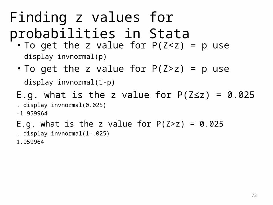
• To get the z value for P(Z<z) = p usedisplay invnormal(p)
• To get the z value for P(Z>z) = p usedisplay invnormal(1-p)
E.g. what is the z value for P(Z≤z) = 0.025. display invnormal(0.025)
-1.959964
E.g. what is the z value for P(Z>z) = 0.025. display invnormal(1-.025)
1.959964
Finding z values for probabilities in Stata
73
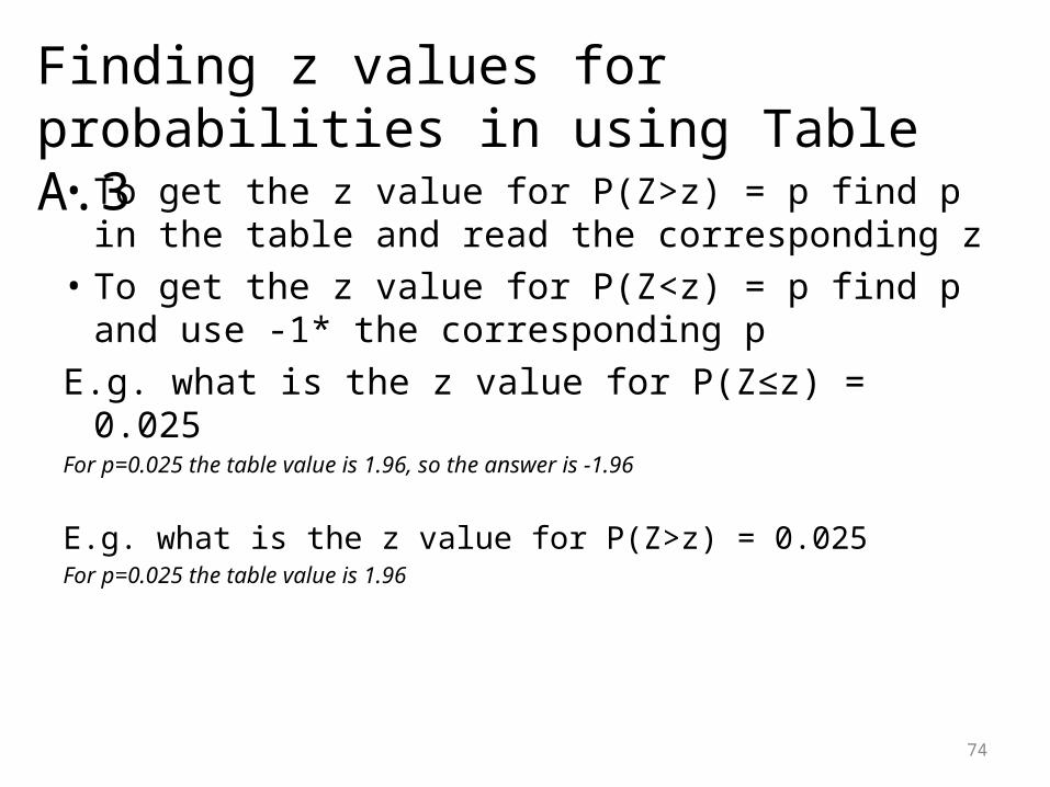
• To get the z value for P(Z>z) = p find p in the table and read the corresponding z
• To get the z value for P(Z<z) = p find p and use -1* the corresponding p
E.g. what is the z value for P(Z≤z) = 0.025For p=0.025 the table value is 1.96, so the answer is -1.96
E.g. what is the z value for P(Z>z) = 0.025For p=0.025 the table value is 1.96
Finding z values for probabilities in using Table A.3
74
Key points
• For discrete probability distributions, you can calculate P(X=x)
• The binomial distribution gives the probability of the number of successes in n trials P(X=x)
• For continuous probability distributions, you can only calculate P(X>x) or P(X<x)
• The normal distribution describes some continuous data – we’ll see some very useful properties next week
• We transform to the standard normal distribution in order to work with the probabilities
75

For next time
• We will review the binomial and normal distributions in lab and practice using them
• Read Pagano and Gauvreau– Chapter 7 (Review of today’s material)– Chapter 8, 9, and 14 (pages 324-329)
76